Learning Hash Functions Using Column Generation
Abstract
††* indicates equal contributions.Fast nearest neighbor searching is becoming an increasingly important tool in solving many large-scale problems. Recently a number of approaches to learning data-dependent hash functions have been developed. In this work, we propose a column generation based method for learning data-dependent hash functions on the basis of proximity comparison information. Given a set of triplets that encode the pairwise proximity comparison information, our method learns hash functions that preserve the relative comparison relationships in the data as well as possible within the large-margin learning framework. The learning procedure is implemented using column generation and hence is named CGHash. At each iteration of the column generation procedure, the best hash function is selected. Unlike most other hashing methods, our method generalizes to new data points naturally; and has a training objective which is convex, thus ensuring that the global optimum can be identified. Experiments demonstrate that the proposed method learns compact binary codes and that its retrieval performance compares favorably with state-of-the-art methods when tested on a few benchmark datasets.
1 Introduction
The explosive growth in the volume of data to be processed in applications such as web search and multimedia retrieval increasingly demands fast similarity search and efficient data indexing/storage techniques. Considerable effort has been spent on designing hashing methods which address both the issues of fast similarity search and efficient data storage (for example, (Andoni & Indyk, 2006; Weiss et al., 2008; Zhang et al., 2010b; Norouzi & Fleet, 2011; Kulis & Darrell, 2009; Gong et al., 2012)). A hashing-based approach constructs a set of hash functions that map high-dimensional data samples to low-dimensional binary codes. These binary codes can be easily loaded into the memory in order to allow rapid retrieval of data samples. Moreover, the pairwise Hamming distance between these binary codes can be efficiently computed by using bit operations, which are well supported by modern processors, thus enabling efficient similarity calculation on large-scale datasets. Hash-based approaches have thus found a wide range of applications, including object recognition (Torralba et al., 2008), information retrieval (Zhang et al., 2010b), local descriptor compression (Strecha et al., 2011), image matching (Korman & Avidan, 2011), and many more. Recently a number of effective hashing methods have been developed which construct a variety of hash functions, mainly on the assumption that semantically similar data samples should have similar binary codes, such as random projection-based locality sensitive hashing (LSH) (Andoni & Indyk, 2006), boosting learning-based similarity sensitive coding (SSC) (Shakhnarovich et al., 2003), and spectral hashing of Weiss et al. (2008) which is inspired by Laplacian eigenmap.
In more detail, spectral hashing (Weiss et al., 2008) optimizes a graph Laplacian based objective function such that in the learned low-dimensional binary space, the local neighborhood structure of the original dataset is best preserved. SSC (Shakhnarovich et al., 2003) makes use of boosting to adaptively learn an embedding of the original space, represented by a set of weak learners or hash functions. This embedding aims to preserve the pairwise affinity relationships of training duplets (i.e., pairs of samples in the original space). These approaches have demonstrated that, in general, data-dependent hashing is superior to data-independent hashing with a typical example being LSH (Andoni & Indyk, 2006).
Following this vein, here we learn hash functions using side information that is generally presented in a set of triplet-based constraints. Note that the triples used for training can be generated in an either supervised or unsupervised fashion. The fundamental idea is to learn optimal hash functions such that, when using the learned weighted Hamming distance, the relative distance comparisons of the form “point is closer to than to ” are satisfied as well as possible ( and are respectively relevant and irrelevant samples to ). This type of relative proximity comparisons have been successfully applied to learn quadratic distance metrics (Schultz & Joachims, 2004; Shen et al., 2012). Usually this type of proximity relationships do not require explicit class labels and thus are easier to obtain than either the class labels or the actual distances between data points. For instance, in content based image retrieval, to collect feedback, users may be required to report whether image looks more similar to than it is to a third image . This task is typically much easier than to label each individual image. Formally, we are given a set , where is some similarity measure (e.g., Euclidean distance in the original space; or semantic similarity measure provided by a user). As explained, one may not explicitly know ; instead, one may only be able to provide sparse proximity relationships. Using such a set of constraints, we formulate a learning problem in the large-margin framework. By using a convex surrogate loss function, a convex optimization problem is obtained, but has an exponentially large number of variables. Column generation is thus employed to efficiently and optimally solve the formulated optimization problem.
The main contribution of this work is to propose a novel hash function learning framework which has the following desirable properties. (i) The formulated optimization problem can be globally optimized. We show that column generation can be used to iteratively find the optimal hash functions. The weights of all the selected hash functions for calculating the weighted Hamming distance are updated at each iteration. (ii) The proposed framework is flexible and can accommodate various types of constraints. We show how to learn hash functions based on proximity comparisons. Furthermore, the framework can accommodate different types of loss functions as well as regularization terms. Also, our hashing framework can use different types of hash functions such as linear functions, decision stumps/trees, RBF kernel functions, etc.
Related work Loosely speaking, hashing methods may be categorized into two groups: data-independent and data-dependent. Without using any training data, data-independent hashing methods usually generate a set of hash functions using randomization. For instance, LSH of Andoni & Indyk (2006) use random projection and thresholding to generate binary codes in the Hamming space, where the mutually close data samples in the Euclidean space are likely to have similar binary codes. Recently, Kulis & Grauman (2009) propose a kernelized version of LSH, which is capable of capturing the intrinsic relationships between data samples using kernels instead of linear inner products. In terms of learning methodology, data-dependent hashing methods can make use of unsupervised, supervised or semi-supervised learning techniques to learn a set of hash functions that generate the compact binary codes. As for unsupervised learning, two typical approaches are used to obtain such compact binary codes, including thresholding the real-valued low-dimensional vectors (after dimensionality reduction) and direct optimization of a Hamming distance based objective function (e.g., spectral hashing (Weiss et al., 2008), self-taught hashing (Zhang et al., 2010b)). The spectral hashing (SPH) method directly optimizes a graph Laplacian objective function in the Hamming space. Inspired by SPH, Zhang et al. (2010b) developed the self-taught hashing (STH) method. At the first step of STH, Laplacian graph embedding is used to generate a sequence of binary codes for each sample. By viewing these binary codes as binary classification labels, a set of hash functions are obtained by training a set of bit-specific linear support vector machines. Liu et al. (2011) proposed a scalable graph-based hashing method which uses a small-size anchor graph to approximate the original neighborhood graph and alleviates the computational limitation of spectral hashing.
As for the supervised learning case, a number of hashing methods take advantage of labeled training samples to build data-dependent hash functions. These hashing methods often formulate hash function learning as a classification problem. For example, Salakhutdinov & Hinton (2009) proposed the restricted Boltzmann machine (RBM) hashing method using a multi-layer deep learning technique for binary code generation. Strecha et al. (2011) use Fisher linear discriminant analysis (LDA) to embed the original data samples into a lower-dimensional space, where the embedded data samples are binarized using thresholding. Boosting methods have also been employed to develop hashing methods such as SSC (Shakhnarovich et al., 2003) and Forgiving Hash (Baluja & Covell, 2008), both of which learn a set of weak learners as hash functions in the boosting framework. It is demonstrated in (Torralba et al., 2008) that some data-dependent hashing methods like stacked RBM and boosting SSC perform much better than LSH on large-scale databases of millions of images. Wang et al. (2012) proposed a semi-supervised hashing method, which aims to ensure the smoothness of similar data samples and the separability of dissimilar data samples. More recently, Liu et al. (2012) introduced a kernel-based supervised hashing method, where the hashing functions are nonlinear kernel functions.
The closest work to ours might be boosting based SSC hashing (Shakhnarovich et al., 2003), which also learns a set of weighted hash functions through boosting learning. Ours differs SSC in the learning procedure. The resulting optimization problem of our CGHash is based on the concept of margin maximization. We have derived a meaningful Lagrange dual problem such that column generation can be applied to solve the semi-infinite optimization problem. In contrast, SSC is built on the learning procedure of AdaBoost, which employs stage-wise coordinate-descent optimization. The weights associated with selected hash functions (corresponding weak classifiers in AdaBoost) are not fully updated at each iteration. Also the information used for training is different. We have used distance comparison information and SSC uses pairwise information. In addition, our work can accommodate various types of constraints, and can flexibly adapt to different types of loss functions as well as regularization terms. It is unclear, for example, how SSC can accommodate different types regularization that may encode useful prior information. In this sense our CGHash is much more flexible. Next, we present our main results.
2 The proposed algorithm
Given a set of training samples , (), we aim to learn a set of hash functions , for mapping these training samples to a low-dimensional binary space, being described by a set of binary codewords Here each is an -dimensional binary vectors. In the low-dimensional binary space, the codewords ’s are supposed to preserve the underlying proximity information of corresponding ’s in the original high-dimensional space. Next we learn such hash functions within the large-margin learning framework.
Formally, suppose that we are given a set of triplets with and being the triplet index set. These triplets encode the proximity comparison information such that the distance/dissimilarity between and is smaller than that between and . Now we need to define the weighted Hamming distance for the learned binary codes: where is a non-negative weight factor associated with the -th hash function. In our experiments, we have generated the triplets set as: and belong to the same class and and belong to different classes. As discussed, these triplets may be sparsely provided by users in applications such as image retrieval. So we want the constraints to be satisfied as well as possible. For notational simplicity, we define and with
| (1) |
In what follows, we describe the details of our hashing algorithm using different types of convex loss functions and regularization norms. In theory, any convex loss and regularization can be used in our hashing framework. More details of our hashing algorithm can be found in Algorithm 1 and the supplementary file (Li et al., 2013).
2.1 Learning hashing functions with the hinge loss
Hashing with norm regularization Using the hinge loss, we define the following large-margin optimization problem:
| (2) |
where is the 1-norm, is the weight vector; is the slack variable; is a parameter controlling the trade-off between the training error and model capacity, and the symbol ‘’ indicates element-wise inequalities. The optimization problem (2) can be rewritten as:
| (3) |
where is the all-one column vector. The corresponding dual problem is:
| (4) |
where the matrix and the symbol ‘’ indicates element-wise inequalities.
Hashing with norm regularization The primal problem is formulated as:
We can make the regularization a constraint,
| (5) |
The dual form of the above optimization problem is:
| (6) |
where is a positive constant.
2.2 Hashing with a general convex loss function
Here we derive the algorithm for learning hash functions with general convex loss. We assume that the general convex loss function is smooth (exponential, logistic, squared hinge loss etc.) although our algorithm can be easily extended to non-smooth loss functions.
Input: Training triplets and , the number of hash functions.
Output: Learned hash functions and the associated weights .
Initialize: .
for to do
endfor
Hashing with norm regularization Assume that we want to find a set of hash functions such that the set of constraints hold as well as possible. These constraints do not have to be all strictly satisfied. Now, we need to define the margin , and we want to maximize the margin with regularization. Using norm regularization to control the capacity, we may define the primal optimization problem as:
| (7) |
Here is a smooth convex loss function; is the weight vector that we are interested in optimizing. is a parameter controlling the trade-off between the training error and model capacity.
Also without this regularization, one can always make arbitrarily large to make the convex loss approach zero when all constraints are satisfied. Here because the possibility of hash functions can be extremely large or even infinite, we are not able to directly solve the problem (7). We can use the column generation technique to iteratively and approximately solve the original problem. Column generation is a technique originally used for large scale linear programming problems. Demiriz et al. (2002) used this method to design boosting algorithms. At each iteration, one column—a variable in the primal or a constraint in the dual problem—is added when solving the restricted problem. Till one can not find any column violating the constraint in the dual, the solution of the restricted problem is identical to the optimal solution. Here we only need to obtain an approximate solution and in order to learn compact codes, we only care about the first few (e.g, 60) selected hash functions. In theory, if we run the column generation with a sufficient number of iterations, one can obtain a sufficiently accurate solution (up to a preset precision or no more hash functions can be found to improve the solution).
We need to derive a meaningful Lagrange dual in order to use column generation. The Lagrangian is:
where and are Lagrange multipliers. With the definition of Fenchel conjugate (Boyd & Vandenberghe, 2004), we have the following relation:
and in order to have a finite infimum, must hold. So we have , . Here the matrix is defined in (4).
Consequently, the corresponding dual problem of (7) can be written as:
| (8) |
Here is the Fenchel conjugate of . By reversing the sign of , we can reformulate (8) as its equivalent form:
| (9) |
Since we assume that is smooth, the Karush-Kuhn-Tucker (KKT) condition establishes the connection between (9) and (7) at optimality:
| (10) |
In other words, the dual variable is determined by the gradient of the loss function in the primal. So if we solve the primal problem (7), from the primal solution , we can calculate the dual solution using (10). But the other way around may not be true.

The core idea of column generation is to generate a small subset of variables, each of which is sequentially found by selecting the most violated dual constraints in the dual optimization problem (9). This process is equivalent to inserting several primal variables into the primal optimization problem (7). Here, the subproblem for generating the most violated dual constraint (i.e., to find the best hash function) can be defined as:
| (11) |
In order to obtain a smoothly differentiable objective function, we reformulate (11) into the following equivalent form:
| (12) |
The equivalence between (11) and (12) can be trivially established.
To globally solve the optimization problem (12) is in general difficult. In the case of decision stumps as hash functions, we can usually exhaustively enumerate all the possibilities and find the globally best one. In the case of linear perception as hash functions, takes the form of where is the sign function. As a result, the binary hash codes are easily computed by . In practice, we relax to with being the hyperbolic tangent function. For notional simplicity, let and denote and , respectively. Then we have the following optimization problem:
| (13) |
The above optimization problem can be efficiently solved by using LBFGS (Zhu et al., 1997) after feature normalization. The initialization of LBFGS can be guided by LSH (Andoni & Indyk, 2006). Namely, we first generate a set of candidate samples such that and with and respectively being the normal and uniform distributions. Then, we use the best candidate sample as the initialization that maximizes the objective function (13). In our experiments, we have used linear perception as hash functions.
Hashing with norm regularization We show here that we can also use other regularization terms such as the norm. With the norm regularization, the primal problem is defined as:
| (14) |
This optimization problem is equivalent to:
| (15) |
where is a properly selected constant, related to in (14). Due to and , we obtain . Therefore, the Lagrangian can be written as:
where , , are Lagrange multipliers. Similar to the norm case, we can easily derive the dual problem as:
| (16) |
By reversing the sign of , we can reformulate (16) as its equivalent form:
| (17) |
The KKT condition in this regularized case is the same as (10). Also the rule to generate the best hash function (i.e., the most violated constraint in (17)) remains the same as in the norm case that we have discussed. Note that both the primal problems (7) and (15) can be efficiently solved using quasi-Newton methods such as L-BFGS-B (Zhu et al., 1997) by eliminating the auxiliary variable .
Extension To demonstrate the flexibility of the proposed framework, we show an example that considers an addition pairwise information. Assume that we have information about a set of duplets that they are neighbors to each other or they are from the same class. So the distance between these duplets should be minimized. We can easily include such a term in our objective function. Formally, let us denote the duplet set as and we want to minimize the divergence with being a nonnegative constant given . If we use this term to replace the regularization term in the primal (7), all of our analysis still holds and Algorithm 1 is still applicable with minimal modification, because the new term can be simply seen as a weighted norm.
3 Experimental results
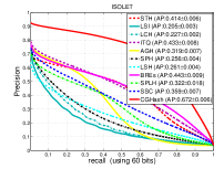
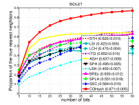
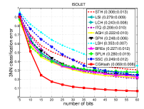
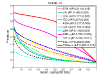
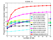
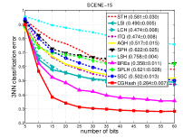
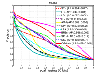
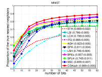
Experimental setup In order to evaluate the proposed column generation hashing method (referred to as CGHash), we have conducted a set of experiments on six benchmark datasets. To train data-dependent hash functions, each dataset is randomly split into a training subset and a testing subset. This training/testing split is repeated 5 times, and the average performance over these 5 trials is reported here.
In the experiments, the proposed hashing method is implemented by using the squared hinge loss function with the regularization norm (as shown in the supplementary file). Moreover, the triplets used for learning hash functions are generated in the same way as (Weinberger et al., 2006). Specifically, given a training sample, we select the nearest neighbors from its associated same-label training samples as relevant samples, and then choose the nearest neighbors from its associated different-label training samples as irrelevant samples ( for the SCENE-15 dataset and for the other datasets). The trade-off control factor is cross-validated. We found that, in a wide range, the trade-off control factor does not have a significant impact on the performance.
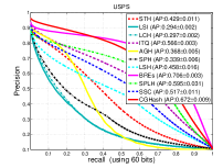
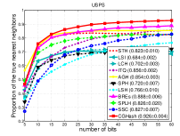
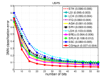
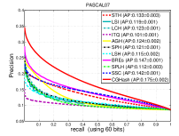
Competing methods To demonstrate the effectiveness of the proposed hashing method (CGHash), we compare with some other state-of-the-art hashing methods quantitatively. For simplicity, they are respectively referred to as LSH (Locality Sensitive Hashing (Andoni & Indyk, 2006)), SSC (Supervised Similarity Sensitive Coding (Torralba et al., 2008) as a modified version of (Shakhnarovich et al., 2003)), LSI (Latent Semantic Indexing (Deerwester et al., 1990)), LCH (Laplacian Co-Hashing (Zhang et al., 2010a)), SPH (Spectral Hashing (Weiss et al., 2008)), STH (Self-Taught hashing (Zhang et al., 2010b)), AGH (Anchor Graph Hashing (Liu et al., 2011)), BREs (Supervised Binary Reconstructive Embedding (Kulis & Darrell, 2009)), SPLH (Semi-Supervised Learning Hashing (Wang et al., 2012)), and ITQ (Iterative Quantization (Gong et al., 2012)). Making a comparison with the above competing methods can verify the effect of learning hashing functions and show the performance differences in the context of hashing methods.
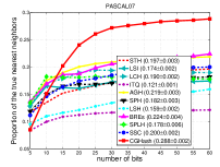
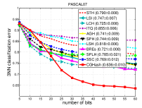
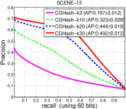
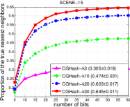
Evaluation criteria For a quantitative performance comparison, we introduce the following three evaluation criteria: i) precision-recall curve; ii) proportion of true neighbors in top- retrieval; and iii) -nearest-neighbor classification. In the experiments, the aforementioned retrieval performance scores are averaged over all test queries in the dataset. For i), the precision-recall curve is computed as follows: and . For ii), the proportion of true neighbors in top- retrieval is calculated as: . For iii), each test sample is classified by a majority voting in -nearest-neighbor classification.
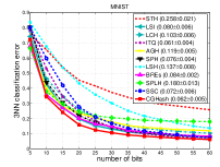
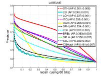
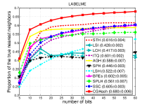
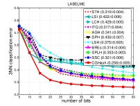
Quantitative comparison results Figs. 1–6 show the retrieval and classification performances of all the hashing methods using different code lengths on the six datasets. In each of these figures, we report quantitative comparison results of all the hashing methods in the following three aspects: 1) the average precision-recall performances using the maximum code length, and the average precisions together with standard deviations (as shown in the legend of each figure); 2) the average performances using different code lengths in the proportion of the true nearest neighbors with top-50 retrieval, and the average proportion results together with their standard deviations in the case of the maximum code length (as shown in the legend of each figure); and 3) the average -nearest-neighbor classification performances using different code lengths, and the average classification results together with their standard deviations in the case of the maximum code length (as shown in the legend of each figure).
From Figs. 1–6, we clearly see that the proposed CGHash obtains the larger areas under the precision-recall curves than the competing hashing methods. In addition, we observe that CGHash achieves the higher proportions of the true nearest neighbors with top-50 retrieval at most times. Moreover, it is seen that CGHash has lower classification errors than the competing methods in most cases.
Fig. 7 shows the retrieval and classification performances of the proposed CGHash using different values of on the SCENE-15 dataset. It is seen from Fig. 7 that in general the performance is improved as increases.
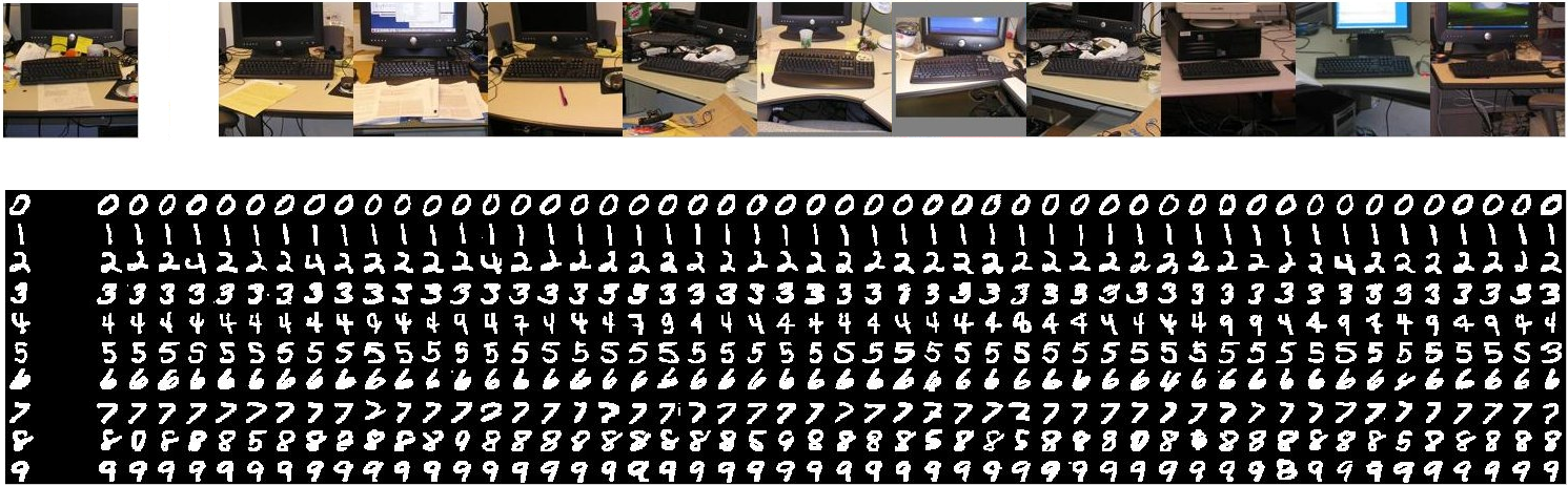
Besides, Fig. 8 shows two retrieval examples on the MNIST and LABELME datasets. From Fig. 8, we observe that CGHash obtains the visually accurate nearest-neighbor-search results.
Conclusion We have proposed a novel hashing method that is implemented using column generation-based convex optimization. By taking into account a set of constraints on the triplet-based relative ranking, the proposed hashing method is capable of learning compact hash codes. Such a set of constraints are incorporated into the large-margin learning framework. Hash functions are then learned iteratively using column generation. Experimental results on several datasets have shown that the proposed hashing method achieves improved performance compared with state-of-the-art hashing methods in nearest-neighbor classification, precision-recall, and proportion of true nearest neighbors retrieved.
This work is in part supported by ARC grants LP120200485 and FT120100969.
References
- Andoni & Indyk (2006) Andoni, A. and Indyk, P. Near-optimal hashing algorithms for approximate nearest neighbor in high dimensions. In Proc. IEEE Symp. Foundations of Computer Science, pp. 459–468, 2006.
- Baluja & Covell (2008) Baluja, S. and Covell, M. Learning to hash: forgiving hash functions and applications. Data Mining & Knowledge Discovery, 17(3):402–430, 2008.
- Boyd & Vandenberghe (2004) Boyd, S. and Vandenberghe, L. Convex Optimization. Cambridge University Press, 2004.
- Deerwester et al. (1990) Deerwester, S., Dumais, S.T., Furnas, G.W., Landauer, T.K., and Harshman, R. Indexing by latent semantic analysis. J. American Society for Information Science, 41(6):391–407, 1990.
- Demiriz et al. (2002) Demiriz, A., Bennett, K.P., and Shawe-Taylor, J. Linear programming boosting via column generation. Machine Learning, 46(1):225–254, 2002.
- Gong et al. (2012) Gong, Y., Lazebnik, S., Gordo, A., and Perronnin, F. Iterative quantization: a procrustean approach to learning binary codes for large-scale image retrieval. IEEE Trans. Pattern Analysis & Machine Intelligence, 2012.
- Korman & Avidan (2011) Korman, S. and Avidan, S. Coherency sensitive hashing. In Proc. Int. Conf. Computer Vision, pp. 1607–1614, 2011.
- Kulis & Darrell (2009) Kulis, B. and Darrell, T. Learning to hash with binary reconstructive embeddings. In Proc. Adv. Neural Information Process. Systems, 2009.
- Kulis & Grauman (2009) Kulis, B. and Grauman, K. Kernelized locality-sensitive hashing for scalable image search. In Proc. Int. Conf. Computer Vision, pp. 2130–2137, 2009.
- Li et al. (2013) Li, X., Lin, G., Shen, C., van den Hengel, A., and Dick, A. Supplementary document: Effectively learning hash functions using column generation. available at: http://cs.adelaide.edu.au/~chhshen/paper.html, 2013.
- Liu et al. (2011) Liu, W., Wang, J., Kumar, S., and Chang, S. F. Hashing with graphs. In Proc. Int. Conf. Machine Learning, 2011.
- Liu et al. (2012) Liu, W., Wang, J., Ji, R., Jiang, Y.G., and Chang, S.F. Supervised hashing with kernels. In Proc. IEEE Conf. Computer Vision & Pattern Recognition, 2012.
- Norouzi & Fleet (2011) Norouzi, M. and Fleet, D.J. Minimal loss hashing for compact binary codes. In Proc. Int. Conf. Machine Learning, 2011.
- Salakhutdinov & Hinton (2009) Salakhutdinov, R. and Hinton, G. Semantic hashing. Int. J. Approximate Reasoning, 50(7):969–978, 2009.
- Schultz & Joachims (2004) Schultz, M. and Joachims, T. Learning a distance metric from relative comparisons. In Proc. Adv. Neural Information Processing Systems, 2004.
- Shakhnarovich et al. (2003) Shakhnarovich, G., Viola, P., and Darrell, T. Fast pose estimation with parameter-sensitive hashing. In Proc. Int. Conf. Computer Vision, pp. 750–757, 2003.
- Shen et al. (2012) Shen, C., Kim, J., Wang, L., and van den Hengel, A. Positive semidefinite metric learning using boosting-like algorithms. J. Machine Learning Research, 13:1007–1036, 2012.
- Strecha et al. (2011) Strecha, C., Bronstein, A. M., Bronstein, M. M., and Fua, P. Ldahash: Improved matching with smaller descriptors. IEEE Trans. Pattern Analysis & Machine Intelligence, 2011.
- Torralba et al. (2008) Torralba, A., Fergus, R., and Weiss, Y. Small codes and large image databases for recognition. In Proc. IEEE Conf. Computer Vision & Pattern Recognition, pp. 1–8, 2008.
- Wang et al. (2012) Wang, J., Kumar, S., and Chang, S.F. Semi-supervised hashing for large scale search. IEEE Trans. Pattern Analysis & Machine Intelligence, 2012.
- Weinberger et al. (2006) Weinberger, K.Q., Blitzer, J., and Saul, L.K. Distance metric learning for large margin nearest neighbor classification. In Proc. Adv. Neural Information Processing Systems, 2006.
- Weiss et al. (2008) Weiss, Y., Torralba, A., and Fergus, R. Spectral hashing. In Proc. Adv. Neural Information Process. Systems, 2008.
- Zhang et al. (2010a) Zhang, D., Wang, J., Cai, D., and Lu, J. Laplacian co-hashing of terms and documents. In Proc. Eur. Conf. Information Retrieval, pp. 577–580, 2010a.
- Zhang et al. (2010b) Zhang, D., Wang, J., Cai, D., and Lu, J. Self-taught hashing for fast similarity search. In Proc. ACM SIGIR Conf., pp. 18–25, 2010b.
- Zhu et al. (1997) Zhu, C., Byrd, R. H., Lu, P., and Nocedal, J. Algorithm 778: L-BFGS-B: Fortran subroutines for large-scale bound-constrained optimization. ACM Trans. Math. Softw., 23(4):550–560, 1997.