Nature of the Roberge-Weiss transition end points in two-flavor lattice QCD with Wilson quarks
Abstract
We make simulations with 2 flavor Wilson fermions to investigate the nature of the end points of Roberge-Weiss (RW) first order phase transition lines. The simulations are carried out at 9 values of the hopping parameter ranging from 0.155 to 0.198 on different lattice spatial volume. The Binder cumulants, susceptibilities and reweighted distributions of the imaginary part of Polyakov loop are employed to determine the nature of the end points of RW transition lines. The simulations show that the RW end points are of first order at the values of in our simulations.
pacs:
12.38.Gc, 11.10.Wx, 11.15.Ha, 12.38.MhI INTRODUCTION
A full understanding of QCD phase diagram is of great importance theoretically and phenomenologically. The QCD phase diagram addresses which forms of nuclear matter exist at different finite temperature and baryon density, and whether there are bona fide phase transition separating them, thus it is essential for relativistic heavy ion collision experiments and astrophysics. QCD is a strongly interacting theory on the scales of a baryon mass and below, so non-perturbative calculations from the first principle are preferrable. Despite that substantial progress has been made with Monte Carlo simulations of lattice QCD at zero baryon density, the studies at nonzero baryon density are haunted by the “sign” problem, for example, see Ref. Kogut:2007mz . To date many indirect methods have been proposed to circumvent the sign problem, overviews with references to these methods can be found in Ref. Kogut:2007mz ; Schmidt:2006us . One of these methods consists of simulating QCD with the imaginary chemical potential for which the fermion determinant is positive deForcrand:2010he ; D'Elia:2009tm ; D'Elia:2009qz ; Nagata:2011yf ; Bonati:2010gi ; D'Elia:2007ke ; Wu:2006su ; deForcrand:2006pv ; deForcrand:2008vr . Full information can be obtained by using the imaginary chemical potential which allows for analytic continuation via truncated polynomials.
The phase structure of QCD with imaginary chemical potential not only deserves detailed investigations in its own right theoretically, but also has significant relevance to physics at zero or small real chemical potentialD'Elia:2009qz ; D'Elia:2007ke ; Bonati:2010gi ; Kouno:2009bm ; Sakai:2009vb ; deForcrand:2010he ; Aarts:2010ky ; Philipsen:2010rq ; Bonati:2012pe . QCD with imaginary chemical potential has a rich phase diagram as a function of imaginary chemical potential and quark masses.
In this paper, we present a study of phase structure of QCD at fixed imaginary chemical potential for QCD with Wilson quarks. The partition function including the imaginary chemical potential is
| (1) |
Roberge and Weiss made the essential work with the imaginary chemical potential Roberge:1986mm , they found that the partition function of QCD with imaginary chemical potential has two important symmetries, reflection symmetry in and periodicity in imaginary chemical potential,
| (2) |
| (3) |
The periodicity is smoothly realized in the low temperature, strong-coupling regime, whereas in the high temperature, weak-coupling regime, it is realized in a non-analytic way. At high temperature, the system undergoes a first order transition (RW transition) at critical values of the imaginary chemical potential Roberge:1986mm ; deForcrand:2002ci ; Lombardo between adjacent Z(3) sectors and these Z(3) sectors are characterized by the Polyakov loop. Thus the picture for the phase diagram is that repeats with a periodicity the first order transition line in the high temperature regime which necessarily ends at an end point at some temperature when the temperature is decreased sufficiently.
At these end points, there are evidence that the analytic continuation of deconfinement/chiral transition line from real chemical potential to imaginary chemical one meets the RW transition line. Recent numerical studies show that the RW transition line end points are triple points for small and heavy quark mass, and second order end points for intermediate quark masses. So there exist two tricritical points which separate the first order regime from the second one deForcrand:2010he ; D'Elia:2009qz ; Bonati:2010gi . Moreover, it is pointed out deForcrand:2010he ; Philipsen:2010rq ; Bonati:2012pe that the scaling behaviour at the tricritical points may shape the the critical line for real chemical potential, and subsequently, the line for real chemical potential is qualitatively consistent with the scenario suggested in Ref. deForcrand:2006pv ; deForcrand:2008vr which show that the first order region shrinks with the increasing real chemical potential.
Most of studies of finite temperature QCD have been performed using staggered fermion action or the improved versions Karsch ; Cheng:2006qk ; Cheng:2006aj ; Bernard:2004je ; Aoki:2006br ; Bernard:2007nm ; Aoki:2005vt , staggered fermion approach and Wilson fermion approach have their own advantages and disadvantages, for example, see Ref. Heller:2006ub . The KS fermion formalism preserves the U(1) chiral symmetry, whereas it needs a fourth root trick for one flavour which might lead to locality problem Bunk and phase ambiguities Golterman . On the contrary, Wilson fermions completely solve the species doubling problem, whereas it suffers from an explicit chiral symmetry breaking. The lattice simulation with Wilson fermions is more time-consuming than staggered fermions, it can provide complementary information and crosscheck to simulations with other actions and establish a better understanding of QCD phase diagram.
In this paper, we attempt to investigate the RW transition line end points by lattice QCD with two degenerate flavors of Wilson fermions. In Sec. II, we define the lattice action with imaginary chemical potential and the physical observables we calculate. Our simulation results are presented in Sec. III followed by discussions in Sec. IV.


II LATTICE FORMULATION WITH IMAGINARY CHEMICAL POTENTIAL
We consider the partition function of system with degenerate flavors of Wilson quarks with chemical potential on the lattice
| (4) | |||||
where is the gauge action, and is the quark action with the quark imaginary chemical potential . For , we use the standard one-plaquette action
| (5) |
where , and the plaquette variable is the ordered product of link variables around an elementary plaquette. For , we use the the standard Wilson action
| (6) |
where is the hopping parameter, related to the bare quark mass and lattice spacing by . The fermion matrix is
| (7) | |||||
We carry out simulations at . As it is pointed out that the system is invariant under the charge conjugation at , when is fixed Kouno:2009bm . But the -odd quantity is not invariant at under charge conjugation. When , is a smooth function of , so it is zero at . Whereas when , the two charge violating solutions cross each other at . Thus the charge symmetry is spontaneously broken there and the -odd quantity can be taken as order parameter . In this paper, we take the imaginary part of Polyakov loop as the order parameter.
The Polyakov loop is defined as the following:
| (8) |
here and in the following, is the spatial lattice volume. To simplify the notations, we use to represent the imaginary part of Polyakov loop , .
The susceptibility of imaginary part of Polyakov loop is defined as
| (9) |
which is expected to scale as: D'Elia:2009qz ; Bonati:2010gi
| (10) |
where is the reduced temperature , . This means that the curves at different lattice volume should collapse with the same curve when plotted against . In the following, we employ in place of . The critical exponents relevant to our study are collected in Table. 1 Bonati:2010gi ; Pelissetto:2000ek .
| 3D ising | 0.6301(4) | 1.2372(5) | 1.963 |
|---|---|---|---|
| tricritical | 1/2 | 1 | 2 |
| first order | 1/3 | 1 | 3 |
We also consider the Binder cumulant of the imaginary part of Polyakov loop which is defined as the following:
| (11) |
with . In the thermodynamic limit, takes on the values 3, 1.5, 1.604, 2 for crossover, first order triple point, 3D Ising and tricritical transitions, respectively. However, on finite spatial volumes, the steps are smeared out to continuous functions. In the vicinity of the RW transition line end points, is a function of and can be expanded as a series deForcrand:2010he ; Philipsen:2010rq ; Bonati:2012pe .
| (12) |
III MC SIMULATION RESULTS
In this section, we will present our results for simulating QCD with two degenerate flavors of Wilson fermions at finite temperature and imaginary chemical potential . Both the algorithm with a Metropolis accept/reject step and the algorithm are used Gottlieb:PRD:35:3972 . The simulations are performed on lattice with different spatial volume with temporal extent at . For each value, we carry out simulations on lattice of size , and for some values, lattice of size or/and are also used. Simulations are carried out with algorithm with a Metropolis accept/reject step with the acceptance rate ranging from , The other simulations are carried out in terms of algorithm with the molecular dynamics time step . Ref. Gottlieb:PRD:35:3972 pointed out that R-algorithm has errors of order , so the correct results of this algorithm consists of extrapolation to zero stepsize. However, in practice a short-cut without extrapolation is used. Recently, the exact RHMC algorithm is invented which also allows many improvements Clark:2002vz . In our simulation, is sufficiently smaller compared with the statistical errors of our simulations. There are 20 molecular steps for each trajectory. We generate 20,000 trajectories after 10,000 trajectories as warmup. Ten trajectories are carried out between measurements. We use the conjugate gradient method to evaluate the fermion matrix inversion.
On each lattice size, we make simulations at typically 4-6 different values. For fixed , there is transition in between the low temperature phase and the high temperature phase. In order to determine the RW transition line end point from the peak of susceptibilities, we use the data obtained through simulations at the 4-6 different values, and calculate susceptibilities at additional values, by employing the Ferrenberg-Swendsen reweighting method Ferrenberg:1989ui .
Let us first present the critical couplings on different spatial volume at different in Table. 2.
| 0.155 | |||||
|---|---|---|---|---|---|
| 0.160 | |||||
| 0.165 | |||||
| 0.168 | |||||
| 0.170 | |||||
| 0.175 | |||||
| 0.180 | |||||
| 0.190 | |||||
| 0.198 |
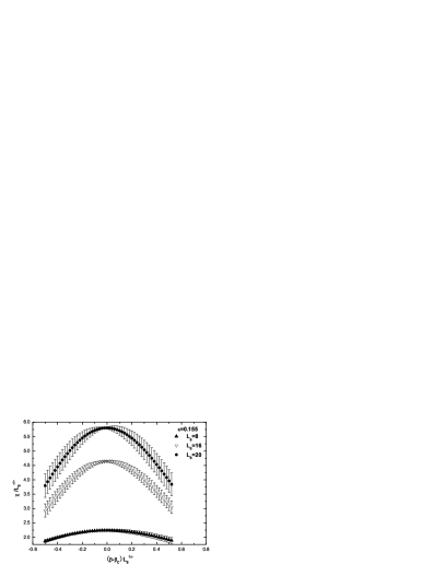
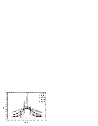
The presence of a first order phase transition at the end point of Roberge-Weiss transition line at can be found from the scaling behavior of the susceptibilities of the imaginary part of Polyakov loop presented in Fig. 1. From Fig. 1 we can find that the rescaling quantities plotted against does not fall on the same curve completely, whereas peaks of the rescaling quantities obviously exhibit scaling behavior which conforms to the first order transition. From Eq. (10), we can find that the index regulates the height of peaks while the index regulates the width of peaks. As a comparison, we also present the behavior according to the 3D Ising transition index in the right panel of Fig. 1 from which we can find that large deviation from the 3D Ising scaling behavior manifest clearly. At , similar observations of susceptibilities as those at can be found.
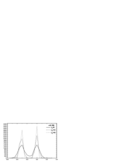
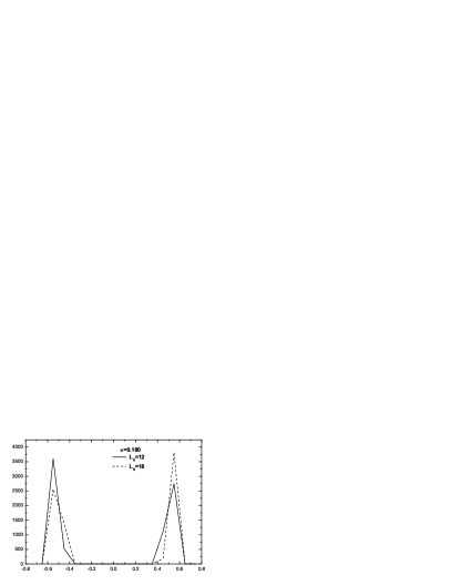
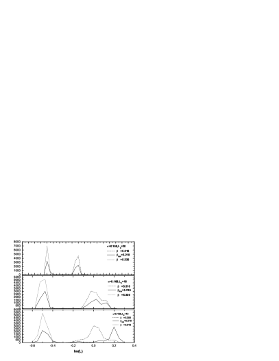
In Fig. 2, we present reweighted distributions of the imaginary part of Polyakov loop at the corresponding and two values on lattice size . On each lattice size, at , reweighted distribution of exhibits two-state signal, while, at and , reweighted distributions of do not exhibit two-state signal. At other values, reweighted distributions of the imaginary part of Polyakov loop at the corresponding , and on each lattice size have the same observations as those at . For clarity, we only present the result at in the following.
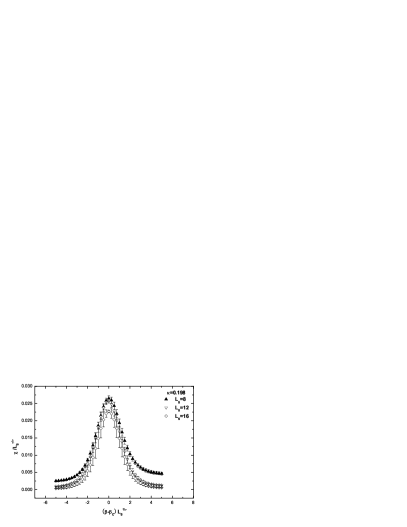
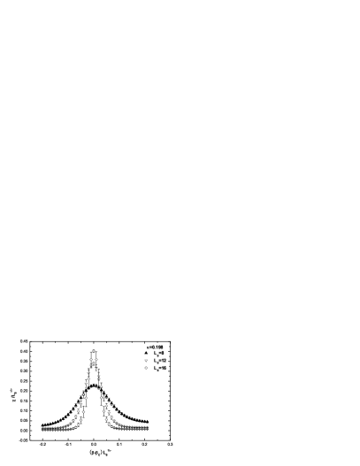
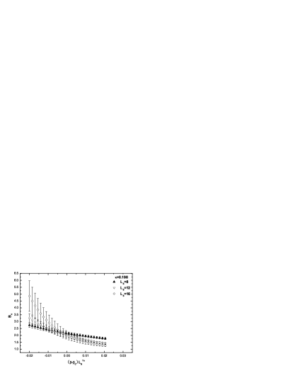
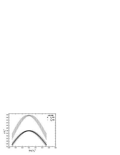
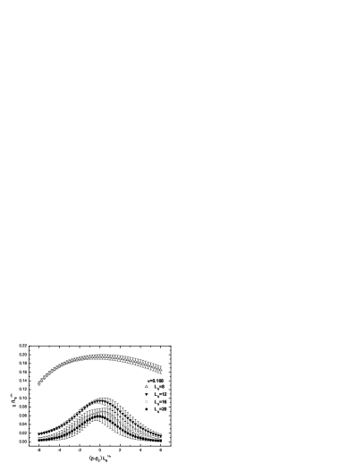
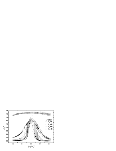
We also make simulations at , the results of simulations at are presented in Fig. 3, and Fig. 4. From the two upper panels of Fig. 3, we can find that the first order transition indexes are more suitable to describe the behavior than the 3D Ising ones. This situation can be made clearer when we look at the behavior depicted in down panels of Fig. 3 from which we can find that the quantities of Binder cumulant plotted against rescaling fall on the same curve completely. Note that from Eq. (11), the scaling behavior of Binder cumulants is governed by the critical index which also determines the width of peaks of the rescaling quantities . The fact that the value of for first order transition accounts for the width of peaks of better than the second order transition show that the transition is first order, and this situation is confirmed by the scaling behavior of Binder cumulant . We also present reweighted distribution of the imaginary part of Polyakov loop at at in Fig. 4 which exhibits two-state signal. At , similar observations as those at can be observed.
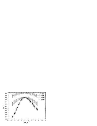
The results of simulations at are shown in Fig. 5. In view of the fact that large finite-size corrections are observed in simple spin models even when the transition is first order deForcrand:2010he ; Billoire:1992ke , we can find that the first order transition indexes perform much better than the second order transition ones. This observation can be enhanced from the reweighted distribution of the imaginary part of Polyakov loop presented in Fig. 6.


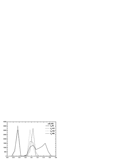

Comparing to the above results, it is difficult to determine the nature of RW transition line end points at results of which are presented in Fig. 7. However, when we look at the behavior at large lattice size presented in Fig. 7, it is a reasonable conclusion that the behavior of RW transition line end points at are of first order. This conclusion can be enhanced when we look at the reweighted distributions of at the end point at presented in Fig. 8. and reweighted distributions of at the corresponding , and on lattice size at presented in Fig. 9.


IV DISCUSSIONS
We have studied the nature of critical end points of Roberge-Weiss transition of two flavor lattice QCD with Wilson fermions. When , the imaginary part of Polayakov loop is the order parameter for studying the transition from low temperature phase to high temperature one. Within the imaginary chemical potential formulation, the partition function is periodic in imaginary chemical potential. The different Z(3) sectors are characterized by the phase of Polyakov loop. The Roberge-Weiss transition which occurs at is of first order in the high temperature phase, whereas it is of crossover in the low temperature phase.
Our simulations are carried out at 9 values of on different 3-4 spatial volumes. Our lattice is coarse. In Ref. Bitar:1993xd , the lattice spacing with 2 flavor Wilson fermions at is estimated to be . In Ref. Iwasaki:1996zt , the lattice spacing with 2 flavor Wilson fermions is estimated to be which is found almost independent of in the range of . In our simulations, varies roughly from to , thus, the lattice spacing is estimated to be .
In order to estimate the pseudo-scalar meson mass , the vector meson mass and ratios at our simulation points, we use the data in Table II in Ref. Bitar:1990si . By using the standard quark and gauge action, Bitar et al. studied hadron thermodynamics with Wilson fermions on lattice and calculated the zero temperature hadron mass on lattice with dynamical fermions. We compile their results and present in the following: at , , at , , at , , and at , . Using the lattice spacing estimated in the above, we find that at , , at , . Comparing the values of at simulation points in Ref. Bitar:1990si with ours. we can roughly estimate the pseudo-scalar meson mass . Using the estimated lattice spacing, we can estimate that Roberge-Weiss transition point temperature varies from in our simualtions.
We consider the peak behaviour, reweighted distribution and Binder cumulant of order parameter around the critical end point , At , the three observables’ behaviour show that transition at the end point is of first order which means the end point is a triple point. At , the peak behavior at the end point are more consistent with that of transition of a triple point than that of 3D Ising transition behaviour. Similar observations can be observed at .
At , it becomes difficult to discern the peak behavior between 3D Ising transition class and triple point, however, when we look at the peak behavior at large lattice size, it is a reasonable conclusion that the behavior of RW transition line end points are of first order. This conclusion is enhanced by the reweighted distribution of order parameter.
We also fit Eq. (12) to the calculated Binder cumulant data to extract the value of critical index . At , , respectively, and these values conform to first order transition.
In Ref. Aarts:2010ky , the locations of triple points are determined. In Ref. D'Elia:2009qz ; Bonati:2010gi and Ref. deForcrand:2010he , the simulations with staggered fermions show that phase diagram of two flavor and three flavor QCD at imaginary chemical potential are characterized by two tricritical points, respectively. Our simulations have no evidence that shows the existence of tricritical points separating second order region from the first order region. Considering these results, our investigation requires further extensive numerical simulations which extend to a larger range of quark mass region. This work is under progress.
Acknowledgements.
We thank the referee for the comments very much. We modify the MILC collaboration’s public codeMilc to simulate the theory at imaginary chemical potential. This work is supported by the National Science Foundation of China (NSFC) under Grants No. 11105033. The work was carried out at National Supercomputer Center in Tianjin,and the calculations were performed on TianHe-1A.References
- (1) J. B. Kogut and D. K. Sinclair, Phys. Rev. D 77, 114503 (2008) [arXiv:0712.2625 [hep-lat]].
- (2) C. Schmidt, PoS LAT 2006, 021 (2006) [hep-lat/0610116].
- (3) P. de Forcrand and O. Philipsen, Phys. Rev. Lett. 105, 152001 (2010) [arXiv:1004.3144 [hep-lat]].
- (4) M. D’Elia and F. Sanfilippo, Phys. Rev. D 80, 111501 (2009) [arXiv:0909.0254 [hep-lat]].
- (5) C. Bonati, G. Cossu, M. D’Elia and F. Sanfilippo, Phys. Rev. D 83, 054505 (2011) [arXiv:1011.4515 [hep-lat]].
- (6) M. D’Elia, F. Di Renzo and M. P. Lombardo, Phys. Rev. D 76, 114509 (2007) [arXiv:0705.3814 [hep-lat]].
- (7) K. Nagata and A. Nakamura, Phys. Rev. D 83, 114507 (2011) [arXiv:1104.2142 [hep-lat]].
- (8) M. D’Elia and F. Sanfilippo, Phys. Rev. D 80, 014502 (2009) [arXiv:0904.1400 [hep-lat]].
- (9) P. de Forcrand and O. Philipsen, JHEP 0701, 077 (2007) [hep-lat/0607017].
- (10) P. de Forcrand and O. Philipsen, JHEP 0811, 012 (2008) [arXiv:0808.1096 [hep-lat]].
- (11) L. -K. Wu, X. -Q. Luo and H. -S. Chen, Phys. Rev. D 76, 034505 (2007) [hep-lat/0611035].
- (12) Y. Sakai, H. Kouno and M. Yahiro, J. Phys. G 37, 105007 (2010) [arXiv:0908.3088 [hep-ph]].
- (13) G. Aarts, S. P. Kumar and J. Rafferty, JHEP 1007, 056 (2010) [arXiv:1005.2947 [hep-th]].
- (14) H. Kouno, Y. Sakai, K. Kashiwa and M. Yahiro, J. Phys. G 36, 115010 (2009) [arXiv:0904.0925 [hep-ph]].
- (15) O. Philipsen and P. de Forcrand, PoS LATTICE 2010, 211 (2010) [arXiv:1011.0291 [hep-lat]].
- (16) C. Bonati, P. de Forcrand, M. D’Elia, O. Philipsen and F. Sanfilippo, PoS LATTICE 2011, 189 (2011) [arXiv:1201.2769 [hep-lat]].
- (17) A. Roberge and N. Weiss, Nucl. Phys. B 275, 734 (1986).
- (18) P. de Forcrand and O. Philipsen, Nucl. Phys. B 642, 290 (2002).
- (19) M. D’Elia and M. -P. Lombardo, Phys. Rev. D 67, 014505 (2003) [hep-lat/0209146].
- (20) F. Karsch, E. Laermann and A. Peikert, Nucl. Phys. B 605, 579 (2001) [hep-lat/0012023].
- (21) Y. Aoki, Z. Fodor, S. D. Katz and K. K. Szabo, JHEP 0601, 089 (2006) [hep-lat/0510084].
- (22) M. Cheng, et al., Phys. Rev. D 74, 054507 (2006) [hep-lat/0608013].
- (23) Y. Aoki, Z. Fodor, S. D. Katz and K. K. Szabo, Phys. Lett. B 643, 46 (2006) [hep-lat/0609068].
- (24) M. Cheng, N. H. Christ, M. A. Clark, J. van der Heide, C. Jung, F. Karsch, O. Kaczmarek and E. Laermann et al., Phys. Rev. D 75, 034506 (2007) [hep-lat/0612001].
- (25) C. Bernard et al. [MILC Collaboration], Phys. Rev. D 71, 034504 (2005) [arXiv:hep-lat/0405029].
- (26) C. Bernard, et al. Phys. Rev. D 77, 014503 (2008) [arXiv:0710.1330 [hep-lat]].
- (27) U. M. Heller, PoS LAT 2006, 011 (2006) [hep-lat/0610114].
- (28) B. Bunk, M. Della Morte, K. Jansen and F. Knechtli, Nucl. Phys. B 697, 343 (2004).
- (29) M. Golterman, Y. Shamir and B. Svetitsky, Phys. Rev. D 74, 071501(R) (2006).
- (30) A. Pelissetto and E. Vicari, Phys. Rept. 368, 549 (2002) [cond-mat/0012164].
- (31) S. Gottlieb, W. Liu, D. Toussaint, R. L. Renken and R. L. Sugar, Phys. Rev. D 35, 3972 (1987).
- (32) M. A. Clark, B. Joo and A. D. Kennedy, Nucl. Phys. Proc. Suppl. 119, 1015 (2003) [hep-lat/0209035]; M. A. Clark and A. D. Kennedy, Nucl. Phys. Proc. Suppl. 129, 850 (2004) [hep-lat/0309084]; M. A. Clark, A. D. Kennedy and Z. Sroczynski, Nucl. Phys. Proc. Suppl. 140, 835 (2005) [hep-lat/0409133].
- (33) A. M. Ferrenberg and R. H. Swendsen, Phys. Rev. Lett. 63, 1195 (1989).
- (34) A. Billoire, T. Neuhaus and B. Berg, Nucl. Phys. B 396, 779 (1993) [hep-lat/9211014].
- (35) K. M. Bitar, T. A. DeGrand, R. Edwards, S. A. Gottlieb, U. M. Heller, A. D. Kennedy, J. B. Kogut and A. Krasnitz et al., Phys. Rev. D 49, 3546 (1994) [hep-lat/9309011].
- (36) Y. Iwasaki, K. Kanaya, S. Kaya, S. Sakai and T. Yoshie, Phys. Rev. D 54, 7010 (1996) [hep-lat/9605030].
- (37) K. M. Bitar et al., Phys. Rev. D 43, 2396 (1991).
- (38) http://physics.utah.edu/~detar/milc/