The Meaning and Consequences of Star Formation Criteria in Galaxy Models with Resolved Stellar Feedback

Abstract

We consider the effects of different criteria for determining where stars will form in gas on galactic scales, in simulations with high (1 pc) resolution, with explicitly resolved physics of GMC formation and destruction and stellar feedback from supernovae, radiation pressure, stellar winds, and photo-heating. We compare: (1) a self-gravity criterion (based on the local virial parameter and the assumption that self-gravitating gas collapses to high density in a single free-fall time), (2) a fixed density threshold, (3) a molecular-gas law, (4) a temperature threshold, (5) a requirement that the gas be Jeans-unstable, (6) a criteria that cooling times be shorter than dynamical times, and (7) a convergent-flow criterion. We consider all of these in both a MW-like and high-density (starburst or high-redshift) galaxy. With feedback present, all models produce identical integrated star formation rates (SFRs), in good agreement with the Kennicutt relation; without feedback all produce orders-of-magnitude excessive SFRs. This is totally dependent on feedback and independent of the SF law, even if the “local” collapse efficiency is $100\%$. However, the predicted spatial and density distribution depend strongly on the SF criteria. Because cooling rates are generally fast within galaxy disks, and gas is turbulent, criteria (4)-(7) are very “weak” and spread the SF uniformly over most of the disk (down to densities $n\sim 0.01-0.1\,{\rm cm^{-3}}$). A molecular criterion (3) localizes to slightly higher densities, but still a wide range; for metallicity near solar, it is almost identical to a fixed density threshold at $n\sim 1\,{\rm cm^{-3}}$ (well below the mean density in the central MW or starburst systems). A fixed density threshold (2) can always select the highest resolved densities, but must be adjusted both for simulation resolution and individual galaxy properties – the same threshold that works well in a MW-like simulation will select nearly all gas in a starburst. Binding criteria (1) tend to adaptively select the largest local over-densities, independent of galaxy model or resolution, and automatically predict clustered star formation. We argue that this SF model (possible with other secondary criteria) is most physically-motivated and presents significant numerical advantages in simulations with a large dynamic range.

1 Introduction

Modeling star formation accurately is critical for any simulation of galaxy formation. However, cosmological and galaxy-scale simulations still cannot hope to resolve the spatial and density scales on which star formation actually occurs. As a result, simple “recipes” must be applied. For example, models typically impose some “local Schmidt law,” where gas forms stars at a rate that scales as some power of the density; if the SFR per local free-fall time $t_{\rm ff}\propto 1/\sqrt{G\rho}$ were constant, this would be $\dot{\rho}_{\ast}\propto\rho/t_{\rm ff}\propto\rho^{1.5}$, although in principle any other parameters can be used.

Usually, applying these models alone would artificially spread star formation among all the gas in the simulation, even cosmologically pristine material at high temperatures. So some additional criteria or restrictions must be included. Most commonly, this amounts to a simple density threshold: $n\gtrsim 0.1\,{\rm cm^{-3}}$ in many cosmological simulations. This is not to say such low-density material directly forms stars: rather, this corresponds crudely to densities where the thermal instability sets in, so some un-resolved fraction of the material (which goes into the sub-grid scaling above) will be able to form stars. Other common requirements include restricting star formation to gas which is below some temperature, or Jeans unstable, or in convergent flows, or which has a short cooling time. Recently, various studies have considered molecular criteria: using some combination of density and metallicity to estimate a sub-grid molecular gas fraction and restricting star formation to the “molecular” gas (Robertson & Kravtsov, 2008; Kuhlen et al., 2012).

These criteria are not trivial. Star formation is observed to be highly clustered under essentially all conditions (Lada & Lada, 2003, and references therein), and without some criteria such as those above, this is not captured in simulations. This does not just mean that stars are forming in the wrong places. “Smearing out” star formation over the disk dramatically suppresses the effects of stellar feedback (Governato et al., 2010). Massive star clusters allow for e.g. overlapping SNe “bubbles” that can expand much more efficiently than individual SNe remnants. They also concentrate feedback “where it is needed,” i.e. it preferentially acts in the dense, star-forming gas. Strong radiation pressure effects arise when photons are trapped in optical thick regions around embedded clusters (Hopkins et al., 2011). And spreading out star formation leads to spurious geometric cancellation between feedback sources. Without a sufficiently strict minimum SF criterion, the ability of the gas to form realistic phase structure (Saitoh et al., 2008), or blow winds that regulate its baryon content (Governato et al., 2010) and form realistic disks (Pontzen & Governato, 2012; Governato et al., 2004) can be fundamentally altered.

Unfortunately, in practice the physical interpretation of these criteria often depends both on the resolved dynamic range of the simulation and on the mean properties of the galaxies being simulated, and to obtain similar results they must be numerically adjusted accordingly.

However, it is increasingly clear that the ISM is governed by super-sonic turbulence over a wide range of scales. Consider, then, a locally self-gravitating region of the ISM “supported” by turbulence. In the absence of some feedback disrupting it or “pumping” the dispersion, the turbulent support will be damped in a single crossing time; as a result the region will collapse to arbitrarily high densities in about one free-fall time. This is true even if the energy of contraction maintains a constant virial equilibrium at each radius (Hopkins, 2013). At sufficiently high densities, eventually all of the above criteria must be met; so long as the SFR increases with density, eventually an order-unity fraction of the gas will be consumed into stars. So – in the absence of some self-regulation – the time-averaged SFR should be $\dot{\rho}_{\ast}\approx\rho/t_{\rm collapse}\sim\rho/t_{\rm ff}$ regardless of the “true” local star formation criteria/law. This is precisely what is seen in detailed simulations of turbulent media, in the absence of “pumping” to unbind collapsing regions (Ballesteros-Paredes et al., 2011; Padoan & Nordlund, 2011; Padoan et al., 2012).

We stress that this does not mean the total SFR, even within a dense parcel of gas, will actually be as large as $\rho_{\rm gas}/t_{\rm ff}$. If feedback is present, it can self-regulate. As soon as some gas turns into stars, feedback can act and disrupt the bound material, terminating the star formation locally and suppressing nearby star formation even in the dense gas. In such a model, however, the “net” efficiency is actually predicted self-consistently from the feedback model, rather than imposed by the sub-grid model (by, say, forcing some by-hand low normalization of $\dot{\rho_{\ast}}(\rho)$.

Of course, if a simulation resolves a bound region, then this collapse will be followed self-consistently. What we require is a mechanism to treat further collapse, where it would occur, below our resolution limit. In this paper, we propose a simple adaptive self-gravity criterion for star formation in galaxy-scale and cosmological simulations, motivated by the numerical simulations above. We compare it to other common criteria in the literature, and examine the implications for the equilibrium SFRs and both the predicted spatial and density distributions of SF in different galaxy environments.

2 A Simple Self-Gravity Criterion

On some scale $\delta r$, self-gravity requires $\sigma_{\rm eff}^{2}+c_{s}^{2}<\beta\,G\,M(<\delta r)/\delta r$, where $\sigma_{\rm eff}$ includes the contributions from both rotational and random motions and $\beta$ is an appropriate constant that depends on the internal structure in $\delta r$. In practice the gas of interest is always highly super-sonic in our simulations (and in observations), so we can ignore the $c_{s}$ term here. We then obtain the usual virial parameter

$$\alpha\equiv\sigma_{\rm eff}^{2}\,\delta r/\beta\,G\,M(<\delta r).$$ (1)

To determine local binding, we wish to describe $\alpha$ in the limit where $\delta r$ is small. Then $M(<\delta r)=(4\pi/3)\,\bar{\rho}\,\delta r^{3}$ where $\bar{\rho}$ is the average density in $\delta r$, and $\sigma_{\rm eff}\rightarrow\frac{\delta{\bf v}}{\delta{\bf r}}\,\delta r$, or more formally

$$\sigma_{\rm eff}^{2}=\beta_{v}\,{\bigl{(}}|\nabla\cdot{\bf v}|^{2}+|\nabla\times{\bf v}|^{2}{\bigr{)}}\,\delta r^{2}\equiv{\Bigl{(}}\frac{\delta\,v}{\delta\,r}{\Bigr{)}}^{2}\,\delta r^{2}$$ (2)

Here the $\nabla\cdot{\bf v}$ term accounts for the local radial velocity dispersion and inflow/outflow motions, while the $\nabla\times{\bf v}$ term accounts for internal rotational/shear and tangential dispersion. The $\beta_{v}$ term depends on the internal structure again but is close to unity.

Combining these terms, we can derive the formally resolution-independent criterion:

$$\alpha\equiv\frac{\beta^{\prime}}{2}\,\frac{|\nabla\cdot{\bf v}|^{2}+|\nabla\times{\bf v}|^{2}}{G\,\rho}<1$$ (3)

where $\beta^{\prime}\approx 1/2$ collects the order-unity terms above. This pre-factor depends on the internal mass profile and velocity structure, but only weakly: for e..g a Plummer sphere or Hernquist (1990) mass distribution with pure isotropic, rotationally supported, or constant velocity gradient orbits the range is $\beta^{\prime}\approx 0.5-0.6$.

This criterion is well-behaved in the local limit and does not explicitly depend on any numerical parameters of the simulation (spatial or mass resolution), nor does it require inserting any “ad hoc” threshold or normalization criterion. Because it depends only on the local velocity gradient and density, it is trivial to implement in either Lagrangian (SPH) or Eulerian (grid) codes (as compared to an explicit evaluation of the binding criterion over some resolved scale length, which requires a neighbor search, and can be prohibitively expensive in certain situations).

Implicitly, the velocity gradients and average density are always evaluated at the scale of the resolution limit. If going to higher resolution would change these quantities, then of course the criterion would give a different result (but as a consequence of the physical, not numerical, difference).

3 The Simulations

The simulations used here are described in detail in Hopkins et al. (2011) (hereafter Paper I; see § 2 & Tables 1-3) and Hopkins et al. (2012b) (Paper II; § 2). We briefly summarize the most important properties here. The simulations were performed with the parallel TreeSPH code GADGET-3 (Springel, 2005). They include stars, dark matter, and gas, with cooling, shocks, star formation, and stellar feedback.

3.1 Star Formation Criteria

Star formation is allowed only in gas that meets some set of criteria, for example in density or temperature. Within the gas that is flagged as “star forming,” our standard model assumes $\dot{\rho}_{\ast}=\epsilon\,{\rho}/{t_{\rm ff}}$ where $t_{\rm ff}$ is the free-fall time and $\epsilon$ is some efficiency. Unless otherwise specified, we set $\epsilon=0.015$, to match the average observed efficiency in dense gas (e.g. Krumholz & Tan, 2007, and references therein).

There are several criteria that can be imposed to determine the gas allowed to form stars:

(1) Self-Gravity: We require a region be locally self-gravitating as described in § 2, i.e. $\alpha<1$. But these regions are assumed to collapse in a single free-fall time, so $\epsilon=1$ (this approximates the results in individual cloud simulations of Padoan et al. 2012).

(2) Density: Star formation is allowed above a simple density threshold $n>n_{0}$, where we adopt $n_{0}=100\,{\rm cm^{-3}}$ to ensure this selects only over-dense gas inside of typical GMCs.

(3) Molecular Gas: We calculate the molecular fraction $f_{\rm H_{2}}$ of all gas as a function of the local column density and metallicity following Krumholz & Gnedin (2011) and allow star formation only from the molecular gas (i.e. multiply $\epsilon$ by $f_{\rm H_{2}}$).

(4) Temperature: We allow star formation only below a minimum temperature $T<T_{\rm min}$. Here we adopt $T_{\rm min}=100\,K$, (chosen to approach the minimum temperatures the simulation can resolve). At these temperatures, we expect this to be very similar to criterion (2).

(5) Jeans Instability: We require the gas be locally Jeans-unstable below the resolution limit: $c_{s}<h_{\rm sml}\,\sqrt{4\pi\,G\,\rho}$ ($h_{\rm sml}$ is the SPH smoothing length). Given the Lagrangian nature of the simulations, this translates to a temperature $T\lesssim 100\,{\rm K}\,(m_{i}/300\,M_{\sun})/(h_{\rm sml}/{\rm 10pc})$ where $m_{i}$ is the particle mass.

(6) Converging Flows: Star formation is allowed only in convergent flows, i.e. where $\nabla\cdot{\bf v}<0$.

(7) Rapid Cooling: We allow star formation only in regions where the cooling time is less than the dynamical time, $t_{\rm cool}<1/\sqrt{G\,\rho}$.

3.2 Cooling & Feedback

Gas follows an atomic cooling curve with additional fine-structure cooling to $\sim 10\,$K. At all the scales we resolve, the cooling time in dense gas tends to be much shorter than the dynamical time for any temperatures $T\gtrsim 10^{4}\,$K where the thermal pressure would be significant, and the minimum resolved scales are significantly larger than the sonic length. As a result, varying the cooling curve shape, magnitude, or metallicity dependence within an order of magnitude has no significant effect on any of our conclusions.

Stellar feedback is included, from a variety of mechanisms.

(1) Local Momentum-Driven Winds from Radiation Pressure, Supernovae, & Stellar Winds: Gas within a GMC (identified with an on-the-fly friends-of-friends algorithm) receives a direct momentum flux from the stars in that cluster/clump. The momentum flux is $\dot{P}=\dot{P}_{\rm SNe}+\dot{P}_{\rm w}+\dot{P}_{\rm rad}$, where the separate terms represent the direct momentum flux of SNe ejecta, stellar winds, and radiation pressure. The first two are directly tabulated for a single stellar population as a function of age and metallicity $Z$ and the flux is directed away from the stellar center. Because this is interior to clouds, the systems are always optically thick, so the latter is approximately $\dot{P}_{\rm rad}\approx(1+\tau_{\rm IR})\,L_{\rm incident}/c$, where $1+\tau_{\rm IR}=1+\Sigma_{\rm gas}\,\kappa_{\rm IR}$ accounts for the absorption of the initial UV/optical flux and multiple scatterings of the IR flux if the region is optically thick in the IR (with $\Sigma_{\rm gas}$ calculated for each particle).

(2) Supernova Shock-Heating: Gas shocked by supernovae can be heated to high temperatures. We tabulate the SNe Type-I and Type-II rates from Mannucci et al. (2006) and STARBURST99, respectively, as a function of age and metallicity for all star particles and stochastically determine at each timestep if a SNe occurs. If so, the appropriate mechanical luminosity is injected as thermal energy in the gas within a smoothing length of the star particle.

(3) Gas Recycling and Shock-Heating in Stellar Winds: Gas mass is returned to the ISM from stellar evolution, at a rate tabulated from SNe and stellar mass loss (integrated fraction $\approx 0.3$). The SNe heating is described above. Similarly, stellar winds are assumed to shock locally and inject the appropriate tabulated mechanical luminosity $L(t,\,Z)$ as a function of age and metallicity into the gas within a smoothing length.

(4) Photo-Heating of HII Regions and Photo-Electric Heating: We also tabulate the rate of production of ionizing photons for each star particle; moving radially outwards from the star, we then ionize each neutral gas particle (using its density and state to determine the necessary photon number) until the photon budget is exhausted. Ionized gas is maintained at a minimum $\sim 10^{4}\,$K until it falls outside an HII region. Photo-electric heating is followed in a similar manner using the heating rates from Wolfire et al. (1995).

(5) Long-Range Radiation Pressure: Photons which escape the local GMC (not accounted for in (1)) can be absorbed at larger radii. Knowing the intrinsic SED of each star particle, we attenuate integrating the local gas density and gradients to convergence. The resulting “escaped” SED gives a flux that propagates to large distances, and can be treated in the same manner as the gravity tree to give the local net incident flux on a gas particle. The local absorption is then calculated integrating over a frequency-dependent opacity that scales with metallicity, and the radiation pressure force is imparted.

Details and numerical tests of these models are discussed in Paper II. All energy, mass, and momentum-injection rates are taken as-is from the stellar population models in STARBURST99, assuming a Kroupa (2002) IMF, without any free parameters. Subtle variations in the implementation do not make significant differences to our conclusions. Most important, we do not “turn off” or otherwise alter any of the cooling or hydrodynamics of the gas.

3.3 Galaxy Models

We implement the model in two distinct initial disk models, chosen to span a wide range in ISM densities. Each has a bulge, stellar and gaseous disk, halo, and central BH (although to isolate the role of stellar feedback, models for BH growth and feedback are disabled). At our standard resolution, each model has $\sim 0.3-1\times 10^{8}$ total particles, giving particle masses of $\sim 500\,M_{\sun}$ and typical $\sim 5$ pc smoothing lengths in the dense gas, and are run for a few orbital times each. The disk models include:

(1) MW: a MW-like galaxy, with with baryonic mass $M_{\rm bar}=7.1\times 10^{10}\,M_{\sun}$ (gas $m_{g}=0.9\times 10^{10}\,M_{\sun}$, bulge $M_{b}=1.5\times 10^{10}\,M_{\sun}$, the remainder in a stellar disk $m_{d}$) and halo mass $M_{\rm halo}=1.6\times 10^{12}\,M_{\sun}$. The gas (stellar) scale length is $h_{g}=6.0\,$kpc ($h_{d}=3.0$). At standard resolution, gas particles and new stars have mass $m\approx 500\,M_{\sun}$ and the force softening $\epsilon\approx 4\,$pc.

(2) HiZ/Starburst: a massive starburst disk with densities typical of the central couple kpc in low-$z$ galaxy mergers, or the larger-scale ISM in star-forming galaxies at $z\sim 2-4$. Here $M_{\rm halo}=1.4\times 10^{12}\,M_{\sun}$ and baryonic $(M_{\rm bar},\,m_{b},\,m_{d},\,m_{g})=(10.7,\,0.7,\,3,\,7)\times 10^{10}\,M_{\sun}$ with scale-lengths $(h_{d},\,h_{g})=(1.6,\,3.2)\,{\rm kpc}$.

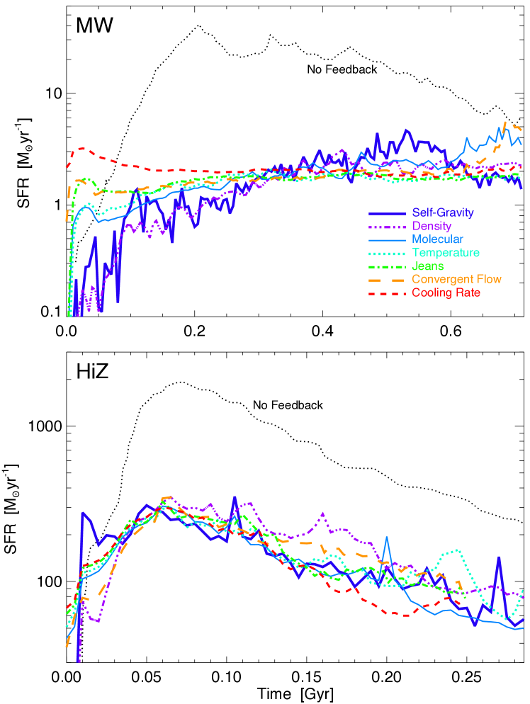
Figure 1: SFR vs. time for the simulations with different star formation prescriptions (as labeled), in the MW-like (top) and starburst/HiZ (bottom) disk models. The SF prescription has no effect on the actual SFRs (model differences, after the first couple dynamical times where non-equilibrium effects appear, are consistent with random variation). With realistic stellar feedback models, the SFR is entirely set by feedback (the mass in young stars needed to prevent runaway collapse). With no feedback, SF efficiencies are extremely large (SFRs much larger than observed); with feedback, the SFRs agree well with observations in both models. In particular, despite having an instantaneous, local efficiency $\epsilon=1$ in bound clouds, the actual average efficiency $\langle\epsilon\rangle$ of the “self-gravity” model is a realistic $\sim 1-5\%$.

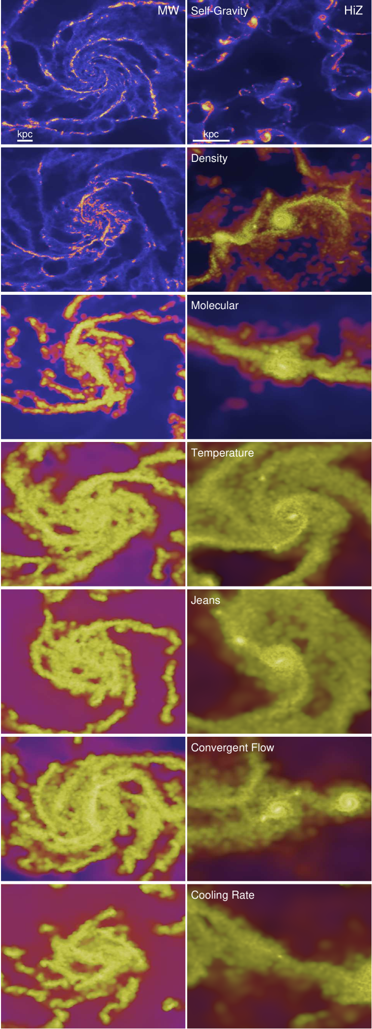
Figure 2: Gas surface density (intensity), with star-forming regions color-coded as red-yellow (with increasing specific SFR). The distribution of SF varies with SF law. Local binding criteria select locally over-dense regions in all cases. A fixed density threshold works well for most of the MW disk, but fails in the central, high-$\rho$ regions of the HiZ model (where the mean density is above-threshold). A molecular law works reasonably well in the outer regions of the MW model, but “smears” SF among a much wider range of gas in spiral arms; in the HiZ/starburst nucleus model it identifies all gas as molecular. Temperature, Jeans stability, cooling rate, and convergent-flow criteria select gas at nearly all densities.

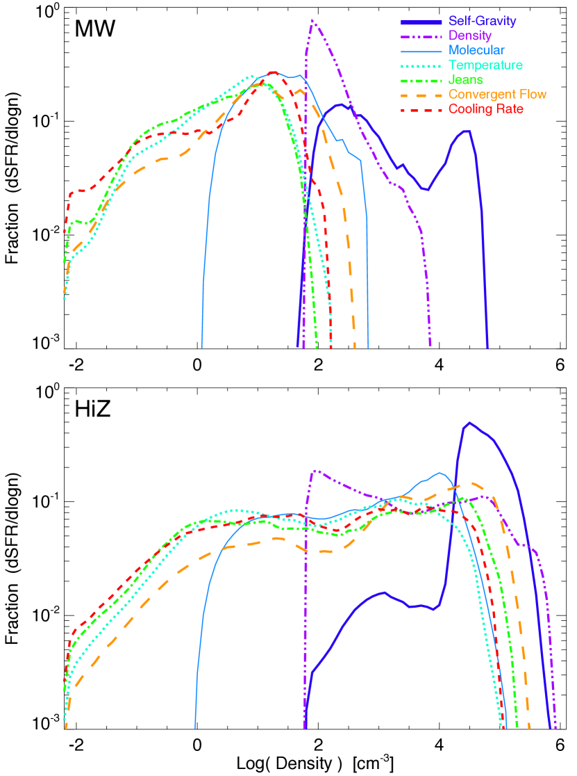
Figure 3: SFR-weighted density distribution for the simulations with different star formation prescriptions (labeled) in the MW-like (top) and starburst/HiZ (bottom) disk models. The self-gravity criterion identifies the most dense regions. A fixed-density threshold simulation is dominated by SF near the threshold, which is much lower than the maximum densities in the HiZ model. A molecular criterion effectively corresponds to a much lower threshold; for the metallicities here $\approx 1\,{\rm cm^{-3}}$. The other criteria spread the SF across almost all the gas, even at very low densities.

4 Results & Discussion

Figure 1 shows the total SFR versus time for the models, with feedback enabled and disabled. We immediately see that the total SFR, hence the net SF efficiency, is almost totally independent of the SF criteria. However, it depends dramatically on feedback. With feedback on, the global SFR is $\dot{M}_{\ast}\sim 0.02\,M_{\rm gas}/t_{\rm dyn}$, in agreement with observations. Without feedback, it is $\dot{M}_{\ast}\sim 0.5\,M_{\rm gas}/t_{\rm dyn}$. Regardless of how mass turns into stars, a certain feedback strength, hence mass in young stars, is needed to inject enough momentum to offset dissipation and prevent runaway collapse. Because cooling is rapid, the galaxy can always find a way to get “enough” gas to the relevant densities/temperatures/binding criteria – at which point the SFR is a function of feedback efficiency alone. This is discussed in much greater detail in Paper I, where we show that, for example, changing the local SF law (efficiencies, power-law indices, or density thresholds) makes no difference here, but changing the feedback strength directly changes the net efficiency. Without explicit feedback models, a local SF model that turned self-gravitating gas into stars with an efficiency $\sim 1$ would grossly over-produce observed SFRs; however, once feedback is included, the mean SF efficiency even in dense gas is a self-regulating quantity and we can safely consider such a prescription.

The SF criteria does, however, affect the the spatial and density distribution of star formation in each model, shown in Figures 2-3. With arbitrarily high resolution, we would ideally want all the star formation to be highly spatially clustered, and concentrated in absolute densities of $\gtrsim 10^{6}\,{\rm cm^{-3}}$. Resolution limits mean this cannot be realized; the “next-best” aim of these star formation criteria is to identify the highest local over densities and highest resolvable densities, which will contain sub-regions that collapse further, and associate star formation with those regions.

Our proposed self-gravity criterion (1) adaptively selects the over-dense regions in all galaxy models, giving a realistic “clumpy” and clustered morphology for the star formation. In the HiZ model in particular, it is able to associate star formation with a number of small sub-clumps in the central regions, with densities $\gtrsim 10^{4}\,{\rm cm^{-3}}$. (Note that the apparent “bimodality” here is artificial, caused by a bottleneck at the highest densities allowed by our numerical resolution).

A pure density criterion (2) works well when the threshold density is much larger than the background mean; however, it qualitatively changes character when the threshold falls below the mean density (the central regions of the HiZ model). Then, obviously, the SF becomes “smeared” uniformly across all the gas, defeating the purpose of a density threshold in the first place. This is clear in the morphology in Fig. 2, where the “clumps” previously evident have been largely “smeared out” by more extended star formation. Likewise in Fig. 3, the SFR is dominated by gas near the threshold density, even though it is clear that densities up to $4\,$dex larger can be resolved. A number of authors have shown that this leads to unphysical distributions of stars and star formation, and can artificially suppress the efficiency of feedback as well (see § 1). We stress that at least some of the cases here cannot simply be resolved by raising the threshold further: for example, in simulating galaxy nuclei, the minimum density any clump must have simply to avoid tidal disruption (a clear requirement for star formation) scales $\propto r^{-3}$, where $r$ is the distance to the BH. Thus properly selecting “overdensities” at $\sim 1\,$pc would require a threshold a factor of $\sim 10^{9}$ larger than the threshold at $\sim$kpc – and the threshold we use on those scales is already much larger than the value chosen in most simulations!

Identifying star formation with molecules (3) is reasonably similar to the choice of a high threshold density or self-gravity, when we focus on regions of very low mean surface density/opacity. When the average surface density is $\lesssim 10\,M_{\sun}\,{\rm pc^{-2}}$ (at $Z\sim Z_{\sun}$), the medium is not self-shielding and becomes atomic-dominated, so these criteria all similarly select overdense regions where rapid cooling has enabled collapse. But as soon as the density rises much above this value, the (dense) gas is essentially all molecular, and the criterion becomes meaningless (distributing star formation equally among all gas). This “smears out” star formation in the dense gas, evident in Figure 2 (which now appears as if it were effectively lower-resolution). In fact, for metallicities of $\gtrsim 0.1\,Z_{\sun}$, we see in Figure 3 that this criterion is nearly identical to invoking a relatively low “threshold” density of $n_{0}\sim 1\,{\rm cm^{-3}}$. At lower metallicities significant differences appear (Kuhlen et al., 2012), but there is almost no difference in an instantaneous sense between this model and a threshold density – the differences owe to the fact that at these metallicities cooling rates are sufficiently suppressed such that the cooling time is no longer short compared to the dynamical time (Glover & Clark, 2012).

A temperature criterion (4), Jeans criterion (5), and rapid cooling criterion (7) identify the “molecular” gas from criterion (3), but also include a wide range of gas at even lower densities. This can include e.g. adiabatically cooled gas in winds and cold clumps which have been shredded by feedback. As a result SF in Figure 2 is effectively distributed over all the gas (clearly over several dex in Fig. 3, down to $n\sim 0.01-0.1\,{\rm cm^{-3}}$); the only reason it is concentrated towards the center at all is because of the global concentration of gas mass.

An inflow/convergent flow criterion (6) has almost no effect on the distribution of star formation, except to randomly select $\sim 1/2$ of the gas. This is because the medium is turbulent on all scales, so ${\rm SIGN}(\nabla\cdot{\bf v})$ is basically random.

The binding energy criterion used here appears to have a number of advantages over the traditional fixed density threshold criterion for following star formation in galaxy simulations. It is physically well-motivated and removes the ambiguity associated with assigning a specific density – it also agrees well with the results of much higher-resolution simulations of star formation in individual local regions (Padoan et al., 2012). With realistic feedback models present, it is possible to set $\epsilon=1$, i.e. have order-unity efficiency in bound regions, and correctly reproduce the observed SF efficiencies both globally and in dense gas. This removes the dependence of the observed Schmidt-Kennicutt relation on all resolved scales on the “by hand” insertion of a specific efficiency. Interestingly, the total mass in dense ($n\gtrsim 100\,{\rm cm^{-3}}$) gas is similar in the runs with a density threshold and $\epsilon=0.015$, and those with a self-gravity criterion and $\epsilon=1$. In the latter case, a large fraction of the dense gas at any moment is not locally self-gravitating; the broad distribution of virial parameters in simulated GMCs is shown in Paper II, Figs. 17-18 & Dobbs et al. 2011. So in this (local) sense as well as in the global average SFR shown here, the “average efficiencies” emerge similarly. A more quantitative calculation of the dense gas distributions as tracers of the local star formation efficiency is presented in Hopkins et al. (2012a).

Most importantly, the self-gravity criterion is inherently adaptive, and so allows for the simultaneous treatment of a wide dynamic range – critical for simulations of e.g. galaxy mergers, active galactic nuclei, and high-resolution cosmological simulations. In these models, gas which is likely to be “star-forming” in one context (say a GMC in the outer parts of a galaxy disk) might be orders-of-magnitude below the densities needed for it to be even tidally bound in other regimes, so no single density threshold is practical for realistic simulation resolution limitations. For example, in the Milky Way, the central molecular zone is observed to have very high gas densities relative to the solar neighborhood and even many GMCs, but is not strongly self-gravitating, and so appears to have a SFR far lower than what would be predicted by a simple density threshold argument (see Longmore et al., 2013).

Of course it is possible to combine the criteria here, requiring self-gravity in addition to some density/temperature/molecular threshold, for example. However, based on our results, the addition of most of these criteria will not dramatically modify the results from a binding criterion alone. Moreover, it is not entirely obvious if they add physical information – at low densities, for example, one might posit that a region should not form stars unless it is also cold. But if it does not form stars (and so cannot be disrupted by feedback), it would collapse (if it could be resolved) to much higher densities, at which point it should eventually become cold and molecular as well. The exception is the cooling time criterion – rapid collapse implicitly assumes efficient cooling; it is less clear what will happen to a clump that is bound but cannot dissipate. Likewise, one may wish to adopt other criteria for non-bound regions. For example, associating a low but non-zero efficiency even with un-bound but turbulent regions above some density threshold, to represent the fact that there is an (unresolved) distribution of densities therein, some of which might be self-gravitating themselves (see e.g. Krumholz & McKee, 2005; Hopkins, 2012). We have experimented with such a prescription (with $\epsilon=0.01$ for $n_{\rm crit}>100\,{\rm cm^{-3}}$), and find the contribution from the un-bound material is generally sub-dominant (but non-negligible).

Ultimately, testing which prescription is most accurate in simulations should involve direct comparison with observations. Since we have shown that the different simulation criteria are degenerate in their predictions of the total SFR and star formation “efficiency,” this is not a good observational constraint to test the models. However, it is possible to measure how the observed SF in resolved galaxies is distributed with respect to the average gas density (or column density) on different resolved scales, essentially constructing a direct analog of Fig. 3. The differences there and in the spatial distribution of SF in Fig. 2 should also be manifest in quantities such as the spatial correlation function of star formation (and young stars), and the sizes of different star-forming regions (e.g. the characteristic sizes of the star-forming portions of spiral arms or GMC complexes). The behavior of the local, small-scale star formation law (as a function of density or other parameters) also ultimately informs the “sub-grid” physics these models are intended to reproduce.

References

- Ballesteros-Paredes et al. (2011) Ballesteros-Paredes, J., Vazquez-Semadeni, E., Gazol, A., Hartmann, L. W., Heitsch, F., & Colin, P. 2011, MNRAS, 416, 1436
- Dobbs et al. (2011) Dobbs, C. L., Burkert, A., & Pringle, J. E. 2011, MNRAS, 413, 528
- Glover & Clark (2012) Glover, S. C. O., & Clark, P. C. 2012, MNRAS, 421, 9
- Governato et al. (2004) Governato, F., et al. 2004, ApJ, 607, 688
- Governato et al. (2010) —. 2010, Nature, 463, 203
- Hernquist (1990) Hernquist, L. 1990, ApJ, 356, 359
- Hopkins (2012) Hopkins, P. F. 2012, MNRAS, 423, 2016
- Hopkins (2013) —. 2013, MNRAS, 430, 1653
- Hopkins et al. (2012a) Hopkins, P. F., Narayanan, D., Quataert, E., & Murray, N. 2012a, MNRAS, in press, arXiv:1209.0459
- Hopkins et al. (2011) Hopkins, P. F., Quataert, E., & Murray, N. 2011, MNRAS, 417, 950
- Hopkins et al. (2012b) —. 2012b, MNRAS, 421, 3488
- Kroupa (2002) Kroupa, P. 2002, Science, 295, 82
- Krumholz & Gnedin (2011) Krumholz, M. R., & Gnedin, N. Y. 2011, ApJ, 729, 36
- Krumholz & McKee (2005) Krumholz, M. R., & McKee, C. F. 2005, ApJ, 630, 250
- Krumholz & Tan (2007) Krumholz, M. R., & Tan, J. C. 2007, ApJ, 654, 304
- Kuhlen et al. (2012) Kuhlen, M., Krumholz, M. R., Madau, P., Smith, B. D., & Wise, J. 2012, ApJ, 749, 36
- Lada & Lada (2003) Lada, C. J., & Lada, E. A. 2003, ARA&A, 41, 57
- Longmore et al. (2013) Longmore, S. N., et al. 2013, MNRAS, 429, 987
- Mannucci et al. (2006) Mannucci, F., Della Valle, M., & Panagia, N. 2006, MNRAS, 370, 773
- Padoan et al. (2012) Padoan, P., Haugbølle, T., & Nordlund, Å. 2012, ApJL, 759, L27
- Padoan & Nordlund (2011) Padoan, P., & Nordlund, Å. 2011, ApJ, 730, 40
- Pontzen & Governato (2012) Pontzen, A., & Governato, F. 2012, MNRAS, 421, 3464
- Robertson & Kravtsov (2008) Robertson, B. E., & Kravtsov, A. V. 2008, ApJ, 680, 1083
- Saitoh et al. (2008) Saitoh, T. R., Daisaka, H., Kokubo, E., Makino, J., Okamoto, T., Tomisaka, K., Wada, K., & Yoshida, N. 2008, PASJ, 60, 667
- Springel (2005) Springel, V. 2005, MNRAS, 364, 1105
- Springel & Hernquist (2002) Springel, V., & Hernquist, L. 2002, MNRAS, 333, 649
- Wolfire et al. (1995) Wolfire, M. G., Hollenbach, D., McKee, C. F., Tielens, A. G. G. M., & Bakes, E. L. O. 1995, ApJ, 443, 152