The Formation of Pluto’s Low Mass Satellites

Abstract

Motivated by the New Horizons mission, we consider how Pluto’s small satellites – currently Styx, Nix, Kerberos, and Hydra – grow in debris from the giant impact that forms the Pluto–Charon binary. After the impact, Pluto and Charon accrete some of the debris and eject the rest from the binary orbit. During the ejection, high velocity collisions among debris particles produce a collisional cascade, leading to the ejection of some debris from the system and enabling the remaining debris particles to find stable orbits around the binary. Our numerical simulations of coagulation and migration show that collisional evolution within a ring or a disk of debris leads to a few small satellites orbiting Pluto–Charon. These simulations are the first to demonstrate migration-induced mergers within a particle disk. The final satellite masses correlate with the initial disk mass. More massive disks tend to produce fewer satellites. For the current properties of the satellites, our results strongly favor initial debris masses of $3-10\times 10^{19}$ g and current satellite albedos $A\approx$ 0.4–1. We also predict an ensemble of smaller satellites, $R\lesssim$ 1–3 km, and very small particles, $R\approx$ 1–100 cm and optical depth $\tau\lesssim 10^{-10}$. These objects should have semimajor axes outside the current orbit of Hydra.

1 INTRODUCTION

The Pluto–Charon binary is an icy jewel of the solar system. Discovered in 1978 (Christy & Harrington, 1978; Noll et al., 2008, and references therein), the central binary has a mass ratio, $q_{PC}\equiv M_{C}\ /(M_{P}\ +M_{C})$ = 0.10 (where $M_{P}$ $\approx 1.3\times 10^{25}$ g is the mass of Pluto and $M_{C}$ $\approx 1.5\times 10^{24}$ g is the mass of Charon; Buie et al., 2006), an orbital semimajor axis $a_{PC}$ $\approx$ 17 $R_{P}$ (Pluto radii; 1 $R_{P}$ $\approx$ 1160 km; Young & Binzel, 1994; Young et al., 2007), and an orbital period $T_{PC}$ $\approx$ 6.4 d (e.g., Sicardy et al., 2006; Buie et al., 2006). Four satellites – Styx, Nix, Kerberos, and Hydra – orbit at semimajor axes, $a_{Styx}$ $\approx$ 37 $R_{P}$, $a_{Nix}$ $\approx$ 43 $R_{P}$, $a_{Kerberos}$ $\approx$ 50 $R_{P}$, and $a_{Hydra}$ $\approx$ 57 $R_{P}$ (Weaver et al., 2006; Showalter et al., 2011, 2012, 2013). Curiously, the orbital periods of the satellites are roughly 3 (Styx), 4 (Nix), 5 (Kerberos), and 6 (Hydra) times the orbital period of Charon. Although the satellite masses are uncertain by at least an order of magnitude (e.g., Buie et al., 2006; Tholen et al., 2008), they are much less than the mass of the Pluto–Charon binary. For an albedo $A$ and a mass density $\rho$ = 1 g cm^-3, the masses are $M_{S}$ $\approx$ $9\times 10^{16}A^{-3/2}$ g, $M_{N}$ $\approx$ $8.4\times 10^{18}A^{-3/2}$ g, $M_{K}$ $\approx$ $2.6\times 10^{17}A^{-3/2}$ g, and $M_{H}$ $\approx$ $1.4\times 10^{19}A^{-3/2}$ g (e.g., Buie et al., 2006; Showalter et al., 2011; Youdin et al., 2012; Showalter et al., 2012). For $A\approx$ 0.04–1 (e.g., Marcialis et al., 1992; Roush et al., 1996; Stansberry et al., 2008; Brucker et al., 2009), the combined mass of the four small satellites is $M_{s}\approx$ 3–300 $\times~{}10^{19}$ g $\approx 2.3-230\times 10^{-6}$ $M_{P}$.

The architecture of Pluto–Charon and the four smaller satellites provides fascinating tests for the dynamical stability of multiple systems (e.g., Lee & Peale, 2006; Tholen et al., 2008; Süli & Zsigmond, 2009; Winter et al., 2010; Peale et al., 2011; Youdin et al., 2012). Dynamical fits of orbits to observations yield constraints on the masses, radii, and albedos of the satellites. Analyses using the restricted three-body problem or $n$-body simulations identify stable orbits surrounding Pluto–Charon and place additional constraints on the masses of the satellites. Taken together, current theoretical results for Nix, Kerberos, and Hydra suggest masses (albedos) close to the lower (upper) limits derived from dynamical fits to observations, with $M_{s}\lesssim 2.5\times 10^{20}$ g and $A\gtrsim$ 0.2 (Youdin et al., 2012).

The system also challenges planet formation theories. Currently, most ideas center on a giant impact scenario, where the Pluto–Charon binary forms during a collision between two icy objects with masses $M_{1}\approx M_{P}$ and $M_{2}\approx qM_{P}/(1-q)$, where $q\approx$ 0.25–0.33 (McKinnon, 1989; Canup, 2005, 2011). Immediately after the impact, the binary has an initial separation of 5–10 $R_{P}$. Over 1–10 Myr, tidal evolution synchronizes the rotation of Pluto–Charon and then circularizes and expands the binary to its present separation (Farinella et al., 1979; Dobrovolskis et al., 1997).

In some scenarios, the small satellites also form during the giant impact (e.g., Stern et al., 2006; Canup, 2011). Prior to the discovery of Kerberos/Styx, Ward & Canup (2006) developed an elegant model where the satellites move outward during the expansion of the Pluto–Charon orbit. If the Pluto–Charon orbit is eccentric throughout the expansion, resonant interactions with Charon can maintain the 1:4:6 period ratio of Charon, Nix, and Hydra. Ward & Canup (2006) comment that a lower mass satellite might orbit with a 5:1 period ratio. However, they also note that most of the impact debris probably developed high eccentricity orbits. High velocity collisions of debris particles complicate the ability of Charon to maintain a 3:4:5:6 period ratio for four satellites.

Lithwick & Wu (2008) consider another path for satellite formation. Their analytic and numerical calculations suggest that maintaining the 4:1 (Nix) and 6:1 (Hydra) period ratios in an expanding binary requires mutually exclusive eccentricity evolution for the Pluto–Charon binary (see also Peale et al., 2011). Tidal interactions between Nix and Charon might establish the 4:1 period ratio, while interactions between Nix and Hydra establish the 4:6 period ratio. However, they consider this possibility unlikely. Instead, they propose that the Pluto–Charon binary captured many small planetesimals into a disk. Collisional evolution then led to the formation of Styx, Nix, Kerberos, and Hydra; orbital migration later drove the orbits into their current configuration.

Here, we consider whether the Pluto–Charon small satellites grow approximately in situ from material ejected during the impact. We begin by demonstrating that a giant impact capable of forming Pluto–Charon is a natural outcome of scenarios for planet formation at 15–40 AU. After the impact, collisions among smaller objects orbiting Pluto-Charon produce a disk or a ring of debris. For typical debris masses $M_{d}\approx 10^{19}$–$10^{21}$ g, collisions produce several satellites with masses comparable to those of Styx–Hydra at semimajor axes reasonably close to the current orbits of the satellites. Once small satellites form, they may migrate through the leftover debris. These results support the idea that satellites with masses comparable to those of Styx, Nix, Kerberos, and Hydra grow out of material in a circumbinary disk.

We outline the steps involved in this picture in §2. In §3, we derive quantitative constraints on (i) the probability of giant impacts (§3.1), (ii) the likelihood that Pluto was surrounded by a cloud of small objects prior to impact (§3.2), (iii) the spreading time for the circumbinary ring (§3.3), (iv) time scales and possible outcomes for satellite growth within the ring (§3.4), and (v) plausible migration scenarios (§3.5). In §4, we consider the implications of our results for the New Horizons mission (Stern, 2008). We conclude with a brief summary in §5. To isolate basic conclusions from descriptions of the numerical simulations, we use short summary paragraphs throughout the text.

2 PHYSICAL MODEL

To construct a predictive theory for the formation and evolution of satellite formation around the Pluto–Charon binary, we focus on the giant impact scenario. In this picture, two massive protoplanets within the protoplanetary debris disk collide and produce a binary planet embedded in a ring of debris. Aside from the basic idea of a giant impact, our discussion diverges from Earth–Moon models. Unlike the Earth-Moon event, (i) the impact of icy protoplanets does not form a disk of vapor and molten material, (ii) a single object with roughly the mass of Charon survives the impact, and (iii) debris from the impact lies well outside the Roche limit of Pluto (Canup, 2005, 2011, and references therein).

Our approach has some features in common with recent scenarios where coagulation in material just outside Saturn’s ring system leads to the formation of several of the innermost moons (e.g., Charnoz et al., 2010, 2011). Unlike Saturn, the evolution of the Pluto–Charon binary has a large impact on the formation and dynamical evolution of the satellites (e.g., Ward & Canup, 2006; Lithwick & Wu, 2008). The large velocity dispersion of debris from the Pluto–Charon impact also complicates coagulation calculations compared to Saturn’s rings, where the low velocity dispersion allows rapid growth once material escapes the Roche limit (Salmon et al., 2010; Charnoz et al., 2011).

Our calculations follow some aspects of the Ward & Canup (2010) method for deriving the formation and evolution of satellites within the circumplanetary disks of gas giant planets (see also Lunine & Stevenson, 1982; Canup & Ward, 2002; Mosqueira & Estrada, 2003a, b; Mosqueira et al., 2010; Sasaki et al., 2010; Ogihara & Ida, 2012). Like Ward & Canup (2010), we consider the evolution of a circumplanetary disk where small particles grow into satellites. For satellites around a gas giant, Ward & Canup (2010) derive the evolution of a circumplanetary disk of gas and dust fed from the surrounding protoplanetary disk. They include the growth and migration of satellites within the gaseous disk. For Pluto–Charon, there is no gaseous component of the disk. Thus, we consider the evolution of a pure particle disk (see also Ruskol, 1961, 1963, 1972; Estrada & Mosqueira, 2006). Instead of deriving the radial disk structure and the growth of satellites analytically, we use a hybrid coagulation/$n$-body code to follow the growth and migration of satellites as a function of radial distance from the central binary (see also Ogihara & Ida, 2012).

Although satellite formation is a continuous process within an evolving protoplanetary disk, it is convenient to list the main steps along the path from the formation of proto-Pluto and proto-Charon to the growth of stable satellites orbiting the Pluto–Charon binary.

1. Proto-Pluto Formation – within the protoplanetary disk, objects with $R\approx$ 500–1000 km grow from much smaller planetesimals at semimajor axes $a\approx$ 20–50 AU on time scales of 10–100 Myr (e.g., Kenyon & Bromley, 2012). Typical calculations produce several Pluto-mass objects per AU (e.g., Kenyon & Bromley, 2008, 2010).

2. Long-term Accretion – once 500–1000 km protoplanets form, they continue to attract material from the protoplanetary disk. Protoplanets accrete some small objects (e.g., Kenyon & Bromley, 2008, 2010) and capture others (e.g., Ruskol, 1972; Weidenschilling, 2002; Goldreich et al., 2002). Once a few objects lie in bound or temporary orbits, they may interact with others passing close to the planet (e.g., Ruskol, 1963; Durda & Stern, 2000; Stern, 2009; Pires dos Santos et al., 2012). Although the amount of material acquired by these processes is uncertain, they probably add little to the overall mass of the planet.

3. Impact – forming a binary planet similar to Pluto-Charon requires collisions with an impact parameter $b={\rm sin}~{}\theta\approx$ 0.75–0.95, where $\theta$ is the impact angle (Canup, 2005, 2011). After the collision shears off some material from the more massive planet (Pluto), the secondary (Charon) has an orbit with $a_{PC}\approx 5-10~{}R_{P}$ and $e_{PC}\approx$ 0.1–0.8 (Canup, 2011). Additional icy debris with a total mass $M_{d}\lesssim 10^{23}$ g lies at distances of 1–30 $R_{P}$ from Pluto.

4. Circumbinary Ring Formation – after the binary forms, Pluto and Charon attempt to accrete and to eject the debris. Stable orbits around the binary have minimum semimajor axes ranging from $a\approx$ 2.5 $a_{PC}$ for $e_{PC}$ = 0.1 to $a\approx$ 4.3 $a_{PC}$ for $e_{PC}$ = 0.8 (see Holman & Wiegert, 1999). To achieve these orbits, debris particles must gain angular momentum and lose orbital energy. If a low mass cloud of captured objects surrounds proto-Pluto prior to impact, interactions between this cloud and debris from the impact produces a disk or ring of debris surrounding Pluto–Charon. Without this cloud, interactions among the debris particles and between the debris and Pluto–Charon leads to a somewhat smaller disk or ring. In either case, debris particles initially have large orbital $e$; high velocity collisions are destructive and remove material from the binary system.

5. Satellite Growth – as Pluto–Charon clear debris from the vicinity of their orbit, destructive collisions and radiation pressure begin to deplete material from the circumbinary disk or ring. Gravitational scattering spreads material to larger semimajor axes. Eventually, collisional damping overcomes secular perturbations from the central binary; growth by mergers begins. Growth leads to an ensemble of small satellites with masses and orbits set by the initial properties of the circumbinary disk.

6. Satellite Migration – once small satellites form, they try to clear their orbits by scattering smaller objects. Gravitational scattering among smaller objects tries to fill the orbits of the larger objects. When the large objects dominate, they reduce the surface density along their orbits and increase the surface density at smaller and larger semimajor axes. These surface density enhancements are not smooth; thus, the large objects feel a torque from the small objects. If the sum of all of the torques does not vanish, the large objects migrate radially inward or outward (e.g., Goldreich & Tremaine, 1982; Ward, 1997; Kirsh et al., 2009). In the right circumstances, migration rates can be as large as 3–10 $R_{P}$ every 1000 yr (Bromley & Kenyon, 2013).

7. Tidal Expansion – over long time scales of 0.1–10 Myr, tidal interactions between Pluto and Charon modify the orbital period and the rotational periods (Dobrovolskis et al., 1997). On similar time scales, interactions between the binary and the surrounding disk can also modify the orbital period (Lin & Papaloizou, 1979a, b). Tidal forces rapidly synchronize Charon’s rotational period with the orbital period on a time scale, $t_{sync}\approx$ $10^{2}$–$10^{4}$ yr for $a_{PC}$ $\approx$ 5–10 $R_{P}$ (see also Peale, 1999). From an initial semimajor axis $a_{PC}\approx$ 5–10 $R_{P}$, tidal forces expand the orbit to the current $a_{PC}$ = 17 $R_{P}$ in 0.2–20 Myr (see also Farinella et al., 1979; Dobrovolskis et al., 1997).

Each of these steps involves complex physical processes that influence satellite growth. Accurate modeling of the full sequence is well beyond analytic theory and current numerical simulation. Here, we adopt the results of previous calculations of planet formation in the protoplanetary disk (e.g., Kenyon, 2002; Kenyon & Bromley, 2004a, c, 2008, 2010, 2012). This information allows us to estimate (i) the frequency of giant impacts (§3.1), and (ii) the amount of protoplanetary material orbiting Pluto prior to impact (§3.2).

Understanding the next step in the evolution – the formation and evolution of a circumbinary ring of icy material – is challenging. Using constraints from detailed SPH simulations (Canup, 2005, 2011), we consider several physical processes that shape the physical extent of a circumbinary ring and develop constraints on the likely properties of the ensemble of small particles in the ring (§3.3). We use these results as input to detailed numerical simulations of satellite growth (§3.4) and migration (§3.5).

With this discussion, we generate realistic physical models piecewise to trace a reasonable path from the formation of proto-Pluto and proto-Charon to an ensemble of satellites orbiting the Pluto–Charon binary. These models provide quantitative, testable predictions for the upcoming New Horizons flyby.

3 CALCULATIONS

To develop clear constraints on this picture, we consider satellite formation in the context of a standard model for planet formation in the protoplanetary disk (e.g., Safronov, 1969; Greenberg et al., 1984; Wetherill & Stewart, 1989; Kokubo & Ida, 1996; Weidenschilling et al., 1997; Kenyon & Luu, 1998; Nagasawa et al., 2005). In this model, the surface density of solids follows a power-law

$$\Sigma(a)=\Sigma_{0}x_{m}a^{-k}~{},$$ (1)

where $\Sigma_{0}$ is a normalization factor designed to yield a surface density equivalent to the ‘minimum mass solar nebula’ at 1 AU (Weidenschilling, 1977; Hayashi, 1981), $x_{m}$ is a scaling factor to allow a range of initial disk masses, and $k$ = 1–2. For $a$ measured in AU, $\Sigma_{0}=30$ g cm^-2 (see Kenyon & Bromley, 2010, and references therein).

When the protoplanetary disk first forms, the solids consist of small 0.1–10 $\rm\mu{\rm m}$ particles within a much more massive gaseous disk (e.g., Youdin & Kenyon, 2012). Eventually, the solids aggregate into km-sized or larger planetesimals (e.g., Chiang & Youdin, 2010; Youdin, 2011). Binary collisions among planetesimals produce larger and larger protoplanets throughout the disk. At 20–50 AU, this process yields a large ensemble of Pluto-mass objects within 50–100 Myr after the formation of the Sun (e.g., Stern, 1995; Stern & Colwell, 1997; Kenyon & Luu, 1999; Kenyon & Bromley, 2004c; Kenyon et al., 2008).

3.1 The Setup: Frequency of Giant Impacts

When Pluto-mass protoplanets first form, they contain a small fraction of the mass in solid material. As long as the mass in planetesimals is larger than the mass in protoplanets, dynamical friction between the two sets of objects dominates viscous stirring among protoplanets (Goldreich et al., 2004). Thus, protoplanet orbital eccentricities remain small. Collisions among protoplanets are then very rare. When protoplanets contain more than half of the total mass, viscous stirring dominates dynamical friction. Protoplanet eccentricities increase; chaotic growth begins. During chaotic growth, protoplanets grow through giant impacts with other protoplanets (e.g., Chambers, 2001; Kominami & Ida, 2002; Kenyon & Bromley, 2006; Chambers, 2013). Giant impacts remain common until protoplanets clear their orbits of other protoplanets and leftover planetesimals.

Outcomes of giant collisions among protoplanets depend on the impact parameter, $b$, and the impact velocity $v_{imp}$ (Asphaug et al., 2006; Leinhardt et al., 2010; Canup, 2011). Usually, $v_{imp}\gtrsim v_{esc}$, where $v_{esc}$ is the mutual escape velocity of a merged pair of protoplanets. Head-on impacts with $b\approx$ 0 then produce mergers with little or no debris. Grazing impacts with $b\approx$ 1 yield two icy planets on separate orbits and some debris. When $b\approx$ 0.75–0.95, collisions often produce a binary planet – similar to the Earth–Moon or Pluto–Charon system – embedded in a disk or ring of debris.

The frequency of collisions that produce a binary planet depends on the distribution of possible impact parameters. During the late stages of evolution, the system of protoplanets is flattened, with a vertical scale height larger than the Hill radius of a Pluto-mass planet (Wetherill & Stewart, 1993; Weidenschilling et al., 1997; Chambers & Wetherill, 1998; Kenyon & Bromley, 2006, 2010). Assuming all impact orientations in the plane of the disk are equally likely (e.g., Agnor et al., 1999; Chambers, 2013), the probability that a collision will produce a binary planet is roughly the probability of an impact with $b\approx$ 0.75–0.95, $\sim$ 33%.

To estimate the frequency of these impacts among icy objects during the early history of the solar system, we examine results from numerical calculations of planet formation at 15–150 AU around a solar-type star (Kenyon & Bromley, 2008, 2010, 2012). In these calculations, we follow the evolution of protoplanets and planetesimals as a function of semimajor axis $a$ and time $t$. Calculations begin with an initial ensemble of planetesimals with maximum radius $R_{0}$ and roughly circular orbits in a disk with a surface density of solids,

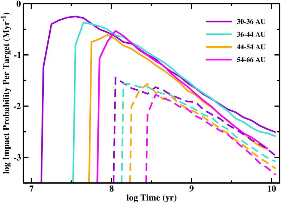
Figure 1: Probability of giant impacts in protoplanetary disks with $\Sigma=\Sigma_{0}x_{m}a^{-1}$. Solid curves: $x_{m}$ = 0.33. Dashed curves: $x_{m}$ = 0.10. Giant impacts require collisions between a massive target, $m_{t}\gtrsim 10^{25}$ g, and a projectile with $m_{p}\gtrsim 0.3m_{t}$. Colored curves illustrate the time evolution of the impact probability per target per Myr for disk annuli with boundaries listed in the legend. Giant impacts (i) happen earlier in time closer to the star and (ii) occur earlier and more frequently in more massive disks.

Fig. 1 shows the frequency (number per target per Myr) of impacts with $b$ = 0–1 as a function of time for one set of calculations from Kenyon & Bromley (2010). The curves plot the frequency of impacts between each target with mass $M_{t}\gtrsim 10^{25}$ g and a projectile with a mass $M_{p}\gtrsim q_{p}(M_{t}+M_{p})$ where $q_{p}=0.25$. As summarized in the caption, color indicates the semimajor axis of a disk annulus, ranging from 30–36 AU (violet) to 54–66 AU (magenta). Solid (dashed) lines show results for disks with $k$ = 1 and $x_{m}$ = 0.33 (0.10).

Throughout the evolution of the solar system, giant impacts are common (see also McKinnon, 1989; Stern, 1991; Canup, 2005, 2011). Initially, all planetesimals are smaller than the target mass; the frequency of giant impacts is zero. As planetesimals grow into large protoplanets, the frequency of giant impacts increases. Because protoplanets grow faster in the inner disk than in the outer disk (Kenyon & Bromley, 2004a, b), giant impacts occur earlier in the inner disk (violet and turquoise curves) than in the outer disk (orange and magenta; see also Lissauer, 1987; Stern, 1995; Kenyon & Bromley, 2005). In each disk annulus, the giant impact frequency per target rapidly rises to a clear peak when the surface density of targets and projectiles is largest. As large objects collide and merge into larger protoplanets, the giant impact frequency declines. The rate of decline, $p_{i}\propto t^{-1}$, is the rate expected for collisional evolution in a protoplanetary disk (Kenyon & Bromley, 2002; Dominik & Decin, 2003; Wyatt, 2008).

Several factors contribute to the strong variation of $p_{i}$ with initial disk mass. In these calculations, the number of Pluto-mass objects $N_{P}$ grows with increasing disk mass, $N_{P}\propto x_{m}$ (Kenyon & Bromley, 2008, 2012). For giant impacts requiring two Pluto-mass objects, the number of possible pairs of impactors scales with the square of the disk mass. In more massive disks, the larger mass of leftover planetesimals circularizes the orbits of the largest planets more effectively. Thus, gravitational focusing factors also scale with disk mass. Combining these two factors, the impact probability grows rapidly with disk mass, $p_{i}\propto x_{m}^{k}$, with $k\approx$ 3–4.

To put these results in perspective, we define $t_{N}$ as the time to the next binary-producing giant impact on a single target. If $p_{i}$ is the probability of a giant impact and if the distribution of impact orientations is random, the probability of an impact capable of producing a binary planet is $p_{bp}\approx 0.33p_{i}$. The time $t_{N}\approx p_{bp}^{-1}$. In a massive disk at 30–36 AU, $t_{N}\approx$ 5–10 Myr at an evolution time of 50–100 Myr. Binary planets then occur often, but they may be destroyed by another giant impact 5–10 Myr later. After an evolution time of 500 Myr to 1 Gyr (1–3 Gyr), $t_{N}\approx$ 150–300 Myr (500 Myr to 1 Gyr). Thus, binary icy planets form throughout the evolution of the planetary system.

3.2 Before the Giant Impact: Long-Term Accretion

After Pluto-mass objects form, they continue to interact with material from the protoplanetary disk. Although protoplanets directly accrete some of this material, they can also capture material onto temporary or bound orbits (e.g., Ruskol, 1972). To estimate the amount of material Charon or Pluto capture in the 0.5–1 Gyr in between giant impacts, we consider a simple model. Objects from the protoplanetary disk enter the planet’s Hill sphere at a rate $\dot{M}_{H}$. This material collides with other objects from the protoplanetary disk at a rate $\dot{M}_{H}\tau_{pd}$, where $\tau_{pd}$ is the optical depth of the protoplanetary disk. Collisions produce a single large remnant and some debris. The planet captures a fraction $f_{c}$ of this material into bound orbits. Although other interactions are possible (e.g., Suetsugu et al., 2011; Pires dos Santos et al., 2012; Suetsugu & Ohtsuki, 2013), this approach yields a reasonable initial estimate for captured material (e.g., Ruskol, 1972; Weidenschilling, 2002; Estrada & Mosqueira, 2006).

To derive the capture rate $\dot{M}_{c}$, we make several plausible assumptions. The optical depth of the protoplanetary disk is $\tau_{pd}\approx 3\Sigma_{pd}/4\rho_{pd}R_{pd}$, where $\Sigma_{pd}$ is the surface density and ($R_{pd}$, $\rho_{pd}$) are the radius and mass density of a typical object. During the late stages of planet formation, $R_{pd}\approx$ 100 km (Kenyon & Bromley, 2012). For simplicity, we set $\rho_{pd}$ = 1 g cm^-3. The protoplanetary disk has vertical scale height $H_{z}>R_{H}$ and surface density $\Sigma_{pd}=d_{pd}\Sigma_{0}x_{m}(a/{\rm 1~{}AU})^{-k}$ (see eq. [1]), where $\Sigma_{0}$ = 30 g cm^-2, $x_{m}$ = 1, $k$ = 1, and $d_{pd}<1$ is a depletion factor which measures the fraction of disk material lost to collisional grinding (e.g., Kenyon et al., 2008) and dynamical interactions (e.g., Morbidelli et al., 2008). For epochs when giant impacts are common, $d_{pd}\approx$ 0.1. Within the Hill sphere, collisions at $a\gtrsim\gamma R_{H}$ (with $\gamma\approx$ 0.3–0.4) produce no bound material (e.g., Toth, 1999; Martin & Lubow, 2011). For collisions at smaller $a$, $f_{c}\approx$ 0.001 (e.g., Ruskol, 1972; Weidenschilling, 2002).

With these assumptions, disk objects enter the Hill sphere of the planet at a rate $\dot{M}_{H}\approx 3\pi\Sigma_{pd}\Omega_{pd}(\gamma R_{H})^{2}$, where $\Omega_{pd}$ is the angular velocity of the planet around the Sun and the factor of three accounts for a small degree of gravitational focusing. The capture rate is then $\dot{M}_{c}\approx f_{c}\dot{M}_{H}\tau_{pd}$:

$$\dot{M_{c}}\approx 3\times 10^{10}\left({d_{pd}\over 10^{-1}}\right)^{2}\left({f_{c}\over 10^{-3}}\right)\left({\gamma_{c}\over 0.333}\right)^{2}\left({\Sigma_{0}\over{\rm 30~{}g~{}cm^{-2}}}\right)^{2}\left({R\over R_{P}}\right)^{2}\left({R_{pd}\over{\rm 100~{}km}}\right)^{-1}\left({a\over{\rm 20~{}AU}}\right)^{-3/2}~{}{\rm g~{}yr^{-1}}.$$ (2)

After $\sim$ 0.1–1 Gyr, modest reservoirs of material orbit Charon–Pluto mass planets. Pluto captures 3–30 $\times 10^{18}$ g of orbiting debris. With a smaller radius and gravity, Charon attracts 1–10 $\times 10^{18}$ g.

To estimate the collision frequency of captured material, we assume each fragment has radius $R_{f}\sim$ 1 km, mass $M_{f}\sim 4\times 10^{15}$ g, orbital semimajor axis $a_{f}\sim$ 1000 $R_{P}$ ($\sim 0.25R_{H}$), eccentricity $e_{f}\sim 0.1$, and inclination $i_{f}\sim\pi/20$. With $10^{3}-10^{4}$ fragments on randomly oriented orbits, the collision rate is $n_{f}\sigma_{f}v_{f}\approx$ 1–10 $(R_{f}/{\rm 1~{}km})^{-1}$ Gyr^-1, where $n_{f}$ is the number density, $\sigma_{f}$ is the cross-section, and $v_{f}$ is the relative velocity. In a cloud of 1 km objects, collisions are rare. Smaller fragments collide more frequently.

To constrain the total specific angular momentum $L$ of the cloud, we set the specific angular momentum per fragment $L_{f}\approx(GM_{P}a_{f}(1-e_{f}^{2}))^{1/2}$. If each vector $\bf L_{f}$ is randomly oriented, the cloud has a typical $\bf L\approx$ 0 with a standard deviation of roughly $\sqrt{N}L_{f}$. Thus, there is a reasonable probability that a cloud of fragments has a net prograde or retrograde rotation around Pluto.

Prior to impact, a low mass cloud of fragments probably surrounds Pluto. This mass depends on the typical particle size and the depletion of the protoplanetary disk. If collisions within Pluto’s Hill sphere yield large fragments with $R_{f}\gtrsim$ 1 km, the fragments occupy a large volume, rarely collide, and have a small net prograde or retrograde angular momentum. Despite a potentially significant mass, this material makes little or no contribution to the formation of low mass satellites.

If collisions within Pluto’s Hill sphere yield very small fragments, they collide more frequently and may produce a collisional cascade. This process slowly reduces the circumplanetary mass. With a small net prograde or retrograde $\bf L$, collisions may produce a disk of material with $a\ll a_{f}$ (e.g., Brahic, 1976, 1977). Although the properties of this disk are uncertain, debris from the Pluto–Charon impact may interact with pre-existing disk material. Captured material may then contribute to the formation of low mass satellites.

For New Horizons, captured material at large $a$ is challenging to detect and an unlikely hazard. Although 1 km fragments are detectable, they have small filling factor and are not worth a detailed search. Within Pluto–Charon’s Hill sphere, the total collision probability between a captured fragment and New Horizons is $\lesssim 10^{-13}$ throughout the flyby.

3.3 After the Giant Impact: Dynamical Spreading of the Circumbinary Ring

Shortly after the formation of the Pluto–Charon binary, icy material with a total mass of $\lesssim 10^{23}$ g lies at distances of 1–30 $R_{P}$ (Canup, 2011). As the evolution proceeds, most of this material resides in a ring just outside the binary system. To understand whether a circumbinary ring of debris might expand into a disk, we evaluate time scales for interactions among the ensemble of debris particles and between the binary and the debris. Particles of debris initially orbit with $a\approx$ 1–30 $R_{P}$ (Canup, 2011). The particles have radius $R$, mass density $\rho$ = 1 ${\rm g~{}cm^{-3}}$, and total mass $M_{d}$. SPH simulations of the Pluto–Charon impact suggest $R\lesssim$ 10 km and $M_{d}\approx 10^{21}-10^{23}$ g (Canup, 2011). From more general simulations of impacts, the debris probably has a range of sizes from $\lesssim$ 0.1 km up to 10 km (e.g., Leinhardt & Stewart, 2012).

Immediately after impact, collisions among debris particles produce a collisional cascade which tends to circularize particle orbits, decrease particle radii, and remove mass from the system. Although the details of this process are uncertain, it probably leads to a ring of material with surface density $\Sigma$ at $a\approx 20~{}R_{P}$. The Pluto–Charon binary then has semimajor axis $a_{PC}$ = 5–10 $R_{P}$, orbital period $T_{PC}$ = 1–3 d, and eccentricity $e_{PC}$ $\approx$ 0.1–0.8.

After the ring forms, two opposing mechanisms – tides from the binary and collisional damping among ring particles – drive the evolution. Tidal forces set the inner edge of the ring (e.g., Pringle, 1991; Holman & Wiegert, 1999) and impose a forced eccentricity, $e_{f}\approx 1.1(a_{PC}/a)e_{PC}$, on ring particles (e.g., Heppenheimer, 1974; Murray & Dermott, 1999; Wyatt et al., 1999; Moriwaki & Nakagawa, 2004; Lee & Peale, 2006; Tsukamoto & Makino, 2007). Angular momentum transfer from the binary to the ring leads to a maximum eccentricity, $e_{m}\approx 2e_{f}$ (e.g., Wyatt et al., 1999; Moriwaki & Nakagawa, 2004) The time scale for secular perturbations from tides to raise $e$ is

$$t_{s}\approx 300\left({a\over 20R_{P}}\right)^{7/2}\left(1+{3\over 2}e_{PC}^{2}\right)^{-1}T_{PC}$$ (3)

Aside from $a$, this time scale is independent of the properties of the ring. For $T_{PC}$ = 1 d, $t_{s}\approx$ 1 yr.

Physical collisions transfer angular momentum among ring particles (Goldreich & Tremaine, 1978; Hornung et al., 1985), which tends to circularize their orbits (e.g., Lynden-Bell & Pringle, 1974; Goldreich & Tremaine, 1978). If $\Omega$ is the angular velocity of ring particles with number density $n$, cross-section $\sigma$, and relative velocity $v$, the time scale for physical collisions is $t_{c}\approx(dn/dt)^{-1}\approx(n\sigma v)^{-1}\approx\rho R/\Sigma\Omega$. Thus,

$$t_{c}\approx 450\left({R\over{\rm 1~{}km}}\right)\left({a\over 20~{}R_{P}}\right)^{7/2}\left({10^{22}~{}{\rm g}\over M_{d}}\right)T_{PC}~{}.$$ (4)

In an optically thick ring with $M_{d}/Ra^{2}\gtrsim$ 1.5, the collision time is similar to or shorter than the secular time.

When collisions are frequent, angular momentum transfer among ring particles slows the precession, prevents high velocity collisions, and lessens the impact of destructive collisions. To conserve the angular momentum absorbed from the central binary, the ring must expand to larger $a$ (Lin & Papaloizou, 1979a, b). Tides input angular momentum into the ring at a rate $\dot{L}\approx fq_{PC}^{2}a_{PC}^{2}\Omega_{PC}^{2}$, where $f$ is a constant of order unity (Lin & Papaloizou, 1986a). Setting the rate of angular momentum input equal to $\dot{L}=\dot{a}\Omega a/2$, the expansion rate $\dot{a}$ for the ring is

$$\dot{a}\approx 5~{}f~{}\left({a\over 20R_{P}}\right)^{-1/2}R_{P}~{}{\rm yr^{-1}}~{}.$$ (5)

The ring spreads from 20 $R_{P}$ to 60 $R_{P}$ in 5–10 yr, $\sim$ 20–40 collision times.

Although understanding the early evolution of the ring requires a detailed analytic (e.g., Rafikov, 2013) or numerical (e.g., Scholl et al., 2007; Paardekooper et al., 2012) calculation, these estimates suggest a narrow ring of material plausibly expands into a disk at least as fast as satellites grow from the debris (eq. [4]; see §3.4 below). For the very large collision velocities of particles with eccentricity $e_{m}$, destructive collisions can reduce typical particle sizes from $\sim$ 1 km to 0.1 km over 20–40 collision times. Significant mass removal on this time scale also seems likely.

3.4 Growth of Satellites in the Particle Disk

As the circumbinary ring of small particles expands, collisional damping reduces particle random velocities. When random velocities are low enough, collisions produce merged objects instead of a cloud of fragments. Dynamical friction lowers the random velocities of the largest objects, promoting additional growth. Eventually satellites reach sizes of 1–10 km, when they may begin to migrate through the disk.

To perform numerical calculations of planet and satellite formation, we use Orchestra, an ensemble of computer codes for the formation and evolution of planetary systems. Currently, Orchestra consists of a radial diffusion code which computes the time evolution of a gaseous or particulate disk (Bromley & Kenyon, 2011a), a multiannulus coagulation code which computes the time evolution of a swarm of planetesimals (Kenyon & Bromley, 2004a, 2008), and an $n$-body code which computes the orbits of gravitationally interacting protoplanets (Bromley & Kenyon, 2006, 2011a, 2013). The coagulation code uses statistical algorithms to evolve the mass and velocity distributions of low mass objects with time; the $n$-body algorithm follows the individual trajectories of massive objects. Within the coagulation code, Orchestra includes algorithms for treating interactions between coagulation mass bins and the $n$-bodies (Bromley & Kenyon, 2006). To treat interactions between small particles and the $n$-bodies more rigorously, the $n$-body calculations include tracer particles. Massless tracer particles allow us to calculate the evolution of the orbits of small particles in response to the motions of massive protoplanets. Massive tracer particles enable calculations of the response of $n$-bodies to the changing gravitational potential of small particles (Bromley & Kenyon, 2011a, b, 2013).

We perform calculations on a cylindrical grid with inner radius $a_{in}$ and outer radius $a_{out}$. The model grid contains $K$ concentric annuli with widths $\delta a_{i}=0.035a_{i}$ centered at semimajor axes $a_{i}$. Calculations begin with a cumulative mass distribution $N_{c}(m_{ik})\propto m_{ik}^{-q^{\prime}}$ of particles with mass density $\rho$ = 1 g cm^-3 and maximum initial mass $m_{0}$. For comparison with investigators that quote differential size distributions with $N\propto m^{-q}$, $q^{\prime}$ = $q$ + 1. Here, we adopt an initial $q^{\prime}_{0}$ = 0.17; thus most of the initial mass is in the largest objects.

Planetesimals have horizontal and vertical velocities $h_{ik}(t)$ and $v_{ik}(t)$ relative to a circular orbit. The horizontal velocity is related to the orbital eccentricity, $e_{ik}^{2}(t)$ = 1.6 $(h_{ik}(t)/V_{K,i})^{2}$, where $V_{K,i}$ is the circular orbital velocity in annulus $i$. The orbital inclination depends on the vertical velocity, $sin^{2}i_{ik}(t)$ = $(2(v_{ik}(t)/V_{K,i})^{2})$.

The mass and velocity distributions of the planetesimals evolve in time due to inelastic collisions, drag forces, and gravitational encounters. As summarized in Kenyon & Bromley (2004a, 2008), we solve a coupled set of coagulation equations which treats the outcomes of mutual collisions between all particles with mass $m_{j}$ in annuli $a_{i}$. We adopt the particle-in-a-box algorithm, where the physical collision rate is $n\sigma vf_{g}$, $n$ is the number density of objects, $\sigma$ is the geometric cross-section, $v$ is the relative velocity, and $f_{g}$ is the gravitational focusing factor. Depending on physical conditions in the disk, we derive $f_{g}$ in the dispersion or the shear regime (Kenyon & Bromley, 2012). For a specific mass bin, the solutions include terms for (i) loss of mass from mergers with other objects and (ii) gain of mass from collisional debris and mergers of smaller objects.

Collision outcomes depend on the ratio $Q_{c}/Q_{D}^{*}$, where $Q_{D}^{*}$ is the collision energy needed to eject half the mass of a pair of colliding planetesimals to infinity and $Q_{c}$ is the center of mass collision energy. From detailed $n$-body and smooth particle hydrodynamics calculations (Benz & Asphaug, 1999; Leinhardt et al., 2008; Leinhardt & Stewart, 2009),

$$Q_{D}^{*}=Q_{b}R^{\beta_{b}}+Q_{g}\rho R^{\beta_{g}}$$ (6)

where $Q_{b}R^{\beta_{b}}$ is the bulk component of the binding energy, $Q_{g}\rho R^{\beta_{g}}$ is the gravity component of the binding energy, and $R$ is the radius of a planetesimal. We adopt $Q_{b}$ = $2\times 10^{5}$ erg g^-1 cm^0.4, $\beta_{b}=-0.40$, $Q_{g}$ = 0.22 erg g^-2 cm^1.7, and $\beta_{g}$ = 1.30 (Leinhardt et al., 2008; Leinhardt & Stewart, 2009).

For two colliding planetesimals with masses $m_{1}$ and $m_{2}$, the mass of the merged planetesimal is

$$m=m_{1}+m_{2}-m_{ej}~{},$$ (7)

where the mass of debris ejected in a collision is

$$m_{ej}=0.5~{}(m_{1}+m_{2})\left(\frac{Q_{c}}{Q_{D}^{*}}\right)^{9/8}~{}.$$ (8)

To place the debris in our grid of mass bins, we set the mass of the largest collision fragment as $m_{L}=0.2m_{esc}$ and adopt a cumulative mass distribution $N_{c}\propto m^{-q_{d}}$ with $q_{d}$ = 0.833, roughly the value expected for a system in collisional equilibrium (Dohnanyi, 1969; Williams & Wetherill, 1994; Tanaka & Ida, 1996; O’Brien & Greenberg, 2003; Kobayashi & Tanaka, 2010). This approach allows us to derive ejected masses for catastrophic collisions with $Q_{c}\sim Q_{D}^{*}$ and for cratering collisions with $Q_{c}\ll Q_{D}^{*}$ (see also Wetherill & Stewart, 1993; Williams & Wetherill, 1994; Tanaka & Ida, 1996; Stern & Colwell, 1997; Kenyon & Luu, 1999; O’Brien & Greenberg, 2003; Kobayashi & Tanaka, 2010).

To compute the evolution of the velocity distribution, we include collisional damping from inelastic collisions and gravitational interactions. For inelastic and elastic collisions, we follow the statistical, Fokker-Planck approaches of Ohtsuki (1992) and Ohtsuki et al. (2002), which treat pairwise interactions (e.g., dynamical friction and viscous stirring) between all objects in all annuli. As in Kenyon & Bromley (2001), we add terms to treat the probability that objects in annulus $i_{k}$ interact with objects in annulus $i_{l}$ where $k,l$ = 1–$K$ (Kenyon & Bromley, 2004a, 2008). We also compute long-range stirring from distant oligarchs (Weidenschilling, 1989).

In the $n$-body code, we directly integrate the orbits of objects with masses larger than a pre-set ‘promotion mass’ $m_{pro}$. The calculations allow for mergers among the $n$-bodies. Additional algorithms treat mass accretion from the coagulation grid and mutual gravitational stirring of $n$-bodies and mass batches in the coagulation grid. To treat interactions among proto-satellites, we set $m_{pro}=10^{17}-10^{19}$ g.

Our calculations follow the time evolution of the mass and velocity distributions of objects with a range of radii, $r_{ij}=r_{min}$ to $r_{ij}=r_{max}$. To track the amount of material ejected by radiation pressure, we set $r_{min}$ = 20 $\rm\mu{\rm m}$. The upper limit $r_{max}$ is always larger than the largest object in each annulus.

For this initial exploration of satellite growth in a circumbinary ring, we derive results for (i) pure coagulation calculations with fragmentation and no $n$-body component and (ii) hybrid calculations with the $n$-body component but no fragmentation. Aside from enabling a broader set of calculations per unit cpu time, these two sets of calculations probably bracket the likely time scales for satellite growth around the Pluto–Charon binary. With no stirring from the central binary, the pure coagulation calculations set a firm lower limit on the growth time. With no collisional damping or dynamical friction from small objects and no stirring from the central binary, hybrid calculations without fragmentation likely establish an upper limit on the growth time. Together, the two sets of calculations show that the likely growth time is comparable to or longer than the time for the ring to spead (§3.3).

We perform both sets of calculations on a grid of 32 concentric annuli extending from $a_{in}$ = 15 $R_{P}$ to $a_{out}$ = 50 $R_{P}$. This cylindrical grid provides a reasonably accurate representation of plausible orbits of debris particles from the giant impact around a circular binary system with an initial separation of 5 $R_{P}$ (Canup, 2011). The inner edge of this grid lies roughly at the innermost stable orbit around a newly-formed Pluto–Charon binary. The outer edge allows the grid to cover a radial extent roughly two times larger than the current radial extent (39–57 $R_{P}$) of the satellite system. For a ring of fixed mass $M_{d}$ and aspect ratio $a_{out}/a_{in}\approx 3.33$, we expect satellites to form at roughly the same relative positions with roughly the same mass on a formation time which scales as $a_{in}^{2.5}$. Thus, choosing $a_{in}$ = 30 $R_{P}$ and $a_{out}$ = 100 $R_{P}$ results in formation times that are roughly 5.5 times longer than those described below.

3.4.1 Pure Coagulation Calculations

These calculations begin with a ring of material surrounding a single central object with mass equivalent to the Pluto–Charon binary. The total mass in the ring ranges between $M_{d}=3\times 10^{19}$ g and $M_{d}=3\times 10^{21}$ g, with an initial surface density distribution $\Sigma\propto a^{-1}$. Within each annulus of the ring, the solid particles range in size from 20 $\rm\mu{\rm m}$ to 0.1 km. Radiation pressure probably ejects particles with $R\lesssim$ 20 $\rm\mu{\rm m}$ on short time scales (e.g., Burns et al., 1979; Poppe & Horányi, 2011). Although particles with $R\gtrsim$ 0.1 km might lie within the ring, adopting a maximum particle size of 0.1 km provides a rough upper limit on the amount of mass lost to a collisional cascade. We consider calculations starting with several 1 km objects in the next section. To allow the system to find an equilibrium between the large orbital eccentricity expected of material ejected from the central binary and the small eccentricity expected from collisional damping, we adopt an initial eccentricity $e_{0}$ = 0.1 and an initial inclination $i_{0}/e_{0}$ = 0.5.

All calculations follow a similar pattern. With the large initial $(e,i)$ of all particles, collisions among large particles are destructive and produce copious amounts of smaller particles. Among the smaller particles, collisional damping is effective. Through dynamical friction, smaller particles damp the orbits of the larger particles. Thus, the $(e,i)$ for all particles declines with time. Collisions become less destructive. Eventually, collisional velocities become small enough to promote growth over destruction. During this phase, roughly 25% of the initial mass is ground down into particles smaller than 20 $\rm\mu{\rm m}$. Radiation pressure ejects this material from the binary (e.g., Burns et al., 1979; Kennedy & Wyatt, 2011).

After the system reaches a low velocity equilibrium, the largest particles begin to grow rapidly. During a very short phase of runaway growth, objects grow from roughly 0.1 km to 3–30 km. As the largest objects grow, they gravitationally stir the smaller particles. Once the largest objects contain most of the mass, stirring dominates collisional damping. The orbital $(e,i)$ of the smaller objects rapidly increases, reducing gravitational focusing factors and halting runaway growth. At the end of runaway growth, each annulus contains a handful of proto-satellites with radii of 3–30 km.

Following runaway growth, the evolution of the system stalls. The proto-satellites rapidly accrete any small particles left in their annuli. Because the small particles contain so little mass, this growth of the large particles is very small. In the particle-in-a-box approximation adopted for these pure coagulation calculations, the probability of collisions among large objects is small. Thus, the sizes of the proto-satellites reach a rough steady state set approximately by the initial mass in each annulus of the grid.

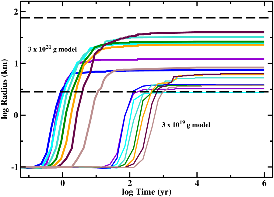
Figure 2: Radius evolution for satellites in a disk surrounding the Pluto–Charon binary. The dashed lines indicate the lower limit for the radius of Styx ($A$ = 1) and the upper limit for the radius of Hydra ($A$ = 0.04) assuming a mass density $\rho$ = 1 g cm^-3. The thin (thick) lines plot results for a model with an initial disk mass of $M_{d}=3\times 10^{19}$ g ($M_{d}=3\times 10^{21}$ g) in solid objects with initial radii of 0.1 km and smaller. Each line indicates the radius evolution for the largest object in annuli at 17.5 $R_{P}$ (violet), 20 $R_{P}$ (blue), 23 $R_{P}$ (cyan), 26.5 $R_{P}$ (turquoise), 30.5 $R_{P}$ (green), 35 $R_{P}$ (orange), 40.5 $R_{P}$ (maroon), and 46.5 $R_{P}$ (brown). Satellites grow faster in more massive disks. The range of model radii span the range inferred for satellites of Pluto–Charon.

Figure 2 illustrates the growth of satellites for calculations with $M_{d}=3\times 10^{19}$ g (thin lines) and $M_{d}=3\times 10^{21}$ g (thick lines). As summarized in the caption, each line represents the evolution in the radius of the largest object in annuli ranging in distance from 15 $R_{P}$ to 50 $R_{P}$ from the center-of-mass. In these disks, satellite growth is very rapid. After an initial period of destructive collisions, it takes only 1–100 yr for an ensemble of 0.1 km fragments to grow into 10 km satellites. The growth time is inversely proportional to the initial disk mass, $t_{g}\approx 100~{}(3\times 10^{20}~{}{\rm g}/M_{d})~{}{\rm yr}$. Once satellites reach a maximum radius of 5–50 km, growth stalls. Satellites remain at a roughly constant radius for thousands of years.

These calculations demonstrate the inevitable growth of 5–30 km satellites from an ensemble of much smaller objects. Independent of the initial orbital eccentricity, collisional damping reduces the internal velocity dispersion to levels that promote mergers during collisions. Although the collisional cascade removes roughly 25% of the initial mass, small objects grow rapidly into satellites with radii of 5–30 km.

Despite the efficiency of small satellite formation, coagulation calculations produce too many satellites. In these models, each of the 32 annuli in the calculation yields 0–3 satellites with radii of 5–30 km. Even with small number statistics, this result is much larger than the current number of known satellites. However, the coagulation calculations do not allow large-scale dynamical interactions among satellites. For the models shown in Fig. 2, satellites in adjacent annuli have orbital separations of 5–15 $R_{P}$. Thus, satellites are close enough to perturb the orbits of their nearest neighbors, leading to chaotic interactions as in simulations of terrestrial planet formation (Chambers, 2001; Kokubo & Ida, 2002; Kominami & Ida, 2004; Kenyon & Bromley, 2006).

3.4.2 Hybrid Calculations

To investigate dynamical interactions among newly-formed satellites, we now consider a suite of hybrid simulations with Orchestra. Objects in the coagulation code which reach a preset mass, $m_{pro}$, are promoted into the $n$-body code. When a satellite with $(m_{ij},e_{ij},i_{ij})$ in an annulus with semimajor axis $a_{i}$ is promoted, we assign $(e_{n},i_{n})$ = $(e_{ij},i_{ij})$, $a_{n}$ = $a_{i}+g\Delta a_{i}$, and a random orbital phase, where $g$ is a random number in the range $-0.5$ to $+0.5$. The $n$-body code converts these orbital elements into an initial $(x,y,z)$ position and an initial $(v_{x},v_{y},v_{z})$ velocity vector. The $n$-body code follows the trajectories of all promoted satellites. Algorithms within Orchestra allow $n$-bodies to interact with coagulation particles (Bromley & Kenyon, 2006, 2011a).

The starting conditions for these calculations are identical to those for the pure coagulation models. We consider three cases for the initial disk mass, $m_{d}=3\times 10^{19}$ g (low mass disk), $m_{d}=3\times 10^{20}$ g (intermediate mass disk), and $m_{d}=3\times 10^{21}$ g (massive disk). For each case, we adopt a different promotion mass: $m_{pro}=3\times 10^{17}$ g (low mass), $m_{pro}=10^{18}$ g (intermediate mass), and $m_{pro}=3\times 10^{18}$ g (high mass). These promotion masses are a compromise between the ‘optimal’ promotion mass, $m_{pro}=3-30\times 10^{16}$ g, required to allow newly formed $n$-bodies to adjust their positions and velocities to existing $n$-bodies and the practical limits required to complete calculations in a reasonable amount of time. For each combination of disk mass and promotion mass, we ran 20–25 simulations.

To check the accuracy of our results for the intermediate and high mass disks, we ran an additional 12 simulations for each of two cases with promotion masses a factor of three larger and a factor of three smaller than the promotion masses listed above. When the promotion mass is a factor of three larger, the chaotic growth phase begins later and lasts longer. Often, chaotic growth in the outer disk is well-separated in time from chaotic growth in the inner disk. This unphysical behavior contrasts with calculations with smaller promotion masses, where the timing of chaotic growth changes smoothly from the inner disk to the outer disk. As a result, these calculations have less scattering and radial mixing among proto-satellites. When the promotion mass is a factor of three smaller, the onset, character, and duration of chaotic growth changes very little. In all cases, the final number of satellites is fairly independent of promotion mass.

Because fragmentation has a small impact on the results of pure coagulation calculations per unit cpu time, these hybrid calculations do not include fragmentation. Neglecting fragmentation increases the mass available for satellite growth by roughly 25%. Without fragmentation, collisions fail to produce copious amounts of 1 m to 100 m particles. Collisional damping among these debris particles and dynamical friction between the debris and larger survivors reduces the orbital $e$ and $i$, aiding runaway growth. Thus, these hybrid calculations artificially increase the evolution time required for satellites to reach $R\gtrsim$ 10 km.

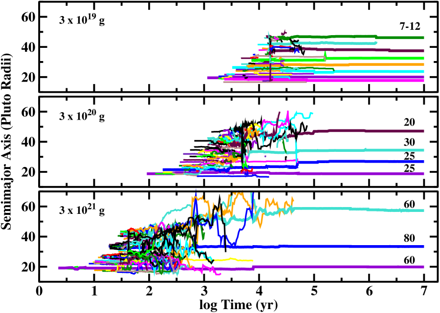
Figure 3: Semimajor axis evolution for satellites in a disk surrounding Pluto–Charon. The upper left corner of each panel lists the initial disk mass. Along the right edge of each panel, numbers indicate the radii (in km) of each satellite. More massive disks produce fewer, larger satellites than less massive disks.

Fig. 3 shows the evolution of the semimajor axes for promoted satellites orbiting a single central object with the mass of the Pluto–Charon binary. All objects begin with $r\lesssim$ 0.1 km ($m\lesssim 4\times 10^{12}$ g). The evolution time required for these objects to reach the promotion mass scales with the initial disk mass, $t_{pro}\approx 10^{3}~{}(3\times 10^{19}~{}{\rm g}/m_{d})$ yr. This time scale is roughly a factor of ten longer than derived for pure coagulation calculations with fragmentation. In the inner disk, objects have shorter orbital periods and shorter collision times. Thus, the first promoted objects appear near the inner edge of the disk. As the calculation proceeds, satellites are promoted farther and farther out in the disk. Eventually, a few promoted objects appear in the outer disk.

Every calculation experiences chaotic growth (Goldreich et al., 2004; Kenyon & Bromley, 2006). During chaotic growth, the satellites scatter one another throughout the grid. Because objects grow fastest in the most massive disks, chaotic growth begins earlier – $\sim$ 100 yr – in the high mass disk and much later – $\sim 10^{4}$ yr – in the low mass disk. Chaotic growth is also ‘stronger’ in more massive disks. In more massive disks, massive large satellites are more numerous and generate larger radial excursions of smaller satellites than in lower mass disks.

Throughout the evolution shown in Fig. 3, the $n$-bodies slowly accrete the very small planetesimals remaining in the coagulation grid. The number of leftovers correlates well with the number of $n$-bodies. Thus, the total mass in leftover planetesimals within the coagulation grid approaches zero as the number of $n$-bodies reaches a minimum.

In all of these calculations, the final number of satellites correlates inversely with the initial disk mass. In massive disks with $M_{d}=3\times 10^{21}$ g, there are usually 2 or 3 massive satellites with $r\approx$ 50–80 km at the end of the calculation. As we reduce the initial disk mass, the calculations produce more satellites with smaller masses. In intermediate mass disks with $M_{d}=3\times 10^{20}$ km, chaotic growth leaves all of the initial mass in 4–5 satellites with radii of 20–30 km. In low mass disks, there are very few mergers during chaotic growth. After $\sim 10^{7}$ yr, there are typically 7–9 satellites with radii of 7–12 km.

To test how outcomes change with the initial size distribution, we consider a suite of 15 simulations with two additional 10 km planetesimals placed randomly in the grid. These large planetesimals stir their surroundings and thus counteract collisional damping by nearby small planetesimals. With much larger masses than any other planetesimals in the grid, they have large collisional cross-sections and can grow very rapidly.

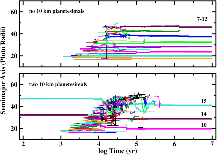
Figure 4: As in Fig. 3 for an initial disk mass $m_{d}\approx 3\times 10^{19}$ g composed of 0.1 km and smaller planetesimals. Upper panel: evolution without larger planetesimals; lower panel: evolution with two 10 km planetesimals. Calculations with a several initial large planetesimals yield fewer, larger satellites than calculations without large planetesimals.

Fig. 4 compares the time evolution of the semimajor axes for $n$-bodies in calculations with (lower panel) and without (upper panel) two additional massive planetesimals. In standard calculations with $M_{d}=3\times 10^{19}$ g, there is a short period of chaotic growth at $\sim 10^{4}-10^{5}$ yr followed by a long quiescent period with an occasional merger. When there are two large planetesimals at the onset of the calculation, these planetesimals slowly accumulate small planetesimals. Meanwhile, small planetesimals in the rest of the disk rapidly grow to sizes (4–5 km) that allow promotion into the $n$-body code. From Fig. 4, the time scale for these objects to reach the promotion mass is roughly $10^{3}-10^{4}$ yr independent of the two large satellites. However, stirring by the two large satellites promotes an earlier oligarchic growth phase which enables more uniform growth of the largest planetesimals. Thus, there are many more promoted objects and a more intense chaotic growth phase. In addition to the two initial massive planetesimals, one or two other planetesimals accrete all of the other promoted objects. After $\sim 10^{5}$ yr, there are only a few small $n$-bodies left. The 3–4 massive satellites accrete these objects in a few hundred thousand years.

This result is typical of all calculations in low or intermediate mass disks that begin with a few large (10 km) planetesimals placed randomly throughout the grid. Stirring by the large objects slows runaway growth and allows a larger group of oligarchs to grow rapidly. Although these oligarchs reach the promotion mass on similar time scales, many more of them reach the promotion mass. Typically, calculations with initial large planetesimals produce 2–4 times as many $n$-bodies as calculations without large planetesimals. Stirring by the 10 km planetesimals and interactions among the many $n$-bodies leads to a very active phase of chaotic growth. During chaotic growth, the radial excursions of the $n$-bodies are 2–3 times larger in semimajor axis. Collisions among $n$-bodies are more frequent, leading to a system with fewer, but more massive, satellites. With a set of two initially large planetesimals, low (intermediate) mass disks produce 3–4 (2–3) massive satellites instead of 7–9 (4–5).

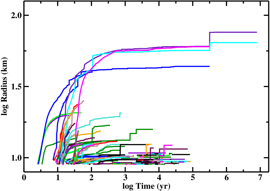
Figure 5: Radius evolution for $n$-bodies. The calculation begins with $m_{d}=3\times 10^{21}$ g and $m_{pro}=3\times 10^{18}$ g. Once a few large objects form, they gradually accrete all of the smaller $n$-bodies.

For all of these hybrid calculations, the radius evolution follows a standard pattern (Fig. 5). As in Fig. 2, the largest objects in the coagulation grid grow from 0.1 km to 1–10 km. Once they are promoted into the $n$-body grid, they interact with objects in the coagulation grid and all of the promoted objects in the $n$-body grid. Unlike the pure coagulation calculations, growth does not stall at 5–30 km. The extra interactions between promoted objects and the larger volume sampled by scattered objects enables a few large objects to accumulate nearly all of the remaining mass in the grid. Thus, these objects reach radii that are 30% to 100% larger (and 2–8 times more massive) than the largest objects in the pure coagulation calculations.

3.4.3 Summary of Coagulation and Hybrid Calculations

The suite of pure coagulation and hybrid calculations demonstrates that the Pluto–Charon satellites grow rapidly from a disk of small planetesimals. In calculations with fragmentation, destructive collisions grind down roughly 25% of the initial disk mass into 20 $\mu$m particles which are ejected from the binary system. Collisional damping among larger debris particles reduces orbital eccentricity of 0.1–10 m objects. Dynamical friction between these small planetesimals and the surviving large planetesimals damps the orbital eccentricities of the largest objects, greatly reducing the frequency of destructive collisions and enabling rapid growth of surviving planetesimals. Thus, fragmentation removes mass and aids the eventual rapid growth of satellites.

In hybrid calculations without fragmentation, less collisional damping and dynamical friction slow growth considerably. However, satellites still grow on time scales similar to the expansion time for the central binary. The number of satellites $N_{s}$, typical satellite radius $R_{s}$, and the time for satellites to reach their final mass $t_{f}$ scales with the initial mass of the planetesimal disk. For calculations without any large (10 km) fragments at $t=0$ and $M_{d}\approx 3-300\times 10^{19}$ g, we infer

$$\left.\begin{array}[]{l}N_{s}\\ \\ R_{s}\\ \\ t_{f}\\ \end{array}\right\}=\left\{\begin{array}[]{ll}2^{22.5-{\rm log}~{}M_{d}}\\ \\ 27.5\left({3\times 10^{20}~{}{\rm g}\over M_{d}}\right)^{0.425}~{}{\rm km}&~{}~{}~{}~{}~{}~{}~{}~{}~{}~{}~{}~{}~{}{\rm no~{}initial~{}large~{}fragments}\\ \\ 10^{4}\left({3\times 10^{20}~{}{\rm g}\over M_{d}}\right)~{}{\rm yr}\end{array}\right.$$ (9)

In low and intermediate mass disks, calculations with several 10 km fragments produce fewer satellites with larger masses. For $M_{d}\approx 3-30\times 10^{19}$ g, $N_{s}\approx$ 3–5 and $R_{s}\approx$ 15–60 km instead of the $N_{s}\approx$ 4–10 and $R_{s}\approx$ 7–30 km for calculations without large fragments. Because large fragments tend to sweep up any small planetesimals, calculations with fragments yield a smaller spread in the number and masses of planetesimals than calculations without fragments.

3.4.4 Observations: Comparisons and Predictions

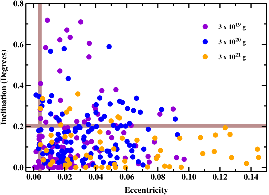
Figure 6: Distribution of orbital eccentricity $e$ and inclination $i$ for satellites produced in disks with initial masses of $3\times 10^{19}$ g (violet points), $3\times 10^{20}$ g (blue points), and $3\times 10^{21}$ g (orange points). Although there is no clear correlation of average orbital inclination with disk mass, disks with larger initial masses produce satellites with larger average $e$. The horizontal and vertical bars indicate the average of the measured eccentricity and inclination for Nix ($e_{N}$ and $i_{N}$) and Hydra ($e_{H}$ and $i_{H}$) from the 2007 Jacobson PLU017 JPL satellite ephemeris. For the model satellites, 10% have $e\lesssim e_{H,N}$ and 83% have $i\lesssim i_{H,N}$.

To conclude this section, Fig. 6 plots pairs of $(e,i)$ for satellites that survive for $10^{7}$ yr. For most satellites, the orbital inclination is small: the average inclination is $<i>$ = 0.1^∘ $\pm$ 0.2^∘. Despite the apparent excess of high $i$ objects at small $e$ for the low and intermediate mass disks, the average $i$ and the dispersion in the average do not vary with initial disk mass. The average $e$ grows with disk mass, however, with $<e>=0.02\pm 0.02$ for $M_{d}=3\times 10^{19}$ g, $<e>=0.03\pm 0.02$ for $M_{d}=3\times 10^{20}$ g, and $<e>=0.06\pm 0.06$ for $M_{d}=3\times 10^{21}$ g. For small and intermediate initial disk masses, the average eccentricity is very low. For large disk masses, the $<e>$ is a factor of 2–3 larger.

Although the final orbital elements of satellites are independent of the promotion mass, $e$ depends on the initial masses of the largest planetesimals. When we add several large planetesimals to the initial distribution of 0.1 km and smaller planetesimals, the calculations yield fewer satellites with larger masses (Fig. 4). As in calculations with larger total disk masses, a few large satellites stir up their surroundings more than many smaller satellites. These satellites then have larger $e$.

The orbital elements of model satellites agree reasonably well with the observed elements of the Pluto–Charon satellites. Roughly 10% of the model satellites have $e\lesssim e_{H}$, where $e_{H}$ is the orbital eccentricity of Hydra. Nearly all (83%) satellites have orbital inclinations $i\lesssim i_{H}$, where $i_{H}$ is the inclination of Hydra. Satellites with integer period ratios are also common. For calculations with $M_{d}=3\times 10^{21}$ g, 60% of the outer satellites have period ratios reasonably close to the 5:3, 2:1, or 3:1 commensurabilities with the inner satellite. Disks with smaller initial masses produce more closely-packed, lower mass satellites which often lie close to the 3:2 and 4:3 commensurabilities. For these lower mass disks, 50% to 70% of satellites have period ratios within a few per cent of the 4:3, 3:2, 5:3, 2:1, or 3:1 commensurabilities.

These results are encouraging. Model satellites often lie close to the observed orbital commensurabilities in the Pluto–Charon satellites. The derived inclinations of model satellites also agree very well with observations. Although lower mass disks produce satellites with the smallest $e$, derived eccentricities for all calculations are factor of 4–20 larger than observed. Thus, the calculations have two successes – the small inclinations and the likelihood of close orbital commensurabilities – and one failure – the lack of very small eccentricities for the satellites.

In addition to satellite formation, pure and hybrid coagulation calculations leave behind remnant disks of small particles. When satellites are close to their final masses, remnant disk particles have large orbital eccentricities and large vertical scale heights. At this epoch, it is more likely for small disk particles to collide with one another than to collide with a 10–15 km satellite. A collisional cascade gradually depletes the remnant disk (e.g., Kenyon & Bromley, 2008, 2010, and references therein). For conditions in the Pluto–Charon system, the remnant disk mass at $\sim 10^{4}$ yr is roughly $10^{15}-10^{17}$ g and declines with time as $t^{-1}$ (see also Dominik & Decin, 2003; Kenyon & Bromley, 2004a). Thus, the disk has a fairly substantial mass for 1–10 Myr. At later times, the loss of material from collisional grinding reaches an equilibrium with material captured from collisions between small Kuiper Belt objects and the satellites (e.g. Stern et al., 2006; Poppe & Horányi, 2011). Based on current analyses of the capture rate, this equilibrium mass is roughly $10^{13}-10^{14}$ g.

If satellites have much larger radii, $\sim$ 40–70 km, they accrete small particles faster than the collisional cascade removes them. The remnant disk mass then declines more rapidly, on time scales of roughly $10^{5}$ yr instead of 1–10 Myr. Direct albedo measurements from New Horizons will test this possibility.

To explore the outcomes of formation models in more detail, we now consider numerical calculations of satellite migration through the circumbinary disk surrounding Pluto–Charon. Aside from testing analytic estimates for essential migration parameters, these calculations allow us to estimate the frequency of migration-driven mergers and to examine the evolution of $e$ and $i$ for an ensemble of migrating satellites.

3.5 Migration of Satellites Through the Circumbinary Disk

3.5.1 Background

Throughout the growth process outlined in §3.4, gravitational scattering plays an important role in the local structure of the disk. The Hill radius,

$$R_{H}\approx 10\left({R\over 1~{}{\rm km}}\right)\left({a\over{\rm 20~{}R_{P}}}\right)~{}{\rm km}~{},$$ (10)

defines the region where the gravity of a satellite overcomes the gravity of Pluto–Charon. If the satellite can clear its orbit of small objects, it can open a gap in the radial distribution of solids. For convenience, we define the Hill radius necessary for a satellite to open up a gap in a dynamically cold disk surrounding the Pluto–Charon binary (e.g., Rafikov, 2001; Bromley & Kenyon, 2013):

$$R_{gap}\approx 19\left({v_{r}\over{75~{}{\rm cm~{}s^{-1}}}}\right)^{2/3}\left({M_{d}\over 10^{20}~{}{\rm g}}\right)^{1/3}\left({R\over{\rm 1~{}km}}\right)^{-1/3}\left({a_{c}\over 20~{}R_{P}\ }\right)^{1/3}~{}{\rm km}~{}.$$ (11)

Satellites with $R_{H}$ $\approx$ 20 km have physical radii $R\approx$ 2 km (eq. [10]). For circumbinary disks with $M_{d}\approx 10^{20}$ g, satellites with $R\gtrsim$ 2 km open gaps in the disk. All four Pluto–Charon satellites have $R\gtrsim$ 3 km. Thus, each can open a gap in a cold circumbinary disk.

For satellites with $R\gtrsim R_{gap}$, there are two possible modes of migration (e.g., Bromley & Kenyon, 2011b, 2013). If the satellite can (i) clear a gap in its corotation zone and (ii) migrate across this gap in one synodic period, the satellite undergoes fast migration. Satellites with $R_{H}>R_{gap}$ ($R_{H}=R_{gap}$) satisfy the first (second) condition. Although the size of the gap grows with $R$; the synodic period decreases with $R$. Thus, there is a maximum Hill radius – defined as $R_{fast}$– which allows a satellite to satisfy the second condition. With this definition, satellites with $R_{gap}\lesssim R_{H}\lesssim R_{fast}$ undergo fast migration. For the Pluto–Charon binary,

$$R_{fast}\approx 20\left({M_{d}\over 10^{20}~{}{\rm g}}\right)^{1/2}\left({a\over 20~{}R_{P}\ }\right)^{3/2}~{}{\rm km}.$$ (12)

Depending on the disk properties and satellite location, this Hill radius corresponds to objects with physical radii of a few kilometers. Coupled with the limits on $R_{gap}$, satellites with physical radii of 2–5 km undergo fast migration. These objects drift radially inward or outward at a rate

$$\dot{a}_{fast}\approx\pm 5\left({M_{d}\over 10^{20}~{}{\rm g}}\right)\left({a\over 20R_{P}\ }\right)^{3/2}{\rm km~{}yr^{-1}}~{}.$$ (13)

On time scales comparable to the accretion time of 200 yr, 2–5 km objects drift roughly 1 $R_{P}$. Thus, growth and migration are simultaneous.

Massive satellites with $R_{H}>R_{fast}$ migrate through the disk at a rate that depends on the disk viscosity. In gaseous disks with a large viscosity, this “gap” migration can transport gas giants from 5–10 AU to within a few stellar radii of a solar-type star in $\sim$ 1 Myr (Lin & Papaloizou, 1986b; Ward, 1997; Nelson & Papaloizou, 2004). In a disk of particles, the smaller viscosity derived from gravitational scattering leads to a smaller gap migration rate (Ida et al., 2000; Cionco & Brunini, 2002; Kirsh et al., 2009; Bromley & Kenyon, 2011b; Ormel et al., 2012). For a circumbinary disk in Pluto–Charon, the expected migration rate is (Bromley & Kenyon, 2013)

$$\dot{a}_{II}\approx-0.15\left({M_{d}\over 10^{20}~{}{\rm g}}\right)\left({R\over{\rm 20~{}km}}\right)\left({a\over 20R_{P}\ }\right)^{1/2}{\rm km~{}yr^{-1}}~{}.$$ (14)

Satellites with $R\approx$ 10–20 km migrate 1 $R_{P}$ every $10^{4}$ yr. This rate is slower than the growth rate. Thus, large satellites grow faster than they migrate.

3.5.2 Migration of a Single Satellite

To explore satellite migration in a disk surrounding the Pluto–Charon binary, we use the $N$-body component of the Orchestra code. In this mode, the calculations directly track interactions between satellites and massive “super-particles” that represent small particles in the disk. For massive objects within a disk around a single central object, our calculations (Bromley & Kenyon, 2011a, b) reproduce published results of previous investigators (e.g., Malhotra, 1993; Hahn & Malhotra, 1999; Kirsh et al., 2009). Our investigation of migration within Saturn’s rings includes extensive tests with gaps in the disk, orbital resonances, and the gravitational perturbations of distant massive moons outside resonance (Bromley & Kenyon, 2013). To test the theoretical limits on migration rates in a disk surrounding Pluto–Charon, we first consider calculations of a lone satellite with $R\approx R_{gap}-R_{fast}$ within a particle disk around a single central object with the combined mass of Pluto–Charon. We then consider how a binary central object modifies the mode and rate of migration. Because the hybrid calculations often produce many small satellites, we conclude this section with simulations of multiple satellites orbiting a central binary.

For this suite of simulations, we adopt a disk surface density distribution, $\Sigma\propto a^{-1}$, with a fixed mass of $3\times 10^{20}$ g. The disk extends from $a$ = 20 $R_{P}$ to $a$ = 70 $R_{P}$ around a single object with a radius of 1 $R_{P}$ or a binary with a separation of 5 $R_{P}$. We follow an ensemble of super-particles and satellites in an annulus of full width of 5 $R_{P}$. Super-particles have masses of 1/2000^th the mass of the satellite. These objects interact with the satellite and the central mass, but not with each other. Satellites have fixed bulk mass density, $\rho=1$ g cm^-3.

At the start of each simulation, super-particles are dynamically cold. Thus, the disk is geometrically thin, with $H_{z}/R_{H}\lesssim$ 1. Particle trajectories evolve solely by interactions with the central (single or binary) object and massive satellites. Unlike our simulations of Saturn’s A ring (Bromley & Kenyon, 2013), there is no collisional damping among super-particles. These initial conditions are ideal to assess a satellite’s ability to migrate through the disk and lead to fairly robust upper limits on the migration rate. In a more realistic disk, collisional damping, dynamical friction, and viscous stirring generally produce increases in the velocity dispersion and vertical scale height of disk particles on time scales comparable to the growth time (see §3.4). Because migration rates fall off as the inverse cube of the mean disk particle eccentricity (Ida et al., 2000; Kirsh et al., 2009; Bromley & Kenyon, 2011b), we expect that migration time scales in a real disk are somewhat longer than our estimates for idealized disks.

These simulations assume a constant mass of small particles in the disk. In reality, collisions and interactions with the central binary deplete the small particles which drive migration of proto-satellites. Shortly after the Pluto–Charon impact, however, collisions are destructive. At this epoch, 1–10 km objects which survive the impact may migrate through the expanding disk. While collisional damping calms disk material, large survivors first migrate slowly through the disk (eq. [14]); later, they may migrate more rapidly (eq. [13]). Once collisions yield larger merged objects, small particles deplete on the collision time, which is similar to the time scale for fast migration. During this phase, newly-formed 1–10 km objects may migrate rapidly through the disk. As these objects continue to grow, they gradually open up gaps and deplete the disk of small particles. Because our simulations do not currently provide an accurate picture of gap migration with accretion, we restrict our calculations to conditions appropriate for fast migration during the early evolution of the disk.

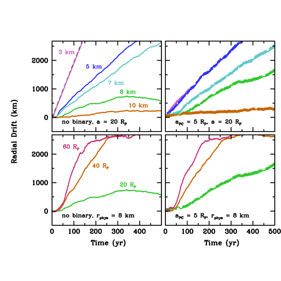
Figure 7: Migration of single satellites through a particle disk. Each trace shows the result of a simulation with either a single central point mass (left panels, with mass equal to the sum of $M_{P}$ and $M_{C}$) or a central Pluto-Charon binary with orbital separation of 5$R_{P}$. The legends give the physical radii of each satellite with $\rho=1$ g cm^-3; the legends also show the semimajor axis of the satellites’ initial orbit. The disk model has a total mass of $3\times 10^{20}$ g in a disk with surface density $\Sigma\propto a^{-1}$ extending in radius from $20R_{P}$ to $70R_{P}$. Planets migrate more commonly in the inward direction; however, random events can result in outward migration.

Figure 7 illustrates results for single satellites around a single central mass (left panels) and a central binary system (right panels). At $a=20$ $R_{P}$ (Fig. 7; upper left panel), satellites with $R\approx$ 1–4 km should open a gap and undergo fast migration (eqs. [11–12]). Satellites with $R=3$ km migrate at rates $\dot{a}\approx$ 20 km yr^-1, close to the rate predicted in eq. (13). As the satellite radius increases from 3 km to 5–10 km, the migration rate drops considerably. These larger satellites have too much inertia to maintain the fast radial drift rate. Larger satellites with $R\gtrsim$ 10 km migrate at rates close to predicted rates for gap migration (eq. [14]).

Migration rates also depend on the semimajor axis of the satellite (Fig. 7; lower left panel). When the velocity dispersion of the disk is fixed, it is harder for smaller satellites with $R$ = 3–4 km to open up a gap in the disk at larger $a$ than at smaller $a$ (eq. [11]). Thus, small satellites migrate much more slowly at large $a$. However, $R_{fast}$ also increases with $a$. Larger satellites migrate more rapidly at larger $a$ than at smaller $a$. For a larger satellite with $R=$ 8 km, the migration rate slows considerably from $a$ = 60 $R_{P}$ (roughly 20 km yr^-1) to $a$ = 40 $R_{P}$ (roughly 10 km yr^-1) to $a$ = 20 $R_{P}$ ($\lesssim$ 1 km yr^-1). The relative change in the migration rate follows theoretical predictions (eqs. [13–14]).

The presence of a central binary changes these results modestly (Fig. 7; right columns). The most obvious impact of the Pluto–Charon binary is the increased velocity dispersion of disk particles. Larger velocity dispersion reduces the effectiveness of torque exchange between the satellite and disk particles in the satellite’s corotation zone, making it more difficult for a satellite to open up a gap in the disk (eq. [11]). Thus, smaller satellites migrate more slowly around a binary. There is some evidence from the simulations that larger satellites may migrate more rapidly around a binary. In these cases, larger satellites first clear their corotation zone and halt their radial drift. As the simulation proceeds, stirring from the binary feeds some material into the corotation zone, commencing a kind of “attenuated” migration (Bromley & Kenyon, 2011b). We speculate that this behavior may allow larger objects to drift more quickly through a circumbinary disk.

Simulations with a variety of disk masses confirm these general trends. Under the right conditions in disks with masses larger than $\sim 10^{18}$ g, satellites with $R\approx$ 1–20 km can undergo fast, gap, or attenuated migration with rates ranging up to 20 km yr^-1. In lower mass disks, small satellites cannot clear the gap required to initiate fast migration. Although large satellites can form gaps in disks with $M_{d}\lesssim 10^{18}$ g, the minimum radius required to open a gap is larger than the maximum radius for fast migration. Thus, large satellites cannot migrate in the fast mode. Instead, these objects migrate a factor of ten more slowly in the gap migration mode.

To test whether the disk can circularize the orbits of small satellites, we derive predicted rates for 4–10 km objects in disks with $M_{d}=1-10\times 10^{17}$ g surrounding a single central object. For satellites in this size range, damping rates are independent of radius. The damping time scales with the disk mass:

$$t_{damp}\approx{e\over\dot{e}}\approx 10^{5}\left({10^{17}~{}{\rm g}\over M_{d}}\right)~{}{\rm yr}~{}.$$ (15)

Even in a low mass disk, damping times are comparable to the formation time for 4–10 km satellites.

Estimating damping rates for satellites orbiting a central binary is complicated by precession, orbital resonances, and other dynamical issues. For the small rates indicated by simulations with a single central object, accurate estimates require a substantial investment of cpu time. When the Pluto–Charon binary has a circular orbit, dynamical friction between the satellite and disk particles will still circularize the satellite’s orbit. In an eccentric Pluto–Charon binary, the damping time probably depends on the time scale for the disk and tides to circularize the binary. Because these processes act on similar time scales, deriving the circularization time for a satellite orbit is very cpu intensive and beyond the scope of this study.

3.5.3 Migration of Multiple Satellites

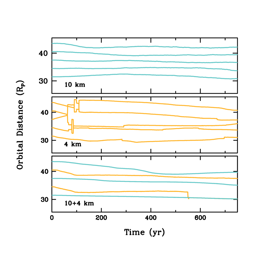
Figure 8: Migration of multiple satellites around a tight Pluto-Charon binary. The binary orbit and disk model are the same as in Figure 7, except that each set of five satellites is embedded in a 20$R_{P}$ annulus of disk particles. Each panel gives an example of the simulation output; the upper panel shows equal-mass 10 km satellites, while the middle panel tracks smaller 4 km bodies. In the former case, some radial drift occurs but does not lead to significant scattering or merging. The smaller satellites are more interactive; the middle panel shows an orbit crossing event. The lower panel illustrates differential migration in which a smaller body merges with a larger one.

To investigate whether ensembles of proto-satellites can migrate, we examine a second suite of simulations (Figure 8). Here, we maintain the same disk surface density distribution and focus on satellites with $R$ = 4 km or 10 km orbiting within a wide annulus spanning orbital distances of 35$R_{P}$ to 55$R_{P}$. Satellites and disk material orbit a compact Pluto–Charon binary with orbital separation $a$ = 5 $R_{P}$. For material at 35–55 $R_{P}$, stirring by the binary has a smaller impact than at 20 $R_{P}$.

The top panel of Figure 8 follows a simulation of five 10 km satellites initially evenly spaced in orbital separation. With typical Hill radii of 0.2 $R_{P}$, these satellites interact weakly among themselves. All have radii larger than $R_{fast}$; migration rates are slow. Modest scattering of disk particles yields some inward or outward motion and occasional stronger gravitational interactions among the satellites. However, these satellites are fairly stable over 1000 yr and longer timescales.

Simulations with ensembles of five 4 km objects produce more complicated outcomes. With much smaller Hill radii, these satellites interact very weakly among themselves. At the onset of each simulation, however, all begin to migrate in the fast mode. Some migrate inward; others migrate outward. When neighboring satellites migrate in the same direction, migration is limited by the stirred up wake of disk particles left behind by the first satellite to pass through that portion of the disk (Bromley & Kenyon, 2011b). Satellites do not cross these wakes. Thus, groups of small satellites migrating in the same direction drift radially inward/outward a small distance before the migration stalls.

Small satellites migrating in opposite directions lead to more interesting outcomes. Often, these satellites scatter one another, sometimes exchanging orbits (Fig. 8; middle panel). Depending on the sense of migration and the state of the disk after scattering, satellites may undergo multiple scattering events before settling down in roughly stable configurations within a stirred up disk. Sometimes, satellites merge. Because merged satellites are massive, they migrate more slowly and end up in a stable configuration. In our suite of simulations, mergers are less common ($\sim$ 10%) than scattering events.

Simulations with a mix of 4 km and 10 km satellites also lead to interesting outcomes (Fig. 8; lower panel). If a small satellite undergoing fast migration lies between two larger satellites, its larger migration rate guarantees that it will catch up to one of its slowly moving neighbors. When it does catch up, it may ‘bounce off’ the wake of its neighbor and begin migrating in the opposite direction. In roughly half of all interactions, the larger satellite either scatters or merges with the smaller satellite. If scattering places the small satellite on an orbit with a pericenter inside $a_{min}$, the central binary can eject the small satellite out of the system.

3.5.4 Summary of Migration Calculations

For satellites with $R\approx$ 4–10 km in a disk surrounding the Pluto–Charon system, migration is ubiquitous. In a cold, geometrically thin disk, satellites in this size range can undergo fast mode or slower, gap migration at rates very close to those predicted by analytic theory. These rates lead to significant radial motion, $\sim$ 1–10 $R_{P}$, on timescales comparable to the growth time of 1–10 km satellites, $\sim 10^{2}-10^{3}$ yr.

Interactions between the disk and the central binary can augment or reduce migration rates. Although changes to the rates are modest, smaller (larger) satellites generally migrate more slowly (rapidly). Changes are more significant closer to the binary, where the jitter of particle orbits in the disk modifies the number of particles in the corotation zone of a satellite. Thus, small (large) satellites which form closer to the binary are less (more) likely to migrate than satellites which form farther away from the binary.

Ensembles of migrating satellites produce a variety of interesting dynamical phenomena. In systems with several small satellites or a mix of large and small satellites, differential migration enables large-scale scattering events and satellite mergers. When scattering places a satellite on a orbit with a pericenter smaller than $a_{min}$, the central binary ejects the satellite from the system. Mergers among migrating satellites allow lower mass disks to produce more massive satellites.

The ability of satellites to migrate through an evolving disk depends on the ratio of the vertical scale height $H_{z}$ to the Hill radius $R_{H}$. When collisional damping dominates particle stirring, $H_{z}/R_{H}\lesssim$ 1. Satellites can open gaps in the disk and migrate at the nominal rates. In a disk dominated by particle stirring, $H_{z}/R_{H}\approx 3(a/20R_{P})^{1/2}$. When $H_{z}/R_{H}\gtrsim$ 1, satellites cannot open gaps in the disk. Migration is then ‘attenuated,’ with a rate smaller by a factor of roughly $(H_{z}/R_{H})^{3}\approx$ 30–100 at $a\approx$ 20–60 $R_{P}$ (Ida et al., 2000; Kirsh et al., 2009; Bromley & Kenyon, 2011b). Despite this reduction, the attenuated gap migration rate is still substantial, $\sim$ 1 $R_{P}$ every 10 Myr, similar to the time scale for tides and dynamical interactions to modify the semimajor axis of the binary orbit.

The ability of satellites to migrate efficiently also depends on the depletion rate of small particles in the disk. Small particles drive the migration of large particles. As particles grow from 0.1 km and smaller objects into 1 km and larger objects, the mass of the disk capable of driving migration declines. When the largest objects have $R\approx$ 1–5 km, most of the disk mass is in small objects. Thus, the large objects migrate at the nominal rate. Once the largest objects reach sizes of 10–30 km, small objects contain less than half of the initial disk mass. Migration is then slower than the nominal rate.

Scaling the migration rates derived in the simulations to the hotter disks expected from the coagulation and hybrid calculations in §3.4, satellites with radii similar to Kerberos and Styx may migrate significantly as they grow. Although larger satellites such as Nix and Hydra migrate more slowly, radial motion of a few Pluto radii seems likely after they reach their final sizes.

Although remnant particle disks with low masses, $\sim 10^{17}$ g, cannot drive migration on short time scales, they are effective in circularizing the orbits of satellites with sizes of 1–10 km. The time scale to circularize the orbit of a satellite is a factor of 10–100 times shorter than the time scale for tides to expand the orbit of the Pluto–Charon binary. Large final eccentricities, $e\approx$ 0.02–0.1, are a common feature in hybrid simulations of satellite formation (§3.4). Once satellites reach their final masses on time scales of $10^{4}-10^{5}$ yr, remnant disks with masses of $10^{16}-10^{17}$ g are ubiquitous. Thus, the migration simulations demonstrate that satellites embedded in a low mass disk will have the small eccentricities observed in the Pluto–Charon system.

This discussion suggests two plausible phases for migration in a circumbinary disk surrounding Pluto–Charon. During the early stages of the evolution, rapid migration of small satellites is possible when collisional damping dominates particle stirring. During this phase, growing satellites can migrate at least several Pluto radii. Later on, when stirring by newly-formed satellites dominates collisional damping, attenuated migration in a low mass disk slowly modifies satellite orbits as the inner binary expands. During this period, satellites may migrate much less than a Pluto radius, especially if the collisional cascade removes most of the small particles remaining in the disk.

4 DISCUSSION

Our analysis in §3 suggests that the steps outlined in §2 provide a reasonable path to the formation of small satellites close to their current positions within debris from the giant impact. This process begins (step 1) with the growth of Pluto-mass planets in a circumstellar disk of solid material. Once Plutos form, giant impacts are common (step three). During intervals between impacts (step two), Plutos capture $\sim 10^{19}$ g of debris. The debris has large $a$ and probably does not interact with material from the impact. Following impact (step 4), material ejected from the impact lies at $a\approx$ 20 $R_{P}$. In a reasonably massive disk composed of 0.1–1 km particles, angular momentum transfer from the binary to the ring and among ring particles spreads the ring to the current positions of the satellites on fairly short time scales. As the ring spreads, high velocity collisions diminish the sizes of the largest particles and remove mass from the ring. Eventually, collisional damping overcomes secular perturbations from the binary, enabling the growth of satellites within a broad ring. As satellites grow, they migrate through the ring. Although our calculations do not yield satellites at the same positions as Styx–Hydra, they yield satellites at similar positions. Often, stable satellites lie in approximate resonances.

Despite the plausibility of this picture, there are definite uncertainties. During the interval prior to impact, Pluto and Charon probably capture a modest amount of material. However, it is not clear whether any of this material can interact with debris from the impact. After impact, there is a broad range of likely values for the binary eccentricity and the properties of the ejecta. Within this range, it is not certain that collisions can damp velocities and redistribute angular momentum fast enough to overcome secular stirring, spread the ring into a disk, and enable the growth of smaller particles. Although it is plausible that a few large particles with $R\approx$ 1–10 km escape destruction during ring formation and serve as the seeds for large satellites (§3.4), they may be unable to flow out in an expanding ring of smaller objects. Even if satellites form within material in an expanded disk of material, they must survive the expansion of the Pluto–Charon binary. For satellites at $a\lesssim$ 30 $R_{P}$, survival seems unlikely (Peale et al., 2011). To survive at larger $a$, satellites must avoid interactions that destabilize their orbits.

Once a stable disk forms at $a\approx$ 15–70 $R_{P}$, our calculations yield testable predictions for the masses and orbital configurations of the Pluto–Charon satellites. The timescale for satellite growth depends on the properties of the binary and the ring of debris. In any configuration, there is a period where collisional damping must overcome tidal forcing from the central binary. Although we have not calculated this evolution in detail, our estimates in §3.3 imply a time scale of at least 1–10 yr. As this evolution proceeds, the ring probably loses a significant fraction of its initial mass. Once collisions calm the disk, the formation time for 1–10 km satellites is

$$t_{f}\approx 10^{3}\left({3\times 10^{19}~{}{\rm g}\over M_{d}}\right)\left({a\over 30R_{P}}\right)^{5/2}~{}{\rm yr}.$$ (16)

During oligarchic and chaotic growth, proto-satellites radially migrate through the leftover debris. Although proto-satellites cannot fall into the Pluto–Charon binary, satellites can traverse a substantial fraction of the circumbinary disk throughout chaotic growth. Migration can induce mergers among lower mass satellites, enabling more massive satellites to form in lower mass disks. Ensembles of satellites with similar masses migrate in step with one another, enabling satellites to find stable equilibrium orbits around Pluto–Charon.

Migration rates depend on the nature of the central object. Stirring by a central binary can heat the particle disk and slow migration of satellites with radii of $O(1)$ km. The binary may also increase migration rates of larger satellites. Migration is driven by the asymmetry of inward and outward satellite-disk scattering events. Compared to a single central mass, a binary preferentially disturbs a larger fraction of the orbits of the inwardly scattered disk particles and prevents their return to the satellite. We plan additional simulations to explore whether this possibility is sufficient to produce the derived changes in migration rates.

Migration rates are also sensitive to the mass of small objects remaining in the disk. When satellites reach sizes of 1–10 km, small particles still contain most of the mass. If collisional damping can maintain a small vertical scale height, satellites migrate 1–10 $R_{P}$ through the disk. As these satellites grow, they migrate more and more slowly due to the larger vertical scale height and smaller total mass in small particles. Eventually, migration stalls completely. Throughout this process, interactions between the satellites and the remnant disk of small particles circularize the orbits of the satellites.

Together with previous results from Youdin et al. (2012), our calculations indicate several conclusions about each satellite.

• The semimajor axis of Styx is almost as close as possible to the minimum stable circumbinary semimajor axis $a_{min}$. In our framework, Styx has a low mass because (i) the debris ring had less mass close to Pluto–Charon  (ii) it was scattered out of a more massive region of the ring by Nix or Hydra, or (iii) after formation at large $a$, it migrated into an innermost stable orbit.

• The orbit of Kerberos lies within a small stable region between the orbits of Nix and Hydra (Youdin et al., 2012). More massive satellites in this region are unstable. From the coagulation and migration calculations, Kerberos is a smaller remnant of the accretion process.

• The masses of Nix and Hydra are consistent with the coagulation models. The central cores of either satellite might have survived the giant impact and then accreted debris leftover from the impact. Alternatively, the satellites could form in a disk of small particles orbiting Pluto–Charon.

Aside from informing the next generation of numerical simulations for satellite formation, the New Horizons mission can test several predictions of our calculations.

• In our simulations, more massive disks generally produce fewer small satellites. Forming four (or more) satellites orbiting Pluto–Charon implies circumbinary disks with relatively small masses, $M_{d}\lesssim 3\times 10^{20}$ g. Together with numerical simulations of the orbital stability of the satellites (Youdin et al., 2012), these results require satellite albedos, $A\approx$ 0.4–1. This range for $A$ is similar to the measured $A\approx$ 0.5 for Pluto and Charon (see Marcialis et al., 1992; Roush et al., 1996; Brown, 2002; Buie et al., 2010a, b, and references therein) and much larger than the $A$ for many Kuiper belt objects (e.g., Stansberry et al., 2008; Brucker et al., 2009). Direct measurements of $A$ by New Horizons will test these constraints.

• All of the hybrid calculations leave several very small satellites orbiting within an extended disk of debris beyond the orbit of Hydra. The radii of typical leftovers – $R\lesssim$ 1–3 km – imply optical magnitudes of 28 or fainter. Testing this prediction is a challenge for Hubble Space Telescope (Showalter et al., 2011, 2012), but satellites this size or smaller are easily visible during the flyby of New Horizons. For objects with $R\approx$ 1–3 km, the most likely range of semimajor axes is $a\approx$ 70–90 $R_{P}$. Smaller satellites might have $a\approx$ 100–200 $R_{P}$. Both sets of small satellites should have small inclinations relative to the Pluto–Charon orbital plane, similar to the observed $i$ for the known satellites. If smaller particles in a leftover debris disk (see next item) have sufficient mass, these outer satellites should also have circular orbits. Smaller masses in leftovers imply larger $e$ for small outer satellites. We plan numerical calculations to test the longevity of these satellites in the tidal field of the Sun–Neptune system.

• Estimates for the spreading time in §3.3 suggest scattering will produce ensembles of smaller particles, $R\lesssim$ 0.01–10 m, in an extended disk well beyond the orbits of the known satellites. For a mass of $\sim 10^{15}$ g in leftover small particles with typical radius R, the predicted optical depth of the disk is $\tau_{l}\sim 10^{-10}R^{-1}$ at semimajor axes $a\approx$ 70–200 $R_{P}$. Larger (smaller) disk masses imply proportionately larger (smaller) optical depths. Although this mass is significant, the predicted optical depth is much smaller than the $\tau\lesssim 10^{-7}$ estimated for clouds of 1–100 $\mu$m particles produced by impacts of small Kuiper belt objects on the known satellites (Poppe & Horányi, 2011). New Horizons measurements of the optical depths of small particles surrounding the known satellites and at larger distances should place interesting constraints on the long-term evolution of the satellite system and its interactions with the Kuiper belt.

• Measuring the amount of material at $a\gtrsim$ 100 $R_{P}$ tests formalisms for the capture frequency (§3.2). In our estimates, most of the mass lies at large semimajor axes, $a\approx$ 1000 $R_{P}$. Failure to identify any material at $a\approx$ 100–1000 $R_{P}$ suggests that capture is less frequent than our estimates. In principle, the amount of material at these distances provides a measure of the capture efficiency.

• Composition data from New Horizons should also test the giant impact scenario. If the relative contamination from captured material (§3.2) or impacting Kuiper belt objects (e.g. Stern et al., 2006; Poppe & Horányi, 2011) is small, satellites should have roughly the same composition as Charon. The broad variety of physical characteristics among Kuiper belt objects (see Barucci et al., 2008) suggests that satellites with significant contributions of material from the Kuiper belt should have very different compositions from satellites grown from the debris of a giant impact (see also Stern, 2009). Thus, direct measurement of the compositions of individual satellites and gradients in the composition among any smaller satellites and debris should constrain scenarios for satellite formation.

• Observed shapes of satellites might also test formation models. In general, large fragments from the impact should be more irregular than satellites grown from a circumbinary disk/ring of much smaller particles (see Tanga et al., 2009a, b, and references therein).

To develop predicted configurations for the Pluto–Charon system during a New Horizons encounter, we ran $n$-body simulations of Pluto–Charon, the known small satellites, and several predicted satellites embedded within a disk of $0.5-2\times 10^{6}$ massless tracer particles. On $10^{2}$ yr time scales (roughly 5000 orbits of the inner binary), the larger satellites clear many tracers from their orbits (Fig. 9, left panel). On $10^{4}$ yr time scales, the four inner satellites clear most of the tracers from the inner disk (Fig. 9, right panel). Although the three outer satellites can clear tracers along their orbits, most tracers remain between satellite orbits in the outer disk.

On much longer (1–10 Myr) time scales, the inner satellites clear their orbits completely (see also Youdin et al., 2012). In the outer disk, a few small satellites with radii of a few km cannot clear more than a few hundred km around their orbits. Thus, many tracers remain. The predicted optical depth and extent of the disk at late times depends on (i) the number of small satellites beyond Hydra, (ii) the outcomes of collisions between small disk particles, and (iii) the amount of mass in small particles produced from recent impacts on the satellites (e.g., Stern, 2009; Poppe & Horányi, 2011) and capture from the Kuiper Belt. If (i) there are few small satellites, (ii) collisions damp and do not destroy small disk particles, and (iii) captures and impacts are common, we expect New Horizons to detect a modest disk of small particles with rings and gaps similar to those shown in the right panel of Fig 9). If, however, (i) there are many small satellites beyond Hydra’s orbit, (ii) collisions destroy small disk particles, and (iii) captures and impacts are relatively rare, the New Horizons encounter may reveal little or no disk material. Once New Horizons has mapped the Pluto–Charon system completely, improved numerical simulations will enable a more complete examination of the formation and history of the satellite system.

5 SUMMARY

We describe a theoretical framework for the origin of Pluto’s small satellites in the context of a giant impact that produces the Pluto–Charon binary (e.g., Canup, 2011). Our main results follow.

• Throughout the early history of the solar system, giant impacts capable of producing the Pluto–Charon binary have a frequency of 1 per 100–300 Myr. These impacts leave behind enough debris to enable satellite formation (Canup, 2011). Once the debris lies within a ring, angular momentum transport among ring particles may enable the ring to spread into a disk.

• In a ring or a disk of small particles, $R\lesssim$ 0.1 km, surrounding Pluto–Charon, satellites with $R\approx$ 10–80 km form rapidly on a time scale of $10^{3}-10^{4}$ yr. The formation time is similar to the migration time scale.

• After the impact, objects with $R\approx$ 1–10 km might survive collisional disruption during the ejection process. Calculations of disks with small particles and a few seeds produce fewer satellites with larger masses than calculations with small particles alone.

• Radial migration encourages mergers of small satellites within an evolving disk surrounding Pluto–Charon.

• Scattering events among differentially migrating satellites sometimes place objects on orbits with pericenters close to the central binary. Unless interactions with disk particles can damp the orbit, the Pluto–Charon binary ejects these satellites from the system.

• For identical masses of the central planet(s), the surrounding disk, and a small satellite embedded in the disk, migration rates around a binary planet differ slightly from those around a single planet. For Pluto–Charon, the drift rate of a satellite the size of Styx may be as high as 5 km yr^-1.

• The current number of small Pluto–Charon satellites strongly favors low mass disks (see also Youdin et al., 2012). In our calculations, disks with masses $M_{d}\approx 3-10\times 10^{19}$ g have the best chance at producing 3–5 satellites with orbital semimajor axes $a\approx$ 40–60 $R_{P}$. Matching observations requires Pluto’s satellites to have albedos $A\approx$ 0.4–1. New Horizons data will test this prediction.

• Model satellites produced in formation calculations have orbital $i$ close to those observed, but the typical $e$ is generally too large. Orbital migration can reduce $e$ to acceptable levels.

• The calculations predict a few very small, $R\lesssim$ 1–3 km, satellites and an extended disk of even smaller particles, $R\approx$ 1–100 cm, beyond the current orbit of Hydra. Detecting these satellites and the disk from the ground is very challenging. If they are present, New Horizons should detect them easily.

Our results demonstrate that numerical calculations can produce simulated satellite systems with properties reasonably close to those observed. Prior to the New Horizons flyby of Pluto–Charon, we expect to refine the predictions considerably. Once New Horizons probes the masses, orbital architecture, and composition of the Pluto–Charon binary, a rich interplay between the data and the numerical simulations will enable a much more robust theory for the formation of satellites (planets) in binary planetary (stellar) systems.

We acknowledge generous allotments of computer time on the NASA ‘discover’ cluster and the SI ‘hydra’ cluster. Advice and comments from M. Geller and A. Youdin greatly improved our presentation. We thank two anonymous referees for thoughtful comments that honed our analysis. Portions of this project were supported by the NASA Astrophysics Theory and Origins of Solar Systems programs through grant NNX10AF35G and the NASA Outer Planets Program through grant NNX11AM37G.

Figure 9: Predicted configuration for the Pluto–Charon system. The Pluto–Charon binary (represented by the two largest white disks), the four small satellites – Styx, Nix, Kerberos, and Hydra (represented by the four small white disks), and three smaller satellites (represented by the green disks) lie within an extended ensemble of solid particles shown as small blue dots. Left panel: System configuration after $10^{2}$ yr of a computer simulation with two million massless tracer particles surrounding the known and predicted moons. Right panel: System configuration after $10^{4}$ yr of a computer simulation with 0.5 million massless tracer particles. On short times scales, satellites remove tracer particles along their orbits. On long time scales, satellites remove nearly all tracers in the inner disk; low mass satellites in the outer disk begin to clear their orbits. On time scales of $\gtrsim 10^{6}$ yr, satellites will clear the inner disk of small particles (see also Youdin et al., 2012); collisional erosion and scattering will probably remove most of the particles in the outer disk.

References

- Agnor et al. (1999) Agnor, C. B., Canup, R. M., & Levison, H. F. 1999, Icarus, 142, 219
- Asphaug et al. (2006) Asphaug, E., Agnor, C. B., & Williams, Q. 2006, Nature, 439, 155
- Barucci et al. (2008) Barucci, M. A., Boehnhardt, H., Cruikshank, D. P., & Morbidelli, A. 2008, The Solar System Beyond Neptune, ed. Barucci, M. A., Boehnhardt, H., Cruikshank, D. P., & Morbidelli, A. (University of Arizona Press, Tucson, AZ)
- Benz & Asphaug (1999) Benz, W., & Asphaug, E. 1999, Icarus, 142, 5
- Brahic (1976) Brahic, A. 1976, Journal of Computational Physics, 22, 171
- Brahic (1977) —. 1977, A&A, 54, 895
- Bromley & Kenyon (2006) Bromley, B. C., & Kenyon, S. J. 2006, AJ, 131, 2737
- Bromley & Kenyon (2011a) —. 2011a, ApJ, 731, 101
- Bromley & Kenyon (2011b) —. 2011b, ApJ, 735, 29
- Bromley & Kenyon (2013) —. 2013, ApJ, 764, 192
- Brown (2002) Brown, M. E. 2002, Annual Review of Earth and Planetary Sciences, 30, 307
- Brucker et al. (2009) Brucker, M. J., Grundy, W. M., Stansberry, J. A., Spencer, J. R., Sheppard, S. S., Chiang, E. I., & Buie, M. W. 2009, Icarus, 201, 284
- Buie et al. (2006) Buie, M. W., Grundy, W. M., Young, E. F., Young, L. A., & Stern, S. A. 2006, AJ, 132, 290
- Buie et al. (2010a) —. 2010a, AJ, 139, 1117
- Buie et al. (2010b) —. 2010b, AJ, 139, 1128
- Burns et al. (1979) Burns, J. A., Lamy, P. L., & Soter, S. 1979, Icarus, 40, 1
- Canup (2005) Canup, R. M. 2005, Science, 307, 546
- Canup (2011) —. 2011, AJ, 141, 35
- Canup & Ward (2002) Canup, R. M., & Ward, W. R. 2002, AJ, 124, 3404
- Chambers (2001) Chambers, J. E. 2001, Icarus, 152, 205
- Chambers (2013) —. 2013, Icarus, 224, 43
- Chambers & Wetherill (1998) Chambers, J. E., & Wetherill, G. W. 1998, Icarus, 136, 304
- Charnoz et al. (2010) Charnoz, S., Salmon, J., & Crida, A. 2010, Nature, 465, 752
- Charnoz et al. (2011) Charnoz, S., et al. 2011, Icarus, 216, 535
- Chiang & Youdin (2010) Chiang, E., & Youdin, A. N. 2010, Annual Review of Earth and Planetary Sciences, 38, 493
- Christy & Harrington (1978) Christy, J. W., & Harrington, R. S. 1978, AJ, 83, 1005
- Cionco & Brunini (2002) Cionco, R. G., & Brunini, A. 2002, MNRAS, 334, 77
- Dobrovolskis et al. (1997) Dobrovolskis, A. R., Peale, S. J., & Harris, A. W. 1997, Dynamics of the Pluto-Charon Binary, ed. S. A. Stern & D. J. Tholen, 159
- Dohnanyi (1969) Dohnanyi, J. S. 1969, J. Geophys. Res., 74, 2531
- Dominik & Decin (2003) Dominik, C., & Decin, G. 2003, ApJ, 598, 626
- Durda & Stern (2000) Durda, D. D., & Stern, S. A. 2000, Icarus, 145, 220
- Estrada & Mosqueira (2006) Estrada, P. R., & Mosqueira, I. 2006, Icarus, 181, 486
- Farinella et al. (1979) Farinella, P., Milani, A., Nobili, A. M., & Valsecchi, G. B. 1979, Moon and Planets, 20, 415
- Goldreich et al. (2002) Goldreich, P., Lithwick, Y., & Sari, R. 2002, Nature, 420, 643
- Goldreich et al. (2004) —. 2004, ARA&A, 42, 549
- Goldreich & Tremaine (1982) Goldreich, P., & Tremaine, S. 1982, ARA&A, 20, 249
- Goldreich & Tremaine (1978) Goldreich, P., & Tremaine, S. D. 1978, Icarus, 34, 227
- Greenberg et al. (1984) Greenberg, R., Weidenschilling, S. J., Chapman, C. R., & Davis, D. R. 1984, Icarus, 59, 87
- Hahn & Malhotra (1999) Hahn, J. M., & Malhotra, R. 1999, AJ, 117, 3041
- Hayashi (1981) Hayashi, C. 1981, Progress of Theoretical Physics Supplement, 70, 35
- Heppenheimer (1974) Heppenheimer, T. A. 1974, Icarus, 22, 436
- Holman & Wiegert (1999) Holman, M. J., & Wiegert, P. A. 1999, AJ, 117, 621
- Hornung et al. (1985) Hornung, P., Pellat, R., & Barge, P. 1985, Icarus, 64, 295
- Ida et al. (2000) Ida, S., Bryden, G., Lin, D. N. C., & Tanaka, H. 2000, ApJ, 534, 428
- Kennedy & Wyatt (2011) Kennedy, G. M., & Wyatt, M. C. 2011, MNRAS, 412, 2137
- Kenyon (2002) Kenyon, S. J. 2002, PASP, 114, 265
- Kenyon & Bromley (2001) Kenyon, S. J., & Bromley, B. C. 2001, AJ, 121, 538
- Kenyon & Bromley (2002) —. 2002, AJ, 123, 1757
- Kenyon & Bromley (2004a) —. 2004a, AJ, 127, 513
- Kenyon & Bromley (2004b) —. 2004b, ApJ, 602, L133
- Kenyon & Bromley (2004c) —. 2004c, AJ, 128, 1916
- Kenyon & Bromley (2005) —. 2005, AJ, 130, 269
- Kenyon & Bromley (2006) —. 2006, AJ, 131, 1837
- Kenyon & Bromley (2008) —. 2008, ApJS, 179, 451
- Kenyon & Bromley (2010) —. 2010, ApJS, 188, 242
- Kenyon & Bromley (2012) —. 2012, AJ, 143, 63
- Kenyon et al. (2008) Kenyon, S. J., Bromley, B. C., O’Brien, D. P., & Davis, D. R. 2008, in The Solar System Beyond Neptune, ed. Barucci, M. A., Boehnhardt, H., Cruikshank, D. P., & Morbidelli, A. (University of Arizona Press, Tucson, AZ), 293–313
- Kenyon & Luu (1998) Kenyon, S. J., & Luu, J. X. 1998, AJ, 115, 2136
- Kenyon & Luu (1999) —. 1999, AJ, 118, 1101
- Kirsh et al. (2009) Kirsh, D. R., Duncan, M., Brasser, R., & Levison, H. F. 2009, Icarus, 199, 197
- Kobayashi & Tanaka (2010) Kobayashi, H., & Tanaka, H. 2010, Icarus, 206, 735
- Kokubo & Ida (1996) Kokubo, E., & Ida, S. 1996, Icarus, 123, 180
- Kokubo & Ida (2002) —. 2002, ApJ, 581, 666
- Kominami & Ida (2002) Kominami, J., & Ida, S. 2002, Icarus, 157, 43
- Kominami & Ida (2004) —. 2004, Icarus, 167, 231
- Lee & Peale (2006) Lee, M. H., & Peale, S. J. 2006, Icarus, 184, 573
- Leinhardt et al. (2010) Leinhardt, Z. M., Marcus, R. A., & Stewart, S. T. 2010, ApJ, 714, 1789
- Leinhardt & Stewart (2009) Leinhardt, Z. M., & Stewart, S. T. 2009, Icarus, 199, 542
- Leinhardt & Stewart (2012) —. 2012, ApJ, 745, 79
- Leinhardt et al. (2008) Leinhardt, Z. M., Stewart, S. T., & Schultz, P. H. 2008, in The Solar System Beyond Neptune, ed. Barucci, M. A., Boehnhardt, H., Cruikshank, D. P., & Morbidelli, A. (University of Arizona Press, Tucson, AZ), 195–211
- Lin & Papaloizou (1979a) Lin, D. N. C., & Papaloizou, J. 1979a, MNRAS, 188, 191
- Lin & Papaloizou (1979b) —. 1979b, MNRAS, 186, 799
- Lin & Papaloizou (1986a) —. 1986a, ApJ, 307, 395
- Lin & Papaloizou (1986b) —. 1986b, ApJ, 309, 846
- Lissauer (1987) Lissauer, J. J. 1987, Icarus, 69, 249
- Lithwick & Wu (2008) Lithwick, Y., & Wu, Y. 2008, ArXiv e-prints
- Lunine & Stevenson (1982) Lunine, J. I., & Stevenson, D. J. 1982, Icarus, 52, 14
- Lynden-Bell & Pringle (1974) Lynden-Bell, D., & Pringle, J. E. 1974, MNRAS, 168, 603
- Malhotra (1993) Malhotra, R. 1993, Nature, 365, 819
- Marcialis et al. (1992) Marcialis, R. L., Lebofsky, L. A., Disanti, M. A., Fink, U., Tedesco, E. F., & Africano, J. 1992, AJ, 103, 1389
- Martin & Lubow (2011) Martin, R. G., & Lubow, S. H. 2011, MNRAS, 413, 1447
- McKinnon (1989) McKinnon, W. B. 1989, ApJ, 344, L41
- Morbidelli et al. (2008) Morbidelli, A., Levison, H. F., & Gomes, R. 2008, in The Solar System Beyond Neptune, ed. Barucci, M. A., Boehnhardt, H., Cruikshank, D. P., & Morbidelli, A. (The University of Arizona Press), 275–292
- Moriwaki & Nakagawa (2004) Moriwaki, K., & Nakagawa, Y. 2004, ApJ, 609, 1065
- Mosqueira et al. (2010) Mosqueira, I., Estrada, P., & Turrini, D. 2010, Space Sci. Rev., 153, 431
- Mosqueira & Estrada (2003a) Mosqueira, I., & Estrada, P. R. 2003a, Icarus, 163, 198
- Mosqueira & Estrada (2003b) —. 2003b, Icarus, 163, 232
- Murray & Dermott (1999) Murray, C. D., & Dermott, S. F. 1999, Solar system dynamics (Princeton: Princeton University Press)
- Nagasawa et al. (2005) Nagasawa, M., Lin, D. N. C., & Thommes, E. 2005, ApJ, 635, 578
- Nelson & Papaloizou (2004) Nelson, R. P., & Papaloizou, J. C. B. 2004, MNRAS, 350, 849
- Noll et al. (2008) Noll, K. S., Grundy, W. M., Chiang, E. I., Margot, J.-L., & Kern, S. D. 2008, in The Solar System Beyond Neptune, ed. Barucci, M. A., Boehnhardt, H., Cruikshank, D. P., & Morbidelli, A. (The University of Arizona Press: University of Arizona Press, Tucson, AZ), 345–363
- O’Brien & Greenberg (2003) O’Brien, D. P., & Greenberg, R. 2003, Icarus, 164, 334
- Ogihara & Ida (2012) Ogihara, M., & Ida, S. 2012, ApJ, 753, 60
- Ohtsuki (1992) Ohtsuki, K. 1992, Icarus, 98, 20
- Ohtsuki et al. (2002) Ohtsuki, K., Stewart, G. R., & Ida, S. 2002, Icarus, 155, 436
- Ormel et al. (2012) Ormel, C. W., Ida, S., & Tanaka, H. 2012, ApJ, 758, 80
- Paardekooper et al. (2012) Paardekooper, S.-J., Leinhardt, Z. M., Thébault, P., & Baruteau, C. 2012, ApJ, 754, L16
- Peale (1999) Peale, S. J. 1999, ARA&A, 37, 533
- Peale et al. (2011) Peale, S. J., Cheng, W. H., & Lee, M. H. 2011, in EPSC-DPS Joint Meeting 2011, 665
- Pires dos Santos et al. (2012) Pires dos Santos, P. M., Morbidelli, A., & Nesvorný, D. 2012, Celestial Mechanics and Dynamical Astronomy, 114, 341
- Poppe & Horányi (2011) Poppe, A., & Horányi, M. 2011, Planet. Space Sci., 59, 1647
- Pringle (1991) Pringle, J. E. 1991, MNRAS, 248, 754
- Rafikov (2001) Rafikov, R. R. 2001, AJ, 122, 2713
- Rafikov (2013) —. 2013, ApJ, 764, L16
- Rosenblatt & Charnoz (2012) Rosenblatt, P., & Charnoz, S. 2012, Icarus, 221, 806
- Roush et al. (1996) Roush, T. L., Cruikshank, D. P., Pollack, J. B., Young, E. F., & Bartholomew, M. J. 1996, Icarus, 119, 214
- Ruskol (1961) Ruskol, E. L. 1961, Soviet Ast., 4, 657
- Ruskol (1963) —. 1963, Soviet Ast., 7, 221
- Ruskol (1972) —. 1972, Soviet Ast., 15, 646
- Safronov (1969) Safronov, V. S. 1969, Evoliutsiia doplanetnogo oblaka. (Evolution of the Protoplanetary Cloud and Formation of the Earth and Planets), Nauka, Moscow [Translation 1972, NASA TT F-677] (Nauka:Moscow)
- Salmon et al. (2010) Salmon, J., Charnoz, S., Crida, A., & Brahic, A. 2010, Icarus, 209, 771
- Sasaki et al. (2010) Sasaki, T., Stewart, G. R., & Ida, S. 2010, ApJ, 714, 1052
- Scholl et al. (2007) Scholl, H., Marzari, F., & Thébault, P. 2007, MNRAS, 380, 1119
- Showalter et al. (2013) Showalter, M., et al. 2013, in EGU General Assembly Conference Abstracts, Vol. 15, EGU General Assembly Conference Abstracts, 13786
- Showalter et al. (2011) Showalter, M. R., Hamilton, D. P., Stern, S. A., Weaver, H. A., Steffl, A. J., & Young, L. A. 2011, IAU Circ., 9221, 1
- Showalter et al. (2012) Showalter, M. R., et al. 2012, IAU Circ., 9253, 1
- Sicardy et al. (2006) Sicardy, B., et al. 2006, Nature, 439, 52
- Stansberry et al. (2008) Stansberry, J., Grundy, W., Brown, M., Cruikshank, D., Spencer, J., Trilling, D., & Margot, J.-L. 2008, in The Solar System Beyond Neptune, ed. Barucci, M. A., Boehnhardt, H., Cruikshank, D. P., & Morbidelli, A. (University of Arizona Press, Tucson, AZ), 161–179
- Stern (1991) Stern, S. A. 1991, Icarus, 90, 271
- Stern (1995) —. 1995, AJ, 110, 856
- Stern (2008) —. 2008, Space Sci. Rev., 140, 3
- Stern (2009) —. 2009, Icarus, 199, 571
- Stern & Colwell (1997) Stern, S. A., & Colwell, J. E. 1997, AJ, 114, 841
- Stern et al. (2006) Stern, S. A., et al. 2006, Nature, 439, 946
- Suetsugu & Ohtsuki (2013) Suetsugu, R., & Ohtsuki, K. 2013, MNRAS, 431, 1709
- Suetsugu et al. (2011) Suetsugu, R., Ohtsuki, K., & Tanigawa, T. 2011, AJ, 142, 200
- Süli & Zsigmond (2009) Süli, Á., & Zsigmond, Z. 2009, MNRAS, 398, 2199
- Tanaka & Ida (1996) Tanaka, H., & Ida, S. 1996, Icarus, 120, 371
- Tanga et al. (2009a) Tanga, P., Hestroffer, D., Delbò, M., & Richardson, D. C. 2009a, Planet. Space Sci., 57, 193
- Tanga et al. (2009b) Tanga, P., et al. 2009b, ApJ, 706, L197
- Tholen et al. (2008) Tholen, D. J., Buie, M. W., Grundy, W. M., & Elliott, G. T. 2008, AJ, 135, 777
- Toth (1999) Toth, I. 1999, Icarus, 141, 420
- Tsukamoto & Makino (2007) Tsukamoto, Y., & Makino, J. 2007, ApJ, 669, 1316
- Ward (1997) Ward, W. R. 1997, Icarus, 126, 261
- Ward & Canup (2006) Ward, W. R., & Canup, R. M. 2006, Science, 313, 1107
- Ward & Canup (2010) —. 2010, AJ, 140, 1168
- Weaver et al. (2006) Weaver, H. A., et al. 2006, Nature, 439, 943
- Weidenschilling (1977) Weidenschilling, S. J. 1977, Ap&SS, 51, 153
- Weidenschilling (1989) —. 1989, Icarus, 80, 179
- Weidenschilling (2002) —. 2002, Icarus, 160, 212
- Weidenschilling et al. (1997) Weidenschilling, S. J., Spaute, D., Davis, D. R., Marzari, F., & Ohtsuki, K. 1997, Icarus, 128, 429
- Wetherill & Stewart (1989) Wetherill, G. W., & Stewart, G. R. 1989, Icarus, 77, 330
- Wetherill & Stewart (1993) —. 1993, Icarus, 106, 190
- Williams & Wetherill (1994) Williams, D. R., & Wetherill, G. W. 1994, Icarus, 107, 117
- Winter et al. (2010) Winter, S. M. G., Winter, O. C., Guimarães, A. H. F., & Silva, M. R. 2010, MNRAS, 404, 442
- Wyatt (2008) Wyatt, M. C. 2008, ARA&A, 46, 339
- Wyatt et al. (1999) Wyatt, M. C., Dermott, S. F., Telesco, C. M., Fisher, R. S., Grogan, K., Holmes, E. K., & Piña, R. K. 1999, ApJ, 527, 918
- Youdin (2011) Youdin, A. N. 2011, ApJ, 731, 99
- Youdin & Kenyon (2012) Youdin, A. N., & Kenyon, S. J. 2012, ArXiv e-prints
- Youdin et al. (2012) Youdin, A. N., Kratter, K. M., & Kenyon, S. J. 2012, ArXiv e-prints
- Young & Binzel (1994) Young, E. F., & Binzel, R. P. 1994, Icarus, 108, 219
- Young et al. (2007) Young, E. F., Young, L. A., & Buie, M. 2007, in Bulletin of the American Astronomical Society, Vol. 39, AAS/Division for Planetary Sciences Meeting Abstracts #39, 541