Department of Physics and Astronomy
Rutgers University
Piscataway, NJ 08854
Surveying Extended GMSB Models with GeV
Abstract
In order to achieve maximal stop mixing and GeV, we consider extensions of minimal GMSB that include marginal MSSM-messenger superpotential interactions. Using a new approach to analytic continuation in superspace, we derive general formulas for the soft masses in the presence of such interactions, correctly taking into account the role of MSSM-messenger mixing in a general framework for the first time. We classify and catalog all possible such interactions consistent with perturbative unification, and we survey the impact of turning on one interaction at a time, from the point of view of fine tuning, spectrum and phenomenology. We find that the best models are fine-tuned to the sub-percent level and are accessible at the 14 TeV LHC. We highlight potential search strategies that can probe the characteristic spectra of these models.
1 Introduction
Recently, both the ATLAS and CMS experiments have announced the discovery of a Standard Model-like Higgs with GeV Aad:2012tfa ; Chatrchyan:2012ufa . This exciting result provides interesting hints and challenges for physics beyond the Standard Model. Supersymmetry (SUSY), long the preferred solution to the hierarchy problem, is highly constrained by this value of the Higgs mass. In particular, in the MSSM, large radiative corrections from stop/top loops are needed for GeV (see e.g. Hall:2011aa ; Heinemeyer:2011aa ; Arbey:2011ab ; Draper:2011aa ; Carena:2011aa ). These contributions can arise either through extremely heavy, unmixed stops ( TeV), or through lighter stops with maximal mixing Casas:1994us ; Carena:1995bx ; Haber:1996fp :
| (1.1) |
By transplanting the stops from 1 to 10 TeV, the theory grows two orders of magnitude more tuned. Since such a tuned model has little hope for ever being observed at the LHC, we will focus on generating the light, mixed stops in this work.
Large -terms are essential for obtaining a heavy Higgs with lighter stops. This presents a special challenge for models of gauge mediated SUSY breaking (GMSB) (for a review and original references, see Giudice:1998bp ), which are strongly motivated by the SUSY flavor problem, but do not produce -terms at the messenger scale. Large -terms can be generated through RG running driven by a heavy gluino Draper:2011aa , but this requires a very large messenger scale and, again, reduces both the naturalness and the likelihood of observing any superpartners at the LHC. (See also Ajaib:2012vc , which studies these issues in the context of minimal GMSB and reaches the same conclusions.)
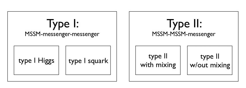
In this paper, we will instead study models which directly generate large at low messenger scales through marginal superpotential interactions between MSSM and messenger superfields. We will focus on fully calculable models of perturbative messengers coupled to SUSY-breaking spurions. There are then two types of marginal interaction terms: MSSM-messenger-messenger couplings, and MSSM-MSSM-messenger couplings. We will refer to these couplings as type I and type II couplings, respectively. It is useful to further divide the type I couplings into two distinct subclasses, those in which the MSSM superfield participating in the interaction is a Higgs, and those in which it is a squark.
It is also useful to distinguish between couplings which give rise to mixing between the MSSM and messenger fields and couplings which do not. A prime example of a model with MSSM-messenger mixing is the model, where is a messenger with the same quantum numbers as . Other similar examples include ( mixing with ) and ( mixing with ). Such models have been studied by many authors in the literature, including ChackoPonton ; Shadmi:2011hs ; Evans:2011bea ; Jelinski:2011xe ; Evans:2012hg ; Albaid:2012qk ; Abdullah:2012tq ; Perez:2012mj ; Endo:2012rd . We only consider mixing in type II interactions, as the messengers in type I interactions can always be charged with a parity symmetry to forbid mixing.
Fig. 1 displays this classification of models – into type I Higgs, type I squark, type II with mixing and type II without mixing. This classification will form the basis for the results presented in this paper. A primary goal of this work will be to describe models within these different categories and their general features with regards to fine tuning and phenomenology.
The main theoretical challenge facing calculable models for large -terms is something that was dubbed the problem in CraigShih (see also Craig:2013wga for a recent discussion in a more general context). In direct analogy to the problem, models for -terms tend to also generate one-loop soft mass-squareds. Such large soft masses would be disastrous for naturalness and/or electroweak symmetry breaking (EWSB). As shown in CraigShih (following Giudice:2007ca ), spurion models which avoid the problem must be of the minimal gauge mediation (MGM) type:
| (1.2) |
in which all mass-scales in the messenger sector (consisting here of and ) originate from a single spurion with . All of the models that we consider in this paper are assumed to have a messenger sector of this form.
Although -terms are commonly viewed as trilinear soft terms, they actually arise as bilinear terms between the MSSM fields and their -components:
| (1.3) |
After integrating out the -components, this becomes with
| (1.4) |
In order to generate , it is mandatory that either , , or participate in the direct interactions with the messengers. In CraigShih , only couplings to messengers were considered, since this automatically preserves minimal flavor violation (MFV), one of the best features of gauge mediation. However, these models suffer from the residual “little problem” CraigShih : by integrating out in (1.3), an irreducible contribution is generated. Since TeV is required for maximal mixing and GeV, this results in an irreducible fine tuning at the level in these models.
Motivated by these considerations, we will broaden the scope of CraigShih and survey the complete class of spurion-messenger models for large , including also non-MFV couplings involving and . As expected, these squark-type couplings result in far less fine-tuning than the Higgs-type couplings, since they do not generate a little problem. For simplicity, and to minimize flavor changing effects, we consider scenarios with only a single coupling introduced between MSSM and messenger fields. This structure may seem unrealistic; however, it is technically natural and facilitates focus on the “best-case scenarios.” By restricting the models to complete messenger multiplets and requiring perturbative gauge couplings up to the GUT scale, only a finite and manageable list of couplings is permitted. Under these assumptions, there are a total of 31 couplings. The complete list of these can be found in table 1.
For computing the soft masses in these models, general formulas were derived in ChackoPonton using wavefunction renormalization and the technique of “analytic continuation into superspace” Giudice:1997ni . These formulas are cast in terms of anomalous dimensions and beta functions of non-holomorphic couplings, and they are sufficient for all type I and most type II models. However, one runs into numerous complications when attempting to apply them to type II models with mixing between MSSM and messenger superfields (such as the model described above). The problem stems from crucial assumption made in ChackoPonton that the wavefunctions are continuous through the messenger threshold. This proves to be incompatible with standard conventions for the beta functions and anomalous dimensions (e.g. those in MartinVaughn ). Attempting to substitute standard beta functions and anomalous dimensions into the general formulas of ChackoPonton , as many in the literature have done, leads to incorrect results.111While one can correctly apply the formulas of ChackoPonton in the mixed type II case by using non-standard beta functions and anomalous dimensions (see Evans:2012hg ), this has only been performed in one specific model, and standardized formulas do not exist. In fact, we have found these complications to be so insidious that nearly every paper that studies models with MSSM-messenger mixing contains erroneous formulas.
Faced with many incorrect results and an enormous amount of confusion in the literature, we will devote section 2 to describing a new approach to deriving the soft masses using wavefunction renormalization. The main idea of our new approach is to obtain the wavefunctions by direct integration in a manifestly holomorphic scheme, rather than first utilizing the beta functions for the non-holomorphic couplings, as done in ChackoPonton . This results in a conceptually cleaner approach, which circumvents the difficulties of ChackoPonton and leads to fully general, correct formulas which can be applied uniformly to all models, whether mixing is present or not. In appendix A, we provide many checks of our results for the model described above, and illustrate the complications that arise in type II models with mixing, using this concrete example.
With the correct and fully general formulas for the soft masses in hand, we will compute the soft masses at the messenger scale for each model in table 1, and then investigate the parameter space where GeV. For such points in the viable parameter space, we will survey the phenomenology and fine tuning. In order to quantify tuning in these models, we utilize a tuning measure, , that is based on the Giudice-Barbieri tuning measure GiudiceBarbieri , but with a slightly unconventional choice of underlying parameters. This choice is made to ensure that the tuning measure captures all sensitivities successfully, does not introduce artificial tuning, and assigns comparable weight to uncorrelated contributions which cancel against one another. A detailed discussion and definition of the tuning measure is provided in section 3 and appendix B.
We find that with the GeV constraint, the least-tuned spectra can be accessible at the 14 TeV LHC, but are generally beyond the reach at 8 TeV. This suggests an intriguing possibility: that the failure to find superpartners so far at the LHC could actually be a consequence of GeV, rather than a separate issue.
Here is a synopsis of our results for each kind of model:
-
•
We confirm that the type I Higgs models (some of which have been studied before in Jelinski:2011xe ; Kang:2012ra ; CraigShih ; Albaid:2012qk ) are indeed fine-tuned at the level of because of the little problem. The spectra of the best points across the different models are rather similar. However, the prospects for observing these models at the LHC are rather pessimistic because all of the colored objects tend to be quite heavy. Some spectra do possess a light wino which could be produced at the LHC, but this is the exception rather than the norm. These spectra all exhibit slepton co-NLSPs with roughly 250-450 GeV masses – within the range that an ILC could discover.
-
•
On the other hand, in the type I squark models, there is no little problem, so these models are considerably less fine tuned. To the best of our knowledge, these models have never been studied in detail before. All of these models possess points of relatively low tuning, with . However, as these models are not manifestly MFV, they can in principle conflict with flavor physics constraints from precision experiment. For the purposes of this work, we adopt an agnostic stance toward flavor (e.g. we assume perfect alignment) and simply aim to show that the type I squark models are promising from a tuning point of view. Discussions of flavor physics in these models will be deferred for future work paperwithArun . The LHC phenomenology of these models is more promising. Often, there is an accessible stop (and sbottom in models) with slepton co-NLSPs, sometimes with a bino between the two states. Alternatively, some of the regions of lower tuning have gluinos and squarks light enough to be produced at 14 TeV.
-
•
There are five type II models with mixing, and they have been studied in various guises in ChackoPonton ; Shadmi:2011hs ; Evans:2011bea ; Jelinski:2011xe ; Evans:2012hg ; Albaid:2012qk ; Abdullah:2012tq ; Perez:2012mj ; Endo:2012rd . In three of these terms the interaction is top-Yukawa-like (, and ), and in two of them it is bottom-Yukawa-like ( and ). The latter receive no appreciable influence from mixing, but they are more constrained by tachyons and/or EWSB, so they manifest with poor tuning. Conversely, the top-Yukawa-like terms are especially interesting as is enhanced by receiving contributions from two sources (1.4). This enhancement is so effective that the mixed model contains the points with the least tuning out of any model studied in this work. Though inferior to the best regions of all type I squark models, the and models have regions with lower tuning than the type I Higgs models and the rest of the type II models. The regions of least tuning in the model are experimentally excluded by existing LHC searches because they have light gluinos and first-generation squarks. The other top-Yukawa-like models have spectra with gluinos and first generation squarks which will be accessible at 14 TeV running. Other production avenues, especially promising at an ILC, include very light slepton co-NLSPs and light Higgsinos entering at several hundred GeV.
-
•
Most of the type II models without mixing (see Kim:2005qb ; Joaquim:2006mn ; Albaid:2012qk ; Kim:2012vz for some examples) are extremely tuned. These models tend to either suffer from the same issues as the type I Higgs models, or introduce additional tachyons which place the model in tiny corners of viable parameter space. However, the model has regions of slightly lower tuning. Additionally, these models depart from the slepton co-NLSP phenomenology of the type I models and will often have a bino NLSP. Gluinos accessible at 14 TeV could lead to exciting phenomenology.
Our paper is outlined as follows: In section 2, we discuss the complications which arise when using analytic continuation in superspace to derive soft parameters in models with MSSM-messenger mixing. We then present a new, completely general framework for deriving messenger scale soft parameters in the presence of any MSSM-messenger interactions. In section 3, we catalog and survey the parameter space of the 31 possible couplings. Details are provided in a series of subsections for type I Higgs, type I squark, type II mixed and type II unmixed models. We discuss the phenomenology of the models with the least tuning in section 4. Section 5 contains a summary and discussion of future directions. We devote appendix A to validating the formulas of section 2 through multiple methods. The fine-tuning measure utilized throughout this work is detailed in appendix B.
Note added: while this paper was in preparation, Byakti:2013ti appeared which overlaps partially with section 3 of our work. This paper also creates a catalog of the different models of MSSM-messenger interactions for large . We note that their classification scheme differs from ours; our catalog contains several additional couplings absent from their study, namely , , , , as well as all couplings containing an adjoint, ; and their formulas, being based on those of ChackoPonton , neglect a proper treatment of MSSM-messenger mixing.
2 A New Calculation of the Soft Spectrum
2.1 Problems with the existing derivation
In this section, we present a new method for calculating the soft spectrum induced by MSSM-messenger interactions via analytic continuation in superspace. The current state of the art (prior to this work) are the general formulas contained in ChackoPonton . Those formulas express the soft masses in terms of the beta functions and anomalous dimensions above and below the messenger scale. They are meant to be completely general, but are prone to misapplication whenever there is mixing between messenger and MSSM fields.
To understand the issues with the derivation of ChackoPonton , we need to first review some aspects of wavefunction renormalization in the presence of operator mixing in SUSY theories. Let us define the theory above the messenger scale to be:
| (2.1) |
Here is the RG scale; since we are in the holomorphic scheme, the superpotential couplings do not run. The indices run over all messenger and MSSM fields (transforming in SM irreps). We allow for the possibility that any of the fields can mix with any of the others by taking the wavefunctions to be a general Hermitian matrix .
In the holomorphic scheme, passing through the messenger scale is trivial, and the wavefunctions for the MSSM fields remain continuous. Below the messenger scale, the theory is of the same form, but without any messenger fields:
| (2.2) |
where now the indices are summed only over MSSM fields only. Below the messenger scale, depends on through its boundary conditions, so we denote this by .
The soft parameters are given by analytically continuing and substituting into
| (2.3) |
so, to leading order:
| (2.4) |
with the derivatives evaluated at . The second term in comes from integrating out the -components of . Note that because these expressions exist below the messenger scale, all indices correspond to MSSM fields only.
Finally, the derivatives of the wavefunctions can be obtained from the integral expressions:
| (2.5) |
using the relation between the wavefunctions and the anomalous dimensions222We note that ChackoPonton used an equation for wavefunction renormalization, , which is incorrect whenever and do not commute. From this starting point, ChackoPonton derive a formula for that contains a spurious extra term which goes as the commutator of above and below the messenger scale. This must be incorrect, because it is not Hermitian. However, it drops out of the Lagrangian when sandwiched between .
| (2.6) |
Here is the matrix of anomalous dimensions as a function of the non-holomorphic running couplings, which we will denote by . These are related to the holomorphic couplings via
| (2.7) |
One can check that with these equations, the beta function for is the standard one given in e.g. MartinVaughn .
The problem in the derivation of ChackoPonton arises at this stage. Chacko & Ponton view (2.6) as an equation which determines in terms of the non-holomorphic running couplings . These are defined in the non-holomorphic basis where the Kähler potential is canonical. If these were the only running couplings, then the derivation of ChackoPonton could be safely applied. However, this is not the case: in addition to running, the non-holomorphic couplings also run. That is, analogous to (2.7), we also have:
| (2.8) |
Thus, the theory in the non-holomorphic basis, where the derivation of ChackoPonton takes place, is actually:
| (2.9) |
Even with entirely aligned with the messenger directions in the far UV, the presence of MSSM-messenger mixing will cause it to become nonzero in the MSSM direction by the time we reach the messenger threshold. Now, integrating out the messengers will introduce some dependence on the MSSM fields, schematically:
| (2.10) |
Substituting this back into (2.9), we obtain the theory below the messenger scale where the effective Kähler potential for the MSSM fields shifts discontinuously,
| (2.11) |
This potential is neither canonical nor continuous through the messenger threshold.
To summarize, the problem with applying the derivation of ChackoPonton in the presence of MSSM-messenger mixing is that it relies on the non-holomorphic scheme where the Kähler potential is canonical and the superpotential couplings run. However, it also assumes that the wavefunctions of the MSSM fields are continuous through the messenger threshold. Together, these assumptions prove incompatible with the standard beta functions for the non-holomorphic couplings.
The discontinuity in the wavefunctions (2.11) amounts to an additional contribution to the soft masses in the presence of MSSM-messenger mixing, which is missed in the formulas of ChackoPonton . One could attempt to take this into account by fleshing out the line of reasoning above, as done in appendix A for a particular model. Alternatively, one can perform an extra unitary rotation to undo the effect of the RG (2.8) and to eliminate the extra contribution (2.11). While this latter method yields correct results (it was done for a specific model in Evans:2012hg ), a general formula derived from this procedure does not exist. Furthermore, the price one pays in this approach is that the anomalous dimensions and beta functions are no longer given by standard formulas; in particular the matrix of anomalous dimensions is no longer Hermitian.
2.2 A fresh approach to the calculation
In this paper, we will take a fresh approach to the problem of computing wavefunction renormalization, one that will overcome the problems discussed above. As reviewed in the previous subsection, in the standard implementations of analytic continuation, one first puts the Kähler potential into a canonical form, solves the beta function equations for the non-holomorphic couplings, substitutes these into formulas for anomalous dimensions, and integrates these to get the wavefunctions which were canonicalized in the first step. This methodology seems rather convoluted, since the running of the non-holomorphic couplings is nothing other than wavefunction renormalization. Wouldn’t it be conceptually simpler to stay in the holomorphic basis and directly integrate a single differential equation for , rather than integrating two differential equations which are really expressions of the same underlying physics?
All that is required is to view (2.6) as an equation for itself, and not as an equation which determines in terms of the non-holomorphic couplings. At one-loop, the anomalous dimensions are given by:
| (2.12) |
Here is a standard multiplicity factor present in the one-loop anomalous dimensions; roughly speaking it counts the number of fields of type and that can talk to field through the interactions. Concrete examples of s will be given in later sections. In the second line of (2.12), we used the facts that is a function of only the gauge representations of , and , and that and can only connect two fields in the same representation. Substituting (2.12) into (2.6), this becomes
| (2.13) |
The ’s have disappeared, and we have the desired form of the differential equation for given in terms of itself.
It remains to compute the first and second derivatives of with respect to and . Here we can follow essentially the same steps as in ChackoPonton . Repeatedly using (2.5) and (2.13), we arrive at:
| (2.14) |
where means the discontinuity of across . These results are clearly analogous to the formulas in ChackoPonton , but they are more broadly applicable. In particular, there is no complication in applying this formula to models with MSSM-messenger mixing. Substituting the explicit formula for given in (2.13) into (2.14) and then into (2.4), we obtain at leading loop order,
| (2.15) |
where , and is the sum of the quadratic Casimirs of each field interacting through . In this expression, we have not bothered to write the usual GMSB term (hence the in front of ), which comes from the last two terms in the second line of (2.14). All indices are summed over except for and .
This is our final, general result for the one-loop -terms and two-loop mass-squared terms induced by MSSM-messenger interactions. On top of the standard GMSB contribution to the soft masses, one must add to this expression an additional term appearing at one-loop, but suppressed by CraigShih :
| (2.16) |
where
| (2.17) |
Using these formulas, one can derive correct expressions for the soft masses and -terms for any model with any number of type I and type II MSSM-messenger interactions, including those with mixing between any and all sectors. However, in the following subsections, we present specific simplified formulas for models containing type I couplings only and type II couplings only. These formulas are used throughout this work.
2.3 Formulas for type I models
In the previous section, we derived the most general formulas for the MSSM soft masses, including the possibility of arbitrary mixing between MSSM and/or messenger fields. Now, we would like to specialize to models which involve only type I or type II couplings, beginning with the type I case.
To improve the readability of the formulas, it will be convenient to introduce messenger-only indices . The indices will continue to run over MSSM fields only; and will continue to run over all fields. Finally we will denote MSSM-messenger interactions with , but MSSM-only interactions (the usual Yukawa couplings) with .
In the type I models, the interaction is of the MSSM-messenger-messenger type:
| (2.18) |
In these models, one can always impose messenger parity, so that MSSM-messenger mixing does not occur. Specializing (2.15) to the type I case, we obtain:
| (2.19) |
If we further specialize to the case of no MSSM-MSSM mixing and no messenger-messenger mixing (e.g. only a single coupling between MSSM and messenger sectors), then this becomes
| (2.20) |
which agrees exactly with the formulas given in appendix A of CraigShih .
2.4 Formulas for type II models
In our framework, it is clear that the type II models with mixing are really no different than the type II models without mixing. When a particular model does not have any MSSM-messenger mixing, some of the terms in are simply zero. Nothing special needs to be done and the mixing is fully accounted for by the formulas without requiring any further treatment. In all type II models, the interaction is of the MSSM-MSSM-messenger type:
| (2.21) |
Specializing to this case, the soft SUSY breaking terms are now given by:
| (2.22) |
The first two terms in the last line are the additional contributions which arise from couplings with MSSM-messenger mixing. It is easy to see that these indeed vanish if there is no MSSM-messenger mixing, since in that case and cannot be simultaneously nonzero. It can be checked that naively substituting the standard beta functions and anomalous dimensions into the formulas of ChackoPonton misses precisely these extra terms.
If we assume there is no MSSM-MSSM or messenger-messenger mixing, then (2.22) becomes:
| (2.23) |
where, as before, the first two terms in the last line will vanish in the absence of MSSM-messenger mixing.
3 Models
From the general considerations of the previous section, we now turn our focus to surveying the different types of MSSM-messenger interactions. To produce our catalog of models, we impose a few conditions. First, we require that the messengers come in complete, vector-like representations and that the SM gauge couplings remain perturbative up to the GUT scale. The relevant representations and their decompositions are:
| (3.1) |
In order to keep the gauge couplings perturbative up to the GUT scale, the total messenger contribution to the beta function must satisfy . , , and contribute 0, -1, -3 and -5 to the beta function, respectively.
Second, we will only consider models where a single superpotential coupling is turned on between the MSSM and messenger fields. For type I models, our interaction superpotential will consist of:
| (3.2) |
Here, the MSSM field, , must be one of either , , or in order to produce large . Meanwhile, , are messenger fields transforming in irreducible representations. In (3.2), we have included the possibility that the messenger number, , may differ from one – a viable option for type I models. Note that we have taken all couplings to the multiple pairs of messengers to be for simplicity.
For type II models, the story is nearly identical. Here, our interaction superpotential will be:
| (3.3) |
with , being MSSM fields (at least one of which must be either , , or ), and a messenger transforming as an SM irrep. Note that for type II models there is no option to talk to multiple messengers; the messenger number is always one for the contribution from the MSSM-messenger interactions. The messenger number for the GMSB contribution could be greater than one, but this always serves to make the model more fine-tuned (it will reduce ), so we will restrict ourselves to for type II models.
Under these constraints, there are 31 models in all – 15 of type I and 16 of type II. These are cataloged in Table 1. Each model in this table can be parametrized in a uniform way. As in CraigShih , we will choose the parameter space to be (for simplicity, throughout this work):
| (3.4) |
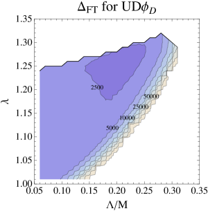
For a given value of the first three parameters, increasing simply increases the overall scale of the sparticle masses and -terms (while keeping the stop mixing fixed). Since increases monotonically with (by having heavier stops running in the loops), is uniquely determined by imposing GeV. This procedure can fail if some sparticles are tachyonic or if the basic conditions for electroweak symmetry breaking cannot be satisfied.
In almost all of the models which we discuss, either or does not talk to the messenger directly. That field will run tachyonic at high values of due to the leading terms in the soft masses being of the form,
| (3.5) |
where , are the contributions from the MSSM-messenger coupling and the standard GMSB contribution, respectively. So at a large enough value of , the squark becomes tachyonic. Solving for , this happens near,
| (3.6) |
This squark tachyon ceiling appears in nearly all models, although RG running from the messenger scale perturbs the actual value of (which manifests in gradual curves, as opposed to horizontal lines in space).
To explore each of these models, a dense grid of points in and is generated, with chosen to satisfy the GeV condition. We use SOFTSUSY Allanach:2001kg to run the spectra from the messenger scale to the TeV scale. As in CraigShih , contour plots in the plane completely characterize the viable parameter space of the model. If a particular point gives a valid solution, then the fine-tuning at that point is calculated using our tuning measure. As discussed in more detail in appendix B, the tuning measure is defined as
| (3.7) |
where with , , and measures the variation of the one-loop term (2.16). Each quantity is treated independently and varied separately.
The least tuned point located in each model is cataloged in table 1. The spectra of the models with low tuning will be discussed in detail in section 4. The type II model is the least tuned () out of all models, however, the rest of the type II models fare poorly with regards to tuning. In general, all of the type I squark models enter with a relatively low tuning measure of . Many of the models involving Higgs fields have very large (and small ) because they are relying on heavy stops to generate , as opposed to using maximal mixing. As these models are unable to achieve maximal mixing without substantial tuning entering elsewhere (due to the little problem), we make no effort to optimize the tuning in these models by scanning regions of parameter space where the MSSM-messenger contributions are small. Details concerning the various models will be discussed in the next subsections.
| # | Coupling | Best Point | Tuning | |||||
| I.1 | 1.98 | 3222 | 1842 | 777 | 3400 | |||
| I.2 | 1.99 | 3178 | 1828 | 789 | 2450 | |||
| I.3 | 4 | 2.05 | 2899 | 1709 | 668 | 3200 | ||
| I.4 | 4 | 0.58 | 11134 | 8993 | 2264 | 4050 | ||
| I.5 | 6 | 0.54 | 13290 | 9785 | 3408 | 3850 | ||
| I.6 | 6 | 0.67 | 11835 | 8637 | 3259 | 3410 | ||
| I.7 | 6 | 2.04 | 3020 | 1743 | 576 | 3500 | ||
| I.8 | 2.82 | 4336 | 1274 | 2056 | 1015 | |||
| I.9 | 2.67 | 4247 | 1342 | 2058 | 1015 | |||
| I.10 | 2.65 | 4040 | 1318 | 2301 | 1275 | |||
| I.11 | 2.76 | 4020 | 1257 | 2292 | 1260 | |||
| I.12 | 2.62 | 3815 | 1347 | 2070 | 1030 | |||
| I.13 | 2.91 | 3829 | 1199 | 2061 | 1020 | |||
| I.14 | 4 | 2.81 | 3575 | 1220 | 2312 | 1285 | ||
| I.15 | 4 | 2.63 | 3526 | 1312 | 2310 | 1280 | ||
| II.1 | 1 | 2.02 | 769 | 1965 | 2738 | 1800 | ||
| II.2 | 3 | 2.14 | 2203 | 1628 | 543 | 850 | ||
| II.3 | 3 | 2.27 | 2514 | 1458 | 439 | 1500 | ||
| II.4 | 1 | 1.78 | 2597 | 1829 | 3553 | 3020 | ||
| II.5 | 1 | 1.45 | 2497 | 2108 | 3773 | 6050 | ||
| II.6 | 1 | 0.22 | 7943 | 9870 | 3610 | 5000 | ||
| II.7 | 1 | 2.34 | 1374 | 1334 | 2998 | 2150 | ||
| II.8 | 1 | 1.51 | 1501 | 1204 | 2203 | 3700 | ||
| II.9 | 1 | 1.89 | 2004 | 1750 | 3373 | 2730 | ||
| II.10 | 5 | 2.13 | 2943 | 1649 | 282 | 3500 | ||
| II.11 | 0.54 | 7103 | 8166 | 3714 | 4930 | |||
| II.12 | 5 | 0.53 | 12629 | 9660 | 3333 | 3780 | ||
| II.13 | 5 | 0.65 | 11487 | 8710 | 3687 | 3380 | ||
| II.14 | 0.55 | 7049 | 8051 | 3255 | 5000 | |||
| II.15 | 5 | 0.57 | 12047 | 9213 | 1628 | 4220 | ||
| II.16 | 5 | 0.64 | 11571 | 8789 | 3665 | 3460 |
3.1 Type I Higgs couplings
We now survey the models in some detail, beginning with the type I Higgs models. As discussed in CraigShih , these models are all MFV, but they have high tuning because of the little problem.
With only a single MSSM-messenger coupling of the form appearing in the superpotential, the general form of the soft parameters from (2.20) can be easily specialized to the case of type I Higgs models:
| (3.8) |
where the multiplicity factors are defined , and is the sum of the quadratic Casimirs. The values in each model for , , and are displayed in table 2.
| # | Model | |||
|---|---|---|---|---|
| II.1 | ||||
| II.2 | ||||
| II.3 | ||||
| II.4 | ||||
| II.5 | ||||
| II.6 | ||||
| II.7 |
Qualitatively, all of the type I Higgs models have nearly congruent parameter spaces, with three common, characteristic features emerging, see fig. 2. These features were discussed at length in CraigShih ; let us briefly review them here. At lower , increasing gives a very large positive contribution to which quickly causes issues with EWSB. On the other hand, raising increases the negative contribution to from the one-loop term (2.16), which makes the viable region of larger. These two features combine to form the left, slanted edge of the viable regions shown in fig. 2. Increasing even further eventually caps by confronting it with a stop squark tachyon and drives even more negative (by raising the 1-loop term). As the model approaches , eventually the increasingly negative drives the sleptons tachyonic before the EWSB scale.
In different regions of the parameter space, the tuning parameter is dominated by different quantities. For low values of , the tuning is set by and . This is the case in all models, because as , the contributions from both and vanish and is generally subdominant. For moderate and small , is the biggest contributor to tuning. It is here that we find the lowest values of , and hence the lowest values of the tuning parameter. Finally, for larger , the contribution governs the tuning.
Finally, let us comment on some of the differences between type I Higgs models that are apparent from table 1.
-
•
The first two models – and – were studied in detail in CraigShih . For these models, different are possible. In type I Higgs models, increasing the messenger number within a specific model decreases the tuning for that model. This happens because and both scale as the number of messengers, thus , which makes it easier to achieve for a maximal contribution to the Higgs mass. For all the other type I Higgs models, only is possible because anything greater would violate the constraint.
-
•
Models I.4, I.5 and I.6 have small . These models forfeit maximal mixing in exchange for heavy stops. Models I.4 and I.5 are both identical to model I.1 in terms of their -terms and their contributions to soft masses, but in terms of their GMSB contribution to soft masses they have effective messenger number 4 and 6 respectively. As these models are unable to achieve maximal mixing without substantial tuning entering elsewhere, we do not optimize the tuning further by scanning into regions of parameter space where the MSSM-messenger contributions are vanishing.
-
•
Models I.3 and I.7 both have slightly better tuning than I.4-6. This is because these models receive an enhancement from the multiplicity factor . This enhancement provides larger -terms and allow significant stop mixing to be achieved.
3.2 Type I squark couplings
In the type I Higgs models, received a large correction , leading to the little problem and greater fine-tuning. Type I squark models receive an analogous correction to or , but this poses much less of a problem, as the electroweak symmetry breaking scale is only sensitive to the stop masses at loop level. Without the little problem, the type I squark models exhibit a significantly reduced tuning with respect to the type I Higgs models.
While the type I squark models fare well with regards to tuning, the lack of an MFV structure makes them more dangerous with regards to flavor constraints. These constraints can be evaded, however, if the EGMSB interactions are aligned with the third generation. Obviously, a sufficiently small perturbation around perfect alignment will continue to satisfy flavor constraints. Precisely how small this perturbation must be and whether this alignment can be achieved naturally are interesting questions for future studies paperwithArun . Regardless, while flavor appears alarming in these models, these concerns are insufficient to invalidate the models outright.
With only a single MSSM-messenger coupling of the form or appearing in the superpotential, the general form of the soft parameters can be derived from (2.20). For the type I -type models, we have,
| (3.9) |
and for the type I -type models, we have,
| (3.10) |
where as in the Higgs type models, we define the multiplicity factors and , or and as the sum of the quadratic Casimirs. The values of , , and in each model are shown in table 3.
| # | Model | |||
|---|---|---|---|---|
| II.8 | ||||
| II.9 | ||||
| II.10 | ||||
| II.11 |
| # | Model | |||
|---|---|---|---|---|
| II.12 | ||||
| II.13 | ||||
| II.14 | ||||
| II.15 |
As was the case in the type I Higgs models, increasing improves the tuning, however, here , due to one stop scaling as and the other as . The enhanced models, I.8-9 and I.12-13, possess slightly lower tuning than the models which cannot capitalize on this feature.
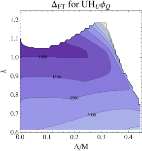
The parameter space of the type I squark models possesses a common, characteristic shape with two distinctive features – the “horn” and the “throat” – as shown in fig. 3. At high , the squark which does not interact with the messengers (either or ) is tachyonic, as discussed around (3.5). As decreases, the messenger scale increases, so the stops have more time to run negative, thus forbidding smaller values of and resulting in a curved viable region. Meanwhile, at intermediate and larger , the squark which does interact with the messengers can go tachyonic, as its soft mass is given schematically by,
| (3.11) |
where the are positive numbers, and the function is defined in (2.17). The combination of stop tachyons above and below in create a horn-like feature that extends into higher and . Going even lower in , eventually (3.11) will rise again, and the stop will cease to be tachyonic. This results in an excluded interval at intermediate , which we will call the “throat” region. It exists as long as is greater than some critical value:
| (3.12) |
where we have approximated .
At small , the tuning is set by and . The tuning in the interesting regions of these models is everywhere a balance of and , and at higher values of (i.e. on the horn region) the latter is leading. The region of lowest tuning in these models sits roughly on the underside of the base of the horn. This is sensible because one of the stops will run tachyonic near here, generating a larger . At the base, the tuning is set by . For two models (I.9 and I.13 – both shown in fig. 3), a second region of comparably good tuning sits in the middle of the horn. Although the stops are much heavier here, the tuning does not suffer greatly because the messenger scale has significantly decreased, and with it, has decreased resulting in a lower value of . Other type I squark models exhibit some regions of parameter space with a similarly decreasing , but the tuning is larger there.
We note that the least tuned type I squark models can achieve as low as , and we stress that all of these models have regions of parameter space that are significantly less tuned than all type I Higgs and nearly all type II models.
3.3 Type II couplings with mixing
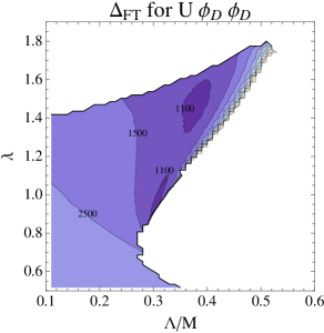
There are five type II (MSSM-MSSM-Messenger) couplings where the messenger mixes with one of the fields in an MSSM Yukawa coupling. Three of these couplings are top-Yukawa-like, , and , and two are bottom-Yukawa-like, and . The three top-Yukawa-like models are especially interesting because they provide an additional enhancement to by allowing two fields in to contribute to , (1.4). This enhancement is so effective that one of these models, , is the least tuned of all models, possessing regions with . Overall, all three of the mixed models are significantly less tuned than the other type II models, because of this enhancement.
In order to present the formulas for any type II model (with a coupling of the form ) in a general simplified form, we first define (similarly for , ). We can derive an expression from (2.23) which can be applied to each type II model – mixed or unmixed.333However, the can not be treated with these formulas due to the repeated . As this model is one of the most tuned models, we will not address it in detail. It is straightforward to derive the soft parameters in that model from (2.23). For these models, again with coupling , we have,
| (3.13) |
The piece of vanishes unless there is MSSM-messenger mixing, i.e. both and appear in the superpotential. The values are tabulated for each type II coupling in table 4. We now turn our focus to the individual models.
| # | Model | ||||
|---|---|---|---|---|---|
| III.1 | 1 | 2 | 3 | ||
| III.2 | 2 | 3 | 1 | ||
| III.3 | 1 | 3 | 2 | ||
| III.4 | 1 | 2 | 3 | ||
| III.5 | 1 | 3 | 2 | ||
| III.6 | 2 | 2 | 4 | ||
| III.7 | 2 | 2 | 2 | ||
| III.8 | 1 | 3 | 2 | ||
| III.9 | 1 | 3 | 1 | ||
| III.10 | 3 | 2 | 1 | ||
| III.11 | 1 | 1 | 2 | ||
| III.12 | 1 | 1 | 2 | ||
| III.13 | 1 | ||||
| III.14 | 1 | 1 | 2 | ||
| III.15 | 1 | 1 | 2 | ||
| III.16 | 1 |
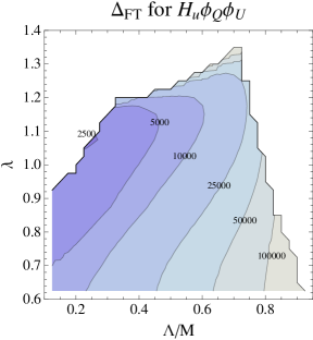
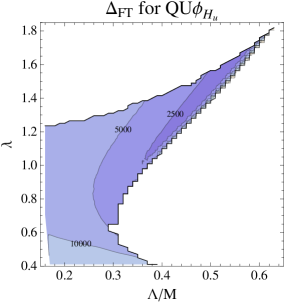
— This model is unique in that it is not bounded at high by any stop tachyons, although slepton tachyons provide a similar ceiling. Both stops receive a substantial enhancement to their soft masses from the mixing generated term. Unsurprisingly, this model occupies a parameter space with features very similar to many type I squark models. However, unlike those models, it is least tuned at high and high just above the region where is large enough to contribute negatively to the . The tuning in this model is controlled by and at high and low , respectively. The tuning in this model is shown in fig. 5.
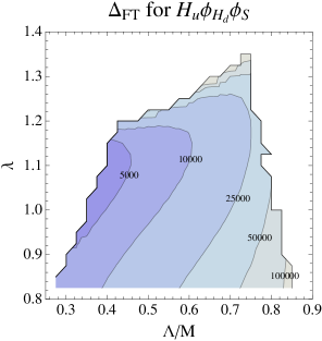
— Due to contributions from both and , this model receives the largest of any type II model, . Additionally, this is the least tuned of any model – type I or II. The tuning contours are shown in fig. 4. This model possesses many aspects of both the type I Higgs and squark models. is tachyonic at a relatively low , however, the and tachyons intersect near , so no horn feature appears in this model. As with the type I Higgs models, this model is least tuned for small because the one loop contribution to is large everywhere else. This leads a strip in near of lowest tuning. This strip is cut off from above by the large positive contribution to causing problems with EWSB (as in type I Higgs models), grows more tuned to the right from the increasingly negative and more tuned below by an increasing messenger scale. In the region of lowest tuning, is the largest contributor. For high and high , tuning is controlled by the one-loop contribution. At low , is the largest contributor to tuning.
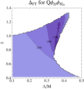
— This model, shown in fig. 4, is similar to , however the relation works against this model in two ways. First, the smaller multiplicity factor for means that the -term is not quite as large as in the model. Second, the larger multiplicity factor for gives a large contribution to from the mixing term and this contribution causes problems with EWSB at lower compared to the model. In particular, this cuts into the region where , further reducing the quality of this model. As in the model, the tuning at low is controlled by . At higher values, , and control the tuning for low, medium and high respectively.
— This model lives in a short slice of parameter space bounded by tachyons above and below by regions where EWSB cannot be achieved. The tuning in the model is controlled by everywhere. Since the mixing of this model gives additional enhancements proportional to , the effect of the mixing leads to only a minuscule contribution which makes no appreciable change to the case where the term is absent.
— This model lives in a rather narrow slice of parameter space bounded by tachyons above and tachyons below. The tuning in the model is governed everywhere by and . As the in the previous model which mixes with the bottom Yukawa, no significant change manifests from the effect of the mixing.
3.4 Type II couplings without mixing
The type II couplings without mixing, which frequently have very small viable regions in parameter space, tend to have high tuning. This is primarily because near a stop tachyon, is smaller (allowing for large ), but the viable regions in many type II models are sculpted in part by tachyons which are uncorrelated with . Additionally, these models do not receive any significant enhancement, as was the case for models II.1-II.3 as discussed in the previous subsection. We now briefly discuss the features of each model.
— Naively, one might expect this model to significantly enhance and manifest with regions of low tuning. However, it turns out that this model is prevented from ever achieving maximal mixing. First, since contributes doubly to , this results in a maximum MSSM-messenger coupling of before tachyons enter. Additionally, itself is tachyonic for all between . This is due to the same contributions which induce a squark throat (i.e. the discriminant in (3.12) is negative). Thus, this model has no valid solutions in any region with . The tuning in the small region that is valid in this model is governed by and , however, the MSSM-messenger coupling contribution is truly negligible here.
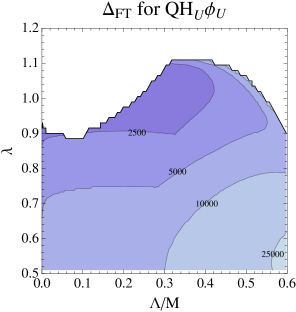
— This model, with tuning shown in fig. 5, lives in a small slice of parameter space bounded by tachyons above and tachyons below. The regions with the best tuning in this model are at higher values of near where is tachyonic. Encroaching on the region bounded below drives the SUSY breaking scale up rather drastically due to the growing so large that it provides a negative radiative correction to (this effect appears so pronounced in this model mostly due to the small parameter space considered). Near the very large regions, the tuning is set by , but in the regions of lower tuning, it is set by the term. Of all the unmixed type II models, this one presents with the lowest tuning.
— Perhaps unsurprisingly, this model is very similar to the model in the previous subsection. It lives in a short slice of parameter space bounded by tachyons above and by slepton tachyons below. Here, the tuning is controlled by and .
— This model is narrow in , but stretches further into than the other type II models before the tachyons above, and the tachyons below close the region. The tuning in the model is controlled by everywhere.
— This coupling involves , and a superfield with gauge charges like the bosons of Pati-Salam models. This model has similarities with both the Higgs and squark type I models. At low , raising causes issues with electroweak symmetry breaking. To the right a slight tachyon throat cuts off the model. The tuning is driven by , and .
— In addition to being horribly tuned, these models introduce a problem. Overall, the other features of these models is quite similar to the type I Higgs models. Note that for , the singlet field is insufficient to mediate SUSY breaking, so an additional with no superpotential interactions with the MSSM is assumed. The tuning is driven by and .
— These models have EWSB issues above and a slepton tachyon throat structure analogous to the squark throat discussed in section 3.2. However, more importantly these models introduce unacceptably large neutrino masses. Additionally, the singlet field is insufficient to mediate SUSY breaking, so an additional with no superpotential interactions with the MSSM is assumed. The tuning is driven by and .
4 Phenomenology
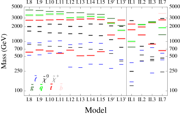
In this section, we discuss aspects of the phenomenology of the models that give . The models that satisfy this are: all type I squark models, the three mixed type II models – , and – and one other type II model – . Nearly all of these models possess spectra just beyond the reach of existing LHC searches. It is interesting to note that such heavy spectra actually seem to be a requirement of these GMSB models with a 125 GeV Higgs. This strongly suggests that the non-observation of SUSY and the presence of a heavy Higgs may be correlated issues rather than two distinct problems of SUSY.
4.1 Type I squark models
In the region of least tuning (the base of the horn in fig. 3), the type I squark models have heavy gluinos and first generation squarks falling between 3.5-5 and 3-4.5 TeV respectively, while the lightest stop (as well as the sbottom in models) has a mass between 0.5-1 TeV. Additionally, there is almost always an NLSP or co-NLSP s generally between 300-500 GeV (although these sometimes appear even heavier than GeV). However, the other region of low tuning appearing in models I.9 and I.13 (in the center of the horn) has a rather different profile (the best points of this second region are denoted by I.9′ and I.13′ in fig. 6). Here, the models have heavier stops, 1.2-2 TeV, but since has dropped significantly, the gluinos and first-generation squarks are now much lighter 2.0-3.5 TeV and 1.5-3 TeV, respectively. Surveying these points with less tuning, it is clear that the mass of the lightest stop and the masses of the gluino and first-generation squarks tend to be anti-correlated – thus, much of the parameter space with lower tuning possesses either squarks/gluinos or stops which can accessible at 14 TeV LHC.
Given a stop portal, there are three separate simplified topologies that arise:
-
1.
“NLSP” — with the stop appearing as either a co-NLSP with , or as the true NLSP (e.g. the best point of model I.11 in fig. 6)
-
2.
: : — Decays of
-
3.
: — This has competing decays of through an off-shell and
In all three cases, the NLSP decays to its SM partner plus gravitino. The first case is rare in these models, but has been discussed in the literature extensively, see e.g. Chou:1999zb ; Kats:2011it ; Han:2012fw ; Kaplan:2012gd ; Kilic:2012kw . The second case, which is slightly more common, will populate high , high multilepton searches – bounds for these will likely fall at or near the kinematic limit for production. The third case happens in models I.8-10,12-15 in fig. 6. The third case is most interesting in the limit where the top decay is squeezed out (). A sample spectrum which produces this signature is given by the best point of model I:14, as shown in fig. 6.
In this third case, when only the Higgsino-mediated decay can occur, the signature is two -jets with moderate , opposite sign s with very high and large additional . While in principle, several existing searches could have sensitivity to this exotic signature ATLAS:2012ht ; CMS-OS-DIL ; CMS-PAS-EXO-12-002 ; MT2:2012uu , those searches are not optimized to handle this kinematic configuration. Existing opposite sign searches tend to require a very hard jet and/or high . In the squeezed regime, the -jets will generally lack substantial enough to meet these strict cuts. Third generation leptoquark searches would have some sensitivity, however, the invariant mass and requirements may be too harsh for this specific signature since so much of the event’s energy is put into . Searches for in the system are likely the most sensitive probe of this system. Estimation based on the cuts in MT2:2012uu (as done for the similar signal examined in Evans:2012bf ) suggest this study repurposed would be sensitive to stops in the 450-550 GeV range. A dedicated search region either for s in the search or a hard region with softer cuts on the jets could likely probe significantly higher stop masses. Further exploration of this signature is an exciting subject for future work.
The distinct regions of low tuning appearing with heavier stops and lower (in models I.9 and I.13) can have accessible gluinos and first-generation squarks (these spectra are denoted I.9′ and I.13′ in fig. 6). These production portals result in complicated SUSY decay topologies with slepton co-NLSPs. These models will generically give hard jets, large , and multiple leptons. The 14 TeV extension of existing SUSY searches will be very sensitive to these topologies if the colored sparticles are light enough for a viable production cross-section. Regions in other type I squark models exhibit the same decreasing , but pay a substantial price in tuning. While the spectra are not shown, they manifest with the same qualitative features – rising stop masses with all other sparticles decreasing – which can allow for first-generation squark/gluino production.
4.2 Type II models
As one can easily infer from fig. 6, the type II models have more variation in their signatures. Generally these models possess lighter gluinos and first generation squarks. In fact, the points of best tuning in model II.1, the mixed model, are already ruled out by existing searches because these colored particles appear near or even below 1 TeV. However, in the other three less tuned models of type II, the gluinos are closer to 2 TeV and are not necessarily constrained by existing searches.
The least tuned type II model, II.2 (), has stops and bottoms near 1.5 TeV, but the other squarks and gluinos are near 2 TeV. For very low , these models will often have a NLSP, however, the bulk of parameter space does have a right-handed slepton co-NLSPs. In these low regions, the SUSY breaking scale can be high enough to for a detector stable neutralino. These models can present with classic SUSY signatures of multiple leptons, jets, and very high .
The colored states of model II.3, , are slightly heavy, with stops near 1 TeV and both first-generation squarks and gluinos appearing near 2.5 TeV. This spectra should be observable at 14 TeV LHC, where the production cross-section for 2.5 TeV gluinos and squarks is Beenakker:2011fu . However, even moving into regions with slightly higher masses, these models still have very light slepton co-NLSPs appearing near 200-300 GeV, which could be easily observed at a future ILC.
A slightly different topology, with stops, gluinos and first-generation squarks near 750 GeV, 1.5 TeV and 2 TeV, respectively manifests in model II.7, . Here, the Higgsino is very heavy, but the bino is always the NLSP. As above, these complicated topologies cannot be seen until 14 TeV, but give rise to classic SUSY signatures of multiple leptons, jets, and very high .
5 Conclusions
In this work, we studied models that produce large -terms through the introduction of a single marginal superpotential interaction between MSSM fields and the messengers of minimal GMSB. We classified all such interactions compatible with perturbative unification. Our complete list of 31 possible couplings – 15 type I couplings (MSSM-messenger-messenger) and 16 type II couplings (MSSM-MSSM-messenger) – is summarized in table 1.
Motivated by rampant confusion in the literature concerning the correct soft term contributions from MSSM-messenger interactions in the presence of MSSM-messenger mixing, we derived a new method for treating these interactions by directly integrating the wave functions in a manifestly holomorphic scheme. This conceptually straightforward method produced results applicable to all scenarios, whether or not fields are mixed. Formulas were presented for the soft parameters both in complete generality (2.15); and in the simpler special cases of only type I or type II couplings, (2.19)-(2.20) and (2.22)-(2.23) respectively.
Using these new formulas and a slight variation on the Barbieri-Giudice tuning measure, we surveyed the tuning in each of the 31 models. Under this examination, we concluded that the qualitatively similar type I Higgs models universally have high tuning due to the little problem, while the type I squark models can have tuning as low as . The majority of type II models have poor tuning, with the notable exception of the three models which allow for MSSM-messenger mixing with a top-Yukawa-like interaction, which generate a very large value for . The least tuned of these models, , manifests with the lowest tuning of any model studied in this work, , while the other two still have tuning below .
The spectra in the least tuned models usually have particles beyond the reach of the 8 TeV LHC, but can be accessible to the 14 TeV upgrade. This was not put in by hand, but is a consequence of the requirement that GeV, together with the minimal gauge mediated structure of the messenger sector. This suggests that the failure to find superpartners so far at the LHC was not an accident, but in fact had to be the case.
The models tend to possess either a stop below a TeV (and sometimes a sbottom as well) or accessible first-generation squarks and gluinos. The decay chain in these scenarios terminates with the light NLSP stau, co-NLSP sleptons or NLSP bino (with the rare exception of a stop NLSP) decaying to a gravitino. Both prompt and long-lived NLSP decays are possible in the models that we have considered. Production of the first-generation squarks and gluinos gives rise to classic SUSY signatures of high and with multiple leptons and hard jets. The scenarios with only stop production will usually given multi-lepton signatures; however, the cases with a stop NLSP or a squeezed transition are more difficult. The latter gives rise to a very interesting and poorly studied signature. Uncovering search strategies to improve sensitivity to this final state is an exciting avenue for future study. Another very common feature in these models is light sleptons (and occasionally Higginos) which could be readily produced and studied exhaustively at a TeV scale ILC.
While we took an agnostic approach to flavor physics in this work (assuming a perfect alignment), the lack of MFV in all of the least tuned models begs a thorough treatment of flavor. How much misalignment is permissible and whether alignment can be naturally achieved in a sensible way are both questions for future study. Another issue that we have not addressed in this paper is the origin of and . It would be very interesting to extend the models considered here to include a mechanism for . Perhaps extensions involving the NMSSM along the lines of CraigShih are viable. Finally, while we assumed single MSSM-messenger interaction terms for simplicity in this paper, it would be interesting to explore the effects of including of multiple MSSM-messenger interactions, as this could potentially generate regions of parameter space which exhibit even lower tuning.
Acknowledgments
We thank T. Jeliński, S. Knapen, A. Mariotti, Y. Shirman, A. Thalapillil, and B. Zhu for useful conversations. We thank B. Allanach for help with SOFTSUSY. JAE was supported by DOE grant DE-FG02-96ER40959. DS is supported in part by a DOE Early Career Award and a Sloan Foundation Fellowship.
Appendix A A Detailed Study of the Model
A.1 Applying our general formulas
In this appendix, we will provide an in-depth study of the model with
| (A.1) |
with . (We drop the 3rd generation subscript on and to avoid cluttering the equations.) In this model, the messenger has the same quantum numbers as . This is in many ways the prime example of a mixed type II model, given that it has been studied already in many papers Shadmi:2011hs ; Jelinski:2011xe ; Abdullah:2012tq ; Perez:2012mj ; Evans:2011bea ; Evans:2012hg ; Endo:2012rd . We will use this example to illustrate a number of points. First, it will highlight some interesting features of our general formulas. Second, by computing the soft masses in this model using other methods, it will provide a detailed check of our general formulas. Finally, we will use this example to illustrate the shortcomings of the formulas and approach in ChackoPonton which were mentioned in the body of the paper.
As seen in (2.23) and (3.13), the effect of MSSM-messenger mixing appears in the terms, so to focus on that, let us for simplicity set the gauge couplings and all other MSSM Yukawa couplings to zero. We begin by quoting the result of the general formula (3.13) for this model. Taking , , , and setting , we have:
| (A.2) |
with no contribution to other soft masses. Here, as in section 3, is shorthand for , etc. In the MSSM, we have , and , but it will be useful to leave these multiplicities general. Notice that the last two terms from (3.13) have cancelled out of and , leaving only the last line induced by the MSSM-messenger mixing. One can also check that by substituting the standard beta functions and anomalous dimensions into the formulas of ChackoPonton , one misses these extra terms. In the following subsections, we will study these extra terms in more detail. We will compute the soft mass-squareds in this model in two different ways: directly using SUSY correlators as in Craig:2013wga , and directly using wavefunction renormalization in the interaction basis. The latter will also illustrate the subtleties of wavefunction renormalization which the method derived in section 2 avoids.
A.2 Calculation using SUSY correlators
Let us calculate the directly, using a supersymmetric correlator formalism along the lines of Craig:2013wga . As in that paper, we separate out the -term-squared contribution to coming from integrating out the auxiliary field , and we will denote the remainder by the hatted quantity
| (A.3) |
This formulation is much simpler computationally, because it allows us to avoid various subtleties resulting from the treatment of contact terms and total derivatives.
The two-loop contribution to is given by
| (A.4) |
These correlators are evaluated in the Euclidean supersymmetric free theory and only contain 1PI diagrams with respect to the theory containing the auxiliary fields (in other words, if a diagram would become disconnected were an auxiliary field propagator removed, then it is not considered 1PI.) The subscripts are shorthand for the positions . In the second equation, we have rotated the supercharges so that they act on the operators at and , and then transformed this into of a simpler correlator. Comparing with (2.4), we can see that the correlator being differentiated is the 2-loop contribution to the wavefunction of . This is also clear diagrammatically, if we view this as the two-loop 1PI diagrams with external in the presence of the interactions (A.1).
It is straightforward to expand out all the terms in and perform the free-field contractions (keeping in mind the 1PI condition). The result is:
| (A.5) |
where
| (A.6) |
with shorthand for the integral over Euclidean phase space . It is easy to check that
| (A.7) |
We see that and contribute with equal magnitude and opposite sign to . Thus the contribution proportional to drops out, consistent with what we found in (A.2) using the general formula. However, the contribution from mixing proportional to remains. Combining (A.4), (A.5) and (A.7), and adding in , we find perfect agreement with (A.2).
Next, consider the soft mass for . This can be found by the same manipulations used to derive , but with . This agrees with the formula for in (A.2).
Finally, we come to . Here there is no -term-squared contribution, and we have:
| (A.8) |
which again agrees perfectly with (A.2).
A.3 Analytic continuation method
As another check of the general formulas, let us also perform the analytic continuation calculation by directly and explicitly integrating the wavefunctions, which can be easily done in this simple example. The trick is to do a unitary field redefinition to go to the interaction basis:
| (A.9) | |||||
| (A.10) |
So we will study the equivalent theory defined at the scale :
| (A.11) | |||
| (A.12) |
where
| (A.13) |
In the interaction basis, will receive wavefunction renormalization, but will not. This fact simplifies the calculation considerably.
Now we evolve this theory down to a lower scale. As in the previous subsections, we again neglect gauge couplings and the other Yukawas for simplicity. The result is:
| (A.14) |
where the wavefunctions obey the beta functions:
| (A.15) |
for . Here is the nonholomorphic Yukawa coupling in the theory with canonical Kähler potential. It obeys the beta function
| (A.16) |
with boundary condition . These equations can be integrated to obtain ; the result is
| (A.17) |
Next, at the scale , we integrate out the messengers supersymmetrically. This sets and . We additionally identify with below the messenger scale. At this theory then becomes
| (A.18) | |||
| (A.19) |
where . It is clear that the wavefunction of is discontinuous at the messenger scale. This is precisely the issue alluded to in section 2 arising from the mixing of and that prevents the formulas of ChackoPonton from being applied as presented.
Finally, we should proceed with wavefunction renormalization by again integrating (A.15)-(A.16), but now from to some lower scale . The key difference is that because of the discontinuity in the wavefunction, the boundary condition for the Yukawa coupling is also discontinuous:
| (A.20) |
Taking this into account, we find
| (A.21) |
Differentiating these expressions with respect to and and substituting (A.13) to recover the dependence on the original couplings, we again find perfect agreement with the general results (A.2) for .
Appendix B Fine-Tuning Measure
Fine-tuning is an inherently ambiguous concept. When comparing variations of two nearly identical parameters, it seems sensible, however even when comparing the variation of a mass parameter to a coupling the choice of measure quickly looks somewhat arbitrary. Since one of the objectives of this work is to determine which GMSB models possess lower fine-tuning, we demand that our fine-tuning measure, , satisfy certain properties:
-
1.
should provide a meaningful and accurate comparison between GMSB scenarios
-
2.
should never overlook contributions from large terms which cancel in a uncorrelated way
-
3.
should never introduce contributions from large terms which cancel in a correlated way
-
4.
should assign comparable sensitivity to two uncorrelated terms which cancel one another
Traditionally, the Barbieri-Guidice tuning measure GiudiceBarbieri is defined as:
| (B.1) |
where sums over a set of “fundamental” parameters. In general, it is not so clear what these fundamental parameters should be, and different choices for them lead to different numerical values of the tuning measure (the measure is not reparametrization invariant). For our purposes, we will adapt the Barbieri-Giudice tuning measure to be,
| (B.2) |
where and runs over all the important couplings in the theory, i.e. in this case, , although in practice only variations in , or manifest deviations large enough to matter quantitatively for this study. Thus, our set of parameters is . As in Feng:2012jfa , we choose to differentiate in (B.2) with respect to only parameters with mass squared units as this serves to better adhere to our requirement that canceling terms provide comparable sensitivities.
With the exception of (which is calculated directly), we compute these derivatives by implementing a very small fractional change in the parameters injected at the messenger scale, run down to the low scale and measure the change in using SOFTSUSY. , see (2.16), was chosen as the parameter to account for the dependence on (i.e. we fractionally vary the term rather than varying , , or some other combination of these parameters.). To keep variations in and orthogonal, we keep the 1-loop term fixed when we vary . This method removes the possibility for uncorrelated cancellations and correlated values being erroneously treated. Additionally, it is well defined in all of the GMSB scenarios we present here and, in principle, can be easily translated to work for many other GMSB scenarios as well.
References
- (1) ATLAS Collaboration Collaboration, G. Aad et al., Observation of a new particle in the search for the Standard Model Higgs boson with the ATLAS detector at the LHC, Phys.Lett. B716 (2012) 1–29, [arXiv:1207.7214].
- (2) CMS Collaboration Collaboration, S. Chatrchyan et al., Observation of a new boson at a mass of 125 GeV with the CMS experiment at the LHC, Phys.Lett. B716 (2012) 30–61, [arXiv:1207.7235].
- (3) L. J. Hall, D. Pinner, and J. T. Ruderman, A Natural SUSY Higgs Near 126 GeV, JHEP 1204 (2012) 131, [arXiv:1112.2703].
- (4) S. Heinemeyer, O. Stal, and G. Weiglein, Interpreting the LHC Higgs Search Results in the MSSM, Phys.Lett. B710 (2012) 201–206, [arXiv:1112.3026].
- (5) A. Arbey, M. Battaglia, A. Djouadi, F. Mahmoudi, and J. Quevillon, Implications of a 125 GeV Higgs for supersymmetric models, Phys.Lett. B708 (2012) 162–169, [arXiv:1112.3028].
- (6) P. Draper, P. Meade, M. Reece, and D. Shih, Implications of a 125 GeV Higgs for the MSSM and Low-Scale SUSY Breaking, Phys.Rev. D85 (2012) 095007, [arXiv:1112.3068].
- (7) M. Carena, S. Gori, N. R. Shah, and C. E. Wagner, A 125 GeV SM-like Higgs in the MSSM and the rate, JHEP 1203 (2012) 014, [arXiv:1112.3336].
- (8) J. Casas, J. Espinosa, M. Quiros, and A. Riotto, The Lightest Higgs boson mass in the minimal supersymmetric standard model, Nucl.Phys. B436 (1995) 3–29, [hep-ph/9407389].
- (9) M. S. Carena, J. Espinosa, M. Quiros, and C. Wagner, Analytical expressions for radiatively corrected Higgs masses and couplings in the MSSM, Phys.Lett. B355 (1995) 209–221, [hep-ph/9504316].
- (10) H. E. Haber, R. Hempfling, and A. H. Hoang, Approximating the radiatively corrected Higgs mass in the minimal supersymmetric model, Z.Phys. C75 (1997) 539–554, [hep-ph/9609331].
- (11) G. Giudice and R. Rattazzi, Theories with gauge mediated supersymmetry breaking, Phys.Rept. 322 (1999) 419–499, [hep-ph/9801271].
- (12) M. A. Ajaib, I. Gogoladze, F. Nasir, and Q. Shafi, Revisiting mGMSB in light of a 125 GeV Higgs, arXiv:1204.2856.
- (13) Z. Chacko and E. Ponton, Yukawa deflected gauge mediation, Phys.Rev. D66 (2002) 095004, [hep-ph/0112190].
- (14) Y. Shadmi and P. Z. Szabo, Flavored Gauge-Mediation, JHEP 1206 (2012) 124, [arXiv:1103.0292].
- (15) J. L. Evans, M. Ibe, and T. T. Yanagida, Relatively Heavy Higgs Boson in More Generic Gauge Mediation, Phys.Lett. B705 (2011) 342–348, [arXiv:1107.3006].
- (16) T. Jelinski, J. Pawelczyk, and K. Turzynski, On Low-Energy Predictions of Unification Models Inspired by F-theory, Phys.Lett. B711 (2012) 307–312, [arXiv:1111.6492].
- (17) J. L. Evans, M. Ibe, S. Shirai, and T. T. Yanagida, A 125GeV Higgs Boson and Muon g-2 in More Generic Gauge Mediation, Phys.Rev. D85 (2012) 095004, [arXiv:1201.2611].
- (18) A. Albaid and K. Babu, Higgs boson of mass 125 GeV in GMSB models with messenger-matter mixing, arXiv:1207.1014.
- (19) M. Abdullah, I. Galon, Y. Shadmi, and Y. Shirman, Flavored Gauge Mediation, A Heavy Higgs, and Supersymmetric Alignment, arXiv:1209.4904.
- (20) M. J. Perez, P. Ramond, and J. Zhang, On Mixing Supersymmetry and Family Symmetry Breakings, arXiv:1209.6071.
- (21) M. Endo, K. Hamaguchi, S. Iwamoto, and N. Yokozaki, Vacuum Stability Bound on Extended GMSB Models, JHEP 1206 (2012) 060, [arXiv:1202.2751].
- (22) N. Craig, S. Knapen, D. Shih, and Y. Zhao, A Complete Model of Low-Scale Gauge Mediation, arXiv:1206.4086.
- (23) N. Craig, S. Knapen, and D. Shih, General Messenger Higgs Mediation, arXiv:1302.2642.
- (24) G. F. Giudice, H. D. Kim, and R. Rattazzi, Natural mu and B mu in gauge mediation, Phys.Lett. B660 (2008) 545–549, [arXiv:0711.4448].
- (25) G. Giudice and R. Rattazzi, Extracting supersymmetry breaking effects from wave function renormalization, Nucl.Phys. B511 (1998) 25–44, [hep-ph/9706540].
- (26) S. P. Martin and M. T. Vaughn, Two loop renormalization group equations for soft supersymmetry breaking couplings, Phys.Rev. D50 (1994) 2282, [hep-ph/9311340].
- (27) R. Barbieri and G. Giudice, Upper Bounds on Supersymmetric Particle Masses, Nucl.Phys. B306 (1988) 63.
- (28) Z. Kang, T. Li, T. Liu, C. Tong, and J. M. Yang, A Heavy SM-like Higgs and a Light Stop from Yukawa-Deflected Gauge Mediation, Phys.Rev. D86 (2012) 095020, [arXiv:1203.2336].
- (29) J. A. Evans, D. Shih, and A. Thalapillil. To appear.
- (30) H. D. Kim, Electroweak symmetry breaking from SUSY breaking with bosonic see-saw mechanism, Phys.Rev. D72 (2005) 055015, [hep-ph/0501059].
- (31) F. Joaquim and A. Rossi, Phenomenology of the triplet seesaw mechanism with Gauge and Yukawa mediation of SUSY breaking, Nucl.Phys. B765 (2007) 71–117, [hep-ph/0607298].
- (32) H. D. Kim, D. Y. Mo, and M.-S. Seo, Neutrino Assisted Gauge Mediation, arXiv:1211.6479.
- (33) P. Byakti and T. S. Ray, Burgeoning the Higgs mass to 125 GeV through messenger-matter interactions in GMSB models, arXiv:1301.7605.
- (34) B. Allanach, SOFTSUSY: a program for calculating supersymmetric spectra, Comput.Phys.Commun. 143 (2002) 305–331, [hep-ph/0104145].
- (35) C.-L. Chou and M. E. Peskin, Scalar top quark as the next-to-lightest supersymmetric particle, Phys.Rev. D61 (2000) 055004, [hep-ph/9909536].
- (36) Y. Kats and D. Shih, Light Stop NLSPs at the Tevatron and LHC, JHEP 1108 (2011) 049, [arXiv:1106.0030].
- (37) Z. Han, A. Katz, D. Krohn, and M. Reece, (Light) Stop Signs, JHEP 1208 (2012) 083, [arXiv:1205.5808].
- (38) D. E. Kaplan, K. Rehermann, and D. Stolarski, Searching for Direct Stop Production in Hadronic Top Data at the LHC, JHEP 1207 (2012) 119, [arXiv:1205.5816].
- (39) C. Kilic and B. Tweedie, Cornering Light Stops with Dileptonic mT2, arXiv:1211.6106.
- (40) ATLAS Collaboration Collaboration, G. Aad et al., Search for Supersymmetry in Events with Large Missing Transverse Momentum, Jets, and at Least One Tau Lepton in 7 TeV Proton-Proton Collision Data with the ATLAS Detector, Eur.Phys.J. C72 (2012) 2215, [arXiv:1210.1314].
- (41) CMS Collaboration, Search for new physics in events with opposite-sign leptons, jets, and missing transverse energy in collisions at TeV, Phys.Lett. B718 (2013) 815, [arXiv:1206.3949].
- (42) CMS Collaboration, Search for pair production of third-generation leptoquarks and top squarks in collisions at TeV, arXiv:1210.5629.
- (43) ATLAS Collaboration, Search for a heavy top-quark partner in final states with two leptons with the ATLAS detector at the LHC, JHEP 1211 (2012) 094, [arXiv:1209.4186].
- (44) J. A. Evans and Y. Kats, LHC Coverage of RPV MSSM with Light Stops, arXiv:1209.0764.
- (45) W. Beenakker, S. Brensing, M. Kramer, A. Kulesza, E. Laenen, et al., Squark and Gluino Hadroproduction, Int.J.Mod.Phys. A26 (2011) 2637–2664, [arXiv:1105.1110].
- (46) J. L. Feng and D. Sanford, A Natural 125 GeV Higgs Boson in the MSSM from Focus Point Supersymmetry with A-Terms, Phys.Rev. D86 (2012) 055015, [arXiv:1205.2372].