Quantum Stabilization of a Closed Nielsen–Olesen String

Abstract

We revisit the classical instability of closed strings in the Abelian Higgs model. The instability is expressed by a vanishing energy as the torus-like configuration shrinks to zero size. We treat the radius of the torus as a collective coordinate and demonstrate that a quantum mechanical treatment of this coordinate leads to a stabilization of the closed string at small radii.

I Introduction and Motivation

The study of string or vortex type configurations in the Standard Model and related theories has attracted much attention in the recent past Hindmarsh:1994re ; Kibble:1976sj ; Vilenkin:1994 ; Achucarro:2008fn ; Copeland:2009ga . Because these configurations may have cosmological implications and to distinguish them from the fundamental objects in string theory, they are commonly called cosmic strings. The most imperative question regarding the dynamics of a cosmic string is its stability. Studies of this question have mainly focused on infinitely long and axially symmetric string configurations Nielsen:1973cs ; Nambu:1977ag ; Vachaspati:1992fi ; Naculich:1995cb ; Achucarro:1999it ; Groves:1999ks ; Stojkovic ; Bordag:2003at ; Graham:2004jb ; Graham:2006qt ; Schroder:2007xk ; Baacke:2008sq ; Weigel:2009wi ; Weigel:2010pf ; Lilley:2010av ; Weigel:2010zk ; Graham:2011fw . Unless these configurations carry (topological) charges, as is the case, for example, for the Abelian Nielsen-Olesen string Nielsen:1973cs , they are classically unstable but can eventually be stabilized by quantum effects. One such possibility would be to bind (a large number of) fermions at the center of the string Weigel:2010zk ; Graham:2011fw . Other stabilizing mechanisms involve the coupling of external fields or currents leading to superconducting strings Witten:1984eb .

Strings at the boundary of regions with different vacuum expectation values are expected to build a network, so that they have the potential to form cosmic string loops Witten:1984eb ; Davis:1988ij . As a consequence, it is conceivable that closed strings or a network thereof existed at early times of the universe when the vacuum manifold was not simply connected. Cosmologically motivated studies on networks of closed strings suggested their stability (against graviational radiation) for radii of the order of a a small fraction $\sim\mathscr{O}(0.01\ldots 0.1)$ of the horizon distance. These studies started from analytic investigations Vilenkin:1981iu ; Kibble:1982cb ; Burden:1985md but were followed by intensive numerical simulations, cf. the recent article BlancoPillado:2011dq for a comprehensive discussion of these activities over the past two decades.

Eventually such closed strings would relax to circular (torus-like) configurations, so-called vortons Davis:1988ij . Typically such vortons are stabilized by coupling to (external) currents Witten:1984eb ; Davis:1988ip ; Davis:1988jq ; Davis:1995kk ; Davis:1996xs ; Davis:1999ec . The existence of vortons in a super–conducting scenario was supported by numerical studies some time ago Lemperiere:2002en .

It is also interesting, however, to see whether such closed strings are self-stabilizing in the sense that the dynamics of the underlying Lagrangian prevents them from contracting and eventually disappearing. We are particularly interested in quantum self-interactions of a single closed string. We expect that these quantum effects become significant for strings with radii similar to the Compton wave-lengths of the fields within the Lagrangian. In such a scenario the string would lose energy by emitting fluctuations of its own field rather than by graviational radiation.

Closed strings are not subject to any non-trivial boundary condition at spatial infinity and are therefore not stabilized topologically. On the contrary, simple dimensional arguments show that closed strings can reduce their energy by shrinking. Hence they are not stabilized dynamically either, at least on the classical level. The naïve conclusion would be that even if a closed string had existed at some earlier time it would have decayed by emitting radiation and simultaneously shrinking to zero size. However, this argumentation cannot be correct at the quantum level because narrow configurations localize the particle in position space which, by the uncertainty principle, implies that large momenta emerge and prevent the total energy from vanishing.

We will consider this question for the flux tube in scalar electrodynamics and study the analog of the Nielsen-Olesen string on a torus of radius $R$. In this case a classical instability occurs as $R\to 0$. The study of a toroidal string configuration is significantly more complicated than that of an infinitely long and axially symmetric string because the field equations cannot be simplified to ordinary differential equations of a single variable. This hampers the application of spectral methods, which have previously been used successfully to compute quantum effects for localized field configurations Graham:2009zz . We will therefore adopt a different technique that has proven successful in describing similar quantum mechanical scenarios. It is based on the quantum mechanical uncertainty relation

$$\Delta p\Delta x\geq\frac{\hbar}{2}$$ (1)

and assumes that for the ground state the momentum $p$ is saturated by $\Delta p$ and that $\Delta x$ is a good approximation for the spatial extension, $x$. Minimizing the Hamiltonian that is constructed from the replacement $p\longrightarrow\nicefrac{{\hbar}}{{(2x)}}$ yields the correct ground state energy and extension for both the hydrogen atom (which is also classically unstable) and the harmonic oscillator.

In order to apply this approach, the appropriate momentum (operator) must be identified. We will do this by introducing a time-dependent collective coordinate for the extension of the field configuration in which the classical instability occurs. The conjugate momentum is then extracted from the Lagrangian and the system is quantized by imposing the canonical commutation relation between the collective coordinate and its conjugate momentum. This so-called collective coordinate quantization reasonably reproduces quantum properties of localized field configurations in various examples Weigel:2008zz . Rather than exploring the full quantum theory, this formulation concentrates on the physically important modes. In the case of a collapsing cosmic string, the most relevant mode is obviously the radius $R$ of the torus on which the string lives.

The paper is organized as follows. First, we complete this introduction by describing the model of scalar electrodynamics that we use. In section II we briefly review the Nielsen-Olesen string in the axially symmetric framework. In section III we provide a detailed description of toroidal coordinates and explain the string configuration that respects this symmetry. In particular, we derive consistent boundary conditions. As expected from dimensional considerations, we find that the classical toroidal string is unstable against shrinking to zero size. We therefore introduce a collective coordinate for this mode, which we quantize canonically (section IV). We estimate the corresponding contribution to the energy from Heisenberg’s uncertainty principle and derive a quantum energy functional whose minimum we seek. Since the system cannot be decomposed into one-dimensional problems, the numerical investigations are challenging. We relegate their description to appendices. Section V summarizes and concludes our studies.

We consider scalar electrodynamics with the Lagrangian

$$\mathscr{L}=-\frac{1}{4}\,F_{\mu\nu}\,F^{\mu\nu}+\big{|}D_{\mu}\,\Phi\big{|}^{2}-V(\Phi)\,,$$ (2)

where the covariant derivative and scalar potential are

$$D_{\mu}=\partial_{\mu}+ieA_{\mu}\qquad{\rm and}\qquad V(\Phi)=m^{2}\,|\Phi|^{2}+\lambda\,|\Phi|^{4}\,,$$ (3)

respectively. To induce spontaneous symmetry breaking, we take $m^{2}<0$ and observe the classical vacuum expectation value (vev)

$$\big{\langle}|\Phi|\big{\rangle}=\sqrt{\frac{-m^{2}}{2\lambda}}\equiv v\,.$$ (4)

Notice that $\Phi$ and $v$ have dimension of mass in $(3+1)$ dimensions, while $\lambda$ and $e$ are dimensionless. The (tree-level) masses of the Higgs and gauge fields can be identified by considering fluctuations about the $vev$ in the Lagrangian in eq. (2),

$$m_{\Phi}^{2}=4\lambda v^{2}\,,\qquad\qquad m_{A}^{2}=2e^{2}v^{2}\,.$$ (5)

For later reference, we briefly discuss the equation of motion for the temporal component of the gauge field (Gauß’ law),

$$\big{(}-\Delta+2e^{2}|\Phi|^{2}\big{)}\,A_{0}=ie\,(\Phi^{\ast}\partial_{0}\Phi-\Phi\partial_{0}\Phi^{\ast})+\nabla\cdot\dot{\mathbf{A}}\,,$$ (6)

where the dot denotes a time derivative. Clearly, this equation contains no time derivative for ${A}_{0}$, and is therefore a constraint on $A_{0}$ rather than a true dynamical equation. Furthermore, it is an elliptic differential equation and as such has the unique solution $A_{0}=0$ (given proper boundary conditions at spatial infinity) if the right hand side of eq. (6) vanishes. This happens if (i) the phase of the Higgs field is time-independent and (ii) the gauge field $\mathbf{A}$ is either time-independent ($\dot{\mathbf{A}}=0$) or transverse ($\nabla\cdot\mathbf{A}=0$). It is, of course, possible to enforce the transversality of $\mathbf{A}$ (or the Weyl condition $A_{0}=0$) by a choice of gauge, even for time-dependent fields. The respective gauge transformations will, however, be time-dependent and highly non-local, leading to very cumbersome contributions to the phase of the Higgs field and the kinetic energy of both $\mathbf{A}$ and $\Phi$. Since the kinetic energy is essential for the potential quantum stabilization of a closed string (cf. section IV), it is very inconvenient to enforce the Coulomb or Weyl condition in order to resolve Gauß’ law. Instead, we have to implement eq. (6) and allow for $A_{0}\neq 0$ when introducing the time-dependent field configurations necessary for a quantum mechanical treatment.

II Infinitely long Nielsen–Olesen string

Before discussing our toroidal string configuration in more detail, let us briefly review the well-known Nielsen–Olesen (NO) string Nielsen:1973cs which corresponds to the limit that the (outer) torus radius becomes infinitely large. This string is a static, infinitely long vortex configuration stretched along the $z$-axis, in which the Higgs field $\Phi$ has winding number $n$, and the magnetic field points along the string axis, $\mathbf{B}\sim\mathbf{e}_{z}$:

$$\mathbf{A}=g(r)\,\frac{n}{er}\,\mathbf{e}_{\varphi}\,,\qquad\qquad\Phi=v\,f(r)\,e^{+in\varphi}\,.$$ (7)

(We are using polar coordinates $(r,\varphi)$ in the $xy$-plane). Notice that $\nabla\times\mathbf{A}=0$ and $A_{0}=0$ for this ansatz, which is consistent with Gauß’ law because the Higgs field $\Phi$ is time-independent. The requirements of finite energy and continuity at the origin then lead to boundary conditions on the profile functions $f$ and $g$,

$$\begin{array}[]{rclcl}r\to 0&:&f(r)\to 0\,,&&g(r)\to 0\\[5.69054pt] r\to\infty&:&f(r)\to 1\,,&&g(r)\to 1\end{array}$$ (8)

The NO string owes its stability to the fact that the Higgs field at spatial infinity defines a map $S^{1}\mapsto U(1)$, which in view of $\pi_{1}(U(1))=\mathbbm{Z}$ cannot be continuously deformed into the vacuum.

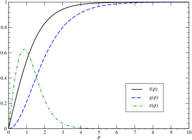
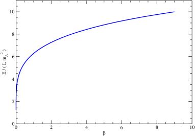
Figure 1: (Color online) Left panel: Nielsen–Oleson profiles for the infinitely long straight string for the mass ratio $\beta=1$. Also shown is the energy density, i.e. the integrand of eq. (10). Right panel: The energy per unit length, eq. (10), as a function of $\beta$ at fixed $e^{2}=\frac{1}{2}$.

We note that our model, as given by eq. (2), initially has three parameters, the Higgs vev $v$ and the two coupling constants $\lambda$ and $e$ (or, equivalently, the two masses in eq. (5)). After rescaling all dimensionful quantities in units of some appropriate scale, we expect all observables to be functions of the two couplings $\lambda$ and $e$ independently. However, this is not always true: In the NO string, for instance, the profile functions only depend on the ratio

$$\beta=\frac{m_{\Phi}^{2}}{m_{A}^{2}}=\frac{2\lambda}{e^{2}}$$ (9)

once the fundamental scale is chosen as the mass of the gauge field, $m_{A}$ (and the winding number is fixed to $n=1$). This is because the gauge coupling $e$ scales out in an overall prefactor for the (dimensionless) energy per unit length,

$$\frac{E}{m_{A}^{2}\,L}=\frac{\pi}{e^{2}}\int\limits_{0}^{\infty}d\rho\,\rho\,\left\{\frac{n^{2}}{\rho^{2}}\,g^{\prime}(\rho)^{2}+\Big{[}f^{\prime}(\rho)^{2}+\frac{n^{2}}{\rho^{2}}\,f(\rho)^{2}\,\left(1-g(\rho)\right)^{2}\Big{]}+\frac{\beta}{4}\,(1-f(\rho)^{2})^{2}\right\}\,,$$ (10)

where $\rho\equiv m_{A}\,r$ is the scaled distance from the symmetry axis. The NO profiles $f(\rho)$ and $g(\rho)$ resulting from the minimization of this functional will only depend on the ratio $\beta$, because any change of couplings that leaves $\beta$ invariant can at most produce an overall prefactor to the functional (10), which is irrelevant for the minimization. The value of the (minimal) energy per unit length will then scale trivially with $e$ at fixed $\beta$. In figure 1, we present the numerical solutions for the NO profiles in the case $\beta=1$, and the value of the minimal energy per unit length as a function of $\beta$ at fixed $e^{2}=1/2$. For our preferred values

$$e^{2}=\frac{1}{2}\,,\quad\lambda=\frac{1}{4}\qquad\Longrightarrow\qquad m_{A}=m_{\Phi}=v\quad\mbox{and}\quad\beta=1\,,$$ (11)

we find a minimal energy per unit length of $6.28\,m_{A}^{2}$; this will provide an important numerical check for the torus configuration discussed in the next section.

III Toroidal coordinates and strings

We construct a closed string from the NO configuration by first assuming that the latter has a finite (though very large) length $L=2\pi R$ and then identifying its two end surfaces. The core of the string, along which the profile functions $f$ and $g$ vanish, thus becomes a circle of radius $R$. Moreover, the radial coordinate $\rho$, i.e. the independent variable of the NO string, then measures the distance from this circle, and surfaces of constant $\rho\neq 0$ are tori. We will be particularly interested in the change of the profile functions as the core radius $R$ decreases and becomes as small as the Compton wave-lengths of the particles in the model. Eventually $R$ will be considered a variational parameter which will be determined by minimizing the (quantum) energy of the torus configuration.

The NO string is characterized by a rotational symmetry about its core. This cannot be maintained once the string is closed, because the direction in which one moves away from the core does matter: If one moves away in the direction of spatial infinity, the fields have an infinite range to decay to their vacuum values, while there is only a finite distance when moving towards the center of the core circle. (And it is even not necessarily true that the fields assume their vacuum values at the center.) As a consequence, the lines of constant energy density must be denser on the inside of the core than on its outside, and since these situations are related by rotations about the core axis, there cannot be any axial symmetry. While the profile functions at spatial infinity are still subject to boundary conditions, they will result from the dynamics at the center of the circle. The loss of axial symmetry causes the profile functions to depend on more than one coordinate, which complicates matters significantly. The only remaining symmetry is that along the core circle.

III.1 Geometry of the torus configuration

The previous considerations strongly suggest the introduction of toroidal coordinates which we describe in this subsection. We choose to put the circle of the string’s core in the $xy$-plane of a Cartesian coordinate system and center it at the origin. The corresponding toroidal coordinates read book_MF :

$$x =R\,\frac{\sinh\tau}{\cosh\tau-\cos\sigma}\,\cos\varphi$$

$$y =R\,\frac{\sinh\tau}{\cosh\tau-\cos\sigma}\,\sin\varphi$$

$$z =R\,\frac{\sin\sigma}{\cosh\tau-\cos\sigma}\,.$$ (12)

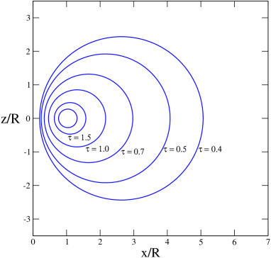
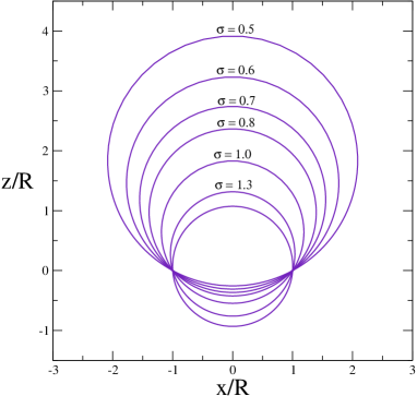
Figure 2: (Color online) Coordinate lines of toroidal coordinates in the $xy$-plane ($\varphi=0$ and $\varphi=\pi$). Left panel: Lines of constant $\tau$ (at $\varphi=0$ only, $\varphi=\pi$ is the mirror image about the $z$-axis). Right panel: Lines of constant $\sigma$. Each circle is composed of two distinct coordinate lines, namely $\sigma\in[0,\pi/2]$ (above the foci) and $(\sigma+\pi)$ (below the foci). The remaining $\sigma$ range gives mirror images which are not displayed for simplicity.

The coordinate $\varphi\in[0,2\pi]$ is the usual polar angle describing the rotation of the $xz$-plane around the vertical $z$-axis. By construction, this rotation is a symmetry of our configuration and $\varphi$ is a cyclic coordinate that describes the position along the string core. The coordinate $\tau\in[0,\infty]$ is best understood from its iso-lines in the left panel of fig. 2. Smaller values of $\tau$ correspond to larger circles that spread out towards infinity on the outside, and approach the vertical axis on the inside, while the center of these circles gradually moves away from the torus core. The inverse $\tau^{-1}$ is therefore (highly non-linearly) related to the distance from the string core (similarly to the radius $\rho$ in the NO string), although it cannot be directly identified with this quantity. Finally, the angle $\sigma\in[0,2\pi]$ describes the different points on the $\tau$-coordinate lines. When viewed from the core, it plays the role of an azimuthal angle. It is therefore natural to give the Higgs field winding by taking $\sigma$ as its phase. Then the profiles are predominantly functions of $\tau$ only, with a $\sigma$-modulation mainly in the vicinity of the origin. Note that origin of the coordinate system corresponds to $\tau=0$ and $\sigma=\pi$ while spatial infinity is approached as $\tau\to 0$ and $\sigma\to 0$.

The above considerations lead to the following ansatz for the closed string field configuration Postma:2007bf

$$\Phi=v\,f(\sigma,\tau)\,e^{in\sigma}\,,\qquad\qquad\mathbf{A}=A(\sigma,\tau)\,\mathbf{e}_{\sigma}\,,$$ (13)

where $\mathbf{e}_{\sigma}$ is the tangential unit vector along the lines in the left panel of figure 2. To ensure finite energy, we must have $|\mathbf{D}\Phi|\to 0$ at large distances, which implies

$$A(\sigma,\tau)\to\frac{n}{e}\,\frac{1}{h(\sigma,\tau)}=\frac{n}{e}\,\frac{\cosh\tau-\cos\sigma}{R}\,.$$ (14)

Here, the gradient in toroidal coordinates gives rise to the metric factor

$$h(\sigma,\tau)\equiv\frac{R}{\cosh\tau-\cos\sigma}\,.$$ (15)

In view of these asymptotics, we refine our ansatz to the form

$$\Phi(\mathbf{x})=vf(\sigma,\tau)\,e^{in\sigma}\,,\qquad\qquad\mathbf{A}(\mathbf{x})=\frac{n}{e}\,\frac{g(\sigma,\tau)}{h(\sigma,\tau)}\,\mathbf{e}_{\sigma}\,,$$ (16)

with suitable boundary conditions on the profiles discussed below. Since the configuration eq. (16) is time-independent, we can discard any temporal gauge field component and put $A_{0}=0$ to resolve Gauß’ law. Note, however, that the gauge field is no longer transverse,

$$\nabla\cdot\mathbf{A}=\frac{n}{e}\,\frac{1}{h(\sigma,\tau)^{3}}\,\frac{\partial}{\partial\sigma}\,\Big{[}g(\sigma,\tau)\,h(\sigma,\tau)\Big{]}\neq 0\,.$$ (17)

As expected, the magnetic field

$$\mathbf{B}=\nabla\times\mathbf{A}=-\frac{n}{e}\frac{\partial_{\tau}g(\sigma,\tau)}{h(\sigma,\tau)}\,\mathbf{e}_{\varphi}$$ (18)

of the closed string points in $\mathbf{e}_{\varphi}$-direction, i.e. along the core of the string.

III.2 Classical energy and boundary conditions

Since our closed string ansatz is static, its energy density is just minus its Lagrangian density. The classical energy becomes, upon integration over space,

$$\frac{E}{m_{A}}=\frac{\pi}{e^{2}}\int_{0}^{\infty}d\tau\int_{-\pi}^{\pi}d\sigma\,\sinh\tau\,\Bigg{\{}\frac{n^{2}}{\hat{R}\eta}\, (\partial_{\tau}g)^{2}+\hat{R}\eta\,\Big{[}(\partial_{\tau}f)^{2}+n^{2}f^{2}\,\big{(}1-g\big{)}^{2}+(\partial_{\sigma}f)^{2}\Big{]}+$$

$$+\frac{\beta}{4}\,\hat{R}^{3}\,\eta^{3}\,\big{(}1-f^{2}\big{)}^{2}\Bigg{\}}\,.$$ (19)

As in the case of the NO string we have scaled all dimensionful quantities by appropriate powers of the mass of the gauge boson, $m_{A}$:

$$\hat{R}\equiv m_{A}\,R\,,\qquad\qquad\eta(\sigma,\tau)\equiv\frac{h(\sigma,\tau)}{R}=\frac{1}{\cosh\tau-\cos\sigma}\,.$$ (20)

Again, the gauge coupling $e$ only appears as an overall prefactor, and the profiles only depend on the mass ratio $\beta$. In addition we observe a non-trivial dependence on the radius $R$.

To complete the discussion of the classical torus configuration, we need to specify the boundary conditions for the profile functions $f$ and $g$. Since $\sigma$ is an angle variable and the profiles have to be single-valued, it is immediately clear that we must impose periodic boundary conditions in $\sigma$-direction,

$$f(0,\tau)=f(2\pi,\tau)\,,\qquad\qquad g(0,\tau)=g(2\pi,\tau)\,.$$ (21)

At $\tau\to\infty$, we are on the core circle where we expect the initial $U(1)$ symmetry to be restored, i.e. the Higgs vev vanishes. To avoid singularities at $\tau\to\infty$, the magnetic field and even the gauge potential itself must also vanish on the core line. This enforces Dirichlet conditions

$$f(\sigma,\infty)=g(\sigma,\infty)=0\,.$$ (22)

Finally, we have to find the conditions for the limit $\tau\to 0$. This corresponds to the largest circles in the left panel of fig. 2 and includes spatial infinity ($\sigma\to 0,2\pi$) and the vertical $z$-axis ($\sigma\neq 0,2\pi$). The first case obviously requires the vacuum configuration $f=g=1$. Furthermore, when approaching the $z$-axis from any nearby point identical field configurations must be produced. Hence all field derivatives must vanish as $\tau\to 0$. This imposes Neumann boundary conditions for $\sigma\neq 0,2\pi$,

$$\partial_{\tau}f(\sigma,0)=\partial_{\tau}g(\sigma,0)=0\,,$$ (23)

Any solution of the field equations with finite total energy will automatically approach $f=g=1$ as $\sigma\to 0,2\pi$ when $\tau=0$. This restriction results from the terms with positive powers of $\eta$ in eq. (19), which would diverge otherwise.

III.3 Numerics and classical instability

Application of Derrick’s theorem to the covariant Lagrangian shows that no localized configuration is classically stable, since there is no coupling of negative mass dimension. We will reproduce this classical instability explicitly by numerically calculating the minimal energy for a given radius $R$. This will provide us with important information and techniques needed to subsequently investigate quantum-mechanical effects.

To minimize the energy in eq. (19) subject to the boundary conditions, eqs. (21)–(23), we discretize the coordinate space by a square lattice of $(N_{s}+1)\times(N_{t}+1)$ grid points,

$$\tau =\tau_{0}+t\,\frac{\tau_{\infty}-\tau_{0}}{N_{t}}\,, t =0,\ldots,N_{t}$$

$$\sigma =\displaystyle s\,\frac{2\pi}{N_{s}}\,, s =0,\ldots,N_{s}\,.$$ (24)

For our numerical treatment $\tau=0$ and $\tau=\infty$ have been replaced by finite values $0\lesssim\tau_{0}\ll 1$ and $\tau_{\infty}\gg 1$, respectively. The discretization replaces the continuous profiles by indexed quantities

$$f_{st}\equiv f(s\,\Delta_{s},\tau_{0}+t\,\Delta_{t})\,,\qquad\qquad g_{st}\equiv g(s\,\Delta_{s},\tau_{0}+t\,\Delta_{t})$$ (25)

defined on the lattice sites. The grid spacings are $\Delta_{t}\equiv(\tau_{\infty}-\tau_{0})/N_{t}$ and $\Delta_{s}\equiv 2\pi/N_{s}$, respectively, which can be made arbitrarily small by increasing the lattice size. With the integrals replaced by Riemann sums, the minimization of the classical energy (19) turns into a high-dimensional discrete minimization problem for the variables $f_{st}$ and $g_{st}$, which we solve by a combination of standard algorithms such as iterated overrelaxation and simulated annealing. Further details on the discretization and the minimization algorithms can be found in appendix .1.

Our model has a number of parameters, which can be partitioned into two classes:

1. physical parameters: These are the gauge coupling $e$, the ratio of couplings $\beta$ given in eq. (9), and the dimensionless core radius $\hat{R}$. As explained earlier, the gauge coupling only appears as an overall prefactor in the energy once dimensionless variables have been introduced. We will therefore adopt $e^{2}=1/2$ as a standard choice and study the energy as a function of $\beta$ and $\hat{R}$.

2. numerical parameters: These are related to the discretization and should become immaterial in the continuum limit $N_{s}\to\infty$ and $N_{t}\to\infty$. In addition to the grid size the numerical treatment also contains the cutoffs $\tau_{0}$ and $\tau_{\infty}$ for the $\tau$-parameter. In practice, the cutoffs are replaced by

   $$d_{\rm min}=\frac{2}{e^{\tau_{\infty}}+1}\,,\qquad\qquad d_{\rm max}=\frac{2}{e^{\tau_{0}}-1}\,,$$ (26)

   where $Rd_{\rm min/max}$ are the distances of the $\tau$-isoline from the torus core, measured on the $x$-axis inside ($d_{\rm min}$) or outside ($d_{\rm max}$), cf. fig. 2. Hence the continuum limit also requires $d_{\rm min}\to 0$ and $d_{\rm max}\to\infty$.

First, we verify that the numerical (discretization) parameters become irrelevant in the continuum limit. This exercise also suggests appropriate data for the numerical parameters to be used in later computations. To this end, we hold all of them fixed at reasonable values

$$N_{s}=N_{t}=300\,,\qquad\qquad d_{\rm min}=10^{-3}\,,\qquad\qquad d_{\rm max}=20.0$$ (27)

and vary one at the time. The physical parameters are fixed to $\hat{R}=10$ and $\beta=1$ in all cases, so that distances are all measured in units of the Compton wavelength of both the Higgs or the gauge boson (which are equal).

$d_{\rm min}$	$\hat{E}=E/m_{A}$
$10^{-1}$	394.09
$10^{-2}$	390.75
$10^{-3}$	390.09
$10^{-4}$	389.47
$10^{-5}$	388.85
$10^{-6}$	388.23
$10^{-7}$	387.62
$10^{-8}$	387.01
$10^{-10}$	—

$d_{\rm max}$	$\hat{E}=E/m_{A}$
12	388.08
14	388.05
16	388.02
18	388.00
20	387.98
25	387.94
30	387.90
40	387.86
50	387.83

$N_{s}=N_{t}$	$\hat{E}=E/m_{A}$
100	383.35
120	384.89
150	386.43
180	387.46
200	387.98
250	388.98
300	389.52
500	390.28
800	—

Table 1: Energy dependence on numerical parameters. A dash indicates that the relaxation did not converge in the predefined number of steps ($50000$).

Tab. 1 shows the results. The largest dependence is on the short distance cutoff $d_{\rm min}$ and the lattice size $N_{s}=N_{t}$, but only if these are taken too far from the continuum limit. For conservative values $d_{\rm min}\leq 0.01$ and $N_{s}=N_{t}\geq 150$, the result for the total energy changes at most by $1.1\%$ when varying any of the numerical parameters. Combined with the systematic error from the relaxation algorithm (which may not find the absolute minimum), we estimate an overall accuracy of about $2\%$ for our classical energy calculations. (This estimate is not indicated by error bars in the plots below.) The conclusion is that the numerical parameters in eq. (27) are sufficient to reach the continuum limit, at least as long as the particle masses and $\hat{R}$ are not chosen to have extreme values.

The right panel of figure 3 shows that the straight line (or NO) limit is reached for radii only slightly larger than the Compton wave-length of the gauge field. This suggests that energy loss from radiating gauge and/or Higgs fluctuations is indeed irrelevant for simulations of networks of closed strings that refer to cosmological length scales.

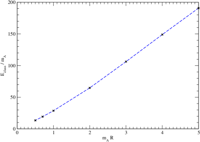
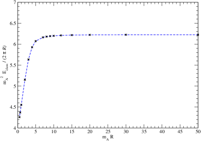
Figure 3: (Color online) Dependence of the total energy (left panel) and the energy per unit length (right panel) on the torus radius, at otherwise fixed parameters.

Next, we want to demonstrate that the torus configuration has a classical instability against shrinking into nothing ($R\to 0$). To see this, we leave the discretization parameters at their values in eq. (27) and fix $\beta=1$ (and $e^{2}=\frac{1}{2}$). In fig. 3, we see that the total energy is a linear function of the torus radius $R$ down to very small radii, of the order of a few Compton wave lengths. A better signal is obtained by studying the total energy per unit (core) length, $E/(2\pi R)$. As can be seen from the right panel in fig. 1, the energy per unit length saturates at a constant asymptotic value (which equals the energy per unit length of the NO string listed after eq. (11)), down to about $\hat{R}\lesssim 5$. For smaller radii, the interaction between opposite sides of the torus leads to a considerable drop in the energy per unit length (cf. density plots below). As a consequence, the total energy $E$ of the torus configuration decays more than linearly at small core radii $R\to 0$, which means that it is classically unstable.

We can also verify that the profiles are predominantly functions of $\tau$, with only a very small $\sigma$-modulation. This is shown in the left panel of figure 4 for the Higgs profile $f(\sigma,\tau)$ (the gauge boson behaves similarly). A notable variation with $\sigma$ is only visible at very small $\tau$ when $\sigma\approx 0$ (i.e. on the vertical axis near the origin). The right panel of fig. 4 demonstrates that the NO profiles obtained in the last section agree with the torus profiles in the limit $\hat{R}\gg 1$, provided that we identify the radius $r$ of the NO configuration, eq. (7), with the outer distance $2R/({\rm e}^{\tau}-1)$, cf. eq. (26).

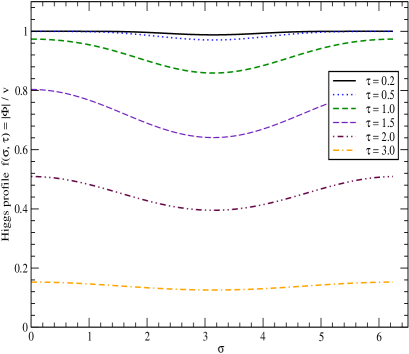
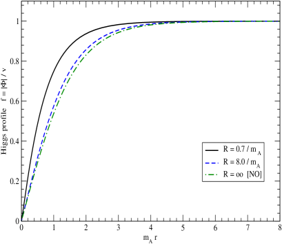
Figure 4: (Color online) Left panel: Higgs profile $f(\sigma,\tau)$ as a function of $\sigma$ for $\hat{R}=8.0$ and various values of $\tau$. Right panel: Comparison of the NO Higgs profile from section II with the profile from the torus configuration for two values of $\hat{R}$. Both charts refer to the model parameters $e^{2}=\frac{1}{2}$ and $\beta=1$. In the right panel the variable $r$ refers to $r$ as in eq. (7) for the NO string and to $2R/({\rm e}^{\tau}-1)$ for the closed string.

Finally, we visualize our configuration with density plots of the Higgs magnitude $|\Phi|/m_{A}\sim f(\sigma,\tau)$ in a plane perpendicular to the torus core. (The real configuration is found by rotating the 2D density plot around the vertical axis.) From the Higgs magnitude, we see the expected profiles for large radii, and the overlap in the inner region of the torus for very small radii. The other local quantities (magnetic field, energy density etc.) show a qualitatively similar behavior.

IV Quantum stabilization

We have seen above that the energy of the torus decreases linearly for a wide range of torus core radii $R$ (and even faster than linearly) at very small $R$), i.e. there is a classical instability of the torus configuration against shrinking into nothing. As argued from the uncertainty principle in the introduction, we expect that quantum effects will eventually stabilize the torus at a sufficiently small radius, so that a stable quantum torus configuration emerges.

IV.1 Quantum action for the instable mode

There are various ways to compute the relevant quantum corrections. In situations where the number of external degrees of freedom or quantum numbers is large, the leading corrections come from the small amplitude fluctuations, which can be efficiently computed using spectral methods Graham:2009zz , at least when there is sufficient symmetry to formulate a scattering problem. Formally, this correction is of order $\mathscr{O}(\hbar)$. In the present case, however, the instability occurs in a very specific channel, associated with the scale of the configuration. This strongly suggests that collective quantum fluctuations in this channel may be significant and eventually prevent the configuration from collapsing. To identify these quantum fluctuations, we promote the torus core radius $R$ to a dynamical variable by making it time-dependent, $R=R(t)$.

More precisely, we consider a time-independent field configuration $\Theta_{R}(\mathbf{x})$ (not necessarily the one that minimizes eq. (19)), where $\Theta$ stands for any of the fields in eq. (19). The subscript $R$ indicates that the configuration may depend implicitly (through its functional form) on the torus radius $R$. It is important to note that this dependence does not arise from the use of toroidal coordinates, which is merely a parameterization of the space point $\mathbf{x}$, but rather describes a parameter in the functional form of $\Theta_{R}$ which is independent of the coordinates used. If we now promote $R$ to a dynamical variable by scaling $R\to\lambda(t)R\equiv R(t)$, we obtain a time-dependent field configuration

$$\Theta(\mathbf{x},t)=\Theta_{R(t)}(\mathbf{x})\,,$$ (28)

where $\mathbf{x}$ is time-independent. The general form of the action associated with the collective coordinate $R(t)$ must be

$$S=\int d^{4}x\,\mathscr{L}[\Theta_{R(t)}]=\int dt\,\left[\frac{1}{2}\,u(R)\,\dot{R}^{2}-E(R)\right]\,.$$ (29)

Here, the dot indicates a time derivative and we have explicitly indicated that the functions $u$ and $E$ depend on the collective coordinate $R(t)$. In addition they also depend on the model parameters and the choice of profile functions. For a time-independent radius, the action reproduces the energy functional in eq. (19). Moreover, the time derivative $\dot{R}$ appears quadratically because of time-reversal invariance and because the Lagrangian has at most two field derivatives.

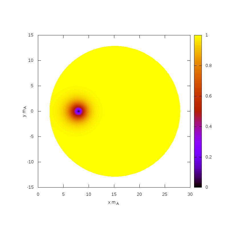
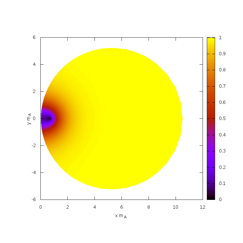
Figure 5: (Color online) Density plots of the Higgs magnitude in a plane perpendicular to the torus. All positions are in units of the gauge boson Compton wavelength $m_{A}^{-1}$. In the left panel, the torus has a radius $\hat{R}=m_{A}R=8$, while in the right panel shows results for $\hat{R}=0.7$. Notice the different scales on the axes in both cases.

The profile functions depend on the spatial coordinates only via the ratio $\mathbf{x}/R$ that defines the toroidal coordinates, cf. eq. (12). We elevate this radius to a time dependent variable. This time dependence produces non-zero time derivatives in the action, eq. (29), from which we read off the mass function $u(R)$. In addition to the scale dependence of the profile functions the fields may be subject to explicit scaling as well.

The vacuum expectation value of the Higgs fields is fixed at spatial infinity. Thus there is no explicit scaling in this case and the parameterization of the time dependent Higgs field becomes,

$$\phi(\mathbf{x},t)=\phi_{0}(\mathbf{x}/R(t))=\widetilde{\phi}_{0}(\sigma_{t},\tau_{t})\,.$$ (30)

While $\widetilde{\phi}_{0}(\sigma,\tau)$ is a prescribed profile function of toroidal coordinates, $\sigma_{t}$ and $\tau_{t}$ denote the particular toroidal coordinates for the scaled point $\mathbf{x}/R(t)$. Since we consider the field $\phi(\mathbf{x},t)$ at a given space point $\mathbf{x}$, we must treat the arguments of the profile function $\widetilde{\phi}_{0}$ as time-dependent variables. As we anticipated, this dependence induces a non-zero time derivative that is most conveniently computed from eq. (12) for $\varphi=0$, taking into account that $\partial\mathbf{x}/\partial t=0$:

$$\begin{pmatrix}\dot{\sigma}_{t}\cr\dot{\tau}_{t}\end{pmatrix}=-\frac{\dot{R}}{R}\left[\begin{pmatrix}\frac{\partial x}{\partial\sigma}&\frac{\partial x}{\partial\tau}\\[5.69054pt] \frac{\partial z}{\partial\sigma}&\frac{\partial z}{\partial\tau}\end{pmatrix}^{-1}\begin{pmatrix}x\cr z\end{pmatrix}\right]_{t}=\frac{\dot{R}}{R}\begin{pmatrix}\sin\sigma_{t}\,\cosh\tau_{t}\cr\cos\sigma_{t}\,\sinh\tau_{t}\end{pmatrix}\,.$$ (31)

The subscript on the square bracket indicates that the toroidal coordinates are to be taken at the time dependent values $\sigma=\sigma_{t}$ and $\tau=\tau_{t}$. Then the time derivative of the Higgs fields becomes

$$\dot{\phi}(\mathbf{x},t)=\frac{\dot{R}}{R}\left[\widetilde{\nabla}\widetilde{\phi}_{0}(\sigma,\tau)\right]_{t}$$ (32)

where we have defined the dimensionless radial derivative

$$\widetilde{\nabla}=\sin\sigma\,\cosh\tau\,\frac{\partial}{\partial\sigma}+\cos\sigma\,\sinh\tau\,\frac{\partial}{\partial\tau}\,,$$ (33)

which does not depend on the radius $R$. For the gauge field the situation is a bit more complicated because there is no boundary condition that disallows an overall scaling by an $R$ dependent function. In principle any parameterization would be allowed, because as a solution to the full field equations the correct $R$ dependence would be a result. However, we consider only a subset of these equations, specified by our ansatz. As for the NO string the field equations require that the covariant derivative vanishes as spatial infinity. On the other hand we do not want to abandon our choice $g(\sigma,\tau)\to 1$ for the boundary condition at $|\mathbf{x}|\to\infty$. Since the derivative induces a factor $1/R$ due to $\frac{\partial}{\partial\mathbf{x}}=\frac{1}{R}\frac{\partial}{\partial(\mathbf{x}/R)}$ we include exactly this factor in the parameterization of the gauge field

$$\mathbf{A}(\mathbf{x},t)=\frac{1}{R(t)}\,\widetilde{\mathbf{A}}_{0}(\sigma_{t},\tau_{t})$$ (34)

to ensure that the covariant derivative has a uniform scale dependence. This factor additionally contributes to the time derivative of the gauge field

$$\dot{\mathbf{A}}(\mathbf{x},t)=\frac{\dot{R}}{R^{2}}\left[(\widetilde{\nabla}-1)\,\widetilde{\mathbf{A}}_{0}(\sigma,\tau)\right]_{t}\,.$$ (35)

To obtain the Lagrange function, eq. (29), we need to integrate over coordinate space with the measure

$$d^{3}x=R^{3}d^{3}[x/R]=R^{3}\,d^{3}[\sigma_{t},\tau_{t},\varphi_{t}]$$ (36)

where the last expression refers to the integration measure of toroidal coordinates. After spatial integration the scale dependence factors as powers $R^{k}$ and the ratio $\dot{R}/R$. In summary, the ansätze for the field configuration together with their time derivatives are

$$\begin{array}[]{llll}\Phi(\mathbf{x},t)&=v\,{\rm e}^{in\sigma}f(\sigma,\tau)\,,&\dot{\Phi}(\mathbf{x},t)&=v\,{\rm e}^{in\sigma}\,\frac{\dot{R}}{R}\,\Big{[}inf(\sigma,\tau)\,\sin\sigma\,\cosh\tau+\widetilde{\nabla}f(\sigma,\tau)\Big{]}\,,\\[11.38109pt] \mathbf{A}(\mathbf{x},t)&=\frac{n}{e}\,\frac{{\scriptstyle g}(\sigma,\tau)}{R\,\eta(\sigma,\tau)}\,\mathbf{e}_{\sigma}\,,&\dot{\mathbf{A}}(\mathbf{x},t)&=\frac{n}{e}\,\frac{\dot{R}}{R}\,\Big{[}\widetilde{\nabla}-1\Big{]}\,\frac{{\scriptstyle g}(\sigma,\tau)}{R\,\eta(\sigma,\tau)}\,\mathbf{e}_{\sigma}\,.\end{array}$$ (37)

We have omitted the index on the toroidal coordinates because we have turned them into (dummy) integration variables, as in eq. (36). Also, we have not explicitly indicated the implicit dependence of the profiles on the radius induced by the stationary conditions. Note that to facilitate the numerical calculation, the scaling has been set up such that these profile functions obey exactly the boundary conditions discussed in section III.2.

The kinetic term $\dot{\mathbf{A}}^{2}$ for the gauge boson thus becomes

$$\dot{\mathbf{A}}^{2}=\left(\frac{n}{e}\right)^{2}\,\frac{\dot{R}^{2}}{2R^{4}\,\eta^{2}}\,\Big{[}\big{(}\cos(2\sigma)+\cosh(2\tau)\big{)}\,g^{2}+4\,\cos\sigma\,\cosh\tau g\widetilde{\nabla}g+2\,\big{(}\widetilde{\nabla}g\big{)}^{2}\Big{]}$$ (38)

IV.2 Gauß’ law

For time-dependent fields, the initial Lagrangian eq. (2) can be split into three pieces:

$$\mathscr{L} =\Big{\{}\frac{1}{2}\,\dot{\mathbf{A}}^{2}+|\dot{\Phi}|^{2}\Big{\}}+\Big{\{}\frac{1}{2}\,(\nabla A_{0})^{2}+e^{2}\,|\Phi|^{2}\,A_{0}^{2}-A_{0}\,\mathcal{J}_{0}\Big{\}}-\Big{\{}|\mbox{\boldmath$D$\unboldmath}\Phi|^{2}+V(\Phi)\Big{\}}$$

$$=\mathscr{L}_{\rm kin}+\mathscr{L}_{\rm gauss}+\mathscr{L}_{\rm stat}\,.$$ (39)

The $A_{0}$ field only appears in $\mathscr{L}_{\rm gauss}$, and this contribution gives rise to Gauß’ law, eq. (6), with the source

$$\mathcal{J}_{0}\equiv ie\,\Big{(}\dot{\Phi}\,\Phi^{\ast}-\dot{\Phi}^{\ast}\,\Phi\Big{)}+\nabla\dot{\mathbf{A}}\,.$$ (40)

In the static case, we had $\mathcal{J}_{0}=0$ and hence $A_{0}=0$ and $\mathscr{L}_{\rm gauss}=0$. This is no longer the case when the fields are time-dependent because of the dynamic scaling of the closed string. From $\dot{\Phi}$ in eq. (37), the Higgs contribution to the source $\mathcal{J}_{0}$ reads (recall $m_{A}=\sqrt{2}ev$)

$$ie\,\Big{(}\dot{\Phi}\,\Phi^{\ast}-\dot{\Phi}^{\ast}\,\Phi\Big{)}=-\frac{n}{e}\,m_{A}^{2}\,\frac{\dot{R}}{R}\,f^{2}\,\sin\sigma\,\cosh\tau\,.$$ (41)

The gauge field contribution to $\mathcal{J}_{0}$ is a bit more involved. Since our torus ansatz in eq. (16) is not transverse, we can either take the time derivative of eq. (17) following the rule (37), or take the divergence of $\dot{\mathbf{A}}$ in eq. (37). Using the identity $[\nabla,\widetilde{\nabla}]=-\nabla$, the result from both calculations is

$$\nabla\cdot\dot{\mathbf{A}}=\frac{n}{e}\,\frac{\dot{R}}{R^{3}}\,\big{(}\widetilde{\nabla}-2\big{)}\,\Big{[}\eta^{-3}\,\partial_{\sigma}(g\,\eta)\Big{]}\,.$$ (42)

From eqs. (41) and (42), we observe $\mathcal{J}_{0}\sim\dot{R}/e$ and hence $e\,A_{0}\sim\dot{R}$ due to the field equation (44). The time dependent scaling thus induces a temporal component of the gauge field that is proportional to the time derivative of the radius. It is thus suggestive to set

$$e\,A_{0}(\mathbf{x},t)=\frac{\dot{R}}{R}\,q(\sigma,\tau)\,,$$ (43)

with a dimensionless profile function $q$ that solves, in principle,

$$\Big{[}(-\Delta)+m_{A}^{2}f^{2}\Big{]}\,q=\mathcal{J}_{0}e\,\frac{R}{\dot{R}}\equiv\mathcal{Q}[f,g]\,.$$ (44)

Instead of solving eq. (44) directly, it is much more efficient to treat Gauß’ law on equal footing with the remaining field equations. That is, we keep $q$ as an independent field that appears in the contribution

$$\int d^{4}x\,\mathscr{L}_{q}=\int d^{4}x\,\frac{\dot{R}^{2}}{e^{2}\,R^{2}}\,\left[\frac{1}{2}\left((\nabla q)^{2}+m_{A}^{2}\,f^{2}\,q^{2}\right)-q\mathcal{Q}\right]\equiv\int dt\,\frac{1}{2}\,u_{q}(R)\,\dot{R}^{2}$$ (45)

to the kinetic energy in eq. (29). Since the remaining parts of the action are independent of $q$, the minimization of the action with respect to $q$ will minimize the kinetic term and thus $u_{q}$, which is equivalent to Gauß’ law eq. (44). The conclusion is that treating $f$, $g$, and $q$ as independent fields will automatically give the correct contribution to the (quantum) energy from Gauß’ law, provided that $q$ is determined from the minimization of $u_{q}(R)$.

If we now collect all the pieces from eqs. (37), (38) and (45), with $\mathcal{Q}$ determined from eqs. (41) and (42), the action for the collective coordinate $R$ will indeed be of the form (29). The static energy is then given by eq. (19) and the explicit form of the mass term reads

$$\hat{u}(\hat{R})\equiv\frac{u(R)}{m_{A}}=\frac{2\pi}{e^{2}}\, \int\limits_{0}^{\infty}d\tau\int\limits_{-\pi}^{\pi}d\sigma\,\sinh\tau\Bigg{\{}\frac{n^{2}}{2\hat{R}}\,\eta\,\mathcal{M}[g]+\hat{R}\,\eta^{3}\,\mathcal{T}[f]+$$

$$+\hat{R}\,f^{2}\,\eta^{3}\,q^{2}+\frac{\eta}{\hat{R}}\,\left[(\partial_{\sigma}q)^{2}+(\partial_{\tau}q)^{2}\right]-2\hat{R}\,\eta^{3}\,\mathcal{K}[f,g]q\Bigg{\}}\,.$$ (46)

The explicit form of the local expressions $\mathcal{M}$, $\mathcal{T}$ and $\mathcal{K}\equiv\mathcal{Q}/m_{A}^{2}$ can be found in appendix .3. To discuss the boundary conditions for $q(s,t)$, it is convenient to rewrite eq. (46) in the form

$$\hat{u}(\hat{R})=\frac{2\pi}{e^{2}}\,\int\limits_{0}^{\infty}dt\int\limits_{-\pi}^{\pi}d\sigma\,\sinh\tau\Bigg{\{} \frac{n^{2}}{2\hat{R}}\,\eta\,\mathcal{M}[g]+\hat{R}\,\eta^{3}\,\Big{[}(\widetilde{\nabla}f)^{2}-2q\,\frac{n}{\hat{R}^{2}}\,\big{(}\widetilde{\nabla}-2\big{)}\,\big{[}\eta^{-3}\,\partial_{\sigma}(g\,\eta)\big{]}\Big{]}+$$

$$+\frac{n}{\hat{R}}\,\left[(\partial_{\sigma}q)^{2}+(\partial_{\tau}q)^{2}\right]+\hat{R}\,\eta^{3}\,\Big{[}n\,\sin\sigma\,\cosh\tau+q\Big{]}^{2}\,f^{2}\Bigg{\}}\,.$$ (47)

At very small and very large $\tau$, the first line in this equation is suppressed because either the derivative of the profiles $f$ and $g$, or the profiles themselves vanish. The boundary conditions for $q$ are thus determined from the balancing of the two terms in the second line of eq. (47). At $\tau\to 0$, we have $f\to 1$ by the classical equation of motion, and the last term in eq. (47) dominates. This limit thus yields the estimate $q\approx-n\sin\sigma\,\cosh\tau$, which is compatible with the Neuman boundary condition

$$\frac{\partial q(s,t)}{\partial\tau}\Big{|}_{\tau\to 0}=0$$ (48)

also obeyed by the other profiles $f$ and $g$. At $\tau\to\infty$, we have $f\to 0$ by the boundary conditions and thus the first term in the second line of eq. (47) dominates, which also yields a Neumann boundary condition

$$\frac{\partial q(s,t)}{\partial\tau}\Big{|}_{\tau\to\infty}=0\,.$$ (49)

While this result differs from the Dirichlet condition eq. (22) obeyed be the other profiles, the numerical studies below indicate that $q(s,\infty)\approx 0$ when the field equations are obeyed (at the end of the $q$-relaxation).

IV.3 Quantization of the collective coordinate

Up to now, we have only determined the action (29) due to the unstable mode $R(t)$. To compute the quantum correction to the energy due to this mode, we next have to quantize this model. First, we note that the mass term $\hat{u}(\hat{R})$ is coordinate-dependent, so we have to introduce a metric factor $g_{11}=\hat{u}(\hat{R})$ with $g={\rm det}(g)=|\hat{u}(\hat{R})|$. The generalized canonical momentum from the classical action eq. (29) is

$$p\equiv\hat{u}(\hat{R})\,\frac{d\hat{R}}{d\hat{t}}\,.$$

The coordinate $\hat{R}$ requires an extra connection (Christoffel symbol, $\Gamma=\frac{1}{2g}\frac{\partial g_{11}}{\partial\hat{R}}$) upon quantization

$$p=-i\hbar\,\left(\frac{\partial}{\partial\hat{R}}+\frac{1}{2}\,\Gamma\right)=-i\hbar\,\left(\frac{\partial}{\partial\hat{R}}+\frac{1}{4}\,\frac{\hat{u}^{\prime}(\hat{R})}{\hat{u}(\hat{R})}\right)\,.$$

This quantized momentum obeys the canonical commutation relations $[\hat{R},p]=i\hbar$ and the Hamilton operator of the model (29) becomes

$$H=\frac{1}{2}\,g^{-\nicefrac{{1}}{{4}}}\,p\,g^{\nicefrac{{1}}{{2}}}\,g^{11}\,p\,g^{-\nicefrac{{1}}{{4}}}+\hat{E}(\hat{R})=\frac{\widetilde{p}^{2}}{2}+\hat{E}(\hat{R})\,,$$ (50)

where the transformed momentum is $\widetilde{p}\equiv\hat{u}^{-\nicefrac{{1}}{{4}}}\,p\,\hat{u}^{-\nicefrac{{1}}{{4}}}\,.$

In principle, we would have to find the ground state energy $E_{0}$ of the Hamiltonian in eq. (50), for given background profiles $f(\sigma,\tau)$ and $g(\sigma,\tau)$ (with $q(\sigma,\tau)$ constructed from eq. (44)), and then minimize $E_{0}$ rather than eq. (19). This is very expensive computationally, because we need to solve for $E_{0}$ at every step of the relaxation, which means solving a variational problem for a highly non-local functional. As motivated earlier we will follow a simpler approach: From the definition of $\widetilde{p}$ and $p$, we find the commutator

$$\big{[}\,\widetilde{p}\,,\,\hat{R}\,\big{]}=-i\hbar\,\hat{u}^{-\nicefrac{{1}}{{2}}}\,,$$

and therefore the general uncertainty relation in an arbitrary state $\psi$,

$$\sigma_{\psi}(\widetilde{p})^{2}\,\sigma_{\psi}(\hat{R})^{2}\geq\frac{\hbar^{2}}{4}\,\left|\big{\langle}\psi\,|\,\hat{u}^{-\nicefrac{{1}}{{2}}}\,|\,\psi\big{\rangle}\right|^{2}\,.$$ (51)

Initially, the Hamiltonian and the wave functions are only defined for $\hat{R}>0$, with a potential singularity at $\hat{R}=0$ that is avoided self-consistently. Formally, we can then extend $H$ and $\psi$ to negative $\hat{R}$ in such a way that parity is conserved and the ground state $\psi_{0}$ is symmetric. As a consequence $\big{\langle}\,\psi_{0}\,\big{|}\,\widetilde{p}\,\big{|}\,\psi_{0}\,\big{\rangle}=\big{\langle}\,\psi_{0}\,\big{|}\,\hat{R}\,\big{|}\,\psi_{0}\,\big{\rangle}=0$ and eq. (51) becomes

$$\big{\langle}\,\psi_{0}\,\big{|}\,\widetilde{p}^{2}\,\big{|}\,\psi_{0}\,\big{\rangle}\geq\frac{\hbar^{2}}{4\,\big{\langle}\,\psi_{0}\,\big{|}\,\hat{R}^{2}\,\big{|}\,\psi_{0}\,\big{\rangle}}\,\left|\big{\langle}\psi_{0}\,|\,\hat{u}^{-\nicefrac{{1}}{{2}}}\,|\,\psi_{0}\big{\rangle}\right|^{2}\,.$$

Next we assume that the ground state $\psi_{0}$ is localized such that $\hat{R}$ is restricted to an effective range $-\hat{R}_{0}\lesssim\hat{R}\lesssim\hat{R}_{0}$, so that

$$\big{\langle}\,\psi_{0}\,\big{|}\,\hat{R}^{2}\,\big{|}\,\psi_{0}\,\big{\rangle}\approx\frac{\hat{R}_{0}^{2}}{4}\quad{\rm and}\quad\left|\big{\langle}\psi_{0}\,|\,\hat{u}^{-\nicefrac{{1}}{{2}}}\,|\,\psi_{0}\big{\rangle}\right|^{2}\approx u(\hat{R}_{0})^{-1}\,.$$

Using this in the previous equation gives

$$\big{\langle}\,\psi_{0}\,\big{|}\,\widetilde{p}^{2}\,\big{|}\,\psi_{0}\,\rangle\approx\frac{\hbar^{2}}{\hat{u}(\hat{R}_{0})\,\hat{R}_{0}^{2}}\,.$$

Then the ground state energy is well approximated by

$$\hat{E}_{0}=\big{\langle}\,\psi_{0}\,\big{|}\,H\,\big{|}\,\psi_{0}\,\big{\rangle}\approx\frac{\hbar^{2}}{2\,\hat{u}(\hat{R}_{0})\,\hat{R}_{0}^{2}}+\big{\langle}\,\psi_{0}\,\big{|}\,\hat{E}(\hat{R})\,\big{|}\,\psi_{0}\,\big{\rangle}\approx\frac{\hbar^{2}}{2\,\hat{u}(\hat{R}_{0})\,\hat{R}_{0}^{2}}+\hat{E}(\hat{R}_{0})\,.$$ (52)

In principle, $\hat{R}_{0}$ is the radius of the region where the ground state is localized. For a fixed externally prescribed radius $\hat{R}$, the ground state will adapt and localize around $\hat{R}_{0}\approx\hat{R}$. This allows to re-interpret eq. (52): For an externally prescribed core radius $\hat{R}$, the quantum system is localized near $\hat{R}$. As with any quantum system, it reacts to the localization with quantum fluctuations that are repulsive at very small distances. These fluctuations compete with the classical energy $\hat{E}(\hat{R})$, which favors $\hat{R}\to 0$ according to the instability observed in section IV. These two effects balance and the system stabilizes at the minimum of the quantum energy

$$\hat{E}_{q}\approx\frac{1}{2}\,\frac{\hbar^{2}}{\hat{u}(\hat{R})\,\hat{R}^{2}}+\hat{E}(\hat{R})\,.$$ (53)

This quantum energy differs from the classical energy by the contribution from the quantization of the unstable mode. We assume that this contribution is the dominant quantum effect in stabilizing the closed string configuration against shrinking to zero.

The derivation of equation (53) involved various approximations, but a full quantum mechanical treatment is likely to produce something similar — maybe with a numerical factor of order one in the quantum correction — because the derived form of the quantum corrected energy is essentially dictated by fundamental principles of quantum mechanics. For a first estimate and a proof of principle of quantum stabilization, eq. (53) therefore represents a completely adequate starting point.

IV.4 Numerics

For the numerical minimization of the quantum energy in eq. (53), we employ the relaxation technique presented in the last section as follows: We

1. determine the profiles $f$ and $g$ by minimizing the classical energy $\hat{E}(\hat{R})$ from eq. (19);

2. compute the auxiliary field $q$ by minimizing the ($q$-dependent part of the) collective mass function $u_{q}$ in eq. (46) (see appendix .4 for explicit expressions, in analogy to eq. (25) $q_{st}$ is the discretized version form of $q(\sigma,\tau)$),

   $$\frac{\delta\hat{u}}{\delta q_{st}} =\frac{4\pi}{e^{2}}\,\sinh(\tau_{0}+t\Delta_{t})\,\Big{[}X_{st}\,q_{st}-Y_{st}\Big{]}\stackrel{{\scriptstyle!}}{{=}}0\,;$$ (54)

3. compute the quantum energy $\hat{E}_{q}(\hat{R})$ from eq. (53) by substituting the profiles from 1) and 2).

These operations are performed for each fixed radius $\hat{R}$ separately. Minimization of the total quantum energy, $\hat{E}_{q}$ from eq. (53), would require us to re-adjust the profiles $f$ and $g$ after running through steps 1)-3). This procedure would then have to be iterated to convergence since modifying the profiles $f$ and $g$ causes $q$ to change as well. Alternatively, we could relax all fields $f$, $g$ and $q$ simultaneously using $\hat{u}_{q}$ as target functional for the minimization of $q$ and $\hat{E}_{q}$ as target functional for $f$ and $g$. In both cases, the minimization of $\hat{E}_{q}$ would be performed with the relaxation condition

$$\delta\hat{E}_{q}=-\frac{\hbar^{2}}{2\hat{u}^{2}\,\hat{R}^{2}}\,\delta\hat{u}+\delta\hat{E}=0\,.$$ (55)

Since $\hat{u}$ is at most quadratic in the profiles $f$ and $g$, the variation $\delta\hat{u}$ is at most linear. Hence the quantum correction in the relaxation condition (55) affects the coefficients $H_{st}$, $L_{st}$ (for $f$), and $A_{st}$, $B_{st}$ (for $g$), cf. appendix .2. Obviously these corrections are proportional to $1/\hat{u}^{2}$ and thus heavily suppressed since our numerical studies below yield $\hat{u}>100$ for all radii at the minimum, and even much larger during relaxation. Therefore the impact of the quantum correction on the profiles $f$ and $g$ is a negligible higher order effect and the simple procedure 1)-3) listed above is essentially equivalent to the complete minimization of $E_{q}$ within our numerical accuracy.

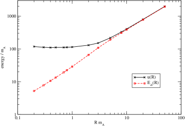
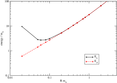
Figure 6: (Color online) Left panel: Mass factor of the collective coordinate and classical energy, as a function of the torus radius. Right panel: Quantum energy vs. classical energy as a function of the torus radius. All simulations were performed with the standard parameters $e^{2}=1/2$ and $\beta=1$.

Figure 6 shows the numerical results for the mass function eq. (46) for the collective mode using the profiles obtained according to steps 1) and 2). For large and moderate radii $R$, the mass is fairly close to the classical energy, and decreases accordingly when $R$ decreases. If this trend continued down to very small radii, we would observe quantum stabilization at the expected torus size of a few Compton wave lengths, $\hat{R}\approx 1$. However, figure 1 shows that the mass function starts to saturate at around $\hat{R}\approx 5$ at a large value of $\hat{u}\approx 110$. As a consequence, the stabilizing radius $\hat{R}\approx 0.1$ in the right panel of figure 6 is about one order of magnitude smaller than naïvely expected. Although the stabilizing mechanism works in principle, the geometry of the stable configuration is characterized by such a small radius that it no longer resembles a torus. It is suggestive that other quantum effects may have already become relevant for such configurations.

A more thorough understanding of the numerical results for $\hat{u}$ is gained by separating three contributions in eq. (46): The first two terms are the gauge and Higgs kinetic energies, respectively. The third contribution implements Gauß’ law. Table 2 shows some typical results: The gauge kinetic energy accounts for about one third of the total mass, while the Higgs kinetic energy and Gauß’ law give very large contributions that almost cancel each other. In total these two pieces constitute approximately two thirds of the mass. On the other hand, if we separate contributions according to eq. (47) no cancellation of large terms emerges. The reason is that those terms are organized as the square of the covariant derivative, $|D_{0}\Phi|^{2}$. In that combination Gauß’ law guarantees that there are no large canceling contributions to the integral from spatial infinity. If we had not solved Gauß’ law, a non-zero Higgs field contribution to the mass function at spatial infinity would not be canceled and the mass function would be ill-defined. This is reflected by the (almost linear) increase of the Higgs field component displayed in table 2.

$\hat{R}=R/m_{A}$	gauge	Higgs	Gauß	total
$50.0$	415.0	227075.0	-225504.0	1985.8
$20.0$	167.3	90108.0	-89477.2	798.1
$10.0$	86.0	44783.1	-44463.3	388.7
$8.0$	70.2	35757.6	-35499.2	310.0
$5.0$	47.8	22260.0	-22091.4	216.5
$3.0$	36.2	13304.9	-13189.9	151.2
$2.0$	33.5	8856.5	-8759.6	130.4
$1.0$	32.3	4435.2	-4353.3	114.2
$0.8$	32.3	3555.9	-3476.3	111.9
$0.5$	32.8	2243.4	-2164.9	111.2
$0.3$	31.7	1323.4	-1242.5	112.5

Table 2: Contributions to the mass function eq. (46) for the collective coordinate, as a function of the torus radius. Data was taken on $350\times 350$ lattices at the standard parameters $e^{2}=1/2$ and $\beta=1$.

The accurate determination of the mass factor eq. (46) requires a high resolution in the (tiny) region between the torus core at $R$ and the origin. In addition, the overall grid extension must be large enough to reach asymptotic distances. The numerical parameter $d_{\rm max}$, which controls both the extension towards spatial infinity and the distance from the symmetry axis, is measured in units of $R$. On the other hand, the physical length scale is the Compton wave length, $1/m_{A}$. Hence $d_{\rm max}$ has to be very large, especially when $\hat{R}<1$. In practice, values of $d_{\rm max}\simeq 200$ and grid sizes up to $500\times 500$ were necessary to obtain stable results.

For completeness, we have plotted the induced profile function $q$, that emerges from Gauß’ law for two different radii in figure 7. Deviations from the vacuum value $q=0$ extend much further out from the core region than the profiles $f$ and $g$, cf. figure 5. Also, the main structure is located above and below the plane of the torus (core line) and $q$ changes sign across this plane. The $q$-field vanishes in the core plane, which is not implemented as a boundary condition, cf. eq. (49), but rather a result obtained when the relaxation has converged and thus it is a consequence of Gauß’ law.

For very small radii, rather large values of $d_{\rm max}$ are required in order to cover the region near the vertical axis in figure 7, in which the deviation from the vacuum is sizeable. For illustration purposes $d_{\rm max}$ has been chosen fairly small ($d_{\rm max}\approx 10$) in figure 7 while in the actual numerical calculations it was taken at least an order of magnitude larger.

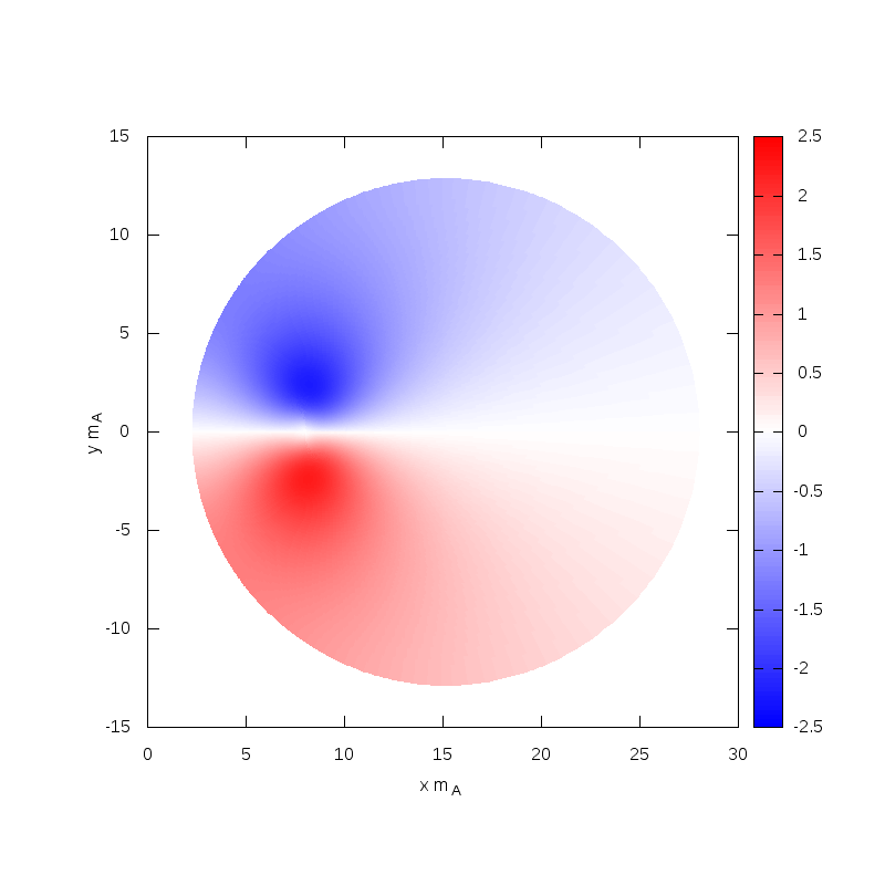
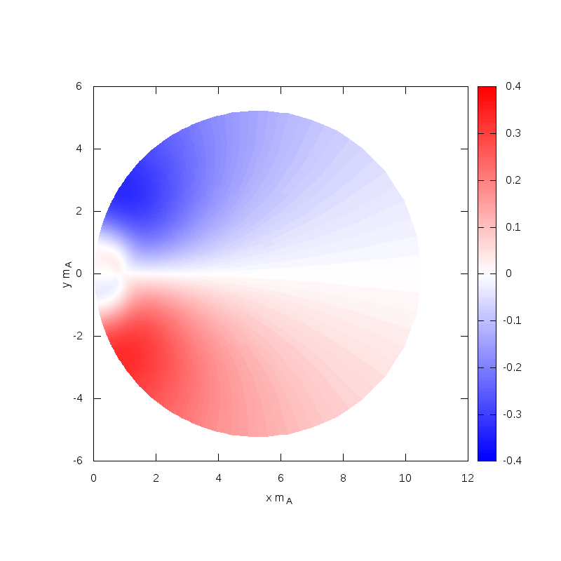
Figure 7: (Color online) Density plots of the profile function $q$ in a plane perpendicular to the torus. In the left panel, the torus has a radius $\hat{R}=8$, while in the right panel shows results for $\hat{R}=0.7$. Notice the different scales on the axes in both cases. The profile is positive (negative) in the lower (upper) half-plane.

V Conclusion

The Nielsen-Olesen string in scalar electrodynamics is a suitable toy model for cosmic strings in non–Abelian gauge theories such as the Standard Model. For this reason we have investigated the stability issue of the closed Nielsen-Olesen string. The closed string has been constructed by introducing toroidal coordinates. This complicated matters significantly because the profiles become functions of two independent variables, and quantitative analyses cannot be pursued in from of ordinary differential equations. Therefore we adopted a lattice approach and performed variational calculations by relaxation methods. This verified the classical instability of a toroidal string as the closed string shrinks to size zero. As in the case of the classical hydrogen atom, by radiating energy as fluctuations and simultaneously shrinking, the closed string will eventually decay.

In the context of the cosmological assumption that large scale closed cosmic strings could have existed at early times, this analysis suggests that (non-interacting) closed strings would not have survived. We have then argued that quantum mechanics in form of the uncertainty principle disallows objects that at some stage possessed a finite size squeeze to arbitrarily small extensions. Motivated by this observation we have developed a formalism for the quantum stabilization. It is based on the uncertainty principle and inspired by its success in reproducing the fundamental quantum mechanical properties of the hydrogen atom.

Technically this approach requires the computation of an inertia function for a time dependent radius of the string. This inertia function can be interpreted as a mass for the radius of the torus and we have estimated its kinetic energy term in the quantum energy functional. We have then applied a variational principle to this functional (appropriately extending the configuration manifold properly to implement Gauß’ law) and determined the field configuration from the minimal quantum energy at a prescribed radius. As expected from the uncertainty principle, the kinetic energy part is negligible for large radii. More surprisingly, it is also quite small for radii that are of the scale of the Compton wave-length of the fundamental fields. Nevertheless we have observed that the proposed mechanism of quantum stabilization is indeed operative in the case of the closed Nielsen-Olesen string as the quantum energy exhibits a global minimum for a non-zero radius. The proper incorporation of Gauss’ law proved essential for this mechanism to work. However, the numerical results for the radius at at which the torus becomes stable suggest that other mechanisms should be relevant as well, since this radius is about an order of magnitude smaller than the length-scale inherent in the model. (We do not expect the corrections to the approximations in section IV.3 to compensate for this.) At such small radii the toroidal character of the shrinking configuration has disappeared and presumably additional quantum modes (besides the length scale) must be included when computing the quantum energy. This conclusion is further supported by the fact that the mass associated with the radial mode is quite large. Hence the spectrum of radial excitations will be very dense. Presumably these additional quantum fluctuations will be enhanced in the interior region of the string. Rather than decaying to infinity, these fluctuations would increase the energy of the string thereby stabilizing it at radii larger than those computed here. This suggests that the stabilization radius obtained from the application of the uncertainty principle to the radius of the closed string is merely a lower limit. Of course, due to the complicated structure of the background configuration any quantitative analysis of this scenario will be a formidable task.

Appendices

In these appendices we present details of the numerical approach used in sections III and IV.

.1 Lattice discretization

We start with the discretized description eq. (24), where the profiles turn into real functions

$$f_{st}\equiv f(s\,\Delta_{s},\tau_{0}+t\,\Delta_{t})\,,\qquad\qquad g_{st}\equiv g(s\,\Delta_{s},\tau_{0}+t\,\Delta_{t})$$ (56)

defined on the lattice sites. The boundaries of the parameter regions are at $t=0$ and $t=N_{t}$, and at $s=0$ and $s=N_{s}$, respectively, where we impose the following conditions, cf. eqs. (22)–(21):

• periodic boundary conditions on $s$:

  $$f_{0t}=f_{N_{s}t}\,,\qquad\qquad g_{0t}=g_{N_{s}t}\,,\qquad\quad t\in\{0,\ldots,N_{t}\}$$ (57)

• Dirichlet conditions at $t=N_{t}$:

  $$f_{sN_{t}}=0\,\qquad\qquad g_{sN_{t}}=0\,,\qquad\qquad\quad s\in\{0,\ldots\,N_{s}\}$$ (58)

• Neumann conditions at $t=0$:

  $$f_{s0}=f_{s1}\,,\qquad\qquad g_{s0}=g_{s1}\,,\qquad\qquad s\in\{0,\ldots,N_{s}\}\,.$$ (59)

Notice that the derivatives in the Neumann conditions are forward derivatives at $t=0$ so that no extra grid points are required. For integrals over $s$ and $t$, we use the same prescription combined with a left Riemann sum definition,

$$\int\limits_{\tau_{0}}^{\tau_{\infty}}d\tau\,u(\tau)\to\sum_{t=0}^{N_{t}-1}\Delta_{t}\,u(\tau_{0}+t\,\Delta_{\tau})\,.$$

This ensures that we will never encounter grid points outside the range defined in eq. (24). Next, we choose the discretized profiles $f_{st}$ and $g_{st}$ such as to minimize the (discretized) target functional eq. (19),

$$\hat{E} = \frac{\pi}{e^{2}}\sum_{t=0}^{N_{t}-1}\sum_{s=0}^{N_{s}-1}\Delta_{t}\Delta_{s}\,\sinh(\tau_{0}+t\Delta_{t})\,\Bigg{\{}\frac{n^{2}}{\hat{R}}\,\frac{1}{\eta_{st}}\,\left[\frac{g_{s,t+1}-g_{st}}{\Delta_{t}}\right]^{2}+$$

$${}+\hat{R}\,\eta_{st}\,\left[\left(\frac{f_{s,t+1}-f_{st}}{\Delta_{t}}\right)^{2}+n^{2}f_{st}^{2}(1-g_{st})^{2}+\left(\frac{f_{s+1,t}-f_{st}}{\Delta_{s}}\right)^{2}\right]+\frac{\beta}{4}\,\hat{R}^{3}\,\eta_{st}^{3}\,(1-f_{st}^{2})^{2}\Bigg{\}}\,,$$

where the dimensionless metric factor is given in eq. (20). Once the solutions $f_{st}$ and $g_{st}$ are found, the original profiles $f(\mathbf{x})$ and $g(\mathbf{x})$ can be restored from eq. (56) and the definition of toroidal coordinates, eq. (12).

.2 Relaxation

For the relaxation condition, we consider an interior point $(s,t)$ at which the profiles are not fixed by boundary conditions. At these points we can independently vary the profile functions and compute the associated gradients. We start by listing the result for the gauge field:

$$\frac{\delta\hat{E}}{\delta g_{st}}=\frac{2\pi}{e^{2}}n^{2}\,\sinh(\tau_{0}+t\Delta_{t})\,\Big{[}A_{st}\,g_{st}-\,B_{st}\Big{]}$$ (61)

with

$$A_{st} = \frac{\varepsilon}{\hat{R}}\,\left(\frac{1}{\eta_{st}}+\frac{\xi_{t}}{\eta_{s,t-1}}\right)+\hat{R}\,f_{st}^{2}\,\eta_{st}\,\Delta^{2}\,,$$

$$B_{st} = \frac{\varepsilon}{\hat{R}}\,\left(\frac{g_{s,t+1}}{\eta_{st}}+\xi_{t}\,\frac{g_{s,t-1}}{\eta_{s,t-1}}\right)+\hat{R}\,f_{st}^{2}\,\eta_{st}\,\Delta^{2}\,.$$

For later convenience, we have introduced the abbreviations

$$\xi_{t} \equiv \frac{\sinh(\tau_{0}+(t-1)\,\Delta_{t})}{\sinh(\tau_{0}+t\Delta_{t})}=\cosh(\Delta_{t})-\coth(\tau_{0}+t\Delta_{t})\,\sinh(\Delta_{t})\,,$$

$$\varepsilon \equiv \frac{\Delta_{s}}{\Delta_{t}}\qquad{\rm and}\qquad\Delta^{2}\equiv\Delta_{s}\,\Delta_{t}\,.$$

The local minimization of $\hat{E}$ with respect to $g_{st}$ yields the updating rule (relaxation condition)

$$g_{st}\longrightarrow\frac{B_{st}}{A_{st}}\,,$$ (62)

which in view of $A_{st}>0$ is a minimum. For the Higgs profile, $f_{st}$, a similar calculation gives

$$\frac{\delta\hat{E}}{\delta f_{st}}=\frac{2\pi}{e^{2}}\,\sinh(\tau_{0}+t\Delta_{t})\,\hat{R}\,\Big{[}2G_{st}\,f_{st}^{3}+H_{st}\,f_{st}-L_{st}\Big{]}\,,$$ (63)

with the coefficients

$$G_{st} = \frac{\beta}{4}\,\hat{R}^{2}\,\eta_{st}^{3}\,\Delta^{2}\,,$$

$$H_{st} = \varepsilon\,\left(\eta_{st}+\eta_{s,t-1}\,\xi_{t}\right)+\frac{1}{\varepsilon}\,\left(\eta_{st}+\eta_{s-1,t}\right)+n^{2}\,\eta_{st}\,(1-g_{st})^{2}\,\Delta^{2}-\frac{\beta}{2}\,\hat{R}^{2}\,\eta_{st}^{3}\,\Delta^{2}\,,$$

$$L_{st} = \varepsilon\left(f_{s,t+1}\,\eta_{st}+f_{s,t-1}\,\eta_{s,t-1}\,\xi_{t}\right)+\frac{1}{\varepsilon}\left(f_{s+1,t}\,\eta_{st}+f_{s-1,t}\,\eta_{s-1,t}\right)\,.$$

These values are such that the relaxation condition, $\frac{\delta\hat{E}}{\delta f_{st}}=0$, always has a real solution $f_{st}^{(0)}$ which can be computed by a closed formula into which we substitute the numerically obtained data for the coefficients $G_{st}$, $H_{st}$ and $L_{st}$. The updating rule for the Higgs field is then

$$f_{st}\longrightarrow f_{st}^{(0)}\,.$$ (64)

Since the relaxation conditions (62) and (64) only compute a local minimum with all other field variables held fixed, we must proceed iteratively and sweep through the entire lattice many times to relax to an overall stable minimum.

.3 Mass factor for the collective coordinate

The action for the collective coordinate $R$, eq. (29), contains a mass factor $u$ that is a local functional of the profiles. The three abbreviations in the explicit form eq. (46) read

$$\mathcal{M} =\big{(}\cos(2\sigma)+\cosh(2\tau)\big{)}\,g^{2}+4\,\cos\sigma\,\cosh\tau\,g\widetilde{\nabla}g+2\,\big{(}\widetilde{\nabla}g\big{)}^{2}$$

$$\mathcal{T} =(\widetilde{\nabla}f)^{2}+\left(n\,f\,\sin\sigma\,\cosh\tau\right)^{2}$$

$$\mathcal{K} =-n\,f^{2}\,\sin\sigma\,\cosh\tau+\frac{n}{\hat{R}^{2}}\,\big{(}\widetilde{\nabla}-2\big{)}\,\left[\eta^{-3}\,\partial_{\sigma}(g\,\eta)\right]\,.$$ (65)

Note that the profile functions $f$ and $g$ depend on the toroidal coordinates $\sigma$ and $\tau$. They also have an implicit dependence on the torus radius $R$.

.4 Quantum relaxation condition

The relaxation condition for the auxiliary field $q_{st}$ related to Gauß’ law was given in eq. (54) in the main text. The corresponding coefficients read explicitly

$$X_{st} =\hat{R}\,\eta_{st}^{3}\,f_{st}^{2}\,\Delta^{2}+\frac{1}{\hat{R}}\,\Big{[}\xi_{t}\,\epsilon\,\eta_{s,t-1}\,+\frac{1}{\epsilon}\,\eta_{s-1,t}+\left(\epsilon+\frac{1}{\epsilon}\right)\,\eta_{st}\Big{]}$$

$$Y_{st} =\hat{R}\,\eta_{st}^{3}\,\mathcal{K}_{st}\,\Delta^{2}+\frac{1}{\hat{R}}\,\Big{[}\epsilon\,\xi_{t}\,\eta_{s,t-1}\,q_{s,t-1}+\frac{1}{\epsilon}\,\eta_{s-1,t}\,q_{s-1,t}+\epsilon\,\eta_{st}\,q_{s,t+1}+\frac{1}{\epsilon}\,\eta_{st}\,q_{s+1,t}\Big{]}\,,$$ (66)

where $\mathcal{K}_{st}$ is the descretized (lattice) version of $\mathcal{K}$ in eq. (65).

References

- (1) M.B. Hindmarsh and T.W.B. Kibble, Rept. Prog. Phys. 58 (1994) 477.
- (2) T.W.B. Kibble, J. Phys. A 9 (1976) 1387.
- (3) A. Vilenkin and E.P.S. Shellard, Cosmic Strings and other Topological Defects, Cambridge University Press, Cambridge (UK), 1994.
- (4) A. Achucarro and C. J. A. Martins, arXiv:0811.1277 [astro-ph].
- (5) E. J. Copeland and T. W. B. Kibble, Proc. Roy. Soc. Lond. A 466 (2010) 623.
- (6) H. B. Nielsen and P. Olesen, Nucl. Phys. B 61 (1973) 45.
- (7) Y. Nambu, Nucl. Phys. B 130 (1977) 505.
- (8) T. Vachaspati, Phys. Rev. Lett. 68 (1992) 1977 [Erratum-ibid. 69 (1992) 216].
- (9) S. G. Naculich, Phys. Rev. Lett. 75 (1995) 998.
- (10) A. Achucarro and T. Vachaspati, Phys. Rept. 327 (2000) 347.
- (11) M. Groves and W. B. Perkins, Nucl. Phys. B 573 (2000) 449.
-
(12)
G. Starkman, D. Stojkovic, and T. Vachaspati,
Phys. Rev. D 65 (2002) 065003.
G. Starkman, D. Stojkovic, and T. Vachaspati, Phys. Rev. D 63 (2001) 085011.
D. Stojkovic, Int. J. Mod. Phys. A 16S1C (2001) 1034. - (13) M. Bordag and I. Drozdov, Phys. Rev. D 68 (2003) 065026.
- (14) N. Graham, V. Khemani, M. Quandt, O. Schröder, and H. Weigel, Nucl. Phys. B 707 (2005) 233.
- (15) N. Graham, M. Quandt, O. Schröder, and H. Weigel, Nucl. Phys. B 758 (2006) 112.
- (16) O. Schröder, N. Graham, M. Quandt, and H. Weigel, J. Phys. A 41 (2008) 164049.
- (17) J. Baacke and N. Kevlishvili, Phys. Rev. D 78 (2008) 085008.
- (18) M. Lilley, F. Di Marco, J. Martin, and P. Peter, Phys. Rev. D 82 (2010) 023510.
- (19) H. Weigel, M. Quandt, N. Graham, and O. Schröder, Nucl. Phys. B 831 (2010) 306.
- (20) H. Weigel and M. Quandt, Phys. Lett. B 690 (2010) 514.
- (21) H. Weigel, M. Quandt, and N. Graham, Phys. Rev. Lett. 106 (2011) 101601.
- (22) N. Graham, M. Quandt, and H. Weigel, Phys. Rev. D 84 (2011) 025017 [arXiv:1105.1112 [hep-th]].
- (23) E. Witten, Nucl. Phys. B 249 (1985) 557.
- (24) R. L. Davis and E. P. S. Shellard, Nucl. Phys. B 323 (1989) 209.
-
(25)
A. Vilenkin,
Phys. Rev. Lett. 46 (1981) 1169
[Erratum-ibid. 46 (1981) 1496].
A. Vilenkin, Phys. Rev. D 24 (1981) 2082. -
(26)
T. W. B. Kibble and N. Turok,
Phys. Lett. B 116 (1982) 141.
T. W. B. Kibble, Nucl. Phys. B 252 (1985) 227 [Erratum-ibid. B 261 (1985) 750]. - (27) C. J. Burden, Phys. Lett. B 164 (1985) 277.
- (28) J. J. Blanco-Pillado, K. D. Olum, and B. Shlaer, Phys. Rev. D 83 (2011) 083514 [arXiv:1101.5173 [astro-ph.CO]].
- (29) R. L. Davis, Phys. Rev. D 38 (1988) 3722.
- (30) R. L. Davis and E. P. S. Shellard, Phys. Lett. B 209 (1988) 485.
- (31) A. C. Davis and P. Peter, Phys. Lett. B 358 (1995) 197.
- (32) A. C. Davis and W. B. Perkins, Phys. Lett. B 390 (1997) 107.
- (33) S. C. Davis, W. B. Perkins, and A. C. Davis, Phys. Rev. D 62 (2000) 043503.
-
(34)
Y. Lemperiere and E. P. S. Shellard,
Nucl. Phys. B 649 (2003) 511
[hep-ph/0207199].
Y. Lemperiere and E. P. S. Shellard, Phys. Rev. Lett. 91 (2003) 141601 [hep-ph/0305156]. - (35) N. Graham, M. Quandt, and H. Weigel, Lect. Notes Phys. 777 (2009) 1.
- (36) H. Weigel, Lect. Notes Phys. 743 (2008) 1, sections 5.1 and 8.5.
- (37) P. M. Morse and H. Feshbach, Methods in Theoretical Physics, chapter 5, McGraw-Hill 1953.
- (38) M. Postma and B. Hartmann, arXiv:0706.0416 [hep-th].