On a link between kernel mean maps and Fraunhofer diffraction, with an application to super-resolution beyond the diffraction limit

Abstract

We establish a link between Fourier optics and a recent construction from the machine learning community termed the kernel mean map. Using the Fraunhofer approximation, it identifies the kernel with the squared Fourier transform of the aperture. This allows us to use results about the invertibility of the kernel mean map to provide a statement about the invertibility of Fraunhofer diffraction, showing that imaging processes with arbitrarily small apertures can in principle be invertible, i.e., do not lose information, provided the objects to be imaged satisfy a generic condition. A real world experiment shows that we can super-resolve beyond the Rayleigh limit.

1 Introduction

Imaging devices such as telescopes and microscopes collect incoming light using lenses or mirrors of finite size. This finite size imposes a finite aperture on the light that reaches the optical system, leading to effects of diffraction. In particular, diffraction ensures that the image of a point can never be a point. For instance, an imaging system using a lens with an $F$-number $f/D$ (where $f$ is the focal length, and $D$ is the diameter of the circular aperture) has an impulse response function (Airy disk) whose radius is $1.22\lambda f/D$ on the sensor, where $\lambda$ is the wave length of the light (for simplicity, assumed to be monochromatic).

Another way to express the same insight uses the transfer function. For a lens focused at infinity, the transfer function is constant within a circle of radius $\nu=1/(2\lambda f/D)$, and zero outside [23, p. 136]. This means, in a nutshell, that if we try to image a sinusoidal pattern with spatial frequency larger than $\nu$, diffraction will annihilate that pattern. Likewise, if we decompose a general object into spatial frequencies by Fourier analysis, all components larger than $\nu$ will vanish.

Similar considerations hold true if, say, an object is scanned by a focused laser beam. Object details smaller than the diffraction limit are washed out, and this fundamental limit of image-formation systems is often referred to as the diffraction limit [23, p. 136]. There are ways to circumvent it using sophisticated hardware, for instance with scanning near-field optical microscopy, or stimulated emission depletion microscopy (STED) using fluorescence [14], but these are not the topic of the current paper. Instead, we want to assay whether restrictions on the object being imaged can fundamentally change the resolution of an optical system. Specifically, we will show that under the generic assumption of bounded support, one can in principle (i.e., given a perfect measurement of the image) resolve arbitrarily fine detail. This is done by pointing out a connection to the field of kernel methods in machine learning, and utilizing certain theoretical results from that domain. We do not claim that all our insights are new — indeed, we will point out that in spite of the above received wisdom, there are certain theoretical results in the optics community, some of them rather old, that draw similar conclusions. We do believe, however, that the link to kernel methods is new, and hope that it will lead to a fruitful cross-fertilization of two previously unconnected branches of research. Using toy examples, we show that the assumption of bounded support can be used to recover image detail past the diffraction limit for simple real-world images, which are pixelized and not noise-free.

The paper is structured as follows. In Section 2, we explain the notion of kernel means. These are particular types of mappings into reproducing kernel Hilbert spaces, and in some cases they can be shown to be invertible. The kernel map has applications in a number of tasks including testing of homogeneity and independence [11, 12]. However, our main interest is a link to wave optics, to be described in the next section. In Section 3, we explain some basics of Fourier optics, in particular the Fraunhofer approximation of diffraction. We show that Fraunhofer diffraction is actually a particular case of kernel mean mapping. This link between Fourier optics and machine learning allows us to leverage some theoretical results about kernel mean maps to make a surprising statement about super-resolved imaging. Section 5 discusses how this result relates to certain observations made by the wave optics community.

2 Characteristic kernel means

A symmetric function $k:{\mathcal{X}}^{2}\to{\mathbb{R}}$, where ${\mathcal{X}}$ is a nonempty set, is called a positive definite (pd) kernel if for arbitrary points $x_{1},\dots,x_{m}\in{\mathcal{X}}$ and coefficients $a_{1},\dots,a_{m}\in{\mathbb{R}}$, we have

$$\sum_{i,j}a_{i}a_{j}k(x_{i},x_{j})\geq 0.$$

The kernel is called strictly positive definite if moreover for pairwise distinct points equality with zero, $\sum_{i,j}a_{i}a_{j}k(x_{i},x_{j})=0$, implies that all coefficients vanish, $a_{i}=0$ for all $i$.

Any positive definite kernel induces a mapping

$$x\mapsto k(x,.)$$ (1)

into a reproducing kernel Hilbert space (RKHS), which is a Hilbert space of functions $f:{\mathcal{X}}\rightarrow{\mathbb{R}}$ with an inner product $\langle.,.\rangle$ such that $k$ represents point evaluation,

$$\langle f(.),k(x,.)\rangle=f(x)$$ (2)

which implies also the reproducing property $\langle k(x,.),k(x^{\prime},.)\rangle=k(x,x^{\prime})$, see e.g. [24] for more details.

2.1 Kernel mean of a sample

In an SVM [24], (1) is the mapping that takes each datapoint into the so-called feature space, in which a linear learning method is applied. Rather than mapping the points one by one, however, one can also map a sample or a distribution directly to its mean in the feature space. Below, we will show that this kind of mapping contains optical imaging as a special case. But before, we first point out that even though the operation of taking the mean usually comes with a loss of information, this need not be the case if the kernel satisfies a certain condition.

Consider a sample of points $X=\{x_{1},\dots,x_{m}\}\subset{\mathcal{X}}$, that are distinct, i.e., $x_{i}\neq x_{j}$ whenever $i\neq j$. Given a pd kernel $k$, we define the kernel mean map of $X$ by [24, 28]

$$\mu(X)=\frac{1}{m}\sum_{i=1}^{m}k(x_{i},\cdot).$$ (3)

Consider another sample of distinct points $Y=\{y_{1},\dots,y_{n}\}\subset{\mathcal{X}}$. Clearly, if $X$ equals $Y$, their kernel means are identical. What about the converse?

We call a kernel characteristic for samples, if the mean map $\mu$ based on $k$ is injective, i.e., if identical kernel means $\mu(X)=\mu(Y)$ imply identical samples $X=Y$.

It is not obvious whether characteristic kernels exist. E.g. for polynomial kernels $k(x,x^{\prime})=(\langle x,x^{\prime}\rangle+1)^{d}$, with $d\in{\mathbb{N}}$, observing equal kernel means $\mu(X)=\mu(Y)$ for the samples $X$ and $Y$ implies that all empirical moments up to order $d$ of $X$ and $Y$ coincide. However, $X$ and $Y$ might differ in their empirical moments of higher orders. The following proposition gives a sufficient condition for being a characteristic kernel:

Proposition 1

Strictly pd kernels are characteristic for samples.

Proof: Consider a strictly pd kernel $k$ and its mean map $\mu$. Consider two samples $X=\{x_{1},\dots,x_{m}\}\subset{\mathcal{X}}$ and $Y=\{y_{1},\dots,y_{n}\}\subset{\mathcal{X}}$ as above with equal kernel means, $\mu(X)=\mu(Y)$. Let $Z=\{z_{1},\ldots,z_{l}\}$ be the set (not the multiset) of all elements in the union of $X$ and $Y$, i.e. all elements in $Z$ are pairwise distinct. Let $\#X(z)$ be the number of times $z$ appears in $X$, similarly $\#Y(z)$. Define $\gamma_{i}=\#X(z_{i})/m-\#Y(z_{i})/n$. Then we have

$$0 =\mu(X)-\mu(Y)$$ (4)

$$=\sum_{i=1}^{m}\frac{1}{m}k(x_{i},.)-\sum_{i=1}^{n}\frac{1}{n}k(y_{i},.)=\sum_{i=1}^{l}\gamma_{i}k(z_{i},.)$$ (5)

Now take the dot product between (5) and itself, leading to

$$0=\langle\sum_{i=1}^{l}\gamma_{i}k(z_{i},.),\sum_{j=1}^{l}\gamma_{j}k(z_{j},.)\rangle,$$ (6)

which by the reproducing property and bilinearity amounts to

$$0=\sum_{i,j=1}^{l}\gamma_{i}\gamma_{j}k(z_{i},z_{j}).$$ (7)

Since $k$ is strictly pd, this implies that for all $i$ the coefficients $\gamma_{i}$ are zero, thus $\#X(z_{i})=\#Y(z_{i})m/n$. Since $\#X(z_{i}),\#Y(z_{i})\in\{0,1\}$, we conclude that $m=n$ and $\#X(z_{i})=\#Y(z_{i})$ for all $i$, i.e., $X=Y$.

 

The mean map has some other interesting properties [28]. Among them is the fact that $\mu(X)$ represents the operation of taking a mean of a function on the sample $X$:

$$\langle\mu(X),f\rangle=\left\langle\frac{1}{m}\sum_{i=1}^{m}k(x_{i},\cdot),f\right\rangle=\frac{1}{m}\sum_{i=1}^{m}f(x_{i})$$ (8)

where we have applied the point evaluation property.

2.2 Kernel mean of a probability measure

Instead of samples we next consider probability measures defined on $\mathcal{X}$ assuming that $\mathcal{X}$ has the necessary additional structure. To ensure that the following integrals exists, we assume that all considered kernels are bounded (see [29]). Below, we will think of the measures as the light distribution of the object being imaged. We extend the mean map to probability measures by defining the kernel mean of $P$ as

$$\mu(P)=\int k(x,.)\;dP(x).$$ (9)

Similar to the above definition, we call a kernel characteristic for probability measures [7] if the mean map is injective for probability measures, i.e., $\mu(P)=\mu(Q)$ implies that $P$ and $Q$ are equal.

To state the analog of Proposition 1, we define a kernel $k$ to be integrally strictly positive definite if for any finite non-zero signed Borel measure $\nu$, the integral of $k$ wrt. $\nu$ is strictly positive,

$$\int k(x,x^{\prime})\;d\nu(x)\;d\nu(x^{\prime})>0.$$ (10)

Note that an integrally strictly pd kernel is also strictly pd but not vice versa.

Proposition 2

Integrally strictly pd kernels are characteristic for probability measures.

This result was proven by [29]; we only provide a brief proof sketch: Consider two different probability measures $P$ and $Q$. Their difference is a finite non-zero signed Borel measure $\nu=P-Q$. Assuming equal kernel means, we have:

$$0 =\mu(P)-\mu(Q)$$ (11)

$$=\int k(x,.)\;dP(x)-\int k(x,.)\;dQ(x)$$ (12)

$$=\int k(x,.)\;d\nu(x)$$ (13)

Taking the squared norm and using the reproducing property we get a contradiction,

$$0 =\langle\int k(x,.)\;d\nu(x),\int k(x,.)\;d\nu(x)\rangle$$ (14)

$$=\int k(x,x^{\prime})\;d\nu(x)\;d\nu(x^{\prime})>0$$ (15)

where we used for the last inequality the fact that $k$ is integrally strictly pd.  

A more specific view on characteristic kernels, which will apply in the case of Fraunhofer imaging, can be obtained by considering translation invariant pd kernels on ${\mathcal{X}}={\mathbb{R}}^{d}$, i.e., kernels that can be written as $k(x,x^{\prime})=\psi(x-x^{\prime})$ with some continuous function $\psi:{\mathbb{R}}^{d}\rightarrow{\mathbb{R}}$. By Bochner’s theorem [30], they can be expressed as the Fourier transform of a finite non-negative Borel measure $\Lambda$,

$$\psi(x)=\int e^{-ix^{\mathsf{T}}\omega}\;d\Lambda(\omega).$$ (16)

Following Corollary 4 in [29] we can write the squared RKHS distance between the kernel means of two probability measures in terms of their characteristic functions,

$$\|\mu(P)-\mu(Q)\|^{2} =\int|\phi_{P}(\omega)-\phi_{Q}(\omega)|^{2}\;d\Lambda(\omega)$$ (17)

where $\|.\|$ is the norm of the RKHS and $\phi_{P}(\omega)=\int e^{ix^{\mathsf{T}}\omega}\;dP(x)$ is the characteristic function of $P$, and likewise $\phi_{Q}$. Roughly speaking, this shows that $P$ and $Q$ can be distinguished as long as the spectrum $\Lambda$ of the kernel is nonzero wherever the spectra of the probability distributions might differ. If $\Lambda$ has full support, i.e. it is non-zero almost everywhere, the corresponding kernel can distinguish all probability distributions. If it does not have full support, it can sometimes still distinguish a restricted class of probability distribution as we see next.

2.3 Kernel mean of a probability measure with bounded support

Consider a translation invariant pd kernel $k$ such that the support of the corresponding $\Lambda$ has a non-empty interior. For what class of probability measures can such a kernel be characteristic? An obvious choice is a class of probability measures whose characteristic functions agree outside the support of $\Lambda$. However, there is a much more interesting class of measures which we define next.

Let us consider a probability measure $P$ with compact support. By the Paley-Wiener theorem [21] its characteristic function $\phi_{P}$ is entire (aka analytic or holomorphic), which implies that knowing $\phi_{P}$ on a compact subset determines $\phi_{P}$ everywhere. This leads to the following proposition:

Proposition 3

Translation invariant pd kernels, whose corresponding $\Lambda$ have a support with non-empty interior, are characteristic for probability measures with compact support.

This is a simplification of Theorem 12 in [29] which also contains a detailed proof.

The kernel which will be relevant in the next section is the sinc kernel defined for $\sigma>0$ as

$$k(x,x^{\prime})=\psi(x-x^{\prime})=\frac{\sin\sigma(x-x^{\prime})}{x-x^{\prime}}.$$ (18)

The Fourier transform of $\psi$ is the scaled indicator function of the interval $[-\sigma,\sigma]$, i.e.

$$\Lambda(\omega)=\sqrt{\frac{\pi}{2}}\;1_{[-\sigma,\sigma]}(\omega),$$ (19)

so $\Lambda$ is non-zero on that interval (thus having a support with non-empty interior) and is thus characteristic for probability measures of bounded support. The square of the sinc kernel has the same properties, since it corresponds to the convolution of $\Lambda$ with itself, inheriting a support with non-empty interior from $\Lambda$.

3 Incoherent imaging as a mean map

3.1 Imaging under incoherent illumination

As electromagnetic radiation, light is governed by Maxwell’s equations –– a set of linear partial differential equations that form the foundation of classical electrodynamics including classical optics. Although electric and magnetic fields are vectorial in nature, in many situations polarisation effects, i.e. any coupling between the electric and magnetic fields, can be neglected and all components of the electric and magnetic field can be well described by a single scalar wave equation [15]

$$(\nabla^{2}-\frac{n_{0}^{2}}{c^{2}}\frac{\partial^{2}}{\partial t^{2}})\,\Phi(u,t)=0,$$ (20)

where $\Phi(u,t)$ is any of the scalar field components of the electric or magnetic field and $n_{0}$ denotes the refractive index of the medium, within which the light is propagating. Since (20) is a linear partial differential equation, any linear combination of its solutions yields another solution. The property of linearity has major implications for the mathematical treatment as it allows us to analyse a system by studying its response to a single point stimulus. Its effect to a complex input signal $\Phi(\xi,t)$ can be obtained by considering the input signal being composed of point stimuli and adding up their known responses accordingly:

$$\Psi(u,t)=\int h(u-\xi)\,\,\Phi(\xi,t)\;d\xi.$$ (21)

Here $\Psi$ denotes the output of a linear optical system which is fully described by its impulse response $h(u-\xi)$. For ease of exposition we implicitly assume stationarity both in space (i.e. $h(u;\xi)=h(u-\xi)$) and time (i.e. $h$ depends not on $t$) in (21).

Optical detectors such as CCD sensors usually record intensities, i.e. the square of the field amplitude. Since the integration time is much longer than a single period of oscillation, we must average over time to obtain the recorded pixel intensities

$$\left\langle\Psi(u,t)\bar{\Psi}(u,t)\right\rangle=\iint h(u-\xi)\,\bar{h}(u-\xi^{\prime})\,\times$$ (22)

$$\left\langle\Phi(\xi,t)\,\bar{\Phi}(\xi^{\prime},t)\right\rangle\;d\xi\,d\xi^{\prime},$$ (23)

where $\left\langle.\right\rangle$ denotes temporal averaging. Here, we must take the coherence properties of the light into account and distinguish between coherent and incoherent illumination:

• In the case of coherent illumination, we cannot simplify Equation (23) any further without making any additional assumptions. The square of the complex field can lead to cancellations or other non-linear interference effects.

• In the case of incoherent illumination, the spatial correlation between any two light rays emitted from the scene is assumed to be negligible. Hence, the time average in (23) will only contribute to the integral for $\xi=\xi^{\prime}$:

  $$\left\langle\Phi(\xi,t)\,\bar{\Phi}(\xi^{\prime},t)\right\rangle =|\Phi(\xi)|^{2}\,\,\delta(\xi-\xi^{\prime})$$ (24)

Plugging expression (24) into Equation (23) yields the incoherent imaging equation

$$q(u)=\int f(u-\xi)\,\,p(\xi)\;d\xi,$$ (25)

where we introduced $q(u)$, $p(\xi)$ and $f(u-\xi)$ for $\left\langle|\Phi(u,t)|^{2}\right\rangle$, $\left\langle|\Psi(\xi,t)|^{2}\right\rangle$ and $|h(u-\xi)|^{2}$, respectively. Both $p(\xi)$ and $q(u)$ describe image intensities; the impulse response $f$ is called the point spread function (PSF) of the imaging system as it corresponds to the image of a point light source.

Although we had to make a number of assumptions to derive the incoherent imaging equation (25), it has been found to provide an accurate description for most typical imaging systems including astronomical, microscopical imaging and photography [2].

3.2 Connection to kernel mean map

As an image is inherently non-negative, the image of the object $p(\xi)$ induces, up to normalization, a probability measure $P$. In addition we assume finite energy, i.e., $\int p(\xi)d\xi<\infty$. Then Eq. (25) can be understood such that such that for the translation-invariant kernel function $k(u,\xi)=f(u-\xi)$, the resulting image $q$ is the kernel mean of $P$:

$$\mu(P)=q(.)$$ (26)

So we obtained the interesting result that the incoherent imaging equation can be expressed as a kernel mean.

3.3 Fraunhofer diffraction

The resolution of any optical system even without optical aberrations is limited by diffraction. The mathematical framework describing diffraction is Fourier optics [23, e.g.]. It decomposes the light radiated by an object into harmonic components of different spatial frequencies, each one corresponding to a plane wave whose amplitude is given by the Fourier transform of the emitted light field. It turns out that at a far distance from the object, most of these waves cancel each other, and each direction in space only ’sees’ one of the plane waves — the free-space wave propagation can be identified with the Fourier transform, different spatial frequencies in the object corresponding to one direction each. This is referred to as the Fraunhofer approximation. By means of a lens, this situation can be realised also for a finite distance, and different directions in space correspond to different coordinates on the image plane, or camera sensor.

In an ideal, aberration-free optical system, the Fraunhofer approximation states that the PSF is the inverse Fourier transform of the auto-correlation function of the pupil or aperture function [10]. In the following we compute the PSF for the simple case of a circular planar aperture.

3.4 Diffraction in one dimension

In one dimension, consider an aperture $a:{\mathbb{R}}\rightarrow{\mathbb{R}}$ defined as $a(\omega)=1_{[-\sigma,\sigma]}(\omega)$. The inverse Fourier transform of $a$ is the sinc function $\sin(\omega x)/x$. Then by the Wiener-Khinchin theorem the PSF $f$ as the auto-correlation function of the aperture function, i.e. $a$, is the square of the $\operatorname{sinc}$ function,

$$f(x)=\left(\frac{\sin(\omega x)}{x}\right)^{2}.$$ (27)

3.5 Diffraction in two dimensions

Also for more than one dimension the incoherent imaging equation is expressible as a kernel mean. For this we consider a two dimensional circular aperture with radius $\sigma$, where the aperture function is the pill box function:

$$a(\omega)=\left\{\begin{array}[]{cl}1&\text{if }\|\omega\|\leq\sigma\\ 0&\text{otherwise}\end{array}\right.$$ (30)

Again, the PSF is the Fourier transform of the auto-correlation function, which in this case is the squared Bessel function of the first kind of order one,

$$f(x)=\left(\frac{J_{1}(\omega x)}{x}\right)^{2}.$$ (31)

Note that any translation-invariant kernel $k$ constructed from a positive aperture function is pd due to Bochner’s theorem, so the corresponding diffraction can be written as a kernel mean as in Eq. (26). Note that in addition to the two apertures discussed so far, we could use arbitrary apertures satisfying the condition of Proposition 3, including apertures that are not indicator functions (if physically realizable): Bochner’s theorem ensures that for all nonnegative measures, the Fourier transform is a pd kernel, and Proposition 3 ensures that the kernels are characteristic.

3.6 Breaking the diffraction limit

The actual resolution that is possible with a given optical system is determined by the size of the aperture, which could be the size of the mirror or lens in a telescope.

Having written the incoherent imaging equation as kernel means, we can apply the insight from the previous section to obtain the surprising result that an object $p(\xi)$ with bounded support, i.e. $p(\xi)$ is zero outside some compact area, the Fraunhofer diffraction does not destroy any information, i.e. at least theoretically, the diffraction limit is no limit:

Proposition 4

An object with bounded support can be recovered completely from its diffraction-limited image.

Proof: This follows from the injectivity of $\mu$ in the context of Proposition 3 and the fact that any aperture shape induces a translation-invariant pd kernel by Bochner’s theorem.

Note that this proposition only states that the kernel mean map is invertible — it does not make a statement about the practical problem of how to compute the inverse. In the next section we present a simple approach to do so.

4 Experiments

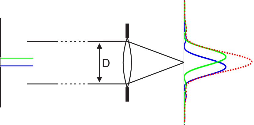
Figure 1: A one dimensional double star (two delta peaks on the left) gets imaged by the lens with the finite aperture leading to an blurred image formed by the sum of two squared sinc functions on the right.

Fig. 1 illustrates a typical experimental setup: two point sources (in green and blue on the left) are imaged through an optical system consisting here of a single lens (with focal length $f$) and a finite aperture of diameter $D$. Under incoherent illumination the observed image on the right is a superposition of the images of the point sources, each of which is given by the impulse response of the optical system $\Psi$. In an ideal diffraction-limited optical system, two point sources can only be resolved if they are at least $1.22\lambda f/D$ apart. To demonstrate that we can resolve beyond this so-called Rayleigh limit, we place the two point sources so close, that their individual images cannot be resolved (i.e. the red dashed line in Fig. 1 has only one maximum).

4.1 Recovering a one-dimensional simulated image

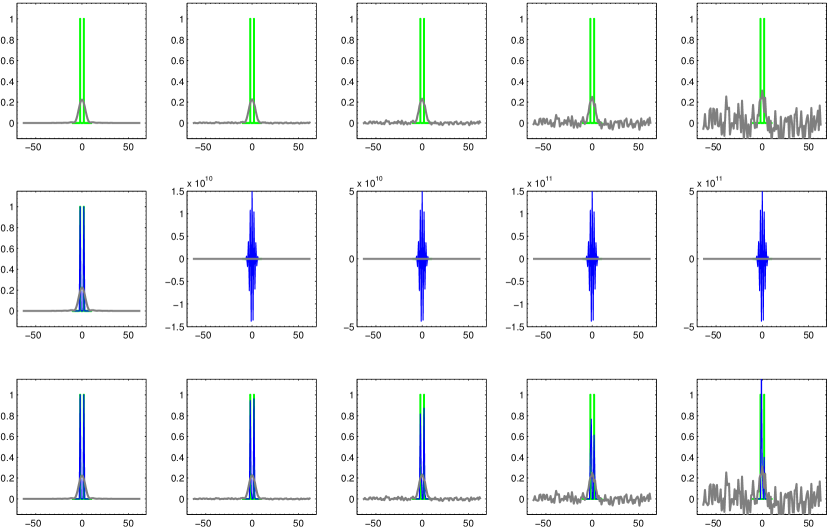
Figure 2: Restoring a diffraction-limited image (gray, first row) of one-dimensional double star (green, first row) with increasing amounts of noise (from left to right). The maximum likelihood solution (blue, second row) restores the double stars only in the noise-free cases (left column). The non-negatively constrained maximum likelihood approach (blue, third row) restores the double star even for various amounts of noise (third row, left to right).

The recorded image is usually corrupted by measurement noise, sometimes modeled as additive Gaussian. Then Eq. (26) becomes $q(.)=\mu(P)+n$ where $n\propto N(0,\sigma)$. The first row of Fig. 2 shows the true object (green) and the observed image (gray) of a one dimensional toy example for increasing amounts of noise (from left to right). More precisely, we represent the true object $p$ and the recorded image $q$ as finite-length one-dimensional column vectors $u$ and $v$. According to the Fraunhofer diffraction equation, the relationship between the object $u$ and image $v$ is linear and can be expressed as a matrix:

$$v=F^{\mathsf{H}}TFZu+n.$$ (32)

Here, $Z$ is a zero-padding matrix, $F$ is the discrete Fourier transform matrix, $F^{\mathsf{H}}$ the hermitian matrix of $F$ (i.e. the inverse transform), and $T$ is the optical transfer function (OTF), i.e. the Fourier transform of the system’s impulse response, i.e. $T=F\psi$, with $\psi$ being a finite dimensional vector, too.

The object $u$ can be recovered from $v$ by a maximum likelihood approach, i.e. we solve the following least-squares problem

$$\text{min}_{u}\|v-F^{\mathsf{H}}TFZu\|^{2}.$$ (33)

The middle row of Fig. 2 shows the recovered objects $u$ of the noisy observations $v$ (first row in gray) using the Matlab command

                       u = (F’*T*F*Z) \ v;

As suggested by our findings in Section 3, the true signal can be recovered exactly in the noise-free case (first column). The assumption of bounded support is implicit by chosing $u$ to be shorter than $v$. However, already small amounts of noise render the optimisation problem in Eq. (33) ill-conditioned yielding an unstable solution.

As an image accounts for the amount of recorded photons we can employ non-negativity as an additional physical constraint. Hence, instead of Eq. (33) we solve the constrained optimization problem

$$\text{min}_{u}\|v-F^{\mathsf{H}}TFZu\|^{2}\text{ s.t. }u\geq 0.$$ (34)

The non-negativity constraint stabilizes the restoration process and yields good results even for large amounts of noise (bottom row in Fig. 2). We solve the non-negative least squares problem using the Matlab command:

                   u = lsqnonneg(F’*T*F*Z, v);

4.2 Recovering a two-dimensional real image

We build an experimental setup with an artificial double star (lighted by green light) that is imaged by a cooled camera (PCO.2000) in about one meter distance. The optics of the camera consists of a changeable aperture and a single lens ($f=100$mm). Panel (d) of Fig. 3 shows a “ground truth” image that has been taken with an aperture of $4$mm and exposure time of $3$ms. Panel (a) shows the same double star but with aperture $0.5$mm. The aperture has been chosen that the angular separation of the double star is 50 percent below the Rayleigh limit. Note that the two stars are not visible anymore and the light has been spread out due to diffraction. To get a good measurement we had to expose for $4000$ms. Both images, (a) and (d), are the result of averaging eight images minus an averaged dark frame to reduce the noise to a minimum. The support is chosen by thresholding the measured image, panel (a). Applying the method described in the previous paragraph to the image in panel (a), we are able to recover the two double stars which are quite similar to the ground truth (panels (c) and (d) in Fig. 3). Note that the ground truth is more blurry since it is also photographed with a finite aperture.

(a) $v$, aperture=0.5mm	(b) $D^{\mathsf{H}}TDZu$
(c) $u$, recovered image	(d) ground truth, aperture=4mm

Figure 3: Real photograph of an artifical double star, that is clearly visible if the aperture is open (d), but not for small aperture (a). The recovered image (c) shows the two stars without blur, (b) shows the result of passing (c) through the forward model. All images show crops (size $60\times 50$) of larger images (size $647\times 570$).

5 Related work

The question whether it is possible to break the diffraction limit has been the subject of numerous works:

In 1952, Toraldo di Francia [4] stated that “we notice that the classical limit of $1.22\lambda/D$, which has always been accepted as a theoretical limit, proves instead to be only a practical limit.” Motivated by “super-gain antennas” he studies the diffraction patterns of “super-resolving pupils” which consists of concentric rings instead of a uniform pupil. He observes that for an increasing number of rings the central disc of the airy disc becomes smaller and more isolated, hereby increasing the resolution. In [5], the same author discusses the problem of resolving power from the point of view of information theory. He makes the point that several objects can lead to the same image, so without an “infinite” amount of prior information we cannot do two-point resolution.

A few years later, Wolter showed in [31] that bounded illumination (cf. our bounded support assumption on the object), is sufficient to recover higher frequencies, since the Fourier transform of a bounded object is analytic. He uses accelerating summation techniques to analytically continue the spectrum that has been cut off by an aperture. Independently of Wolter, Harris [13] also considered bounded objects and the fact that their Fourier transforms are analytic. He also proposed a method for analytic continuation (for the noise-free case). His conclusion is that “diffraction imposes a resolution limit which is determined by the noise of the system rather than by some absolute criterion.”

Barnes [1] proposed a reconstruction procedure for coherent illumination. He uses the assumption of bounded support to write the convolution operator in the imaging equation in such a way that it can be decomposed into prolate spheroidal wave functions [27]. This allows inversion of that operator, similar to division in Fourier space. Rushforth and Harris [22] study the influence of noise on reconstruction methods to overcome the diffraction limit. Their conclusion is that “the Rayleigh criterion is an approximate measure of the resolution which can be achieved easily.”

Gerchberg [8] (and independently Papoulis [19]) proposed an algorithm analogous to Gerchberg and Saxton’s phase retrieval method [9] incorporating also positivity. As Jones [18] points out, this algorithms converges under certain conditions only rather slowly.

Although the above works have provided insight into theoretical aspects of recovering object properties beyond the diffraction limit, the proposed methods did not become relevant in practice. In 1993, Sementilli, Hunt and Nadar [26] derived bounds on the bandwidth extension in terms of object size and noise variance under the assumption of bounded object support and positivity. Section 6.6 of Goodman’s book on Fourier Optics [10] discusses these early studies of the diffraction limits and concludes, that “the Rayleigh limit to resolution represents a practical limit to the resolution that can be achieved with a conventional imaging system.”

Several papers consider a bounded support constraint to overcome the diffraction limit. Another possible constraint is sparsity: Donoho [6] studied the problem of recovering a sparse signal for which only low frequencies of its Fourier transform are available. Recently, Candes and Fernandez-Granda [3] also studied conditions under which sparse signals can be recovered. The results apply to signals which have a sparse representation. Sparsity has effectively also been practically used to break the diffraction limit using hardware, e.g. in stimulated emission depletion microscopy (STED) [14].

Finally, one should mention that the works above consider superresolution as the problem of breaking the diffraction limit, as opposed to trying to “only” increase the resolution of low resolution sensors (e.g. [17]). This type of superresolution is not the topic of this paper so we refer the reader to the review of Park, Park and Kang [20].

6 Conclusion

We have developed a novel connection between machine learning and Fourier optics, identifying a positive definite kernel with the squared Fourier transform of an imaging system’s aperture. Leveraging results from RKHS theory, this led to a condition on an object (boundedness of its support) which ensures that it can be fully reconstructed from the image. Simple experiments showed that such reconstructions are possible with real data. While we do not claim that our approach has immediate practical implications, we believe it is surprising and noteworthy that a celebrated results in Fourier optics can be analyzed using the theory of positive definite kernels used in machine learning, with nontrivial implications for the profound problem of optical super-resolution. We hope this link can be further exploited to gain a beter understanding and possibly novel solutions to optical problems. In an experimental setup we show that we are able to super-resolve beyond the Rayleigh limit.

References

- [1] C.W. Barnes. Object restoration in a diffraction-limited imaging system. Journal of the Optical Society of America, 56(5):575–578, May 1966.
- [2] K.R. Barnes. The Optical Transfer Function. Hilger, London, 1971.
- [3] E. Candes and C. Fernandez-Granda. Towards a mathematical theory of super-resolution. Arxiv preprint arXiv:1203.5871, 2012.
- [4] G. Toraldo di Francia. Super-gain antennas and optical resolving power. Il Nuovo Cimento (1943-1954), 9:426–438, 1952.
- [5] G. Toraldo di Francia. Resolving power and information. Journal of the Optical Society of America, 45(7):497–501, 1955.
- [6] D.L. Donoho. Super-resolution via sparsity constraints. Technical Report 285, Department of Statistics, University of California, Berkeley, January 1991.
- [7] K. Fukumizu, A. Gretton, X. Sun, and B. Schölkopf. Kernel measures of conditional dependence. In J.C. Platt, D. Koller, Y. Singer, and S. Roweis, editors, Advances in Neural Information Processing Systems, volume 20, pages 489–496, Cambridge, MA, USA, 09 2008. MIT Press.
- [8] R.W. Gerchberg. Super-resolution through error energy reduction. Optica Acta, 21(9):709–720, 1974.
- [9] R.W. Gerchberg and W.O. Saxton. A practical algorithm for the determination of phase from image and diffraction plane images. Optik (Stuttgart), 35:225–246, 1972.
- [10] J.W. Goodman. Introduction to Fourier Optics. McGraw-Hill, second edition, 1996.
- [11] A. Gretton, K.M. Borgwardt, M. Rasch, B. Schölkopf, and A.J. Smola. A kernel method for the two-sample-problem. In B. Schölkopf, J. Platt, and T. Hofmann, editors, Advances in Neural Information Processing Systems, volume 19, pages 513–520, Cambridge, MA, USA, 09 2007. MIT Press.
- [12] A. Gretton, K. Fukumizu, C.H. Teo, L. Song, B. Schölkopf, and A.J. Smola. A kernel statistical test of independence. In J.C. Platt, D. Koller, Y. Singer, and S. Roweis, editors, Advances in Neural Information Processing Systems, volume 20, pages 585–592, Cambridge, MA, USA, 09 2008. MIT Press.
- [13] J.L. Harris. Diffraction and resolving power. Journal of the Opt. Soc. of America, 54(7):931–946, 1964.
- [14] S.W. Hell and J. Wichmann. Breaking the diffraction resolution limit by stimulated emission: stimulated-emission-depletion fluorescence microscopy. Optics letters, 19(11):780–782, 1994.
- [15] M. Hirsch. Blind Deconvolution in Scientific Imaging & Computational Photography. PhD thesis, University of Tübingen, 2011.
- [16] T. Hofmann, B. Schölkopf, and A.J. Smola. Kernel methods in machine learning. Annals of Statistics, 36(3):1171–1220, 06 2008.
- [17] M. Irani and S. Peleg. Super resolution from image sequences. In Proceedings of the 10th International Conference on Pattern Recognition, pages 115–120, 1990.
- [18] M. Jones. The discrete Gerchberg algorithm. Acoustics, Speech and Signal Processing, IEEE Transactions on, 34(3):624–626, 1986.
- [19] A. Papoulis. A new algorithm in spectral analysis and band-limited extrapolation. IEEE Transactions on Circuits and Systems, CAS-22(9):735–742, September 1975.
- [20] S.C. Park, M.K. Park, and M.G. Kang. Super-resolution image reconstruction: a technical overview. Signal Processing Magazine, IEEE, 20(3):21–36, 2003.
- [21] W. Rudin. Functional Analysis. McGraw-Hill, 1991.
- [22] C.K. Rushforth and R.W. Harris. Restoration, resolution, and noise. Journal of the Optical Society of America, 58(4):539–545, April 1968.
- [23] B.E.A. Saleh, M.C. Teich, and B.E. Saleh. Fundamentals of photonics, volume 22. Wiley, 1991.
- [24] B. Schölkopf and A.J. Smola. Learning with Kernels. MIT Press, Cambridge, MA, USA, 2002.
- [25] B Schölkopf, BK Sriperumbudur, A Gretton, and K Fukumizu. RKHS representation of measures applied to homogeneity, independence, and Fourier optics. Technical Report pp. 42–44, OWR 30/2008, Mathematisches Forschungsinstitut Oberwolfach, 2008.
- [26] P.J. Sementilli, B.R. Hunt, and M.S. Nadar. Analysis of the limit to superresolution. Journal of the Optical Society of America A, 10(11):2265–2276, 1993.
- [27] D. Slepian, H.O. Pollak, and H.J. Landau. Prolate spheroidal wave functions. Bell System Technical Journal, 40:43–84, January 1961.
- [28] A. Smola, A. Gretton, L. Song, and B. Schölkopf. A Hilbert space embedding for distributions. In Proc. 18th International Conference on Algorithmic Learning Theory, pages 13–31. Springer-Verlag, 2007.
- [29] B. K. Sriperumbudur, A. Gretton, K. Fukumizu, B. Schölkopf, and G. Lanckriet. Hilbert space embeddings and metrics on probability measures. Journal of Machine Learning Research, 11:1517–1561, 2010.
- [30] H. Wendland. Scattered data approximation. Cambridge Univ Pr, 2005.
- [31] H. Wolter. Verfahren zur beliebig genauen Berechnung einer Originalnachricht aus endlich vielen Beobachtungen hinter einem Rechteckbandpaß. Archiv der Elektrischen Übertragung (A.E.Ü.), 13(9):393–404, 1959.