Structure and magnetism of disordered carbon

Abstract

Motivated by the observation of ferromagnetism in carbon foams, a massive search for (meta)stable disorder structures of elemental carbon is performed by a generate and test approach. We use the Density Functional based program SIESTA to optimize the structures and calculate the electronic spectra and spin densities. About 1% of the 24000 optimized structures presents magnetic moments, a necessary but not sufficient condition for intrinsic magnetic order. We analyze the results using elements of graph theory. Although the relation between structure and the occurrence of magnetic moments is not yet fully clarified, we give some minimal requirements for this possibility, such as the existence of three-fold coordinated atoms surrounded by four-fold coordinated atoms. We discuss in detail the most promising structures.

I Introduction

Carbon has many ordered allotropes but also interesting amorphous structures. As a result of particular growth mechanisms it is found also in disordered porous structures formed by interconnected nanometer sized clusters, often called nanofoams. This type of structures have been imaged in Transmission Electron Microscope (TEM) experiments Rode1999 ; Rode2002 . Carbon nanofoams are obtained by high-repetition-rate laser ablation of a glassy carbon target in an ambient non-reactive Ar atmosphere. Scanning Tunneling Microscopy (STM) reveals a mixed $sp^{2}$ $sp^{3}$ bonding and curved graphite-like sheets. The Fourier Transform of STM images reveals clusters arranged with period of 5.6 Å  Rode1999 ; Rode2002 ; Rode2004 .

A reason of interest for these structures is the presence of ferromagnetic behaviour up to 90 K reported in Ref. Rode2004 which raises questions about the mechanism for this phenomenon. These disordered structures might present magnetic moments related to undercoordinated atoms or to particular atomic arrangements. The purpose of this work is to investigate, by means of a large number of realizations of nanosized clusters, if some atomic arrangements appear recurrently and can give rise to magnetic moments and/or to magnetic order.Our analysis provides minimal criteria for the occurrence of magnetic moments and proposes several structures of defected carbon that might present ferromagnetic order.

We first describe in section II the procedure to generate and relax in an automated fashion, series of disordered samples and the criteria to analyse this large set of results (about 24300 realizations) according to total energy, coordination and magnetic moments. In our search we consider cluster structures periodically repeated to form a bulk. In this way we disregard the possibility of magnetism related to the surfaces.

In section III we present a first screening of the magnetic properties that are the focus of our study.

In section IV we examine the distribution of total energy, some structural properties and try to establish a kind of phase diagram to relate the presence of sizeable magnetic moments to the total energy of the structure.

In section V we set up a model, based on the graph theory to analyse the networks of bonds around a magnetic atom. This model has been used to analyse the allotropes of $C_{60}$ in a famous paper by Wales c60-funnel revealing a distribution of energy with many deep minima separated by high barriers forming a funnel with minimum energy corresponding to the icosahedral $C_{60}$. Furthermore the graph theory can be related to the concept of bipartite lattices that play an important role in graphene. Also in our search we find that carbon can form a wealth of metastable disordered structures with not a high penalty in terms of energy. We aim at finding the reason why some of these realizations carry magnetic moments and may even lead to ferromagnetic behaviour.

In section VI we single out only the structures with sizeable magnetic moments and analyse them in the spirit of the mean field approximation in terms of exchange energies. Most magnetic structures have antiferromagnetic order but a few of them present a hint of ferri- or ferromagnetic order. Unfortunately the LDA-CA and GGA-PBE approximations often do not agree in the evaluation of total energy and give small variations in bond lengths. Nevertheless we show that besides these disagreements result obtained in both model are qualitatively consistent.

In the last section VII we focus on the most interesting samples found in our search and try to establish some recurrent features and minimal requirements for the presence of magnetic order.

Our search and analysis is certainly not exhaustive and many questions remain open but it represents a first systematic attempt to grasp the physics and bonding leading to ferri/ferromagnetism in disordered carbon structures. We also giveac-xsf-data the structure and coordinates of the selected samples presented in section VII in the xsf file format suitable for use in the VESTA program vesta .

II Procedure for the generation of disordered samples

In this section we describe how we generate nanosized disordered samples, relax them to find (meta)stable structures and then calculate their magnetic properties. We calculate electronic and magnetic structures within the DFT DFT-1 ; DFT-2 by means of the SIESTA code which implements DFT on a localized basis set SIESTA-1 ; SIESTA-2 ; SIESTA-3 . We used LDA with Ceperly and Alder parametrization (LDA-CA) LDA-CA-1 ; LDA-CA-2 and a standard built-in double-$\zeta$ polarized (DZP) DZP-NAO basis set to perform geometry relaxation. For some cases we used also the Generalized Gradient Approximation with Perdew-Burke-Ernzerhof exchange model (GGA-PBE) GGA-PBE . In general, the GGA gives much more accurate results for cohesive energy, equilibrium structure and related characteristics of molecules and crystals. Neither LDA nor GGA, however, can take into account van der Waals interactions which are crucially important to describe the interlayer binding in graphite. As a result, GGA without van der Waals interaction cannot describe the stability of graphite Rydberg2003-vdw-dft whereas, by chance, due to error cancellation, LDA gives a relatively accurate interlayer distance and binding energy in graphite. Therefore, it is now common practice to use the LDA for calculation of multilayer graphitic systems (see e.g. Boukhvalov-bl-graphene and references therein). The price to pay for this choice is that diamond becomes slighlty more energetically favourable than graphite (see Fig.2) contrary to experiment. We do not think that this shortcoming is important for our results.

The DZP basis set represents core electrons by norm-conserving Troullier-Martins pseudopotentials pseudopotentials in the Kleynman-Bylander nonlocal form nonlocal-form . For a carbon atom this basis set has 13 atomic orbitals: a double-$\zeta$ for 2s and 2p valence orbitals and a single-$\zeta$ set of five d orbitals. The cutoff radii of the atomic orbitals were obtained from an energy shift equal to 0.02 Ry which gives a cut-off radius of 2.22 Š for s orbitals and 2.58 Š for p orbitals. The real-space grid is equivalent to a plane-wave cutoff energy of 400 Ry, yielding $\approx$ 0.08 Š resolution for the sampling of real space. We used k-point sampling of the Brillouin zone based on the Monkhorst-Pack scheme Monkhorst-Pack with 32 k-points. An iterative conjugate gradient (CG) procedure is then applied to reach stable or metastable structures. The geometries were relaxed until all interatomic forces were smaller than 0.04 eV/Š and the total stress less than 0.0005 eV/ų. No geometrical constrains were applied during relaxation. It is important to notice that, due to the random nature of the samples, many of them have to be metastable also after the CG minimization and could evolve after annealing by molecular dynamics to energetically more favourable structure and change their magnetic property.

To construct structures similar to those observed experimentally Rode1999 ; Rode2002 , we generated samples with a given number of atoms from 5 to 64 in periodically repeated unit cells with size 5-10 Å. To simulate the experimental conditions of high pressure we used geometries compressed up to 45% of their equilibrium size. According to our calculations by DFT with the SIESTA code the initial structures have an internal pressure of 200-600 GPa.

To compensate the high internal stress, the CG relaxation leads to drastic changes of the initial structure. In this way, the minimization procedure gives a chance to reach high energy metastable configurations with the possible presence of magnetic states, similar to the situation observed experimentally for carbon nanofoams.

Table 1: Number of magnetic samples with total (absolute) spin polarization $m$ ($m_{abs}$) calculated using equations (3) corresponding to a set of magnetization intervals in $\mu_{B}$.

$N_{atoms}$	$N_{samples}$	$m(m_{abs})>0.01$	$>0.05$	$>0.10$	$>0.25$	$>0.5$	$>1.0$
5	1000	22(23)	22(23)	21(22)	2(2)	2(2)	0(0)
6	1000	0(0)	0(0)	0(0)	0(0)	0(0)	0(0)
7	1000	26(26)	26(26)	26(26)	14(14)	14(14)	0(0)
8	10000	7(7)	3(7)	3(4)	1(2)	0(1)	0(1)
9	1000	7(9)	7(7)	6(6)	3(3)	3(3)	0(0)
10	4000	27(27)	27(27)	26(26)	22(23)	16(18)	0(0)
11	1000	6(6)	6(6)	6(6)	5(5)	3(3)	0(0)
12	1000	14(15)	13(14)	12(13)	9(11)	3(7)	0(2)
13	1000	11(13)	10(11)	10(11)	8(9)	6(7)	1(3)
14	1000	15(15)	13(14)	12(14)	11(13)	7(12)	0(2)
15	1000	16(16)	15(16)	14(16)	12(15)	10(15)	1(2)
16	1100	28(28)	24(28)	22(27)	18(25)	13(21)	0(5)
24	100	4(4)	4(4)	4(4)	4(4)	3(4)	0(0)
64	100	5(13)	3(9)	3(8)	3(8)	3(8)	3(8)

To generate the initial geometries we used the following approach. First of all, we calculate the volume per atom in the graphite unit cell:

$$v^{graphite}_{atom}=\frac{3\sqrt{3}}{4}r_{cc}^{2}r_{ll}$$ (1)

where $r_{cc}=1.42$ Å  is the carbon-carbon interatomic distance in the layer and $r_{ll}=3.35$ Å  is the interlayer distance in graphite. Since we will construct compressed unit cells by scaling of the coordinates, it is convenient to express $r_{ll}$ in terms of $r_{cc}$. For graphite $r_{ll}=2.36~{}r_{cc}$. In this way, the volume $v^{graphite}_{atom}$ can be written as proportional to $r_{cc}^{3}$ and $\sqrt[3]{v^{graphite}_{atom}}$ becomes proportional to $r_{cc}$. Rescaling the unit cell size by $r_{cc}^{custom}$ we can construct the initial cubic unit cell for a given number of atoms $N_{atoms}=n$ with lattice constant $a$ as

$$a=\frac{\sqrt[3]{nv^{graphite}_{atom}}}{r_{cc}}r_{cc}^{custom}$$ (2)

To allocate the required number of atoms within the prepared cubic unit cell we randomly generated atomic coordinates. If the newly generated position is closer than $r_{cc}^{custom}$ to any atom we replaced such a pair by one atom with average position. At the end, the geometry has no atoms closer than $r_{cc}^{custom}$. For the case $r_{cc}^{custom}$ = 1.42 Å  the density of the generated system is equal to the one of graphite. We used $r_{cc}^{custom}$ = 1.1 Å  that gives a density $\approx$2.15 higher than graphite.

Table 2: An overview of the obtained information about coordination in all studied configurations. The percentage of samples with specific coordination is shown for each series of atoms. Since the case of 6 3-fold atoms is not applicable to the series with 5 atoms and it duplicates the value of all 3-folds configurations for the series with 6 atoms we keep these two cells empty.

$N_{atoms}$	$N_{samples}$	all 3-fold	2 3-fold	4 3-fold	6 3-fold	all 4-fold	1 2-fold	2 2-fold	3 2-fold
5	1000	0.0	15.4	38.1	-	46.4	17.8	0.0	1.3
6	1000	33.2	32.4	25.0	-	9.3	7.3	4.9	0.0
7	1000	0.0	30.8	19.1	32.2	17.3	8.1	0.2	0.0
8	10000	22.7	22.0	23.6	9.0	22.4	1.5	0.4	0.0
9	1000	0.0	25.6	31.3	14.3	17.2	1.8	0.1	0.0
10	4000	10.2	22.5	22.5	24.1	11.3	2.5	0.6	0.05
11	1000	0.0	23.0	29.6	19.9	12.8	3.2	0.5	0.2
12	1000	4.6	21.1	24.7	16.7	12.8	1.8	0.3	0.0
13	1000	0.0	24.1	24.1	19.5	7.1	3.0	0.5	0.0
14	1000	2.0	17.3	21.8	23.9	6.5	2.6	0.4	0.0
15	1000	0.0	18.0	21.6	22.8	6.5	4.5	1.3	0.0
16	1100	1.2	16.3	21.5	20.7	7.5	4.5	0.3	0.2
24	100	0.0	4.0	11.0	21.0	0.0	6.0	3.0	0.0
64	100	0.0	0.0	0.0	0.0	0.0	11.0	4.0	1.0

Such a randomly generated geometry with high internal pressure and fixed number of atoms per unit cell is then minimized by CG letting the atomic positions within the cell and the cell lattice parameters vary. We then study each sample to search for magnetic states in pure carbon materials. We have studied in this way 24300 samples. A first screening gives $\approx$1% (see Table 1) of the samples with magnetic states. In Table 2 we report the coordination in samples with 5 to 64 atoms in the unit cell, calculated automatically by counting the number of neighbors closer than 1.8 Å.

In the following we use the following notation to refer to a specific sample, namely ACxx-yyyy where AC stays for amorphous carbon, xx is the number of atoms in the unit cell and yyyy denotes a specific sample. As an example, the sample AC07-0010 shown in Fig. 8 is the tenth of a series with 7 atoms in the unit cell.

We see that also samples with only 3-fold or 4-fold bonding are found. Their number decreases for the larger unit cells as expected because there are many more possible configurations. We find, as expected from considerations that will be discussed in section V, no samples with all 3-fold atoms for odd $N_{atoms}$. Unexpected is that for $N_{atoms}=8$ there is a maximum number of all 4-fold samples. For the samples with mixed bonding we report the percentage of samples with 2, 4 or 6 3-fold bonded atoms. In general the 4-fold atoms have bonding angles very close to that of $sp^{3}$ hybridization in diamond and very often 3-fold atoms are almost flat $sp^{2}$ configurations like in graphitic forms of carbon. Within the many possible configurations, we distinguish those with all 3-fold atoms (graphite-like $sp^{2}$ structure), all 4-fold atoms (diamond-like $sp^{3}$ structure), configurations with 2-fold coordinated atoms and mixed configurations with different percentage of 3-fold and 4-fold atoms. The two first groups (all 3-fold and all 4-fold) are non magnetic and the last two groups are possible candidates for magnetic states as it will be discussed in more details in section V.

To distinguish between ferromagnetic and antiferromagnetic samples we use the total spin polarization $m$ and the total absolute spin polarization $m_{abs}$

$$m=\sum_{i=1}^{N_{Atoms}}s_{i},~{}~{}~{}~{}m_{abs}=\sum_{i=1}^{N_{Atoms}}|s_{i}|,$$ (3)

$$s_{i}=q_{i}^{up}-q_{i}^{down}$$ (4)

where $q_{i}^{up}$ is the charge corresponding to spin ”up” at the i-th atoms and $q_{i}^{down}$ is the charge corresponding to spin ”down” at the i-th atoms.

We can then distinguish antiferromagnetic samples, where $m=0$ and $m_{abs}\neq 0$, and ferromagnetic ones for which $m=m_{abs}$. Moreover we found a set of samples where $m>0$ and $m\neq m_{abs}$. This is a sign of ferrimagnetic properties.

III Search of magnetic states

To identify the geometrical structures responsible for the magnetic states, we perform a numerical experiment based on a generate and test approach generate-test with elements of genetic algorithms genetic-algorithm . Such a method is convenient in view of the available large amount of computational facilities which allows to calculate automatically thousands of independent configurations. We varied the number of atoms together with the unit cell size and number of configurations in the computational series iteratively to identify the most typical geometrical structures carrying magnetic states.

We started with 64 atoms per sample and 100 samples in the series. We found 5 configurations with total spin polarization $m>0.010\mu_{B}$ and only 3 with $m>0.500\mu_{B}$, (see Table 1 last row). At the same time, from Table 1, we see that within the series with 64 atoms besides the samples with sizeable total spin polarization $m$ there are a number of samples (i.e. 8-3=5 samples) where $m$ is small while $m_{abs}$ is of the order of $\mu_{B}$. This facts is a clear evidence of antiferromagnetic arrangement of magnetic moments in the ground state as discussed at the end of section II.

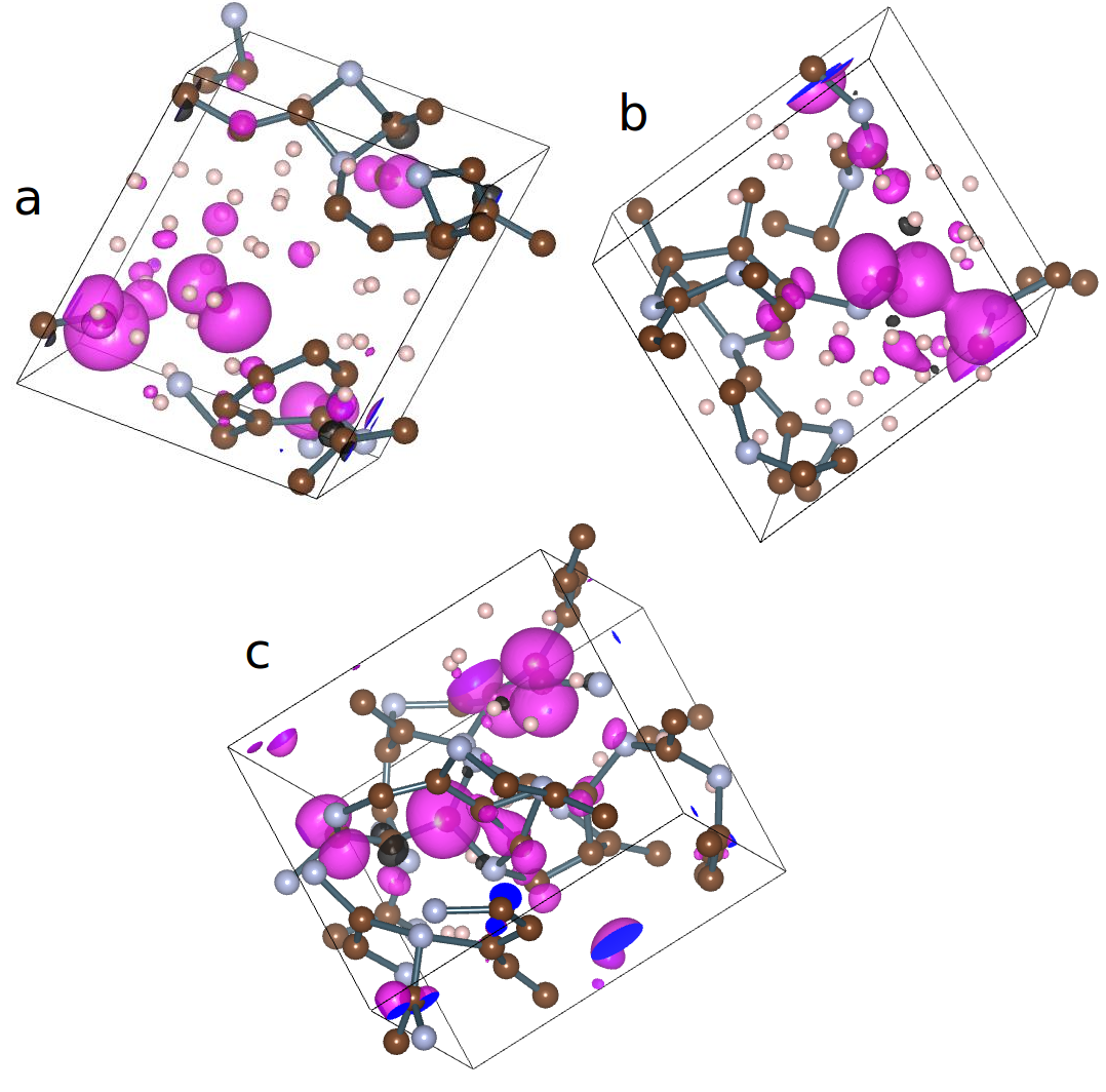
Figure 1: Examples of spin polarized structures for disordered carbon (64 atoms per unit cell) after relaxation, showing atoms with magnetic states (pink clouds) surrounded by nonmagnetic ones. The 4-fold atoms are small balls marked by light gray, the 3-fold atoms are balls marked by brown. The 4-fold with 3-fold neighbours are balls marked by gray. The 1D chains of 3-fold atoms separated by single 4-fold atoms are marked by bonds. Here we see well distinguishable networks made of 1D chains of 3-fold atoms. We see that not all the magnetic atoms belong to these chains. The geometry is visualized by the VESTA program vesta .

A first analysis shows that magnetic moments are carried by individual atoms in specific atomic configurations. Typical configurations with magnetic atoms are shown in Fig. 1a,b,c. We have highlighted the presence of networks of 3-fold atoms. We will come back to the relation between these networks and the magnetic atoms in section V.

One might have expected the source of uncompensated spin to be dangling bonds originating from 2-fold carbon atoms as it was shown for grain boundaries in DBGB . We find instead that also 3-fold carbon atoms may have uncompensated spin and that this latter case occurs at least one order of magnitude more frequently than 2-fold atoms. While for 2-fold coordinated atoms the magnetic moment is clearly related to a dangling bond, the situation of 3-fold coordinated atoms is more complex. Depending on the bond angles, it may correspond to a planar $sp^{2}$ configuration like in graphite or to a $sp^{3}$ configuration with a dangling bond as found for instance at the ideal (111) diamond surfaces.

Within the first series of samples with 64 atoms we have shown that only 3 configurations have more than one magnetic atom. This suggests that probably the geometrical conditions which make atoms magnetic can be detected in smaller and simpler geometries with fewer atoms per unit cell. To do so we iteratively reduced the number of atoms together with the unit cell size.

In the second series with 100 configuration and 24 atoms per sample we found 4 configurations with total spin polarization $m>0.005\mu_{B}$ and only 3 with $m>0.500\mu_{B}$. Typically, we had 1-2 magnetic atoms per unit cell.

In view of the small number of magnetic atoms in each sample, to make our search for structures with magnetic states more efficient we generated and optimized series of thousands of configurations with less atoms (16 to 5 atoms) per unit cell. Let us notice a few interesting facts. First of all, we did not find any magnetic configurations within 1000 samples in the series with 6 atoms per unit cell and only 3 magnetic configurations with $S>0.100\mu_{B}$ within 10000 samples in the series with 8 atoms per unit cell. The series with 5 and 7 atoms per unit cell instead presents magnetic configurations. This could be a sign of the importance of the parity of the number of atoms in the unit cell.

By reducing the number of atoms per unit cell we also reduce the number of possible relaxed configurations. This reduction is reflected in the presence of duplicate geometries up to variations in the directions of the unit cell vectors. The presence of duplicate geometries also suggests that, within the constraints imposed by the sample construction, such geometries are more preferable than the others.

IV Energy and magnetism

Table 3: Comparison of the 6 computational models used to calculate the formation energy of 5 carbon allotropes, i.e. 3 sets of parameters within GGA-PBE and 3 sets of parameters within the LDA-CA approximation. Here $E_{mesh}$ gives the resolution for the sampling of real space based on the plane-wave cutoff energy. $E_{cutoff}$ is the cutoff radius of the atomic orbitals. (see section II) Two types of basis sets were chosen: the standard DZP and the custom one constructed for graphitic materials using the approach described in DZP-NAO ; variational-approach . Notice that the minimal energy structure is graphite for GGA-PBE and diamond for LDA-CA.

GGA-PBE, 32 k-points	DZP	DZP	custom
$E_{mesh}$ = 400 Ry	$E_{cutoff}$ = 1 mRy	$E_{cutoff}$ = 20 mRy	basis
diamond	0.021	0.008	0.112
graphene	0.007	0.066	0.003
graphite-A	0.002	0.015	0.001
graphite-AB	0.000	0.001	0.000
graphite-ABC	0.001	0.000	0.001
LDA-CA, 32 k-points	DZP	DZP	graphite
$E_{mesh}$ = 400 Ry	$E_{cutoff}$ = 1 mRy	$E_{cutoff}$ = 20 mRy	basis
diamond	0.000	0.000	0.000
graphene	0.195	0.257	0.079
graphite-A	0.173	0.166	0.059
graphite-AB	0.156	0.131	0.044
graphite-ABC	0.157	0.132	0.044

Within thousands of calculated configurations with formation energy lying between 0.0 and 2.0 eV/atom above diamond, as shown in Fig. 2 a few hundreds magnetic ones were found with different energies and spin polarizations. We note that, besides diamond and graphite there is another sharp peak at low energy. Since these configurations are not magnetic we have not analysed them in detail but in a few cases we have seen that they relax to diamond or graphite after annealing. In Fig 3 we analyse the relation between formation energy and magnetic moments. The total energy per atom for magnetic configurations lies in a relatively restricted range of 0.6-1.5 eV/atom above diamond and graphite, most of them being in 0.8-1.2 eV/atom energy range. In general we cannot identify any specific energy-spin region for particular series of calculations excluding the series with 7 atoms per sample (see top polygon in Fig. 3) and partly the series with 10 atoms per sample (see middle polygon in Fig. 3). The presence of duplicates, especially for the series with 5-11 atoms that we have already discussed in III, is indicated by ellipses. Low energy configurations are indicated by rectangles and we see that they cluster in the two regions indicated by shaded polygons for energy $\leq$ 0.8 eV/atom, only 10-15 % higher than diamond and graphite.

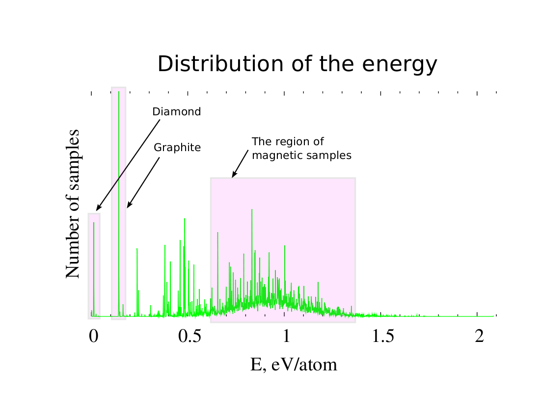
Figure 2: Distribution for the energy referred to diamond of all the calculated samples. The energy intervals marked as ”diamond” and ”graphite” corresponds to the specified systems, the third shaded energy interval contains magnetic samples and is further analysed in Fig. 3.

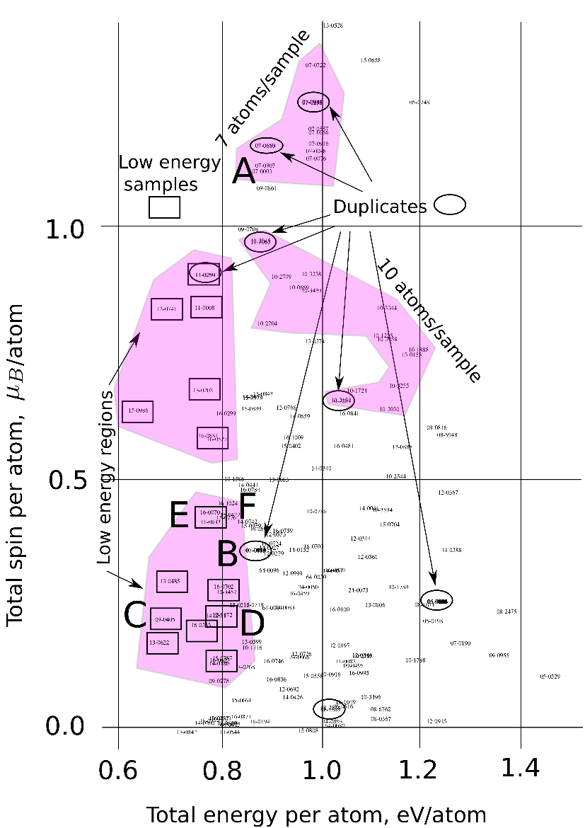
Figure 3: Total spin per atom as a function of total energy per atom (referred to diamond) for magnetic structures. Each point has a name combining the number of atoms and index in the series. Few regions of spin and energy are marked by light grey polygons. Within them, ellipses indicate the existence of many duplicates as described in the text. The two left shaded regions contain low energy structures marked by rectangles. The structures indicated as A, B, C, D are shown in Fig. 9, 8, 10 right and 10 left respectively.

The special character of the energy landscape of carbon systems, related to the fact that carbon can form a wealth of structures, often with very high energy barriers among them, has been pointed out in the seminal work c60-funnel where all the 1812 possible structures of $C_{60}$ are shown to form a funnel of well separated, deep minima not too far in energy from the absolute minimum corresponding to icosahedral $C_{60}$.

V Structure and magnetism

As we have seen in the previous section, magnetic structures are rare and the relation between structure and magnetism is certainly not trivial. We try and use the graph theory graph-theory to relate structure and magnetism. To take advantage from this theory we need to have only one odd numbered coordination. This is realized in our carbon system where no atoms with one bond or five bonds are present because such configurations are especially unstable and were never observed in our samples after geometrical relaxation.

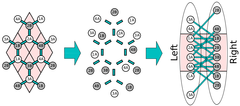
Figure 4: An example of the division procedure that maps the bipartite lattice of graphene into two disjointed subgraphs called as Left and Right. From left to right: a 2X2 supercell of graphene indicated by the light grey polygons. Atoms belonging to the A-sublattice (B-sublattice) are represented by white (grey) balls with labels 1A(B), 2A(B), 3A(B), 4A(B). Since we consider 2D periodical structure we also show the periodical images outside the unit cell. Through an intermediate step we can construct the Left and Right subgraphs as indicated by bringing all A atoms to the left and all B atoms to the right while keeping the bonds between former nearest neighbours. All the atoms originally found in the shaded (pink) unit cell are located in the shaded (pink) region of the graph.

We start by a lemma that we have derived ourselves although it might be reported already in the literature.

Lemma. Any connected graph with nodes having 2, 3 or 4 neighbours always has an even number of nodes with 3 neighbours.

Proof. Suppose we have $N_{2}$ nodes with 2 neighbours, $N_{3}$ nodes with 3 neighbours and $N_{4}$ nodes with 4 neighbours. Each edge connects two nodes. Due to this fact, the total number of edges in the graph is $(2N_{2}+3N_{3}+4N_{4})/2=M$, where $M$ is an integer positive number, whence $3N_{3}=(2M-4N_{4}-2N_{2})=2(M-2N_{4}-N_{2})$. This means that $3N_{3}$ is an even number which implies that $N_{3}$ is even.

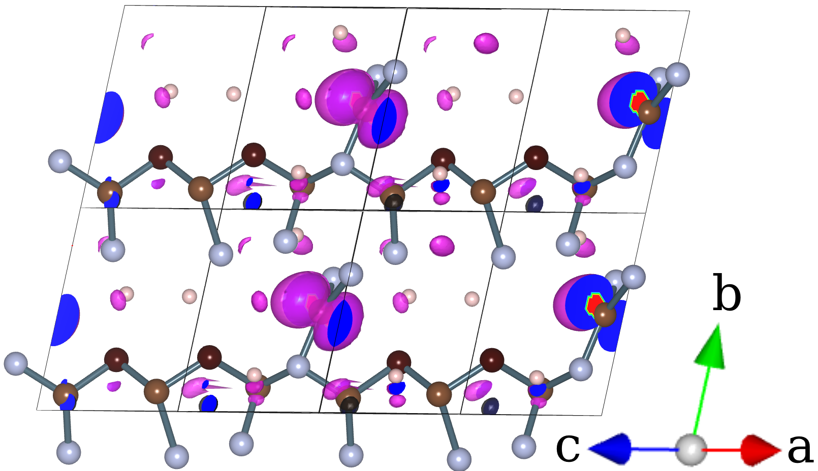
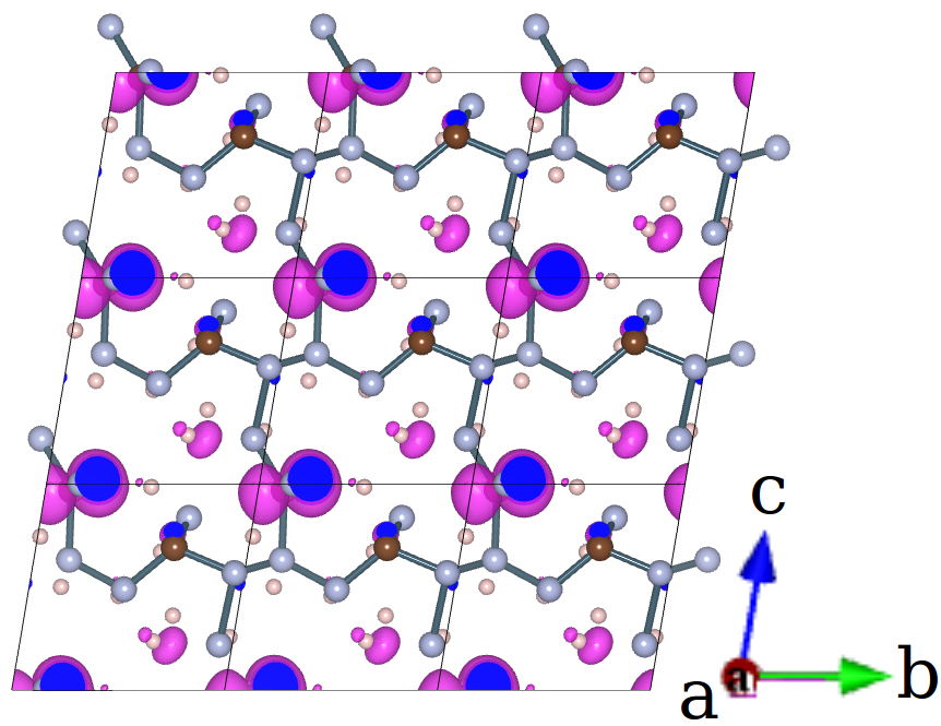
Figure 5: Examples of 1D chains (top) and 2D-networks (bottom) of connected 3-fold and 4-fold atoms. As previously (see Fig. 1) we use different colours for 3-fold and 4-fold atoms with different neighbouring atoms. The 4-fold atoms are small balls marked by light grey, the 3-fold atoms are balls marked by brown. The 4-fold having 3-fold neighbours are balls marked by grey.

The structure of the graph described in the lemma corresponds to the structure of disordered carbon where we have atoms with either 2, 3 or 4 neighbours. This case corresponds either to atoms in $sp$, $sp^{2}$ and $sp^{3}$ hybridization or atoms in $sp^{2}$ and $sp^{3}$ hybridization with dangling bonds (2 and 3 neighbours respectively).

The importance of this lemma lies, as it will be shown later, in the relation between magnetic states and the presence of atoms in $sp^{2}$ hybridization. In principle, the simplest carrier of magnetic moments are dangling bonds on 2-fold coordinated atoms. This situation however, is rather fragile because these dangling bonds give a high energy penalty and will tend to be passivated in realistic situations. For this reason we need to focus on magnetic moments associated to 3-fold coordinated atoms, which represent a substantial fraction of the cases we have found. We often observe a non compensated spin located at atoms in $sp^{2}$-hybridization with 3 neighbours and an unpaired $\pi$-orbital. Another important observation is that $sp^{2}$ atoms usually group in network structures made of 1D chains of $sp^{2}$ atoms as shown in Fig. 1. Such a structure may be represented as a bipartite graph. Graphene has a 2D bipartite unit cell Novoselov2004 . An example of a graph representation for graphene is shown in Fig. 4. According to the Lieb theorem Lieb-theorem ; Yazyev2010-report ; KatsnelsonBook we can expect the presence of nonzero spin if the number of atoms in the Left and Right subgraphs is different. According to the above lemma, we always have an even number of atoms with 3 neighbours. It turns out that in most of the studied structures this even number of 3-fold atoms is equally distributed in the Left and Right subgraphs. According to Lieb theorem in this case the ground state should be a non magnetic singlet state. As a result, to have magnetic states, we need specific geometric structures. For example, in the simplest case, the source of uncompensated spin could be a single $sp^{2}$ atom surrounded by $sp^{3}$ atoms. But, according to the lemma, we will always have at least one more $sp^{2}$ atom located somewhere in the unit cell. If these two atoms are either in different subgraphs or form a bond, no magnetic states may be expected.

One straightforward consequence of the above considerations is that the absence of 3-fold atoms in the unit cell, i.e. a fully 4-fold structure, means the absence of any magnetic states. Within 24300 optimized configurations we have 4132 fully 4-fold structures and all of them are non magnetic.

Since 3-fold atoms are the crucial ingredient to have magnetic states, we analyse our samples by evidencing the connections between 3-fold atoms. In this way we identify networks of bonds between them, as shown in Fig 1a,b,c and more in detail in Fig 5. To make the network of 3-fold atoms more evident we have marked the 4-fold atoms with tiny balls so that the remaining geometry looks like a 3D network of 1D chains of 3-fold atoms. Such a 3D network may consist of a set of isolated clusters or may form an infinite structure due to the periodic boundary conditions in any or all directions of the unit cell.

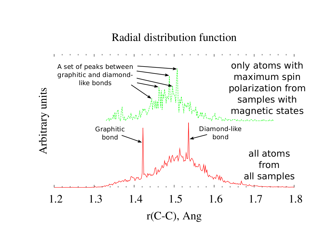
Figure 6: Comparison of the radial distribution functions calculated for all atoms of all 24300 optimized samples with that calculated by considering, for each sample with $m\neq 0$, only the atom with maximal magnetic moment.

Let us now consider one of the simplest cases where we can expect magnetic states on the basis of the lemma: two 3-fold atoms not bonded to each other within the unit cell. We can automatically detect all such configurations. Within 24300 we found 990 samples with only two 3-fold atoms not bonded to each other where 34 of them have appreciable magnetic moments in ferro- or ferri- or antiferromagnetic configurations ($m>$ 0.020 $\mu_{B}$ or $m_{abs}>$ 0.020 $\mu_{B}$). For completeness, we give the distribution of magnetic samples within each series: 8:1, 9:1, 10:6, 12:6, 13:3, 14:5, 15:4, 16:8 ($N_{atoms}$:$N_{samples}$) where 3 of them are with $m<$0.020 $\mu_{B}$ and $m_{abs}>$ 0.020 $\mu_{B}$, 20 of them are with $m\approx m_{abs}$ and other 11 with $m_{abs}>m$.

In all 34 structures the distance between the 2 3-fold atoms $>$ 2.19 Å. Since we use a localized basis set with cut-off radius of $s$ orbital 2.22 Å  (see description in section IV) we did one check with longer cut-off radius for one similar sample. For $r_{cut-off}^{2s}$ = 3.07 Å  and $r_{cut-off}^{2p}$ = 3.84 Å  we get practically the same value of $m$ for the fully relaxed geometry, ruling out the possibility of a numerical artefact. The requirement of a minimal distance of 2.19 Å  between 3-fold coordinated atoms gives 613 samples instead of 990, increasing the percentage of magnetic samples to $\approx$ 5.5%.

Within all 613 samples, we found that the 2 3-fold atoms have either 0, 1 or 2 common neighbours but we could not find any correlation between the number of common neighbours and the presence of magnetic states. We notice, however, that the presence of 2 common neighbours means that two 3-fold coordinated atoms form a tetragon. Interestingly, such a situation was found 4 times for the 34 samples with a magnetic state, a relatively high percentage.

The above analysis was performed to identify some general geometrical configurations leading to magnetism starting from the simplest possible situation. Our analysis accounts then for only 34 of the total 202 structures with magnetic moments. Nevertheless we have seen that the local environment, namely the interatomic distances and coordination of the atoms carrying a magnetic moment, plays a role. A way to further investigate this point is to compare the radial distribution function (rdf) of magnetic atoms with that of all others as we do in Fig. 6. If we average over all atoms of all 24300 studied configurations, the rdf presents two sharp peaks at the interatomic distance of graphite (1.42 Å) and diamond (1.54 Å) and a broad distribution around them from $\sim$ 1.32 Å  to $\sim$ 1.7 Å. If we consider only the atom with maximum (non-zero) magnetic moment within each sample, we find that the two sharp peaks disappear, in agreement with our discussion that rules out the possibility of magnetism for atoms with only graphitic (fully $sp^{2}$) or only diamond(fully $sp^{3}$) bonds. We see instead a number of peaks in between these two distances that have to be related to a mixed bonding. We notice that a few peaks are rather pronounced but we did not manage to assign each of them to a specific bonding configuration.

In this work we have tried to find out the most promising configurations giving rise to magnetism. As we have discussed the minimal conditions to have magnetic moments are very stringent and lead to a very small percentage of magnetic structure among the thousands studied. Nevertheless some exist and, as we show in the next section VI, could lead to magnetic order if suitably repeated. Moreover, since our analysis only gives a first insight in this phenomenon, we examine in detail in Section VII the structure of the most interesting realizations found in our quest.

VI Exchange energy

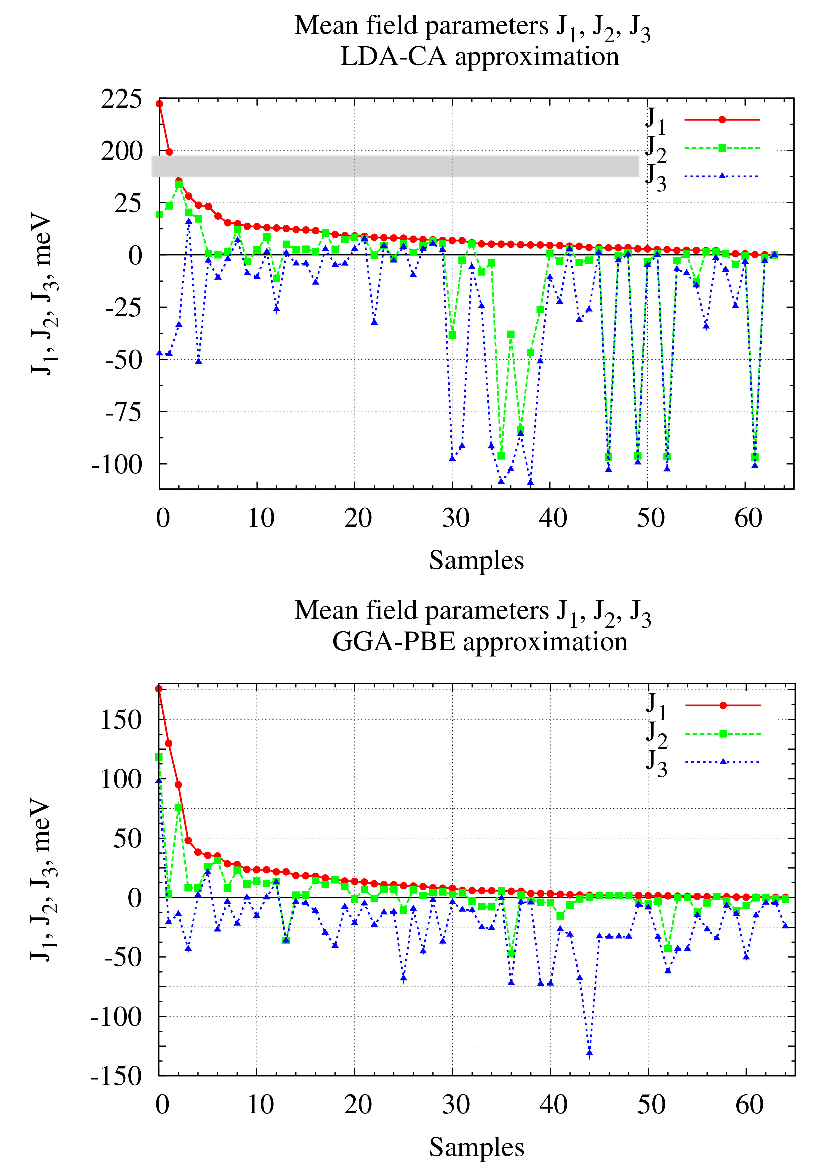
Figure 7: Mean field parameters $J_{1}$, $J_{2}$, $J_{3}$ calculated using equation (5) in 3 periodical directions sorted by the automatic procedure described in the text. Two approximations were used, i.e. LDA-CA (top panel) and GGA-PBE (bottom panel). Notice the cut in the $Y$ axis of the top panel.

In this section we focus on the samples with atoms carrying a magnetic moment and examine the possibility of magnetic order in the spirit of mean field theories.

Most of the studied samples have orthorhombic unit cells with lattice vectors $a$, $b$ and $c$ where all three periodic directions are different (i.e. anisotropic crystal). If the unit cell has only one atom with magnetic moment much larger than the others, we calculate the exchange energy $J$ for each periodic direction separately. To do so, we double the original unit cell in the chosen direction and initialize the spins on the two magnetic atoms as ”up” and ”down” in the first and second periodic images respectively and calculate the total energy which we call here $E_{AFM}$. By initializing the spins on the two magnetic atoms as ”up” and ”up” we calculate the total energy $E_{FM}$. From these two values we calculate the mean field parameters (exchange energy) as

$$J=\frac{E_{AFM}-E_{FM}}{2}$$ (5)

Since we have three independent values of $J$ calculated for unit cells doubled in the direction of the $a$, $b$ and $c$ lattice vectors, we call them here as $J_{a}$, $J_{b}$ and $J_{c}$. In order to automatize the evaluation and ordering of $J$ even though we do not have a priori any knowledge of the studied geometry we use the following procedure. We start by taking only the samples which have at least one positive value among $J_{a}$, $J_{b}$, $J_{c}$. Then, for the chosen sample, we sort the values of $J_{a}$, $J_{b}$, $J_{c}$ in descending order. The sorting breaks the relation with the $a$, $b$ and $c$ vectors so that we rename the sorted values as $J_{1}$, $J_{2}$, $J_{3}$ where $J_{1}$ is always positive and $J_{1}\geq J_{2}\geq J_{3}$. Finally we group all the chosen samples, sorting them by $J_{1}$ in descending order and make the plot shown in Fig. 7. First of all, we notice that the largest values of exchange parameters, both ferromagnetic and antiferromagnetic, can reach few hundreds meV. They correspond to magnetic atoms only a few Å  apart. Such a strong interaction for atoms near to each other is not surprising because, for example, a value of hundred meV was found for the ferromagnetic zigzag edges of graphene passivated by HydrogenLABEL:Yazyev2008-edges. In our samples that are constructed by periodically repeating relatively small cells, this situation occurs a number of times but it is hard to expect it for real carbon foam structures.

We have to note that, particularly for the large samples, and in any case in view of the large number of studied samples, we could not study the stability of the magnetic samples with respect to temperature. We could only perform the conjugated gradient optimization for the doubled cells. Both configurations with parallel and antiparallel orientation of magnetic moments were checked in this way.

The first 10 points in Fig. 7 with the highest values of $J$ in LDA-CA approximation, correspond to the following samples: AC07-0657, AC07-0680, AC07-0003, AC16-0070, AC07-0907, AC14-0388, AC14-0742, AC12-0367, AC15-0776, AC16-1024. The first 10 points in GGA-PBE approximation correspond to the samples AC14-0831, AC07-0907, AC15-0656, AC13-0119, AC15-0267, AC10-1116, AC07-0003, AC09-0394, AC07-0657, AC09-0027. Only the two samples AC07-0657 and AC07-0907 are among the first 10 in both approximations. Beside two these samples, the sample AC14-0831 has, in both approximations, a positive value of all three $J$’s. Unfortunately, as expected, the LDA-CA and GGA-PBE approximations often do not agree, especially for such a complicated case as disordered carbon where changes in the bond length up to 2-3% can dramatically change the geometry and electronic properties. In contrast to planar geometries, like the graphene grain boundaries examined in DBGB , these 3D, disordered geometries usually do not have any symmetry that can compensate small variations in the bond length. Despite these shortcomings, two samples with the highest values of $J$ are present in both approximations.

We can draw some conclusions based on our physical observations. First of all, the only few samples that have all three values of $J$ positive, making it possible to expect 3D ferromagnetism, have very small values of $J$ only up to few meV. This finding agrees with the fact that 3D ferromagnetism has been experimentally observed in carbon nanofoams only up to 90 K.

Most samples have two positive values of $J$ (see Fig. 7) making it possible to have 2D lattices of magnetic moments with ferromagnetic arrangement. In some cases the values of $J$ are rather large and might lead to high Curie temperature. Since in 2D ferromagnetic order can exist, we pay special attention to this important case. When the third value of $J$ is negative, the system has antiparallel coupling of 2D ferromagnetic networks. To exclude this effect and have only ferromagnetic couplings, we have to separate the 2D networks by imposing additional geometrical constrains. In Fig. 10 we show how this could be realized by creating 2D grain boundaries. Such a geometrical isolation of 2D structures could lead to ferromagnetic order in a bulk 3D system. In the next section VII we discuss the geometry of the most promising structures, namely those with high values of the $J$ parameters.

VII Examples of magnetic structures

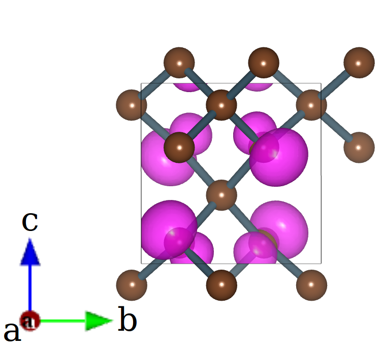
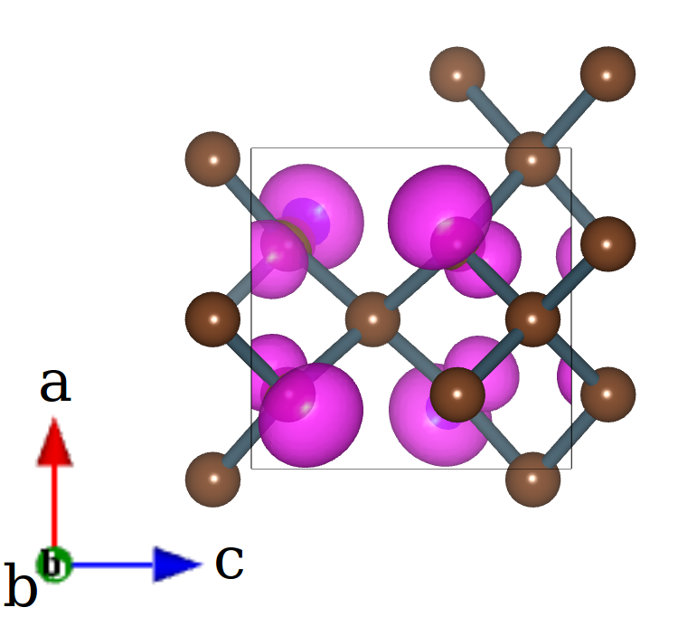
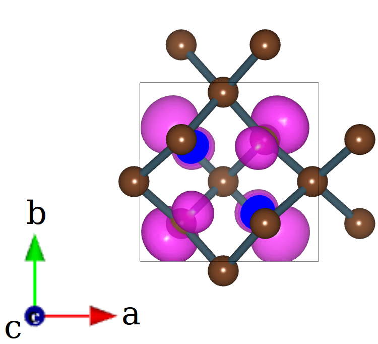
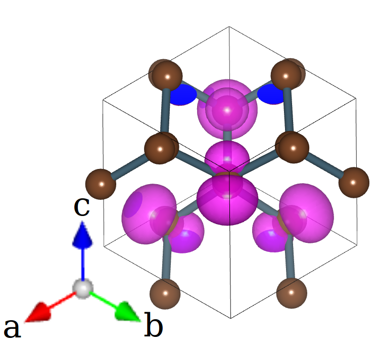
Figure 8: Spin density isosurface plot and unit cell of the sample AC07-0010 shown (from left to right, top to bottom) in the plane orthogonal to the 100, 010, 001 and 111 directions. This structure occurs 11 times in a set of 1000 samples.

Here we show a few geometrical examples discovered in our search which could be important from different points of view. Out of many and many different geometries within the series with small number of atoms, we will pay attention to the samples AC07-0003 and AC07-0010 (marked as A and B in Fig. 3). Sample AC07-0003 has high values of two $J$ parameters (see top-10 list in the text related to Fig. 7) and was found several times with small variations in geometry and sample AC07-0010 has a highly symmetric geometry with 4 $sp^{2}$ atoms with magnetic moments and appeared 11 times.

Also we will pay attention to two samples, AC09-0405 and AC14-0831 (marked as C and D in Fig. 3), due to their low formation energy (left filled region in Fig. 3, relatively simple structure, similarity to the geometry of graphite and ferromagnetic arrangement of magnetic moments.

Finally we briefly discuss two more complicated structures, AC09-0708 and AC15-0267, which have 3D ferromagnetic properties according to the GGA-PBE approximation.

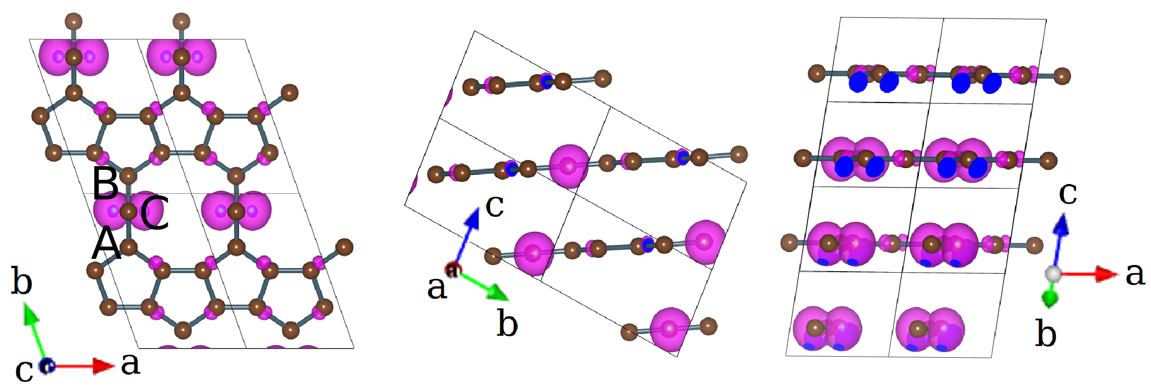
Figure 9: Spin density isosurface plot of the sample AC07-0003. Top, side and front views.

An example of a 3D bipartite unit cell is presented by the sample AC07-0010 shown in Fig. 8. Its structure can be described by considering a sequence of steps starting from a face-centred cubic cell. Taking into account all 6 atoms sitting at the centre of each face of the unit cell, we can construct an octahedron with 6 vertices and 8 faces. Within the 8 faces, we can choose 4 ones in such a way that any two of them have no common edge. Putting 4 atoms at the centre of the 4 chosen faces of the octahedron together with the original 3 atoms sitting at the faces of the cubic unit cell would finally produce our geometry. The final structure has 7 atoms where 3 of them are 4-fold coordinated in $sp^{3}$ hybridization and 4 atoms are 3-fold coordinated in $sp^{2}$ hybridization. Each of the 4 $sp^{2}$ hybridized atoms carries a magnetic moment shown as a pink cloud in Fig. 8 and contributes the value $m_{C}=0.061~{}\mu_{B}$ to the total spin polarization. The geometry has 3+4=7 atoms and (3x4+4x3)/2=12 bonds each of them of 1.51 Å, corresponding to a peak in the rdf of magnetic atoms in Fig. 6. This structure presents a frequently occurring pattern where a 3-fold coordinated carbon atom in the $sp^{2}$ hybridization is surrounded by 3 $sp^{3}$ atoms. In Fig. 4 we have seen that graphene has a 2D bipartite unit cell with one atom in the Left and one in the Right subgraphs. The sample AC07-0010 has a 3D bipartite unit cell with 4 $sp^{2}$ atoms in the Left and 3 $sp^{3}$ atoms in the Right subgraph. This situation is similar to the structure of half hydrogenated graphene hh-graphene where only the carbon atoms on one sublattice are $sp^{3}$ bonded to a hydrogen. Exactly this feature allows us to apply the Lieb theorem Lieb-theorem ; Yazyev2010-report ; KatsnelsonBook and expect non zero total spin polarization in agreement with the result of our DFT calculations.

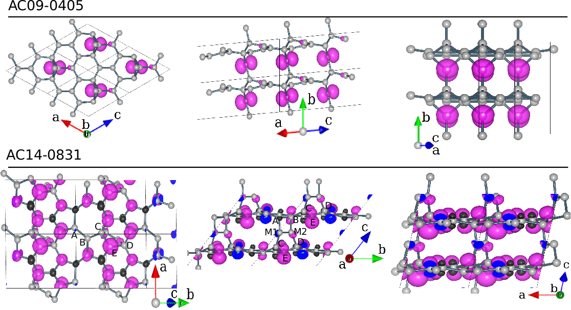
Figure 10: Spin density isosurface plot of AC09-0405 and AC14-0831 samples. For clarity the unit cell of AC14-0831 was rotated in such a way as to put two of the lattice vectors along the graphene plane.

The magnetic states in the sample AC07-0003 shown in Fig. 9 are related to the presence of a dangling bond on the 2-fold coordinated carbon atom labelled as C in the left panel of Fig. 9. Beside the rather high values of two mean field parameters $J$’s (see Fig. 7 and text), such a structure has another interesting geometrical property. In Ref. Koskinen2008 , the energy of several types of edges was considered and the reconstructed 5-7 zigzag edges with pentagons and heptagons were found to have the lowest energy. Also other types of reconstructed edges were studied and the armchair 5-6 (pentagon-hexagon) structure was found to have not much higher energy than the lowest. The reconstructed 5-6 armchair edge is a structure which can be used to construct the geometry of the sample AC07-0003 around the line of 2-fold atoms. To do so we have to take two armchair 5-6 edges and connect them together using two 2-fold coordinated atoms from the pentagons on each edge (atoms A and B in Fig. 9 left) with the addition of an intermediate carbon atom labelled as C. Such a junction saturates all dangling bonds of atoms A and B while keeping an unpaired electron on atom C. The sample AC07-0003 is made of a stacking of such 2D planes with magnetic atoms. One could describe this structure as a graphite lattice where the planes contain grain boundaries with 2-fold atoms carrying magnetic moments.

Another family of structures which can be seen as modifications of the graphite structure is represented by the two samples AC09-0405 and AC14-0831 both shown in Fig. 10. The first one, AC09-0405, has a graphite-like structure made of two graphene planes separated by an interplanar distance $d_{ll}$ = 3.17 Å  (to be compared to 3.35 Å  in graphite). The key feature of this geometry is the presence of a 3-fold coordinated interstitial atom between the graphene planes with magnetic moment $m_{C}=0.155~{}\mu_{B}$. Although this sample has been found in our random search, one can identify a set of simple geometrical steps to construct it. Let us consider 4 in-plane unit cells of an AA-stacked graphite, namely a unit cell with 8 atoms and vertical periodicity equal to the interplane distance. In the top right panel of Fig. 10, 4 such unit cells are shown. Now select an arbitrary carbon atom in the unit cell and apply the following procedure. We replace this atom with two atoms, one above and one below the original plane. In getting out of plane, these two atoms become close enough to form a bond between planes. This geometry has to be further relaxed to obtain the final structure shown in the right panels of Fig. 10. Once we calculate the spin polarized electronic density, we find that a large magnetic moment appears on one of the two interstitial atoms. As shown in the right bottom panel of Fig. 10 the magnetic atom is part of a tetragon, a feature that we have discussed in Section V and that appears in 4 of the 34 magnetic samples with two $sp^{2}$ atoms. Possibly, the almost square form of the tetragon, with angles close to 90 degrees, is of importance.

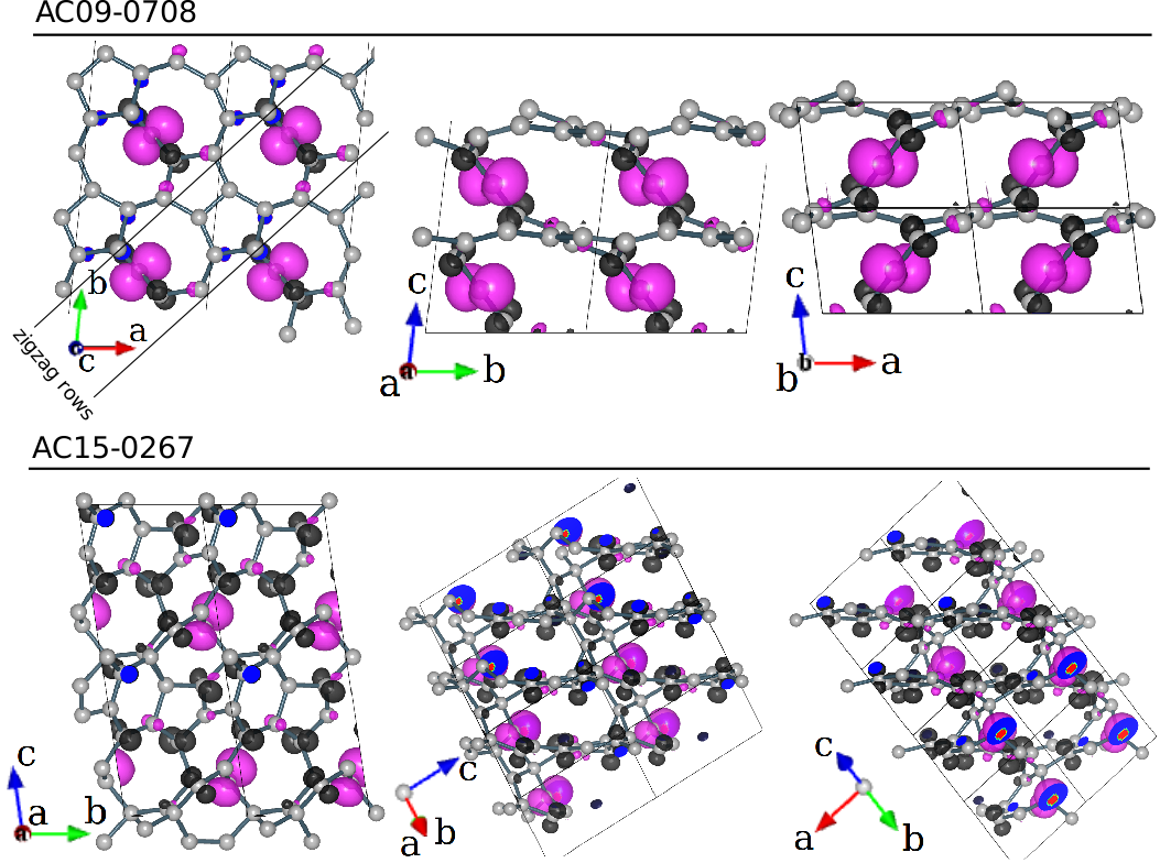
Figure 11: Spin density isosurface plot of the samples with 3D ferrimagnetic properties studied within GGA-PBE approximation.

The second example of graphite-like structure is AC14-0831 shown in Fig. 10. We can describe its structure as a graphite made of planes of graphene connected through an interplanar dimer C2 (atoms M1 and M2 in Fig. 10 left-middle). Moreover, each graphene plane has a grain boundary GB-Miller ; GB-Coraux ; Loginova2009 made of a continuous line of Stone-Wales 5-7-7-5 defects Stone-Wales . Another way to imagine the structure of this grain boundary is to join together two grains with zigzag edges reconstructed as zigzag-57 Koskinen2008 (Fig. 10 top-left). The interplanar dimer C2 forms one pentagon and one tetragon with bottom and top planes respectively (Fig. 10 left-middle). The tetragon is formed by bonds between the C2 dimer and two heptagons in the grain boundary in the graphene plane (atoms A and B in Fig. 10 left-top) while the pentagon is formed by bonds between the C2 dimer and 3 atoms belonging to the hexagons in the graphene plane (atoms C, D, E in Fig. 10 left-top). The parallel alignment of the A-B bond to the vector connecting the atoms C and D gives the possibility of connecting the planes through the interplanar dimer M1-M2 by forming a pentagon and a tetragon with planar arrangement.

The origin of the magnetic states in this configuration is again explained by the Lieb theorem Lieb-theorem ; Yazyev2010-report ; KatsnelsonBook since the $sp^{3}$ atoms C and D, belonging to the same sublattice, break the bipartite lattice symmetry. This situation is similar to the one encountered in the junction of a nanotube with a graphene ribbonribbon-tube . Also there, the 4-fold atoms brake the bipartite symmetry, leading to magnetic moments.

The last set of samples discovered in our search has a 3D ferro/ferri-magnetic structure with large values of $J$. The samples AC16-0070 and AC15-0776 studied by LDA-CA (point N4 and N9 in Fig. 7 top) have a complicated geometry that we do not show here because it cannot be described in a simplified way as done previously. Within the samples studied by GGA-PBE we select AC15-0267, AC10-1116 and AC09-0708 (4th, 5th and 12-th points in Fig. 7 bottom) and show two of them in Fig. 11. The sample AC15-0267 can be classified as a graphite-like geometry with modifications in the graphene plane (i.e. grain boundaries and/or point defects) and interplane atoms (see Fig. 11 left-middle) similar to the geometry of AC14-0831. One more example of magnetic states due to the presence of dangling bonds is given by the sample AC09-0708 shown in the right panels of Fig. 11. This sample also has a layered structure where the 2-fold coordinated atoms always connect two layers. Each layer itself is made of two pentagons and two octagons arranged along a line between two zigzag rows. A top view of the sample gives an image very similar to the high angle grain boundary found for graphene on Ni in ref. Lahiri .

All structures presented in this section are availableac-xsf-data in the xsf file format suitable for use in the VESTA program vesta .

VIII Conclusions

In this work we have presented the results of a massive, automated search of disordered carbon structures with magnetic states. We have tried to identify the common structural features present in the samples where magnetic moments appear. In our analysis we have used elements of graph theory and the analogy to structural motifs in graphene grain boundaries. We believe that our computational approach can lead to progress in the understanding of $s-p$ electron magnetism. This task is however still far from complete and the ways to create magnetic order are still elusive and will require further investigations.

References

- (1) Rode A, Hyde S, Gamaly E, Elliman R, McKenzie D and Bulcock S 1999 Applied Physics A 69(1) S755–S758
- (2) Rode A, Elliman R, Gamaly E, Veinger A, Christy A, Hyde S and Luther-Davies B 2002 Applied Surface Science 197-198 644–649
- (3) Rode A V, Gamaly E G, Christy A G, Fitz Gerald J G, Hyde S T, Elliman R G, Luther-Davies B, Veinger A I, Androulakis J and Giapintzakis J 2004 Phys. Rev. B 70(5) 054407
- (4) Wales D J, Miller M A and Walsh T R 1998 Nature 394(6695) 758–760
- (5) URL ftp://ftp.science.ru.nl/pub/tcm/ac/
- (6) Momma K and Izumi F 2008 J. Appl. Crystallogr. 41 653–658
- (7) Hohenberg P and Kohn W 1964 Phys. Rev. 136(3B) B864–B871
- (8) Kohn W and Sham L J 1965 Phys. Rev. 140(4A) A1133–A1138
- (9) Soler J M, Artacho E, Gale J D, Garcia A, Junquera J, Ordejon P and Sanchez-Portal D 2002 J. Phys.: Condens. Matter 14 2745–2779
- (10) Sanchez-Portal D, Ordejon P and Canadell E 2004 Principles and Applications of Density functional Theory in Inorganic Chemistry II 113 (Berlin: Springer)
- (11) Artacho E, Anglada E, Dieguez O, Gale J D, Garcia A, Junquera J, Martin R M, Ordejon P, Pruneda J M, Sanchez-Portal D and Soler J M 2008 J. Phys.: Condens. Matter 20 064208
- (12) Ceperley D M and Alder B J 1980 Phys. Rev. Lett. 45(7) 566–569
- (13) Perdew J P and Zunger A 1981 Phys. Rev. B 23(10) 5048–5079
- (14) Junquera J, Paz O, Sánchez-Portal D and Artacho E 2001 Phys. Rev. B 64(23) 235111
- (15) Perdew J P, Burke K and Ernzerhof M 1996 Phys. Rev. Lett. 77(18) 3865–3868
- (16) Rydberg H, Dion M, Jacobson N, Schröder E, Hyldgaard P, Simak S I, Langreth D C and Lundqvist B I 2003 Phys. Rev. Lett. 91(12) 126402
- (17) Boukhvalov D W and Katsnelson M I 2008 Phys. Rev. B 78(8) 085413
- (18) Troullier N and Martins J L 1991 Phys. Rev. B 43(3) 1993–2006
- (19) Kleinman L and Bylander D M 1982 Phys. Rev. Lett. 48(20) 1425–1428
- (20) Monkhorst H J and Pack J D 1976 Phys. Rev. B 13(12) 5188–5192
- (21) Generate and test search URL http://intelligence.worldofcomputing.net/ai-search/generate-and-test-search.html
- (22) Genetic algorithms URL http://intelligence.worldofcomputing.net/machine-learning/genetic-algorithms.html
- (23) Akhukov M A, Fasolino A, Gornostyrev Y N and Katsnelson M I 2012 Phys. Rev. B 85(11) 115407
- (24) Anglada E, M Soler J, Junquera J and Artacho E 2002 Phys. Rev. B 66(20) 205101
- (25) Harary F 1969 Graph theory (Addison Wesley publishing company)
- (26) Novoselov K S, Geim A K, Morozov S V, Jiang D, Zhang Y, Dubonos S V, Grigorieva I V and Firsov A A 2004 Science 306 666–669
- (27) Lieb E H 1989 Phys. Rev. Lett. 62(10) 1201–1204
- (28) Yazyev O V 2010 Rep. Prog. Phys. 73 056501
- (29) Katsnelson M I 2012 Graphene: Carbon in Two Dimensions (Cambridge University Press)
- (30) Zhou J, Wang Q, Sun Q, Chen X S, Kawazoe Y and Jena P 2009 Nano Letters 9 3867–3870
- (31) Koskinen P, Malola S and Häkkinen H 2008 Phys. Rev. Lett. 101(11) 115502
- (32) Miller D L, Kubista K D, Rutter G M, Ruan M, de Heer W A, First P N and Stroscio J A 2009 Science 324 924–927
- (33) Coraux J, N‘Diaye A T, Busse C and Michely T 2008 Nano Letters 8 565–570
- (34) Loginova E, Nie S, Thürmer K, Bartelt N C and McCarty K F 2009 Phys. Rev. B 80(8) 085430
- (35) Stone A and Wales D 1986 Chemical Physics Letters 128 501 – 503
- (36) Akhukov M A, Yuan S, Fasolino A and Katsnelson M I 2012 New J. of Phys. 14 123012
- (37) Lahiri J, Lin Y, Bozkurt P, Oleynik I I and Batzill M 2010 Nat. Nanotechnol. 5 326–329