Probing of the Interactions Between the Hot Plasmas and Galaxies in Clusters from to
Abstract
Based on optical and X-ray data for a sample of 34 relaxed rich clusters of galaxies with redshifts of , we studied relative spatial distributions of the two major baryon contents, the cluster galaxies and the hot plasmas. Using multi-band photometric data taken with the UH88 telescope, we determined the integrated (two dimensional) radial light profiles of member galaxies in each cluster using two independent approaches, i.e., the background subtraction and the color-magnitude filtering. The ICM mass profile of each cluster in our sample, also integrated in two dimensions, was derived from a spatially-resolved spectral analysis using XMM-Newton and Chandra data. Then, the radially-integrated light profile of each cluster was divided by its ICM mass profile, to obtain a profile of “galaxy light vs. ICM mass ratio”. When the sample is divided into three subsamples with redshift intervals of , , and , the ratio profiles over the central regions were found to steepen from the higher- to lower- redshift subsamples, meaning that the galaxies become more concentrated in the ICM sphere towards lower redshifts. A K-S test indicates that this evolution in the cluster structure is significant on % confidence level. The evolution is also seen in galaxy number vs. ICM mass ratio profiles. A range of systematic uncertainties in the galaxy light measurements, as well as many radius-/redshift- dependent biases to the galaxy vs. ICM profiles have been assessed, but none of them is significant against the observed evolution. Besides, the galaxy light vs. total mass ratio profiles also exhibit gradual concentration towards lower redshift. We interpret in the context that the galaxies, the ICM, and the dark matter components followed a similar spatial distribution in the early phase (), while the galaxies have fallen towards the center relative to the others at a later phase. Such galaxy infall is likely to be caused by the drag exerted by the ICM to the galaxies as they move through the ICM and interact with it, while gravitational drag can enhance the infall of the most massive galaxies.
1 INTRODUCTION
The X-ray emitting hot plasma in galaxy clusters, or the so called intracluster medium (ICM), with temperature of keV and number density of cm-3, constitutes about % of the detected baryon content in clusters. The remaining % resides in member galaxies, which move through the ICM with transonic speeds, km s-1, where , , , , and are the gravitational constant, cluster mass, radius of the galaxy orbit, mean molecular weight and the proton mass, respectively. Since two-body relaxation between dark matter halo and member galaxies occurs on timescales much longer than the time for a galaxy to cross the cluster (Sarazin 1988), the ICM-filled cluster volume is considered to be rather transparent to the moving galaxies from a pure gravitational point of view. From a fluid mechanics/plasma physics point of view, however, the member galaxies, which have their own plasmas (so called inter-stellar medium; ISM), are not totally collisionless with the ICM. Given the gas density and relative velocity, the galaxies have a cross section large enough for the ICM to be dragged significantly via, e.g., ram pressure (Gunn & Gott 1972; see also the review by Roediger 2009) and/or magnetohydrodynamical (MHD) effects (Asai et al. 2005, Makishima et al. 2001). Recent observations have revealed filamentary structures in HI associated with the moving galaxies (e.g., Oosterloo & van Gorkom 2005), in H (e.g., Yoshida et al. 2008), and also in X-ray images (e.g. Sun et al. 2006), which hint for such galaxy-ICM interactions. These urge us to study whether such interactions proceed efficiently in general or not, and how such interactions affect the spatial extents of the two baryon components.
When discussing the radial extents of the baryons, we must consider the following three important observational facts that are found among nearby clusters. (1) The stellar component is spatially much more concentrated than the ICM and the dark matter (e.g., Bahcall 1999). (2) On the central several tens to hundreds kpc scales, the ICM is considerably metal enriched, but the metals in the ICM are still much more extended than the stellar mass which must have produced them (e.g., Kawaharada et al. 2009; Sato et al. 2009). (3) In outer ( Mpc) regions of the Perseus cluster, the ICM metallicity remains relatively constant at (Simionescu et al. 2011). One possible explanation for (1) would be to assume that galaxies were formed in the past predominantly in core regions of the ICM and dark matter spheres. However, neither (2) nor (3) would be readily explained, unless assuming an extensive wind-driven outflow of metal-enriched gas at an expense of enormous energies ( erg; Kawaharada et al. 2009), or mechanical transport by active galactic nuclei (AGNs) of which the efficiency is still controversial (e.g., Vernaleo & Reynolds 2006). Alternatively, (1) alone could be explained if the ICM sphere grew by accretion of primordial gas after the initial galaxy formation was almost completed. However, this would also result in the same difficulty in explaining (2) and (3). Instead, the three observed facts can be consistently explained by the galaxy infall scenario proposed by Makishima et al. (2001). That is, the galaxies have been falling to the cluster center, presumably via galaxy-ICM interactions, while ejecting metals to the intra-cluster volume.
The present research on this subject has yet another interesting aspect, namely, ICM heating. The high ICM density ( cm-3) in cluster centers leads to significant energy losses by X-ray radiation, which can cool the gas down on a very short () timescale. However, broad-band X-ray imaging spectroscopy, starting with ASCA, found that the effect of cooling is much weaker than previously predicted (Makishima et al. 2001; Tamura et al. 2001; Peterson et al. 2001; Xu et al. 2002), suggesting that some significant heating mechanisms are in operation. Current solutions include energy injection from the central AGN (e.g., Churazov et al. 2001), heat inflow by thermal conduction (e.g., Zakamska & Narayan 2003), and turbulence and dynamical friction driven by galaxy motion (Kim & Narayan 2003; El-Zant et al. 2004). The numerical results of Ruszkowski & Oh (2011) indicate that the interaction between galaxies and ICM may give rise to subsonic turbulence in the ICM at a velocity of km s-1, and the turbulence can in turn boost heat transfer towards the cluster center so as to maintain the thermal stability of the ICM halo. Such a turbulent model gains observational support from the power spectrum analysis of gas pressure (Schuecker et al. 2004) and Faraday rotation (Vogt & Ensslin 2005) maps. At the same time, the galaxies, which empower the turbulent heating, should gradually lose their kinetic energy to the ICM and fall to the bottom of cluster potential (Makishima et al. 2001)
From the above pieces of evidence, it is suggested that the galaxies used to be distributed more widely to the edge of the ICM sphere (and the cluster potential), and have been falling to the cluster center, presumably over the Hubble time, as they are dragged by the ICM component. Furthermore, as shown in, e.g., Fujita & Nagashima (1999) and Quilis et al. (2000), such galaxy-ICM interactions would induce a burst of star formation in the onset of galaxy infall, and subsequently strip out most of the remaining cool disk gas. Hence, the idea of galaxy infall may also shed light on several observed phenomena of cluster galaxies, e.g., the truncated cool disk gas profiles and severe reduction of star formation in the center of the Virgo cluster (Koopmann et al. 2001; Koopmann & Kenney 2004), and the positive dependence of blue galaxy fraction on both the clustocentric distance (e.g., Whitmore et al. 1993) and redshift (e.g., Butcher & Oemler 1978).
By stacking the SDSS DR7 data of over 20000 optically-selected groups and clusters, Budzynski et al. (2012) recently reported that the galaxy density profile does not vary in shape over . However, by analyzing the spectroscopic and photometric data of 15 X-ray bright rich clusters at , Ellingson et al. (2001) showed an indication that the galaxy distribution gets more centrally-concentrated in lower redshifts (see their Fig. 9). Since the sample in the former study is dominated by groups and poor clusters (see their Fig. 1), where the hot gas density is much lower than that in the rich objects studied in the latter work, the difference in these two results possibly hints for galaxy infall dragged by the ICM. So far no systematic study has been made to compare directly the spatial extents of the galaxies and ICM for different redshifts, so that the role of galaxy-ICM interaction still remains rather unexplored. To address this issue, we jointly analyze in the present work high quality optical and X-ray data, and study the relative spatial distributions of the stellar component vs. the ICM component, for a sample of 34 X-ray bright massive galaxy clusters with a redshift range of to 0.9.
The layout of this paper is as follows. Section 2 gives a brief description of the sample selection and data reduction procedure. The data analysis and results are described in §3. We discuss the physical implication of our results in §4, and summarize our work in §5. Throughout the paper we assume a Hubble constant of km s-1 Mpc-1, a flat universe with the cosmological parameters of and , and quote errors by the 68% confidence level unless stated otherwise. The optical magnitudes used in this paper are all given in the Vega-magnitude system.
2 Observation and Data Preparation
2.1 Sample Selection
Our sample was primarily constructed based on previous X-ray flux-limited samples presented in Croston et al. (2008; 31 clusters), Leccardi & Molendi (2008; 48 clusters), and Ettori et al. (2004; 28 clusters), which contribute to the redshift ranges of , , and , respectively. All the three samples were originally constructed to study the ICM properties (e.g., density, temperature) of X-ray bright clusters using high quality Chandra and XMM-Newton data. This merged primary sample, comprising 107 () clusters, was further filtered through the following criteria. First, to study clusters with sufficient member galaxies and similar extent, the sample clusters should be massive and similar in scale. The 107 clusters were for this purpose filtered by their and , where is defined as a radius corresponding to a mean overdensity of the critical density at the cluster redshift, and is the total mass enclosed therein. To account for cosmic growth of the cluster halo, we further calculated the expected mass and scale for each cluster after experiencing evolution down to , i.e., and , respectively, with a redshift-dependent factor derived from a CDM numerical simulation of Wechsler et al. (2002; see actual form of the factor in §3.5.2). Systems with and with in the range of kpc were selected. This reduced the number of candidates to 98. Second, to avoid strong merging clusters, the positions of the X-ray brightness peak and the central dominant galaxy are required to coincide with each other within 50 kpc, and the X-ray morphology should be approximately symmetric. By examining the archival optical (DSS) and X-ray (XMM-Newton and Chandra) images of the 98 candidates, we finally selected 34 clusters that also survive the second criterion. Basic information for the 34 clusters are shown in Table 1. The sample was further categorized into three subsamples by their redshifts, i.e., low-redshift subsample (, hereafter subsample L), intermediate-redshift subsample (, hereafter subsample M), and high-redshift subsample (, hereafter subsample H).
The most important strategy of our study is to compare the X-ray and optical profiles of each cluster in the sample, to suppress the effects of intrinsic scatter in the cluster richness. As described in §2.2, the X-ray data for this purpose are readily available in archives. A more difficult part is the optical information, because we need to determine the galaxy membership in each cluster. For this purpose, however, existing archival optical databases (e.g., DSS, SDSS, 2MASS) either cannot fully cover our sample, or are not deep enough for accurate galaxy light measurements, especially for high redshift clusters. Hence, we utilized the University of Hawaii 88-inch (UH88) telescope to observe the 34 clusters with deep optical photometric data (PI: Inada). The UH88 telescope is suited to our study, since its field of view, , can cover, even in the nearest objects in our sample, the central Mpc regions where the galaxy-ICM interactions are mostly expected to take place. Details of the observations are given in §2.3.
2.2 X-ray Data
To achieve relatively homogeneous spatial resolutions for low redshift and high redshift clusters, we use XMM-Newton data for and Chandra data for clusters, since Chandra has a narrower point-spread-function than XMM-Newton by an order of magnitude. As shown in Table 2, all the necessary X-ray data are available in the archive.
2.2.1 Chandra
We used the newest CIAO v4.4 and CALDB v4.4.7 for screening the Chandra data obtained with its advanced CCD imaging spectrometer (ACIS). First, the bad pixels and columns were removed, as well as events with ASCA grades 1, 5, and 7. We then executed the gain, CTI, and astrometry corrections. By examining keV lightcurves extracted from source free regions near the CCD edges (e.g., Gu et al. 2009), we removed the time intervals contaminated by occasional background flares with count rate % of the mean value. When available, ACIS-S1 data were also used to crosscheck the determination of the contaminated intervals. As shown in Table 2, the exposure time was reduced by ks for MS2053 and RXJ1334, and by ks for the other clusters. In the ACIS spectral analysis, bright point sources were detected and removed with the CIAO tool celldetect. The spectral ancillary response files and redistribution matrix files were calculated with the CIAO tools mkwarf and mkacisrmf, respectively.
Following Gu et al. (2012), the background was determined based on fitting a spectrum extracted from an off-center region, which is Mpc away from the cluster center, with co-addition of cosmic X-ray background (hereafter CXB), non-X-ray background, Galactic foreground, and cluster emission components. Following, e.g., Markevitch et al. (2003), the non-X-ray background spectra were obtained from stowed ACIS observations. After subtracting this component, we fitted the resulting spectrum with an absorbed power law model (photon index ) describing the CXB, an absorbed APEC model (temperature = 0.2 keV and abundance = 1 ) for the Galactic foreground, and another absorbed APEC model for the cluster emission. The average keV CXB flux was estimated to be ergs cm-2 s-1 sr-1, which is consistent with the result of Kushino et al. (2002). The typical uncertainties on the CXB flux are % and % for high-count and low-count datasets, respectively, which were accounted for in determining the error range of ICM mass profiles (see §3.2 for details).
2.2.2 XMM-Newton
Basic reduction and calibration of the XMM-Newton European Photon Imaging Camera (EPIC) data were carried out with SAS v11.0.1. In the screening process we set FLAG = 0, and kept events with PATTERNs 0–12 for the MOS cameras and those with PATTERNs 0–4 for the pn camera. By examining lightcurves extracted in keV and keV from source free regions, we rejected time intervals affected by hard- and soft-band flares, respectively, in which the count rate exceeds a 2 limit above the quiescent mean value (e.g., Katayama et al. 2004; Nevalainen et al. 2005). The obtained MOS and pn exposures are shown in Table 2. Point sources detected by a SAS tool edetect_chain were discarded in the spectral analysis. The tool xissimarfgen and xisrmfgen were used to calculate the ancillary responses and redistribution matrixes, respectively. Like in the ACIS analysis, the EPIC background was determined by fitting a CCD-edge region, which locates Mpc away from the cluster center, with combined CXB, non-X-ray background, Galactic foreground, and the cluster emission components. The wheel-closed datasets were used as the non-X-ray background. The average keV CXB flux was measured to be ergs cm-2 s-1 sr-1, again in agreement with Kushino et al. (2002). The typical error of the CXB flux, %, was used for calculating the uncertainty on ICM mass profiles (see §3.2 for details). Spectra of the three EPIC detectors, MOS1, MOS2, and pn, were fitted simultaneously with the same model, but leaving the model normalization free for each dataset.
2.3 Optical Data
As summarized in Table 3, optical images of our sample clusters were obtained with the UH88 telescope on six nights in February, March, and August of 2010. The February and August observations were carried out with the thinned Tek 2K CCD mounted at the f/10 RC focus in , , and , and in March the targets were observed with the Wide Field Grism Spectrograph 2 (WFGS2) in , , and imaging mode. Besides the central pointing of each cluster as described above, we observed an offset region in or , which is about ( Mpc) away from the central galaxy. The central and offset pointings were made with similar observation depth. All images have a pixel scale of . The exposure and limiting magnitude for each pointing are given in Table 3.
The data were reduced with the IRAF software following the standard procedure as described in Kodama et al. (2005). First, the images in each band were debiased and flattened using a median of dome-flat images in the same band taken before the cluster observation. For each cluster the dithered images in the same band were shifted into registration and combined after rejecting cosmic rays. As summarized in Table 3, the resulting images have a typical seeing of . Astrometry calibration was performed using the USNO-A2.0 catalog (Monet 1998), and the photometric zero points were calibrated based on the standard star data of Landolt (1992) and Fukugita et al. (1995) in and bands, respectively. According to the transformation equations in Lupton (2005), the , , and magnitudes were converted into those in the , , and bands, respectively.
Object identifications and flux measurements were performed with the Source Extractor algorithm (SExtractor; Bertin & Arnouts 1996), and sources with at least 10 connected pixels (comparable to the spatial resolution of the observations ), of which the signal is higher than 3 above the contiguous background intensity, were considered as a detection of an object. To separate stars and galaxies, we constructed a star catalog based on the neural network method in SExtractor. All the objects with CLASS_STAR 0.6 measured by SExtractor were classified as stars and were excluded from the subsequent analysis. The -band images were used in the star detection, and - and - band images were used for crosscheck. The Kron-type total magnitudes and fluxes (MAG_AUTO and FLUX_AUTO, respectively) were measured using automatic aperture with the minimal value of ( kpc for different redshifts). We inspected the aperture maps and confirmed the absence of strong aperture overlap between neighboring objects. The galaxy color was measured in the double image mode, which ensures the same elliptical aperture between the different bands.
The calibrated apparent magnitude was transformed to absolute magnitude by applying the relation,
| (1) |
where is the luminosity distance, is the Galactic extinction computed using the Galactic map of Schlegel et al. (1998), and is the K-correction. We used the band-dependent K-correction by Fukugita et al. (1995) for early-type galaxies, which are assumed to be the dominant population of the sample clusters.
2.4 Determinations of and the Cluster Center
To compensate for the differences in the cluster scale, we normalize all the galaxy light and ICM mass profiles obtained in the subsequent analysis to the scale of each cluster, which can be characterized by . To avoid possible systematic errors in the determinations among different authors (Table 1), we did not use the given in literature. Instead, was estimated based on an empirical relation using the average ICM temperature as (Finoguenov et al. 2001), where is the cosmological evolution factor. was calculated based on spectral fitting of the cluster central 500 kpc region X-ray data, but excluding the innermost 100 kpc to avoid the temperature affected by a cool ICM component that is often found therein. Specifically, the background-corrected EPIC/ACIS spectra were fit with an absorbed, single-temperature APEC model in keV, with the ICM temperature and abundance set free. The obtained and , listed in Table 4, agree with the previous results quoted in Table 1 within 25% and 20%, respectively. We have tested another relation presented in Zhang et al. (2008), which was obtained with a combined weak lensing and X-ray study. The estimated from the two relations are consistent within %.
Next, we determined the cluster center by comparing three types of centers, i.e., optical peak of the brightest galaxy (Center I), X-ray brightness peak (Center II), and centroid of the cluster X-ray surface brightness over a central region (Center III). To calculate Center III, we applied a CIAO task dmstat on a region centered on the X-ray peak. After the centroid was derived, we started an iteration based on the new centroid. To approach the cluster center region, the new examining radius was set to be . The iterations were regarded as converged when the centroid shifts by less than . As shown in Table 4, the offsets among Center I, II, and III were smaller than 50 kpc (). Since Center III is less affected by core disturbances (e.g., AGN activity and cD galaxy sloshing) than the other two centers, we employed it for the subsequent analysis. Our results remain virtually the same even using Center I or Center II.
3 Data Analysis and Results
3.1 Optical Light Profiles
To calculate the radial profiles of the stellar light, we first need to define the galaxy membership of each cluster. However, it is difficult to perform this directly, since there is no spectroscopic data available for the cluster sample observed with UH88. Generally this problem may be overcome in two approaches. One is to subtract the foreground and background galaxy contributions, based on the surface brightness of field galaxies in the offset pointing data. The other is to set color filter in the color-magnitude space, as the red sequence member galaxies, which contribute a majority of cluster membership in the central region, are expected to show a well defined relation on the color-magnitude diagram. The former background subtraction (hereafter BS) method is mainly subject to uncertainties due to cosmic variance, arising from random projections of large scale structures, while the latter color-magnitude filtering (hereafter CMF) method may suffer biases by underestimating blue member galaxies. To minimize the expected biases, we employ both the BS and CMF approaches in our analysis.
3.1.1 Background Subtraction
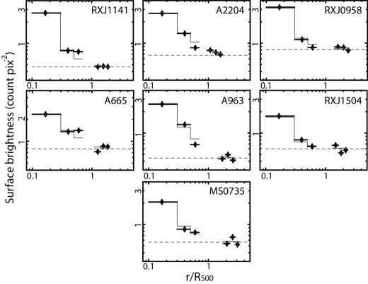
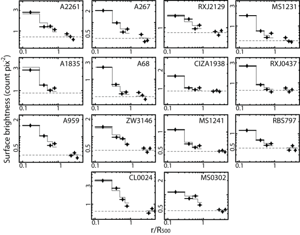
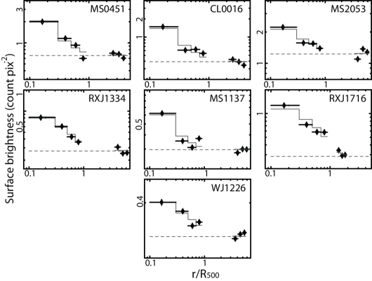
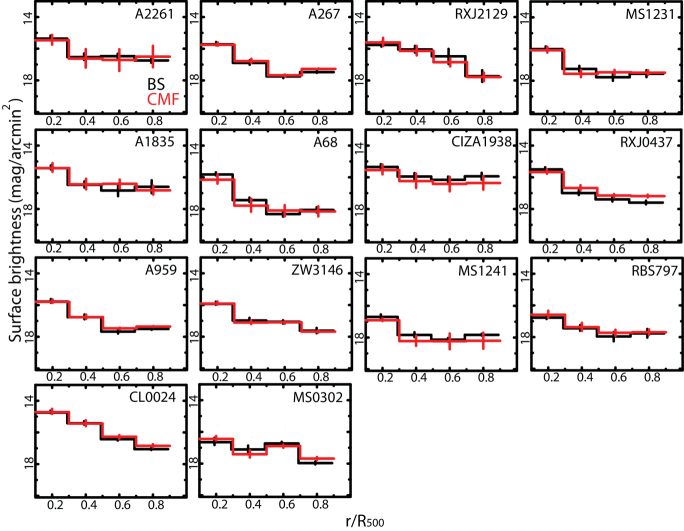
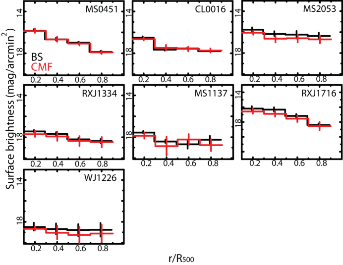
The BS method has been widely used to measure the cluster galaxy luminosity (e.g., Abell 1958; Valotto et al. 1997; Goto et al. 2002; Hansen et al. 2005). First, we divided the -band images of the central pointings into four radial bins, i.e., , , , and . This binning was chosen because each bin contains a sufficient number of detected galaxies (at least 30, typically ) before background subtraction. For the subsample-L clusters, the outermost radial bin was omitted in the actual measurement, because it was only partially covered by the central pointing. To exclude apparent foreground galaxies, those with fluxes (FLUX_AUTO) higher than the cluster central galaxy were discarded from the surface brightness calculation. Then we estimated the background contribution based on data of the offset regions about Mpc ( ) away from the cluster center, which were observed with similar depth and seeing as the cluster central regions (; Table 3). Bright foreground galaxies with fluxes higher than the central galaxies were again removed. To discard any possible background clusters or voids in the offset region, we divided it into 3 sub-regions, each with a size of , and discarded those sub-regions which have a galaxy number deviated from the mean value by . To measure the surface brightness profile of the remaining offset region, we re-divided it into three radial annuli centered on the central galaxy, each with a width of , and calculated the galaxy flux per unit area for each bin. The obtained central + offset surface brightness profiles for six representative clusters (two for each subsample) are shown in Figure 1 (see also Fig. A.1 for the other clusters).
Figure 2 shows surface brightness profiles from the offset regions, averaged over the three subsamples (L, M, and H). These profiles were calculated by summing up, over the relevant subsample, those galaxies which fall in a radial bin with a width of , and then dividing by the sky area. Thus, the results still show a mild outward decline, suggesting that the cluster galaxies should distribute up to . Considering this, we fit the combined central + offset -band surface brightness profiles with a King model plus constant, (King 1962), where is a normalization, is projected radius, is core radius, and represents the background component. As plotted in Figure 1, this model gave reasonable fits to the combined (central plus offset) surface brightness profiles of the six representative clusters, as well as to the rest, all with (Table 5). As shown in, e.g., Budzynski et al. (2012), the cluster galaxy distributions can also be described by a Navarro-Frenk-White model (Navarro, Frenk, & White 1996, hereafter NFW model), which was first introduced to describe dark matter distributions. We fit the surface brightness profiles by , with , where is the projected scale radius. The results of this fit are also given in Table 5. Thus, the two models yield essentially similar cluster galaxy components for the offset region, so that the background components obtained with the two fittings are consistent with each other within errors (Table 5). Therefore, we selected from the fit whichever gave a smaller . Then, by subtracting this from each radial bin in the central region, we obtained the member galaxy surface brightness profiles as shown in Figure 3 (see also Fig. A.2).
The error of the obtained surface brightness profiles is dominated by statistical uncertainties of the data, as well as systematic uncertainties of the background which originates from the cosmic variance, i.e., the galaxy luminosity variations due to the spatial distributions of large-scale structures. To quantify this effect, we adopted a theoretical result of Trenti and Stiavelli (2008), who provide analytic estimation of galaxy number fluctuation as a function of region size and the target redshift. Their calculation is based on a two point correlation function of galaxy halos generated with Press-Schechter formalism. In this way, the fractional background uncertainties in our analysis were estimated to be and for low-redshift and high-redshift ends, respectively. The final error bars shown in Figure 3 and Figure A.2 were obtained by combining in quadrature the systematic background uncertainty and the statistical flux measurement error.
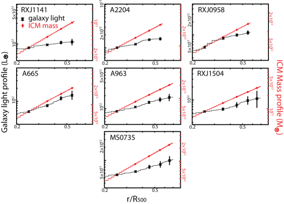
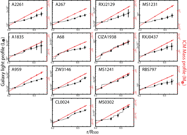
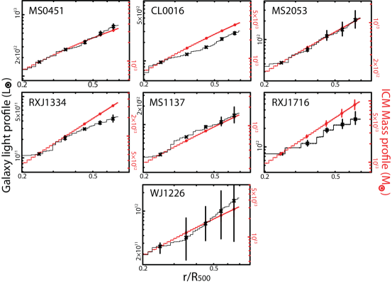
The background-subtracted surface brightness enclosed in radius was integrated to calculate the integral light profile, . Figure 4 and Figure A.3 show the result for each cluster, in the form of a quasi-continuous integrated light profile. This was obtained by adding up all galaxies (including background) detected in I-band, and then subtracting the background contribution which scales as the radius squared. At the same time, based on the surface brightness uncertainties obtained above, we evaluated error ranges at five representative radii, i.e., , , , , and . The typical errors are % and % for and , respectively.
3.1.2 Color-Magnitude Filtering
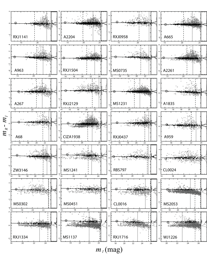
To cross-check the background subtraction result, we conducted the member galaxy selection based on the standard color-magnitude relation, that the old passively evolving cluster galaxies form a tight horizontal relation in the color-magnitude space (Bower et al. 1992; Stanford et al. 1998; Kodama et al. 1998). The colors were acquired from the Kron-type - and - band magnitudes calculated with the SExtractor, and corrected for photometric zero points as described in §2.3. As shown in Figure 5 (also seen in Fig. A.4), the bright red sequence galaxies form an apparent ridge-line with weak negative slopes. This line-up creates a peak on the projected number-color histogram shown in the right side panels of Figure 5. First, a Gaussian fitting to the number-color histogram was used to determine the approximate color range which contains the color-magnitude line. The fitting gave an approximate central color (), as well as the associated color dispersion (). For the high redshift ones (), we set to the color of the central dominant galaxy and , as the relatively high background level caused poor determinations of the central color. Then, to further determine the slope of the relation, we performed linear fitting, = + , where and are free parameters, to the color-magnitude diagram over a color range and a magnitude range . The fitting was optimized with a robust biweight linear least square method (Beers, Flynn & Gebhardt 1990), which is insensitive to data points much deviated from the relation, e.g., foreground/background galaxies. The fitting was repeated for a few times, as the data points outside the 3 range of the fitted relation were rejected in the next iteration. Typically, the color-magnitude relation fitting converged within less than five iterations. The derived relations, characterized by the best-fit parameters and listed in Table 5, are consistent with the predicted redshift-dependent relations reported in Kodama et al. (1998). Then the red-sequence members were selected as data within the fitting uncertainty range of the derived relations, typically mag (Figure 5, Table 5). The integral light profiles, , were obtained based on the fluxes of the selected galaxies.
According to e.g., Kodama & Bower (2001), the faint end of the color-magnitude relation is strongly contaminated by background non-members that by chance fall in the same range as the members. To remove such faint-end contaminants, candidates with apparent were discarded. To account for the background contaminants on the brighter part of the red sequence relation, we followed Hao et al. (2009) and fit the color diagram of non-selected galaxies with a Gaussian model. By integrating the best-fit model over the color range of red sequence relation, we estimated the number of non-member contaminants to selected galaxies. In this way, the systematic uncertainty of the CMF method was estimated to be %, which is comparable to those shown in Kodama & Bower (2001). Assuming a uniform spatial distribution of the non-members, the error was propagated to each radial bin to define the systematic uncertainty of the integral galaxy light profile.
Another source of uncertainty is the fitting error of the color-magnitude relation, which was assessed with Monte-Carlo simulations. Following, e.g., Hilton et al. (2009), the color of each galaxy has been replaced with a random variable within its measurement error, and the randomized color-magnitude diagram was fitted with the robust regression method. By 1000 realizations for each cluster, we determined the errors on the slope and intercept of the relation, and hence the uncertainty of the galaxy flux caused by fitting. In Figure 3 and Figure A.2, the systematic and fitting errors are combined in quadrature and used as the final error range of the profiles.
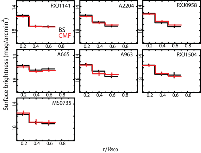
The member selection results obtained with the BS and the CMF methods were cross-examined for consistency in two ways, the radial surface brightness profile and the luminosity function. In Figure 3 (see also Fig. A.2), we compare the surface brightness profiles obtained with the two methods. In most bins the two profiles agree with each other within error ranges. Their differences, mainly caused either by local background variations in the BS method or the omission of blue populations in the CMF, are thus found to be on average % to 20% from innermost to outermost bins, respectively. In addition, the luminosity function of the entire member galaxies, detected in our 34 sample clusters, was constructed using the BS and CMF methods separately. For the BS method, this was performed by subtracting another luminosity function created from the offset regions of the 34 clusters. We excluded the central dominant galaxies, which are known to be outliers in this respect. As shown in Figure 6, the two methods again give consistent luminosity functions.
To compare our luminosity functions with previous works, two best-fit functions in Rudnick et al. (2009) are also plotted in Figure 6. Their curves were given in the Schechter form (Schechter 1976) as
| (2) |
where is the galaxy number, is normalization, while and are parameters defining the shape of the function. The two curves from Rudnick et al. (2009) are defined by shape parameters () = (-21.46, -0.75) and (-21.83, -0.58), which were obtained for local clusters with and high redshift ones with , respectively. Our sample-averaged BS and CMF results are consistent with both curves within errors. The agreement between our results and their local cluster curve can be represented by = 2.8/5 and 2.5/4 for the BS and CMF curves, respectively, which is slightly better than that with the high redshift one, = 4.1/5 and 5.5/4 for the BS and CMF curves, respectively. This is probably because most (two-thirds) of our sample clusters have redshifts below 0.4. Hence, we have proved the agreement between the BS and CMF radial light profiles, which are also well in line with those reported in previous optical studies.
3.2 X-ray Mass Profiles
To derive cluster gas mass profiles, the gas density profiles were calculated based on deprojection spectral analysis with the XMM-Newton EPIC and Chandra ACIS data after point source removal and background correction (§2.2). First we extracted spectra from several concentric annulus regions for each cluster. The radial boundaries of each annulus, and , were chosen by and 1.25 for high-flux clusters and low-flux ones, respectively. The extracted spectra were fit in keV with an absorbed, single-temperature APEC model in XSPEC. All annuli were linked by a PROJCT model, which evaluates a two-dimensional (hereafter 2-D) projected model from intrinsic three-dimensional (hereafter 3-D) one; in this way all the APEC parameters are obtained in 3-D. For each 3-D annulus, the gas temperature and metal abundance were set free. When the model parameters cannot be well constrained in some annuli due to relatively low statistics, we tied them to the values of their adjacent regions. The column density of neutral absorber was fixed to the Galactic value given in Kalberla et al. (2005). All the fits were acceptable, with reduced chi-square for a typical degree of freedom of . Then, the 3-D gas density profiles were calculated from the best-fit model normalization of each annulus; the ICM density is proportional to the square root of the model normalization. The results are presented in Figure 7 (see also Fig. A.5), where the density error bars were obtained by taking into account both statistical and systematic uncertainties. The former was estimated by scanning over the parameter space with an XSPEC tool steppar iteratively, while the latter was assessed by re-normalizing the level of CXB component by 20% (§2.2) for each annulus.
As shown in Figure 7 and Figure A.5, the gas density profiles were fit with a canonical model, , where is the core radius and is the slope. In several clusters (i.e., A963, A1835, A68, A1576, RBS 797, MS0451, and CL0016), the observed profiles show significant central excess over the model. Such an excess often indicates a hierarchical potential structure associated with the cD galaxy, sometimes augmented by the central cool component (see Makishima et al. 2001 for a review). In these clusters the ICM density profiles are empirically better described with a double- model, , where suffixes 1 and 2 indicate the compact and extended components, respectively. Actually in previous works, this model successfully described the ICM emissivity profiles of some representative cool-core clusters (e.g., Ikebe et al. 1999; Xu et al. 1998). To reduce degeneracy among the double- parameters, we fixed in the fittings. Allowing them free does not change the resulting model profile significantly. For the seven clusters showing the central excess, the double- model yields significantly better fit than the model with reduced chi-square . The best-fit parameters for the /double- models are listed in Table 4. Like in the optical case, we calculated the 2-D ICM mass profile, , by projecting the best-fit /double- density profile along the line of sight, and integrating it over the 2-D radius. The obtained quasi-continuous 2-D ICM mass profiles are shown in Figure 4 and Figure A.3, together with the errors estimated at , , , , and . The typical uncertainties at are % and % for high flux and low flux clusters, respectively.
3.3 Galaxy Light vs ICM Mass Ratio Profiles
As revealed in Figure 4 and Figure A.3, the profiles of L-subsample clusters are significantly flatter than their profiles. In contrast, the optical and X-ray profiles of H-subsample clusters show similar gradients. To enable direct comparison between their slopes, we normalized each of them to its central values within , and calculated the ratios between the normalized profiles. This gives “galaxy light vs. ICM mass ratio” (hereafter GLIMR) at each radius, together with the uncertainties at the representative points selected in Figure 4; , , , and . In Figure 8, we present the subsample-averaged GLIMR profiles obtained with the BS and CMF methods. Uncertainties of the averaged profiles were calculated by combining in quadrature the errors of all clusters in the subsample. The BS-GLIMR profiles are consistent with the CMF-GLIMR ones within 1 error range.
As shown in Figure 8, the average GLIMR profiles of the subsample L clusters drop steeply towards outer regions, reconfirming the inference of Figure 4 and Figure A.3. The GLIMR profiles of the subsample H clusters, in contrast, show significantly flatter distributions than the low redshift counterparts, and the profiles of the subsample M clusters appear to have intermediate gradients. The normalized BS-GLIMR at are , , and for the subsample L, M, and H, respectively. The CMF method gave consistent values, , , and for the subsample L, M, and H, respectively. The galaxy and ICM components thus followed a similar distribution in high-redshift () clusters, while their optical size relative to that of ICM evolved to become considerably smaller within central in nearby () systems.
To confirm that Figure 8 reflects systematic differences among the three subsamples, rather than, e.g., biased by some extreme outliers, we carried out Kolmogorov-Smirnov (K-S) test among the three subsamples. In Figure 9 we show the cumulative fraction probability distributions as a function of the GLIMR values of individual objects at and . The K-S probability curves are clearly separated among the three subsamples. Given the D-statistics shown in Figure 9, the hypothesis that the BS-GLIMRs follow the same distribution at can be rejected at and confidence levels between subsamples L and M, and between subsamples M and H, respectively. The CMF-GLIMR profiles show similar significance, that the hypothesis can be rejected at and levels between subsamples L and M, and between M and H, respectively. To account for the measurement uncertainties, we performed 1000 Monte-Carlo realizations, in which the GLIMR profiles of the individual clusters were randomly varied within the error range. The D-statistics were not found to vary significantly.
To examine whether the gradient of GLIMR profile evolves with redshift continuously or not, we plot in Figure 10 the logarithmic slopes of the GLIMR profiles of the 34 clusters, defined as indices of the power-law models which best fit the five radial GLIMR points of each cluster, against cluster redshifts. The figure shows a smooth trend, that the logarithmic slope changes gradually from for the nearest objects to for the farthest ones. By fitting the distribution with a constant model, we obtained (BS) and (CMF) for . This means that the evolution of the GLIMR slope is significant at confidence level. Thus, the implication of Figure 10 agrees with those of Figure 8 and Figure 9.
3.4 GLIMR Profiles with the SDSS Data and Spectroscopic Measurements
To crosscheck the GLIMR profiles obtained with the UH88 data, we carried out an independent photometric analysis of SDSS DR6 (data release 6) public data (Adelman-McCarthy et al. 2008). As shown in Figure 11, a total of nine clusters in our sample were found available in the current SDSS DR6 catalog. From the catalog we obtained -band magnitudes for all galaxy-type objects (CLASS = 3) within , and their magnitudes were converted to fluxes to calculate surface brightness profiles. Galaxies with fluxes higher than that of the central dominant galaxy were excluded. For the remaining galaxies we applied the BS method (§3.1.1), wherein the background value was obtained by the average galaxy flux in an annulus with Mpc centered on the cluster center. To remove possible contamination from other clusters, the background region was divided equally into 20 azimuthal sectors, and those sectors of which the flux is deviated from the annulus-average value by 2 were discarded. After subtracting the background value from the surface brightness profile, the integral light profile, and hence the GLIMR profile was obtained in the same way as described in §3.3. The SDSS profiles have smaller uncertainties than the UH88 profiles, because the SDSS data have much better sky coverage for both source and background regions. As shown in Figure 11, the typical differences between the SDSS BS-GLIMR profiles and UH88 BS-GLIMR profiles are within 8% at all radii, which are smaller than the estimated error bars.
Multi-object spectroscopy gives the most reliable determination of galaxy members. Previous spectroscopic studies have provided membership information for five clusters in our sample, i.e., A959 (Boschin et al. 2009), RXJ2308 (Braglia et al. 2009), CL0024 (Moran et al. 2007), MS0451 (Moran et al. 2007), and CL0016 (Dressler & Gunn 1992), each with detected members in . By calculating the -band fluxes with the UH88 data for the spectroscopically confirmed member galaxies, we obtained the GLIMR profiles as shown in Figure 11 in blue. The spectroscopic GLIMR profiles are consistent with our photometric (either BS or CMF) GLIMR profiles within errors. The average fractional differences between the spectroscopic- and the BS- (CMF-) GLIMR are about 6% (10%), which agree with the systematic errors estimated in §3.1.1 and §3.1.2 for the BS and CMF methods, respectively.
For a further comparison, we examined the GLIMR profile of a typical relaxed cluster in local universe, Abell 1650 (hereafter A1650; ; keV; Donahue et al. 2005). While this cluster satisfies the criteria used in our sample definition, it is located closer than those in subsample L. Furthermore, its spectroscopic membership is available in Pimbblet et al. (2006). By deriving the converted -band profile of the spectroscopic members using the SDSS photometric data, and combining it with the ICM density profile measured in Gu et al. (2009; see their Fig. 2), we calculated the GLIMR profile of A1650 and compared it with our cluster sample. As shown in Figure 8, A1650 has an even more centrally-concentrated GLIMR distribution than the average profile of subsample L. This reinforces the GLIMR evolution detected in §3.3.
3.5 Systematics Errors and Biases
So far, we have detected significant evolution in the galaxy light-to-ICM mass ratio profiles among subsamples L, M and H. However, the result might be subject to various systematic errors and biases. In Figure 12, new five-point GLIMR profiles are presented to account for these effects one by one.
3.5.1 Possible Biases in High Redshift Clusters
First of all, the GLIMR evolution could be an artifact caused by the inconstant galaxy selection completeness, which obviously becomes lower at higher redshifts. To assess this redshift-dependent bias, we set a uniform absolute magnitude limit to the CMF method which corresponds to the observation depth at for the highest redshift cluster WJ1226. This limit was converted for each cluster to -band magnitude, and is shown as dashed lines in Figure 5 and Figure A.4. When galaxies fainter than this limit are discarded, the selection completeness applied to each cluster should be approximately the same. As shown in Figure 12a, the average CMF-GLIMR profile with the new limiting magnitude is consistent, within errors, with the previous one for each subsample; the difference caused by varying the limiting magnitude is about 5%. The BS method yielded similar results by applying the new limiting magnitude. Hence, the result is robust against the galaxy selection completeness.
As shown in, e.g., Cucciati et al. (2012), galaxies at high redshift tend to have more dust than those in local universe. The mean dust attenuation in far ultraviolet band increases by about 1 mag from to . This introduces a systematic uncertainty to the GLIMR profiles, especially for subsample H. This effect can be addressed by considering several observational facts. As shown in e.g., Garn & Best (2010), the dust attenuation has a positive correlation with the star forming rate, while such activity is known to become more enhanced towards outskirt regions of clusters with (e.g., Kodama et al. 2004; Koyama et al. 2008). Hence, the dust would more strongly attenuate the light emitted from cluster outer regions, and the effect should be stronger in higher redshift. However, this is opposite to the observed GLIMR evolution. Therefore, it is unlikely that the dust effect, if any, has significantly affected our results.
Since the cluster-average X-ray source-to-background ratio is generally smaller in more distant objects, it is possible that the ICM density profiles at are suppressed due to background over-subtraction in high redshift clusters, and the GLIMR profiles are biased to be flatter. To examine this effect, we calculated the X-ray source-to-background ratio at ( hereafter) for each cluster as shown in Table 4. The mean ratios are 1.7, 1.2, and 1.5 for subsample L, M, and H, respectively. These are larger than the limiting source-to-background ratio in previous studies using Chandra and XMM-Newton data (e.g., ; Leccardi & Molendi 2008), and are not strongly subsample dependent. Then we divided the 34 clusters into two groups by the mean source-to-background ratio (). As shown in Figure 12b, the average GLIMR profiles of the two groups are consistent with each other within errors. This indicates that the shape of the GLIMR profile is nearly independent of the X-ray source-to-background ratio, and the observed evolution cannot be explained by background over-subtraction of the X-ray data of high redshift clusters.
3.5.2 Possible Scale- and Richness- Dependences
To examine the uncertainty of the determinations based on the scaling relation (§2.4), we calculated a new set of directly from the hydrostatic mass estimates using the X-ray data. Based on the best-fit 3-D gas temperature profiles and density profiles obtained with the deprojected analysis (§3.2), and assuming spherical symmetry and a hydrostatic equilibrium, the total gravitating mass within a 3-D radius can be calculated generally as
| (3) |
where is the gravitational constant, is the average molecular weight, and is the proton mass. Then we calculated according to its original definition, i.e., the radius within which the average mass density equals to 500 times the critical density of the Universe. In Table 6 the new (re-named as for clarify) are shown, together with the total enclosed gravitating mass . The obtained and are consistent within 1 uncertainties with the previous measurements using both X-ray (e.g., Arnaud et al. 2007 and Zhang et al. 2008) and weak lensing (e.g., Dahle 2006) techniques. By adopting , the BS-GLIMR profiles were updated as shown in Figure 12c. The new profiles are consistent with the previous ones within 1 errors, and the different measurements of introduce insignificant (%) bias on the GLIMR profile.
Since our sample clusters have a non-negligible scatter in the system richness, it is important to examine whether or not the gradient of GLIMR is related to the cluster mass. Since some ICM heating processes, e.g., AGN outbursts (see McNamara & Nulsen 2007 for a review), are expected to have stronger effects of expelling hot gas in systems with shallower potentials (Sun et al. 2009), the gas mass profiles might be more extended in such systems. Since the stellar component would not feel such heating processes, the GLIMR profiles could be steeper in low-mass systems than in high-mass ones. In addition, there can be other unknown richness-dependent effects that may affect the GLIMR profiles. Because the higher-redshift subsamples would tend to pick up relatively richer clusters, the possible GLIMR dependence on cluster mass might mimic the observed evolution shown in Figure 8. We therefore divided each subsample equally into two subgroups according to the obtained as listed in Table 6, and compared the subgroup-average BS-GLIMR profiles. As shown in Figure 12d, the higher-mass subgroups do have slightly more extended GLIMR profiles as expected. However, the differences between them are within 6%, smaller than the errors. Both high-mass and low-mass profiles show essentially the same evolution. Hence, the systematic errors due to cluster mass differences do not significantly affect our result, and we can exclude the possibility that the GLIMR evolution is an artifact produced by the selection effect on cluster mass.
Since the clusters are expected to grow via long-term matter accretion from cluster outskirts, the cluster scale (i.e., mass and radius) should increase over several Gyrs. Therefore, a young cluster may have been growing by taking in infalling new materials, and eventually constitute a central region of an old cluster. In another word, the region of a subsample L cluster might correspond to a region in a subsample H cluster. To compensate for the underlying difference in cluster evolution stage, we again considered the evolved scale, , which was defined in §2.1 as the radius that each will evolve to at . Based on the empirical cosmic growth function derived from CDM numerical simulations, e.g., Wechsler et al. (2002), the cluster mass is expected to increase by a factor of from to , so that the can be estimated as , where is the cosmological evolution factor defined in §2.4. By adopting the new radial scale, the BS-GLIMR profiles were calculated in the same way as in §3.1.1. As shown in Figure 12e, the new BS-GLIMR profiles are consistent with our original results within error ranges, and the systematics caused by the cosmic growth in cluster outer regions should be %.
3.5.3 Possible Artifact by Galaxy Color and Luminosity Evolution
Another major concern is possible redshift-dependent deviation biased by radial color gradient of member galaxies, and galaxy luminosity variations, coupled with the obvious differences in the rest-frame colors among the three subsamples. As shown in e.g., Boselli & Gavazzi (2006), the spatial distribution of blue galaxies are considerably flatter than that of the red ones. Since higher-redshift clusters are observed in bluer rest-frame light, the apparent GLIMR evolution in Figure 8 could simply because our optical data of higher-z clusters are contributed more by bluer galaxies which have flatter spatial distributions. The K-correction which we adopted (§2.3) cannot remove such a bias. Furthermore, the galaxy luminosity might have varied with time by, e.g., star forming events, which are considered to have been proceeding during the observed redshift range. As shown in, e.g., Hayashi et al. (2009) and Tadaki et al. (2011), the star formation activity took place in a larger radius in higher-redshift clusters, while it was reduced rapidly in cluster central regions with z. Hence, the gradient of the GLIMR profiles might be further biased by such radius- and color- dependent luminosity variations. To examine these effects, we re-calculated the galaxy light profiles based on a same rest-frame band for different redshifts. Specifically, the -band, -band, and -band data were used for , , and clusters, respectively, so that the fluxes are all measured in approximately rest-frame -band. Since the / data are not available for the offset regions, we can obtain light profiles only via the CMF method. As shown in Figure 12f, the subsample-averaged CMF-GLIMR profiles derived in the same rest-frame band agree, within %, with the one derived with data alone.
As another approach to more thoroughly eliminate the effects of color gradient and galaxy luminosity changes, we adopted galaxy number counts instead of the optical luminosity, and derived the galaxy number vs. ICM mass ratio profile (hereafter GNIMR profile) for each cluster. Both the BS and the CMF methods were employed. For a crosscheck, we compared the number density profiles with the one presented in Budzynski et al. (2012), which was calculated by averaging over 20000 groups and clusters with using the SDSS data. As shown in Figure 13a, our subsample-averaged profiles are in rough agreement with the SDSS result within a scatter of %. Then we calculated the GNIMR profiles in a similar way to the GLIMR profiles, and show the results in Figure 13b. The BS and CMF methods yield consistent profiles within 1 error ranges. The shapes of the subsample-averaged GNIMR profiles exhibit significant dependence on redshift, and the evolution is consistent with that implied by the GLIMR profiles. Hence, from the above two examinations, i.e., the GLIMR profiles obtained in the same rest-frame band and the GNIMR profiles, we can exclude the possibility that the detected GLIMR evolution is caused artificially by the radius-/redshift- dependent galaxy color/luminosity variations.
We conclude that none of the above factors, i.e., redshift-dependent galaxy selection and X-ray background subtraction, uncertainty, mass-dependent effects of central ICM heating, matter accretion in outer region, galaxy color gradient, and luminosity variation, can induce significant bias to the detected evolution of GLIMR profiles. The data favor the scenario that cluster member galaxies have concentrated towards the cluster center more than the hot gas component from to .
3.6 Galaxy Light vs. Total Mass Ratio
To explore one step further, we studied the galaxy light vs. total mass ratio (hereafter GLTMR) profiles. Based on the total gravitating mass profiles obtained by Eq.3 in §3.5.2, the 3-D total mass density profiles were calculated as . Since the mass density distribution of rich clusters is known to be well described by the NFW model (e.g., Vikhlinin et al. 2006), it is better to calculate the 2-D total mass profiles from continuous NFW curves. Then, we fit the profiles with the model used in §3.1.1 as
| (4) |
where is the 3-D scale radius, is the critical density of the Universe at redshift , and is the density contrast which can be expressed in terms of the concentration parameter as
| (5) |
The fits were acceptable with reduced chi-square , and yielded the best-fit parameters and as listed in Table 6. The two parameters are consistent with previous reportings in, e.g., Arnaud et al. (2007) and Vikhlinin et al. (2006). To obtain the integral 2-D total mass profiles, , the best-fit NFW mass density profiles was projected along the line-of-sight and integrated. By replacing with , we calculated the GLTMR profiles, and derived the average profile for each subsample as shown in Figure 14. Compared to the BS-GLIMR profiles, the BS-GLTMR profiles exhibit relatively flatter gradients. This agrees with the consensus that the density of the dark matter follows a distribution outside the core region, which is steeper than the ICM component which roughly follows (Navarro, Frenk, & White 1996). Nevertheless, just like the case of GLIMR, the GLTMR profiles show significant evolution in their gradient; the average profile of subsample L is % of that of subsample H at the bin, while the latter agrees with unity throughout the central region. Thus, while the three mass components are likely to have followed a similar distribution in high-redshift () clusters, the stellar component concentrated relative to the ICM and dark matter components, and have evolved to be nearly twice more compact in the central at local universe.
4 Discussion
4.1 Summary of the Results
By analyzing the optical photometric data obtained with the UH88 telescope, together with the X-ray data from XMM-Newton and Chandra, we studied the galaxy light vs. ICM mass ratio profiles for a sample of 34 X-ray bright clusters with , which are selected to be relaxed systems with similar richness. To enhance reliability of the member galaxy selection, we employed two independent methods, i.e., offset background subtraction and color-magnitude filtering. The GLIMR profiles of nearby clusters were found to drop more steeply, by a factor of at , than their higher redshift counterparts. According to a K-S test, the evolution is significant on %.
The GLIMR profiles derived here are still subject to measurement uncertainties caused by, e.g., cosmic variance in optical background and blue/background galaxies contaminations in color-magnitude relation. Furthermore, the GLIMR evolution indicated by our data may suffer from a range of radius-/redshift- dependent systematic errors and biases from, e.g., magnitude limits on galaxy selection, uncertainties in X-ray background and estimation, difference in cluster richness, growth of cluster outer regions, cluster color gradient, and galaxy luminosity variations. However, by assessing each of these errors and biases, none of them was found to affect the observed GLIMR profiles significantly by %, so that the evolution of the GLIMR profiles remains intact. The galaxy-to-total mass profiles also show significant evolution of galaxy concentration. We hence conclude that the galaxies in cluster have actually evolved, from to , to become more concentrated relative to the ICM and dark matter.
4.2 Concentration of the GLIMR Profiles
The concentration of the galaxy distributions, relative to the ICM and dark matter, can be explained by four competing scenarios. First, the galaxy central excess in nearby clusters might be produced by local star formation. However, this scenario is opposite to the current understanding of star-formation-rate evolution, which is thought to drop exponentially from to (e.g., Tresse et al. 2007). Although the luminosities of central galaxies might increase with time due to strong star formation with a rate of a few tens of yr-1 in the core (e.g., Smith et al. 1997), it still fails to explain the detected evolution on the GNIMR profiles shown in Figure 13b. Second, the GLIMR evolution can be caused by gradual expansion of the ICM halo. However, this is again contrary to the observed evolution of the ICM surface brightness distributions as reported by, e.g., Santos et al. (2008). Furthermore, as mentioned in §1, the effects of gradual accretion of metal-poor gas is considered insignificant. The third scenario is based on a redshift-dependent accretion rate of galaxies. As suggested in, e.g., Ellingson et al. (2001), more field galaxies are likely to have accreted into clusters in higher redshift () than in lower redshift. Such a field galaxy component might not be fully virialized right after the accretion (e.g., Balogh et al. 2000), and is expected to exhibit a more extended spatial distribution than the red sequence galaxies. Thus, the GLIMR evolution might be caused by a decline with time in the field-galaxy accretion rate. However, as shown in Figure 8 (see also Fig. 12a, Fig. 12f, and Fig. 13), the GLIMR profiles of red sequence cluster members, which entered the cluster region before (e.g., Kriek et al. 2008), also show significant evolution from to . Furthermore, as shown in Figure 13a, the galaxy density profiles concentrated more significantly in the central 0.2 region. This indicates that the redshift-dependent accretion rate alone cannot fully explain the observed phenomena. Hence, it is natural to propose a fourth scenario, that the cluster galaxies have actually been falling, relative to the ICM and dark matter, towards the cluster center from to .
4.3 Origin of the Galaxy Infall
The galaxy infall relative to the ICM and dark matter, as concluded above, indicates interactions taking place between the cluster galaxies and other two components, by which the galaxies lose a significant portion of their kinetic energy. In this subsection, we examine possible origins of the GLIMR evolution in detail.
4.3.1 Dynamical Friction
One obvious candidate process to cause the galaxies to fall to the cluster center is dynamical friction, which occurs when the potential of a moving galaxy interacts with a gravitational wake created behind it, leading to gravitational energy exchange with the galaxy and the surrounding media including stars, ICM and dark matter (Dokuchaev 1964; Rephaeli & Salpeter 1980; Miller 1986). As shown in, e.g., El-Zant et al. (2004), the dynamical friction in a typical rich cluster may convert a level of erg s-1 from galaxy kinetic energy to the ICM thermal energy, while the galaxy will fall to the cluster center significantly. To examine whether such a process can reproduce the observed GLIMR evolution or not, we investigate quantitatively the orbital evolution of a model galaxy that is subject to the dynamical friction.
We begin with a model galaxy cluster with its gravitating mass distribution following the NFW density profile defined in Eq.4 and Eq.5. The total mass enclosed in is then given as
| (6) |
The sample-averaged values of and kpc (Table 6) are employed to calculate the profile. For reference, when adopting the value of at , the model cluster has within its virial radius kpc.
Consider a perturber galaxy with a mass , on a circular orbit with a radius of and an orbit velocity of . Since the galaxy typically has a transonic velocity ( km ), the gravitational interaction between the galaxy and cluster matter can be expressed by the dynamical friction force given as
| (7) |
(e.g., Ostriker 1999; Nath 2008), where is the total mass density estimated as the derivative of (§3.6). The angular momentum of the galaxy, , decreases with time by , so that the galaxy moves in a spiral trajectory with the radius changing by
| (8) |
where is the logarithmic velocity gradient. By numerically solving Eq.8, we calculate how the circular orbit of a massive and a less-massive galaxy decays, and show the results in Figure 15. The effect thus depends clearly on the infalling galaxy mass. In about 5 Gyrs, a massive galaxy ( ) spirals inwards significantly by %, %, and % from the initial radius of kpc, kpc, and kpc, respectively. In contrast, the orbit of a less massive one ( ) is much less affected, with a decay of %, %, and % for kpc, kpc, and kpc, respectively. This result agrees with e.g., Nath (2008); the dynamical friction induces a spatial mass segregation in galaxy clusters in such a way that massive galaxies become concentrated towards the center more quickly, while less massive ones remain widely scattered.
To assess the effect of dynamical friction, it is hence crucial to examine whether or not the GLIMR evolution depends strongly on the galaxy mass. Based on above calculation, a dividing mass may be set at , below which the dynamical friction becomes negligible. By adopting the observed mass-to-light vs. I-band luminosity relation given in Cappellari et al. (2006; Eq.9 therein), we converted the I-band luminosity to mass , and re-calculated the BS-GLIMR profiles for galaxies. As shown in Figure 16, the GLIMR profiles for the low-mass galaxies still exhibit significant evolution among subsamples H, M, and L. Since this feature cannot be explained by dynamical friction, we conclude that the gravitational effect alone is insufficient to account for the observed GLIMR evolution.
4.3.2 Galaxy-ICM Interaction
Observed in dozens of clusters and groups, e.g., the Virgo cluster (Randall et al. 2008), Abell 2125 (Wang et al. 2004), and Abell 3627 (Sun et al. 2006), interactions between the moving galaxies and the ambient hot plasmas via, e.g., ram pressure, also exert drag force on the galaxies. In such a way free energy is transferred from galaxies to the ICM, which may lead to the galaxy infall, and possible ICM heating. The ram pressure force on a single galaxy is written as
| (9) |
(Sarazin 1988), where is the effective interaction radius of the moving galaxy, and is the ICM mass density distribution. Considering the observations mentioned just above, we may assume (see also Makishima et al. 2001), where is the radius of the galaxy disk. In our calculation, let us employ that is determined from its scaling with the galaxy stellar mass, based on the SDSS result presented in Figure 15 of Fathi et al. (2010). For reference, this implies that galaxies with stellar mass of and have on average kpc and 6 kpc, respectively. The profile was modeled by a profile (§3.2), by the sample-averaged parameters of and kpc (Table 4).
The ram pressure primarily affects the galactic interstellar medium, which has a considerably large collision cross section than the stellar component. The gas disk will start to be removed when the ram pressure force reaches the gravitational force, , where is the surface density of the disk, and is the mass of interstellar medium in the disk (Gunn & Gott 1972). Instantaneous gas stripping continues for a rather short timescale yrs (Quilis et al. 2000), and the remaining disk shrinks to satisfy . The evolution may be predicted by employing the empirical relation between and ram pressure, , given by a numerical simulation of Roediger & Hensler (2004; Eq.24 therein). For reference, this relation predicts that decreases by 22% and 47% from the original value when increases by one and two orders of magnitude, respectively.
By including the ram pressure, the galaxy orbit decay equation (Eq.8) can be updated as
| (10) |
We employ the same model cluster as in §4.3.1 to calculate the orbit evolution for galaxies with different masses. By numerically solving Eq.10, the orbit evolution has been modified as plotted in red in Figure 15. In contrast to the profiles with dynamical friction alone, which affects massive galaxies mostly, the new profiles predict a similar infall for the low-mass and high-mass model galaxies. In Gyrs, a ( ) galaxy drops by %(12%), 21%(20%), and %(35%) from the initial radius kpc, kpc, and kpc, respectively. This indicates that, while the dynamical friction may account for the infall of most massive galaxies, the galaxy-ICM interaction (e.g., ram pressure) should be responsible for the sink of intermediate- and low- mass galaxies towards cluster center. As proposed in, e.g., Krick et al. (2006), the history of such galaxy-environment interaction might be recorded by the intracluster light which has been observed extensively in cluster field.
The energy loss rate during the galaxy infall can be represented by . As shown in Figure 15, the model galaxy with suffers an average loss rate of erg , erg , and erg when falling from 700 kpc, 500 kpc, and 300 kpc, respectively. The galaxy loses energy at a higher rate, erg , erg , and erg for the three starting radii. If we assume that 10% of the output energy is converted to the ICM thermal energy, the heating luminosity of a few hundreds of galaxies in the central 500 kpc region will reach a few times to erg , which is sufficient to compensate for the radiative cooling of the ICM ( erg , Table 1). Such a heating by galaxy infall has been successfully reproduced with numerical simulations (e.g., Asai et al. 2007). Furthermore, as suggested by more recent numerical works of, e.g., Ruszkowski et al. (2011), Ruszkowski & Oh (2011), and Parrish et al. (2012), gas motion driven by the infall might reshape the magnetic field in the ICM and enhance inward conductive heating down to the cluster core.
5 Conclusion
Based on optical and X-ray data for a sample of 34 relaxed rich clusters with , we studied the relative spatial distributions of the two major baryon components, the cluster galaxies and the ICM, over the central regions. To determine the galaxy light profiles, we employed two independent methods, i.e., the background subtraction and the color-magnitude filtering. The ICM mass profiles was derived from a spatially-resolved spectral analysis using XMM-Newton and Chandra data. When binned into three redshift subsamples of , , and , the normalized galaxy light vs. ICM mass ratio profiles exhibit steeper drop towards outside in lower redshift subsamples. A K-S test confirmed that the evolution in the galaxy light vs. ICM mass ratio profile is significant at % confidence level. A range of measurement uncertainties and radial-/redshift- dependent biases have been assessed, but none of them was found significant against the observed galaxy-to-ICM evolution. Besides, the galaxy light vs. total mass ratio profiles was discovered also to exhibit concentration towards low redshifts. Our result indicates that the cluster galaxies have been falling, over Gyr, towards the center relative to the ICM (and also dark matter component). Such galaxy infall is likely to be caused by the drag exerted from the interaction between the moving galaxy and the ICM (e.g., ram pressure), even though the dynamical friction could enhance the infall of the most massive galaxies.
Acknowledgments
We thank Yutaka Fujita, Yosuke Matsumoto, Jimmy A. Irwin, Raymond E. White III, Yuanyuan Su, and Daisuke Nagai for helpful suggestions and comments. This work was supported by the MOST 973 Programs (gr ant Nos. 2009CB824900, 2009CB824904, and 2013CB837900), and the Grant-in-Aid for Scientific Research (S) of Japan, No. 18104004, titled ”Study of Interactions between Galaxies and Intra-Cluster Plasmas”. L. G. was supported by the Grand-in-Aid for JSPS fellows, through the JSPS Postdoctoral Fellowship program for Foreign Researchers. H. X. was supported by the NSFC (Grant Nos. 10973010, 11125313, and 11261140641).
References
- (1) Abell, G. O. 1958, ApJS, 3, 211
- (2) Adelman-McCarthy, J. K. et al. 2008, ApJS, 175, 297
- (3) Arnaud, M., Pointecouteau, E. & Pratt, G. W. 2007, A&A, 474L, 37
- (4) Asai, N., Fukuda, N. & Matsumoto, R. 2005, AdSpR, 36, 636
- (5) Asai, N., Fukuda, N., & Matsumoto, R. 2007, ApJ, 663, 816
- (6) Bahcall, N. A. 1999, in Formation of Structure in the Universe, ed. A. Dekel & J. P. Ostriker, 135
- (7) Balogh, M. L., Navarro, J. F. & Morris, S. L. 2000, ApJ, 540, 113
- (8) Beers, T. C., Flynn, K. & Gebhardt, K. 1990, AJ, 100, 32
- (9) Bertin, E. & Arnouts, S. 1996, A&AS, 117, 393
- (10) Boschin, W., Barrena, R. & Girardi, M. 2009, A&A, 495, 15
- (11) Boselli, A., Gavazzi, G. 2006, PASP, 118, 517
- (12) Braglia, F. G., Pierini, D., Biviano, A. & Bhringer, H. 2009, A&A, 500, 947
- (13) Budzynski, J. M., Koposov, S. E., McCarthy, I. G., McGee, S. L. & Belokurov, V. 2012, MNRAS, 423, 104
- (14) Bower, R. G., Lucey, J. R. & Ellis, R. S. 1992, MNRAS, 254, 589
- (15) Butcher, H. & Oemler, A., Jr. 1978, ApJ, 219, 18
- (16) Cappellari, M., Bacon, R., Bureau, M., et al. 2006, MNRAS, 366, 1126
- (17) Churazov, E., Brggen, M., Kaiser, C. R., Bhringer, H. & Forman, W. 2001, ApJ, 554, 261
- (18) Croston, J. H., Pratt, G. W., Bhringer, H., Arnaud, M., Pointecouteau, E., Ponman, T. J., Sanderson, A. J. R., Temple, R. F., Bower, R. G. & Donahue, M. 2008, A&A, 487, 431
- (19) Cucciati, O., Tresse, L., Ilbert, O., Le Fevre, O., Garilli, B., Le Brun, V., Cassata, P., Franzetti, P., Maccagni, D., Scodeggio, M., Zucca, E., Zamorani, G., Bardelli, S., Bolzonella, M., Bielby, R. M., McCracken, H. J., Zanichelli, A. & Vergani, D. 2012, A&A, 539A, 31
- (20) Dahle, H. 2006, ApJ, 653, 954
- (21) Dokuchaev, V. P. 1964, SvA, 8, 23
- (22) Donahue, M., Voit, G. M., O’Dea, C. P., Baum, S. A. & Sparks, W. B. 2005, ApJ, 630L, 13
- (23) Dressler, A. & Gunn, J. E. 1992, ApJS, 78, 1
- (24) Ellingson, E., Lin, H., Yee, H. K. C. & Carlberg, R. G. 2001, ApJ, 547, 609
- (25) El-Zant, A. A., Kim, W.-T. & Kamionkowski, M. 2004, MNRAS, 354, 169
- (26) Ettori, S., Tozzi, P., Borgani, S. & Rosati, P. 2004, A&A, 417, 13
- (27) Fathi, K., Allen, M., Boch, T., Hatziminaoglou, E. & Peletier, R. F. 2010, MNRAS, 406, 1595
- (28) Finoguenov, A., Reiprich, T. H. & Bhringer, H. 2001, A&A, 368, 749
- (29) Fukugita, M., Shimasaku, K. & Ichikawa, T. 1995, PASP, 107, 945
- (30) Fujita, Y. & Nagashima, M. 1999, ApJ, 516, 619
- (31) Garn, T. & Best, P. N. 2010, MNRAS, 409, 421
- (32) Goto, T., Sekiguchi, M., Nichol, R. C., Bahcall, N. A., Kim, R. S. J., Annis, J., Ivezi, ., Brinkmann, J., Hennessy, G. S., Szokoly, G. P. & Tucker, D. L. 2002, AJ, 123, 1807
- (33) Gu, L., Xu, H., Gu, J., Wang, Y., Zhang, Z., Wang, J., Qin, Z., Cui, H. & Wu, X.-P. 2009, ApJ, 700, 1161
- (34) Gu, L., Xu, H., Gu, J., Kawaharada, M., Nakazawa, K., Qin, Z., Wang, J., Wang, Y., Zhang, Z. & Makishima, K. 2012, ApJ, 749, 186
- (35) Gunn, J. E. & Gott, J. R., III 1972, ApJ, 176, 1
- (36) Hansen, S. M., McKay, T. A., Wechsler, R. H., Annis, J., Sheldon, E. S. & Kimball, A. 2005, ApJ, 633, 122
- (37) Hao, J., Koester, B. P., Mckay, T. A., Rykoff, E. S., Rozo, E., Evrard, A., Annis, J., Becker, M., Busha, M., Gerdes, D., Johnston, D. E., Sheldon, E. & Wechsler, R. H. 2009, ApJ, 702, 745
- (38) Hayashi, M., Motohara, K., Shimasaku, K., Onodera, M., Uchimoto, Y. K., Kashikawa, N., Yoshida, M., Okamura, S., Ly, C., Malkan, M. A. 2009, ApJ, 691, 140
- (39) Hilton, M., Stanford, S. A., Stott, J. P., Collins, C. A., Hoyle, B., Davidson, M., Hosmer, M., Kay, S. T., Liddle, A. R., Lloyd-Davies, E., Mann, R. G., Mehrtens, N., Miller, C. J., Nichol, R. C., Romer, A. K., Sabirli, K., Sahln, M., Viana, P. T. P., West, M. J., Barbary, K., Dawson, K. S., Meyers, J., Perlmutter, S., Rubin, D. & Suzuki, N. 2009, ApJ, 697, 436
- (40) Ikebe, Y., Makishima, K., Fukazawa, Y., Tamura, T., Xu, H., Ohashi, T. & Matsushita, K. 1999, ApJ, 525, 58
- (41) Kalberla, P. M. W., Burton, W. B., Hartmann, D., Arnal, E. M., Bajaja, E., Morras, R. & Pppel, W. G. L. 2005, A&A, 440, 775
- (42) Katayama, H., Takahashi, I., Ikebe, Y., Matsushita, K. & Freyberg, M. J. 2004, A&A, 414, 767
- (43) Kawaharada, M., Makishima, K., Kitaguchi, T., Okuyama, S., Nakazawa, K., Matsushita, K. & Fukazawa, Y. 2009, ApJ, 691, 971
- (44) Kim, W.-T. & Narayan, R. 2003, ApJ, 596, 889
- (45) King, I. 1962, AJ, 67, 471
- (46) Kodama, T., Arimoto, N., Barger, A. J. & Arag’on-Salamanca, A. 1998, A&A, 334, 99
- (47) Kodama, T. & Bower, R. G. 2001, MNRAS, 321, 18
- (48) Kodama, T., Balogh, M. L., Smail, I., Bower, R. G. & Nakata, F. 2004, MNRAS, 354, 1103
- (49) Kodama, T., Tanaka, M., Tamura, T., Yahagi, H., Nagashima, M., Tanaka, I., Arimoto, N., Futamase, T., Iye, M., Karasawa, Y., Kashikawa, N., Kawasaki, W., Kitayama, T., Matsuhara, H., Nakata, F., Ohashi, T., Ohta, K., Okamoto, T., Okamura, S., Shimasaku, K., Suto, Y., Tamura, N., Umetsu, K. & Yamada, T. 2005, PASJ, 57, 309
- (50) Koopmann, R. A., Kenney, J. D. P. & Young, J. 2001, ApJS, 135, 125
- (51) Koopmann, R. A. & Kenney, J. D. P. 2004, ApJ, 613, 866
- (52) Kotov, O. & Vikhlinin, A. 2005, ApJ, 633, 781
- (53) Koyama, Y., Kodama, T., Shimasaku, K., Okamura, S., Tanaka, M., Lee, H. M., Im, M., Matsuhara, H., Takagi, T., Wada, T. & Oyabu, S. 2008, MNRAS, 391, 1758
- (54) Krick, J. E., Bernstein, R. A. & Pimbblet, K. A. 2006, AJ, 131, 168
- (55) Kriek, M., van der Wel, A., van Dokkum, P. G., Franx, M. & Illingworth, G. D. 2008, ApJ, 682, 896
- (56) Kushino, A., Ishisaki, Y., Morita, U., Yamasaki, N. Y., Ishida, M., Ohashi, T. & Ueda, Y. 2002, PASJ, 54, 327
- (57) Landolt, Arlo U. 1992, AJ, 104, 340
- (58) Leccardi, A. & Molendi, S. 2008, A&A, 486, 359
- (59) Lupton, R. 2005,
- (60) Makishima, K., Ezawa, H., Fukuzawa, Y., Honda, H., Ikebe, Y., Kamae, T., Kikuchi, K., Matsushita, K., Nakazawa, K., Ohashi, T., Takahashi, T., Tamura, T. & Xu, H. 2001, PASJ, 53, 401
- (61) Markevitch, M., Bautz, M. W., Biller, B., Butt, Y., Edgar, R., Gaetz, T., Garmire, G., Grant, C. E., Green, P., Juda, M., Plucinsky, P. P., Schwartz, D., Smith, R., Vikhlinin, A., Virani, S., Wargelin, B. J. & Wolk, S. 2003, ApJ, 583, 70
- (62) Maughan, B. J., Jones, C., Forman, W. & Van Speybroeck, L. 2008, ApJS, 174, 117
- (63) McNamara, B. R. & Nulsen, P. E. J. 2007, ARA&A, 45, 117
- (64) Miller, R. H. 1986, A&A, 167, 41
- (65) Monet, D. G. 1998, AAS, 19312003
- (66) Moran, S. M., Ellis, R. S., Treu, T., Smith, G. P., Rich, R. M. & Smail, I. 2007, ApJ, 671, 1503
- (67) Navarro, J. F., Frenk, C. S. & White, S. D. M. 1996, ApJ, 462, 563
- (68) Nath, B. B. 2008, MNRAS, 387L, 50
- (69) Nevalainen, J., Markevitch, M. & Lumb, D. 2005, ApJ, 629, 172
- (70) Novicki, M. C., Sornig, M. & Henry, J. P. 2002, AJ, 124, 2413
- (71) Oosterloo, T. & van Gorkom, J. 2005, A&A, 437L, 19
- (72) Ostriker, E. C. 1999, ApJ, 513, 252
- (73) Parrish, I. J., McCourt, M., Quataert, E. & Sharma, P. 2012, MNRAS, 422, 704
- (74) Peterson, J. R., Paerels, F. B. S., Kaastra, J. S., et al. 2001, A&A, 365L, 104
- (75) Pimbblet, K. A., Smail, I., Edge, A. C., O’Hely, E., Couch, W. J. & Zabludoff, A. I. 2006, MNRAS, 366, 645
- (76) Pratt, G. W., Croston, J. H., Arnaud, M. & Bhringer, H. 2009, A&A, 498, 361
- (77) Quilis, V., Moore, B. & Bower, R. 2000, Sci, 288, 1617
- (78) Randall, S., Nulsen, P., Forman, W. R., Jones, C., Machacek, M., Murray, S. S. & Maughan, B. 2008, ApJ, 688, 208
- (79) Rephaeli, Y. & Salpeter, E. E. 1980, ApJ, 240, 20
- (80) Roediger, E. & Hensler, G. 2004, ANS, 325, 54
- (81) Roediger, E. 2009, AN, 330, 888
- (82) Rudnick, G., von der Linden, A., Pell, R., Aragn-Salamanca, A., Marchesini, D., Clowe, D., De Lucia, G., Halliday, C., Jablonka, P., Milvang-Jensen, B., Poggianti, B., Saglia, R., Simard, L., White, S. & Zaritsky, D. 2009, ApJ, 700, 1559
- (83) Ruszkowski, M., Lee, D., Brggen, M., Parrish, I. & Oh, S. P. 2011, ApJ, 740, 81
- (84) Ruszkowski, M. & Oh, S. P. 2011, MNRAS, 414, 1493
- (85) Santos, J. S., Rosati, P., Tozzi, P., Bhringer, H., Ettori, S. & Bignamini, A. 2008, A&A, 483, 35
- (86) Santos, J. S., Tozzi, P., Rosati, P. & Bhringer, H. 2010, A&A, 521A, 64
- (87) Sarazin, C. J. 1988, - (Cambridge University Press)
- (88) Sato, K., Matsushita, K. & Gastaldello, F. 2009, PASJ, 61S, 365
- (89) Schechter, P. 1976, ApJ, 203, 297
- (90) Schlegel, D. J., Finkbeiner, D. P. & Davis, M. 1998, ApJ, 500, 525
- (91) Schuecker, P., Finoguenov, A., Miniati, F., Bhringer, H. & Briel, U. G. 2004, A&A, 426, 387
- (92) Simionescu, A., Allen, S. W., Mantz, A., Werner, N., Takei, Y., Morris, R. G., Fabian, A. C., Sanders, J. S., Nulsen, P. E. J., George, M. R. & Taylor, G. B. 2011, Sci, 331, 1576
- (93) Smith, E. P., Bohlin, R. C., Bothun, G. D., O’Connell, R. W., Roberts, M. S., Neff, S. G., Smith, A. M. & Stecher, T. P. 1997, ApJ, 478, 516
- (94) Stanford, S. A., Eisenhardt, P. R. & Dickinson, M. 1998, ApJ, 492, 461
- (95) Sun, M., Jones, C., Forman, W., Nulsen, P. E. J., Donahue, M. & Voit, G. M. 2006, ApJ, 637L, 81
- (96) Sun, M., Voit, G. M., Donahue, M., Jones, C., Forman, W. & Vikhlinin, A. 2009, ApJ, 693, 1142
- (97) Tadaki, K., Kodama, T., Koyama, Y., Hayashi, M., Tanaka, I. & Tokoku, C. 2011, PASJ, 63S, 437
- (98) Tamura, T., Kaastra, J. S., Peterson, J. R., Paerels, F. B. S., Mittaz, J. P. D., Trudolyubov, S. P., Stewart, G., Fabian, A. C., Mushotzky, R. F., Lumb, D. H. & Ikebe, Y. 2001, A&A, 365L, 87
- (99) Tresse, L. et al. 2007, A&A, 472, 403
- (100) Trenti, M. & Stiavelli, M. 2008, ApJ, 676, 767
- (101) Valotto, C. A., Nicotra, M. A., Muriel, H. & Lambas, D. G. 1997, ApJ, 479, 90
- (102) Vernaleo, J. C. & Reynolds, C. S. 2006, ApJ, 645, 83
- (103) Vikhlinin, A., Kravtsov, A., Forman, W., Jones, C., Markevitch, M., Murray, S. S. & Van Speybroeck, L. 2006, ApJ, 640, 691
- (104) Vogt, C. & Ensslin, T. A. 2005, A&A, 434, 67
- (105) Wang, Q. D., Owen, F. & Ledlow, M. 2004, ApJ, 611, 821
- (106) Wechsler, R. H., Bullock, J. S., Primack, J. R., Kravtsov, A. V. & Dekel, A. 2002, ApJ, 568, 52
- (107) Whitmore, B. C., Gilmore, D. M. & Jones, C. 1993, ApJ, 407, 489
- (108) Xu, H., Makishima, K., Fukazawa, Y., Ikebe, Y., Kikuchi, K., Ohashi, T. & Tamura, T. 1998, ApJ, 500, 738
- (109) Xu, H., Kahn, S. M., Peterson, J. R., Behar, E., Paerels, F. B. S., Mushotzky, R. F., Jernigan, J. G., Brinkman, A. C. & Makishima, K. 2002, ApJ, 579, 600
- (110) Yoshida, M., Yagi, M., Komiyama, Y., Furusawa, H., Kashikawa, N., Koyama, Y., Yamanoi, H., Hattori, T. & Okamura, S. 2008, ApJ, 688, 918
- (111) Zakamska, N. L. & Narayan, R. 2003, ApJ, 582, 162
- (112)
- (113) Zhang, Y.-Y., Bhringer, H., Finoguenov, A., Ikebe, Y., Matsushita, K., Schuecker, P., Guzzo, L. & Collins, C. A. 2006, A&A, 456, 55
- (114) Zhang, Y.-Y., Finoguenov, A., Bhringer, H., Kneib, J.-P., Smith, G. P., Czoske, O. & Soucail, G. 2007, A&A, 467, 437
- (115) Zhang, Y.-Y., Finoguenov, A., Bhringer, H., Kneib, J.-P., Smith, G. P., Kneissl, R., Okabe, N. & Dahle, H. 2008, A&A, 482, 451
- (116)
| Cluster name | RA | Dec | z | subsample | BCG name | aaX-ray luminosity, ICM temperature, and cited from (1) Pratt et al. (2009); (2) Maughan et al. (2008); (3) Zhang et al. (2007); (4) Santos et al. (2010); (5) Novicki et al. (2002); (6) Zhang et al. (2006); (7) Kotov & Vikhlinin (2005); and (8) Ettori et al. (2004). | |||
|---|---|---|---|---|---|---|---|---|---|
| (h m s; J2000) | (d m s; J2000) | () | (keV) | (kpc) | |||||
| RX J1141.4-1216 | 11 41 24.0 | -12 16 00 | 0.1195 | L | 2MASX J11412420-1216386 | 3.8 | 3.3 | 11footnotemark: | |
| RX J1044.5-0704 | 10 44 37.1 | -07 04 47 | 0.1323 | L | 2MASX J10443287-0704074 | 7.4 | 3.4 | 93211footnotemark: | |
| Abell 2204 | 16 32 45.7 | +05 34 43 | 0.1522 | L | TXS 1630+056 | 38.0 | 6.8 | 137022footnotemark: | |
| RX J0958.3-1103 | 09 58 21.1 | -11 03 22 | 0.1527 | L | 2MASX J09582201-1103500 | 10.4 | 5.3 | 112022footnotemark: | |
| Abell 665 | 08 30 45.2 | +65 52 55 | 0.1819 | L | 2MASX J08305736+6550299 | 21.0 | 7.5 | 137022footnotemark: | |
| Abell 383 | 02 48 06.9 | -03 29 32 | 0.1871 | L | 2MASX J02480342-0331447 | 7.6 | 4.5 | 9803 | |
| Abell 963 | 10 17 13.9 | +39 01 31 | 0.2055 | L | 2MASX J10170363+3902500 | 11.6 | 6.4 | 11403 | |
| RX J1504.1-0248 | 15 04 07.5 | -02 48 16 | 0.2153 | L | 2MASX J15040752-0248161 | 57.6 | 7.9 | 12984 | |
| MS 0735.6+7421 | 07 41 50.2 | +74 14 51 | 0.2160 | L | 2MASX J07414444+7414395 | 8.7 | 4.7 | 9412 | |
| Abell 2261 | 17 22 28.3 | +32 09 13 | 0.2240 | M | 2MASX J17222717+3207571 | 26.6 | 7.2 | 13102 | |
| Abell 267 | 01 52 52.2 | +01 02 46 | 0.2310 | M | 2MASX J01524199+0100257 | 11.1 | 4.9 | 10402 | |
| RX J2129.3+0005 | 21 29 37.9 | +00 05 39 | 0.2350 | M | 2MASX J21293995+0005207 | 20.2 | 5.6 | 12002 | |
| MS 1231.3+1542 | 12 33 55.3 | +15 25 58 | 0.2380 | M | 2MASX J12335533+1525593 | 4.2 | 4.5 | 9062 | |
| Abell 1835 | 14 01 02.0 | +02 51 32 | 0.2532 | M | 2MASX J14010204+0252423 | 51.8 | 7.2 | 12203 | |
| Abell 68 | 00 36 59.4 | +09 08 30 | 0.2550 | M | 2MASX J00370686+0909236 | 16.7 | 8.1 | 11902 | |
| CIZA J1938.3+5409 | 19 38 18.6 | +54 09 33 | 0.2600 | M | 2MASX J19381810+5409402 | 20.3 | 6.8 | 11652 | |
| Abell 1576 | 12 36 49.1 | +63 11 30 | 0.2790 | M | 2MASX J12365866+6311145 | 38.4 | 7.6 | 13005 | |
| RX J0437.1+0043 | 04 37 09.8 | +00 43 37 | 0.2850 | M | 2MASX J04370955+0043533 | 6.2 | 5.1 | 11706 | |
| Abell 959 | 10 17 34.3 | +59 33 39 | 0.2883 | M | 2MASX J10173435+5933390 | 29.4 | 7.5 | 11775 | |
| ZwCl 3146 | 10 23 39.6 | +04 11 10 | 0.2906 | M | 2MASX J10233960+0411116 | 44.4 | 6.4 | 13002 | |
| RX J2308.3-0211 | 23 08 16.4 | -02 10 44 | 0.2950 | M | 2MASX J23082221-0211315 | 12.0 | 7.9 | 12406 | |
| MS 1241.5+1710 | 12 43 59.9 | +16 53 46 | 0.3120 | M | SDSS J124357.98+165354.1 | 22.6 | 6.1 | 10552 | |
| RBS 797 | 09 47 12.9 | +76 23 13 | 0.3540 | M | RHS 30 | 45.9 | 6.0 | 11302 | |
| Cl 0024.0+1652 | 00 26 36.0 | +17 08 36 | 0.3900 | M | 2MASXi J0026356+170943 | 4.0 | 3.5 | 7407 | |
| MS 0302.7+1658 | 03 05 33.9 | +17 10 06 | 0.4240 | M | GMF2004 J46.3821+17.1674 | 6.4 | 3.8 | 8998 | |
| RX J0030.5+2618 | 00 30 33.2 | +26 18 19 | 0.5000 | H | BWE97 J003034.0+261808 | 5.4 | 5.7 | 9068 | |
| MS 0451.6-0305 | 04 54 10.9 | -03 01 07 | 0.5500 | H | PKB2009 06 | 50.9 | 8.0 | 12638 | |
| Cl 0016+16 | 00 18 33.3 | +16 26 36 | 0.5410 | H | SES2008 J001833.68+162615.1 | 50.8 | 8.9 | 11907 | |
| MS 2053.7-0449 | 20 56 22.4 | -04 37 43 | 0.5830 | H | CXOU J205621.2-043749 | 5.40 | 5.5 | 9318 | |
| RX J1120.1+4318 | 11 20 07.2 | +43 18 12 | 0.6000 | H | SDSS J112005.61+431809.0 | 13.0 | 4.9 | 9407 | |
| RX J1334.3+5030 | 13 34 20.0 | +50 30 54 | 0.6200 | H | SDSS J133420.56+503103.5 | 7.5 | 4.6 | 7807 | |
| MS 1137.5+6624 | 11 40 23.3 | +66 08 41 | 0.7820 | H | MS 1137.5+6625:DVS99 09 | 15.3 | 6.9 | 9648 | |
| RX J1716.4+6708 | 17 16 49.6 | +67 08 30 | 0.8130 | H | RX J1716.6+6708:HGM97 08 | 13.9 | 6.8 | 8968 | |
| WARP J1226.9+3332 | 12 26 58.0 | +33 32 54 | 0.8900 | H | SDSS J122653.11+333330.8 | 54.6 | 11.2 | 11348 |
| Cluster name | Date | Detector | ObsID | Mode aaMode and exposure time of the XMM-Newton pn and MOS data are shown within and without brackets, respectively. | Raw/Clean Exposure aaMode and exposure time of the XMM-Newton pn and MOS data are shown within and without brackets, respectively. |
|---|---|---|---|---|---|
| dd mm yyyy | (ks) | ||||
| RX J1141.4-1216 | 09/07/2004 | XMM-Newton EPIC | 0201901601 | FF(EFF) | 32.3/27.6(32.8/–) |
| RX J1044.5-0704 | 23/12/2004 | XMM-Newton EPIC | 0201901501 | FF(EFF) | 29.2/23.4(25.2/17.5) |
| Abell 2204 | 08/02/2006 | XMM-Newton EPIC | 0306490201 | FF(EFF) | 22.9/14.0(21.2/4.7) |
| RX J0958.3-1103 | 27/05/2006 | XMM-Newton EPIC | 0404910601 | FF(EFF) | 14.7/6.8(11.3/4.1) |
| Abell 665 | 04/04/2001 | XMM-Newton EPIC | 0109890401 | FF(EFF) | 40.4/19.7(–/–) |
| Abell 383 | 16/08/2002 | XMM-Newton EPIC | 0084230501 | FF(EFF) | 33.4/28.1(30.0/14.7) |
| Abell 963 | 02/11/2001 | XMM-Newton EPIC | 0084230701 | FF(EFF) | 26.9/24.0(22.5/14.6) |
| RX J1504.1-0248 | 22/01/2007 | XMM-Newton EPIC | 0401040101 | FF(EFF) | 38.8/35.6(34.9/25.9) |
| MS 0735.6+7421 | 01/04/2005 | XMM-Newton EPIC | 0303950101 | FF(FF) | 71.6/46.9(69.9/35.1) |
| Abell 2261 | 15/08/2003 | XMM-Newton EPIC | 0093030301 | FF(EFF) | 6.4/2.3(7.8/0.9) |
| Abell 267 | 02/01/2002 | XMM-Newton EPIC | 0084230401 | FF(EFF) | 18.6/16.5(25.2/11.1) |
| RX J2129.3+0005 | 29/10/2002 | XMM-Newton EPIC | 0093030201 | FF(EFF) | 58.7/28.7(55.3/14.5) |
| MS 1231.3+1542 | 19/12/2006 | XMM-Newton EPIC | 0404120101 | FF(FF) | 31.6/30.7(30.0/25.4) |
| Abell 1835 | 25/07/2008 | XMM-Newton EPIC | 0551830201 | FF(EFF) | –/–(100.3/21.5) |
| Abell 68 | 14/12/2001 | XMM-Newton EPIC | 0084230201 | FF(EFF) | 29.6/27.4(25.2/15.2) |
| CIZA J1938.3+5409 | 28/03/2007 | XMM-Newton EPIC | 0404120301 | FF(FF) | 7.7/1.1(4.1/0.9) |
| Abell 1576 | 25/10/2006 | XMM-Newton EPIC | 0402250101 | FF(EFF) | 20.6/6.9(17.1/1.8) |
| RX J0437.1+0043 | 05/03/2004 | XMM-Newton EPIC | 0205330201 | FF(FF) | 10.4/4.0(8.7/2.6) |
| Abell 959 | 12/04/2007 | XMM-Newton EPIC | 0406630201 | FF(EFF) | 23.7/7.9(25.4/2.1) |
| ZwCl 3146 | 13/12/2009 | XMM-Newton EPIC | 0605540201 | FF(EFF) | 121.9/99.7(118.5/72.0) |
| RX J2308.3-0211 | 10/06/2001 | XMM-Newton EPIC | 0042341201 | FF(EFF) | 11.7/8.0(10.0/6.8) |
| MS 1241.5+1710 | 22/06/2005 | XMM-Newton EPIC | 0302581501 | FF(EFF) | 29.3/28.9(23.5/20.1) |
| RBS 797 | 15/04/2008 | XMM-Newton EPIC | 0502940301 | FF(FF) | 31.6/14.5(28.3/10.3) |
| Cl 0024.0+1652 | 06/01/2001 | XMM-Newton EPIC | 0050140201 | FF(EFF) | 52.1/47.0(48.2/37.0) |
| MS 0302.7+1658 | 23/08/2002 | XMM-Newton EPIC | 0112190101 | FF(EFF) | 13.4/11.4(10.0/5.7) |
| RX J0030.5+2618 | 17/08/1999 | Chandra ACIS-S | 1190 | VFaint | 18.1/15.2 |
| MS 0451.6-0305 | 08/10/2000 | Chandra ACIS-S | 902 | Faint | 44.8/41.2 |
| Cl 0016+16 | 18/08/2000 | Chandra ACIS-I | 520 | VFaint | 68.3/67.4 |
| MS 2053.7-0449 | 07/10/2001 | Chandra ACIS-I | 1667 | VFaint | 45.1/33.2 |
| RX J1120.1+4318 | 11/01/2005 | Chandra ACIS-I | 5771 | VFaint | 20.1/19.3 |
| RX J1334.3+5030 | 05/08/2005 | Chandra ACIS-I | 5772 | VFaint | 19.8/5.9 |
| MS 1137.5+6624 | 30/09/1999 | Chandra ACIS-I | 536 | VFaint | 119.2/117.3 |
| RX J1716.4+6708 | 27/02/2000 | Chandra ACIS-I | 548 | Faint | 52.4/51.7 |
| WARP J1226.9+3332 | 07/08/2004 | Chandra ACIS-I | 5014 | VFaint | 33.2/32.7 |
| Cluster name | Date | Passband | Exposure | Limited Magnitude | Seeing aaSeeings were estimated from the combined frames. |
|---|---|---|---|---|---|
| dd mm yyyy | (s) | (arcsec) | |||
| RX J1141.4-1216 | 21/03/2010 | 500 | 25.0 | ||
| 21/03/2010 | 500 | 24.7 | |||
| 21/03/2010 | 500 | 24.6 | |||
| 21/03/2010 | offset | 500 | 24.4 | ||
| RX J1044.5-0704 | 16/02/2010 | 1000 | 24.2 | ||
| 16/02/2010 | 500 | 24.2 | |||
| 16/02/2010 | 500 | 23.8 | |||
| 16/02/2010 | offset | 500 | 24.1 | ||
| Abell 2204 | 20/03/2010 | 500 | 24.9 | ||
| 20/03/2010 | 500 | 25.0 | |||
| 20/03/2010 | 500 | 24.8 | |||
| 20/03/2010 | offset | 500 | 24.6 | ||
| RX J0958.3-1103 | 16/02/2010 | 1000 | 25.0 | ||
| 16/02/2010 | 500 | 24.2 | |||
| 16/02/2010 | 500 | 23.8 | |||
| 16/02/2010 | offset | 500 | 24.0 | ||
| Abell 665 | 20/03/2010 | 500 | 25.5 | ||
| 20/03/2010 | 500 | 25.3 | |||
| 20/03/2010 | 500 | 24.7 | |||
| 20/03/2010 | offset | 500 | 24.8 | ||
| Abell 383 | 16/08/2010 | 300 | 24.2 | ||
| 16/08/2010 | 300 | 24.0 | |||
| 16/08/2010 | offset | 300 | 23.7 | ||
| Abell 963 | 15/02/2010 | 1000 | 24.8 | ||
| 15/02/2010 | 500 | 24.2 | |||
| 15/02/2010 | 500 | 24.0 | |||
| 15/02/2010 | offset | 500 | 23.9 | ||
| RX J1504.1-0248 | 20/03/2010 | 500 | 25.3 | ||
| 20/03/2010 | 500 | 25.4 | |||
| 20/03/2010 | 500 | 25.0 | |||
| 20/03/2010 | offset | 500 | 24.8 | ||
| MS 0735.6+7421 | 15/02/2010 | 500 | 25.0 | ||
| 15/02/2010 | 500 | 24.5 | |||
| 15/02/2010 | 500 | 23.8 | |||
| 15/02/2010 | offset | 500 | 24.2 | ||
| Abell 2261 | 16/08/2010 | 300 | 23.8 | ||
| 16/08/2010 | 300 | 24.5 | |||
| 16/08/2010 | 300 | 23.9 | |||
| 16/08/2010 | offset | 300 | 24.1 | ||
| Abell 267 | 16/08/2010 | 300 | 24.1 | ||
| 16/08/2010 | 300 | 24.0 | |||
| 16/08/2010 | 300 | 24.0 | |||
| 16/08/2010 | offset | 300 | 23.9 | ||
| RX J2129.3+0005 | 13/08/2010 | 300 | 24.2 | ||
| 13/08/2010 | 300 | 24.4 | |||
| 13/08/2010 | 300 | 23.6 | |||
| 13/08/2010 | offset | 300 | 24.0 | ||
| MS 1231.3+1542 | 21/03/2010 | 500 | 25.4 | ||
| 21/03/2010 | 500 | 25.1 | |||
| 21/03/2010 | 500 | 25.2 | |||
| 21/03/2010 | offset | 500 | 25.1 | ||
| Abell 1835 | 15/02/2010 | 1000 | 24.6 | ||
| 15/02/2010 | 400 | 23.7 | |||
| 15/02/2010 | 500 | 24.4 | |||
| Abell 68 | 13/08/2010 | 400 | 25.0 | ||
| 13/08/2010 | 400 | 23.9 | |||
| 13/08/2010 | 400 | 23.7 | |||
| 13/08/2010 | offset | 400 | 23.7 | ||
| CIZA J1938.3+5409 | 13/08/2010 | 400 | 24.4 | ||
| 13/08/2010 | 400 | 24.3 | |||
| 13/08/2010 | 400 | 24.3 | |||
| 13/08/2010 | offset | 400 | 23.9 | ||
| Abell 1576 | 21/03/2010 | 500 | 25.3 | ||
| 21/03/2010 | 500 | 25.4 | |||
| 21/03/2010 | 500 | 25.2 | |||
| 21/03/2010 | offset | 500 | 25.0 | ||
| RX J0437.1+0043 | 15/02/2010 | 1000 | 25.4 | ||
| 15/02/2010 | 500 | 24.8 | |||
| 15/02/2010 | 500 | 24.7 | |||
| 15/02/2010 | offset | 500 | 24.6 | ||
| Abell 959 | 16/02/2010 | 500 | 24.1 | ||
| 16/02/2010 | 500 | 24.7 | |||
| 16/02/2010 | 500 | 24.6 | |||
| 16/02/2010 | offset | 500 | 24.5 | ||
| ZwCl 3146 | 15/02/2010 | 1000 | 24.9 | ||
| 15/02/2010 | 500 | 24.7 | |||
| 15/02/2010 | 500 | 24.9 | |||
| 15/02/2010 | offset | 500 | 24.7 | ||
| RX J2308.3-0211 | 16/08/2010 | 400 | 25.0 | ||
| 16/08/2010 | 400 | 24.6 | |||
| 16/08/2010 | 400 | 24.8 | |||
| 16/08/2010 | offset | 400 | 24.8 | ||
| MS 1241.5+1710 | 21/03/2010 | 500 | 25.7 | ||
| 21/03/2010 | 500 | 24.9 | |||
| 21/03/2010 | 500 | 24.7 | |||
| 21/03/2010 | offset | 500 | 25.0 | ||
| RBS 797 | 15/02/2010 | 1000 | 24.7 | ||
| 15/02/2010 | 500 | 24.6 | |||
| 15/02/2010 | 500 | 23.7 | |||
| 15/02/2010 | offset | 500 | 23.7 | ||
| Cl 0024.0+1652 | 13/08/2010 | 800 | 24.6 | ||
| 13/08/2010 | 800 | 23.9 | |||
| 13/08/2010 | 800 | 23.7 | |||
| 13/08/2010 | offset | 800 | 24.0 | ||
| MS 0302.7+1658 | 13/08/2010 | 800 | 24.3 | ||
| 13/08/2010 | 800 | 23.8 | |||
| 13/08/2010 | 800 | 23.8 | |||
| 13/08/2010 | offset | 800 | 23.7 | ||
| RX J0030.5+2618 | 16/08/2010 | 1200 | 25.1 | ||
| 16/08/2010 | 1200 | 24.7 | |||
| 16/08/2010 | 1200 | 24.3 | |||
| 16/08/2010 | offset | 1200 | 24.4 | ||
| MS 0451.6-0305 | 16/02/2010 | 1600 | 24.5 | ||
| 16/02/2010 | 800 | 23.6 | |||
| 16/02/2010 | 800 | 23.5 | |||
| 16/02/2010 | offset | 800 | 23.4 | ||
| Cl 0016+16 | 16/08/2010 | 800 | 24.6 | ||
| 16/08/2010 | 800 | 24.6 | |||
| 16/08/2010 | 1200 | 24.3 | |||
| 16/08/2010 | offset | 1200 | 24.3 | ||
| MS 2053.7-0449 | 16/08/2010 | 800 | 24.1 | ||
| 16/08/2010 | 800 | 24.5 | |||
| 16/08/2010 | 5000 | 25.3 | |||
| RX J1120.1+4318 | 15/02/2010 | 1600 | 25.3 | ||
| 15/02/2010 | 800 | 24.5 | |||
| 15/02/2010 | 800 | 24.2 | |||
| 15/02/2010 | offset | 800 | 24.2 | ||
| RX J1334.3+5030 | 21/03/2010 | 800 | 25.5 | ||
| 21/03/2010 | 1200 | 25.7 | |||
| 21/03/2010 | 800 | 25.1 | |||
| 21/03/2010 | offset | 800 | 25.0 | ||
| MS 1137.5+6624 | 20/03/2010 | 800 | 25.5 | ||
| 20/03/2010 | 1200 | 25.8 | |||
| 20/03/2010 | 800 | 25.5 | |||
| 20/03/2010 | offset | 800 | 25.5 | ||
| RX J1716.4+6708 | 13/08/2010 | 800 | 24.2 | ||
| 13/08/2010 | 7200 | 25.3 | |||
| WARP J1226.9+3332 | 20/03/2010 | 800 | 25.6 | ||
| 20/03/2010 | 1200 | 25.5 | |||
| 20/03/2010 | 800 | 25.4 | |||
| 20/03/2010 | offset | 800 | 25.3 |
| Center Offset | ICM Density Model | ||||||||
|---|---|---|---|---|---|---|---|---|---|
| Cluster name | center I-III | center II-III | aaBest-fit double- model parameters are shown for A963, A1835, A68, A1576, RBS 797, MS0451, and CL0016, and parameters are shown for the other clusters. | or , aaBest-fit double- model parameters are shown for A963, A1835, A68, A1576, RBS 797, MS0451, and CL0016, and parameters are shown for the other clusters. | |||||
| (kpc) | (kpc) | (keV) | (kpc) | (kpc) | |||||
| RX J1141.4-1216 | 11.2 | 11.6 | 804 | 6.8/5 | 2.0 | ||||
| RX J1044.5-0704 | 3.3 | 4.4 | 927 | 6.5/5 | 1.1 | ||||
| Abell 2204 | 9.9 | 9.1 | 1239 | 12.1/8 | 0.8 | ||||
| RX J0958.3-1103 | 0.6 | 6.0 | 1063 | 3.2/5 | 1.4 | ||||
| Abell 665 | 46.8 | 38.8 | 1272 | 10.8/9 | 3.5 | ||||
| Abell 383 | 13.0 | 16.5 | 877 | 2.9/8 | 2.2 | ||||
| Abell 963 | 19.9 | 14.2 | 1167 | , | 12.4/10 | 0.7 | |||
| RX J1504.1-0248 | 7.2 | 8.7 | 1185 | 12.5/8 | 1.0 | ||||
| MS 0735.6+7421 | 4.1 | 2.3 | 941 | 6.9/5 | 2.6 | ||||
| Abell 2261 | 21.1 | 18.4 | 1065 | 1.1/3 | 1.7 | ||||
| Abell 267 | 15.2 | 12.4 | 987 | 7.8/10 | 1.5 | ||||
| RX J2129.3+0005 | 21.8 | 20.1 | 1001 | 10.9/7 | 1.0 | ||||
| MS 1231.3+1542 | 42.1 | 38.1 | 906 | 9.5/7 | 1.2 | ||||
| Abell 1835 | 29.0 | 29,8 | 1257 | , | 9.6/7 | 1.0 | |||
| Abell 68 | 21.4 | 19.6 | 1179 | , | 8.4/10 | 1.2 | |||
| CIZA J1938.3+5409 | 20.0 | 7.9 | 1165 | 2.0/3 | 1.0 | ||||
| Abell 1576 | 30.4 | 35.5 | 1099 | , | 12.3/10 | 1.0 | |||
| RX J0437.1+0043 | 28.4 | 10.0 | 1142 | 12.4/8 | 0.9 | ||||
| Abell 959 | 16.5 | 12.6 | 1280 | 6.5/8 | 0.7 | ||||
| Zwcl 3146 | 12.4 | 18.3 | 1110 | 13.3/9 | 1.5 | ||||
| RX J2308.3-0211 | 31.0 | 28.7 | 1110 | 9.7/8 | 0.7 | ||||
| MS 1241.5+1710 | 24.2 | 26.2 | 849 | 10.4/8 | 0.6 | ||||
| RBS 797 | 14.2 | 14.7 | 1061 | , | 12.8/10 | 2.3 | |||
| Cl 0024.0+1652 | 24.7 | 24.7 | 756 | 6.7/6 | 1.3 | ||||
| MS 0302.7+1658 | 13.4 | 30.1 | 805 | 4.0/3 | 1.3 | ||||
| RX J0030.5+2618 | 32.2 | 35.2 | 916 | 11.3/8 | 0.7 | ||||
| MS 0451.6-0305 | 16.9 | 25.7 | 1151 | , | 12.2/9 | 2.8 | |||
| Cl 0016+16 | 9.2 | 14.5 | 1189 | , | 11.2/8 | 3.0 | |||
| MS 2053.7-0449 | 8.1 | 43.8 | 792 | 2.5/3 | 0.7 | ||||
| RX J1120.1+4318 | 6.2 | 6.0 | 764 | 8.9/7 | 2.3 | ||||
| RX J1334.3+5030 | 19.5 | 21.0 | 710 | 6.5/5 | 1.2 | ||||
| MS 1137.5+6624 | 5.9 | 23.1 | 869 | 7.6/8 | 1.5 | ||||
| RX J1716.4+6708 | 23.0 | 30.0 | 781 | 3.3/5 | 0.9 | ||||
| WARP J1226.9+3332 | 26.9 | 32.6 | 1049 | 7.9/8 | 0.7 | ||||
| King Model | NFW Model | Color-Magnitude Fitting | |||||||
|---|---|---|---|---|---|---|---|---|---|
| Cluster name | aaBest-fit King model and NFW model parameters used in the BS method (§3.1.1). | aaBest-fit King model and NFW model parameters used in the BS method (§3.1.1). | aaBest-fit King model and NFW model parameters used in the BS method (§3.1.1). | aaBest-fit King model and NFW model parameters used in the BS method (§3.1.1). | A bbBest-fit color-magnitude relations for red sequence galaxies (§3.1.2). | B bbBest-fit color-magnitude relations for red sequence galaxies (§3.1.2). | bbBest-fit color-magnitude relations for red sequence galaxies (§3.1.2). | ||
| (kpc) | (mag/) | (kpc) | (mag/) | (mag) | |||||
| RX J1141.4-1216 | 2.0/5 | 0.023 | -0.0040 | 0.12 | |||||
| RX J1044.5-0704 | 5.2/5 | 0.59 | -0.030 | 0.11 | |||||
| Abell 2204 | 1.8/5 | 0.038 | -0.0025 | 0.19 | |||||
| RX J0958.3-1103 | 7.2/6 | 0.40 | -0.0046 | 0.11 | |||||
| Abell 665 | 7.0/6 | 0.36 | -0.013 | 0.13 | |||||
| Abell 383 | 15.5/6 | 3.99 | -0.051 | 0.23 | |||||
| Abell 963 | 2.3/5 | 2.6/5 | 0.67 | -0.025 | 0.15 | ||||
| RX J1504.1-0248 | 10.2/6 | 9.6/6 | 0.59 | -0.013 | 0.19 | ||||
| MS 0735.6+7421 | 6.6/5 | 6.6/5 | 0.77 | -0.021 | 0.15 | ||||
| Abell 2261 | 9.0/5 | 7.8/5 | 0.23 | -0.010 | 0.15 | ||||
| Abell 267 | 4.0/5 | 0.038 | -0.0015 | 0.13 | |||||
| RX J2129.3+0005 | 2.6/5 | 3.8/5 | 0.067 | -0.0093 | 0.17 | ||||
| MS 1231.3+1542 | 3.8/5 | 0.20 | -0.0013 | 0.15 | |||||
| Abell 1835 | 0.1/3 | 0.70 | -0.025 | 0.12 | |||||
| Abell 68 | 9.9/6 | 0.25 | -0.0018 | 0.11 | |||||
| CIZA J1938.3+5409 | 1.3/5 | 0.093 | -0.0089 | 0.07 | |||||
| Abell 1576 | 7.4/6 | 0.17 | -0.0043 | 0.15 | |||||
| RX J0437.1+0043 | 2.0/5 | 0.20 | -0.0046 | 0.12 | |||||
| Abell 959 | 9.7/6 | 0.41 | -0.0090 | 0.13 | |||||
| Zwcl 3146 | 8.7/6 | 0.56 | -0.012 | 0.10 | |||||
| RX J2308.3-0211 | 3.4/5 | 0.17 | -0.00033 | 0.10 | |||||
| MS 1241.5+1710 | 14.4/6 | 8.3/6 | 0.77 | -0.012 | 0.13 | ||||
| RBS 797 | 7.7/5 | 0.72 | -0.018 | 0.22 | |||||
| Cl 0024.0+1652 | 7.6/5 | 26.0/5 | 0.23 | -0.00013 | 0.18 | ||||
| MS 0302.7+1658 | 9.9/5 | 12.8/5 | 0.52 | -0.0088 | 0.14 | ||||
| RX J0030.5+2618 | 2.5/5 | 12.1/5 | 1.68 | -0.051 | 0.09 | ||||
| MS 0451.6-0305 | 8.8/6 | 1.18 | -0.0017 | 0.18 | |||||
| Cl 0016+16 | 13.9/6 | 10.5/6 | 0.73 | -0.0014 | 0.12 | ||||
| MS 2053.7-0449 | 0.6/4 | 0.6/4 | 1.60 | -0.0015 | 0.14 | ||||
| RX J1120.1+4318 | 11.3/6 | 9.6/6 | 0.80 | -0.013 | 0.18 | ||||
| RX J1334.3+5030 | 6.4/5 | 1.45 | -0.035 | 0.18 | |||||
| MS 1137.5+6624 | 0.7/5 | 1.98 | -0.022 | 0.16 | |||||
| RX J1716.4+6708 | 1.7/4 | 1.6/4 | 2.66 | -0.034 | 0.12 | ||||
| WARP J1226.9+3332 | 1.5/5 | 2.35 | -0.067 | 0.12 | |||||
| Cluster name | aa and were calculated based on hydrostatic mass estimates described in §3.5.2. | aa and were calculated based on hydrostatic mass estimates described in §3.5.2. | |||
|---|---|---|---|---|---|
| (kpc) | () | (kpc) | |||
| RX J1141.4-1216 | 879 | 3.3/6 | |||
| RX J1044.5-0704 | 930 | 1.7/6 | |||
| Abell 2204 | 1269 | 7.0/9 | |||
| RX J0958.3-1103 | 1078 | 5.4/8 | |||
| Abell 665 | 1283 | 2.7/9 | |||
| Abell 383 | 1014 | 2.4/11 | |||
| Abell 963 | 1170 | 2.1/7 | |||
| RX J1504.1-0248 | 1236 | 3.6/9 | |||
| MS 0735.6+7421 | 1002 | 1.5/7 | |||
| Abell 2261 | 1158 | 2.4/4 | |||
| Abell 267 | 1065 | 5.9/9 | |||
| RX J2129.3+0005 | 1081 | 5/12 | |||
| MS 1231.3+1542 | 967 | 1.9/6 | |||
| Abell 1835 | 1315 | 8.2/8 | |||
| Abell 68 | 1289 | 2.5/9 | |||
| CIZA J1938.3+5409 | 1182 | 1.1/3 | |||
| Abell 1576 | 1107 | 2.5/10 | |||
| RX J0437.1+0043 | 1219 | 2.1/7 | |||
| Abell 959 | 1112 | 1.4/3 | |||
| Zwcl 3146 | 1135 | 6.9/9 | |||
| RX J2308.3-0211 | 1174 | 5.5/10 | |||
| MS 1241.5+1710 | 846 | 1.4/4 | |||
| RBS 797 | 1146 | 6.8/10 | |||
| Cl 0024.0+1652 | 723 | 1.5/5 | |||
| MS 0302.7+1658 | 888 | 1.8/4 | |||
| RX J0030.5+2618 | 943 | 4.8/7 | |||
| MS 0451.6-0305 | 1346 | 5.4/7 | |||
| Cl 0016+16 | 1279 | 2.7/8 | |||
| MS 2053.7-0449 | 975 | 2.1/7 | |||
| RX J1120.1+4318 | 900 | 9.0/8 | |||
| RX J1334.3+5030 | 835 | 0.8/2 | |||
| MS 1137.5+6624 | 968 | 1.3/2 | |||
| RX J1716.4+6708 | 904 | 1.3/2 | |||
| WARP J1226.9+3332 | 1109 | 3.9/10 |
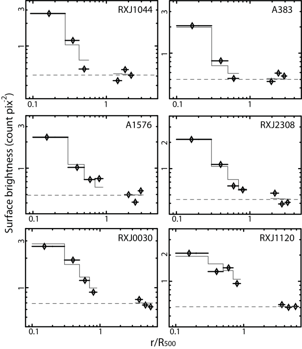
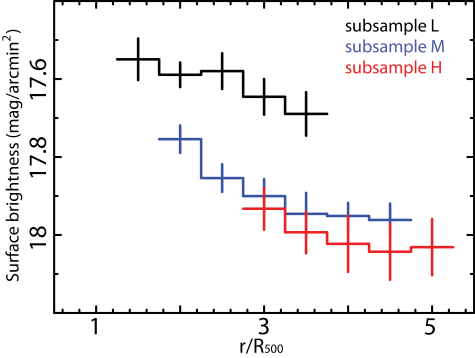
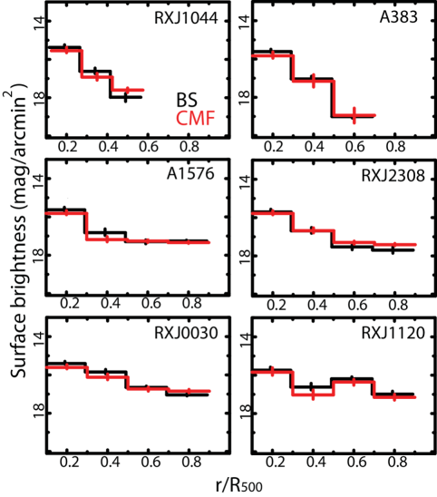
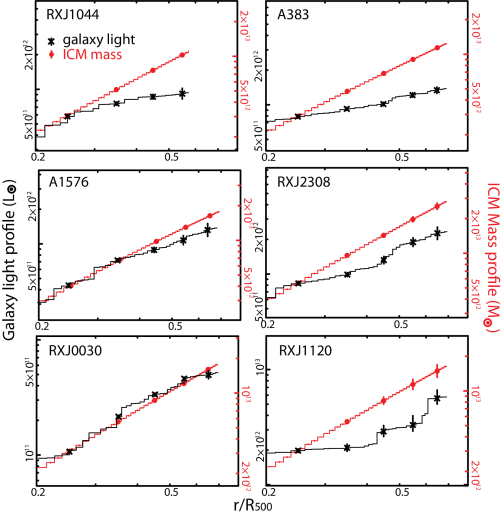
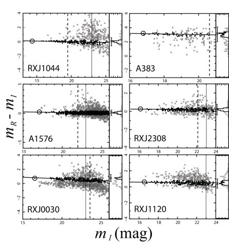
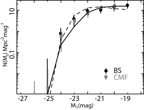
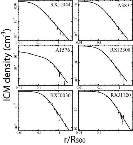
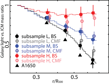
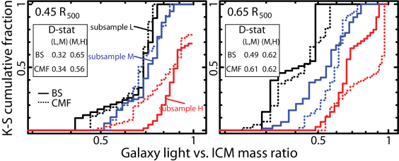
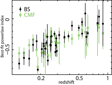
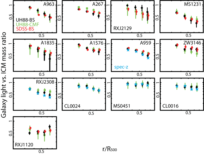
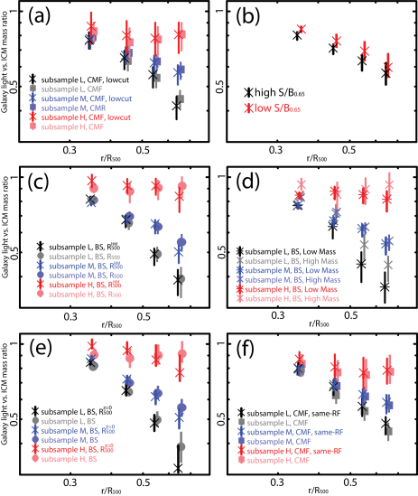
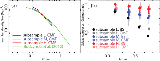

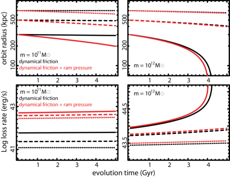
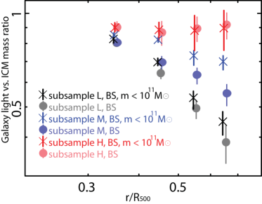
Appendix A Individual cluster profiles