Entangled state engineering of vibrational modes in a multi-membrane optomechanical system

Abstract

We propose a method to generate entangled states of the vibrational modes of $N$ membranes which are coupled to a cavity mode via the radiation pressure. Using sideband excitations, we show that arbitrary entangled states of vibrational modes of different membranes can be produced in principle by sequentially applying a series of classical pulses with desired frequencies, phases and durations. As examples, we show how to synthesize several typical entangled states, for example, Bell states, NOON states, GHZ states and W states. The environmental effect, information leakage, and experimental feasibility are briefly discussed. Our proposal can also be applied to other experimental setups of optomechanical systems, in which many mechanical resonators are coupled to a common sing-mode cavity field via the radiation pressure.

I Introduction

Entanglement is one of the most important resources for quantum information processing Nielsen . Entanglement of the internal freedoms of microscopic systems has already been prepared experimentally Raimond , for example, the polarizations of photons Kwiat , the electronic states of atoms Hagley and spin states of ions Sackett . The entangled states in macroscopic superconducting quantum systems have been experimentally demonstrated Martinis ; Schoelkopf . Recently, the quantum properties of the mechanically vibrational modes are extensively studied from external degrees of freedom of microscopic particles (e.g., trapped ions  Wineland2011 ) to macroscopic objects physrep .

The entanglement generation and arbitrary quantum state preparation of vibrational modes in microscopic systems (e.g.,trapped ions) have been studied in both experiments and theories (e.g., see Refs. Leibfried2003 ; PhysRep ; SBZheng ; LFWei ). Thus we would like to know whether the entanglement can be generated in the systems of macroscopic mechanical resonators. The research on the coupling between superconducting quantum devices and macroscopic mechanical resonators shows that arbitrary phonon states can be produced in principle by using a proposed method liuEuroph when a macroscopic mechanical resonator is coupled to a superconducting qubits OConnell , also the generation of the squeezed and entangled states of two vibrational modes has been proposed by coupling two macroscopic mechanical resonators to the superconducting quantum devices feixue . However, their experimental realizations are still very challenge. The main obstacle is whether the macroscopic mechanical resonator can be in its ground state.

The ground state cooling Gigan ; Arcizet ; Schliesser ; Wilson-Rae ; MarquardtPRL ; TeufelPRL ; Thompson ; Schliesser2008 ; Rocheleau ; Groblacher2009 ; Park ; Schliesser2009 ; Teufel475 ; Chan2009 ; Verhagen ; jqliao of the macroscopic mechanical resonators has been theoretically studied and experimentally demonstrated by coupling them to a cavity field via the radiation pressure. Thus the optomichanical systems (see, reviews Kippenberg ; Marquardt ) provide a very good platform to study quantum mechanics at the macroscopic scale. The stationary entanglement between mechanical and cavity modes in the optomechanical systems has been studied Genes ; Vitali07PRL ; Vitali07PRA ; AMari ; HXMiao12 , and such continuous variable entanglement can be used to implement quantum teleportation LTian06 ; SGHofer ; SBarzanjeh12 . Also both tripartite and bipartite entanglement between mechanical modes and other degrees of freedom can be generated in the optomechanical systems yingdan ; tianlin ; MPaternostro07 ; CGenesNJP08 ; CGenes08 ; AXuereb12 ; MAbdi12 or the hybrid optomechanical systems with an atomic ensemble Genes2008 ; Ian2008 ; DeChiara2011 ; Genes2011 ; LZhou11 ; LHSun ; BRogers ; KHammerer09 ; huijing ; yuechang or a single-atom MWallquist10 ; Barzanjeh11 inside the cavity. Moreover, the cavity field mediated entanglement between two macroscopic mechanical resonators in the steady state  Mancini2002 ; SPirandola06 ; Hartmann2008 ; Ludwig10 ; MBhattacharya08 ; MSchmidtNJP12 ; GVacantiNJP08 ; KBorkje11 ; LMazzola11 ; CJoshi12 ; MAbdiPRL12 has also been theoretically explored. However, the coherent engineering of arbitrarily entangled phonon states of the macroscopic mechanical resonators is still an open question.

We have studied a deterministic method, which is different from the proposals on measurement-based on phonon state generation pepper ; kim , to synthesize arbitrary nonclassical phonon states in optomechanical systems Xu_Liu . Recent studies show that many macroscopic mechanical resonators can be coupled to a common single-mode cavity field M1 ; M2 ; Tomadin ; Xuereb ; Schmidt ; holmes ; Seok ; Massel via the radiation pressure, which has been theoretically studied for selected entanglement generation Schmidt , synchronization holmes and mechanical analogue of nonlinear quantum optics Seok of many mechanical modes, and also experimentally demonstrated tripartite mixing for one cavity mode and two mechanical mode in the system that a microwave cavity is coupled to two and more mechanical resonators Massel . In such system, the single-mode cavity field is a very good candidate to act as a data bus for information transfer from one mechanical mode to another one. Motivated by those researches, we use a multiple membrane optomechanical system M1 ; M2 ; Tomadin ; Xuereb as an example to study entangled phonon state engineering, in optomechanical systems with the many mechanical resonators coupled to a single-mode cavity field, by using the sideband excitations and and the single-photon effect jqliao1 induced by the photon blockade. In particular, we will study detailed steps on engineering several typical entangled phonon states.

The paper is organized as follows. In Sec. II, the theoretical model of the optomechanical system with multiple membranes inside a single-mode cavity is introduced. In Sec. III, we study a method to generate entangled states for the system parameters within so-called Lamb-Dicke approximation. As examples, we show how to generate Bell, NOON, GHZ and W states. In Sec. IV, we study entangled state engineering beyond the Lamb-Dicke approximation for the strong single-photon optomechanical coupling. Finally, discussions on experimental feasibility and conclusions are given in Sec. V.

II Theoretical model

II.1 Mode equations and transfer matrix theory

The mode equations of optomechanical systems with one and two membranes inside cavity have been studied by using the boundary conditions and the Helmholtz equations M1 ; M2 ; Hartmann2008 . However, the mode equations become harder and harder to be solved with the increase of the membrane number. The transfer-matrix method has been used widely in optics to analyze the propagation of electromagnetic fields especially in multi-layer structures Born . It has been used to study the scattering problems in optomechanical systems Xuereb1 ; Xuereb2 ; Horsley . For the completeness of the paper, we will first derive intrinsic mode equations of the optomechanical systems with $N$ membranes inside a cavity using the transfer-matrix method.

As a schematic diagram in Fig. 1, we focus on an optomechanical system with a cavity containing $N$ non-absorptive membranes, that each has reflection coefficient $R$, mass $M_{i}$, position $q_{i}$, and vibration frequency $\omega_{i}$ ($i=1,\cdots,N$). We assume that the thickness of each vibrational membrane is much smaller than the wave length of the cavity mode, so the electric susceptibility in the cavity can be approximatively described by a sum of the dielectric permittivity with $\delta$ functions Spencer1972 ; Fader1985

$$\varepsilon\left(x\right)=\varepsilon_{0}\left(1+\frac{\zeta}{k}\sum_{i=1}^{N}\delta\left(x-q_{i}\right)\right),$$ (1)

where $\varepsilon_{0}$ is the dielectric permittivity of vacuum, $\zeta=2\sqrt{R/(1-R)}$, and $k=\omega/c$ is the wave vector of the electric field with the mode frequency $\omega$ and the speed $c$ of light in vacuum.

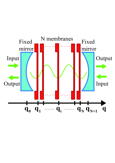
Figure 1: Schematic diagram of an optomechanical system with $N$ mechanical membranes inside the cavity which is driven by a classical field. Here, the two mirrors of the cavity are fixed. $q_{0}$ and $q_{N+1}$ denote the positions of the cavity mirrors, $q_{1},\cdots,q_{i},\cdots,q_{N}$ denote the positions of the $N$ membranes.

It is well known that the transfer matrix describing the electric field through the empty space of length $l$ is given by Born

$$M\left(k,l\right)=\left(\begin{array}[]{cc}\cos kl&\frac{1}{k}\sin kl\\ -k\sin kl&\cos kl\end{array}\right).$$ (2)

Let us now study the transfer matrix of the whole system by exploring the properties of the electric fields cross a membrane. The continuity of $E\left(x\right)$ at the position of the $i$th membrane (e.g. $x=q_{i}$) is give as

$$E\left(q_{i}^{+}\right)=E\left(q_{i}^{-}\right),$$ (3)

where $E\left(q_{i}^{-}\right)$ and $E\left(q_{i}^{+}\right)$ are the notations of the left- and right-hand limits of $E\left(x\right)$ when $x$ approaches $q_{i}$. Using the Helmholtz equations, $E^{\prime\prime}\left(x\right)=-\omega^{2}\mu_{0}\varepsilon\left(x\right)E\left(x\right)$, the derivative relations of $E(x)$ in the left- and right-hand of the $i$th membrane at the position $q_{i}$ is given as

$$E^{\prime}\left(q_{i}^{+}\right)=E^{\prime}\left(q_{i}^{-}\right)-k\zeta E\left(q_{i}\right),$$ (4)

with $E^{\prime}\left(x\right)=dE\left(x\right)/dx$. Eqs. (3) and (4) can be written in a matrix form as

$$\left(\begin{array}[]{c}E\left(q_{i}^{+}\right)\\ E^{\prime}\left(q_{i}^{+}\right)\end{array}\right)=Q\left(k,\zeta\right)\left(\begin{array}[]{c}E\left(q_{i}^{-}\right)\\ E^{\prime}\left(q_{i}^{-}\right)\end{array}\right),$$ (5)

where

$$Q\left(k,\zeta\right)=\left(\begin{array}[]{cc}1&0\\ -k\zeta&1\end{array}\right)$$ (6)

is the transfer matrix of the electric field through the $i$th membrane. Using Eq. (2) and (5), the relation of the electric fields at the left and right mirrors can be given by

$$\left(\begin{array}[]{c}E\left(q_{N+1}\right)\\ E^{\prime}\left(q_{N+1}\right)\end{array}\right)=X_{N}\left(\begin{array}[]{c}E\left(q_{0}\right)\\ E^{\prime}\left(q_{0}\right)\end{array}\right),$$ (7)

with the transfer matrix

$$X_{N} = \left(\begin{array}[]{cc}x_{11}&x_{12}\\ x_{21}&x_{22}\end{array}\right)$$

$$= \prod_{i=1}^{N}\left[M\left(k,q_{i+1}-q_{i}\right)Q\left(k,\zeta\right)\right]M\left(k,q_{1}-q_{0}\right).$$

Eq. (7) can be rewritten as

$$E\left(q_{N+1}\right) = x_{11}E\left(q_{0}\right)+x_{12}E^{\prime}\left(q_{0}\right),$$ (11)

$$E^{\prime}\left(q_{N+1}\right) = x_{21}E\left(q_{0}\right)+x_{22}E^{\prime}\left(q_{0}\right).$$ (12)

If we assume that the electric field satisfies the standing wave boundary conditions

$$E\left(q_{0}\right)=E\left(q_{N+1}\right)=0,$$ (13)

then we obtain the intrinsic mode equation

$$x_{12}\left(k,q_{0},q_{1},\cdots,q_{N+1}\right)=0.$$ (14)

We further study the intrinsic mode equation in Eq. (14) by several concrete examples. For $N=1$, the wave vector $k$ obeys the intrinsic mode equation

$$C_{1,0}+\zeta C_{1,1}=0,$$ (15)

with

$$C_{1,0} = \sin k\left(q_{2}-q_{0}\right),$$

$$C_{1,1} = \sin k\left(q_{1}-q_{2}\right)\sin k\left(q_{1}-q_{0}\right).$$

For $N=2$, the intrinsic mode equation for $k$ is

$$C_{2,0}+\zeta C_{2,1}+\zeta^{2}C_{2,2}=0,$$ (16)

with

$$C_{2,0} = \sin k\left(q_{3}-q_{0}\right),$$

$$C_{2,1} = \sin k\left(q_{1}-q_{0}\right)\sin k\left(q_{1}-q_{3}\right),$$

$$+\sin k\left(q_{2}-q_{0}\right)\sin k\left(q_{2}-q_{3}\right),$$

$$C_{2,2} = \sin k\left(q_{1}-q_{0}\right)\sin k\left(q_{2}-q_{1}\right)\sin k\left(q_{3}-q_{2}\right).$$

If there are $N$ membranes inside the cavity, the wave vector $k$ obeys the following equation

$$\sum_{i=0}^{N}\zeta^{i}C_{N,i}=0,$$ (17)

where $C_{N,i}$ are functions of the $q_{i}$, $i=0,1,2,\cdots,N+1$.

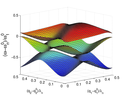
Figure 2: The frequency shift of the intrinsic optical modes $(\omega-\omega_{n}^{0})/\omega_{1}^{0}$ for two membranes in the cavity as function of displacements of the membranes, $(q_{1}-q_{1}^{0})/\lambda_{n}$ and $(q_{2}-q_{2}^{0})/\lambda_{n}$, where $\lambda_{n}=2L/n$, $\omega_{1}^{0}=\pi c/L$, $\omega_{n}^{0}=n\pi c/L$, $q_{3}-q_{2}^{0}=q_{2}^{0}-q_{1}^{0}=q_{1}^{0}-q_{0}=L$. The parameters are $R=0.7$, $n=10^{5}$.

The frequency dependence of the cavity modes $\omega\left(\left\{q_{i}\right\}\right)$ on the positions of the $N$ membranes can be obtained by solving the intrinsic mode equation in Eq. (14) numerically or analytically by using perturbation theory. Here, $\{q_{i}\}$ is an abbreviation of $\{q_{1},\cdots,q_{i},\cdots,q_{N}\}$ for the set of the positions of the membranes. For example, in Fig. 2, several intrinsic mode frequencies have been numerically simulated and plotted as functions of the displacements of the membranes when there are two vibrating membranes inside the cavity. Analytically, the frequencies of the cavity modes can be given as

$$\omega\left(\left\{q_{i}\right\}\right) = \omega\left(\left\{q_{i}^{0}\right\}\right)+\underset{i=1}{\overset{N}{\sum}}g_{i}^{(1)}\left(q_{i}-q_{i}^{0}\right)$$

$$+\underset{i,j=1}{\overset{N}{\sum}}g_{i,j}^{(2)}\left(q_{i}-q_{i}^{0}\right)\left(q_{j}-q_{j}^{0}\right)+\cdots,$$

under the condition $(q_{i}-q_{i}^{0})/\lambda\ll 1$, where

$$g_{i}^{(1)} = \left[\frac{\partial\omega\left(\left\{q_{i}\right\}\right)}{\partial q_{i}}\right]_{\left\{q_{i}=q_{i}^{0}\right\}},$$ (19)

$$g_{i,j}^{(2)} = \frac{1}{2}\left[\frac{\partial^{2}\omega\left(\left\{q_{i}\right\}\right)}{\partial q_{i}\partial q_{j}}\right]_{\left\{q_{i}=q_{i}^{0},q_{j}=q_{j}^{0}\right\}},$$ (20)

$\lambda$ is the wave length of optical mode, and $q_{i}^{0}$ ($i=1,\cdots,N$) is the position of the $i$th membrane when there is no radiation pressure.

II.2 Hamiltonian of the system

Based on above discussions, the Hamiltonian of the optomechanical system with $N$ membranes inside the cavity can be written as Law1995

$$H=\hbar\omega\left(\left\{q_{i}\right\}\right)a^{{\dagger}}a+\underset{i=1}{\overset{N}{\sum}}\left[\frac{p_{i}^{2}}{2M_{i}}+\frac{1}{2}M_{i}\omega_{i}^{2}\left(q_{i}-q_{i}^{0}\right)^{2}\right],$$ (21)

where $a$ ($a^{\dagger}$) is the annihilation (creation) operator of the cavity field, $p_{i}$ is the momentum of the $i$th vibrational membrane. Substituting Eq. (II.1) into Eq. (21), we have

$$H = \hbar\omega\left(\left\{q_{i}^{0}\right\}\right)a^{{\dagger}}a+\underset{i=1}{\overset{N}{\sum}}\left[\frac{p_{i}^{2}}{2M_{i}}+\frac{1}{2}M_{i}\omega_{i}^{2}\left(q_{i}-q_{i}^{0}\right)^{2}\right]$$

$$+\hbar a^{{\dagger}}a\underset{i=1}{\overset{N}{\sum}}g_{i}^{(1)}\left(q_{i}-q_{i}^{0}\right)$$

$$+\hbar a^{{\dagger}}a\underset{i,j=1}{\overset{N}{\sum}}g_{i,j}^{(2)}\left(q_{i}-q_{i}^{0}\right)\left(q_{j}-q_{j}^{0}\right)+\cdots.$$

The third and fourth term are the linear and quadratic interactions between the cavity mode and the vibrational modes of the membranes.

Hereafter, we only consider that the frequency shift of the cavity mode is linearly dependent on the membranes’ displacements. We also assume that the cavity is driven by an external field with the frequency $\omega_{d}$ and the phase $\phi_{d}$. Thus, we have the Hamiltonian of the driven system as below

$$H_{d} = \hbar\omega_{a}a^{{\dagger}}a+\underset{i=1}{\overset{N}{\sum}}\hbar\omega_{i}b_{i}^{{\dagger}}b_{i}+\hbar a^{{\dagger}}a\sum_{i=1}^{N}g_{i}\left(b_{i}^{{\dagger}}+b_{i}\right)$$ (23)

$$+\hbar\Omega\left[a^{{\dagger}}e^{-i\left(\omega_{d}t+\phi_{d}\right)}+ae^{i\left(\omega_{d}t+\phi_{d}\right)}\right].$$

$\Omega$ denotes the Rabi frequency of the driven field. We assume that both the frequency $\omega_{d}$ and the phase $\phi_{d}$ are controllable parameters such that they can be chosen as different values in the steps of the state preparation described below. For the simplicity, the frequency of the cavity mode is denoted as $\omega_{a}\equiv\omega\left(\left\{q_{i}^{0}\right\}\right)$, and the coupling strength between the cavity field and the $i$th membrane is simply written as $g_{i}$. The operators of the membranes are rewritten by the annihilation and creation operators $b_{i}=\sqrt{M_{i}\omega_{i}/2\hbar}(q_{i}-q_{i}^{0})+ip_{i}/\sqrt{2\hbar M_{i}\omega_{i}}$ and $b_{i}^{\dagger}=\sqrt{M_{i}\omega_{i}/2\hbar}(q_{i}-q_{i}^{0})-ip_{i}/\sqrt{2\hbar M_{i}\omega_{i}}$. We now applying a unitary transformation to Eq. (23)

$$U=\exp\left(a^{{\dagger}}a\underset{i=1}{\overset{N}{\sum}}\left[\frac{g_{i}}{\omega_{i}}\left(b_{i}^{{\dagger}}-b_{i}\right)\right]\right),$$ (24)

then the Hamiltonian in Eq. (23) becomes into

$$H_{\rm eff} = \hbar(\omega_{a}-\Delta_{0}a^{{\dagger}}a)a^{{\dagger}}a+\hbar\underset{i=1}{\overset{N}{\sum}}\omega_{i}b_{i}^{{\dagger}}b_{i}$$

$$+ \hbar\Omega a^{{\dagger}}\exp\left[{\underset{i=1}{\overset{N}{\sum}}\eta_{i}\left(b_{i}^{{\dagger}}-b_{i}\right)-i\left(\omega_{d}t+\phi_{d}\right)}\right]+\rm{H.c.},$$

where $\Delta_{0}={\sum}^{N}_{i=1}(g_{i}^{2}/\omega_{i})$ characterizes the nonlinearity of the cavity field induced by the vibrational membranes, thus the nonlinearity increases with the increase of the number of the membranes. We call $\eta_{i}=g_{i}/\omega_{i}$ as the Lamb-Dicke parameter in analog to the trapped ions Leibfried2003 . Both the strong optomechanical coupling and many mechanical resonator make the nonlinear term $\Delta_{0}$ guarantee the photon blockade, in this case, the driving field can be assumed to be coupled to two lowest energy levels $\left|0\right\rangle$ and $\left|1\right\rangle$ of the cavity field. Thus, the cavity field is confined to the states $|0\rangle$ and $|1\rangle$, and the Hamiltonian in Eq. (II.2) becomes into

$$H_{\rm two} = \hbar\frac{\omega_{0}}{2}\sigma_{z}+\hbar\sum_{i=1}^{N}\omega_{i}b_{i}^{{\dagger}}b_{i}$$

$$+ \hbar\Omega\sigma_{+}\exp\left[\sum_{i=1}^{N}\eta_{i}(b_{i}^{{\dagger}}-b_{i})-i\left(\omega_{d}t+\phi_{d}\right)\right]+{\rm H.c.},$$

by using the operators $\sigma_{z}=\left|1\right\rangle\left\langle 1\right|-\left|0\right\rangle\left\langle 0\right|$ and $\sigma_{+}=\left|1\right\rangle\left\langle 0\right|$. Here, $\omega_{0}=\omega_{a}-\Delta_{0}$. Hereafter, we denote the photon number states as $\left|1\right\rangle\equiv\left|e\right\rangle$, $\left|0\right\rangle\equiv\left|g\right\rangle$. The Hamiltonian in Eq. (II.2) can be further written as

$$H_{\rm two}=H_{0}+H_{\rm int},$$ (27)

with

$$H_{0}=\hbar\frac{\omega_{0}}{2}\sigma_{z}+\sum_{i=1}^{N}\hbar\omega_{i}b_{i}^{{\dagger}}b_{i},$$ (28)

and

$$H_{\rm int} = \hbar\Omega\sigma_{+}e^{-i\left(\omega_{d}t+\phi_{d}\right)}\prod_{i=1}^{N}\left[e^{-\frac{1}{2}\eta_{i}^{2}}\sum_{j_{i},k_{i}=0}^{+\infty}\frac{\left(-1\right)^{k_{i}}\eta_{i}^{j_{i}+k_{i}}}{j_{i}!k_{i}!}\right.$$ (29)

$$\left.\times b_{i}^{{\dagger}j_{i}}b_{i}^{k_{i}}\right]+{\rm H.c.}.$$

From Eq. (29), we find that $|k_{i}-j_{i}|$ phonons can be created ($k_{i}>j_{i}$) or annihilated ($k_{i}<j_{i}$) from the $i$th membrane when one photon is annihilated in the cavity with the assistance of the external field. Below, we will show entangled state engineering for different vibrational modes of the membranes for two cases with or without Lamb-Dicke approximation.

III Engineering entangled states with Lamb-Dicke approximation

We first study the entanglement engineering under the Lamb-Dicke approximation condition $g_{i}/\omega_{i}\ll 1$ as for the trapped ion case Leibfried2003 , thus the Hamiltonian in Eq. (29) can be written as

$$H_{\rm int}=\hbar\Omega\sigma_{+}e^{-i\left(\omega_{d}t+\phi_{d}\right)}\left[1+\sum_{i=1}^{N}\eta_{i}\left(b_{i}^{{\dagger}}-b_{i}\right)\right]+{\rm H.c.},$$ (30)

up to the first order of $\eta_{i}$. In the interaction picture with $V=\exp(iH_{0}t/\hbar)H_{\rm int}\exp(-iH_{0}t/\hbar)$, we have

$$V = \hbar\Omega\sigma_{+}e^{-i\phi_{d}}\left[e^{-i\Delta_{c}t}+\sum_{i=1}^{N}\eta_{i}\left(b_{i}^{{\dagger}}e^{-i\Delta_{b}^{i}t}-b_{i}e^{-i\Delta_{r}^{i}t}\right)\right]$$ (31)

$$+{\rm H.c.},$$

with $\Delta_{c}=\omega_{d}-\omega_{0}$, $\Delta_{b}^{i}=\omega_{d}-\omega_{0}-\omega_{i}$, and $\Delta_{r}^{i}=\omega_{d}-\omega_{0}+\omega_{i}$. If the system satisfies the resonant condition either $\Delta_{c}=0$ or $\Delta_{b}^{i}=0$ or $\Delta_{r}^{i}=0$, and also the driving field is not very strong, then we have

$$V=\hbar\Omega\times\left\{\begin{array}[]{ll}\sigma_{+}e^{-i\phi_{c}}+{\rm H.c.}&\omega_{d}=\omega_{0},\\ \eta_{i}\sigma_{+}b_{i}^{{\dagger}}e^{-i\phi_{b}^{i}}+{\rm H.c.}&\omega_{d}=\omega_{0}+\omega_{i},\\ \eta_{i}\sigma_{+}b_{i}e^{-i\phi_{r}^{i}}+{\rm H.c.}&\omega_{d}=\omega_{0}-\omega_{i}.\end{array}\right.$$ (32)

with the rotating wave approximation. For convenience, the minus sign before $\eta_{i}\sigma_{+}b_{i}e^{-i\phi_{r}^{i}}$ is absorbed by the phase $\phi_{r}^{i}$.

III.1 The time evolution operators

From the Schrödinger equation, the wave function of the system at the time $t$ can be written as

$$\left|\psi\left(t\right)\right\rangle=U\left(t\right)\left|\psi\left(0\right)\right\rangle,$$ (33)

where $U\left(t\right)=\exp\left(-iVt/\hbar\right)$ is the time evolution operator LFWei . By using the completeness relation

$$\sum_{\left\{m_{j}\right\}=0}^{+\infty}\sum_{s=g}^{e}\left|s,\left\{m_{j}\right\}\right\rangle\left\langle s,\left\{m_{j}\right\}\right|=I,$$ (34)

the time evolution operator can be written as

$$U\left(t\right)=\sum_{\left\{m_{j}\right\}=0}^{+\infty}\sum_{s=g}^{e}U\left(t\right)\left|s,\left\{m_{j}\right\}\right\rangle\left\langle s,\left\{m_{j}\right\}\right|,$$ (35)

where $|\{m_{i}\}\rangle$ is an abbreviation of the state $|m_{1}\rangle\otimes\cdots\otimes|m_{i}\rangle\otimes\cdots\otimes|m_{N}\rangle\equiv|m_{1},\cdots,m_{N}\rangle$ for $N$ membranes. Here $\left|s,\left\{m_{j}\right\}\right\rangle$ implies that the cavity field is in the state $s$ ($s=e$ or $s=g$) and there are $m_{j}$ phonons in the $j$th membranes. $\{m_{j}\}$ denotes a number series, that is, $\{m_{j}\}\equiv m_{1},m_{2},\cdots,m_{N}$.

If the frequency of the driving field is resonant with the red-sideband excitation corresponding to the frequency of the $i$th membrane, i.e., $\omega_{d}=\omega_{0}-\omega_{i}$, then the Hamiltonian in Eq. (32) becomes

$$V_{m_{i}}^{i,r}=\hbar\Omega\eta_{i}\sigma_{+}b_{i}e^{-i\phi_{r}^{i}}+{\rm H.c.}.$$ (36)

In this case, the time evolution operator is given as

$$U_{m_{i}}^{i,r}\left(t\right)=\sum_{m_{i}=0}^{+\infty}\widetilde{U}_{m_{i}}^{i,r}\left(t\right)\sum_{\left\{m_{j}\right\}=0}^{+\infty}\left(\left|\left\{m_{j}\right\}\right\rangle\left\langle\left\{m_{j}\right\}\right|\right)_{j\neq i},$$ (37)

where

$$\widetilde{U}_{m_{i}}^{i,r}\left(t\right) = \cos\left(\Omega_{m_{i}}^{i}t\right)\left|g,m_{i}\right\rangle\left\langle g,m_{i}\right|$$ (38)

$$-ie^{-i\phi_{r}^{i}}\sin\left(\Omega_{m_{i}}^{i}t\right)\left|e,m_{i}-1\right\rangle\left\langle g,m_{i}\right|$$

$$+\cos\left(\Omega_{m_{i}+1}^{i}t\right)\left|e,m_{i}\right\rangle\left\langle e,m_{i}\right|$$

$$-ie^{i\phi_{r}^{i}}\sin\left(\Omega_{m_{i}+1}^{i}t\right)\left|g,m_{i}+1\right\rangle\left\langle e,m_{i}\right|$$

with the Rabi frequencies

$$\Omega_{m_{i}}^{i}=\Omega\eta_{i}\sqrt{m_{i}}\,,\;\;\;\;\;\Omega_{m_{i}+1}^{i}=\Omega\eta_{i}\sqrt{m_{i}+1}.$$ (39)

When the frequency of the driving field is resonant with the blue-sideband excitation corresponding to the frequency of the $i$th membrane, i.e., $\omega_{d}=\omega_{0}+\omega_{i}$, the Hamiltonian in Eq. (32) becomes

$$V_{m_{i}}^{i,b}=\hbar\Omega\eta_{i}\sigma_{+}b_{i}^{{\dagger}}e^{-i\phi_{b}^{i}}+{\rm H.c.}.$$ (40)

The time evolution operator of the blue-sideband excitation is

$$U_{m_{i}}^{i,b}\left(t\right)=\sum_{m_{i}=0}^{+\infty}\widetilde{U}_{m_{i}}^{i,b}\left(t\right)\sum_{\left\{m_{j}\right\}=0}^{+\infty}\left(\left|\left\{m_{j}\right\}\right\rangle\left\langle\left\{m_{j}\right\}\right|\right)_{j\neq i}$$ (41)

with

$$\widetilde{U}_{m_{i}}^{i,b}\left(t\right) = \cos\left(\Omega_{m_{i}+1}^{i}t\right)\left|g,m_{i}\right\rangle\left\langle g,m_{i}\right|$$ (42)

$$-ie^{-i\phi_{b}^{i}}\sin\left(\Omega_{m_{i}+1}^{i}t\right)\left|e,m_{i}+1\right\rangle\left\langle g,m_{i}\right|$$

$$+\cos\left(\Omega_{m_{i}}^{i}t\right)\left|e,m_{i}\right\rangle\left\langle e,m_{i}\right|\left\langle e,m_{i}\right|$$

$$-ie^{i\phi_{b}^{i}}\sin\left(\Omega_{m_{i}}^{i}t\right)\left|g,m_{i}-1\right\rangle\left\langle e,m_{i}\right|.$$

Finally, if the cavity is driven by the classical field with the frequency $\omega_{d}=\omega_{0}$, then the carrier process is switched on, and the Hamiltonian in Eq. (32) is given as

$$V^{c}=\hbar\Omega\sigma_{+}e^{-i\phi_{c}}+{\rm H.c.}.$$ (43)

The time evolution operator of the carrier process is given as

$$U^{c}\left(t\right)=\widetilde{U}^{c}\left(t\right)\sum_{\left\{m_{j}\right\}=0}^{+\infty}\left|\left\{m_{j}\right\}\right\rangle\left\langle\left\{m_{j}\right\}\right|$$ (44)

and

$$\widetilde{U}^{c}\left(t\right) = \left[\cos\left(\Omega t\right)\left|g\right\rangle-ie^{-i\phi_{c}}\sin\left(\Omega t\right)\left|e\right\rangle\right]\left\langle g\right|$$ (45)

$$+\left[\cos\left(\Omega t\right)\left|e\right\rangle-ie^{i\phi_{c}}\sin\left(\Omega t\right)\left|g\right\rangle\right]\left\langle e\right|.$$

Based on above three different processes, we can in principle engineer any kind of entangled phonon states. However, below we will only show the engineering of several typical entangled phonon states by controlling the evolution time and the frequency of the classical driving field.

III.2 Generation of Bell and NOON states of two mechanical modes

In this section, we study the generation of entangled phonon states

$$\left|\varphi\right\rangle=\frac{1}{\sqrt{2}}\left(\left|N,0\right\rangle+\left|0,N\right\rangle\right),$$ (46)

of two vibrational modes when there are two membranes inside the cavity. Here $\left|\varphi\right\rangle$ denotes the Bell state when $N=1$. However $\left|\varphi\right\rangle$ with $N\geq 2$ represents the NOON state which plays an important role in quantum metrology Bollinger . $|N,0\rangle$ means $N$ phonons in mode one and zero phonon in mode two. Our state generation below starts from the initial state $\left|\psi\left(t_{0}\right)\right\rangle=\left|g,0,0\right\rangle$ of the whole system.

We now show how to generate a Bell state. First, a driving field satisfying the carrier process is applied to the cavity, then after the interaction time $\Delta t_{1}=\pi/2\Omega$, the system state at the time $t_{1}=t_{0}+\Delta t_{1}$ is

$$\left|\psi\left(t_{1}\right)\right\rangle=\left|e,0,0\right\rangle,$$ (47)

here a global phase has been neglected. Second, the frequency of the driving field is turned to the red sideband corresponding to the frequency of the first membrane, i.e., $\omega_{d}=\omega_{0}-\omega_{1}$. With an evolution time $\Delta t_{2}$, the system evolves to

$$\left|\psi\left(t_{2}\right)\right\rangle=\left(1-\left|C_{1,0}\right|^{2}\right)^{1/2}\left|e,0,0\right\rangle+C_{1,0}\left|g,1,0\right\rangle$$ (48)

at the time $t_{2}=t_{1}+\Delta t_{2}$ with the parameter

$$C_{1,0}=-ie^{i\phi_{r}^{1}}\sin\left(\Omega_{1}^{1}\Delta t_{2}\right).$$ (49)

If the time duration and the phase of the driving field are chosen as $\Delta t_{2}=\pi/4\Omega_{1}^{1}$, phase $\phi_{r}^{1}=\pi/2$, then $C_{1,0}=1/\sqrt{2}$, and the state of the system becomes into

$$\left|\psi\left(t_{2}\right)\right\rangle=\frac{1}{\sqrt{2}}\left|e,0,0\right\rangle+\frac{1}{\sqrt{2}}\left|g,1,0\right\rangle.$$ (50)

In the third step, the frequency of the driving field is tuned to the red sideband corresponding to the frequency of the second membrane, i.e., $\omega_{d}=\omega_{0}-\omega_{2}$. With the evolution time $\Delta t_{3}$, the system evolves into

$$\left|\psi\left(t_{3}\right)\right\rangle = \frac{1}{\sqrt{2}}\left[\left(1-\left|C_{0,1}\right|^{2}\right)^{1/2}\left|e,0,0\right\rangle+C_{0,1}\left|g,0,1\right\rangle\right]$$ (51)

$$+\frac{1}{\sqrt{2}}\left|g,1,0\right\rangle$$

at the time $t_{3}=t_{2}+\Delta t_{3}$ with the parameter

$$C_{0,1}=-ie^{i\phi_{r}^{2}}\sin\left(\Omega_{1}^{2}\Delta t_{3}\right).$$ (52)

If we choose the time duration $\Delta t_{3}=\pi/2\Omega_{1}^{2}$ and phase $\phi_{r}^{2}=\pi/2$, then the state of the system becomes

$$\left|\psi\left(t_{3}\right)\right\rangle=|g\rangle\otimes\frac{1}{\sqrt{2}}\left(\left|0,1\right\rangle+\left|1,0\right\rangle\right).$$ (53)

Thus the system is deterministically prepared to a product state of the Bell state of two mechanical resonators and the ground state $\left|g\right\rangle$ of the cavity field.

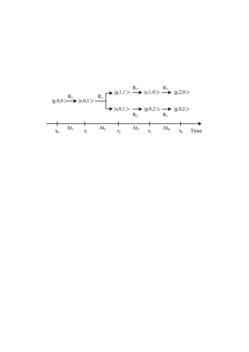
Figure 3: Schematic diagrams for preparing NOON states $\left(\left|2,0\right\rangle+\left|0,2\right\rangle\right)/\sqrt{2}$. The letters $R$, $B$ and $C$ represent the process that the driving field is tuned to the red-sideband, blue-sideband or carrier processes, respectively. Each number of the subscript denotes the sideband excitations corresponding to the frequency of the $i$th membrane.

We now describe a detailed steps for preparing an arbitrary NOON state of two vibrational membranes by the simplest example with $N=2$. First, a driving field is applied to the cavity with the blue sideband excitation corresponding to frequency of the second membrane, i.e. $\omega_{d}=\omega_{0}+\omega_{2}$, with an evolution time $\Delta t_{1}=\pi/2\Omega_{1}^{2}$ and choosing the phase $\phi_{b}^{2}=3\pi/2$, the system evolves to

$$\left|\psi\left(t_{1}\right)\right\rangle=\left|e,0,1\right\rangle$$ (54)

at the time $t_{1}=t_{0}+\Delta t_{1}$. Second, the frequency of the driving field is tuned to the red sideband excitation corresponding to the frequency of the first membrane, i.e., $\omega_{d}=\omega_{0}-\omega_{1}$. With an evolution time $\Delta t_{2}=\pi/4\Omega_{1}^{1}$ and choosing the phase $\phi_{r}^{1}=\pi/2$, the state of the system becomes

$$\left|\psi\left(t_{2}\right)\right\rangle=\frac{1}{\sqrt{2}}(\left|g,1,1\right\rangle+\left|e,0,1\right\rangle).$$ (55)

at the time $t_{2}=t_{1}+\Delta t_{2}$. Third, the frequency of the driving field is tuned to the red sideband excitation corresponding to the frequency of the second membrane, i.e., $\omega_{d}=\omega_{0}-\omega_{2}$, with the time duration $\Delta t_{3}$ satisfying

$$\sin(\Omega^{2}_{1}\Delta t_{3})=\pm 1,\sin(\Omega^{2}_{2}\Delta t_{3})=\pm 1,$$ (56)

in the infinite approximation for $\Omega^{2}_{2}/\Omega^{2}_{1}=\sqrt{2}$, which is an irrational number (see the Appendix B), the state of the whole system becomes

$$\left|\psi\left(t_{3}\right)\right\rangle=\frac{1}{\sqrt{2}}(\left|e,1,0\right\rangle+\left|g,0,2\right\rangle),$$ (57)

at the time $t_{3}=t_{2}+\Delta t_{3}$. In the last step, the driving field is tuned to the red sideband excitation corresponding to the frequency of the first membrane, i.e., $\omega_{d}=\omega_{0}-\omega_{1}$. With an evolution time $\Delta t_{4}=\pi/2\Omega^{1}_{2}$ and the phase $\phi_{r}^{1}=\pi/2$, the state of the system becomes

$$\left|\psi\left(t_{4}\right)\right\rangle=|g\rangle\otimes\frac{1}{\sqrt{2}}(\left|2,0\right\rangle+\left|0,2\right\rangle),$$ (58)

at the time $t_{4}=t_{3}+\Delta t_{4}$. Thus the NOON state for $N=2$ is generated with the cavity field in its ground state $\left|g\right\rangle$. We have given a schematic diagram to summary all steps for generating the NOON state with $N=2$ in Fig. 3.

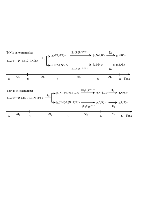
Figure 4: Schematic diagram for preparing NOON states when (I) $N$ is an even number and (II) $N$ is an odd number. The numbers in the superscript denote the times of the red sideband excitation ($R$), blue sideband excitation ($B$) and carrier process ($C$). The subscript denotes the sideband excitations corresponding to the frequency of the $i$th membrane.

By using the similar steps as for generating the NOON state with $N=2$, an arbitrary NOON state of two mechanical resonators can also be generated by using the steps schematically shown in Fig. 4. The detailed steps are summarized as below. In the step (i), by alternatively applying a series of the red-sideband excitations and carrier processes, we can prepare the state

$$\left|\psi\left(t_{1}\right)\right\rangle=\left|e,\frac{N}{2}-1,\frac{N}{2}\right\rangle$$ (59)

for the even number $N$ or

$$\left|\psi\left(t_{1}\right)\right\rangle=\left|e,\frac{N-1}{2},\frac{N-1}{2}\right\rangle$$ (60)

for the odd number $N$.

In the step (ii), for the even number $N$, the system is driven with the red-sideband process $R_{1}$ for the membrane one with the time duration $\Delta t_{2}=\pi/4\Omega_{N/2}^{1}$, then we have

$$\left|\psi\left(t_{2}\right)\right\rangle=\frac{1}{\sqrt{2}}\left(\left|g,\frac{N}{2},\frac{N}{2}\right\rangle+\left|e,\frac{N}{2}-1,\frac{N}{2}\right\rangle\right).$$ (61)

For the odd number $N$, the system is driven with the red sideband excitation $R_{2}$ for the membrane two with the time duration $\Delta t_{2}=\pi/4\Omega_{(N+1)/2}^{2}$, then we have

$$\left|\psi\left(t_{2}\right)\right\rangle=\frac{1}{\sqrt{2}}\left(\left|e,\frac{N-1}{2},\frac{N-1}{2}\right\rangle+\left|g,\frac{N-1}{2},\frac{N+1}{2}\right\rangle\right).$$ (62)

In the step (iii), for the even number $N$, we alternatively apply the driving field for $N/2$ and $(N/2)-1$ red sideband excitations for membrane two and one with the appropriate time durations, respectively, that is, an operation operator $R_{2}(R_{1}R_{2})^{N/2-1}$ is acted on the state $\left|\psi(t_{2})\right\rangle$, then we have

$$\left|\psi\left(t_{3}\right)\right\rangle=\frac{1}{\sqrt{2}}\left(\left|e,N-1,0\right\rangle+\left|g,0,N\right\rangle\right).$$ (63)

For the odd number $N$, $(N-1)/2$ red sideband excitations $R_{2}$ and $R_{1}$ are applied to the membrane two and one, respectively, then we also obtain the state shown in Eq. (63).

In the step (iv), the system is driven with the red sideband excitation $R_{1}$ for the membrane one with the time duration $\Delta t_{4}=\pi/2\Omega_{N}^{1}$, we have

$$\left|\psi\left(t_{4}\right)\right\rangle=|g\rangle\otimes\frac{1}{\sqrt{2}}\left(\left|N,0\right\rangle+\left|0,N\right\rangle\right).$$ (64)

Thus the NOON state of the two mechanical resonators is prepared with the cavity field in its ground state $\left|g\right\rangle$. We note that there is information leakage in the third step because the times to the two states $\left|e,N-1,0\right\rangle$ and $\left|g,0,N\right\rangle$ are not synchronized. The fidelity of prepared NOON states from $N=2$ to $N=20$ due to such information leakage is given in Fig. 5, which shows that some states cannot be prepared with the hundred percent. The detailed discussion about this type of information leakage is given in the Appendix B.

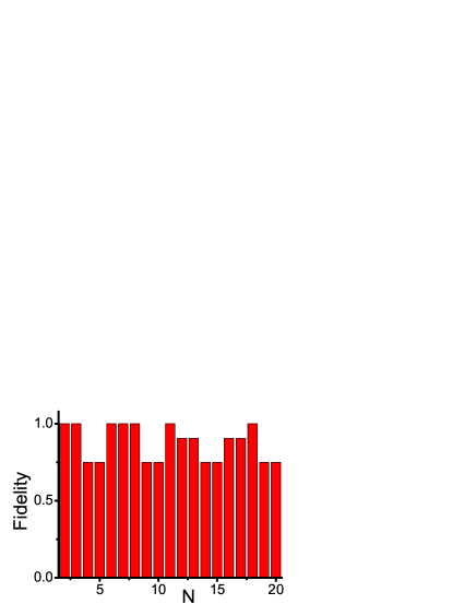
Figure 5: Fidelity for preparing NOON state $\left(\left|N,0\right\rangle+\left|0,N\right\rangle\right)/\sqrt{2}$ from $N=2$ to $N=20$.

III.3 Generating GHZ and W states of three mechanical modes

We now turn to study the generation of the Greenberger-Horne-Zeilinger (GHZ) and W states Dur2000 of three vibrational membranes inside the cavity with the initial state $\left|\psi\left(t_{0}\right)\right\rangle=\left|g,0,0,0\right\rangle$. The definitions of the GHZ state $\left|\psi\right\rangle_{\mathrm{GHZ}}$ and W state $\left|\psi\right\rangle_{\mathrm{W}}$ are

$$\left|\psi\right\rangle_{\mathrm{GHZ}}=\frac{1}{\sqrt{2}}\left(\left|0,0,0\right\rangle+\left|1,1,1\right\rangle\right).$$ (65)

and

$$\left|\psi\right\rangle_{\mathrm{W}}=\frac{1}{\sqrt{3}}\left(\left|1,0,0\right\rangle+\left|0,1,0\right\rangle+\left|0,0,1\right\rangle\right).$$ (66)

Let us first show the steps for preparing the W state. In the step (i), the cavity field is driven by a laser field with the carrier frequency. With an evolution time $\Delta t_{1}=\pi/2\Omega$ and choosing the phase $\phi_{c}=3\pi/2$, the state of the system becomes

$$\left|\psi\left(t_{1}\right)\right\rangle=\left|e,0,0,0\right\rangle.$$ (67)

In the step (ii), the frequency of the driving field is tuned to the red sideband excitation corresponding to frequency of the membrane one such that $\omega_{d}=\omega_{0}-\omega_{1}$. With the time duration $\Delta t_{2}=[\arcsin\left(1/\sqrt{3}\right)]/\Omega_{1}^{1}$ and the phase $\phi_{r}^{1}=\pi/2$, the state of the system evolves to

$$\left|\psi\left(t_{2}\right)\right\rangle=\frac{1}{\sqrt{3}}\left|g,1,0,0\right\rangle+\sqrt{\frac{2}{3}}\left|e,0,0,0\right\rangle.$$ (68)

In the step (iii), the frequency of the driving field is tuned to the red sideband excitation corresponding to the membrane two such that $\omega_{d}=\omega_{0}-\omega_{2}$. With the time duration $\Delta t_{3}=\pi/4\Omega_{1}^{2}$ and the phase $\phi_{r}^{2}=\pi/2$, the state of the system becomes

$$\left|\psi\left(t_{3}\right)\right\rangle=\frac{1}{\sqrt{3}}\left(\left|g,1,0,0\right\rangle+\left|g,0,1,0\right\rangle+\left|e,0,0,0\right\rangle\right).$$ (69)

In the step (iv), the frequency of the driving field is tuned to the red sideband excitation corresponding to the membrane three such that $\omega_{d}=\omega_{0}-\omega_{3}$. With the time duration $\Delta t_{4}=\pi/2\Omega_{1}^{3}$ and the phase $\phi_{r}^{3}=\pi/2$, the state of the system evolves to

$$\left|\psi\left(t_{4}\right)\right\rangle=|g\rangle\otimes\frac{1}{\sqrt{3}}\left(\left|1,0,0\right\rangle+\left|0,1,0\right\rangle+\left|0,0,1\right\rangle\right).$$ (70)

Thus the system is prepared in a product state of the W state of three mechanical modes and the ground state $\left|g\right\rangle$ of the cavity field.

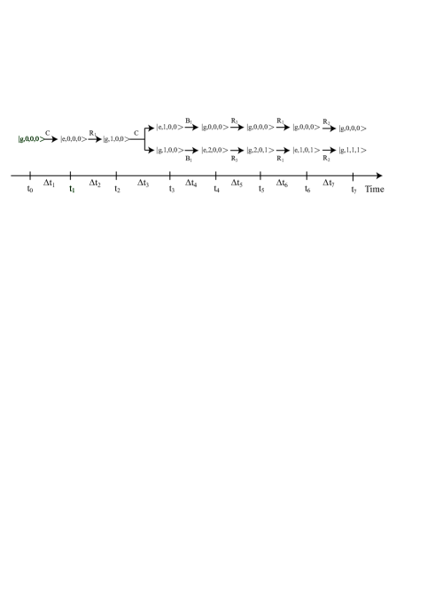
Figure 6: Schematic diagram for preparing GHZ state $\left(\left|0,0,0\right\rangle+\left|1,1,1\right\rangle\right)/\sqrt{2}$ of three mechanical resonators. The numbers in the superscript denote the times of the red sideband excitation ($R$), blue sideband excitation ($B$) and carrier process ($C$). The subscript denotes the sideband excitations corresponding to the frequency of the $i$th membrane.

Now, we are going to describe the steps of preparing the GHZ state, as schematically shown in Fig. 6. In the step (i), the cavity is driven with the carrier frequency. With the evolution time $\Delta t_{1}=\pi/2\Omega$ and the phase $\phi_{c}=3\pi/2$, the system evolves to

$$\left|\psi\left(t_{1}\right)\right\rangle=\left|e,0,0,0\right\rangle.$$ (71)

In the step (ii), the frequency of the driving field is tuned to the red sideband excitation corresponding to the membrane one such that $\omega_{d}=\omega_{0}-\omega_{1}$. With the time duration $\Delta t_{2}=\pi/2\Omega_{1}^{1}$ and the phase $\phi_{r}^{1}=\pi/2$, the state of the system evolves to

$$\left|\psi\left(t_{2}\right)\right\rangle=\left|g,1,0,0\right\rangle.$$ (72)

In the step (iii), the cavity field is driven again for the carrier process such that $\omega_{d}=\omega_{0}$. Then, with the time duration $\Delta t_{3}=\pi/4\Omega$ and the phase $\phi_{c}=3\pi/2$, the state of the system evolves to

$$\left|\psi\left(t_{3}\right)\right\rangle=\frac{1}{\sqrt{2}}\left|g,1,0,0\right\rangle+\frac{1}{\sqrt{2}}\left|e,1,0,0\right\rangle.$$ (73)

In the step (iv), the frequency of the driving field is tuned to the blue sideband excitation corresponding to the frequency of the membrane one such that $\omega_{d}=\omega_{0}+\omega_{1}$. For the time duration $\Delta t_{4}$ satisfying the condition

$$\sin(\Omega^{1}_{1}\Delta t_{4})=\pm 1,\sin(\Omega^{1}_{2}\Delta t_{4})=\pm 1,$$ (74)

with the infinite approximation (see the Appendix B), the state of the system evolves to

$$\left|\psi\left(t_{4}\right)\right\rangle=\frac{1}{\sqrt{2}}\left|g,0,0,0\right\rangle+\frac{1}{\sqrt{2}}\left|e,2,0,0\right\rangle.$$ (75)

In the step (v), the driving field to tuned to the red sideband excitation corresponding to the membrane three such that $\omega_{d}=\omega_{0}-\omega_{3}$. With the time duration $\Delta t_{5}=\pi/2\Omega_{1}^{3}$ and the phase $\phi_{b}^{3}=\pi/2$, the state of the system evolves to

$$\left|\psi\left(t_{5}\right)\right\rangle=\frac{1}{\sqrt{2}}\left|g,0,0,0\right\rangle+\frac{1}{\sqrt{2}}\left|g,2,0,1\right\rangle.$$ (76)

In the step (vi), the driving field to tuned the red sideband excitation corresponding to the membrane one such that $\omega_{d}=\omega_{0}-\omega_{1}$. With the time duration $\Delta t_{6}=\pi/2\Omega_{2}^{1}$ and the phase $\phi_{b}^{1}=3\pi/2$, the state of the system evolves to

$$\left|\psi\left(t_{6}\right)\right\rangle=\frac{1}{\sqrt{2}}\left|g,0,0,0\right\rangle+\frac{1}{\sqrt{2}}\left|e,1,0,1\right\rangle.$$ (77)

In the step (vii), the driving field is tuned to the red sideband excitation corresponding to the membrane two such that $\omega_{d}=\omega_{0}-\omega_{2}$. With the time duration $\Delta t_{7}=\pi/2\Omega_{1}^{2}$ and the phase $\phi_{b}^{1}=\pi/2$, the state of the system evolves to

$$\left|\psi\left(t_{7}\right)\right\rangle=|g\rangle\otimes\frac{1}{\sqrt{2}}\left(\left|0,0,0\right\rangle+\left|1,1,1\right\rangle\right).$$ (78)

Thus the whole system is prepared to a product state of the GHZ state of three mechanical resonators and the ground state $\left|g\right\rangle$ of the cavity field.

In principle, our method can be generalized to generation of the W and GHZ states of $N$ membranes by sequentially applying a series of red-sideband excitations, blue-sideband excitations and carrier process with well chosen the time intervals, phases of the driving field. We have shown the steps for the generation of those states in the appendix A.

IV Preparation of entangled states beyond the Lamb-Dicke approximation

In the above, we have studied a detailed method of generating entangled states in the Lamb-Dicke approximation with $\eta_{i}\ll 1$. However, in some optomechanical systems, e.g., a Bose-Einstein condensate served as the mechanical oscillator coupled to the cavity field Murch ; Brennecke , the condition $\eta_{i}\ll 1$ is not satisfied, and also with the experimental progress, the parameter $\eta_{i}$ outside the Lamb-Dicke regime is possible to be achieved in the near future in the other types of optomechanical systems. For the parameter $\eta_{i}$ outside the Lamb-Dicke approximation, the higher-order powers of the Lamb-Dicke parameter should be taken into account. We now show how to generate entangled states beyond the Lamb-Dicke approximation by using a similar but not same method given in Ref. SBZheng . Because the generation of the Bell state and the W state can use the same method as in the Lamb-Dicke approximation described in Sec. III, thus below we focus on the generation of the NOON state and the GHZ state.

Beyond the Lamb-Dicke regime by assuming $k_{i}=j_{i}+n_{i}$, the Hamiltonian in Eq. (29) can be rewritten as

$$H_{\rm int}=\hbar\Omega\sigma_{+}e^{-i\left(\omega_{d}t+\phi_{d}\right)}\prod_{i=1}^{N}e^{-\frac{1}{2}\eta_{i}^{2}}H_{i}+{\rm H.c.},$$ (79)

with

$$H_{i}=\sum_{n_{i}=-\infty}^{+\infty}\sum_{j_{i}=\max[0,-n_{i}]}^{+\infty}\frac{\alpha^{i}_{j_{i},n_{i}}\left(b_{i}^{{\dagger}}\right)^{j_{i}}\left(b_{i}\right)^{j_{i}+n_{i}}}{j_{i}!\left(j_{i}+n_{i}\right)!}$$ (80)

where $\alpha^{i}_{j_{i},n_{i}}=\left(-1\right)^{j_{i}+n_{i}}\eta_{i}^{2j_{i}+n_{i}}$. The Hamiltonian in the interaction picture is given by $V(t)=e^{iH_{0}t/\hbar}H_{\rm int}e^{-iH_{0}t/\hbar}$, thus we have

$$V(t)=\hbar\Omega\sigma_{+}e^{-i\left(\Delta_{d}t+\phi_{d}\right)}\prod_{i=1}^{N}e^{-\frac{1}{2}\eta_{i}^{2}}H_{i}(t)+{\rm H.c.},$$ (81)

with

$$H_{i}(t)=\sum_{n_{i}=-\infty}^{+\infty}\sum_{j_{i}=\max[0,-n_{i}]}^{+\infty}\frac{\alpha^{i}_{j_{i},n_{i}}\left(b_{i}^{{\dagger}}\right)^{j_{i}}\left(b_{i}\right)^{j_{i}+n_{i}}}{j_{i}!\left(j_{i}+n_{i}\right)!}e^{-in_{i}\omega_{i}t}$$ (82)

here $\Delta_{d}=\omega_{d}-\omega_{0}$. We assume that the off-resonant transitions can be neglected in the resonant or near-resonant driving condition. When the driving field satisfies the condition $\omega_{d}=\omega_{0}-\sum_{i=1}^{N}n_{i}\omega_{i}$, we have

$$V^{\left\{n_{i}\right\}}=\hbar\Omega\sigma_{+}e^{-i\phi_{d}}\prod_{i=1}^{N}e^{-\frac{1}{2}\eta_{i}^{2}}H_{i,n_{i}}+{\rm H.c.},$$ (83)

with $H_{i,n_{i}}$ given by

$$H_{i,n_{i}}=\sum_{j_{i}=\max[0,-n_{i}]}^{+\infty}\frac{\alpha^{i}_{j_{i},n_{i}}\left(b_{i}^{{\dagger}}\right)^{j_{i}}\left(b_{i}\right)^{j_{i}+n_{i}}}{j_{i}!\left(j_{i}+n_{i}\right)!},$$ (84)

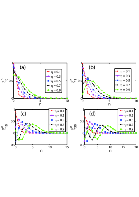
Figure 7: $\xi_{m_{i}}^{n_{i}}$ in Eq. (91) is plotted as the function of $n_{i}$ for different values of $\eta=0.1,\,0.3,\,0.5,\,0.7,\,0.9$ in (a) $m=0$; (b) $m=1$; (c) $m=10$; and (d) $m=30$. Here, for the convenience, we assume $n_{i}\equiv n$ and $m_{i}\equiv m$

With the Hamiltonian in Eq. (83) and using the completeness relation in Eq. (34), the time evolution operator can be given as

$$U^{\left\{n_{i}\right\}}\left(t\right)=\sum_{\left\{m_{i}\right\}=0}^{+\infty}U_{\left\{m_{i}\right\}}^{\left\{n_{i}\right\}}\left(t\right),$$ (85)

where

$$U_{\left\{m_{i}\right\}}^{\left\{n_{i}\right\}}\left(t\right)=\sum_{s=g}^{e}U^{\left\{n_{i}\right\}}\left(t\right)\left|s,\left\{m_{i}\right\}\right\rangle\left\langle s,\left\{m_{i}\right\}\right|.$$ (86)

Hereafter $\{n_{i}\}$ denotes a number series, that is, $\{n_{i}\}\equiv n_{1},n_{2},\cdots,n_{N}$. The operator $U_{\left\{m_{i}\right\}}^{\left\{n_{i}\right\}}\left(t\right)$ can be further written as

$$U_{\left\{m_{i}\right\}}^{\left\{n_{i}\right\}}\left(t\right) = \left(1-\left|C_{\left\{m_{i}-n_{i}\right\}}^{\left\{n_{i}\right\}}\right|^{2}\right)^{1/2}\left|g,\left\{m_{i}\right\}\right\rangle\left\langle g,\left\{m_{i}\right\}\right|$$ (87)

$$+C_{\left\{m_{i}-n_{i}\right\}}^{\left\{n_{i}\right\}}\left|e,\left\{m_{i}-n_{i}\right\}\right\rangle\left\langle g,\left\{m_{i}\right\}\right|$$

$$+\left(1-\left|\widetilde{C}_{\left\{m_{i}\right\}}^{\left\{n_{i}\right\}}\right|^{2}\right)^{1/2}\left|e,\left\{m_{i}\right\}\right\rangle\left\langle e,\left\{m_{i}\right\}\right|$$

$$+\widetilde{C}_{\left\{m_{i}\right\}}^{\left\{n_{i}\right\}}\left|g,\left\{m_{i}+n_{i}\right\}\right\rangle\left\langle e,\left\{m_{i}\right\}\right|,$$

where

$$C_{\left\{m_{i}\right\}}^{\left\{n_{i}\right\}}=-ie^{-i\phi_{d}}\left(-1\right)^{\sum_{i=1}^{N}n_{i}}\sin\left(\Omega_{\left\{m_{i}\right\}}^{\left\{n_{i}\right\}}t\right)$$ (88)

with

$$\widetilde{C}_{\left\{m_{i}\right\}}^{\left\{n_{i}\right\}}=-\left(C_{\left\{m_{i}\right\}}^{\left\{n_{i}\right\}}\right)^{\ast},$$ (89)

and the Rabi frequency

$$\Omega_{\left\{m_{i}\right\}}^{\left\{n_{i}\right\}}=\Omega\prod_{i=1}^{N}\xi_{m_{i}}^{n_{i}}.$$ (90)

If $n_{i}\geq 0$, $\xi_{m_{i}}^{n_{i}}$ is given as

$$\xi_{m_{i}}^{n_{i}}=e^{-\frac{1}{2}\eta_{i}^{2}}\eta_{i}^{n_{i}}\sqrt{\frac{m_{i}!}{\left(m_{i}+n_{i}\right)!}}L_{m_{i}}^{n_{i}}\left(\eta_{i}^{2}\right)$$ (91)

and if $-m_{i}\leq n_{i}<0$, we have

$$\xi_{m_{i}}^{n_{i}} = e^{-\frac{1}{2}\eta_{i}^{2}}(-\eta_{i})^{-n_{i}}\sqrt{\frac{\left(m_{i}+n_{i}\right)!}{m_{i}!}}L_{m_{i}+n_{i}}^{-n_{i}}\left(\eta_{i}^{2}\right)$$ (92)

$$= (-1)^{|n_{i}|}\xi_{m_{i}-|n_{i}|}^{|n_{i}|},$$

here, $L_{m_{i}}^{n_{i}}\left(\eta_{i}^{2}\right)$ is the associated Laguerre polynomials. Because $\xi_{m_{i}}^{n_{i}}$ is related to the effective Rabi frequency, thus it is plotted as a function of $n_{i}$ in Fig. 7. We find that $\xi_{m_{i}}^{n_{i}}$ decreases rapidly to the zero with the increase of $n_{i}$ when $\eta_{i}\ll 1$ thus the Lamb-Dicke approximation is valid in this regime. However, with the increase of $\eta_{i}$, $\xi_{m_{i}}^{n_{i}}$ oscillates with the increase of $n_{i}$ and finally approach to the zero. Thus if $\eta_{i}$ is beyond the Lamb-Dicke regime, the terms for $n_{i}>1$ should be taken into account and these terms will make the state preparation much easier. It should be noted that $\xi_{m_{i}}^{n_{i}}$ decreases to zero within a finite number $n_{i}$ even $\eta_{i}=0.9$. That is, there is maximum phonon number that we can create in one step even for the case that $\eta_{i}$ is beyond the Lamb-Dicke regime.

We now study the preparation of the NOON state of two mechanical resonators beyond the Lamb-Dicke regime. The time evolution operator of the system for two membranes inside the cavity can be written out from Eq. (87) by taking the subscripts and the superscripts $\{m_{i}\}\equiv m_{1},m_{2}$, $\{m_{i}\pm n_{i}\}\equiv m_{1}\pm n_{1},m_{2}\pm n_{2}$, and $\{n_{i}\}\equiv n_{1},n_{2}$. The coefficients in Eq. (88) for the case that two membranes inside the cavity are

$$C_{m_{1},m_{2}}^{n_{1},n_{2}}=-ie^{-i\phi_{d}}\left(-1\right)^{n_{1}+n_{2}}\sin\left(\Omega_{m_{1},m_{2}}^{n_{1},n_{2}}t\right)$$ (93)

with

$$\widetilde{C}_{m_{1},m_{2}}^{n_{1},n_{2}}=-\left(C_{m_{1},m_{2}}^{n_{1},n_{2}}\right)^{\ast}.$$ (94)

and the effective Rabi frequency

$$\Omega_{m_{1},m_{2}}^{n_{1},n_{2}}=\Omega\prod_{i=1}^{2}\xi_{m_{i}}^{n_{i}}.$$ (95)

Here, $\xi_{m_{i}}^{n_{i}}$ is given by Eq. (91) or Eq. (92). We assume that the system is initially in the state $\left|\psi\left(t_{0}\right)\right\rangle=\left|g,0,0\right\rangle$.

In the step (i), the cavity field is driven by the external field which satisfies the carrier process. For the phase $\phi_{d}=3\pi/2$ and the time duration $\Delta t_{1}=\pi/2\Omega_{0,0}^{0,0}$ with the evolution operator $U_{0,0}^{0,0}\left(\Delta t_{1}\right)$, the state of the system becomes

$$\left|\psi\left(t_{1}\right)\right\rangle=\left|e,0,0\right\rangle.$$ (96)

In the step (ii), the frequency of the driving field is tuned to the $N$th red sideband excitation corresponding to the frequency of the membrane one with $\Delta_{d}=-N\omega_{1}$. With the time duration $\Delta t_{2}=\pi/4\Omega_{0,0}^{N,0}$ and the phase $\phi_{d}=\pi/2+N\pi$, the state of the system evolves to

$$\left|\psi\left(t_{2}\right)\right\rangle=\frac{1}{\sqrt{2}}\left|e,0,0\right\rangle+\frac{1}{\sqrt{2}}\left|g,N,0\right\rangle.$$ (97)

In the step (iii), the frequency of the driving field is tuned to the $N$th red sideband excitation corresponding to the frequency of the membrane two such that $\Delta_{d}=-N\omega_{2}$. With the time duration $\Delta t_{3}=\pi/2\Omega_{0,0}^{0,N}$ and the phase $\phi_{d}=\pi/2+N\pi$, the state of the system evolves to

$$\left|\psi\left(t_{3}\right)\right\rangle=|g\rangle\otimes\frac{1}{\sqrt{2}}(\left|N,0\right\rangle+\left|0,N\right\rangle).$$ (98)

Thus the NOON state of two mechanical modes is prepared with the cavity field in its ground state $\left|g\right\rangle$. It is obvious that the preparation process is more efficient than the one shown in the Lamb-Dicke regime.

We now show the steps of generating the GHZ state. The time evolution operator of the three membranes inside the cavity can be easily given from Eq. (87) by taking the subscripts and the superscripts as $\{m_{i}\}\equiv m_{1},m_{2},m_{3}$, $\{m_{i}\pm n_{i}\}\equiv m_{1}\pm n_{1},m_{2}\pm n_{2},m_{3}\pm n_{3}$, and $\{n_{i}\}\equiv n_{1},n_{2},n_{3}$. The coefficients in Eq. (88) for the case of the three membranes are given as

$$C_{m_{1},m_{2},m_{3}}^{n_{1},n_{2},n_{3}}=\left[-ie^{-i\phi_{d}}\prod_{i=1}^{3}\left(-1\right)^{n_{i}}\right]\sin\left(\Omega_{m_{1},m_{2},m_{3}}^{n_{1},n_{2},n_{3}}t\right)$$ (99)

and

$$\widetilde{C}_{m_{1},m_{2},m_{3}}^{n_{1},n_{2},n_{3}}=-\left(C_{m_{1},m_{2},m_{3}}^{n_{1},n_{2},n_{3}}\right)^{\ast}$$ (100)

with the Rabi frequency

$$\Omega_{m_{1},m_{2},m_{3}}^{n_{1},n_{2},n_{3}}=\Omega\prod_{i=1}^{3}\xi_{m_{i}}^{n_{i}}.$$ (101)

Here, $\xi_{m_{i}}^{n_{i}}$ is given by Eq. (91) or Eq. (92).

We now assume that the system is initially prepared to the ground state $\left|\psi\left(t_{0}\right)\right\rangle=\left|g,0,0,0\right\rangle$. In the step (i), the cavity field is driven to the carrier process. With the interaction time $\Delta t_{1}=\pi/4\Omega_{0,0,0}^{0,0,0}$ and the phase $\phi_{d}=3\pi/2$, the state of the system evolves to

$$\left|\psi\left(t_{1}\right)\right\rangle=\frac{1}{\sqrt{2}}\left(\left|g,0,0,0\right\rangle+\left|e,0,0,0\right\rangle\right),$$ (102)

with the time evolution operator $U_{0,0,0}^{0,0,0}\left(\Delta t_{1}\right)$. In the step (ii), the frequency of the driving field is tuned to the red sideband excitation such that $\Delta_{d}=-\omega_{1}-\omega_{2}-\omega_{3}$. With the time duration $\Delta t_{2}=\pi/2\Omega_{0,0,0}^{1,1,1}$ and the phase $\phi_{d}=3\pi/2$, the state of the system evolves to

$$\left|\psi\left(t_{2}\right)\right\rangle=|g\rangle\otimes\frac{1}{\sqrt{2}}(\left|0,0,0\right\rangle+\left|1,1,1\right\rangle).$$ (103)

with the time evolution operator $U_{0,0,0}^{1,1,1}\left(\Delta t_{2}\right)$. Thus the system is prepared to a product state of the ground state $\left|g\right\rangle$ of the cavity field and the GHZ state of the three membranes.

V discussions and conclusions

We discuss the experimental feasibility of the method by qualitatively considering environmental effects and information leakage. (i) The generation of entangled phonon states is based on the sideband excitations, which are extensively used in the optomechanical systems. Thus, our proposal should work in the resolved-sideband regime which requires every frequency $\omega_{i}$ of the vibrational mode of mechanical membrane is bigger than the decay rate $\gamma_{c}$ of the cavity field, i.e., $\omega_{i}>\gamma_{c}$. (ii) The two-level approximation in our proposal is guaranteed by the photon blockade effect, thus our method is more efficient when the single-photon strong coupling strength $g_{i}$ is much bigger than the decay rates $\gamma_{c}$ and $\gamma_{m,i}$ ($i=1,\,2,\cdots,N$) of the cavity field and the mechanical modes, i.e., $g_{i}\gg\gamma_{c},\,\gamma_{m,i}$. Also Eq. (II.2) shows that the more number of the mechanical resonators corresponds to the higher nonlinearity of the cavity field, thus corresponds to the better two-level approximation of the cavity field. (iii) During state preparation processes, negligible information leakage from the ground or the first excited state to other upper states of the cavity field requires that the anharmonicity $\sum_{i}(2g_{i}^{2}/\omega_{i})$ of the cavity field induced by the mechanical modes should be much bigger than the strength $\Omega$ of the classical driving field in the carrier process Xu_Liu , i.e., $\sum_{i}(2g_{i}^{2}/\omega_{i})\gg\Omega$. (iv) To prevent information leakage due to nearly resonant transitions induced by different mechanical resonators, all of the transitions from the ground to the first excited state of the cavity field induced by the driving field and different mechanical resonators should be well separated in the frequency domain. In the the Lamb-Dicke approximation, the frequency differences between any two of membranes should satisfy the condition $|\omega_{i}-\omega_{j}|\gg\Omega$. However, beyond the Lamb-Dicke approximation as shown in Ref. SBZheng , the frequency differences between the membranes should satisfy the conditions $|\omega_{i}-\omega_{j}|\gg\min(\omega_{i},\omega_{j})\gg\Omega\gg\gamma_{c},\gamma_{m,i}$ or $\min(\omega_{i},\omega_{j})\gg|\omega_{i}-\omega_{j}|\gg\Omega\gg\gamma_{c},\gamma_{m,i}$. From (iv), we can find that the membrane number that we can efficiently operate beyond the Lamb-Dicke approximation is much smaller than that in the Lamb-Dicke approximation.

In summary, we have proposed a method to generate entangled states of vibrational modes of multiple membranes inside the cavity via the radiation pressure. In particular, we carefully study the steps for generating several typical entangled states, e.g., the Bell and NOON state of two mechanical modes, the GHZ state and W state of three mechanical modes for the parameters with and without the Lamb-Dicke approximation. We should emphasize as following. (i) Basically, our method can be applied to other optomechanical systems in which many mechanical modes are coupled to a single-mode cavity field, such as optical cavity with levitating dielectric microspheres ChangPNAS ; Romero-Isart10 ; Romero-Isart11 ; TCLi or trapped atomic ensembles Brennecke ; Murch , optomechanical crystals Chan2009 ; Eichenfield09 , and microwave cavity with nano-mechanical resonators Massel . (ii) Our proposal can be in principle used to produce any kind of the entangled states. (iii) We only qualitatively discuss the environmental effect and other information leakage on the state preparation. The quantitative analysis on these factors will be given in elsewhere. (iv) Our proposal is experimentally possible when the optomechanical coupling strength approaches the single-photon strong coupling limit.

VI Acknowledgement

YXL is supported by the National Natural Science Foundation of China under Nos. 10975080 and 61025022.

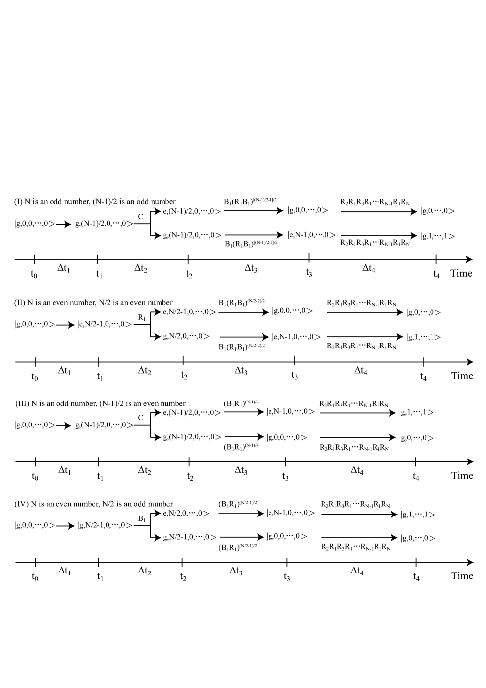
Figure 8: Schematic diagrams for preparing GHZ states of $N$ membranes: (I) both $N$ and $(N-1)/2$ are odd numbers; (II) both $N$ and $N/2$ are even numbers; (III) $N$ is an odd number and $(N-1)/2$ is an even number; (IV) $N$ is an even number and $N/2$ is an odd number.

Appendix A Preparation of W and GHZ states of $N$ membranes

Follow the method we have given in Sec. III, the W and GHZ states of $N$ membranes inside the cavity as

$$\left|\psi\right\rangle_{\mathrm{W}} = \frac{1}{\sqrt{N}}\left(\left|1,0,0,\cdots,0\right\rangle+\left|0,1,0,\cdots,0\right\rangle\right.$$ (104)

$$\left.\qquad+\cdots+\left|0,0,\cdots,0,1\right\rangle\right),$$

$$\left|\psi\right\rangle_{\mathrm{GHZ}} = \frac{1}{\sqrt{2}}\left(\left|0\right\rangle^{\otimes N}+\left|1\right\rangle^{\otimes N}\right),$$ (105)

can be generated by sequentially applying a series of red-sideband excitations, blue-sideband excitations and carrier line operations. In this appendix, we are going to give the method for generating the W and GHZ states of $N$ membranes inside the cavity under the Lamb-Dicke approximation.

Assume that the system for $N$ membranes in the cavity is prepared in the state $\left|\psi\left(t_{0}\right)\right\rangle=\left|g,0^{\otimes N}\right\rangle$ initially, then the W state of the $N$ membranes can be generated by one carrier process followed by $N$ red-sideband excitations. After the action of the carrier process for time duration $\Delta t_{1}=\pi/2\Omega$, the state of the system becomes

$$\left|\psi\left(t_{1}\right)\right\rangle=\left|e,0^{\otimes N}\right\rangle.$$ (106)

at time $t_{1}=t_{0}+\Delta t_{1}$. After that, $N$ red-sideband excitations (driving fields) are applied to the system sequentially, with frequencies $\omega_{d}=\omega_{0}-\omega_{i}$, time durations $\Delta t_{i+1}=[\arcsin\left(1/\sqrt{N+1-i}\right)]/\Omega_{1}^{i}$ and phase $\phi_{r}^{i}=\pi/2$ for $i=1,\cdots,N$. At time $t_{2}=t_{1}+\sum_{i=1}^{N}\Delta t_{i+1}$, the state of the system becomes

$$\left|\psi\left(t_{2}\right)\right\rangle = |g\rangle\otimes\frac{1}{\sqrt{N}}\left(\left|1,0,0,\cdots,0\right\rangle+\left|0,1,0,\cdots,0\right\rangle\right.$$ (107)

$$\left.\qquad+\cdots+\left|0,0,\cdots,0,1\right\rangle\right).$$

As shown in Fig. 8, we can also generate the GHZ state of $N$ membranes for the system is initially prepared in the state $\left|\psi\left(t_{0}\right)\right\rangle=\left|g,0^{\otimes N}\right\rangle$. In step (i), by sequentially applying a series of red-sideband and carrier processes, we can prepare the state

$$\left|\psi\left(t_{1}\right)\right\rangle=\left|g,\frac{N-1}{2},0^{\otimes\left(N-1\right)}\right\rangle$$ (108)

for the odd number $N$, or

$$\left|\psi\left(t_{1}\right)\right\rangle=\left|e,\left(\frac{N}{2}-1\right),0^{\otimes\left(N-1\right)}\right\rangle$$ (109)

for the even numbers $N$ and $N/2$, or

$$\left|\psi\left(t_{1}\right)\right\rangle=\left|g,\left(\frac{N}{2}-1\right),0^{\otimes\left(N-1\right)}\right\rangle$$ (110)

for the even number $N$ and odd number $N/2$.

In step (ii), if $N$ is an odd number, the system can be prepared in the state

$$\left|\psi\left(t_{2}\right)\right\rangle=\frac{1}{\sqrt{2}}\left(\left|g\right\rangle+\left|e\right\rangle\right)\otimes\left|\frac{N-1}{2},0^{\otimes\left(N-1\right)}\right\rangle,$$ (111)

by the action of the carrier process for time duration $\Delta t_{2}=\pi/4\Omega$; if both $N$ and $N/2$ are even numbers, the system can be prepared in the state

$$\left|\psi\left(t_{2}\right)\right\rangle=\frac{1}{\sqrt{2}}\left(\left|e,\frac{N}{2}-1\right\rangle+\left|g,\frac{N}{2}\right\rangle\right)\otimes\left|0^{\otimes\left(N-1\right)}\right\rangle,$$ (112)

by the red sideband excitation of the membrane one for time duration $\Delta t_{2}=\pi/4\Omega^{1}_{N/2}$, and if $N$ is an even number but $N/2$ is an odd number, the system can be prepared in the state

$$\left|\psi\left(t_{2}\right)\right\rangle=\frac{1}{\sqrt{2}}\left(\left|e,\frac{N}{2}\right\rangle+\left|g,\frac{N}{2}-1\right\rangle\right)\otimes\left|0^{\otimes\left(N-1\right)}\right\rangle,$$ (113)

by the blue sideband excitation of the membrane one for time duration $\Delta t_{2}=\pi/4\Omega^{1}_{N/2}$.

In step (iii), we can prepare the state

$$\left|\psi\left(t_{3}\right)\right\rangle=\frac{1}{\sqrt{2}}\left(\left|g,0\right\rangle+\left|e,N-1\right\rangle\right)\otimes\left|0^{\otimes\left(N-1\right)}\right\rangle$$ (114)

for all the cases in step (ii) by a series of processes as shown in Fig. 8. There are some information leaked in this step for the states $\left|g,0,0^{\otimes\left(N-1\right)}\right\rangle$ and $\left|e,N-1,0^{\otimes\left(N-1\right)}\right\rangle$ can not be prepared in synchronism, and the fidelity is shown in Fig. 9 (discussion see the Appendix B).

In step (iv), by the action of $R_{2}R_{1}R_{3}R_{1}\cdots R_{N-1}R_{1}R_{N}$ for time duration $\Delta t_{4}=\sum_{i=2}^{N-1}\pi/2\Omega^{1}_{i}+\sum_{i=2}^{N}\pi/2\Omega^{i}_{1}$, we get the state

$$\left|\psi\left(t_{4}\right)\right\rangle=\left|g\right\rangle\otimes\frac{1}{\sqrt{2}}\left(\left|0^{\otimes N}\right\rangle+\left|1^{\otimes N}\right\rangle\right).$$ (115)

Thus we have prepared $N$ membranes in the GHZ state and the optical field in the cavity in the ground state $\left|g\right\rangle$.

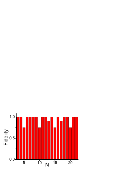
Figure 9: Fidelity for preparing GHZ state $\frac{1}{\sqrt{2}}\left(\left|0^{\otimes N}\right\rangle+\left|1^{\otimes N}\right\rangle\right)$ from $N=3$ to $N=22$.

Appendix B The information leakage caused by non-synchronization

In the preparation of the NOON state and GHZ state in the Lamb-Dicke regime, we need the processes for preparation two different states synchronically. For example, in the preparation of state $\left(\left|2,0\right\rangle+\left|0,2\right\rangle\right)/\sqrt{2}$, the transitions $\left|g,1,1\right\rangle\rightarrow\left|e,1,0\right\rangle$, and $\left|e,0,1\right\rangle\rightarrow\left|g,0,2\right\rangle$ should be synchronized. In the other words, the time duration should satisfy Eq. (56). However, we find that Eq. (56) can only be satisfied in the infinite approximation. In this appendix, we will discuss the information leakage caused by this type of non-synchronization.

Without lose of generality, suppose that the state of the system at time $t$ is given as

$$\left|\psi\left(t\right)\right\rangle=\frac{1}{\sqrt{2}}\left|e,n-1,n^{\prime}\right\rangle+\frac{1}{\sqrt{2}}\left|g,m,m^{\prime}\right\rangle$$ (116)

and at the following time $t^{\prime}$, we need to prepare the state

$$\left|\psi\left(t^{\prime}\right)\right\rangle=\frac{1}{\sqrt{2}}\left|g,n,n^{\prime}\right\rangle+\frac{1}{\sqrt{2}}\left|e,m-1,m^{\prime}\right\rangle.$$ (117)

So we drive the optical cavity with a laser field resonant to the first red sideband of the first membrane for time duration $\Delta t=t^{\prime}-t$, and the system evolves into

$$\left|\psi\left(t^{\prime}\right)\right\rangle = \frac{1}{\sqrt{2}}[\cos\left(\Omega_{n}^{1}\Delta t\right)\left|e,n-1,n^{\prime}\right\rangle$$ (118)

$$-ie^{i\phi_{r}^{1}}\sin\left(\Omega_{n}^{1}\Delta t\right)\left|g,n,n^{\prime}\right\rangle$$

$$+\cos\left(\Omega_{m}^{1}\Delta t\right)\left|g,m,m^{\prime}\right\rangle$$

$$-ie^{-i\phi_{r}^{1}}\sin\left(\Omega_{m}^{1}\Delta t\right)\left|e,m-1,m^{\prime}\right\rangle].$$

where $\Omega_{n}^{1}=\Omega\eta_{1}\sqrt{n}$, $\Omega_{m}^{1}=\Omega\eta_{1}\sqrt{m}$.

In order to make sure that the system at the time $t^{\prime}$ is in the state given by Eq.(117), the time duration $\Delta t$ should satisfy the equations

$$\sin\left(\Omega_{n}^{1}\Delta t\right)=\pm 1,\sin\left(\Omega_{m}^{1}\Delta t\right)=\pm 1.$$ (119)

Eq.(119) can be equal to the equations

$$(\Omega_{n}^{1}\pm\Omega_{m}^{1})\Delta t=p\pi,\Omega_{m}^{1}\Delta t=(q+\frac{1}{2})\pi,$$ (120)

where $p$ and $q$ are positive integral numbers. Taking $\Omega_{n}^{1}/\Omega_{m}^{1}=\sqrt{n/m}$ (suppose $n\geq m$), Eq.(120) can be rewritten as

$$\left(\sqrt{\frac{n}{m}}\pm 1\right)\left(q+\frac{1}{2}\right)=p.$$ (121)

for choosing appreciate integral numbers $p$ and $q$.

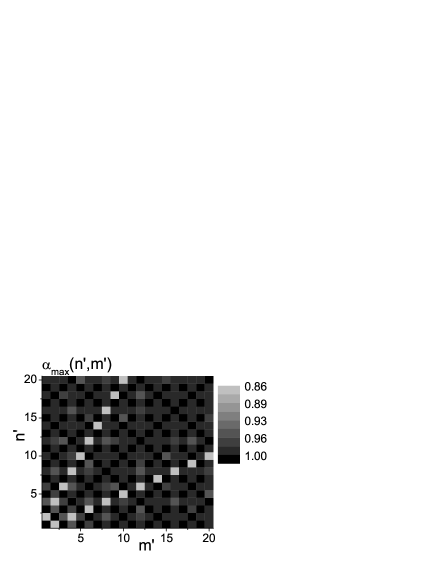
Figure 10: The maximal value of $\alpha$ versus $n^{\prime}$ and $m^{\prime}$.

According to the rate of the two angular frequencies, the solutions can be divided into three cases:

(i) If $\sqrt{n/m}$ is a rational number, we can rewrite it as a quotient of integers,

$$\sqrt{\frac{n}{m}}=\frac{n^{\prime}}{m^{\prime}},$$ (122)

where $n^{\prime}$ and $m^{\prime}$ are integers and they have no common factors. Substitute Eq.(122) into Eq.(121), we get

$$\left(\frac{n^{\prime}\pm m^{\prime}}{m^{\prime}}\right)\left(\frac{2q+1}{2}\right)=p.$$ (123)

If both $n^{\prime}$ and $m^{\prime}$ are odd, then there are integral numbers $p$ and $q$ that satisfy Eq.(123) exactly.

(ii) If $\sqrt{n/m}=n^{\prime}/m^{\prime}$ is a rational number, and one of them ($n^{\prime}$ and $m^{\prime}$) is even, there are no integral numbers satisfying Eq.(123). However, there are integral numbers can satisfy the following equations for appreciate value of $\Delta t$,

$$\sin\left(\Omega_{n}^{1}\Delta t\right)=\pm\sin\left(\Omega_{m}^{1}\Delta t\right)=\pm\alpha,$$ (124)

where $\alpha$ is given by

$$\alpha=\left|\sin\left(\frac{m^{\prime}}{n^{\prime}\pm m^{\prime}}p\pi\right)\right|.$$ (125)

By the increase of $p$, $\alpha$ oscillates periodically with a period $n^{\prime}\pm m^{\prime}$. The maximal value of $\alpha$ as function of $n^{\prime}$ and $m^{\prime}$ (denoted by $\alpha_{max}(n^{\prime},m^{\prime})$) is shown in Fig.10. From the figure we can see that $\alpha_{max}(n^{\prime},m^{\prime})\geq 0.86$, and $\alpha_{max}(n^{\prime},m^{\prime})=1$ for the case that both $n^{\prime}$ and $m^{\prime}$ are odd, which is agree with the result given above.

(iii) If $\sqrt{n/m}$ is an irrational number, there are no integral numbers ($p$ and $q$) that satisfy Eq.(121) exactly, but there is a rational number $n^{\prime}/m^{\prime}$ (both $n^{\prime}$ and $m^{\prime}$ are odd) that can be infinitely close to $\sqrt{n/m}$. So we can get appreciate value of $\Delta t$ which can satisfy Eq.(121) in the infinite approximation.

References

- (1) M. A. Nielsen and I. L. Chuang, Quantum Computation and Quantum Information (Cambridge University Press, Cambridge, 2000).
- (2) J. M. Raimond, M. Brune, and S. Haroche, Rev. Mod. Phys. 73, 565 (2001).
- (3) P. G. Kwiat, K. Mattle, H. Weinfurter, A. Zeilinger, A. V. Sergienko, and Y. Shih. Phys. Rev. Lett. 75, 4337 (1995).
- (4) E. Hagley, X. Maître, G. Nogues, C. Wunderlich, M. Brune, J. M. Raimond, and S. Haroche, Phys. Rev. Lett. 79, 1 (1997).
- (5) C. Sackett, D. Kielpinsky, B. King, C. Langer, V. Meyer, C. Myatt, M. Rowe, Q. Turchette, W. Itano, D. Wineland, and C. Monroe, Nature (London) 404, 256 (2000)
- (6) M. Neeley, R. C. Bialczak, M. Lenander, E. Lucero, M. Mariantoni, A. D. O Connell, D. Sank, H. Wang, M. Weides, J. Wenner, Y. Yin, T. Yamamoto, A. N. Cleland, and J. M. Martinis, Nature (London) 467, 570 (2010).
- (7) L. DiCarlo, M. D. Reed, L. Sun, B. R. Johnson, J. M. Chow, J. M. Gambetta, L. Frunzio, S. M. Girvin, M. H. Devoret, and R. J. Schoelkopf, Nature (London) 467, 574 (2010).
- (8) D. J. Wineland and D. Leibfried, Laser Phys. Lett. 8, 175 (2011).
- (9) M. Poot and H.S.J. van der Zant, Phys. Rep. 511, 273 (2012).
- (10) D. Leibfried, R. Blatt, C. Monroe, and D. Wineland, Rev. Mod. Phys. 75, 281 (2003).
- (11) H. Moya-Cessa, F. Soto-Eguibar, J. M. Vargas-Martínez, R. Juárez-Amaro, and A. Zún̋iga-Segundo, Phys. Rep. 513, 229 (2012).
- (12) S. B. Zheng, Phys. Rev. A 63, 015801 (2000); X. B. Zou, K. Pahlke, and W. Mathis, Phys. Rev. A 65, 045801 (2002).
- (13) L. F. Wei, Y. X. Liu, and F. Nori, Phys. Rev. A 70, 063801 (2004).
- (14) Y. X. Liu, L. F. Wei, and F. Nori, Europhys. Lett. 67, 941 (2004).
- (15) A. D. O Connell, M. Hofheinz, M. Ansmann, R. C. Bialczak, M. Lenander, E. Lucero, M. Neeley, D. Sank, H. Wang, M. Weides, J. Wenner, J. M. Martinis, and A. N. Cleland, Nature (London) 464, 697 (2010).
- (16) F. Xue, Y. X. Liu, C. P. Sun, and F. Nori, Phys. Rev. B 76, 064305 (2007).
- (17) S. Gigan, H. R. Böhm, M. Paternostro, F. Blaser, G. Langer, J. B. Hertzberg, K. C. Schwab, D. Bäuerle, M. Aspelmeyer, and A. Zeilinger, Nature (London) 444, 67 (2006).
- (18) O. Arcizet, P. F. Cohadon, T. Briant, M. Pinard, and A. Heidmann, Nature (London) 444, 71 (2006).
- (19) A. Schliesser, P. Del’Haye, N. Nooshi, K. J. Vahala, and T. J. Kippenberg, Phys. Rev. Lett. 97, 243905 (2006).
- (20) I. Wilson-Rae, N. Nooshi, W. Zwerger, and T. J. Kippenberg, Phys. Rev. Lett. 99, 093901 (2007).
- (21) F. Marquardt, J. P. Chen, A. A. Clerk, and S. M. Girvin, Phys. Rev. Lett. 99, 093902 (2007).
- (22) J. D. Teufel, J. W. Harlow, C. A. Regal, and K. W. Lehnert, Phys. Rev. Lett. 101, 197203 (2008).
- (23) J. D. Thompson, B. M. Zwickl, A. M. Jayich, F. Marquardt, S. M. Girvin, and J. G. E. Harris, Nature (London) 452, 72 (2008).
- (24) A. Schliesser, R. Rivière, G. Anetsberger, O. Arcizet, and T. J. Kippenberg, Nature Phys. 4, 415 (2008).
- (25) S. Gröblacher, J. B. Hertzberg, M. R. Vanner, G. D. Cole, S. Gigan, K. C. Schwab, and M. Aspelmeyer, Nature Phys. 5, 485 (2009).
- (26) T. Rocheleau, T. Ndukum, C. Macklin, J. B. Hertzberg, A. A. Clerk, and K. C. Schwab, Nature (London) 463, 72 (2010).
- (27) Y. S. Park and H. Wang, Nature Phys. 5, 489 (2009).
- (28) A. Schliesser, O. Arcizet, R. Rivière, G. Anetsberger, and T. J. Kippenberg, Nature Phys. 5, 509 (2009).
- (29) J. D. Teufel, T. Donner, D. Li, J. W. Harlow, M. S. Allman, K. Cicak, A. J. Sirois, J. D. Whittaker, K. W. Lehnert, and R. W. Simmonds, Nature (London) 475, 359 (2011).
- (30) J. Chan, T. P. M. Alegre, A. H. Safavi-Naeini, J. T. Hill, A. Krause, S. Gröblacher, M. Aspelmeyer, and O. Painter, Nature (London) 478, 89 (2011).
- (31) E. Verhagen, S. Deléglise, S. Weis, A. Schliesser, and T. J. Kippenberg, Nature (London) 482, 63 (2012).
- (32) J. Q. Liao and C. K. Law, Phys. Rev. A 84, 053838 (2011).
- (33) T. J. Kippenberg and K. J. Vahala, Science 321, 1172 (2008).
- (34) F. Marquardt and S. M. Girvin, Physics 2, 40 (2009).
- (35) C. Genes, A. Mari, D. Vitali, P. Tombesi, Adv. At. Mol. Opt. Phys. 57, 33 (2009).
- (36) D. Vitali, S. Gigan, A. Ferreira, H. R. Böhm, P. Tombesi, A. Guerreiro, V. Vedral, A. Zeilinger, and M. Aspelmeyer, Phys. Rev. Lett. 98, 030405 (2007).
- (37) D. Vitali, P. Tombesi, M. J. Woolley, A. C. Doherty, and G. J. Milburn, Phys. Rev. A 76, 042336 (2007).
- (38) A. Mari and J. Eisert, Phys. Rev. Lett. 103, 213603 (2009).
- (39) H. X. Miao, S. Danilishin, and Y. B. Chen, Phys. Rev. A 81, 052307 (2012).
- (40) L. Tian and S. M. Carr, Phys. Rev. B 74, 125314 (2006).
- (41) S. G. Hofer, W. Wieczorek, M. Aspelmeyer, and K. Hammerer, Phys. Rev. A 84, 052327 (2011).
- (42) S. Barzanjeh, M. Abdi, G. J. Milburn, P. Tombesi, and D. Vitali, Phys. Rev. Lett. 109, 130503 (2012).
- (43) Y. D. Wang and A. A. Clerk, Phys. Rev. Lett. 108, 153603 (2012).
- (44) L. Tian, Phys. Rev. Lett. 108, 153604 (2012).
- (45) M. Paternostro, D. Vitali, S. Gigan, M. S. Kim, C. Brukner, J. Eisert, and M. Aspelmeyer, Phys. Rev. Lett. 99, 250401 (2007).
- (46) C. Genes, D. Vitali and P. Tombesi, New J. Phys. 10, 095009 (2008).
- (47) C. Genes, A. Mari, P. Tombesi, and D. Vitali, Phys. Rev. A 78, 032316 (2008).
- (48) A. Xuereb, M. Barbieri, and M. Paternostro, Phys. Rev. A 86, 013809 (2012).
- (49) M. Abdi, A. R. Bahrampour, and D. Vitali, Phys. Rev. A 86, 043803 (2012).
- (50) C. Genes, D. Vitali, and P. Tombesi, Phys. Rev. A 77, 050307 (2008).
- (51) H. Ian, Z. R. Gong, Y. X. Liu, C. P. Sun, and F. Nori, Phys. Rev. A 78, 013824 (2008).
- (52) K. Hammerer, M. Aspelmeyer, E. S. Polzik, and P. Zoller, Phys. Rev. Lett. 102, 020501 (2009).
- (53) L. Zhou, Y. Han, J. T. Jing, and W. P. Zhang, Phys. Rev. A 83, 052117 (2011).
- (54) G. De Chiara, M. Paternostro, and G. M. Palma, Phys. Rev. A 83, 052324 (2011).
- (55) C. Genes, H. Ritsch, M. Drewsen, and A. Dantan, Phys. Rev. A 84, 051801 (2011).
- (56) L. H. Sun, G. X. Li, and Z. Ficek, Phys. Rev. A 85, 022327 (2012).
- (57) B. Rogers, M. Paternostro, G. M. Palma, and G. De Chiara, Phys. Rev. A 86, 042323 (2012).
- (58) H. Jing, X. Zhao, and L. F. Buchmann Phys. Rev. A 86, 065801 (2012).
- (59) Y. Chang and C. P. Sun, Phys. Rev. A 83, 053834 (2011).
- (60) M. Wallquist, K. Hammerer, P. Zoller, C. Genes, M. Ludwig, F. Marquardt, P. Treutlein, J. Ye, and H. J. Kimble, Phys. Rev. A 81, 023816 (2010).
- (61) Sh. Barzanjeh, M. H. Naderi, and M. Soltanolkotabi, Phys. Rev. A 84, 063850 (2011).
- (62) S. Mancini, V. Giovannetti, D. Vitali and P. Tombesi, Phys. Rev. Lett. 88, 120401 (2002).
- (63) S. Pirandola, D. Vitali, P. Tombesi, and S. Lloyd, Phys. Rev. Lett. 97, 150403 (2006).
- (64) M. J. Hartmann and M. B. Plenio, Phys. Rev. Lett. 101, 200503 (2008).
- (65) M. Ludwig, K. Hammerer, and F. Marquardt, Phys. Rev. A 82, 012333 (2010).
- (66) M. Bhattacharya, P. L. Giscard, and P. Meystre, Phys. Rev. A 77, 030303 (2008).
- (67) M. Schmidt, M. Ludwig and F. Marquardt, New J. Phys. 14, 125005 (2012).
- (68) G. Vacanti, M. Paternostro, G. M. Palma, and V. Vedral, New J. Phys. 10, 095014 (2008).
- (69) K. Borkje, A. Nunnenkamp, and S. M. Girvin, Phys. Rev. Lett. 107, 123601 (2011).
- (70) L. Mazzola, and M. Paternostro, Phys. Rev. A 83, 062335 (2011).
- (71) C. Joshi, J. Larson, M. Jonson, E. Andersson, and P. Ohberg, Phys. Rev. A 85, 033805 (2012).
- (72) M. Abdi, S. Pirandola, P. Tombesi, and D. Vitali, Phys. Rev. Lett. 109, 143601 (2012).
- (73) B. Pepper, R. Ghobadi, E. Jeffrey, C. Simon, and D. Bouwmeester, Phys. Rev. Lett. 109, 023601 (2012).
- (74) M. R. Vanner, M. Aspelmeyer, M. S. Kim, Phys. Rev. Lett. 110, 010504 (2013).
- (75) X. W. Xu, H. Wang, J. Zhang, and Yu-xi Liu, arXiv:1210.0070.
- (76) M. Bhattacharya, H. Uys, and P. Meystre, Phys. Rev. A 77, 033819 (2008).
- (77) M. Bhattacharya and P. Meystre, Phys. Rev. A 78, 041801(R) (2008).
- (78) A. Tomadin, S. Diehl, M. D. Lukin, P. Rabl, and P. Zoller, Phys. Rev. A 86, 033821 (2012).
- (79) J. Q. Liao, H. K. Cheung, and C. K. Law Phys. Rev. A 85, 025803 (2012).
- (80) A. Xuereb, C. Genes, and A. Dantan, Phys. Rev. Lett. 109, 223601 (2012).
- (81) M. Schmidt, M. Ludwig, and F. Marquardt, New J. Phys. 14, 125005 (2012).
- (82) C. A. Holmes, C. P. Meaney, and G. J. Milburn, Phys. Rev. E 85, 066203 (2012).
- (83) H. Seok, L. F. Buchmann, S. Singh, and P. Meystre, Phys. Rev. A 86, 063829 (2012).
- (84) F. Massel, S. U. Cho, J. M. Pirkkalainen, P. J. Hakonen, T. T. Heikkilä, and M. A. Sillanpää, Nature Communications 3, 987 (2012).
- (85) M. Born and E. Wolf, Principles of optics: electromagnetic theory of propagation, interference and diffraction of light (Cambridge University Press, Cambridge, 1999).
- (86) A. Xuereb, P. Domokos, J. Asbóth, P. Horak, and T. Freegarde, Phys. Rev. A 79, 053810 (2009).
- (87) A. Xuereb, T. Freegarde, P. Horak, P. Domokos, Phys. Rev. Lett. 105, 013602 (2010).
- (88) S. A. R. Horsley, M. Artoni, and G. C. La Rocca, Phys. Rev. A 86, 053820 (2012).
- (89) M. B. Spencer and W. E. Lamb, Phys. Rev. A 5, 893 (1972).
- (90) W. J. Fader, IEEE J. Quantum Electron. 21, 1838 (1985).
- (91) C. K. Law, Phys. Rev. A 51, 2537 (1995).
- (92) J. J. Bollinger, W. M. Itano, D. J. Wineland, and D. J. Heinzen, Phys. Rev. A 54, R4649 (1996).
- (93) W. Dür, G. Vidal, and J. I. Cirac, Phys. Rev. A 62, 062314 (2000).
- (94) K. W. Murch, K. L. Moore, S. Gupta, and D. M. Stamper- Kurn, Nat. Phys. 4, 561 (2008).
- (95) F. Brennecke, S. Ritter, T. Donner, and T. Esslinger, Science 322, 235 (2008).
- (96) D. E. Chang, C. A. Regal, S. B. Papp, D. J. Wilson, J. Ye, O. Painter, H. J. Kimble and P. Zoller, Proc. Natl. Acad. Sci. USA 107, 1005 (2010).
- (97) O. Romero-Isart, M. L. Juan, R. Quidant and J. I. Cirac, New J. Phys. 12, 033015 (2010).
- (98) O. Romero-Isart, A. C. Pflanzer, M. L. Juan, R. Quidant, N. Kiesel, M. Aspelmeyer and J. I. Cirac, Phys. Rev. A 83, 013803 (2011).
- (99) T. C. Li, S. Kheifets, and M. G. Raizen, Nature Physics 7, 527 (2011).
- (100) M. Eichenfield, J. Chan, R. M. Camacho, K. J. Vahala, and O. Painter, Optomechanical crystals, Nature 462, 78 (2009)