Analytical treatment of long-term observations of the day-night asymmetry for solar neutrinos

Abstract

The Earth’s density distribution can be approximately considered piecewise continuous at the scale of two-flavor oscillations of typical solar neutrinos, such as the beryllium-7 and boron-8 neutrinos. This quite general assumption appears to be enough to analytically calculate the day-night asymmetry factor for such neutrinos. Using the explicit time averaging procedure, we show that, within the leading-order approximation, this factor is determined by the electron density within about one oscillation length under the detector, namely, in the Earth’s crust (and upper mantle for high-energy neutrinos). We also evaluate the effect of the inner Earth’s structure on the observed asymmetry and show that it is suppressed and mainly comes from the neutrinos observed near the winter and summer solstices. As a result, we arrive at the strict interval constraint on the asymmetry, which is valid within quite a wide class of Earth models.

I Introduction

The effect of neutrino oscillations in vacuum lies beyond the Standard Model and is thus interesting both from the theoretical and experimental points of view. The oscillations in medium have also been studied since Wolfenstein, who showed that neutrinos acquire a specific flavor-dependent potential due to coherent forward scattering on the matter Wolfenstein . As a result, the neutrino propagation in medium should demonstrate the conversion from one flavor into another (i.e. flavor oscillations), even if the vacuum mixing is negligible. This spectacular result is known as the Mikheev–Smirnov–Wolfenstein effect MikheevSmirnov and suffices to explain the deficit of observed solar electron neutrinos Bethe . According to Mikheev and Smirnov, the leading-order estimation for the electron neutrino flux depends only on the points where the neutrino was born (the core of the Sun) and absorbed (the detector). However, the properties of the medium between these two points can also slightly affect the flavor composition of the observed neutrino flux, leading, in particular, to the day-night (solar neutrino flavor) asymmetry Carlson ; Baltz . The latter effect being crucial for the entire flavor oscillations framework, a number of experiments were set up to catch this slight flavor composition variation resulting from the nighttime neutrino propagation through the Earth SNO_DNA ; SuperK_DNA ; Borexino . Some experiments, which should be sensitive enough to distinguish the effect, are also planned in the next decade and are now under construction LENA .

However, one should hold in mind that, in order to make a conclusion on the expected presence of the day-night asymmetry, one needs not only the experimental data (in terms of event rates and energy spectra) but also a convenient theoretical prediction. First experiments in neutrino oscillations were only aimed at outlining the domains in the neutrino mass and mixing parameter space which do not contradict the observed rates. For such needs, the theoretical estimations obtained using numerical simulations are quite acceptable (see, e.g., BahcallKrastev ). Indeed, although numerical experiments can lack perfect accuracy in some regimes and do not give general results, the calculation of the desired effect can be performed for the entire parameter space without drastic algorithm changes. Therefore, using numerical predictions, one could more or less interpret the experimental data in terms of domains in this parameter space which are excluded. But now that various neutrino experiments have yielded a considerable amount of data on the vacuum neutrino mixing SNO ; KamLand ; Borexino1 and its parameters are fixed quite firmly, the question is whether other neutrino oscillation effects to be observed are consistent with the framework accepted so far. Namely, one may ask: how should one compare the present and future experimental data on the day-night asymmetry with the theory of neutrino oscillations in order to make an ultimate conclusion about their agreement within the allowed class of Earth and solar models? The latter issue requires a formalism able to give strict constraints (in a form of an interval with fixed boundaries) on the predicted asymmetry within certain approximations, but valid within quite a wide class of the Earth and solar models. Developing such a formalism constitutes the principal goal of the present paper. In particular, using it, we readily find the constraints on the day-night asymmetry for beryllium and boron neutrinos observed in such experiments as SNO, Super-Kamiokande, and Borexino SNO_DNA ; SuperK_DNA ; Borexino .

Within the neutrino oscillations framework, it is common to use the Schroedinger-like equation to describe the spatial variations of the neutrino flavor Wolfenstein ; MikheevSmirnov . Within the two-flavor approximation, the Schroedinger problem is posed in terms of the $2\times 2$ flavor evolution matrix (operator) $R(x,x_{0})$, whose elements are the neutrino flavor transition amplitudes after traveling from point $x_{0}$ to $x$. The evolution equation and the initial condition read, respectively,

$$\frac{\partial R(x,x_{0})}{\partial x} = -\mathrm{i}\lambda A(x)R(x,x_{0}),$$ (1)

$$R(x_{0},x_{0}) = \mathds{1},$$ (2)

where the matrix Hamiltonian is a point-dependent linear combination of the Pauli matrices,

$$A(x)=a(x)\sigma_{3}+b\sigma_{1},$$ (3)

$$a(x)=-\cos 2\theta_{0}+\frac{2EV(x)}{{\scriptstyle\Delta}m^{2}},\qquad b=\sin 2\theta_{0}.$$ (4)

Here, $\theta_{0}$ is the vacuum mixing angle, $E$ is the neutrino energy, ${\scriptstyle\Delta}m^{2}$ is the difference between neutrino masses squared, and $V(x)=\sqrt{2}G_{\text{F}}N_{e}(x)$ is the Wolfenstein potential, which is proportional to the electron density in the medium $N_{e}$ and the Fermi constant $G_{\text{F}}=1.17\times 10^{-11}\text{ MeV}^{-2}$. The constant coefficient $\lambda={\scriptstyle\Delta}m^{2}/4E$ is the reciprocal vacuum neutrino oscillation length, up to the factor of $\pi$,

$$\ell_{\mathrm{osc}}=\frac{4\pi E}{{\scriptstyle\Delta}m^{2}}=\frac{\pi}{\lambda}.$$ (5)

Equation (1) defines a one-parametric subgroup of $SU(2)$ and hence of $SO(3)$, the translation along $x$ being the group operation. In this sense, equation (1) is analogous to the Bargmann–Michel–Telegdi equation b1 in the spinor representation b4 . It is well known that the solution of the matrix linear ordinary differential equation, such as (1), can be represented as a time-ordered exponential (Dyson expansion) DiffEquations . However, in the case of general $N_{e}(x)$ profile, the solution in terms of an analytical function of the matrix argument (i.e., without a symbolic operation such as time ordering) appears to be too challenging to find. In the recent investigations, considerable progress was made in finding exact solutions of Eq. (1) in certain special cases b5 ; b11 ; nevertheless, the general approach to this kind of equation still remains to be approximate.

It was first naturally accepted that numerical simulations could give exhaustive results here and, in a sense, resolve the analytical difficulties that arise in the context of such equations. For instance, a numerical approach was employed in BahcallKrastev ; Lisi to find the domains in the neutrino mixing parameter space where the day-night asymmetry should be potentially observable. However, as mentioned above, estimations obtained with numerical techniques are not always reliable enough. In particular, in the large-${\scriptstyle\Delta}m^{2}$ regime, which has now proved to be realistic SNO ; KamLand , the oscillation length (5) becomes small, and numerical evaluation of rapidly oscillating solutions introduces large uncertainties. The numerical time averaging of the flavor observation rates also becomes inaccurate in this regime. This effect is especially strong for low-energy neutrinos, including beryllium neutrinos; probably, due to this fact, the large-${\scriptstyle\Delta}m^{2}$ and low-energy area was not covered by original numerical simulations BahcallKrastev . Therefore, obtaining stringent constraints on the day-night asymmetry factor for the continuous measurement of small-length neutrino oscillations favors the analytical approach.

Quite a large number of publications are devoted to the analysis of such approximate analytical solutions. Probably the most effective technique for finding the approximate solutions of matrix linear differential equations, such as (1), is the so-called Magnus expansion Magnus , which is a generalization of the Baker–Campbell–Hausdorff formula Campbell . This approach provides the solution up to any order of approximation, as well as the constraints on the remainder terms MagnusApps . Unfortunately, this technique Olivo90 ; Olivo ; Olivo08 ; IoannisianSmirnov09 , as well as other general methods (see, e.g., Ohlsson ; Akhmedov08 ), does not readily provide a way to find the solution in its explicit and practically usable form, not firmly fixing the Earth model, namely, $N_{e}(x)$ density distribution. It is thus desirable to find an approximate analytical solution of equation (1), which is valid under quite general assumptions about the electron density profile $N_{e}(x)$. This idea was developed in Wei ; IoannisianSmirnov04 ; AkhmedovValle .

As it was mentioned earlier in this section, in our paper, we are not only aiming at finding the relevant approximate expressions, but also at analyzing their accuracy and applicability domain. Namely, in section II, we find the approximate solutions for the flavor evolution matrix inside the Earth, and then, in section III, we arrive at the observation probabilities for the neutrinos of different flavors. These probabilities are finally subjected to the averaging procedure due to the continuous observation of the solar neutrinos throughout the year (Sec. III.2), and the results of this averaging are discussed in section IV. The magnitude of the day-night asymmetry appears to be sensitive to the non-trivial structure of the Earth’s crust under the neutrino detector, so the effect of the crust is paid special attention in section III.3. The uncertainties of our estimation are also discussed in section IV, in the interesting cases of beryllium and boron neutrinos. We analyze the sources of such uncertainties and finally compare our results with the numerical simulation. The detailed derivation of the approximate solutions for the evolution operator is moved to the Appendix to make the flow of the paper less complicated.

II The Density Profile and the Evolution Matrix

In our investigation, we use the model electron density profile $N_{e}(x)$ with $n-1$ narrow segments, where it changes steeply, separated by $n$ wide though sloping segments. Let us call these segments cliffs and valleys, respectively. Let the cliffs be localized near points $x_{j}$, $j=\overline{1,n-1}$, namely, occupy segments $[x_{j}^{-},x_{j}^{+}]$ of widths $\epsilon_{j}$, where $x_{j}^{\pm}\equiv x_{j}\pm\epsilon_{j}/2$. Then the valleys are $[x_{j-1}^{+},x_{j}^{-}]$ and have the widths $L_{j}\approx x_{j}-x_{j-1}$. In fact, this kind of model is a good approximation for the Earth’s density profile known in geophysics, where it corresponds to the so-called Preliminary Reference Earth Model (PREM)  Anderson ; Anderson1 . In the present section, we will assume that the above segments can be chosen in such a way that the inequality

$$\epsilon_{j}\ll\ell_{\text{osc}}\ll L_{j}$$ (6)

takes place, i.e. the cliffs are narrow and the valleys are wide compared with the oscillation length. In the following, we will briefly call such density distribution piecewise continuous.

Let us note in advance (see Sec. IV for details) that for the energies of beryllium neutrinos ($E=0.862\text{MeV}$, $\ell_{\text{osc}}\approx 30~{}\text{km}$) and, to some extent, boron neutrinos ($E\sim 5-10~{}\text{MeV}$, $\ell_{\text{osc}}\approx 150-300~{}\text{km}$), the Earth’s layers can be divided into cliffs and valleys satisfying (6), as well as into a number of layers whose widths are of the order of the oscillation length, while the density variations are small. One can show that the contributions of the latter segments can be easily considered in a manner very similar to those of the cliffs, hence we do not consider them until Sec. III.3 where they will be paid special attention. In the present section, it is enough to note that the valley-cliff classification depends on the neutrino energy. It is also worth saying here that during the night, the neutrino ray traverses different paths through the Earth, thus, the lengths $\epsilon_{j}$ and $L_{j}$ vary. However, assumption (6) holds for the most part of the night.

The total flavor evolution operator for our piecewise continuous density profile equals the matrix product of the evolution operators for all cliffs and valleys. Within each of these segments, the two small parameters arise: the first of them,

$$\eta=\frac{2EV(x)}{{\scriptstyle\Delta}m^{2}}\lesssim\begin{cases}1.0\times 10^{-2},&\qquad E=0.862~{}\text{MeV},\\ 1.2\times 10^{-1},&\qquad E\sim 10~{}\text{MeV},\end{cases}$$ (7)

due to the relatively small density of the Earth IoannisianSmirnov04 ; IoannisianSmirnov05 , while the second parameter due to the piecewise continuous structure of the density profile,

$$\delta=\left\{\begin{array}[]{ll}\ell_{\text{osc}}/L_{j}&\text{for $j$th valley,}\\ \epsilon_{j}/\ell_{\text{osc}}&\text{for $j$th cliff.}\end{array}\right.$$ (8)

The smallness of parameter $\delta$ will be discussed in Sec. IV.

The evolution matrix for each segment, as well as the total evolution matrix, can be subjected to the following unitary transformations Olivo08 :

$$R(x,x_{0}) = Z^{+}(x)Y(\psi(x))R_{0}(x,x_{0})Y^{-1}(\psi(x_{0}))Z^{-}(x_{0}),$$ (9)

$$Z^{\pm}(x) = \frac{1}{\sqrt{2}}\left\{\sqrt{1-\frac{a(x)}{\omega(x)}}\pm\mathrm{i}\sigma_{2}\sqrt{1+\frac{a(x)}{\omega(x)}}\,\right\},$$ (10)

$$Y(\psi(x)) = \cos\psi(x)+\mathrm{i}\sigma_{3}\sin\psi(x)=\exp\{\mathrm{i}\sigma_{3}\psi(x)\},$$ (11)

where $\omega(x)=\sqrt{a^{2}(x)+b^{2}}$ and $\psi(x)=\lambda\int\omega(x)\mathrm{d}{x}$ is the corresponding phase incursion. For the calculations which follow, it is also useful to introduce the effective mixing angle in the medium $\theta(x)\in[0,\pi/2]$  MikheevSmirnov , which is defined by the expressions

$$\cos 2\theta(x)=-\frac{a(x)}{\omega(x)},\qquad\sin 2\theta(x)=\frac{b}{\omega(x)}.$$ (12)

In terms of this angle,

$$Z^{\pm}(x)=\exp\{\pm\mathrm{i}\sigma_{2}\theta(x)\}.$$ (13)

The transformation with matrices $Z^{\pm}(x)$ locally diagonalizes the Hamiltonian $H(x)$ in the point $x$. It thus makes the complete diagonalization in the homogeneous case $N_{e}(x)=\mathrm{const}$ MikheevSmirnov . The transformation with the operator $Y(\psi(x))$ isolates the effect of the medium inhomogeneity, the transformed evolution matrix $R_{0}(x,x_{0})$ satisfying the equation

$$\frac{\partial R_{0}(x,x_{0})}{\partial x}=-\mathrm{i}\dot{\theta}(x)\sigma_{2}e^{2\mathrm{i}\sigma_{3}\psi(x)}R_{0}(x,x_{0}),$$ (14)

where the dot over $\theta$ denotes the gradient

$$\dot{\theta}(x)\equiv\partial_{x}\theta(x)=\frac{b\,\partial_{x}{a}(x)}{2\omega^{2}(x)}.$$ (15)

Due to the fact that the neutrino detector is homogeneous ($\dot{\theta}(x)=0$), Eq. (14) has a well-defined and physically relevant $x\to+\infty$ limit for any fixed $x_{0}$. Moreover, asymptotically convergent behavior of such systems of differential equations is stated by the Levinson’s theorem DiffEquations .

In the homogeneous case, the equation above is trivial, $R_{0}(x,x_{0})\equiv\mathds{1}$. However, in the valley $[x_{j}^{+},x_{j+1}^{-}]$, the slow change of the density $N_{e}(x)$ enables us to use the so-called adiabatic approximation leading to the same result MikheevSmirnov

$$R_{0}(x_{j+1}^{-},x_{j}^{+})=\mathds{1}+\mathit{O}({\scriptstyle\Delta}\eta\ \delta_{\text{valley}}),$$ (16)

where the remainder term is a (generally speaking, non-diagonal) matrix and ${\scriptstyle\Delta}\eta$ is the variation of the density parameter $\eta$ over the valley. On the other hand, if the Wolfenstein potential undergoes a considerable change within the narrow cliff $[x_{j}^{-},x_{j}^{+}]$ with the phase incursion ${\scriptstyle\Delta}\psi\ll 2\pi$, then we get

$$R_{0}(x_{j}^{+},x_{j}^{-})=\exp\left\{-\mathrm{i}\sigma_{2}{\scriptstyle\Delta}\theta_{j}e^{2\mathrm{i}\sigma_{3}\psi(x_{j}^{-})}\right\}+\mathit{O}(\eta\delta_{\text{cliff}}),$$ (17)

where ${\scriptstyle\Delta}\theta_{j}\equiv\theta(x_{j}^{+})-\theta(x_{j}^{-})=\mathit{O}(\eta)$ is the jump of the effective mixing angle on the $j$th cliff. Moreover, one can show that within the more accurate $O(\eta\delta)$ approximation, the above expressions take the form (see the Appendix)

$$R_{0}(x_{j+1}^{-},x_{j}^{+}) = \exp\left\{-\frac{\mathrm{i}\sigma_{1}}{2\lambda}\left[e^{2\mathrm{i}\sigma_{3}\psi(x_{j+1}^{-})}\dot{\theta}(x_{j+1}^{-})-e^{2\mathrm{i}\sigma_{3}\psi(x_{j}^{+})}\dot{\theta}(x_{j}^{+})\right]\right\}+\mathit{O}({\scriptstyle\Delta}\eta\ \delta^{2})\quad\text{(valley)},$$ (18)

$$R_{0}(x_{j}^{+},x_{j}^{-}) = \exp\{(-\mathrm{i}\sigma_{2}{\scriptstyle\Delta}\theta_{j}+\mathrm{i}\sigma_{1}\mu_{j})e^{2\mathrm{i}\sigma_{3}\psi(x_{j}^{-})}\}+\mathit{O}(\eta\delta^{2})\qquad\qquad\qquad\qquad\qquad\text{(cliff)},$$ (19)

where

$$\mu_{j}=2\lambda\int\limits_{x_{j}^{-}}^{x_{j}^{+}}(y-x_{j}^{-})\dot{\theta}(y)\mathrm{d}{y}=\mathit{O}(\eta\delta).$$ (20)

Now let us write the evolution operator for the whole neutrino path. The neutrinos observed during the day are created in the point $x_{0}$ inside the solar core, then travel to the Earth, enter the detector in the point $x_{1}$ and are finally absorbed in the point $x^{*}$ inside it. In the nighttime, however, after reaching the Earth in the point $x_{1}$, the neutrinos pass through a number of Earth’s layers (valleys) discussed above, and only after that they enter the detector in the point $x_{n}$ and are absorbed in $x^{*}$. Crossing the Sun-to-vacuum interface, as well as traveling inside the Sun, does not involve steep electron density changes, moreover, the neutrino propagation is highly adiabatic there (see Sec. IV), thus we can treat the whole segment $[x_{0},x_{1}]$ as a single valley and use the adiabatic approximation (16). As it was mentioned earlier, the flavor evolution operator for the whole neutrino path is a matrix product of the evolution operators for each segment (each valley and cliff). By the substitution of the approximate solutions (18) and (19) into representation (9), after some transformations we find the total evolution operator in the form (compare with Eq. (105))

$$R(x^{*},x_{0}) = R_{\text{det}}(x^{*},x_{n}^{+})e^{\mathrm{i}\sigma_{2}\theta_{n}^{-}}e^{\mathrm{i}\sigma_{1}(\mu_{n}-\dot{\theta}_{n}^{-}/2\lambda)}e^{\mathrm{i}\sigma_{3}{\scriptstyle\Delta}\psi_{n}}e^{-\mathrm{i}\sigma_{2}{\scriptstyle\Delta}\theta_{n-1}}e^{\mathrm{i}\sigma_{1}\bar{\mu}_{n-1}}e^{\mathrm{i}\sigma_{3}{\scriptstyle\Delta}\psi_{n-1}}e^{-\mathrm{i}\sigma_{2}{\scriptstyle\Delta}\theta_{n-2}}e^{\mathrm{i}\sigma_{1}\bar{\mu}_{n-2}}e^{\mathrm{i}\sigma_{3}{\scriptstyle\Delta}\psi_{n-2}}$$ (21)

$$\times \ldots\times e^{\mathrm{i}\sigma_{3}{\scriptstyle\Delta}\psi_{2}}e^{-\mathrm{i}\sigma_{2}{\scriptstyle\Delta}\theta_{1}}e^{\mathrm{i}\sigma_{1}\bar{\mu}_{1}}e^{\mathrm{i}\sigma_{3}{\scriptstyle\Delta}\psi_{1}}e^{-\mathrm{i}\sigma_{2}\theta_{\text{Sun}}}+\mathit{O}(n\eta\delta^{2}).$$

Here, the subscript ‘Sun’ refers to the point $x_{0}$ inside the solar core, where the neutrino is created, and the evolution operator inside the neutrino detector is denoted $R_{\text{det}}$. The factor $n$ in the remainder term indicates that it contains the sum over all cliffs and valleys. Moreover, we use the following notation:

$$\theta_{j}^{-}\equiv\theta(x_{j}^{-}),\quad{\scriptstyle\Delta}\theta_{j}\equiv\theta(x_{j}^{+})-\theta(x_{j}^{-}),\qquad j=\overline{1,n-1},$$ (22)

$$\dot{\theta}_{j}^{-}\equiv\dot{\theta}(x_{j}^{-}),\quad{\scriptstyle\Delta}\dot{\theta}_{j}\equiv\dot{\theta}(x_{j}^{+})-\dot{\theta}(x_{j}^{-}),\qquad j=\overline{1,n-1},$$ (23)

$$\bar{\mu}_{j}\equiv\mu_{j}+\frac{{\scriptstyle\Delta}\dot{\theta}_{j}}{2\lambda}=\int\limits_{x_{j}^{-}}^{x_{j}^{+}}\left(2\lambda(x-x_{j}^{-})\dot{\theta}(x)+\frac{\ddot{\theta}(x)}{2\lambda}\right)\mathrm{d}{x},\qquad j=\overline{1,n-1},$$ (24)

$${\scriptstyle\Delta}\psi_{j}\equiv\psi(x_{j}^{-})-\psi(x_{j-1}^{-})=\lambda\int\limits_{x_{j-1}^{-}}^{x_{j}^{-}}\omega(x)\mathrm{d}{x},\qquad j=\overline{1,n}.$$ (25)

It is also convenient to append definition (24) with

$$\bar{\mu}_{n}\equiv\mu_{n}-\dot{\theta}_{n}^{-}/2\lambda.$$ (26)

If the boundary between the Earth’s crust and the detector is abrupt, $x_{n}^{+}-x_{n}^{-}\ll\ell_{\text{osc}}$, then $\mu_{n}$ vanishes. Quite analogously, $\mu_{1}$ vanishes for the abrupt vacuum-to-Earth boundary.

By projecting the neutrino state onto the flavor eigenstates, we arrive at the observation probabilities for the electron/muon neutrino

$$P_{e,\mu}\equiv\left\{\begin{array}[]{r}P(\nu_{e}\to\nu_{e})\\ P(\nu_{e}\to\nu_{\mu})\end{array}\right\}=\frac{1}{2}\pm\frac{1}{4}\operatorname{Sp}\left\{R(x^{*},x_{0})\sigma_{3}R^{\dagger}(x^{*},x_{0})\sigma_{3}\right\}=\frac{1\pm T}{2},$$ (27)

where, for nighttime neutrinos,

$$T=T_{\text{night}} = \frac{1}{2}\operatorname{Sp}\bigl{\{}\sigma_{3}R_{\text{det}}^{\dagger}(x^{*},x_{n}^{+})\sigma_{3}R_{\text{det}}(x^{*},x_{n}^{+})e^{\mathrm{i}\sigma_{2}\theta_{n}^{-}}e^{\mathrm{i}\sigma_{1}\bar{\mu}_{n}}e^{\mathrm{i}\sigma_{3}{\scriptstyle\Delta}\psi_{n}}e^{-\mathrm{i}\sigma_{2}{\scriptstyle\Delta}\theta_{n-1}}e^{\mathrm{i}\sigma_{1}\bar{\mu}_{n-1}}e^{\mathrm{i}\sigma_{3}{\scriptstyle\Delta}\psi_{n-1}}$$ (28)

$$\times e^{-\mathrm{i}\sigma_{2}{\scriptstyle\Delta}\theta_{n-2}}e^{\mathrm{i}\sigma_{1}\bar{\mu}_{n-2}}e^{\mathrm{i}\sigma_{3}{\scriptstyle\Delta}\psi_{n-2}}\ldots e^{-\mathrm{i}\sigma_{2}{\scriptstyle\Delta}\theta_{1}}e^{\mathrm{i}\sigma_{1}\bar{\mu}_{1}}e^{\mathrm{i}\sigma_{3}{\scriptstyle\Delta}\psi_{1}}e^{-2\mathrm{i}\sigma_{2}\theta_{\text{Sun}}}$$

$$\times e^{-\mathrm{i}\sigma_{3}{\scriptstyle\Delta}\psi_{1}}e^{\mathrm{i}\sigma_{1}\bar{\mu}_{1}}e^{-\mathrm{i}\sigma_{2}{\scriptstyle\Delta}\theta_{1}}\ldots e^{-\mathrm{i}\sigma_{3}{\scriptstyle\Delta}\psi_{n-1}}e^{\mathrm{i}\sigma_{1}\bar{\mu}_{n-1}}e^{-\mathrm{i}\sigma_{2}{\scriptstyle\Delta}\theta_{n-1}}e^{\mathrm{i}\sigma_{1}\bar{\mu}_{n}}e^{-\mathrm{i}\sigma_{3}{\scriptstyle\Delta}\psi_{n}}e^{\mathrm{i}\sigma_{2}\theta_{n}^{-}}\bigr{\}},$$

while for daytime neutrinos we have

$$T=T_{\text{day}}=\frac{1}{2}\operatorname{Sp}\bigl{\{}\sigma_{3}R_{\text{det}}^{\dagger}(x^{*},x_{n}^{+})\sigma_{3}R_{\text{det}}(x^{*},x_{n}^{+})e^{\mathrm{i}\sigma_{2}\theta_{0}}e^{\mathrm{i}\sigma_{3}{\scriptstyle\Delta}\psi_{1}}e^{-2\mathrm{i}\sigma_{2}\theta_{\text{Sun}}}e^{-\mathrm{i}\sigma_{3}{\scriptstyle\Delta}\psi_{1}}e^{\mathrm{i}\sigma_{2}\theta_{0}}\bigr{\}}.$$ (29)

The mixing angle immediately before the detector obviously takes the vacuum value $\theta_{0}$ in this case.

Due to the homogeneity of the detector substance and its smallness compared with the oscillation length, we easily find

$$R_{\text{det}}(x^{*},x_{n}^{+})=Z_{\text{det}}^{+}e^{\mathrm{i}\sigma_{3}{\scriptstyle\Delta}\psi_{\text{det}}}Z_{\text{det}}^{-} = e^{\mathrm{i}\sigma_{2}\theta_{\text{det}}}(\mathds{1}+\mathrm{i}\sigma_{3}{\scriptstyle\Delta}\psi_{\text{det}})e^{-\mathrm{i}\sigma_{2}\theta_{\text{det}}}+\mathit{O}(\delta_{\text{det}}^{2}),$$ (30)

$$\sigma_{3}R_{\text{det}}^{\dagger}(x^{*},x_{n}^{+})\sigma_{3}R_{\text{det}}(x^{*},x_{n}^{+}) = \mathds{1}-2\mathrm{i}\sigma_{1}{\scriptstyle\Delta}\psi_{\text{det}}\sin 2\theta_{\text{det}}+\mathit{O}(\delta_{\text{det}}^{2}),$$ (31)

where the small parameter $\delta_{\text{det}}$ is the ratio of the detector width $L_{\text{det}}$ to the oscillation length $\ell_{\text{osc}}$. The quadratic remainder terms can obviously be neglected.

III Day-night asymmetry

III.1 Finding the probabilities

In order to evaluate the probabilities obtained above, let us first make the averaging over the phase ${\scriptstyle\Delta}\psi_{1}$, which corresponds to the neutrino path between the creation point $x_{0}$ and the Earth. The region of the neutrino creation is extremely large compared with the oscillation length, thus, after this averaging, $\langle{\cos 2{\scriptstyle\Delta}\psi_{1}}\rangle=\langle{\sin{2{\scriptstyle\Delta}\psi_{1}}}\rangle=0$ with a high accuracy. Using this fact together with Eq. (31), after averaging (29) we find

$$\langle{e^{\mathrm{i}\sigma_{3}{\scriptstyle\Delta}\psi_{1}}e^{-2\mathrm{i}\sigma_{2}\theta_{\text{Sun}}}e^{-\mathrm{i}\sigma_{3}{\scriptstyle\Delta}\psi_{1}}}\rangle = \cos 2\theta_{\text{Sun}},$$ (32)

$$\langle{T_{\text{day}}}\rangle = \cos 2\theta_{0}\cos 2\theta_{\text{Sun}}.$$ (33)

The latter expression constitutes the famous result of Mikheev and Smirnov MikheevSmirnov . On the other hand, after averaging over ${\scriptstyle\Delta}\psi_{1}$ for the nighttime neutrinos, we obtain

$$T_{\text{night}} \rightarrow \frac{1}{2}\cos 2\theta_{\text{Sun}}\operatorname{Sp}\bigl{\{}(e^{2\mathrm{i}\sigma_{2}\theta_{n}^{-}}-2\mathrm{i}\sigma_{1}{\scriptstyle\Delta}\psi_{\text{det}}\sin 2\theta_{\text{det}})e^{\mathrm{i}\sigma_{1}\bar{\mu}_{n}}e^{\mathrm{i}\sigma_{3}{\scriptstyle\Delta}\psi_{n}}e^{-\mathrm{i}\sigma_{2}{\scriptstyle\Delta}\theta_{n-1}}e^{\mathrm{i}\sigma_{1}\bar{\mu}_{n-1}}e^{\mathrm{i}\sigma_{3}{\scriptstyle\Delta}\psi_{n-1}}\ldots\bigr{.}$$ (34)

$$\times e^{\mathrm{i}\sigma_{3}{\scriptstyle\Delta}\psi_{2}}e^{-2\mathrm{i}\sigma_{2}{\scriptstyle\Delta}\theta_{1}}e^{2\mathrm{i}\sigma_{1}\bar{\mu}_{1}}e^{-\mathrm{i}\sigma_{3}{\scriptstyle\Delta}\psi_{2}}\ldots e^{-\mathrm{i}\sigma_{3}{\scriptstyle\Delta}\psi_{n-1}}e^{-\mathrm{i}\sigma_{2}{\scriptstyle\Delta}\theta_{n-1}}e^{\mathrm{i}\sigma_{1}\bar{\mu}_{n-1}}e^{-\mathrm{i}\sigma_{3}{\scriptstyle\Delta}\psi_{n}}e^{\mathrm{i}\sigma_{1}\bar{\mu}_{n}}\bigr{\}},$$

where we have made use of the fact that matrices $e^{\mathrm{i}\sigma_{1}\bar{\mu}_{1}}$ and $e^{-\mathrm{i}\sigma_{2}{\scriptstyle\Delta}\theta_{1}}$ commute up to a negligible term of the order $\mathit{O}({\scriptstyle\Delta}\theta_{1}\bar{\mu}_{1})$.

For the calculations which follow, we will use the smallness of the jumps ${\scriptstyle\Delta}\theta_{1},\ldots,{\scriptstyle\Delta}\theta_{n-1}=\mathit{O}(\eta)$ and the parameters $\bar{\mu}_{1},\ldots,\bar{\mu}_{n}=\mathit{O}(\eta\delta)$. Within the linear approximation in the Earth’s density parameter $\eta$, this leads to

$$T_{\text{night}}({\scriptstyle\Delta}\theta_{1},\ldots,{\scriptstyle\Delta}\theta_{n-1};\bar{\mu}_{1},\ldots,\bar{\mu}_{n})=\cos 2\theta_{n}^{-}\cos 2\theta_{\text{Sun}}+\sum\limits_{j=1}^{n-1}{\scriptstyle\Delta}\theta_{j}\cdot\left.\frac{\partial T_{\text{night}}}{\partial({\scriptstyle\Delta}\theta_{j})}\right|_{{\scriptstyle\Delta}\theta,\bar{\mu}=0}+\sum\limits_{j=1}^{n}\bar{\mu}_{j}\cdot\left.\frac{\partial T_{\text{night}}}{\partial\bar{\mu}_{j}}\right|_{{\scriptstyle\Delta}\theta,\bar{\mu}=0}.$$ (35)

Partial derivatives with respect to the small parameters are

$$\left.\frac{\partial T_{\text{night}}}{\partial({\scriptstyle\Delta}\theta_{j})}\right|_{{\scriptstyle\Delta}\theta,\bar{\mu}=0} = -\mathrm{i}\cos 2\theta_{\text{Sun}}\operatorname{Sp}\{(\sigma_{2}e^{2\mathrm{i}\sigma_{2}\theta_{n}^{-}}+2\sigma_{3}{\scriptstyle\Delta}\psi_{\text{det}}\sin 2\theta_{\text{det}})e^{-2\mathrm{i}\sigma_{3}{\scriptstyle\Delta}\psi_{n,j}}\}$$ (36)

$$= 2\cos 2\theta_{\text{Sun}}\left\{\sin 2\theta_{n}^{-}\cos 2{\scriptstyle\Delta}\psi_{n,j}-2{\scriptstyle\Delta}\psi_{\text{det}}\sin 2\theta_{\text{det}}\sin 2{\scriptstyle\Delta}\psi_{n,j}\right\},$$

$$\left.\frac{\partial T_{\text{night}}}{\partial\bar{\mu}_{j}}\right|_{{\scriptstyle\Delta}\theta,\bar{\mu}=0} = \cos 2\theta_{\text{Sun}}\operatorname{Sp}\{(\mathrm{i}e^{2\mathrm{i}\sigma_{2}\theta_{n}^{-}}\sigma_{1}+2{\scriptstyle\Delta}\psi_{\text{det}}\sin 2\theta_{\text{det}})e^{-2\mathrm{i}\sigma_{3}{\scriptstyle\Delta}\psi_{n,j}}\}$$ (37)

$$= 2\cos 2\theta_{\text{Sun}}\left\{\sin 2\theta_{n}^{-}\sin 2{\scriptstyle\Delta}\psi_{n,j}+2{\scriptstyle\Delta}\psi_{\text{det}}\sin 2\theta_{\text{det}}\cos 2{\scriptstyle\Delta}\psi_{n,j}\right\}.$$

In the above expressions,

$${\scriptstyle\Delta}\psi_{n,j}\equiv\psi(x_{n}^{-})-\psi(x_{j}^{-})=\lambda\int\limits_{x_{j}^{-}}^{x_{n}^{-}}\omega(x)\mathrm{d}x=\lambda L_{n,j}(1+\mathit{O}(\eta)),$$ (38)

where $L_{n,j}\equiv x_{n}^{-}-x_{j}^{-}$ is the distance between the boundary of the $j$th crossed Earth’s shell and the detector, measured along the neutrino ray. Finally, by substituting the derivatives (36) and (37) into Eq. (35) and using the fact that $\sin 2{\scriptstyle\Delta}\psi_{n,n}=0$, we arrive at the final result

$$T_{\text{night}} = \cos 2\theta_{\text{Sun}}\Bigl{\{}\cos 2\theta_{n}^{-}+2\sin 2\theta_{n}^{-}\sum_{j=1}^{n-1}({\scriptstyle\Delta}\theta_{j}\cos 2{\scriptstyle\Delta}\psi_{n,j}+\bar{\mu}_{j}\sin 2{\scriptstyle\Delta}\psi_{n,j})$$ (39)

$$\qquad\qquad-4{\scriptstyle\Delta}\psi_{\text{det}}\sin 2\theta_{\text{det}}\sum_{j=1}^{n-1}{\scriptstyle\Delta}\theta_{j}\sin 2{\scriptstyle\Delta}\psi_{n,j}\Bigr{\}},$$

which is valid up to the terms of the order $\mathit{O}(\eta\delta^{2})$ and quadratic terms $\mathit{O}(\eta^{2})$. The term including the product of the detector width ${\scriptstyle\Delta}\psi_{\text{det}}$ and the oscillating factor $\bar{\mu}_{j}\cos 2{\scriptstyle\Delta}\psi_{n,j}$ is of the order $\mathit{O}(\eta\delta\delta_{\text{det}})$ and is thus omitted.

The above expression provides a generalization of the main result of paper Wei for the case of nonzero-thickness cliffs and detector. It should be stressed, however, that Eq. (39) gives poor information on the effects to be measured. Indeed, the neutrino experiments last for years, and thus, Eq. (39) may only acquire a predictive power after some kind of averaging. The averaging procedure should take into account the axial rotation of the Earth (involving the integration over the nights), as well as its orbital motion around the Sun.

III.2 Averaging the probabilities

The averaging procedure can be performed analytically, if the oscillation phase incursions ${\scriptstyle\Delta}\psi_{n,j}$ vary by much more than $2\pi$ during the night. Namely, in this case, one can employ the stationary phase technique (see, e.g., StationaryPhase ). In the case of the beryllium neutrinos ($E=0.862$ MeV) traveling through the Earth, the oscillation length is about 30km, while the depths of the valleys $L_{n,j}$ vary by many hundreds of kilometers, so the oscillation phase variations are indeed large enough to use the stationary phase approximation. To some extent, the same holds for boron neutrinos. However, for both neutrino types, there are layers, to which the stationary phase approximation may not apply. These are the Earth’s crust immediately under the detector and (for boron neutrinos) the upper mantle. These layers are discussed in detail in section III.3 and Appendix A.4 and do not interfere with the picture described in this paragraph.

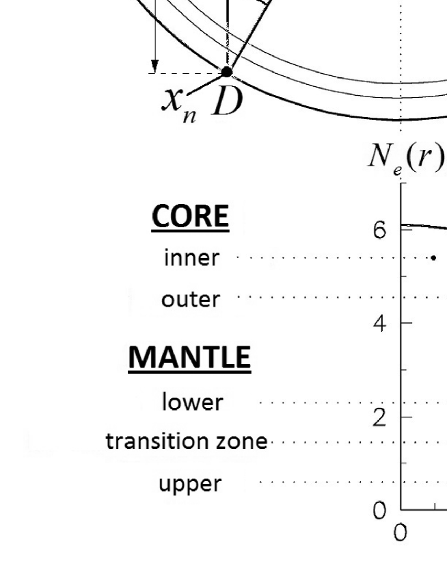
Figure 1: Radial distribution of the electron density $N_{e}(r)$ inside the Earth and the neutrino path through it. The figure demonstrates the cross section of the Earth which contains the nadir $DO$, the center of the Earth $O$, and the neutrino ray

Let us consider a neutrino traveling through the Earth, which, according to the PREM model Anderson , consists of a number of concentric spherical shells. The boundary between the valleys $x_{j}$ corresponds to the point where the neutrino crosses one of the interfaces between the Earth’s shells; let $r_{j}$ be the radius of this interface (see Fig. 1). Further, the distances $L_{n,j}^{\pm}$ between the detector and the points where the neutrino enters/leaves the interface with radius $r_{j}$ are functions of the ‘nadir angle’ $\Theta_{\text{N}}\in[0,\pi]$ defined as the angle between the direction to the Sun and the nadir in the point of the detector. In terms of the solar elevation angle $\Theta_{\text{s}}$ Astronomy , the nadir angle is $\Theta_{\text{N}}=\Theta_{\text{s}}+\pi/2$. The nadir angle, in turn, is a function of the Earth’s axial rotation angle $\tau\in[0,2\pi)$ (‘time of day’) and the orbital motion angle $\varsigma\in[0,2\pi)$ (‘season’). The dependence of the distances on the nadir angle is easily found to be

$$L_{n,j} = L_{n,j}^{\pm}(\Theta_{\text{N}})=r_{n}\cos\Theta_{\text{N}}\pm\sqrt{r_{j}^{2}-r_{n}^{2}\sin^{2}\Theta_{\text{N}}},$$ (40)

$$\Theta_{\text{N}} \leq \arcsin r_{j}/r_{n},$$ (41)

where the upper/lower signs in (40) correspond to the neutrino entering/leaving the interface $r_{j}$ (see Fig. 1). The inequality (41) ensures that the intersection of the neutrino ray with this interface exists.

In order to find the night average of the electron/muon neutrino observation probabilities, let us note some properties of expressions (39) and (40). First, the number of interfaces crossed by the neutrino is defined via the inequality (41), so the number of the valleys and, thus, the number of terms entering the sums in (39) are changing during the night. Therefore, the night average of Eq. (39) contains the sum over all interfaces $j$, with the average of the $j$th oscillating term involving ${\scriptstyle\Delta}\psi_{n,j}$ defined as follows:

$$\langle{F(\Theta_{\text{N}})e^{2\mathrm{i}{\scriptstyle\Delta}\psi_{n,j}}}\rangle_{\text{night}}=\int\limits_{\Theta_{\text{N}}(\tau)\leq\arcsin r_{j}/r_{n}}\!\!\!\!\!\!\!\!\!\!\!\!F(\Theta_{\text{N}}(\tau))e^{2\mathrm{i}{\scriptstyle\Delta}\psi_{n,j}(\Theta_{\text{N}}(\tau))}\;\frac{\mathrm{d}\tau}{{\scriptstyle\Delta}\tau_{\text{night}}}.$$ (42)

Here, $F(\Theta_{\text{N}})$ is some slowly changing function of the nadir angle and ${\scriptstyle\Delta}\tau_{\text{night}}$ is the total duration of the night in terms of the Earth’s axial rotation angle $\tau$, namely, the length of the segment where $\Theta_{\text{N}}(\tau)<\pi/2$ (the Sun is below the horizon).

Second, the duration of the night is, in turn, a function of the season $\varsigma$. On the equinox, e.g., ${\scriptstyle\Delta}\tau_{\text{night}}=\pi$, while on the winter solstice, ${\scriptstyle\Delta}\tau_{\text{night}}\to\max$. However, the summer nights are just as long as the opposite winter days, so that

$${\scriptstyle\Delta}\tau_{\text{night}}(\varsigma+\pi)=2\pi-{\scriptstyle\Delta}\tau_{\text{night}}(\varsigma),$$ (43)

and the total duration of the nights over all the year is exactly half the year. Therefore, the averaging over the year of $N_{\varsigma}$ days should involve the division by the total duration of the nights, i.e., $\pi N_{\varsigma}$. For $N_{\varsigma}\gg 1$, the summation over the nights can be replaced by the integration,

$$\langle{\ldots}\rangle_{\text{night,year}}=\frac{1}{N_{\varsigma}\pi}\sum\limits_{\varsigma=\varsigma_{k}}\int\mathrm{d}\tau(\ldots)\approx\frac{1}{2\pi^{2}}\int\limits_{0}^{2\pi}\mathrm{d}\varsigma\int\mathrm{d}\tau(\ldots),\qquad\varsigma_{k}=\frac{2\pi k}{N_{\varsigma}},k=1,\ldots,N_{\varsigma},$$ (44)

and the averaging formula for the terms containing the phase incursion ${\scriptstyle\Delta}\psi_{n,j}$ takes the form

$$\langle{F(\Theta_{\text{N}})e^{2\mathrm{i}{\scriptstyle\Delta}\psi_{n,j}}}\rangle_{\text{night,year}}=\frac{1}{2\pi^{2}}\int\limits_{0}^{2\pi}\mathrm{d}\varsigma\int\limits_{\Theta_{\text{N}}(\tau,\varsigma)\leq\arcsin r_{j}/r_{n}}\!\!\!\!\!\!\!\!\!\!\!\!\mathrm{d}\tau\;F(\Theta_{\text{N}}(\tau,\varsigma))\,e^{2\mathrm{i}{\scriptstyle\Delta}\psi_{n,j}(\Theta_{\text{N}}(\tau,\varsigma))}.$$ (45)

Now we are able to apply the stationary phase technique to such an integral containing the rapidly oscillating exponential. Indeed, let us use the expression, which is valid for smooth functions $f(x)$ and $S(x)$ defined on segment $[a,b]$ containing a single non-degenerate stationary point $x_{0}\in(a,b)$ such that $S^{\prime}(x_{0})=0$, $S^{\prime\prime}(x_{0})\neq 0$ StationaryPhase

$$\int\limits_{a}^{b}f(x)e^{\mathrm{i}\lambda S(x)}\mathrm{d}{x}=\sqrt{\frac{2\pi}{\lambda|S^{\prime\prime}(x_{0})|}}f(x_{0})e^{\mathrm{i}\lambda S(x_{0})+\mathrm{i}(\pi/4)\operatorname{sgn}S^{\prime\prime}(x_{0})}+\left.\frac{f(y)e^{\mathrm{i}\lambda S(y)}}{\mathrm{i}\lambda S^{\prime}(y)}\right|_{a}^{b}+\mathit{O}(\lambda^{-3/2}),\quad\lambda\to+\infty.$$ (46)

The two leading terms come from the stationary point and the boundary, respectively. However, in the application to the integral (42), the boundary term vanishes. Indeed, the boundary of the integration domain corresponds to the neutrino ray being tangent to the interface with radius $r_{j}$, hence, $\partial_{\tau}{\scriptstyle\Delta}\psi_{n,j}\propto\partial_{\tau}L_{n,j}(\Theta_{\text{N}}(\tau))\to\infty$, and the boundary term is absent. On the other hand, the stationary point is obviously achieved at midnight, when the nadir angle $\Theta_{\text{N}}\to\min$ (the Sun is in its lowest position), so the integration over the night yields

$$\int\limits_{\Theta_{\text{N}}(\tau)\leq\arcsin r_{j}/r_{n}}\!\!\!\!\!\!\!\!\!\!\!\!F(\Theta_{\text{N}}(\tau))\,e^{2\mathrm{i}{\scriptstyle\Delta}\psi_{n,j}(\Theta_{\text{N}}(\tau))}\;\frac{\mathrm{d}\tau}{\pi}=\left.\sqrt{\frac{1}{\pi\lambda|\partial_{\tau}^{2}L_{n,j}|}}F(\Theta_{\text{N}})e^{2\mathrm{i}{\scriptstyle\Delta}\psi_{n,j}\mp\mathrm{i}\pi/4}\right|_{\text{midnight}}+\mathit{O}((\lambda L_{n,j})^{-\frac{3}{2}}),$$ (47)

where the two possible signs before $\mathrm{i}\pi/4$ correspond to $L_{n,j}=L_{n,j}^{\pm}$ (see Eq. (40)). The principal point here is that the second derivative $\partial_{\tau}^{2}L_{n,j}$ at midnight is suppressed for the inner Earth’s shells,

$$\left[\partial_{\tau}^{2}L_{n,j}(\Theta_{\text{N}}(\tau))\right]_{\text{midnight}} = \left[\partial_{\tau}^{2}(\cos\Theta_{\text{N}})\frac{\mathrm{d}L_{n,j}(\Theta_{\text{N}})}{\mathrm{d}(\cos\Theta_{\text{N}})}\right]_{\text{midnight}},$$ (48)

$$\left[\frac{\mathrm{d}L_{n,j}(\Theta_{\text{N}})}{\mathrm{d}(\cos\Theta_{\text{N}})}\right]_{\text{midnight}} = \pm\left[\frac{L_{n,j}(\Theta_{\text{N}})}{\sqrt{r_{j}^{2}/r_{n}^{2}-\sin^{2}\Theta_{\text{N}}}}\right]_{\text{midnight}}.$$ (49)

Now let us use the expression of the nadir angle $\Theta_{\text{N}}$ via the Earth’s axial tilt $\varepsilon=23.5^{\circ}$, the latitude of the detector $\chi\in[-\pi/2,\pi/2]$, and the season $\varsigma\in[0,2\pi]$ Astronomy ,

$$\cos\Theta_{\text{N}}(\tau,\varsigma)=\cos\chi\sin\varsigma\sin\tau+\cos\varepsilon\cos\chi\cos\varsigma\cos\tau+\sin\varepsilon\sin\chi\cos\varsigma,$$ (50)

where $\varsigma=0$ corresponds to the winter solstice in the northern hemisphere. The minimum values of $\Theta_{\text{N}}$ are achieved at midnights corresponding to $\tau=\tau_{\text{midnight}}$,

$$\tan\tau_{\text{midnight}}(\varsigma)=\frac{\tan\varsigma}{\cos\varepsilon},\quad\cos\tau_{\text{midnight}}(\varsigma)=\operatorname{sgn}(\cos\varsigma)\frac{\cos\varepsilon}{\sqrt{\cos^{2}\varepsilon+\tan^{2}\varsigma}}.$$ (51)

Using these expressions, we find the derivative of $\cos\Theta_{\text{N}}$ at midnight,

$$\left[\partial_{\tau}^{2}(\cos\Theta_{\text{N}})\right]_{\text{midnight}}=-\frac{\cos\chi}{|\cos\varsigma|}\,\frac{\cos^{2}\varepsilon+\sin^{2}\varsigma\sin^{2}\varepsilon}{\sqrt{\cos^{2}\varepsilon+\tan^{2}\varsigma}}\equiv-\mathcal{N}(\varsigma).$$ (52)

Finally, the integral over the night (47) takes the form

$$\int\limits_{\Theta_{\text{N}}(\tau)\leq\arcsin r_{j}/r_{n}}\!\!\!\!\!\!\!\!\!\!\!\!F(\Theta_{\text{N}}(\tau))\,e^{2\mathrm{i}{\scriptstyle\Delta}\psi_{n,j}(\Theta_{\text{N}}(\tau))}\;\frac{\mathrm{d}\tau}{\pi}\approx\frac{1}{\sqrt{\mathcal{N}(\varsigma)}}\left[\frac{(r_{j}^{2}/r_{n}^{2}-\sin^{2}\Theta_{\text{N}})^{1/4}}{\sqrt{\pi\lambda L_{n,j}(\Theta_{\text{N}})}}F(\Theta_{\text{N}})e^{2\mathrm{i}{\scriptstyle\Delta}\psi_{n,j}\mp\mathrm{i}\pi/4}\right]_{\text{midnight}}.$$ (53)

On the other hand, the midnight stationary (minimum) values of the nadir angle $\Theta_{\text{N}}(\tau_{\text{midnight}})$ vary throughout the year (see Eq. (51)), being the smallest on the winter solstice (the darkest midnight) and the largest on the opposite summer solstice (the lightest midnight). Therefore, the right side of Eq. (53) is still containing a rapidly oscillating function of the season $\varsigma$, and we can perform another isolation of the stationary points, namely, of the two solstices $\varsigma=0,\pi$:

$$\langle{F(\Theta_{\text{N}})e^{2\mathrm{i}{\scriptstyle\Delta}\psi_{n,j}}}\rangle_{\text{night,year}}=\int\limits_{0}^{2\pi}\frac{\mathrm{d}\varsigma}{2\pi}\int\limits_{\Theta_{\text{N}}(\tau,\varsigma)\leq\arcsin r_{j}/r_{n}}\!\!\!\!\!\!\!\!\!\!\!\!F(\Theta_{\text{N}}(\tau,\varsigma))\,e^{2\mathrm{i}{\scriptstyle\Delta}\psi_{n,j}(\Theta_{\text{N}}(\tau,\varsigma))}\;\frac{\mathrm{d}\tau}{\pi}$$

$$=\frac{1}{2\pi}\sum\limits_{\varsigma=0,\pi}\frac{\vartheta\big{(}r_{j}-r_{n}\sin\Theta_{\text{N}}\big{)}}{\sqrt{\mathcal{N}(\varsigma)|\partial_{\varsigma}^{2}\cos\Theta_{\text{N}}(\tau_{\text{midnight}}(\varsigma))|}}\left[\frac{\sqrt{r_{j}^{2}/r_{n}^{2}-\sin^{2}\Theta_{\text{N}}}}{\lambda L_{n,j}(\Theta_{\text{N}})}F(\Theta_{\text{N}})e^{2\mathrm{i}{\scriptstyle\Delta}\psi_{n,j}+\mathrm{i}s^{\prime}(s-1)\pi/4}\right]_{\text{midnight}},$$ (54)

$$\partial_{\varsigma}^{2}\cos\Theta_{\text{N}}(\tau_{\text{midnight}}(\varsigma))=\begin{cases}\sin(\varepsilon-\chi)\tan\varepsilon,&\varsigma=0\text{ (winter solstice),}\\ \sin(\varepsilon+\chi)\tan\varepsilon,&\varsigma=\pi\text{ (summer solstice),}\end{cases}$$ (55)

$$s\equiv\operatorname{sgn}\bigl{\{}\partial_{\varsigma}^{2}\cos\Theta_{\text{N}}(\tau_{\text{midnight}}(\varsigma))\bigr{\}}=\begin{cases}-1,&\varsigma=0,\\ +1,&\varsigma=\pi,\end{cases}$$ (56)

$$s^{\prime}=\operatorname{sgn}\bigl{\{}L_{n,j}(\Theta_{\text{N}})-r_{n}\cos\Theta_{\text{N}}\bigr{\}}=\pm 1\qquad\text{for }L_{n,j}=L_{n,j}^{\pm},$$ (57)

$$\vartheta(\xi)\equiv\begin{cases}1,&\xi\geq 0,\\ 0,&\xi<0.\end{cases}$$ (58)

In the above expressions, the Heaviside theta function $\vartheta\big{(}r_{j}-r_{n}\sin\Theta_{\text{N}}\big{)}$ ensures that the stationary point for the $j$th interface is really reached, while the additional sign $s^{\prime}$ is explicitly introduced to avoid $\pm$-expressions originating from Eq. (40). The signs specified in Eq. (54) are valid in the northern non-tropical and non-polar latitudes $\chi\in(\varepsilon,\pi/2-\varepsilon)$. Indeed, the typical neutrino detectors (SNO, Borexino, Super-Kamiokande) are situated in temperate latitudes. Here, the midnight solstice nadir angle is $\Theta_{\text{N}}(\tau_{\text{midnight}})=\chi+s\varepsilon$ and the prefactor $\mathcal{N}(\varsigma)=\cos\varepsilon\cos\chi$. With the use of this fact together with the above general averaging formula, one finally arrives at the year average of the night transition probability (39),

$$\langle{T_{\text{night}}}\rangle_{\text{night,year}} \approx \cos 2\theta_{\text{Sun}}\cos 2\theta_{n}^{-}+2\cos 2\theta_{\text{Sun}}\sin 2\theta_{n}^{-}\sum\limits_{j=1}^{n-1}{\scriptstyle\Delta}\theta_{j}$$ (59)

$$\times \sum\limits_{s=\pm 1}\frac{\vartheta\big{(}r_{j}-r_{n}\sin(\chi+s\varepsilon)\big{)}}{2\pi\sqrt{\sin\varepsilon\cos\chi\sin(\chi+s\varepsilon)}}\frac{\sqrt{r_{j}^{2}/r_{n}^{2}-\sin^{2}(\chi+s\varepsilon)}}{\lambda L_{n,j}(\chi+s\varepsilon)}\cos\{2{\scriptstyle\Delta}\psi_{n,j}+s^{\prime}(s-1)\pi/4\},$$

$$s^{\prime} \equiv \operatorname{sgn}\{L_{n,j}(\chi+s\varepsilon)-r_{n}\cos(\chi+s\varepsilon)\}.$$ (60)

In the above expression, we have omitted the terms resulting from averaging the $\mathit{O}(\eta\delta)$ terms in Eq. (39), since they are extremely small. The phase incursions ${\scriptstyle\Delta}\psi_{n,j}$ should obviously be taken at $\Theta_{\text{N}}=\chi+s\varepsilon$, i.e. at solstice midnights. For the Borexino detector situated in the Gran Sasso laboratory, with $\theta=+42.5^{\circ}$, the prefactor in (59) which does not depend on $j$ amounts to be

$$\frac{1}{2\pi\sqrt{\sin\varepsilon\cos\chi\sin(\chi+s\varepsilon)}}\approx\begin{cases}0.51,&\text{ winter solstice ($s=-1$)},\\ 0.31,&\text{ summer solstice ($s=+1$)}.\end{cases}$$ (61)

For the Super-Kamiokande detector, $\theta=+36.2^{\circ}$, and the prefactor equals $0.60$ and $0.30$ for the two stationary points, respectively.

Let us briefly note that, in the tropical latitudes $|\chi|<\varepsilon$, additional stationary points appear; in particular, on the Equator $\chi=0$, they correspond to the equinoxes. Two additional points meet on the winter solstice, when $\chi\to+\varepsilon$ (on the Tropic), and one encounters a degenerate stationary point StationaryPhase . Although we have found the analytical expressions for the year averages in the tropical and equatorial zones ($|\chi|\leq\varepsilon$), we do not present them here due to their mathematical complexity and to the fact that the actual neutrino detectors are situated in the temperate latitudes. We confine ourselves to saying that, from (61), one can infer the amplification of the winter solstice contribution, as one approaches the Tropic.

One should also mention that, for low-energy neutrinos ($E\lesssim 1~{}\text{MeV}$), in certain seasons, the phase incursions ${\scriptstyle\Delta}\psi_{n,j}$ for a certain layer $j$ may differ by approximately a multiple of $2\pi$ on the successive nights. As a result, the contributions of these nights will not cancel each other, quite similarly to those of the nights near the solstices. This may be called a parametric resonance and, in principle, will lead to local anomalies in the observed neutrino flux, but, as one may see from Sec. IV, the day-night asymmetry for low-energy neutrinos is quite small and its anomalies are even more challenging to observe. Thus, we do not pay these additional effects much attention here.

Finally, we are left with the following conclusion. The terms entering Eq. (39), which contain the oscillating functions of the phase incursions $2{\scriptstyle\Delta}\psi_{n,j}$, are suppressed as $\mathit{O}\left(\frac{r_{j}}{r_{n}\lambda L_{n,j}}\right)=\mathit{O}\left(\frac{r_{j}}{r_{n}}\delta\right)$ after averaging over the year; within the leading approximation, the resulting averages (59) come from the stationary phase points achieved on the winter and the summer solstices. The suppression becomes stronger for the inner Earth’s shells.

It is spectacular that all the terms of the order $\mathit{O}(\eta\delta)$ in the expression (39), including the one corresponding to the detector, become $\mathit{O}(\eta\delta^{2}r_{j}/r_{n})$ after the averaging. The terms of the order $\mathit{O}(\eta)$, which are proportional to ${\scriptstyle\Delta}\theta_{j}$, become $\mathit{O}(\eta\delta r_{j}/r_{n})$, respectively. Finally, we are left with the average value

$$\langle{T_{\text{night}}}\rangle=\cos 2\theta_{\text{Sun}}\cos 2\theta_{n}^{-}+\mathit{O}\left(n\eta\delta\frac{r_{j}}{r_{n}}\right).$$ (62)

By substituting this result together with the daytime average value (33) into expression (27) for the neutrino observation probabilities, we arrive at the day-night asymmetry factor

$$A_{\text{dn}}\equiv\frac{2(\langle{P_{e,\text{night}}}\rangle-\langle{P_{e,\text{day}}}\rangle)}{\langle{P_{e,\text{night}}}\rangle+\langle{P_{e,\text{day}}}\rangle}=-\frac{T_{\text{MSW}}}{1+T_{\text{MSW}}}\cdot\frac{\sin^{2}2\theta_{0}}{\cos 2\theta_{0}}\frac{2EV(x_{n}^{-})}{{\scriptstyle\Delta}m^{2}}+\mathit{O}\left(n\eta\delta\frac{r_{j}}{r_{n}}\right),$$ (63)

where $T_{\text{MSW}}=\cos 2\theta_{0}\cos 2\theta_{\text{Sun}}={a_{\text{vac}}a_{\text{Sun}}}/{\omega_{\text{Sun}}}$ defines the observation probabilities for the solar neutrinos due to the Mikheev–Smirnov–Wolfenstein effect MikheevSmirnov and $V(x_{n}^{-})$ is the Wolfenstein potential in the Earth under the detector.

One should hold in mind that the asymmetry factor defined as (63) may not be directly measurable in the neutrino experiments, depending on the detection mechanism. Indeed, definition (63) differs from the one preferred by the experimentalists, the latter being

$$A_{\text{dn}}^{\text{(exp)}}=\frac{2(N_{\text{night}}-N_{\text{day}})}{N_{\text{night}}+N_{\text{day}}},$$ (64)

where $N_{\text{day,night}}$ is the number of neutrino events observed during the day/night. These numbers may not correspond to the electron neutrino fluxes. For example, scattering experiments, which cannot separate the charged and the neutral current interactions, are unable to directly measure the electron neutrino flux. To compare prediction (63) with such experiments, one should reinterpret the observed event rates $N_{\text{day,night}}$ in terms of the electron neutrino fluxes using some theoretical assumptions.

Let us provide an example of the connection between the day-night asymmetry factors defined as (63) and (64). Namely, in the case of the neutrino-electron scattering experiment, such as Borexino, the incident neutrinos produce recoil electrons inside the detector, and the scattering cross sections for such processes are well-known Nu_e_CrossSection ; Bahcall_CrossSections , including one-loop corrections Nu_e_RadCorr . The resulting ratio of the total electron/muon neutrino detection cross sections is a function of the neutrino energy $E$ (as well as of the threshold $T_{\text{min}}$ of the recoil electron detection). For monochromatic beryllium neutrinos and the actual Borexino’s threshold, this ratio is Borexino1

$$\sigma(\nu_{e};E)/\sigma(\nu_{\mu};E)\approx 4.5,\qquad E=0.862~{}\text{MeV},$$ (65)

thus, the ratio of the event rates is

$$\frac{N_{\text{day}}}{N_{\text{night}}}=\frac{\langle{P_{e,\text{day}}}\rangle\sigma(\nu_{e})+(1-\langle{P_{e,\text{day}}}\rangle)\sigma(\nu_{\mu})}{\langle{P_{e,\text{night}}}\rangle\sigma(\nu_{e})+(1-\langle{P_{e,\text{night}}}\rangle)\sigma(\nu_{\mu})}.$$ (66)

The ‘experimental’ day-night asymmetry factor is then easily found to be

$$A_{\text{dn}}^{\text{(exp)}}\approx A_{\text{dn}}\;\frac{(\sigma(\nu_{e})-\sigma(\nu_{\mu}))(1+T_{\text{MSW}})}{(\sigma(\nu_{e})-\sigma(\nu_{\mu}))(1+T_{\text{MSW}})+2\sigma(\nu_{\mu})}$$ (67)

and, for beryllium neutrinos ($T_{\text{MSW}}\approx 0.09$), we obtain

$$A_{\text{dn}}^{\text{(exp)}}\approx 0.66A_{\text{dn}}\qquad(E=0.862~{}\text{MeV}).$$ (68)

For boron and other types of neutrinos, which have continuous energy spectrum, the expression for the ‘experimental’ day-night asymmetry factor involves the integration over the neutrino energy,

$$A_{\text{dn}}^{\text{(exp)}}=\frac{\int\rho(E)\mathrm{d}{E}\times A_{\text{dn}}(E)\;(\sigma(\nu_{e};E)-\sigma(\nu_{\mu};E))(1+T_{\text{MSW}}(E))}{\int\rho(E)\mathrm{d}{E}\times\{(\sigma(\nu_{e};E)-\sigma(\nu_{\mu};E))(1+T_{\text{MSW}}(E))+2\sigma(\nu_{\mu};E)\}}.$$ (69)

Here, the cross sections $\sigma(\nu_{e,\mu};E)$, the ‘physical’ asymmetry factor $A_{\text{dn}}$, and the Mikheev–Smirnov–Wolfenstein factor $T_{\text{MSW}}$ depend on the neutrino energy, and $\rho(E)$ is the normalized energy distribution of incident neutrinos. As one can see, the integration can be easily undertaken numerically using our asymmetry prediction (63) and the expressions for the effective total cross sections, if the recoil electron detection threshold $T_{\text{min}}$ is known (see, e.g., Bahcall_CrossSections ).

For those experiments which directly observe the charged-current electron neutrino events, one formally sets $\sigma(\nu_{\mu};E)\to 0$. Then one has $A_{\text{dn}}^{\text{(exp)}}=A_{\text{dn}}$ for monochromatic neutrinos and

$$A_{\text{dn}}^{\text{(exp)}}=\frac{\int\rho(E)\sigma(\nu_{e};E)\mathrm{d}{E}\times A_{\text{dn}}(E)\;(1+T_{\text{MSW}}(E))}{\int\rho(E)\sigma(\nu_{e};E)\mathrm{d}{E}\times(1+T_{\text{MSW}}(E))}\qquad\text{(charged current only)}$$ (70)

for continuous-spectrum neutrinos.

III.3 The effect of the crust

The estimation (63) shown above is substantially based on the piecewise continuous structure of the density profile and shows that the asymmetry should depend only on the density of rock immediately under the detector, i.e. in the Earth’s crust. At the same time, for beryllium neutrinos, the actual width of the crust is comparable with the oscillation length, and neither the valley nor the cliff approximation is valid for this layer. For boron neutrinos, the crust can be considered a cliff, however, the oscillation length becomes comparable with the thickness of the upper mantle, as well as with thicknesses of transition zones (see Fig. 1 and Anderson1 ). Moreover, the phase incursions are small within the crust (and the upper mantle), and so are their time variations, hence, we are unable to use the stationary phase approximation. However, we are still able to account for the effect of these near-surface layers on the observed day-night asymmetry factor (63), relying upon relatively small density variation ${\scriptstyle\Delta}\eta$ within them. This feature, together with the bounded layers’ thickness, makes it possible to find the closed form of the approximate flavor evolution operator for the crust (the upper mantle) $[x_{n-1}^{+},x_{n}^{-}]$  (see Appendix A.4),

$$R_{0}(x_{n}^{-},x_{n-1}^{+}) = \exp\{(-\mathrm{i}\sigma_{2}\beta+\mathrm{i}\sigma_{1}\alpha)e^{2\mathrm{i}\sigma_{3}\psi(x_{n-1}^{+})}\}+\mathit{O}(\eta^{2}),$$ (71)

$$\beta+\mathrm{i}\alpha = \int\limits_{x_{n-1}^{+}}^{x_{n}^{-}}\dot{\theta}(y)e^{2\mathrm{i}(\psi(y)-\psi(x_{n-1}^{+}))}\mathrm{d}{y},\qquad\alpha,\beta=\mathit{O}({\scriptstyle\Delta}\eta)\in\mathds{R}.$$ (72)

This result formally repeats the cliff approximation (19) up to the substitution ${\scriptstyle\Delta}\theta_{j}\to\beta$, $\mu_{j}\to\alpha$. Using such a substitution, the transition zones, whose widths are comparable with the boron neutrino oscillation lengths, can be safely replaced by the cliffs, preserving the form of expression (39). Finally, to account for the effect of the crust (and the upper mantle), as well as the effects of the transition zones, we should make the following modification in (39):

$$T_{\text{night}} = \cos 2\theta_{\text{Sun}}\Bigl{\{}\cos 2\theta_{n}^{-}+2\sin 2\theta_{n}^{-}\sum_{j=1}^{n-1}({\scriptstyle\Delta}\theta_{j}\cos 2{\scriptstyle\Delta}\psi_{n,j}+\bar{\mu}_{j}\sin 2{\scriptstyle\Delta}\psi_{n,j})$$ (73)

$$\qquad\qquad-4{\scriptstyle\Delta}\psi_{\text{det}}\sin 2\theta_{\text{det}}\sum_{j=1}^{n-1}{\scriptstyle\Delta}\theta_{j}\sin 2{\scriptstyle\Delta}\psi_{n,j}\Bigr{\}}+{\scriptstyle\Delta}T_{\text{night}},$$

$${\scriptstyle\Delta}T_{\text{night}} = \cos 2\theta_{\text{Sun}}\{2\sin 2\theta_{n}^{-}(\beta\cos 2{\scriptstyle\Delta}\psi_{n,n-1}+\alpha\sin 2{\scriptstyle\Delta}\psi_{n,n-1})$$ (74)

$$\qquad\qquad-4{\scriptstyle\Delta}\psi_{\text{det}}\sin 2\theta_{\text{det}}(\beta\sin 2{\scriptstyle\Delta}\psi_{n,n-1}-\alpha\cos 2{\scriptstyle\Delta}\psi_{n,n-1})\}$$

$$= 2\cos 2\theta_{\text{Sun}}\sin 2\theta_{n}^{-}\int\limits_{x_{n-1}^{+}}^{x_{n}^{-}}\dot{\theta}(y)\cos 2{\scriptstyle\Delta}\psi(y)\;\mathrm{d}{y}-4\cos 2\theta_{\text{Sun}}{\scriptstyle\Delta}\psi_{\text{det}}\sin 2\theta_{\text{det}}\int\limits_{x_{n-1}^{+}}^{x_{n}^{-}}\dot{\theta}(y)\sin 2{\scriptstyle\Delta}\psi(y)\;\mathrm{d}{y},$$

where ${\scriptstyle\Delta}\psi(y)\equiv\psi(x_{n}^{-})-\psi(y)$. The leading $\mathit{O}(\eta)$ correction of the crust (the upper mantle) to the day-night asymmetry factor (63) reads

$${\scriptstyle\Delta}A_{\text{dn}}=\frac{T_{\text{MSW}}}{1+T_{\text{MSW}}}\cdot\frac{\sin^{2}2\theta_{0}}{\cos 2\theta_{0}}\frac{2E}{{\scriptstyle\Delta}m^{2}}\int\limits_{x_{n-1}^{+}}^{x_{n}^{-}}\dot{V}(y)\cos 2{\scriptstyle\Delta}\psi(y)\,\mathrm{d}{y}.$$ (75)

Again, this result should be subjected to the averaging procedure to acquire the predictive power. However, due to the boundedness of the cosine, the correction is easily estimated (both before and after averaging),

$$\left|\frac{({\scriptstyle\Delta}A_{\text{dn}})}{A_{\text{dn}}}\right|\leq\frac{1}{V(x_{n}^{-})}\int\limits_{x_{n-1}^{+}}^{x_{n}^{-}}|\dot{V}(y)|\mathrm{d}{y}\sim\frac{|({\scriptstyle\Delta}V)_{\text{crust}}|}{V(x_{n}^{-})}.$$ (76)

IV Discussion

Let us begin with the review of the approximations we were using in the above calculations of the day-night asymmetry. First, the Sun was considered one big valley, i.e. the adiabatic approximation was used for it. The non-adiabatic corrections are of the order of the adiabaticity parameter $\gamma=|\dot{\theta}(x)|/\lambda\omega$ MikheevSmirnov . Using the fact that the typical spatial scale of the solar density variation is associated with the solar core radius $R_{0}\sim 0.1R_{\text{Sun}}\approx 7\times 10^{4}~{}\text{km}$ SolarDensity , we find

$$\gamma_{\text{Sun}}\lesssim\begin{cases}10^{-5},&\quad E\sim 1~{}\text{MeV},\\ 5\times 10^{-4},&\quad E\sim 10~{}\text{MeV}.\end{cases}$$ (77)

Thus, these corrections can be safely neglected.

Neglecting the finite width of the detector introduces a relative error of the order $\mathit{O}\left(\frac{L_{\text{det}}}{\ell_{\text{osc}}}\ \delta\right)$, compared with the leading term (63), as one can see from (39). This correction is minuscule even for beryllium neutrinos ($\ell_{\text{osc}}\approx 30~{}\text{km}$), since the detector sizes are now $L_{\text{det}}\leq 1~{}\text{km}$. Moreover, this type of correction is subjected to additional suppression due to time averaging.

The valley-crust approximation considered in Sec. II relies upon the smallness of parameters $\eta$ and $\delta$. The relative error of the linear approximation in $\eta$ is of the order of $\mathit{O}(\eta)$, hence, this approximation works fine for beryllium neutrinos and quite well for boron neutrinos (see Eq. (7); note that the maximum values specified for $\eta$ correspond to the inner core, while for typical neutrino detector latitudes, the Sun never descends low enough to shine through it). Thus, for boron neutrinos, the error of the linear approximation is within $10\%$. Further, the error due to the finite width of the $j$th valley is estimated as $\mathit{O}({\scriptstyle\Delta}\eta_{j}\delta_{j})=\mathit{O}({\scriptstyle\Delta}\eta_{j}\ \ell_{\text{osc}}/L_{j})$, where ${\scriptstyle\Delta}\eta_{j}$ is the density variation on the $j$th valley and $L_{j}$ is the width of the valley. On the other hand, if the width of the $k$th cliff $L_{k}\not\ll\ell_{\text{osc}}$, the resulting error is $\mathit{O}(\eta\delta_{k})=\mathit{O}(\eta\ L_{k}/\ell_{\text{osc}})$. Within the PREM model, the cliffs are abrupt ($\delta_{k}=0$), so we will not discuss the numerical values of the corresponding errors.

If there are deep layers in the PREM density distribution, whose widths are of the order of the oscillation length, they can be considered neither valleys nor cliffs. However, if the density variations ${\scriptstyle\Delta}\eta$ over these layers are small, we can use the approximation considered in Sec. III.3 and Appendix A.4, which formally reduces these layers to the cliffs (see Eq. (71)). The error of such an approach is measured by the magnitudes of parameters $\alpha,\beta$ in (71), i.e. the error is of the order of ${\scriptstyle\Delta}\eta$. The contributions of such layers are additionally suppressed after averaging, due to their depth (see below). In the case of the Earth, there is a layer of this type. Namely, the core-mantle transition zone is about $200\,\text{km}$ wide Anderson1 , which is of the order of the typical boron neutrino oscillation length. However, the corresponding density variation lies within only ${\scriptstyle\Delta}\eta/\eta\sim 5-7\%$, and the time-averaged contribution is obviously negligible. For beryllium neutrinos, the core-mantle transition zone can be considered a valley.

The contributions from the Earth’s layers, which lie much more than the oscillation length under the detector, are suppressed due to time averaging, the principal nonvanishing contributions being provided by the winter/summer solstice stationary points. These contributions have the relative magnitude $\mathit{O}\left(\frac{{\scriptstyle\Delta}\theta_{j}}{{\scriptstyle\Delta}\theta_{n}}\frac{r_{j}}{r_{n}}\frac{\ell_{\text{osc}}}{L_{n,j}}\right)$ compared with the leading term (63)  (see Eqs. (39) and (59)). This suppression is quite strong for dense though deep inner Earth’s shells, including its core.

Finally, for the layers which lie within $\mathit{O}(\ell_{\text{osc}})$ under the detector and have the widths comparable with the oscillation length, the averaging procedure cannot be performed so as to result in the expression (59). Here, we are only able to follow the approach of Sec. (III.3), which results in an unaveraged correction (75). The latter correction, in principle, can be explicitly averaged using numerical integration, which in this case involves only the near-surface Earth’s structure. The strict constraint on the uncertainty introduced by neglecting the effect of this structure is given in Eq. (76). This expression predicts the $20\%$ uncertainty for beryllium and $\sim 30\%$ for boron neutrinos. However, it is quite obvious that the time average of the cosine in (75) is sensitive to the Wolfenstein potential in the layers within $\mathit{O}(\ell_{\text{osc}})$ under the detector; moreover, (59) shows that this sensitivity asymptotically falls off as the inverse depth of the layer $L_{n,j}$. Thus, if the resulting expression (63) is used for boron neutrinos, one should substitute for $V(x_{n}^{-})$ the Wolfenstein potential averaged over the crust and the uppermost layers of the mantle, using some decreasing weighting function. The resulting potential will be $15-20\%$ larger than that immediately under the Earth’s surface. For beryllium neutrinos, it suffices to substitute the Wolfenstein potential in the crust.

Thus, we may conclude that, according to (63) and (75), the asymmetry has the order $\mathit{O}(\eta)$ and is determined by the rock density in the layer of width about $\ell_{\text{osc}}$ under the detector, i.e. in the Earth’s crust (as well as in the uppermost part of the mantle for boron neutrinos). The principal uncertainty of expression (63) comes from the fact that the stationary point approximation we used for the analytical time averaging of Eq. (39) is inapplicable to the layers which lie within several neutrino oscillation lengths under the detector. Another correction comes from the time averaging of oscillating contributions of the deep layers; using (59), we can estimate its magnitude as $\leq 3\%$ for beryllium neutrinos and $\leq 10-15\%$ for boron neutrinos with $E=10~{}\text{MeV}$. All other corrections, taken together, do not exceed $10\%$.

Using the recent data from SNO, KamLAND, and Borexino collaborations SNO ; KamLand ; Borexino1 , namely, $\tan^{2}\theta_{0}\approx 0.46$ and ${\scriptstyle\Delta}m^{2}\approx 7.6\times 10^{-5}~{}\text{eV}^{2}$, and the typical electron densities in the Earth’s crust $N_{e(\text{crust})}=1.3\,\text{mol}/\text{cm}^{3}$ Anderson1 and in the solar core $N_{e(\text{Sun})}\sim 100~{}\text{mol}/\text{cm}^{3}$ SolarDensity , we arrive at the numerical estimation for the day-night asymmetry factor for solar beryllium-7 neutrinos ($E=0.862\,\text{MeV}$)

$$A_{\text{dn}}({}^{7}\text{Be})=(-4.0\pm 0.9)\times 10^{-4},\qquad A_{\text{dn}}^{\text{(exp)}}({}^{7}\text{Be})=(-2.6\pm 0.6)\times 10^{-4}.$$ (78)

The uncertainty corresponds to the effect of the Earth’s crust, which, as mentioned, can be explicitly evaluated by numerical averaging of Eq. (75). For boron-8 neutrinos with $E=10~{}\text{MeV}$, substitution of the crust density into (63) leads to the asymmetry estimation

$$A_{\text{dn}}({}^{8}\text{B})\approx(2.9\pm 0.8)\times 10^{-2}\qquad(E=10\text{~{}MeV}).$$ (79)

The ‘experimental’ asymmetry factor for the electron scattering experiment with the recoil kinetic energy threshold $T_{\text{min}}=4.5\text{~{}MeV}$ (such as Super-Kamiokande-III SuperKIII_2010 ), averaged over boron-8 solar neutrino spectrum Boron8Spectrum , is then given by Eq. (69),

$$A_{\text{dn}}^{\text{(exp)}}({}^{8}\text{B})\approx(1.6\pm 0.5)\times 10^{-2}\qquad\text{(averaged over energy)},$$ (80)

the fully-numerical calculation yielding $A_{\text{dn}}^{\text{(exp)}}({}^{8}\text{B})=1.9\times 10^{-2}$. We do not present here the asymmetry predictions for ${}^{13}\text{N}$, ${}^{15}\text{O}$, and $pep$ neutrinos, since their typical energies are around $1\text{~{}MeV}$, while the fluxes at least one order smaller than that for beryllium neutrinos SolarDensity .

If, for boron neutrinos, one substitutes into (63) the mean density in the near-surface layers, instead of the crust density, the above predictions (79), (80) will be about 10% larger (depending on the weighting function chosen for the mean density evaluation) but never larger than those obtained by substituting the density of the upper mantle. Indeed, Fig. 2b shows that the two analytical curves corresponding to the two ‘surface densities’ discussed here enclose the fits obtained using two techniques of numerical simulation. One of these simulations involves the numerical time averaging of the leading $\mathit{O}(\eta)$ terms in expression (39) (the valley-cliff approximation), while the other one includes both the numerical solution of the evolution equation (14) and the subsequent time averaging.

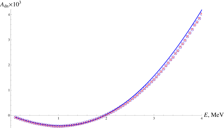
(a)


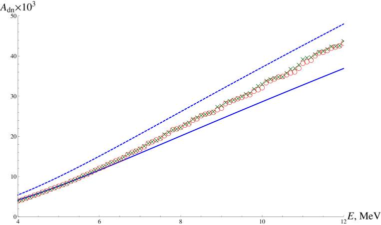
(b)

Figure 2: Comparison of analytical expression (63) for the day-night asymmetry factor with the results of numerical simulations for Gran Sasso ($\chi=+42.5^{\circ}$). Solid/dashed curves: Analytical estimations (63) with the crust/upper mantle electron densities substituted; Circles ($\bigcirc$): The result based on numerical averaging of analytical expression (39) (‘valley-cliff’ approximation); Crosses ($\times$): Fully numerical result (numerical solution of (14) and subsequent numerical averaging). Subfigures (a) and (b) demonstrate the low- and high-energy segments of the curves, respectively.

The numerical curves shown in Fig. 2 were calculated for the Gran Sasso laboratory, where the Borexino detector is operating; the curves for Kamioka (Super-Kamiokande) and Sudbury (SNO) lie very close to that for Gran Sasso, so we do not show them in this figure. Instead, a comparison of numerical results for selected detector latitudes is presented in Fig. 3 (again, we do not include the SNO latitude, since the results for it lie very close to those for Gran Sasso). We have also included in Fig. 3 the numerical results for the Northern tropic, since, according to our analytical estimations, near it, the subleading contributions to the asymmetry may become considerable, which come from the solstices (see Eq. (59)). We will address this issue further in this section.

From Fig. 3, one may infer that the leading-order analytical estimation (63) is in good agreement with the numerical results even for boron neutrinos. Contrary to these numerical results, however, our analytical estimation is model-independent, in particular, it does not contain the latitude of the neutrino detector. The possible errors of our predictions can also be easily estimated. In the case of beryllium neutrinos, the estimation of the errors becomes strict enough to result in a fixed-boundary interval (not a confidence interval) for the day-night asymmetry shown in Eq. (78), which is useful for experimental purposes. Our results are also in agreement with numerical day-night asymmetry predictions presented by other authors (see, e.g., BahcallKrastev ).

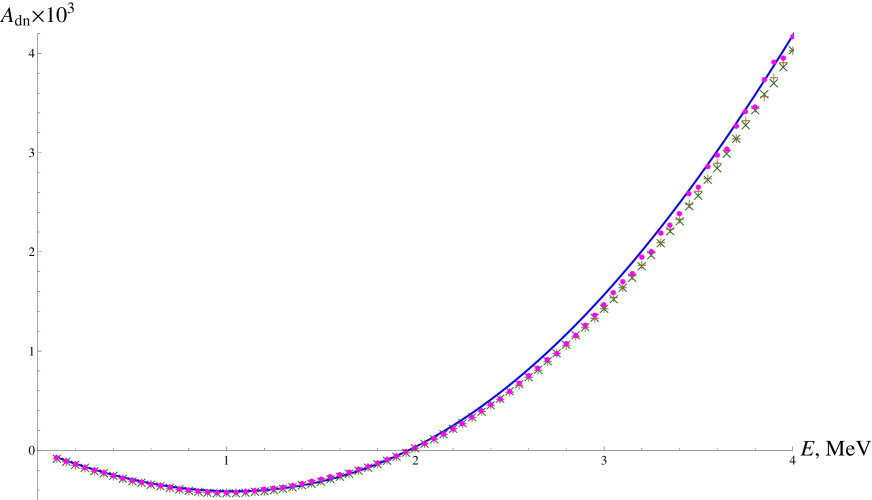
(a)


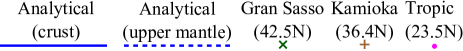
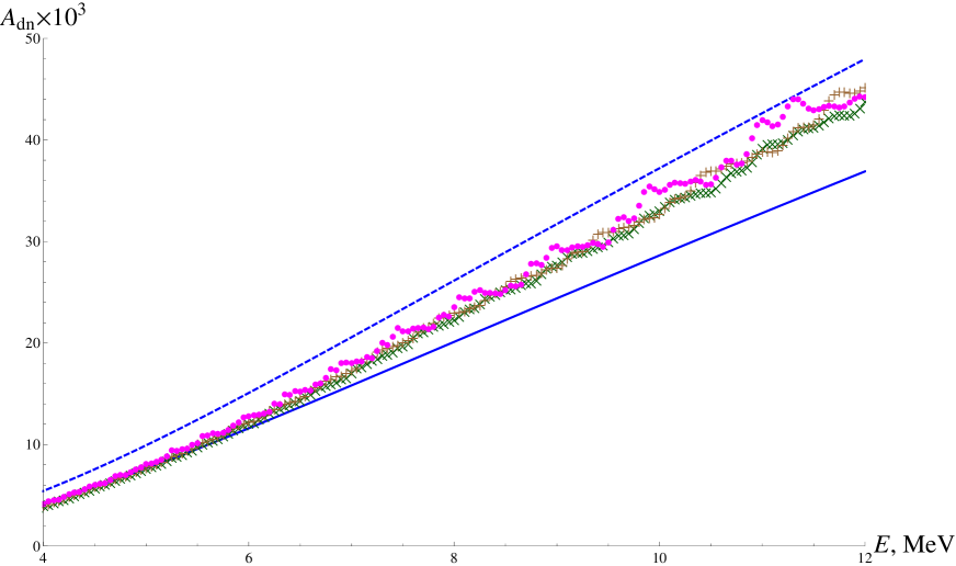
(b)

Figure 3: Comparison of analytical expression (63) for the day-night asymmetry factor with the results of numerical simulations for different detector latitudes. Solid/dashed curves: Analytical estimations (63) with the crust/upper mantle electron densities substituted; Crosses ($\times$): numerical result for Gran Sasso ($\chi=+42.5^{\circ}$), Pluses ($+$): for Kamioka ($\chi=+36.4^{\circ}$), Bullets ($\bullet$): for the Northern tropic ($\chi=+23.5^{\circ}$). Subfigures (a) and (b) demonstrate the low- and high-energy segments of the curves, respectively.

As predicted, the agreement of the numerical results with the analytical one becomes better for low-energy neutrinos. We also observe that the asymmetry vanishes for low-energy neutrinos, which is a result of the applicability of the adiabatic approximation for such neutrinos. Indeed, within this approximation, the neutrino flavor observation probabilities depend only on the creation and absorption points.

It is worth emphasizing here that such a directly measurable quantity, as the day-night asymmetry factor, does depend both on the neutrino regeneration effect inside the Earth and on the Mikheev–Smirnov–Wolfenstein effect inside the solar core, where the neutrino is created. Another useful physical quantity, namely, the regeneration factor $f_{\text{reg}}$, describes solely the Earth effect in the day-night asymmetry Wei ,

$$A_{\text{dn}} = -\frac{2\cos{2\theta_{\text{Sun}}}}{1+(T_{\text{night}}+T_{\text{day}})/2}f_{\text{reg}}\approx-\frac{2\cos{2\theta_{\text{Sun}}}}{1+T_{\text{MSW}}}f_{\text{reg}},$$ (81)

$$f_{\text{reg}} \approx \frac{1}{2}\sin^{2}2\theta_{0}\frac{2EV(x_{n}^{-})}{{\scriptstyle\Delta}m^{2}}.$$ (82)

Indeed, one observes that, unlike the regeneration factor (82), the day-night asymmetry (63) depends on the solar effect manifested in the energy-dependent quantity $T_{\text{MSW}}$. As a result, at the energy $E\sim 2.0\,\text{MeV}$, which corresponds to the Mikheev–Smirnov resonance in the solar core, we have $\cos 2\theta_{\text{Sun}}=0$ and $T_{\text{MSW}}=0$, and, as a consequence, the day-night asymmetry factor (63) changes sign (see Fig. 2a); on the other hand, the regeneration factor is always positive. Thus, it is the resonance inside the Sun which makes the asymmetry, observed on the Earth, vanish.

From Fig. 2a, 3a, one may observe that beryllium neutrinos ($E=0.862\,\text{MeV}$) would be indeed quite useful for the study of the matter effects in the neutrino oscillations, since they correspond to almost maximum asymmetry magnitude in the unusual domain of its negativity. Moreover, solar beryllium neutrinos are highly monochromatic (in contrast, e.g., to the boron neutrinos) and their flux is considerably larger SolarDensity . However, we are able to conclude that the day-night effect needs at least a 10–20 times improvement of current experimental resolution to be distinguished at a considerable confidence level for such neutrinos. In particular, the result of the Borexino experiment $A^{(\text{exp})}_{\text{dn}}({}^{7}\text{Be})=\bigl{(}1\pm 12\text{(stat.)}\pm 7\text{(syst.)}\bigr{)}\times 10^{-3}$ was reported in April, 2011 Borexino and demonstrates the strong dominance of the uncertainties over the expected effect. One may still hope that the 50 kton LENA detector which should come into operation around 2020 LENA and is expected to observe as much as $10^{4}$ solar beryllium neutrino events per day, could distinguish the day-night effect for such neutrinos. Strictly speaking, the Poisson statistics results in the relative errors $\Delta N/N\sim 1/\sqrt{N}$, and, for a year-long experiment, one reaches the statistical error of the order of $1/\sqrt{365\cdot 10^{4}}\sim 0.5\times 10^{-3}$. However, one could employ the adaptive processing of the experimental data, taking into account the expected form of the curve $T_{\text{night}}(\Theta_{\text{N}})$ (see (39) and (40)), i.e. the dependence of the asymmetry on the nadir angle. This processing technique may be efficient in extracting the day-night effect from under the noise even for small event rates. Quite a similar technique was recently suggested in LENA_FluxVariations as a search tool for periodic time variations in the ${}^{7}\text{Be}$ solar neutrino flux observed at LENA.

In Fig. 3b, one can also observe the role of the stationary phase points in the time average of the day-night asymmetry factor. Namely, the numerical curve corresponding to the Northern tropic demonstrates specific oscillations which come from the amplified contribution of the winter solstice stationary point to the year average of the asymmetry factor (see Eq. (59)). The curve for the Kamioka mine, which is situated about 1.5 times closer to the Tropic than Gran Sasso, also demonstrates oscillations, compared to the Gran Sasso curve. In view of this effect, it would be quite prospective to build a detector close the Tropic, which could be able to observe high-energy solar neutrinos with an energy resolution about $0.5~{}\text{MeV}$. A favorable place for such a high-technology project could be, e.g., near São Paulo, Brazil (latitude $\chi=-23^{\circ}33^{\prime}$, i.e. exactly on the Southern tropic!), especially under the potential support of the local university.

One should hold in mind here that the positions of the interference peaks on Fig. 3 substantially depend on the radii of the Earth’s shells. Nevertheless, the approximate smoothness of the three numerical curves in Fig. 3 indicates the (approximate) stability of the day-night asymmetry factor with respect to slight variations of the parameters of the PREM model, namely, the radii of the Earth’s shells and the density jumps. As seen from Fig. 3, this stability becomes stronger for low-energy neutrinos, as well as for the detectors operating far from the Tropic.

It is also interesting to study the effect of the local Earth’s crust inhomogeneities under the detector on the observed day-night asymmetry. Such inhomogeneities could be associated, for instance, with oil-bearing horizons. Let the inhomogeneity be described by the variation $\delta N_{e}^{\text{(i)}}(x)$ of the electron density over the smooth profile $\bar{N}_{e}(x)$,

$$N_{e}(x)=\bar{N}_{e}(x)+\delta N^{\text{(i)}}_{e}(x),\qquad\delta N^{\text{(i)}}_{e}(x)=0\text{ for }x\not\in[x_{\text{i}},x_{\text{i}}+\delta x_{\text{i}}],$$ (83)

where the inhomogeneity size $\delta x_{\text{i}}\ll\ell_{\text{osc}}$. Then the contribution of this inhomogeneity to the asymmetry factor is given by Eq. (75),

$$\frac{\delta A_{\text{dn}}^{\text{(i)}}}{A_{\text{dn}}} = -\frac{1}{N_{e\text{(crust)}}}\int\limits_{x_{\text{i}}}^{x_{\text{i}}+\delta x_{\text{i}}}\delta\dot{N}_{e}^{\text{(i)}}(y)\cos 2{\scriptstyle\Delta}\psi(y)\mathrm{d}{y}=\frac{1}{N_{e\text{(crust)}}}\int\limits_{x_{\text{i}}}^{x_{\text{i}}+\delta x_{\text{i}}}\delta N_{e}^{\text{(i)}}(y)\sin 2{\scriptstyle\Delta}\psi(y)\frac{2\pi\omega(y)\mathrm{d}{y}}{\ell_{\text{osc}}},$$ (84)

$$\left|\frac{\delta A_{\text{dn}}^{\text{(i)}}}{A_{\text{dn}}}\right| \leq \frac{|\delta N_{e}^{\text{(i)}}|}{N_{e\text{(crust)}}}\frac{2\pi\delta x_{\text{i}}}{\ell_{\text{osc}}}\,\left|\sin\frac{2\pi L^{\text{(i)}}}{\ell_{\text{osc}}}\right|,$$ (85)

where $L^{\text{(i)}}=x_{n}^{-}-x_{\text{i}}$ is the depth of the inhomogeneity under the detector. One can see that, although the regeneration effect is stronger for higher-energy neutrinos, this effect is insensitive to the near-surface local inhomogeneities for such neutrinos due to the smallness of the sine and ratio $2\pi\delta x_{\text{i}}/\ell_{\text{osc}}$ in the above expression. Therefore, exploration of the Earth’s crust based on the neutrino oscillations would require an extreme improvement of current measurement techniques OilDetection , and its prospects seem obscure in the nearest future.

V Conclusion

Let us make a brief summary of our initial goals concerning the analytical approach to the day-night asymmetry and the results of our investigation. We have attempted to develop a framework able to give interval constraints on the day-night flavor asymmetry, which are independent of the details of the density distribution inside the Earth. Of course, some approximations should be made to analytically obtain such general results; in our case, the principal assumptions were the relatively small density of the Earth ($\eta\ll 1$) and its spherically-symmetric layered structure (manifested in the small parameter $\delta$). Although the actual approximation parameters may be not quite small, using the framework developed, we can readily estimate the corresponding inaccuracies in our predictions (as done, e.g., in Sec. IV).

Our analysis shows that the day-night asymmetry is insensitive to the structure of the deep Earth’s layers, including its core; we found that this sensitivity falls off as the inverse layer’s depth $1/L_{n,j}$ (see (59)). The day-night effect averaged over time (i.e. the effect directly measured in neutrino experiments) is principally determined by the mean electron density of the Earth within $1-2$ oscillation lengths under the neutrino detector, i.e. in the Earth’s crust for beryllium neutrinos, as well as in the upper mantle for boron neutrinos. The corresponding leading-order analytical curves plotted for these two electron densities are shown in Fig. 2 and 3 (the solid and the dashed line, respectively), together with the results of the numerical simulations. One may see that the leading approximation works quite well within the energy range $E\sim 0.5-12~{}\text{MeV}$ under major interest in the field. Moreover, in Fig. 2b, one may notice that high-energy neutrinos, as it was expected, ‘sense’ the deeper Earth’s layers. Indeed, it is indicated by the fact that the high-energy segment of the numerical curve approaches the dashed theoretical curve plotted for the (higher) upper mantle density. If, in view of this fact, one substitutes into the leading-order expression (63) the mean Earth’s density within $1-2$ oscillation lengths under the detector, the resulting estimation will agree with the numerical one within $10\%$. Such an accuracy of the day-night effect measurements is yet to be achieved in the future experiments, such as LENA LENA .

Further, the theoretical analysis predicts next-to-leading-order corrections to the day-night effect, which may arise due to the stationary phase points during the year, at which the nighttime neutrino oscillation phase freezes. These points occur on the winter and the summer solstices and are spectacular for the fact that their contributions do not vanish after (arbitrarily) long observations. These contributions are very small for low-energy neutrinos, as well as in the temperate latitudes, however, in the tropical latitudes, they are quite distinguishable. One can see these stationary point contributions in Fig. 3b (high-energy segment of Fig. 3), especially for the Tropical curve (latitude $\chi=+23.5^{\circ}$) demonstrating oscillations relative to the other curves plotted for the more temperate latitudes. With the present energy resolutions reaching $0.5~{}\text{MeV}$ SuperKIII_2010 , only the event rates are yet too small to observe this effect.

It is also worth mentioning that the good agreement of our analytical predictions with the numerical simulations in a surprisingly wide range of neutrino energies (i.e. oscillation lengths) is also a byproduct of a number of specific features of the actual Earth’s density profile. For instance, the large density jumps are lying very deep inside the Earth; the crust is quite thin (and, as mentioned, is not a cliff for beryllium neutrinos), however, its density is quite low; the layers’ widths are incomparable, etc. The framework developed in the present paper, however, is able to reveal the situations in which the ‘universality’ of the prediction (63) will not hold; one needs only the general features of the density distribution to make such a conclusion.

Appendix A Approximate solutions for the evolution operator

In this section, we derive the approximate solutions for the flavor evolution operator $R_{0}(x,x_{0})$ (see Eqs. (9) and (14)) for valleys and cliffs. Our approximations will only deal with the neutrino propagation inside the Earth, since the neutrino propagation inside the Sun is highly adiabatic (see the adiabaticity estimations in Sec. IV), i.e., $R_{0}=1$ with a great accuracy. Moreover, the Earth regeneration effect under investigation depends only on the Earth’s density distribution $N_{e}(x)$ and not on the details of the neutrino propagation inside the Sun.

Now, due to the relatively small Earth’s density, which manifests itself as a small parameter $\eta\lesssim 10^{-1}$, we resort to the linear approximation in $\eta$, namely, take the two leading terms of the Dyson series

$$R_{0}(x,x_{0})=\operatorname{\mathrm{T}}\exp\left\{-\mathrm{i}\sigma_{2}\int\limits_{x_{0}}^{x}\dot{\theta}(y)e^{2\mathrm{i}\sigma_{3}\psi(y)}\mathrm{d}{y}\right\}=\mathds{1}-\mathrm{i}\sigma_{2}\int\limits_{x_{0}}^{x}\dot{\theta}(y)e^{2\mathrm{i}\sigma_{3}\psi(y)}\mathrm{d}{y}+\mathit{O}(\eta^{2}).$$ (86)

A.1 Valleys

In the valleys, we have a smooth and bounded function $\dot{\theta}(y)$ and a rapidly oscillating matrix exponential $e^{2\mathrm{i}\sigma_{3}\psi(y)}=\cos 2\psi(y)+\mathrm{i}\sigma_{3}\sin 2\psi(y)$. Then, applying the double integration by parts, we arrive at

$$\int\limits_{x_{0}}^{x}\dot{\theta}(y)e^{2\mathrm{i}\sigma_{3}\psi(y)}\mathrm{d}{y} = \left.\frac{(1-\mathcal{D}_{y})\dot{\theta}(y)}{2\mathrm{i}\sigma_{3}\lambda\omega(y)}e^{2\mathrm{i}\sigma_{3}\psi(y)}\right|_{x_{0}}^{x}+\int\limits_{x_{0}}^{x}\mathcal{D}_{y}^{2}\dot{\theta}(y)\cdot e^{2\mathrm{i}\sigma_{3}\psi(y)}\mathrm{d}{y},$$ (87)

$$\mathcal{D}_{y}f(y) \equiv \frac{\partial}{\partial y}\left(\frac{1}{2\mathrm{i}\sigma_{3}\lambda\omega(y)}f(y)\right).$$ (88)

Let ${\scriptstyle\Delta}\eta$ be the total variation of the density parameter $\eta$ on the valley. Then the variation of the effective mixing angle $\theta(x)$ has the order $\mathit{O}({\scriptstyle\Delta}\eta)$, and all the gradients in the above expressions are suppressed by powers of the small parameter $\delta=\ell_{\text{osc}}/L=\pi/\lambda L$, where $L$ is the width of the valley and $\ell_{\text{osc}}$ is the oscillation length. Namely,

$$\dot{\theta} = \mathit{O}({\scriptstyle\Delta}\theta/L)=\mathit{O}({\scriptstyle\Delta}\eta/L),$$ (89)

$$\ddot{\theta} = \mathit{O}({\scriptstyle\Delta}\theta/L^{2})=\mathit{O}({\scriptstyle\Delta}\eta/L^{2}),$$ (90)

$$\omega = \sqrt{a^{2}+b^{2}}=1+\mathit{O}(\eta),$$ (91)

$$\dot{\omega} = \frac{2a\omega}{b}\dot{\theta}=\mathit{O}({\scriptstyle\Delta}\eta/L).$$ (92)

Using these estimations, one can readily show that

$$\mathcal{D}_{y}\dot{\theta}(y) = \frac{1}{2\mathrm{i}\sigma_{3}\lambda}\left(\frac{\ddot{\theta}}{\omega}-\frac{\dot{\omega}\dot{\theta}}{\omega^{2}}\right)=\mathit{O}\left(\frac{{\scriptstyle\Delta}\eta}{\lambda L^{2}}\right)+\mathit{O}\left(\frac{({\scriptstyle\Delta}\eta)^{2}}{\lambda L^{2}}\right)=\mathit{O}({\scriptstyle\Delta}\eta\ \delta/L),$$ (93)

$$\mathcal{D}_{y}^{2}\dot{\theta}(y) = \mathit{O}({\scriptstyle\Delta}\eta\ \delta^{2}/L),$$ (94)

then the matrix norm of the remainder integral in Eq. (87)

$$\left\|\int\limits_{x_{0}}^{x}\mathcal{D}_{y}^{2}\dot{\theta}(y)\cdot e^{2\mathrm{i}\sigma_{3}\psi(y)}\mathrm{d}{y}\right\|\leq\int\limits_{x_{0}}^{x}\|\mathcal{D}_{y}^{2}\dot{\theta}(y)\|\mathrm{d}{y}=\mathit{O}({\scriptstyle\Delta}\eta\ \delta^{2}).$$ (95)

On the other hand, the first term in the right side of Eq. (87) consists of two parts, the one proportional to $\mathcal{D}_{y}\dot{\theta}(y)$, which is of the order $\mathit{O}({\scriptstyle\Delta}\eta\ \delta/\lambda L)=\mathit{O}({\scriptstyle\Delta}\eta\ \delta^{2})$, and the other proportional to $\dot{\theta}(y)$, which is $\mathit{O}({\scriptstyle\Delta}\eta\ \delta)$. Then, summarizing the estimations made, we conclude that

$$\int\limits_{x_{0}}^{x}\dot{\theta}(y)e^{2\mathrm{i}\sigma_{3}\psi(y)}\mathrm{d}{y}=\left.\frac{\dot{\theta}(y)}{2\mathrm{i}\sigma_{3}\lambda\omega(y)}e^{2\mathrm{i}\sigma_{3}\psi(y)}\right|_{x_{0}}^{x}+\mathit{O}({\scriptstyle\Delta}\eta\ \delta^{2}).$$ (96)

Moreover, here, due to (91), we can safely replace $\omega(y)$ by unity, and then the approximate solution of the evolution equation in the valley takes the form

$$R_{0}(x,x_{0})=\mathds{1}-\frac{\mathrm{i}\sigma_{1}}{2\lambda}\left(\dot{\theta}(x)e^{2\mathrm{i}\sigma_{3}\psi(x)}-\dot{\theta}(x_{0})e^{2\mathrm{i}\sigma_{3}\psi(x_{0})}\right)+\mathit{O}({\scriptstyle\Delta}\eta\ \delta^{2}).$$ (97)

Finally, by neglecting the terms of the order $\mathit{O}(({\scriptstyle\Delta}\eta)^{2}\delta^{2})$, we can write

$$R_{0}(x,x_{0})=\exp\left\{-\frac{\mathrm{i}\sigma_{1}}{2\lambda}\left(\dot{\theta}(x)e^{2\mathrm{i}\sigma_{3}\psi(x)}-\dot{\theta}(x_{0})e^{2\mathrm{i}\sigma_{3}\psi(x_{0})}\right)\right\}+\mathit{O}({\scriptstyle\Delta}\eta\ \delta^{2}).$$ (98)

This expression can also be derived using mathematically strict stationary phase technique StationaryPhase .

A.2 Cliffs

On the cliffs, the change of the effective mixing angle is of the order $\mathit{O}(\eta)$, while the spatial scale of this change is quite small. Therefore, the change of the phase of oscillations ${\scriptstyle\Delta}\psi\ll 2\pi$, and we can expand the exponential in the right side of Eq. (86) in the local phase incursion

$$\psi(y)-\psi(x_{0}) = \lambda\int\limits_{x_{0}}^{y}\omega(z)\mathrm{d}{z}=\lambda(y-x_{0})+\mathit{O}(\eta\delta),$$ (99)

$$e^{2\mathrm{i}\sigma_{3}\psi(y)} = e^{2\mathrm{i}\sigma_{3}\psi(x_{0})}(1+2\mathrm{i}\sigma_{3}\lambda(y-x_{0}))+\mathit{O}(\delta^{2})+\mathit{O}(\eta\delta).$$ (100)

Now, using the boundedness of the total variation of the mixing angle on the cliff, we obtain

$$\int\limits_{x_{0}}^{x}\dot{\theta}(y)e^{2\mathrm{i}\sigma_{3}\psi(y)}\mathrm{d}{y}=e^{2\mathrm{i}\sigma_{3}\psi(x_{0})}\int\limits_{x_{0}}^{x}(1+2\mathrm{i}\sigma_{3}\lambda(y-x_{0}))\dot{\theta}(y)\mathrm{d}{y}+\mathit{O}(\eta\delta^{2}).$$ (101)

This finally leads to the cliff approximation for the evolution operator

$$R_{0}(x,x_{0}) = \mathds{1}+(-\mathrm{i}\sigma_{2}{\scriptstyle\Delta}\theta+\mathrm{i}\sigma_{1}\mu)e^{2\mathrm{i}\sigma_{3}\psi(x_{0})}+\mathit{O}(\eta\delta^{2})$$ (102)

$$= \exp\{(-\mathrm{i}\sigma_{2}{\scriptstyle\Delta}\theta+\mathrm{i}\sigma_{1}\mu)e^{2\mathrm{i}\sigma_{3}\psi(x_{0})}\}+\mathit{O}(\eta\delta^{2})+\mathit{O}(\eta^{2}),$$

where ${\scriptstyle\Delta}\theta\equiv\theta(x)-\theta(x_{0})=\mathit{O}(\eta)$ and

$$\mu=2\lambda\int\limits_{x_{0}}^{x}(y-x_{0})\dot{\theta}(y)\mathrm{d}{y}=\mathit{O}(\eta\delta).$$ (103)

A.3 Valley + cliff

It is also useful to consider a valley $[x_{j}^{+},x_{j+1}^{-}]$ following a cliff $[x_{j}^{-},x_{j}^{+}]$. Using expressions (98) and (102) for the evolution operators on these segments, within the linear accuracy in $\eta$, we obtain

$$R_{0}(x_{j+1}^{-},x_{j}^{-})=R_{0}(x_{j+1}^{-},x_{j}^{+})R_{0}(x_{j}^{+},x_{j}^{-})$$

$$=\exp\left\{-\frac{\mathrm{i}\sigma_{1}}{2\lambda}\left(\dot{\theta}(x_{j+1}^{-})e^{2\mathrm{i}\sigma_{3}\psi(x_{j+1}^{-})}-\dot{\theta}(x_{j}^{+})e^{2\mathrm{i}\sigma_{3}\psi(x_{j}^{+})}\right)+(-\mathrm{i}\sigma_{2}{\scriptstyle\Delta}\theta_{j}+\mathrm{i}\sigma_{1}\mu_{j})e^{2\mathrm{i}\sigma_{3}\psi(x_{j}^{-})}\right\}+\mathit{O}(\eta\delta^{2})$$

$$=\exp\left\{-\frac{\mathrm{i}\sigma_{1}}{2\lambda}\dot{\theta}(x_{j+1}^{-})e^{2\mathrm{i}\sigma_{3}\psi(x_{j+1}^{-})}+\left(-\mathrm{i}\sigma_{2}{\scriptstyle\Delta}\theta_{j}+\mathrm{i}\sigma_{1}\bar{\mu}_{j}\right)e^{2\mathrm{i}\sigma_{3}\psi(x_{j}^{-})}\right\}+\mathit{O}(\eta\delta^{2}),$$ (104)

where ${\scriptstyle\Delta}\theta_{j}=\theta(x_{j}^{+})-\theta(x_{j}^{-})$, $\bar{\mu}_{j}=\mu_{j}+\dot{\theta}(x_{j}^{+})/2\lambda$, and $\mu_{j}$ is defined analogously to (103). Now, by substituting the above result into representation (9) for the evolution operation, we arrive at

$$R(x_{j+1}^{-},x_{j}^{-})=e^{\mathrm{i}\sigma_{2}\theta(x_{j+1}^{-})}e^{\mathrm{i}\sigma_{3}\psi(x_{j+1}^{-})}R_{0}(x_{j+1}^{-},x_{j}^{+})R_{0}(x_{j}^{+},x_{j}^{-})e^{-\mathrm{i}\sigma_{3}\psi(x_{j}^{-})}e^{-\mathrm{i}\sigma_{2}\theta(x_{j}^{-})}$$

$$=e^{\mathrm{i}\sigma_{2}\theta(x_{j+1}^{-})}\left[e^{\mathrm{i}\sigma_{3}{\scriptstyle\Delta}\psi_{j+1}}-\frac{\mathrm{i}\sigma_{1}}{2\lambda}\dot{\theta}(x_{j+1}^{-})e^{\mathrm{i}\sigma_{3}{\scriptstyle\Delta}\psi_{j+1}}+\left(-\mathrm{i}\sigma_{2}{\scriptstyle\Delta}\theta_{j}+\mathrm{i}\sigma_{1}\bar{\mu}_{j}\right)e^{-\mathrm{i}\sigma_{3}{\scriptstyle\Delta}\psi_{j+1}}\right]e^{-\mathrm{i}\sigma_{2}\theta(x_{j}^{-})}+\mathit{O}(\eta\delta^{2})$$

$$=e^{\mathrm{i}\sigma_{2}\theta(x_{j+1}^{-})}e^{-\mathrm{i}\sigma_{1}\dot{\theta}(x_{j+1}^{-})/2\lambda}e^{\mathrm{i}\sigma_{3}{\scriptstyle\Delta}\psi_{j+1}}e^{\mathrm{i}\sigma_{1}\bar{\mu}_{j}}e^{-\mathrm{i}\sigma_{2}{\scriptstyle\Delta}\theta_{j}}e^{-\mathrm{i}\sigma_{2}\theta(x_{j}^{-})}+\mathit{O}(\eta\delta^{2})+\mathit{O}(\eta^{2}),$$ (105)

where ${\scriptstyle\Delta}\psi_{j+1}\equiv\psi(x_{j+1}^{-})-\psi(x_{j}^{-})$. This expression, in turn, can be generalized to a sequence of $n$ valleys (see Eq. (21)).

A.4 The Earth’s crust

As one could see from the main flow of the paper, for neutrinos with energies $E\sim 1-10~{}\text{MeV}$, the Earth’s crust (and, for $E\sim 10~{}\text{MeV}$, the upper mantle) cannot be considered either a valley or a cliff, since its width is comparable with the oscillation length, and the parameter $\delta$ is of the order of unity. Here, however, another approximation is useful, which takes into account the small density variation ${\scriptstyle\Delta}\theta$ over these layers, as well as their bounded thickness. In terms of parameters $\eta$ and $\delta$, we have

$$\eta=\frac{2EV}{{\scriptstyle\Delta}m^{2}} \lesssim \begin{cases}2\times 10^{-3}&\quad\text{(beryllium neutrinos, $E=0.862$~{}MeV, the crust),}\\ 3\times 10^{-2}&\quad\text{(boron neutrinos, $E=10$~{}MeV, crust + upper mantle),}\end{cases}$$ (106)

$$\frac{{\scriptstyle\Delta}\eta}{\eta} \leq 0.3\quad\text{\;(both cases)},$$ (107)

$$\delta=\frac{L}{\ell_{\text{osc}}} \lesssim 5\qquad\text{(both cases)}.$$ (108)

Then, using expansion (86), we find the immediate expression for the evolution operator for the crust:

$$R_{0}(x,x_{0})=\mathds{1}+(\mathrm{i}\sigma_{1}\alpha-\mathrm{i}\sigma_{2}\beta)e^{2\mathrm{i}\sigma_{3}\psi(x_{0})}+\mathit{O}(\eta^{2})=\exp\{(-\mathrm{i}\sigma_{2}\beta+\mathrm{i}\sigma_{1}\alpha)e^{2\mathrm{i}\sigma_{3}\psi(x_{0})}\}+\mathit{O}(\eta^{2}),$$ (109)

where real numbers $\alpha,\beta=\mathit{O}({\scriptstyle\Delta}\eta)$ are defined by the expression

$$\beta+\mathrm{i}\alpha=\int\limits_{x_{0}}^{x}\dot{\theta}(y)e^{2\mathrm{i}(\psi(y)-\psi(x_{0}))}\mathrm{d}{y}.$$ (110)

Note that the form of this approximation (109) coincides with the cliff approximation (102), up to the coefficient substitution ${\scriptstyle\Delta}\theta\to\beta$, $\mu\to\alpha$. In particular, the cliff approximation is restored in the $\delta\to 0$ limit.

References

- (1) L. Wolfenstein, Phys. Rev. D 17, 2369 (1978).
- (2) S. Mikheev and A. Smirnov, Yad. Fiz. 42, 1441 (1985) [Sov. J. Nucl. Phys. 42, 913 (1985)].
- (3) H. A. Bethe, Phys. Rev. Lett. 56, 1305 (1986).
- (4) E. D. Carlson, Phys. Rev. D 34, 1454 (1986).
- (5) A. J. Baltz and J. Weneser, Phys. Rev. D 35, 528 (1987).
- (6) M. B. Smy et al., Phys. Rev. D 69, 011104(R) (2004), e-Print arXiv:hep-ex/0309011.
- (7) B. Aharmim et al., Phys. Rev. C 72, 055502 (2005), e-Print arXiv:0806.0989 [nucl-ex].
- (8) G. Bellini et al., Phys. Lett. B 707, 22 (2012), e-Print arXiv:1104.2150 [hep-ex].
- (9) M. Wurm et al., Astropart. Phys. 35, 685 (2012), e-Print arXiv:1104.5620 [astro-ph].
- (10) J. N. Bahcall and P. I. Krastev, Phys. Rev. C 56, 2839 (1997), e-Print arXiv:hep-ph/9703267.
- (11) G. Bellini et al., Phys. Rev. Lett. 107, 141302 (2011), e-Print arXiv:1104.1816 [hep-ex].
- (12) B. Aharmim et al., Phys. Rev. Lett. 101, 111301 (2008), e-Print arXiv:0806.0989 [nucl-ex].
- (13) S. Abe et al., Phys. Rev. Lett. 100, 221803 (2008), e-Print arXiv:0801.4589 [hep-ex].
- (14) V. Bargmann, L. Michel, and V. Telegdi, Phys. Rev. Lett. 2, 435 (1959).
- (15) A. E. Lobanov and O. S. Pavlova, Teoret. Mat. Fiz. 121, 509 (1999) [Theor. Math. Phys. 121, 1691 (1999)].
- (16) E. A. Coddington and N. Levinson, Theory of Ordinary Differential Equations (McGraw-Hill, New York, 1955).
- (17) A. E. Lobanov, Vestn. MGU. Fiz. Astron. 38, No. 2, 59 (1997) [Moscow Univ. Phys. Bull. 52, No. 2, 85 (1997)].
- (18) V. G. Bagrov, D. M. Gitman, M. C. Baldiotti, and A. D. Levin, Annalen der Physik 14, 764 (2005), e-Print arXiv:quant-ph/0502034.
- (19) E. Lisi and D. Montanino, Phys. Rev. D 56, 1792 (1997), e-Print arXiv:hep-ph/9702343.
- (20) W. Magnus, Commun. Pure Appl. Math. 7, 649 (1954).
- (21) J. E. Campbell, Proc. London Math. Soc. s1-28, 381 (1897).
- (22) S. Blanes, F. Casas, J. A. Oteo, and J. Ros, Phys. Rep. 470, 151 (2009), e-Print arXiv:0810.5488 [math-ph].
- (23) J. C. D’Olivo and J. A. Oteo, Phys. Rev. D 42, 256 (1990).
- (24) J. C. D’Olivo, Phys. Rev. D 45, 924 (1992).
- (25) A. D. Supanitsky, J. C. D’Olivo, and G. A. Medina-Tanco, Phys. Rev. D 78, 045024 (2008), e-Print arXiv:0804.1105 [astro-ph].
- (26) A. N. Ioannisian and A. Yu. Smirnov, Nucl. Phys. B 816, 94 (2009), e-Print arXiv:0803.1967 [hep-ph].
- (27) M. Blennow and T. Ohlsson, J. Math. Phys. 45, 4053 (2004), e-Print arXiv:hep-ph/0405033.
- (28) E. Kh. Akhmedov and V. Niro, JHEP 0812, 106 (2008), e-Print arXiv:0810.2679 [hep-ph].
- (29) A. N. Ioannisian and A. Yu. Smirnov, Phys. Rev. Lett. 93, 241801 (2004), e-Print arXiv:hep-ph/0404060.
- (30) P. C. de Holanda, Wei Liao, and A. Yu. Smirnov, Nucl. Phys. B 702, 307 (2004), e-Print arXiv:hep-ph/0404042.
- (31) E. Kh. Akmedov, M. A. Tortola, and J. W. F. Valle, JHEP 0405, 057 (2004), e-Print arXiv:hep-ph/0404083.
- (32) A. M. Dziewonski and D. L. Anderson, Phys. Earth Planet. Inter. 25, 297 (1981).
- (33) D. L. Anderson, Theory of the Earth (Blackwell Scientific Publications, Boston, 1989).
- (34) A. N. Ioannisian, N. A. Kazarian, A. Yu. Smirnov, and D. Wyler, Phys. Rev. D 71, 033006 (2005), e-Print arXiv:hep-ph/0407138.
- (35) M. V. Fedoruk, The Method of Steepest Descent (Nauka, Moscow, 1977) [in Russian].
- (36) R. M. Green, Spherical Astronomy (Cambridge University Press, Cambridge, UK, 1985).
- (37) G. ’t Hooft, Phys. Lett. B 37, 195 (1971).
- (38) J. N. Bahcall, Rev. Mod. Phys. 59, 505 (1987).
- (39) J. N. Bahcall, M. Kamionkowski, A. Sirlin, Phys. Rev. D 51, 6146 (1995), e-Print arXiv:astro-ph/9502003.
- (40) J. Bahcall, Neutrino astrophysics (Cambridge University Press, Cambridge, UK, 1989).
- (41) K. Abe et al., Phys. Rev. D 83, 052010 (2011), e-Print arXiv:1010.0118 [hep-ex].
- (42) J. N. Bahcall et al., Phys. Rev. C 54, 411 (1996), e-Print arXiv:nucl-th/9601044.
- (43) M. Wurm et al., Phys. Rev. D 83, 032010 (2011), e-Print arXiv:1012.3021 [astro-ph].
- (44) A. N. Ioannisian and A. Yu. Smirnov, e-Print arXiv:hep-ph/0201012.
- (45) V. V. Voevodin et al., Open Systems Journal, No. 7 (2012) [in Russian].