Are Planetary Systems Filled to Capacity? A Study Based on Kepler Results

Abstract

We used a sample of Kepler candidate planets with orbital periods less than 200 days and radii between 1.5 and 30 Earth radii ($R_{\earth}$) to determine the typical dynamical spacing of neighboring planets. To derive the intrinsic (i.e., free of observational bias) dynamical spacing of neighboring planets, we generated populations of planetary systems following various dynamical spacing distributions, subjected them to synthetic observations by the Kepler spacecraft, and compared the properties of observed planets in our simulations with actual Kepler detections. We found that, on average, neighboring planets are spaced 21.7 mutual Hill radii apart with a standard deviation of 9.5. This dynamical spacing distribution is consistent with that of adjacent planets in the Solar System. To test the packed planetary systems hypothesis, the idea that all planetary systems are dynamically packed or filled to capacity, we determined the fraction of systems that are dynamically packed by performing long-term (10⁸ years) numerical simulations. In each simulation, we integrated a system with planets spaced according to our best-fit dynamical spacing distribution but containing an additional planet on an intermediate orbit. The fraction of simulations exhibiting signs of instability provides an approximate lower bound on the fraction of systems that are dynamically packed; we found that $\geq$31%, $\geq$35%, and $\geq$45% of 2-planet, 3-planet, and 4-planet systems are dynamically packed, respectively. Such sizeable fractions suggest that many planetary systems are indeed filled to capacity. This feature of planetary systems is another profound constraint that formation and evolution models must satisfy.

1. Introduction

We examine the question of whether planetary systems generally consist of closely spaced planets in packed configurations or whether planets in the same system are generally more widely spaced apart. Here we adopt the traditional definition of dynamical spacing as the separation between adjacent planets in terms of their mutual Hill radius, and we define a planetary system to be dynamically packed if the system is “filled to capacity”, i.e., it cannot accept an additional planet without leading to instability.

The degree of packing in planetary systems has important implications for their origin and evolution. It has been codified in the packed planetary systems (PPS) hypothesis (e.g., Barnes & Quinn, 2004; Raymond & Barnes, 2005; Raymond et al., 2006; Barnes & Greenberg, 2007), the idea that all planetary systems are dynamically packed. Previous works have invoked the PPS hypothesis to predict the existence of additional planets in systems with observed planets located far apart with an intermediate stability zone (e.g. Menou & Tabachnik, 2003; Barnes & Quinn, 2004; Raymond & Barnes, 2005; Ji et al., 2005; Rivera & Haghighipour, 2007; Raymond et al., 2008; Fang & Margot, 2012b), since the PPS hypothesis requires that an undetected planet is located in that stability zone. Systems that are observed to have dense configurations could support the PPS hypothesis if they were shown to be dynamically packed. Such systems may include Kepler-11, with six transiting planets within 0.5 AU (Lissauer et al., 2011b), Kepler-36, whose 2 known planets have semi-major axes differing by only $\sim$10% (Carter et al., 2012), and KOI-500, which has 5 planets all within an orbital period of 10 days (Ragozzine et al., 2012).

In this study we seek to investigate the underlying distribution of dynamical spacing in planetary systems by fitting to the observed properties of Kepler planet candidates. By underlying or intrinsic, we mean our best estimate of the true distribution of dynamical spacing between neighboring planets in multi-planet systems, i.e., free of observational biases. After we derive the underlying distribution of the dynamical spacing between planets, we create planetary systems whose planets have separations that obey this distribution. We then subject these planetary systems to N-body integrations to examine their stability properties, which allows us to determine if they are dynamically packed or not. By determining the fraction of systems that are packed, we can test the PPS hypothesis.

In a related study published by Fang & Margot (2012a), we investigated the underlying multiplicity and inclination distribution of planetary systems based on the Kepler catalog of planetary candidates from Batalha et al. (2012) in February 2012. We created population models of planetary systems following different multiplicity and inclination distributions, simulated observations of these systems by Kepler, and compared the properties of detected planets in our simulations with the properties of actual Kepler planet detections. We used two types of observables: numbers of transiting systems (i.e., numbers of singly transiting systems, doubly transiting systems, triply transiting systems, etc.) and normalized transit duration ratios. Within our orbital period and planet radius regime ($P\leq 200~{}{\rm days},1.5~{}R_{\earth}\leq R\leq 30~{}R_{\earth}$), we found that most planetary systems had 1$-$2 planets with typical inclinations less than 3 degrees. In the present study, we build upon and extend this previous investigation to explore the underlying distribution of dynamical spacing in planetary systems using data from the Kepler mission.

This paper is organized as follows. In Section 2.1, we define our stellar and planetary parameter space. We also describe how we created model populations of planetary systems and how we compared them to the properties of Kepler planetary candidates. In Section 2.2, we present the best-fit model representing our best estimate of the intrinsic distribution of dynamical spacing in planetary systems. In Section 3, we compare this distribution of dynamical spacing with that of the Solar System. We also make comparisons with two other systems, Kepler-11 and Kepler-36, to quantify how rare such systems are. In Section 4, we test and quantify whether such a distribution of dynamical spacing implies that planetary systems are dynamically packed, by performing an ensemble of N-body integrations. We briefly describe implications for the PPS hypothesis. Section 5 summarizes the main conclusions of this study.

2. Dynamical Spacing of Planets

2.1. Methods

Our methods for deriving the intrinsic dynamical spacing of planetary systems are as follows. First, we created model populations of planetary systems obeying different underlying distributions of dynamical spacing. Second, we performed synthetic observations of the planetary systems in these populations by the Kepler spacecraft. At this stage we identified which simulated planets were detectable by the Kepler telescope, and which were not. Third, we compared the resulting distribution of dynamical spacing of detectable planets from synthetic populations with that of the actual Kepler detections. The actual distribution can be easily obtained from Kepler transit data with an assumed planet radius-mass relationship. Most of these steps are fully explained in Fang & Margot (2012a), and we refer the reader to that paper for details. In the following paragraphs, we summarize the most salient points of our procedure as well as any differences with Fang & Margot (2012a).

Each model population consists of about 10⁶ planetary systems, and we created various model populations that followed different underlying distributions of multiplicity, inclinations, and dynamical spacing. To generate these populations, we needed to restrict the range of physical and orbital properties of the stars and planets that we considered in our simulations. We selected ranges that would adequately overlap those of a Kepler sample that can be considered nearly complete (Howard et al., 2012; Youdin, 2011). Stellar properties such as radius $R_{*}$, stellar noise $\sigma_{*}$, effective temperature $T_{\rm eff}$, surface gravity parameter log($g$), and Kepler magnitude $K$ were randomly drawn from the Kepler Input Catalog (see Fang & Margot, 2012a). We only considered bright solar-like stars that obeyed the following ranges:

$$4100~{}{\rm K}\leq T_{\rm eff}\leq 6100~{}{\rm K},$$

$$4.0\leq{\rm log}(g\ [{\rm cm~{}s}^{-2}])\leq 4.9,$$ (1)

$$K\leq 15~{}{\rm mag}.$$

Planet radii and orbital periods were drawn from debiased distributions, and we obtained these debiased distributions by converting the observed sample of Kepler Objects of Interest (KOI; based on detections up to Quarter 6 released in February 2012, Batalha et al., 2012) into a debiased sample using calculations of detection efficiencies (see Fang & Margot, 2012a). We filtered the KOI sample (and correspondingly limited the parameter space of the synthetic populations described in this paper) to the following orbital period $P$, planet radius $R$, and signal-to-noise ratio (SNR) boundaries:

$$P\leq 200~{}{\rm days},$$

$$1.5~{}R_{\earth}\leq R\leq 30~{}R_{\earth},$$ (2)

$${\rm SNR(\rightarrow Q8)}\geq 11.5.$$

These limits were imposed in order to choose a sample of planets with properties unlikely to be missed by the Kepler detection pipeline. For SNR, we required an SNR$\geq$10 for observations up to Quarter 6, which corresponds to about SNR$\geq$11.5 for observations up to Quarter 8 by assuming that SNR roughly scales as $\sqrt{N}$, where $N$ is the number of observed transits. This scaling is performed because the SNRs of observed KOIs have been reported for observations up to Quarter 8 in Batalha et al. (2012), whereas the actual detections have been reported up to Quarter 6 only. Planet masses $M$ were calculated by converting from planet radii $R$. We used a broken log-linear $M(R)$ prescription obtained by fitting to masses and radii of transiting planets (see Fang & Margot, 2012a):

$$\log_{10}\left(\dfrac{M}{M_{\rm Jup}}\right)=2.368\left(\dfrac{R}{R_{\rm Jup}}\right)-2.261$$ (3)

$${\rm for}\left(\dfrac{R}{R_{\rm Jup}}\right)<1.062,$$

$$\log_{10}\left(\dfrac{M}{M_{\rm Jup}}\right)=-0.492\left(\dfrac{R}{R_{\rm Jup}}\right)+0.777$$ (4)

$${\rm for}\left(\dfrac{R}{R_{\rm Jup}}\right)\geq 1.062.$$

Additionally, we repeated all of the methods described in this section by using an alternate mass-radius relationship: $(M/M_{\earth})=(R/R_{\earth})^{2.06}$ (Lissauer et al., 2011b). By adopting this alternate mass-radius equation, our results showed the same best-fit dynamical spacing distribution as defined in Equation (7) with $\sigma=$14.5 (see results presented in Section 2.2). We note that both of these mass-radius equations were obtained by fitting to the sample of planets with known masses and radii. Errors in the mass-radius relationships can potentially affect our results because our determination of dynamical spacing is a direct function of planetary masses. In Figure 1, we investigate how uncertainties in the mass-radius relationship map into dynamical spacing uncertainties. Specifically, we plot histograms showing how the observed dynamical spacing changes if there is a 1$-\sigma$ increase or decrease in mass for the mass-radius equation. For masses lower than nominal, adjacent planets appear to be less closely spaced and so the distribution shifts to the right. For masses higher than nominal, adjacent planets appear to be more closely spaced and so the distribution shifts to the left. The shifts are quantified at the end of Section 2.2.

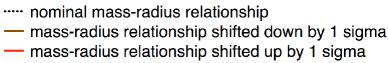
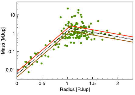
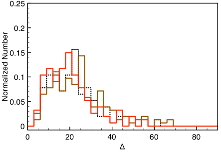
Figure 1.— (Top) Observed transiting exoplanets with known masses and radii shown in green, and the corresponding mass-radius relationship. (Bottom) Dependence of the observed dynamical spacing distribution on the choice of mass-radius relationship. In both panels, the nominal mass-radius relationship as defined in Equations (3) and (4) is shown in black, and the mass-radius relationship shifted by one sigma to lower (higher) masses is shown in brown (red). $\Delta$ represents the number of mutual Hill radii between adjacent planets in multi-planet systems and is defined in Equation (5).

For orbital eccentricities, we adopted circular orbits, as we did in Fang & Margot (2012a). Eccentricities do not directly affect our calculation of dynamical spacing, as we will define below in Equation (5).

Regarding the multiplicity distribution in our model populations, we used a bounded uniform distribution with $\lambda=1.5-3.5$ with increments of 0.25 to assign the number of planets per system. A bounded uniform distribution has a single parameter $\lambda$ and is defined as follows: first, draw a value $N_{\rm max}$ (maximum number of planets) from a Poisson distribution with parameter $\lambda$ that ignores zero values, and second, draw the number of planets from a discrete uniform distribution with range $1-N_{\rm max}$ (Fang & Margot, 2012a). Thus, each planetary system will have at least one planet. For the inclination distribution of planetary orbits, we used a Rayleigh distribution with $\sigma=1,2^{\circ}$ as well as a Rayleigh of Rayleigh distribution with $\sigma_{\sigma}=1,2^{\circ}$. A Rayleigh of Rayleigh distribution has a single parameter $\sigma_{\sigma}$ and is defined as follows: first, draw a value $\sigma$ from a Rayleigh distribution with parameter $\sigma_{\sigma}$, and second, draw a value for inclination from a Rayleigh distribution with parameter $\sigma$ (Lissauer et al., 2011b). These specific multiplicity and inclination distributions were chosen because they yielded fits consistent with transit numbers and transit duration ratios from Kepler detections (see Fang & Margot, 2012a). Combinations of these specific multiplicity and inclination distributions add up to a total of 36 possibilities.

The difference between model populations generated in Fang & Margot (2012a) and the model populations generated in this study is the treatment of planetary separations, since here we wish to determine the underlying dynamical spacing of planetary systems. We used a separation criterion $\Delta$ to assess the dynamical spacing between all adjacent planets in multi-planet systems, where $\Delta$ is defined as (e.g., Gladman, 1993; Chambers et al., 1996)

$$\Delta=\frac{a_{2}-a_{1}}{R_{H1,2}},$$ (5)

with

$$R_{H1,2}=\left(\frac{M_{1}+M_{2}}{3M_{*}}\right)^{1/3}\frac{a_{1}+a_{2}}{2}.$$ (6)

In these equations, $a$ is the semi-major axis, $R_{H1,2}$ is the mutual Hill radius, and $M$ is the mass. Subscripts $*$, $1$, and $2$ refer to the star, the inner planet, and the outer planet, respectively. For a two-planet system not in resonance, the planets are required to be spaced with $\Delta\gtrsim 3.46$ in order to be Hill stable.

In our model populations, adjacent planets in multi-planet systems were spaced according to a prescribed $\Delta$ distribution. We used a shifted Rayleigh distribution, which is the same as a regular Rayleigh distribution except shifted to the right by 3.5 (since we require this distribution to provide values of $\Delta$ that meet the minimum Hill stability limit). Such a distribution, as we will show, matches the observed sample well. The mathematical form of a shifted Rayleigh distribution $f$ is

$$f(\Delta)=\dfrac{\Delta-3.5}{\sigma^{2}}e^{-(\Delta-3.5)^{2}/(2\sigma^{2})},$$ (7)

and is described by a single parameter $\sigma$. In our model populations, we explored values of $\sigma=$10$-$20 with increments of 0.5 for a total of 21 possibilities. We chose this range of $\sigma$ values based on the location of the observed $\Delta$ distribution (blue histogram in Figure 2) with its approximate peak at about 20 mutual Hill radii. This chosen range of $\sigma$ values allowed us to explore different distributions of dynamical spacing that spanned a reasonable range of possible model $\Delta$ distributions. Increments of 0.5 were chosen as a trade-off between resolution and computational limitations. As will be seen in Section 2.2, the statistically good match between the data and the best-fit model demonstrates that our increments are sufficiently small and have appropriately sampled the possible range of $\Delta$ distributions.

In order to enforce that adjacent planets are spaced according to the prescribed $\Delta$ distribution, we performed the following steps. For each synthetic planetary system, the first planet’s orbital period is drawn from the debiased period distribution. If the system’s multiplicity is greater than one, for the second planet we draw its separation $\Delta$ from the first planet using the prescribed $\Delta$ distribution and we also draw a value from the debiased period distribution. If that value is less/greater than the first planet’s period, then the second planet will be the inner/outer planet and its exact period will be calculated by satisfying the drawn $\Delta$ separation from the first planet. This process repeats if the system has additional planets. These steps are different from Fang & Margot (2012a), where in that study all planetary orbital periods were chosen by drawing them from a debiased distribution. We verified that the periods drawn to match the $\Delta$ distribution provide a very close match to the debiased period distribution as well.

After the creation of each model population, we performed synthetic observations of each population’s planetary systems by the Kepler spacecraft in order to determine which planets were transiting and detectable (see Fang & Margot, 2012a). The transiting requirement was evaluated by picking a random line-of-sight (i.e., picking a random point on the celestial sphere) and computing the planet$-$star distance projected on the plane of the sky. The minimum of that distance was compared to the radius of the host star to determine if the planet in our simulations transited or not. The detection requirement was assessed by calculating each transiting planet’s SNR, defined as

$${\rm SNR}=\left(\dfrac{R}{R_{*}}\right)^{2}\dfrac{\sqrt{N}}{\sigma_{*}},$$ (8)

where the first fraction gives the depth of the transit, $N$ represents the number of transits up to Quarter 6, and $\sigma_{*}$ represents stellar noise (Combined Differential Photometric Precision or CDPP; Christiansen et al., 2012). Since CDPP is quarter-to-quarter dependent, we used the median CDPP value over all available quarters. In the calculation of SNR, we took into account gaps between Kepler quarters, the fact that not all stars are observed each quarter, and a 95% duty cycle (Fang & Margot, 2012a). If the calculated SNR for a transiting planet met or exceeded the SNR threshold for detection (SNR=10), then it was considered detectable.

Lastly, we determined the goodness-of-fit between each model population’s detected planets and the actual Kepler detections. This was ascertained by comparing the $\Delta$ distributions of adjacent planets in their multi-planet systems. We performed a Kolmogorov-Smirnov (K-S) test to assess the fit between the $\Delta$ distributions, and this comparison yielded a p-value that we used to evaluate the null hypothesis that the distributions emanate from the same parent distribution. This K-S probability was used to determine how well a particular model matched the observations. We also calculated the goodness-of-fit for multiplicity (by comparing with observed Kepler numbers of transiting systems using a chi-square test) and for inclination (by comparing with observed, normalized transit duration ratios using a K-S test) to check that they were consistent with the data (see Fang & Margot, 2012a). While we only generated model populations with underlying multiplicity and inclination distributions that are considered to be good fits to the data based on our previous work, this extra step allowed us to confirm that any models with acceptable $\Delta$ fits also produced acceptable multiplicity and inclination fits to the Kepler data. We determined which model populations were most consistent with the data by combining (multiplying) the probabilities associated with each one of the 3 statistical tests that probed multiplicity, inclination, and dynamical spacing. We assumed that these probabilities are independent.

Accounting for all combinations of multiplicity, inclination, and dynamical spacing distributions, in total we created 756 model populations with about 10⁶ planets each. As described earlier, each of these model populations underwent synthetic observations by Kepler as well as statistical tests. The next section presents our results.

2.2. Results

We report our results on the dynamical spacing (represented by the criterion $\Delta$) in multi-planet systems based on Kepler data. Using the methods described in the previous section, we determine that our best-fit model for the intrinsic $\Delta$ distribution is a shifted Rayleigh distribution (see Equation (7)) with $\sigma=14.5$.

This best-fit distribution is plotted in Figure 2, where we show its probability density distribution (top panel) as well as its cumulative probability distribution (bottom panel). This best-fit distribution has a mean value of $\Delta=21.7$ with a standard deviation of 9.5. About 50% of neighboring planet pairs have $\Delta$ separations larger than 20, and about 90% of neighboring planet pairs have $\Delta$ separations larger than 10. This best-fit distribution was obtained by considering shifted Rayleigh distributions with increments in $\sigma$ of 0.5. The mean values for distributions with $\sigma=14.0$ and $\sigma=15.0$ are $\Delta=22.3$ and $\Delta=21.0$, respectively. The combined probabilities for the match to the data using distributions with $\sigma=14.0$ and $\sigma=15.0$ are less than half the combined probability using $\sigma=14.5$.

Our results are valid for the range of stellar and planetary parameters given in Equations (1) and (2), most notably a minimum planet radius of 1.5 $R_{\earth}$ and a maximum orbital period of 200 days. It is possible that planets are actually even more closely spaced than this best-fit distribution if there are planets located in intermediate locations with radii less than 1.5 $R_{\earth}$. Therefore, our findings about the $\Delta$ distribution can be used to represent the spacing of planetary systems confined to the scope of our study, or can serve as an upper limit for the spacing of planetary systems that include planets with smaller radii.

Figure 3 shows the comparison between the $\Delta$ distribution of simulated detections from this best-fit model’s population and the observed $\Delta$ from actual Kepler detections. Note that this figure does not show the underlying $\Delta$ distribution that is plotted in Figure 2; instead, this figure shows the distribution of simulated planets that would have been detected, in order to make an appropriate comparison with the observed $\Delta$ distribution. The K-S test for comparing these two distributions yields a p-value of 56%, indicating that we cannot reject the null hypothesis that these distributions are drawn from the same parent distribution. In other words, this model is consistent with the observations.

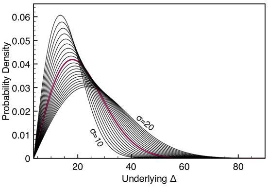
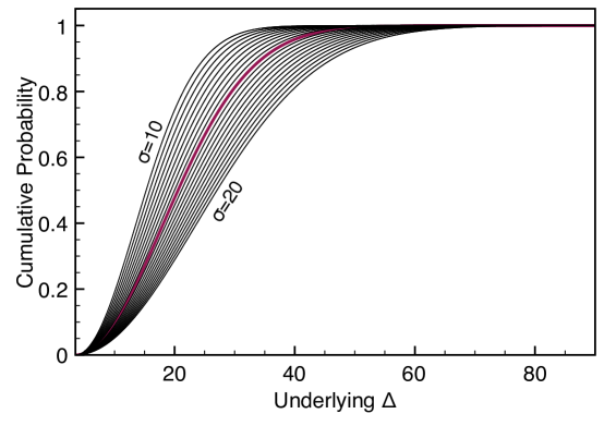
Figure 2.— The best-fit model’s underlying $\Delta$ distribution is shown as a magenta-colored curve. This distribution represents our best estimate of the true or intrinsic (i.e., free of observational bias) distribution of dynamical spacing between all neighboring planets meeting our orbital period and planet radius criteria. Recall that $\Delta$ represents the difference in semi-major axes between two adjacent orbits; it is expressed in units of the mutual Hill radius. The best-fit model is a shifted Rayleigh distribution as defined in Equation (7) with $\sigma=14.5$; the top plot depicts the probability density and the bottom plot shows the cumulative probability. The black-colored curves show the range and sampling frequency of model distributions that follow different $\sigma$ parameter values ranging from $\sigma=10$ to $\sigma=20$ with increments of 0.5, as examined in this study.

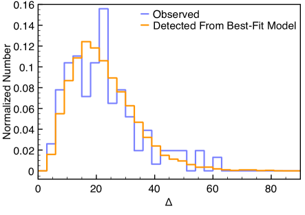
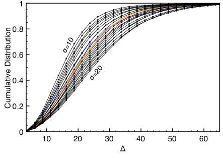
Figure 3.— The top plot shows the comparison between the observed $\Delta$ distribution from actual Kepler detections (shown in blue) and the $\Delta$ distribution from simulated detections in our best-fit model population (shown in orange); the K-S probability for this match is 56%. The bottom plot shows this comparison in cumulative form and its histogram points are connected by lines for easy viewing, and also shows the comparison with the properties of detected planets from other model populations ($\sigma=$10 to $\sigma=$20 with increments of 0.5; shown in black). The 99.5% confidence region of acceptable fits includes model populations with $\sigma$ ranging from 12.5 to 17.0.

Comparison between Figures 2 and 3 shows that the underlying $\Delta$ distribution is similar to the observed $\Delta$ distribution–both distributions have peaks near $\Delta$ $\sim$ 20. This suggests that the observed $\Delta$ distribution is not indicative of a significant population of non-transiting and/or low-SNR planets (within the planet radius and orbital period limits of our study) located in-between detected planets; otherwise, the underlying $\Delta$ distribution would have on average lower $\Delta$ values than those of the observed distribution. We caution again that our study cannot rule out the existence of a population of planets with $R<1.5R_{\earth}$, so the actual underlying $\Delta$ distribution could be different from what our results indicate. The similarity between the observed and underlying $\Delta$ distributions is due to the rarity of cases where a system has $\Delta_{\rm observed}>\Delta_{\rm underlying}$ (i.e., an undetected planet located in-between two detected planets). The stringent geometric probability of transit means that outer planets are more easily missed than inner planets. As a result, it will be rare to find cases where an intermediate planet is non-transiting and therefore missed, but both the innermost and outermost planets are transiting and detected. For such a case, which rarely occurs, the observed $\Delta$ would be greater than the underlying $\Delta$.

We discuss how we expect these results to change if an alternate mass-radius relationship is used. In particular, Figure 1 shows how the observed dynamical spacing distribution changes depending on various choices for the mass-radius relationship. For computational expediency, we chose to evaluate the effects of the mass-radius relationship on the observed $\Delta$ distribution. We use this as an approximation for the effects on the underlying $\Delta$ distribution, with the justification that the observed and underlying $\Delta$ distributions appear similar (see previous paragraph). For the mass-radius relationship shifted down by 1 sigma, the best-fitting shifted Rayleigh distribution has $\sigma$ = 16.5. For the mass-radius relationship shifted up by 1 sigma, the best-fitting shifted Rayleigh distribution has $\sigma$ = 12.5. As a result, we estimate that our derived dynamical spacing distribution can span $\sigma=$12.5$-$16.5 due to uncertainties in the mass-radius scaling.

3. Comparison to the Solar System, Kepler-11, and Kepler-36

We can compare our results (i.e., the intrinsic dynamical spacing or $\Delta$ distribution) with the dynamical spacing distribution of the Solar System, if we extrapolate beyond the radius and period limits (Equation (2)) of our study. Figure 4 shows our intrinsic $\Delta$ distribution of planetary systems overplotted with a histogram of the $\Delta$ distribution of the Solar System planets. From this figure, it is interesting to note that the distributions appear to be relatively similar and that the Solar System planets may be similarly spaced as most exoplanets in general. A K-S test between our cumulative $\Delta$ distribution and the sample of $\Delta$ values between adjacent planets in the Solar System yields a p-value of 66.2%, indicating that the Solar System $\Delta$ distribution is consistent with that of Figure 2.

The orbital evolution of the planets in the Solar System is known to be chaotic and unstable (e.g., Sussman & Wisdom, 1988; Laskar, 1989, 1990; Sussman & Wisdom, 1992; Laskar, 1994; Michtchenko & Ferraz-Mello, 2001; Lecar et al., 2001). The inner Solar System can be potentially unstable within the Sun’s remaining lifetime due to a secular resonance (Batygin & Laughlin, 2008). Laskar (1994) and Laskar & Gastineau (2009) have shown that inner planets could be ejected or collide. Numerical simulations of the planets in the outer Solar System suggest that they are packed (Barnes & Quinn, 2004; Raymond & Barnes, 2005; Barnes et al., 2008). All of these results suggest that the Solar System is dynamically packed. If we consider the Solar System to be dynamically packed then it is possible that other planetary systems with similar planet multiplicities and $\Delta$ distributions are also dynamically packed. This prompted us to verify whether planetary systems in general are dynamically packed (see Section 4).

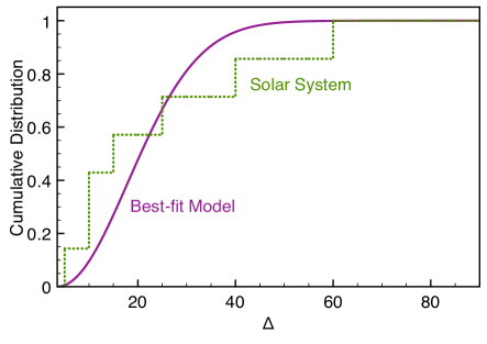
Figure 4.— Comparison of the cumulative $\Delta$ distribution between the best-fit model’s $\Delta$ distribution (i.e., shifted Rayleigh distribution with $\sigma=14.5$; purple solid line) and the Solar System’s $\Delta$ distribution (i.e., histogram based on its 8 planets; dotted green line).

Kepler-11 is a planetary system with six known transiting planets in a closely spaced configuration (Lissauer et al., 2011a). All six transiting planets have orbits smaller than the orbit of Venus, and five of the six transiting planets have orbits smaller than the orbit of Mercury. This appears to be a very compact system, and we calculate the $\Delta$ separations of the innermost five planets to be $\Delta_{\rm b-c}=$5.7, $\Delta_{\rm c-d}=$14.6, $\Delta_{\rm d-e}=$8.0, and $\Delta_{\rm e-f}=$11.2. We did not calculate the $\Delta$ separation of the f$-$g planet pair because the mass of planet g is not known and only has an upper limit. Accounting for the 1$\sigma$ uncertainties on mass reported by Lissauer et al. (2011a), the dynamical spacing of these pairs have the following ranges: $\Delta_{\rm b-c}=$5.1$-$7.0, $\Delta_{\rm c-d}=$13.0$-$17.3, $\Delta_{\rm d-e}=$7.2$-$8.8, and $\Delta_{\rm e-f}=$10.0$-$12.6. All of the Kepler-11 planets are within the planet radius and orbital period scope of our study, and we apply our knowledge of the intrinsic dynamical spacing (i.e., Figure 2) to this system. We find that the separation $\Delta_{\rm b-c}=$5.7 is more closely spaced than 98.9% of adjacent planet pairs in multi-planet systems, $\Delta_{\rm c-d}=$14.6 is more closely spaced than 74.6%, $\Delta_{\rm d-e}=$8.0 is more closely spaced than 95.3%, and $\Delta_{\rm e-f}=$11.2 is more closely spaced than 86.8%. These high percentages indicate that the planetary separations in the Kepler-11 system are much smaller than average separations in planetary systems, and we conclude that Kepler-11 is unusual in terms of the density of its configuration.

Kepler-36 has two known transiting planets with a large density contrast (their densities differ by a factor of $\sim$8) yet they orbit closely to one another (semi-major axes differ by $\sim$10%) (Carter et al., 2012). Such close orbits with dissimilar densities are unusual compared to the planets in the Solar System, where the denser terrestrial planets are located in the inner region and the less-dense giant planets are located in the outer region. We calculate the dynamical spacing between the two planets in Kepler-36 to be $\Delta$=4.7. In comparison to our intrinsic $\Delta$ distribution of dynamical spacing, a separation of $\Delta$=4.7 is more closely spaced than 99.7% of neighboring planet pairs of planetary systems in general.

4. Dynamical Packedness of Planets

Section 2.2 described the best-fit $\Delta$ distribution of planetary systems based on Kepler data, with a mean value of $\Delta=21.7$ (Figure 2). In this section, we investigate whether this distribution of $\Delta$ implies that planetary systems are dynamically packed or not. By dynamically packed, we refer to a planetary system that is filled to capacity and cannot include an additional planet without leading to instability.

To investigate whether planetary systems are dynamically packed, we performed long-term N-body integrations of planetary systems generated for our best-fit model population (see Sections 2.1-2.2). For each multiplicity (i.e., 2-planet systems, 3-planet systems, 4-planet systems), we randomly chose 1000 planetary systems for which we performed long-term integrations. In total, we performed 3000 integrations. We did not include single planet systems because they are irrelevant for studies of dynamical packedness and we did not include systems with multiplicities higher than 4 planets because they are relatively rare for our parameter space (Fang & Margot, 2012a).

For each integration, we added an additional planet when testing for stability; this planet had a mass equal to the lowest mass of all original planets and its initial conditions included an orbital eccentricity of zero, an inclination drawn from a Rayleigh of Rayleigh distribution with $\sigma_{\sigma}=1^{\circ}$ (see Section 2.1), and random values for its argument of pericenter, longitude of the ascending node, and mean anomaly. This additional planet was placed in-between the orbits of existing planets, and if there were 3 or 4 original planets, we randomly determined which 2 adjacent planets would be receiving a new neighbor. The additional planet’s semi-major axis was calculated so that it was located with equal mutual Hill radii distances between its neighboring planets. These initial conditions for the additional planet (e.g., low eccentricities, low inclinations, a mass equal to the lowest mass of original planets, a semi-major axis located at equal $\Delta$ distances from neighboring planets) are very conservative in the sense that we have chosen initial conditions that are very amenable to stability, as we determine whether a planetary system with this additional planet can remain stable or not.

Our simulations were performed using a hybrid symplectic/Bulirsch-Stoer integrator from the Mercury package (Chambers, 1999), and we used a timestep that covered 1/25 of the innermost planet’s orbital period. Simulations were performed for a length of 10⁸ years; the instability timescales had median values less than 10⁵ years. Possible outcomes included either a stable system with no instabilities or a system with at least one instability defined as a collision between the star and a planet, a collision between planets, and/or an ejected planet. All of these planetary systems were verified to be stable for 10⁸ years before adding the additional planet.

The results of our simulations can be divided into two camps. The first group is composed of planetary systems that became unstable in our integrations. This suggests that these planetary systems are dynamically packed, since the addition of another planet in an intermediate orbit resulted in an unstable planetary system. We found that 31%, 35%, and 45% of 2-, 3-, and 4-planet systems were unstable, respectively (Table 1). The second group is composed of planetary systems that did not exhibit any signs of instability. For these systems, although they were stable within the scope of our integrations, they may still be dynamically packed. Possible reasons include: an instability may occur on a longer timescale than our integration time, there may be additional planets in the system beyond the scope of our orbital period range of 200 days, or there may be additional planets in the system smaller than 1.5 $R_{\earth}$, which is the minimum radius of our study. All of these factors would affect the determination of the stability of the system, and so for this second group of systems we are agnostic about their dynamical packedness.

Accordingly, we can only confidently provide a lower limit on packed systems by concluding that at least 31$-$45% (depending on the system’s multiplicity) of planetary systems with dynamical spacings consistent with our best-fit $\Delta$ distribution (Figure 2) are dynamically packed. These lower limits are also presented in Table 1. Note that systems with lower multiplicity are more common (Fang & Margot, 2012a).

Table 1Lower Limits on the Percentage of Dynamically Packed Systems

System Multiplicity	Percentage of Packed Systems
2-Planet Systems	$\geq$ 31%
3-Planet Systems	$\geq$ 35%
4-Planet Systems	$\geq$ 45%

The packed planetary systems (PPS) hypothesis is the idea that all planetary systems are dynamically packed, and therefore cannot hold additional planets without becoming unstable. The results of our long-term numerical integrations are consistent with the PPS hypothesis, as we find a sizeable lower limit of 31$-$45% (depending on the system’s multiplicity) of planetary systems to be dynamically packed.

5. Conclusions

We have generated model populations of planetary systems and simulated observations of them by the Kepler spacecraft. By comparing the properties of detected planets in our simulations with the actual Kepler planet detections, we have determined the best-fit distribution of dynamical spacing between neighboring planets. This best-fit distribution is our best estimate of the underlying (i.e., free of observational bias) distribution of dynamical spacing for our orbital period ($P$ $\leq$ 200 days) and planet radius ($1.5~{}R_{\earth}\leq R\leq 30~{}R_{\earth}$) parameter regime. Stemming from this distribution, the main results of this study are:

1. On average, neighboring planets are spaced 21.7 mutual Hill radii apart, with a standard deviation of 9.5. This distance represents the typical dynamical spacing of neighboring planets for all systems included in the parameter space described above.

2. Our best-fit distribution of dynamical spacing is consistent with the dynamical spacing of neighboring planets in the Solar System, with a K-S p-value of 66.2%. If we consider the Solar System to be dynamically packed, then it is not unreasonable to ask whether other planetary systems with similar dynamical spacing are also dynamically packed.

3. Based on our best-fit distribution of planetary spacing: $\geq$31% of 2-planet systems, $\geq$35% of 3-planet systems, and $\geq$45% of 4-planet systems are dynamically packed. This means that such systems are filled to capacity and cannot hold another planet in an intermediate orbit without becoming unstable.

4. Our results on the dynamical packedness of planetary systems are consistent with the packed planetary systems hypothesis that all planetary systems are filled to capacity, as we find sizeable lower limits on the fraction of systems that are dynamically packed.

5. Compact systems such as Kepler-11 and Kepler-36 represent extremes in the dynamical spacing distribution. For example, the two known planets in Kepler-36 are more closely spaced than 99.7% of all neighboring planets represented by our orbital period and planet radius regime.

References

- Barnes et al. (2008) Barnes, R., Goździewski, K., & Raymond, S. N. 2008, ApJ, 680, L57
- Barnes & Greenberg (2007) Barnes, R. & Greenberg, R. 2007, ApJ, 665, L67
- Barnes & Quinn (2004) Barnes, R. & Quinn, T. 2004, ApJ, 611, 494
- Batalha et al. (2012) Batalha, N. M., Rowe, J. F., Bryson, S. T., Barclay, T., Burke, C. J., Caldwell, D. A., Christiansen, J. L., Mullally, F., Thompson, S. E., Brown, T. M., Dupree, A. K., Fabrycky, D. C., Ford, E. B., Fortney, J. J., Gilliland, R. L., Isaacson, H., Latham, D. W., Marcy, G. W., Quinn, S., Ragozzine, D., Shporer, A., Borucki, W. J., Ciardi, D. R., Gautier, III, T. N., Haas, M. R., Jenkins, J. M., Koch, D. G., Lissauer, J. J., Rapin, W., Basri, G. S., Boss, A. P., Buchhave, L. A., Charbonneau, D., Christensen-Dalsgaard, J., Clarke, B. D., Cochran, W. D., Demory, B.-O., Devore, E., Esquerdo, G. A., Everett, M., Fressin, F., Geary, J. C., Girouard, F. R., Gould, A., Hall, J. R., Holman, M. J., Howard, A. W., Howell, S. B., Ibrahim, K. A., Kinemuchi, K., Kjeldsen, H., Klaus, T. C., Li, J., Lucas, P. W., Morris, R. L., Prsa, A., Quintana, E., Sanderfer, D. T., Sasselov, D., Seader, S. E., Smith, J. C., Steffen, J. H., Still, M., Stumpe, M. C., Tarter, J. C., Tenenbaum, P., Torres, G., Twicken, J. D., Uddin, K., Van Cleve, J., Walkowicz, L., & Welsh, W. F. 2012, ArXiv e-prints
- Batygin & Laughlin (2008) Batygin, K. & Laughlin, G. 2008, ApJ, 683, 1207
- Carter et al. (2012) Carter, J. A., Agol, E., Chaplin, W. J., Basu, S., Bedding, T. R., Buchhave, L. A., Christensen-Dalsgaard, J., Deck, K. M., Elsworth, Y., Fabrycky, D. C., Ford, E. B., Fortney, J. J., Hale, S. J., Handberg, R., Hekker, S., Holman, M. J., Huber, D., Karoff, C., Kawaler, S. D., Kjeldsen, H., Lissauer, J. J., Lopez, E. D., Lund, M. N., Lundkvist, M., Metcalfe, T. S., Miglio, A., Rogers, L. A., Stello, D., Borucki, W. J., Bryson, S., Christiansen, J. L., Cochran, W. D., Geary, J. C., Gilliland, R. L., Haas, M. R., Hall, J., Howard, A. W., Jenkins, J. M., Klaus, T., Koch, D. G., Latham, D. W., MacQueen, P. J., Sasselov, D., Steffen, J. H., Twicken, J. D., & Winn, J. N. 2012, Science, 337, 556
- Chambers (1999) Chambers, J. E. 1999, MNRAS, 304, 793
- Chambers et al. (1996) Chambers, J. E., Wetherill, G. W., & Boss, A. P. 1996, Icarus, 119, 261
- Christiansen et al. (2012) Christiansen, J. L., Jenkins, J. M., Caldwell, D. A., Burke, C. J., Tenenbaum, P., Seader, S., Thompson, S. E., Barclay, T. S., Clarke, B. D., Li, J., Smith, J. C., Stumpe, M. C., Twicken, J. D., & Van Cleve, J. 2012, PASP, 124, 1279
- Fang & Margot (2012a) Fang, J. & Margot, J.-L. 2012a, ArXiv e-prints
- Fang & Margot (2012b) —. 2012b, ApJ, 751, 23
- Gladman (1993) Gladman, B. 1993, Icarus, 106, 247
- Howard et al. (2012) Howard, A. W., Marcy, G. W., Bryson, S. T., Jenkins, J. M., Rowe, J. F., Batalha, N. M., Borucki, W. J., Koch, D. G., Dunham, E. W., Gautier, T. N., Cleve, J. V., Cochran, W. D., Latham, D. W., Lissauer, J. J., Torres, G., Brown, T. M., Gilliland, R. L., Buchhave, L. A., Caldwell, D. A., Christensen-Dalsgaard, J., Ciardi, D., Fressin, F., Haas, M. R., Howell, S. B., Kjeldsen, H., Seager, S., Rogers, L., Sasselov, D. D., Steffen, J. H., Basri, G. S., Charbonneau, D., Christiansen, J., Clarke, B., Dupree, A., Fabrycky, D. C., Fischer, D. A., Ford, E. B., Fortney, J. J., Tarter, J., Girouard, F. R., Holman, M. J., Johnson, J. A., Klaus, T. C., Machalek, P., Moorhead, A. V., Morehead, R. C., Ragozzine, D., Tenenbaum, P., Twicken, J. D., Quinn, S. N., Isaacson, H., Shporer, A., Lucas, P. W., Walkowicz, L. M., Welsh, W. F., Boss, A., Devore, E., Gould, A., Smith, J. C., Morris, R. L., Prsa, A., Morton, T. D., Still, M., Thompson, S. E., Mullally, F., Endl, M., & MacQueen, P. J. 2012, The Astrophysical Journal Supplement Series, 201, 15
- Ji et al. (2005) Ji, J., Liu, L., Kinoshita, H., & Li, G. 2005, ApJ, 631, 1191
- Laskar (1989) Laskar, J. 1989, Nature, 338, 237
- Laskar (1990) —. 1990, Icarus, 88, 266
- Laskar (1994) —. 1994, A&A, 287, L9
- Laskar & Gastineau (2009) Laskar, J. & Gastineau, M. 2009, Nature, 459, 817
- Lecar et al. (2001) Lecar, M., Franklin, F. A., Holman, M. J., & Murray, N. J. 2001, ARA&A, 39, 581
- Lissauer et al. (2011a) Lissauer, J. J., Fabrycky, D. C., Ford, E. B., Borucki, W. J., Fressin, F., Marcy, G. W., Orosz, J. A., Rowe, J. F., Torres, G., Welsh, W. F., Batalha, N. M., Bryson, S. T., Buchhave, L. A., Caldwell, D. A., Carter, J. A., Charbonneau, D., Christiansen, J. L., Cochran, W. D., Desert, J.-M., Dunham, E. W., Fanelli, M. N., Fortney, J. J., Gautier, III, T. N., Geary, J. C., Gilliland, R. L., Haas, M. R., Hall, J. R., Holman, M. J., Koch, D. G., Latham, D. W., Lopez, E., McCauliff, S., Miller, N., Morehead, R. C., Quintana, E. V., Ragozzine, D., Sasselov, D., Short, D. R., & Steffen, J. H. 2011a, Nature, 470, 53
- Lissauer et al. (2011b) Lissauer, J. J., Ragozzine, D., Fabrycky, D. C., Steffen, J. H., Ford, E. B., Jenkins, J. M., Shporer, A., Holman, M. J., Rowe, J. F., Quintana, E. V., Batalha, N. M., Borucki, W. J., Bryson, S. T., Caldwell, D. A., Carter, J. A., Ciardi, D., Dunham, E. W., Fortney, J. J., Gautier, III, T. N., Howell, S. B., Koch, D. G., Latham, D. W., Marcy, G. W., Morehead, R. C., & Sasselov, D. 2011b, ApJS, 197, 8
- Menou & Tabachnik (2003) Menou, K. & Tabachnik, S. 2003, ApJ, 583, 473
- Michtchenko & Ferraz-Mello (2001) Michtchenko, T. A. & Ferraz-Mello, S. 2001, AJ, 122, 474
- Ragozzine et al. (2012) Ragozzine, D. et al. 2012, in AAS/Division for Planetary Sciences Meeting Abstracts, Vol. 44, AAS/Division for Planetary Sciences Meeting Abstracts
- Raymond & Barnes (2005) Raymond, S. N. & Barnes, R. 2005, ApJ, 619, 549
- Raymond et al. (2008) Raymond, S. N., Barnes, R., & Gorelick, N. 2008, ApJ, 689, 478
- Raymond et al. (2006) Raymond, S. N., Barnes, R., & Kaib, N. A. 2006, ApJ, 644, 1223
- Rivera & Haghighipour (2007) Rivera, E. & Haghighipour, N. 2007, MNRAS, 374, 599
- Sussman & Wisdom (1988) Sussman, G. J. & Wisdom, J. 1988, Science, 241, 433
- Sussman & Wisdom (1992) —. 1992, Science, 257, 56
- Youdin (2011) Youdin, A. N. 2011, ApJ, 742, 38