Dynamical localization of chaotic eigenstates in the mixed-type systems: spectral statistics in a billiard system after separation of regular and chaotic eigenstates

Abstract

We study the quantum mechanics of a billiard (Robnik 1983) in the regime of mixed-type classical phase space (the shape parameter $\lambda=0.15$) at very high-lying eigenstates, starting at about 1.000.000th eigenstate and including the consecutive 587654 eigenstates. By calculating the normalized Poincaré Husimi functions of the eigenstates and comparing them with the classical phase space structure, we introduce the overlap criterion which enables us to separate with great accuracy and reliability the regular and chaotic eigenstates, and the corresponding energies. The chaotic eigenstates appear all to be dynamically localized, meaning that they do not occupy uniformly the entire available chaotic classical phase space component, but are localized on a proper subset. We find with unprecedented precision and statistical significance that the level spacing distribution of the regular levels obeys the Poisson statistics, and the chaotic ones obey the Brody statistics, as anticipated in a recent paper by Batistić and Robnik (2010), where the entire spectrum was found to obey the BRB statistics. There are no effects of dynamical tunneling in this regime, due to the high energies, as they decay exponentially with the inverse effective Planck constant which is proportional to the square root of the energy.

Benjamin.Batistic@gmail.com, Robnik@uni-mb.si

1 Introduction

In quantum chaos [1, 2, 3] of general (generic) time-independent (autonomous) Hamilton systems in the strict semiclassical limit we can conceptually separate regular and chaotic eigenstates. This picture goes back to the work by Percival in 1973 [4] and Berry and Robnik in 1984 [5]. One of the main results in quantum chaos is the fact that in classically fully chaotic (ergodic, autonomous Hamilton) systems with the purely discrete spectrum the fluctuations of the energy spectrum around its mean behaviour obey the statistical laws described by the Gaussian Random Matrix Theory (RMT) [6, 7], provided that we are in the sufficiently deep semiclassical limit. The latter condition means that all relevant classical transport times, like the typical ergodic time, or diffusion time, are smaller than the so-called Heisenberg time, or break time, given by $t_{H}=2\pi\hbar/\Delta E$, where $h=2\pi\hbar$ is the Planck constant and $\Delta E$ is the mean energy level spacing, such that the mean energy level density is $\rho(E)=1/\Delta E$. This statement is known as the Bohigas - Giannoni - Schmit (BGS) conjecture and goes back to their pioneering paper in 1984 [8], although some preliminary ideas were published in [9]. Since $\Delta E\propto\hbar^{d}$, where $d$ is the number of degrees of freedom (= the dimension of the configuration space), we see that for sufficiently small $\hbar$ the stated condition will always be satisfied. Alternatively, fixing the $\hbar$, we can go to high energies such that the classical transport times become smaller than $t_{H}$. The role of the antiunitary symmetries that classify the statistics in terms of GOE, GUE or GSE (ensembles of RMT) has been explained in [10], see also [11] and [1, 2, 3, 6]. The theoretical foundation for the BGS conjecture has been initiated first by Berry [12], using the Gutzwiller periodic orbit theory (trace formula) [13] (for an excellent exposition see [1]) and later further developed by Richter and Sieber [14], arriving finally in the almost-final proof proposed by the group of F. Haake [15, 16, 17, 18].

On the other hand, if the system is classically integrable, Poisson statistics applies, as is well known and goes back to the work by Berry and Tabor in 1977 (see [1, 2, 3] and the references therein, and for the recent advances [19]).

In the mixed-type regime, where classical regular regions coexist in the classical phase space with the chaotic regions, being a typical KAM-scenario which is the generic situation, the so-called Principle of Uniform Semiclassical Condensation (of the Wigner functions of the eigenstates; PUSC) applies, based on the ideas by Berry [20], and further extended by Robnik [3]. If the stated semiclassical condition is satisfied, the chaotic eigenstates are uniformly extended, and consequently the Berry-Robnik statistics [5, 21] is observed - see also [3]. If the semiclassical condition stated above requiring that $t_{H}$ is larger than all classical transport times is not satisfied, the chaotic eigenstates will not be extended but localized and the Berry-Robnik statistics must be generalized as explained in [22, 23, 3, 24, 25] and in this paper.

The relevant papers dealing with the mixed-type regime after the work [5] are [21] - [31] and the most recent advance was published in [24]. If the couplings between the regular eigenstates and chaotic eigenstates become important, due to the dynamical tunneling, we can use the ensembles of random matrices that capture these effects [32, 24]. As the tunneling strengths typically decrease exponentially with the inverse effective Planck constant, they rapidly disappear with increasing energy, or by decreasing the value of the Planck constant. In this work we shall deal only with high-lying eigenstates, and therefore we can neglect the effects of tunneling.

However, quite generally, if the semiclassical condition is not satisfied, such that $t_{H}$ is no longer larger than the relevant classical transport time, like e.g. the diffusion time in fully chaotic but slowly ergodic systems, we find the so-called dynamical localization, or Chirikov localization. Dynamical localization was discovered in time dependent systems [33]. It was intensely studied since then in particular by Chirikov, Casati, Izrailev, Shepelyanski and Guarneri, in the case of the kicked rotator as reviewed in [34]. See also the references [35]-[38], and the most recent work [39]. For a general overview of the time dependent Floquet systems see also [1, 2]. It has been observed that in parallel with the localization of the eigenstates one observes the fractional power law level repulsion (of the quasienergies) even in fully chaotic regime (of the finite dimensional kicked rotator), and it is believed that this picture applies also to time independent (autonomous) Hamilton systems and their eigenstates [39]. (See the excellent review of localization in time independent billiards by Prosen in [40].) Indeed, this has been analyzed with unprecedented precision and statistical significance recently by Batistić and Robnik [24] in case of mixed-type systems, and the present work is being extended in the analysis of separated regular and chaotic eigenstates. An early attempt of separation of eigenstates in the billiard system has been published in [41], using a different approach at much lower energies and with much smaller statistical significance. In [42] mushroom billiards were studied at much lower energies and with much smaller statistical significance, where the aspects of tunneling were investigated in the first place, but not the dynamical localization, although a clear deviation from the GOE statistics was found in the chaotic eigenstates.

In this paper we introduce a criterion for classifying eigenstates as regular and chaotic, and moreover, we show that the regular levels obey the Poisson statistics, whilst the chaotic dynamically localized eigenenergies obey exceedingly well the Brody distribution [43], with the Brody parameter values $\beta$ within the interval $[0,1]$, where $\beta=0$ yields the Poisson distribution in case of the strongest localization, and $\beta=1$ gives the Wigner surmise (2D GOE, as an excellent approximation of the infinite dimensional GOE), which describes the extended chaotic eigenstates. It turns out that the Brody distribution introduced in [43], see also [44], fits the empirical data much better than e.g. the distribution function proposed by F. Izrailev (see [35, 34] and the references therein).

It is well known that Brody distribution so far has no theoretical foundation, but our empirical results show that we have to consider it seriously in dynamically localized chaotic eigenstates, thereby being motivated for seeking its physical foundation, and an analogous result was obtained in the recent work of Manos and Robnik (2013) [39] in the analysis of the quantum kicked rotator, where the object of study are the eigenstates of the Floquet operator and the statistical properties of the spectrum of eigenphases (quasienergies) in classically fully chaotic regime.

In the Hamilton systems with classically mixed-type dynamics, which is the generic case, we have classically regular quasi-periodic motion on $d$-dim invariant tori ($d$ is the number of freedoms) for some initial conditions (with the fractional Liouville volume $\rho_{1}$) and chaotic motion for the complementary initial conditions (with the fractional Liouville volume $\rho_{2}=1-\rho_{1}$). The chaotic set might be further decomposed into several chaotic regions (invariant components) in case $d=2$, whilst for $d>2$ it is strictly speaking always just one chaotic set due to the Arnold diffusion on the Arnold web, which pervades the entire phase space. In sufficiently deep semiclassical limit the Berry-Robnik picture [5] is established, based on the statistically independent superposition of the regular (Poissonian) and chaotic level sequences, based on PUSC, as explained above.

In this paper we shall consider only the case of just one chaotic component, although the results can be easily generalized for more than one chaotic component. This picture gives an excellent approximation for the statistics of spectral fluctuations of the mixed-type systems, if the largest chaotic component is much larger than the next largest one, which typically indeed is the case e.g. in 2D billiards.

The energy spectrum of the mixed-type system with one regular and one chaotic component can be described in the Berry-Robnik (BR) regime of sufficiently small effective Planck constant $\hbar_{eff}$ by the following formula for the gap probability $E(S)$,

$$E(S)=E_{r}(\rho_{1}S)E_{c}(\rho_{2}S)$$ (1)

and the level spacing distribution $P(S)$ (see e.g. [3]) is of course always given as the second derivative of the gap probability, namely $P(S)=d^{2}E(S)/dS^{2}$, so that we have

$$P(S)=\frac{d^{2}}{dS^{2}}E_{r}(\rho_{1}S)E_{c}(\rho_{2}S)=\frac{d^{2}E_{r}}{dS^{2}}E_{c}+2\frac{dE_{r}}{dS}\frac{dE_{c}}{dS}+E_{r}\frac{d^{2}E_{c}}{dS^{2}}.$$ (2)

This factorization formula (1) is a direct consequence of the statistical independence, justified by PUSC. Here by $E_{r}(S)=\exp(-S)$ we denote the gap probability for the Poissonian sequence with the mean level density one. By $E_{c}(S)$ we denote the gap probability for the chaotic level sequence with the mean level density (and spacing) one. Note that the classical parameter $\rho_{1}$ and its complement $\rho_{2}=1-\rho_{1}$ enter the expression as weights in the arguments of the gap probabilities.

Using the Bohigas-Giannoni-Schmit conjecture we conclude that in the sufficiently deep semiclassical limit $E_{c}(S)$ is given by the RMT, and can be well approximated by the Wigner surmise

$$P_{W}(S)=\frac{\pi S}{2}\exp\left(-\frac{\pi S^{2}}{4}\right),\;\;F_{W}(S)=1-W_{W}(S)=\exp\left(-\frac{\pi S^{2}}{4}\right),$$ (3)

such that $E_{c}(S)$ is equal to

$$E_{W}(S)=1-{\rm erf}\left(\frac{\sqrt{\pi}S}{2}\right)={\rm erfc}\left(\frac{\sqrt{\pi}S}{2}\right),$$ (4)

where ${\rm erf}(x)=\frac{2}{\sqrt{\pi}}\int_{0}^{x}e^{-u^{2}}du$ is the error integral and ${\rm erfc}(x)$ its complement, i.e. ${\rm erfc}(x)=1-{\rm erf}(x)$. In the equation (3) $W_{W}(S)$ denotes the cumulative Wigner level spacing distribution $W_{W}(S)=\int_{0}^{S}P_{W}(x)\;dx$ and $F_{W}$ its complement. The explicit Berry-Robnik level spacing distribution (in the special case of one regular and one chaotic component) follows immediately,

$$P_{BR}(S)=e^{-\rho_{1}S}\left\{e^{-\frac{\pi\rho_{2}^{2}S^{2}}{4}}\left(2\rho_{1}\rho_{2}+\frac{\pi\rho_{2}^{3}S}{2}\right)+\rho_{1}^{2}{\rm erfc}\left(\frac{\sqrt{\pi}\rho_{2}S}{2}\right)\right\}.$$ (5)

The correctness of this distribution function in the BR regime (sufficiently small $\hbar_{eff}$) is by now very well established in highly accurate numerical calculations for all $E(k,L)$ probabilities, not only the gap probability [21].

In the present work the above basic BR formula (1) is generalized as in [24] to capture the dynamical localization effects, responsible for the deviation from the BR regime.

At not sufficiently small $\hbar_{eff}$ (e.g. in billiards this means at low energies) the chaotic eigenstates (their Wigner functions in the phase space) are not uniformly extended over the entire classically allowed chaotic component, but are dynamically localized. Thus we see the transition from GOE in case of extended chaotic states to the Poissonian statistics in case of strong localization. The level spacing distribution in such a transition regime of localized chaotic eigenstates can be described by the Brody distribution with the only one family parameter $\beta$,

$$P_{B}(S)=C_{1}S^{\beta}\exp\left(-C_{2}S^{\beta+1}\right),\;\;\;W_{B}(S)=1-\exp\left(-C_{2}S^{\beta+1}\right),$$ (6)

where the two parameters $C_{1}$ and $C_{2}$ are determined by the two normalizations $<1>=<S>=1$, and are given by

$$C_{1}=(\beta+1)C_{2},\;\;\;C_{2}=\left(\Gamma\left(\frac{\beta+2}{\beta+1}\right)\right)^{\beta+1}$$ (7)

with $\Gamma(x)$ being the Gamma function. As mentioned before, if we have extended chaotic states $\beta=1$ and RMT (3) applies, whilst in the strongly localized regime $\beta=0$ and we have Poissonian statistics. Again, by $W_{B}(S)$ we denote the cumulative Brody level spacing distribution, $W_{B}(S)=\int_{0}^{S}P_{B}(x)\;dx$. The corresponding gap probability is

$$E_{B}(S)=\frac{1}{(\beta+1)\Gamma\left(\frac{\beta+2}{\beta+1}\right)}Q\left(\frac{1}{\beta+1},\left(\Gamma\left(\frac{\beta+2}{\beta+1}\right)S\right)^{\beta+1}\right)$$ (8)

where $Q(\alpha,x)$ is the incomplete Gamma function

$$Q(\alpha,x)=\int_{x}^{\infty}t^{\alpha-1}e^{-t}dt.$$ (9)

By choosing $E_{c}(S)$ in equation (1) as given in (8) we are able to describe the localization effects on the chaotic component. Such approach has been already proposed in the paper by Prosen and Robnik in 1994 [22, 23] and the resulting level spacing distribution, emerging from this assumption, was called Berry-Robnik-Brody (BRB). It has two parameters, the classical parameter $\rho_{1}$ and the quantum parameter $\beta$. It will turn out that this description is indeed excellent, and has been verified to high accuracy by Batistić and Robnik [24].

The applicability of the Brody distribution in this context is theoretically still not well understood, but we shall see that the theory describes very well the empirical data from the highly accurate energy spectra of billiards at energies around and below the deep semiclassical (Berry-Robnik) regime. Therefore, the resulting theory is of semiempirical nature, but seems to be quasi-universal in the sense that below the Berry-Robnik regime we indeed find spectral fluctuations, in particular the level spacing distribution, which are well described by our theory on the very finest scale of level spacings. We have also tried to use other one-parametric level spacing distributions instead of Brody, in particular those proposed and studied in Izrailev’s papers [35, 38, 34] (see also [45]), but must definitely conclude that the Brody distribution is quite special, it gives by far the best agreement between the theory and real spectra. Izrailev’s intermediate level spacing distribution intended to capture the localization effects manifested in the quantal spectra is given by

$$P_{I}(S)=A\left(\frac{1}{2}\pi S\right)^{\beta}\exp\left[-\frac{1}{16}\beta\pi^{2}S^{2}-\left(B-\frac{1}{4}\pi\beta\right)S\right],$$ (10)

where the constants $A$ and $B$ are determined by the normalizations $<1>=<S>=1$.

As we shall show the dynamical localization effects can persist up to very high-lying eigenstates, even up to one million, whilst - as mentioned before - the tunneling effects occur usually only at very low-lying eigenstates, due to the exponential dependence on the reciprocal effective Planck constant, $\propto\exp(-const./\hbar_{eff})$, and thus can be neglected in our case.

The paper is structured as follows: In section 2 the billiard system is defined as introduced by Robnik [46, 47] with shape parameter $\lambda=0.15$, and we describe the Poincaré Husimi functions, in section 3 we introduce the method of classifying and separating regular and chaotic eigenstates in terms of normalized Poincaré Husimi functions (which are Gaussian-smoothed Wigner functions), in section 4 we present the results, and in section 5 we conclude and discuss the results.

2 Introducing the model system and the definition of the problem

As an interesting and frequently studied model system we have chosen the billiard introduced by Robnik in references [46]-[47], whose boundary is defined by the quadratic conformal map of the unit circle $|z|=1$ of the $z$-complex plane onto the $w$-complex plane (which is the physical plane) as follows

$$w=z+\lambda z^{2}.$$ (11)

The choice of this quadratic map has two reasons: (i) it allows for an elegant method [47] to solve the Helmholtz equation in the $w$-plane by transforming back to the $z$-plane, and (ii) it is the simplest one with nontrivial classical dynamics [46]. The shape parameter $\lambda$ goes from 0 (circle; integrability) to 1/2 (cardioid billiard; ergodicity: full chaos [48]). For $0\leq\lambda\leq 1/4$ the billiard boundary is convex and thus we observe the existence of Lazutkin’s caustics [49, 50] near the boundary in the configuration space, which are the projections of the KAM invariant tori (in the phase space). When increasing the value of $\lambda$ from 0 we have at $\lambda=1/4$ for the first time a point of zero curvature located at $z=-1$, and thus $w=-1+\lambda$. By a theorem due to J. Mather this is a sufficient condition for the destruction of Lazutkin’s caustics and of the underlying invariant tori near the boundary, which in turn is a necessary condition for the ergodicity of the classical billiard dynamics. However, at $\lambda\geq 1/4$ the dynamics is not yet ergodic, fully chaotic, as there are still some tiny KAM islands of stability [51], not so easy to detect numerically. Nevertheless, for $\lambda=1/2$, the ergodicity was proven rigorously by Markarian [48].

We are interested in the mixed-type case, within the interval $0<\lambda<1/4$, where the chaotic regions coexist with the regular regions in the phase space. In particular, we have chosen $\lambda=0.15$, which is one of the most frequently studied cases in [26, 27, 22, 23, 25, 52, 53, 41]. The fractional phase space volume $\rho_{1}$ of the classically regular part of the phase space (not to be confused with the area on the Poincaré surface of section!) is equal to $0.175$, as has been carefully studied in [52, 24]. In a previous work [22, 23] $\rho_{1}$ was estimated numerically as $\rho_{1}=0.36$, which is due to the technical difficulties in distinguishing the regular regions and slowly diffusing chaotic regions due to the sticky objects in the classical phase space. These difficulties were overcome in [52] and [24], using the new methods based on the ideas and approach in [54]. The estimate $\rho_{1}=0.175$ is now believed to be accurate within at least one percent relative error.

The classical mechanics of 2D billiards is studied in the Poincaré-Birkhoff coordinates $(s,p)$, where $s$ is the arclength parameter going from 0 to ${\cal L}$, the perimeter of the billiard domain, in our case counted anticlockwise from the point $w=1+\lambda$, and $p$ is simply the sine of the reflection angle, which goes from -1 to +1. The bounce map is defined by the free motion between the collision points on the boundary, obeying the specular reflection law upon each collision. Thus, the complete information on the classical dynamics is contained in the structure of the bounce map on the cylinder $(s,p)$. When analyzing the quantum mechanics of this system, we would like to find an analogous two dimensional space which also contains the complete information about the quantum mechanics, namely about the eigenfunctions. This is the space of the so-called Poincaré Husimi functions (see [55] and the references therein) that we introduce below.

The quantum mechanics of the billiard system comprises the study of the solution of the Helmholtz equation for the billiard domain ${\cal B}$,

$$\Delta\psi+k^{2}\psi=0,$$ (12)

with the Dirichlet boundary condition $\psi=0$ on the boundary $\partial{\cal B}$. We have used a number of methods, like in [24], to calculate the eigenenergies $E_{j}=k_{j}^{2}$, where $j$ is the counting index $j=1,2,3,\dots$, and the associated eigenfunctions are denoted by $\psi_{j}({\bf r})$.

Introducing the important quantity $u(s)$, the normal derivative of the eigenfunction $\psi$ on the boundary, from here onwards called boundary function,

$$u(s)={\bf n}\cdot\nabla_{{\bf r}}\psi\left({\bf r}(s)\right),$$ (13)

where ${\bf n}$ is the unit outward vector normal to the boundary at position $s$, we can show [56] that the eigenvalue problem (12) is equivalent to the following integral equation

$$u(s)=-2\oint dt\;u(t)\;{\bf n}\cdot\nabla_{{\bf r}}G({\bf r},{\bf r}(t)).$$ (14)

Here ${\bf r}(t)$ is the position vector at the point $s=t$ on the boundary, whilst ${\bf r}$ is the position vector inside the billiard ${\cal B}$. $G({\bf r},{\bf r}(t))$ is the free particle Green function, namely

$$G({\bf r},{\bf r^{\prime}})=-\frac{i}{4}H_{0}^{(1)}(k|{\bf r}-{\bf r^{\prime}}|),$$ (15)

where $H_{0}^{(1)}(x)$ is the zero order Hankel function of the first kind. It is important to know that knowing $u_{j}(s)$ for a certain eigenfunction $j$, we can immediately calculate the wave function $\psi_{j}({\bf r})$ within the interior of the billiard domain by

$$\psi_{j}({\bf r})=-\oint dt\;u_{j}(t)\;G\left({\bf r},{\bf r}(t)\right).$$ (16)

Thus, in certain analogy to the classical mechanics, the quantum mechanics is completely described by the boundary functions $u_{j}(s)$. Finally, there is the important identity [56]

$$\frac{1}{2}\oint dt\;{\bf n}(t)\cdot{\bf r}(t)\;u_{j}(t)^{2}=k_{j}^{2}.$$ (17)

The quantum analogy of the classical phase space is the space of Wigner functions [57] or of other phase space representations of quantum states in general. The Wigner functions are real but not positive definite functions, and exhibit lots of oscillations around the zero level also in the regime where the quantum probability density is low and thus such structures often obscure the main physical aspects of the phenomena. Nevertheless, they do uniformly condense on the classical invariant objects, according to the mentioned PUSC [3] in the introduction. There are different ways of defining positive definite phase space functions, but Husimi functions [58] are perhaps the best way to do it. They are in fact Gaussian smoothed Wigner functions. In general, we define them by the projection of the wave function onto a coherent state. One of the possible formulations can be found in [55], whose definitions and the notation we shall use in what follows. The idea and the approach (in slightly different form) goes back to the works [59], [60] and [61]. The most important idea is to define the one-dimensional coherent states onto which we project the boundary functions $u_{j}(s)$. For this reason, and due to the analogy with the classical dynamics and its Poincaré surface of section on the cylinder $(s,p)$, the underlying Husimi functions are called Poincaré Husimi functions [55].

The key idea is to introduce one-dimensional coherent state as a function of the coordinate $s$ on the boundary $\partial{\cal B}$, localized at $(q,p)\in[0,{\cal L}]\times\mathbb{R}$, which is properly periodized, as introduced by Tualle and Voros [60], but here following the notation from [55] we define

$$c_{(q,p),k}(s)=\sum_{m\in\mathbb{Z}}\exp\{i\,k\,p\,(s-q+m{\cal L})\}\exp\left(-\frac{k}{2}(s-q+m{\cal L})^{2}\right).$$ (18)

The periodicity in $s$ with the period ${\cal L}$ is now obvious. Here we have dropped all normalization factors, because in the end we shall normalize the Poincaré Husimi functions anyway. Then, using this, the Poincaré Husimi function associated with the $j$-th eigenstate represented by the boundary function $u_{j}(s)$ with the eigenvalue $k=k_{j}$, is

$$H_{j}(q,p)=\left|\int_{\partial{\cal B}}c_{(q,p),k_{j}}(s)\;u_{j}(s)\;ds\right|^{2},$$ (19)

which is positive definite by construction. In the semiclassical limit $j\rightarrow\infty$, and $k_{j}\rightarrow\infty$, we shall observe that the Poincaré Husimi function is concentrated on the classical invariant regions, which can be an invariant torus, a chaotic component, or the entire Poincaré surface of section $(s,p)$ if the motion is ergodic. This is a consequence of PUSC, bearing in mind that the Husimi function is just a Gaussian smoothed Wigner function, where in the semiclassical limit the width of the smoothing Gaussian becomes less and less important. Therefore, we expect that in the semiclassical limit the Poincaré Husimi functions will directly correspond to either the classical regular regions or to the classical chaotic regions, with the exceptions having measure zero. We can then use the Poincaré Husimi functions to classify and thus also to separate the regular and chaotic eigenstates, and thereby also separate the regular and the chaotic spectral subsequences of the energy eigenvalues $E_{j}=k_{j}^{2}$. This is what we do in the next section 3.

3 Separating the regular and chaotic eigenstates and subspectra

We consider the billiard (11) with $\lambda=0.15$. As mentioned, the value of the classical parameter is $\rho_{1}=0.175$. The quantum eigenstates were calculated using the method of Vergini and Saraceno [62] with great accuracy, for all eigenstates (587654) within the interval $k\in[2000,2500]$. The number of eigenstates below $k=2000$ is estimated by the Weyl rule as about 1.000.000. In Appendix A we show that the semiclassical condition of sufficiently large ratio of the classical transport time $t_{T}$ and the Heisenberg time $t_{H}$ is well satisfied, satisfying the inequality $k\ll N_{T}/2$, where $N_{T}$ is the classical transport time in units of the number of collisions, and is equal to $N_{T}\approx 10^{5}$. Then, when calculating the Poincaré Husimi functions, the momentum $p$ is rescaled by the eigenvalue $k_{j}$, such that $p=1$ corresponds to the original $p=k_{j}$. For each eigenstate the Poincaré Husimi function was calculated as follows. We have set up a grid of $400\times 400$ cells on the 1/4 of the surface of section $(q,p)$, thus reduced due to the symmetries (reflection symmetry and time reversal symmetry). The grid points are defined as $(q_{i},p_{j})=(\Delta q/2+i\Delta q,\Delta p/2+j\Delta p)$, where $\Delta q={\cal L}/800$ and $\Delta p=1/400$. The grid covers the 1/4 of the entire surface of section, namely $q\in[0,{\cal L}/2]$ and $p\in[0,1]$. The grid points are positioned at the centers of the square cells of the area $\Delta q\Delta p$. The integration method used to evaluate (19) is a simple trapeze rule with the step $ds\propto\lambda_{B}/20$, where $\lambda_{B}=2\pi/k_{j}$ is the de Broglie wavelength. The important point is now that the values of the Poincaré Husimi functions on the grid are normalized in such a way that their sum is equal to one.

Some examples of the Poincaré Husimi functions are shown in figure 1.

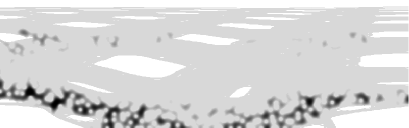
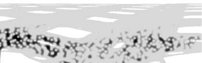
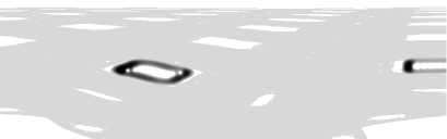
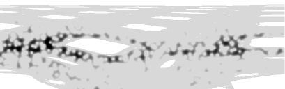
Figure 1: Examples of chaotic (left) and regular (right) states in the Poincaré-Husimi representation. $k_{j}$ ($M$) from top down are: chaotic: $k_{j}$ ($M$) = 2000.0021815 (0.978), 2000.0181794 (0.981), 2000.0000068 (0.989), 2000.0258600 (0.965); regular: $k_{j}$ ($M$) = 2000.0081402 (-0.987), 2000.0777155 ( -0.821), 2000.0786759 ( -0.528), 2000.0112417 ( -0.829). The gray background is the classically chaotic invariant component. We show only one quarter of the surface of section $(s,p)\in[0,{\cal L}/2]\times[0,1]$, because due to the reflection symmetry and time-reversal symmetry the four quadrants are equivalent.

Now the classification of eigenstates can be performed by their projection onto the classical surface of section. As we are very deep in the semiclassical regime we do expect with probability one that either an eigenstate is regular or chaotic, with exceptions having measure zero, ideally. To automate this task we have ascribed to each point on the grid a number $A_{i,j}$ whose value is either $+1$ if the grid point lies within the classical chaotic region or $-1$ if it belongs to a classical regular region. Technically, this has been done as follows. We have taken an initial condition in the chaotic region, and iterated it up to about $10^{10}$ collisions, enough for the convergence (within certain very small distance). Each visited cell $(i,j)$ on the grid has then been assigned value $A_{i,j}=+1$, the remaining ones were assigned the value -1.

The Poincaré Husimi function $H(q,p)$ (19) (normalized) was calculated on the grid points and the overlap index $M$ was calculated according to the definition

$$M=\sum_{i,j}H_{i,j}\;A_{i,j}.$$ (20)

In practice, $M$ is not exactly $+1$ or $-1$, but can have a value in between. The reasons are two, first the finite discretization of the phase space (the finite size grid), and second, the finite wavelength (not sufficiently small effective Planck constant, for which we can take just $1/k_{j}$). If so, the question is, where to cut the distribution of the $M$-values, at the threshold value $M_{t}$, such that all states with $M<M_{t}$ are declared regular and those with $M>M_{t}$ chaotic.

There are two natural criteria: (I) The classical criterion: the threshold value $M_{t}$ is chosen such that we have exactly $\rho_{1}$ fraction of regular levels and $\rho_{2}=1-\rho_{1}$ of chaotic levels. (II) The quantum criterion: we choose $M_{t}$ such that we get the best possible agreement of the chaotic level spacing distribution with the Brody distribution (6), which is expected to capture the dynamical localization effects of the chaotic eigenstates.

4 Results

To begin with we first look at the total energy spectrum $E_{j}=k_{j}^{2}$, for $k_{j}\in[2000,2500]$. The spectral unfolding was done using the Weyl formula with the perimeter corrections. In figure 2a we show the histogram of $N=587653$ level spacings together with the best fitting BRB distribution (2), with $E_{r}$ being Poissonian and $E_{c}$ being the Brody gap probability (8), derived from (6), with the classical $\rho_{1}=0.175$, and the Brody parameter $\beta=0.45$. For the reference the BR distribution (5), the Poisson and the GOE level spacing distributions (3) are shown. In figure 2b we show the $U$-function representation of the level spacing distribution, as introduced by Prosen and Robnik [23] and defined in the Appendix B. It was the $U$-function which was used in finding the best fitting distributions. Whilst in the first case the agreement is perfect, in the $U$-plot we see that the quantally adjusted parameter $\rho_{1}=0.19$ instead of its classical value $0.175$ leads to even better agreement. In this case $\beta=0.47$. Please observe that the deviations here are already extremely small, so the significance of the best fit is of extreme importance.

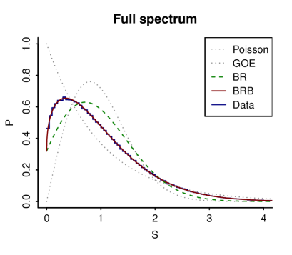
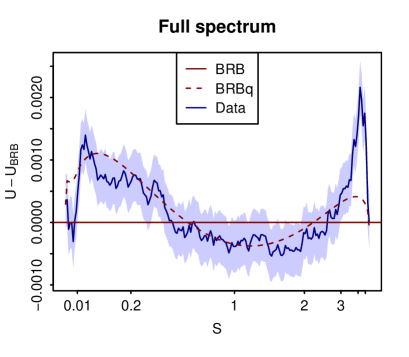
Figure 2: (a; left) The level spacing distribution for the entire spectrum after unfolding for $N=587653$ spacings, with $k_{j}\in[2000,2500]$, in excellent agreement with the BRB distribution with the classical $\rho_{1}=0.175$ and $\beta=0.45$. In the $U$-function plot (b; right), we show $U(data)-U(BRB)$ as a function of $S$, and it is clearly seen that the BRB distribution with the quantally determined $\rho_{1}=0.19$ and $\beta=0.47$ is even better fit to the data (dashed, denoted by BRBq). The belt around the data curve indicates the expected statistical $\pm$ one-sigma error.

Let us now separate the regular and chaotic eigenstates and the corresponding eigenvalues, after unfolding, according to the method described in section 3, using the classical criterion (I). The corresponding threshold value of the index $M$ is found to be $M_{t}=0.431$. The level spacing distributions are shown in figure 3. As we see, we have perfect Brody distribution with $\beta=0.444$ for the chaotic levels and almost pure Poisson for the regular levels.

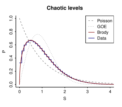
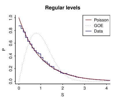
Figure 3: Separation of levels using the classical criterion $M_{t}=0.431$. (a; left) The level spacing distribution for the chaotic subspectrum after unfolding, in perfect agreement with the Brody distribution $\beta=0.444$. (b; right) The level spacing distribution for the regular part of the spectrum, after unfolding, in excellent agreement with Poisson.

In order to make our analysis deeper and more refined we show first the histogram of the $M$-values in figure 4a, where we see the two different threshold values $M_{t}$, namely the classical one at $M_{t}=0.431$, corresponding to $\rho_{1}=0.175$, and the quantum one at $M_{t}=0.75$ in which case we get $\rho_{1}=0.223$. In figure 4b we analyze the goodness of the two fits, Brody and Izrailev. First we define the fit deviation measure as

$$R=\int_{0}^{\infty}P(S)^{2}\left((P(S)-P_{F}(S)\right)^{2}\;dS,$$ (21)

where $P(S)$ describes the data, whilst $P_{F}(S)$ denotes the theoretical distribution fitting the data, namely $F$ stands for Brody or Izrailev. At each chosen threshold value $M_{t}$ we consider the set of chaotic levels for which by definition $M\geq M_{t}$. By performing the best fit at such $M_{t}$ (= threshold $M$) both for Brody and Izrailev, we calculate the fit deviation measure (21) and plot its decadic logarithm as a function of $M_{t}$ in figure 4b. We see that at low $M_{t}$ Izrailev is somewhat better than Brody, but this is the unphysical domain of much too small $M_{t}$. Near the classical threshold $M_{t}=0.431$ they become comparably good, but at increasing the $M_{t}$ Brody exhibits a very sharp and narrow minimum, whilst Izrailev curve increases. This sharp minimum of $R$ for Brody is at the value of $M$ which by definition we called the quantum threshold $M_{t}=0.75$. In addition, we show the $R$ quantity (21) for the Poisson distributioin vs. $M_{t}$, where we see also a deep sharp minimum at $M_{t}\approx 0.8$, thus almost at the quantum threshold $M_{t}=0.75$. The conclusion of this analysis is that by varying the threshold value $M_{t}$ there is a point $M_{t}=0.75$ at which the Brody distribution for all chaotic levels with $M>M_{t}$ is globally the best and also better than Izrailev fit at any $M_{t}$. For logical consistency, it is important that at (almost) the same value of $M_{t}$ the fit of the Poisson distribution for the regular levels with $M<M_{t}$ is globally the best, as is evident from the $R$ plot in figure 4b.

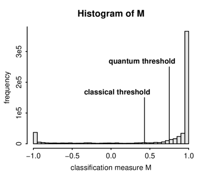
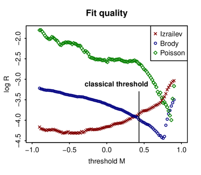
Figure 4: (a; left) Distribution of the index $M$ with the locations of the threshold values of $M$, the classical $M_{t}=0.431$ and the quantum one $M_{t}=0.75$. In the first case classical $\rho_{1}=0.175$, whilst in the second case the quantal $\rho_{1}=0.223$. (b; right) The logarithm of the fit deviation measure $\log_{10}R$, defined in (21), for the Brody and Izrailev distributions for chaotic levels $M>M_{t}$, versus $M_{t}$, and the same for Poisson distribution for the regular levels with $M<M_{t}$.

We show the $U$-function plots for the regular levels and the chaotic levels in figure 5, using the Brody distribution, for the classical and quantum criterions, corresponding to the two different values of $M_{t}$ explained above. In both cases we plot the difference $U(data)-U(ideal)$, so that in case of perfect agreement the line would coincide with the abscissa. We clearly see that the quantum criterion yields noticable better agreement than the classical criterion. Again, it must be emphasized that the agreement is extremely good, and the deviations of $U(data)$ from $U(ideal)$ are very small numbers.

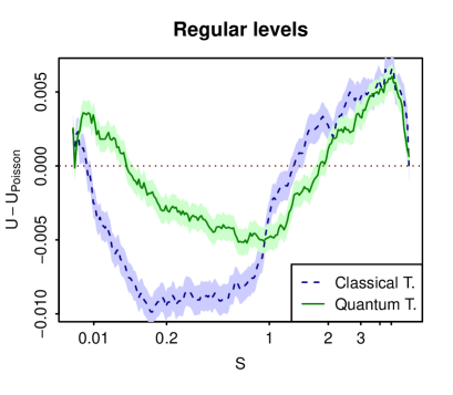
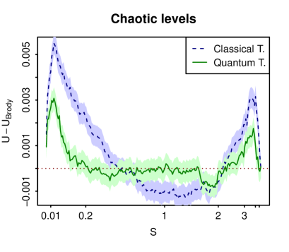
Figure 5: The $U$-function plots as differences $U(data)-U(ideal)$ for the regular and chaotic levels, for both criteria, the classical one and the quantum one. The belts around the data lines indicate the expected statistical $\pm$ one-sigma errors.

Finally, we should comment on the relevance of the Brody distribution. The Brody distribution [43, 44] (6) still has no theoretical foundation, but it definitely captures correctly the effects of dynamical (Chirikov) localization of chaotic eigenstates. This has been recently confirmed by Manos and Robnik [39] in case of the kicked rotator, namely for the quasienergies, and clearly is demonstrated in the present work for the autonomous Hamilton system, exemplified by the 2D billiard that we have chosen for this analysis. It remains as an open theoretical problem to derive the Brody distribution in this context.

Since the Brody distribution is not known theoretically to be the preferred and/or “the right one”, we have considered again also the Izrailev distribution [35, 38, 34] (10), studied very recently also in [39]. Entirely in line with the findings in [39] we found that Brody is much better model of the level spacing distribution than the Izrailev’s one. This is clearly demonstrated in figure 6.

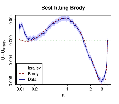
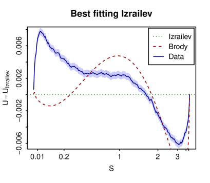
Figure 6: We show the $U$-function plot for the chaotic levels, clearly showing that Brody distribution (dashed) is much better than Izrailev distribution. On the left we show the best fitting Izrailev distribution at the point where Brody is globally the best fit using the quantum threshold $M_{t}=0.75$. On the right we show the Izrailev fit at the point $M_{t}=-0.5$ where it is globally the best, and the best Brody fit at the same $M_{t}=-0.5$, showing that also there the Brody fit is better than Izrailev. This is impressive because the effects are small, and the statistical significance very high. The belt around the data line indicates the expected statistical $\pm$ one-sigma error.

5 Conclusions

We have used a billiard system of the mixed type (11), with $\lambda=0.15$, as introduced in [46]-[47], and have shown that using the Poincaré Husimi functions we can separate the regular and chaotic eigenstates. The successful separation of course also entirely confirms the Berry-Robnik picture [5] of separating the regular and chaotic levels in the semiclassical limit, where the tunneling effects can be neglected. With great and unprecedented statistical significance we have shown that the chaotic levels exhibit Brody level spacing distribution, whilst the regular levels obey Poissonian statistics. This analysis not only confirms the Berry-Robnik picture [5] of conceptually separating the regular and chaotic levels, based on the PUSC and embodied in formula (1), but also demonstrates that the dynamical localization effects of the chaotic eigenstates are very well captured by the Brody distribution, in analogy with the same finding in the Floquet systems, in particular the kicked rotator [34, 39], where the quasienergy spectra are analyzed. One educated guess for the occurrence of fractional power law level repulsion (meaning $0<\beta<1$) in dynamically localized but classically fully chaotic periodic systems is Izrailev’s observation (see e.g. [34] and the references therein), that the joint probability distribution for a Circular Orthogonal Ensemble (COE), which so far as the level spacings are concerned is also GOE, should be generalized in the sense of Dyson for noninteger $\beta$. Of course, this is just a hypothesis, and it certainly cannot indicate theoretically whether Brody or Izrailev distribution should be ”the right one”, leaving us with the empirical studies and conclusions of this work. The analogies and connections between the billiard problem and the Floquet problem have been discussed in more detail in the recent work [63].

Whilst in the kicked rotator the relationship between the localization measure of the eigenstates and the spectral level repulsion (Brody) parameter $\beta$ exists, as proposed by Izrailev, and confirmed by Manos and Robnik, in the time independent Hamilton systems, like the one discussed in the present work, such relationship is lacking and is open for the future work. It involves great numerical efforts.

The theoretical derivation of the Brody level spacing distribution for the dynamically localized eigenstates is thus also an open problem for the future. The billiard systems are not just nice theoretical toy models, but are suitable also for the experimental applications, like in quantum dots, and microwave cavities introduced and studied extensively over decades by H.-J. Stöckmann [1]. We also propose to study from the present point of view the hydrogen atom in strong magnetic field as an example of classical and quantum chaos par excellence, as introduced in [64, 65, 66, 67, 68], although the technical efforts to obtain large stretches of high-lying eigenstates and the corresponding energy levels are much bigger than in billiard systems, where we have a great number of different elegant numerical techniques [69], all of them used in our recent work [24].

Appendix A: The semiclassical condition

Here we calculate the Heisenberg time and the classical transport time for the billiard domain ${\cal B}$ defined in equation (11) with $\lambda=0.15$. According to the leading order of the Weyl formula, which is in fact just the simple Thomas-Fermi rule, we have for the number of levels $N(E)$ below and up to the energy $E$ of a Hamiltonian $H({\bf q},{\bf p})$

$$N(E)=\frac{1}{(2\pi\hbar)^{2}}\int_{H({\bf q},{\bf p})\leq E}d^{2}{\bf q}\;d^{2}{\bf p}.$$ (22)

Since $H={\bf p}^{2}/(2m)$, with constant zero potential energy inside ${\cal B}$, where $m$ is the mass of the billiard point particle, and $H$ is infinite on the boundary $\partial{\cal B}$, we get at once

$$N(E)=\frac{2\pi{\cal A}mE}{(2\pi\hbar)^{2}}.$$ (23)

The density of levels is $\rho(E)=1/(\Delta E)=dN(E)/dE={\cal A}m/(2\pi\hbar^{2})$ and thus the Heisenberg time is

$$t_{H}=2\pi\hbar\rho(E)=\frac{{\cal A}m}{\hbar}.$$ (24)

The classical transport time is denoted by $t_{T}$, and in units of the number of collisions $N_{T}$ can be written as

$$t_{T}=\frac{\bar{l}N_{T}}{v}=\frac{\bar{l}N_{T}}{\sqrt{2E/m}},$$ (25)

where $\bar{l}$ is the mean free path of the billiard particle and $v=\sqrt{2E/m}$ is its speed at the energy $E$. Thus for the ratio $\alpha=t_{H}/t_{T}$ we get

$$\alpha=\frac{t_{H}}{t_{T}}=\frac{{\cal A}k}{N_{T}\bar{l}}$$ (26)

where $k=\sqrt{2mE/\hbar^{2}}$. Taking into account that $\bar{l}\approx\pi{\cal A}/{\cal L}$ (this is so-called Santalo’s formula, see e.g. [70]), we have

$$\alpha=\frac{t_{H}}{t_{T}}=\frac{{\cal L}k}{\pi N_{T}}.$$ (27)

This is a general formula valid for any billiard. In our case ${\cal L}\approx 2\pi$ and we arrive at the final estimate

$$\alpha=\frac{2k}{N_{T}}.$$ (28)

Thus the condition for the occurrence of dynamical localization $\alpha\leq 1$ is now expressed in the inequality

$$k\leq\frac{N_{T}}{2}.$$ (29)

As our levels are in the interval $k\in[2000,2500]$, and since $N_{T}$ is estimated as $N_{T}\approx 10^{5}$, we see that the semiclassical condition (29) is very well satisfied. In figure 7 we explicitly show the growth of the second moment of $p$, namely $\langle p^{2}\rangle$, for an ensemble of 2000 initial conditions uniformly distributed in the chaotic component on the interval $s\in[0,{\cal L}/2]$ with $p=0$, where the averaging is taken over the ensemble and the time. We see that indeed about $N_{T}\approx 10^{5}$ collisions are necessary to reach the saturation value of $\langle p^{2}\rangle$. More detailed study of the relevant transport properties will be published elsewhere [71].

Figure 7: We show the second moment $\langle p^{2}\rangle$ averaged over an ensemble of 2000 initial conditions uniformly distributed in the chaotic component on the interval $s\in[0,{\cal L}/2]$ and $p=0$ as a function of the decadic logarithm of the number of collisions. We see that the saturation value of $\langle p^{2}\rangle$ is reached at about $N_{T}=10^{5}$ collisions.

Appendix B: The U-function representation of the level spacing distribution

First we estimate the expected fluctuation (error) of the cumulative (integrated) level spacing distribution $W(S)$, which contains $N_{s}$ objects. At a certain $S$ we have the probability $W$ that a level is in the interval $[0,W]$ and $1-W$ that it is in the interval $[W,1]$. Assuming binomial probability distribution $P(k)$ of having $k$ levels in the first and $N_{s}-k$ levels in the second interval we have

$$P(k)=\frac{N_{s}!}{k!(N_{s}-k)!}W^{k}(1-W)^{N_{s}-k}.$$ (30)

Then the average values are equal to

$$<k>=N_{s}W,\;\;\;<k^{2}>=N_{s}W+N_{s}(N_{s}-1)W^{2},$$ (31)

and the variance

$$V(k)=<k^{2}>-<k>^{2}=N_{s}W(1-W).$$ (32)

But the probability $W$ is estimated in the mean as $k/N_{s}$. Its variance is

$$V(W)=V\left(\frac{k}{N_{s}}\right)=\frac{1}{N_{s}^{2}}V(k)=\frac{W(1-W)}{N_{s}}$$ (33)

and therefore the estimated error of $W$ (standard deviation, the square root of the variance) is given by

$$\delta W=\sqrt{V(W)}=\sqrt{\frac{W(1-W)}{N_{s}}}.$$ (34)

Transforming now from $W(S)$ to

$$U(S)=\frac{2}{\pi}\arccos\sqrt{1-W(S)},$$ (35)

we show in a straightforward manner that

$$\delta U=\frac{1}{\pi\sqrt{N_{s}}}$$ (36)

and is indeed independent of $S$. From the (choice of the constant pre-factor in the) definition (35) one sees that both $U(S)$ and $W(S)$ go from $0$ to $1$ as $S$ goes from $0$ to infinity.

References

References

- [1] Stöckmann H.-J. 1999 Quantum Chaos - An Introduction (Cambridge: Cambridge University Press).
- [2] Haake F 2001 Quantum Signatures of Chaos (Berlin: Springer)
- [3] Robnik M 1998 Nonl. Phen. in Compl. Syst. (Minsk) 1 1
- [4] Percival I C 1973 J. Phys. B: At. Mol. Phys. 6 L229
- [5] Berry M V and Robnik M 1984 J. Phys. A: Math. Gen. 17 2413
- [6] Mehta M L 1991 Random Matrices (Boston: Academic Press)
- [7] Guhr T, Müller-Groeling A and Weidenmüller H A 1998 Phys. Rep. 299 Nos. 4-6 189
- [8] Bohigas O, Giannoni M.-J and Schmit C 1984 Phys. Rev. Lett. 52 1
- [9] Casati G, Valz-Gris F and Guarneri I 1980 Lett. Nuovo Cimento 28 279
- [10] Robnik M and Berry M V 1986 J. Phys. A: Math. Gen. 19 669
- [11] Robnik M 1986 Lect. Notes Phys. 263 120
- [12] Berry M V 1985 Proc. Roy. Soc. Lond. A 400 229
- [13] Gutzwiller M C 1990 Chaos in Classical and Quantum Mechanics (Berlin: Springer) and references therein
- [14] Sieber M and Richter K 2001 Phys. Scr. T90 128
- [15] Müller S, Heusler S, Braun P, Haake F and Altland A 2004 Phys. Rev. Lett. 93 014103
- [16] Heusler S, Müller S, Braun P and Haake F 2004 J. Phys.A: Math. Gen. 37 L31
- [17] Müller S, Heusler S, Braun P, Haake F and Altland A 2005 Phys. Rev. E 72 046207
- [18] Müller S, Heusler S, Altland A, Braun P, and Haake F 2009 New J. of Phys. 11 103025
- [19] Robnik M and Veble G 1998 J. Phys. A: Math. Theor. 31 4669
- [20] Berry M V 1977 J Phys. A: Math. Gen. 12 2083
- [21] Prosen T and Robnik M 1999 J. Phys. A: Math. Gen. 32 1863
- [22] Prosen T and Robnik M 1994 J. Phys. A: Math. Gen. 27 L459
- [23] Prosen T and Robnik M 1994 J. Phys. A: Math. Gen. 27 8059
- [24] Batistić B and Robnik M 2010 J. Phys. A: Math. Theor. 43 215101
- [25] Veble G, Robnik M and Liu Junxian 1999 J. Phys. A: Math. Gen. 32 6423
- [26] Prosen T and Robnik M 1993 J. Phys. A: Math. Gen. 26 2371
- [27] Prosen T and Robnik M 1993 J. Phys. A: Math. Gen. 26 1105
- [28] Prosen T 1998 J. Phys. A: Math. Gen. 31 L345
- [29] Prosen T 1998 J. Phys. A: Math. Gen. 31 7023
- [30] Grossmann S and Robnik M 2007 J. Phys. A: Math. Theor. 40 409
- [31] Grossmann S and Robnik M 2007 Z. Naturforschung A 62 471
- [32] Vidmar G, Stöckmann H.-J., Robnik M, Kuhl U, Höhmann R and Grossmann S 2007 J. Phys. A: Math. Theor. 40 13883
- [33] Casati G, Chirikov B, Ford J and Izrailev F M 1979 Lect. Notes Phys. 93 334
- [34] Izrailev F M 1990 Phys. Rep. 196 299
- [35] Izrailev F M 1988 Phys. Lett. A 134 13
- [36] Izrailev F M 1986 Phys. Rev. Lett. 56 541
- [37] Izrailev F M 1987Phys. Lett. A 125 250
- [38] Izrailev F M 1989 J. Phys. A: Math. Gen. 22 865
- [39] Manos T and Robnik M 2013 Phys. Rev. E 87 062905-1 - 062905-17 (ArXiv: 1301.4187)
- [40] Prosen T 2000 in Proceedings of the International School of Physics ”Enrico Fermi”, Course CXLIII, Eds. G. Casati, I. Guarneri and U. Smilyanski (Amsterdam: IOS Press) p 473
- [41] Li Baowen and Robnik M 1995 J. Phys. A: Math. Gen. 28 4843
- [42] Barnett A H and Betcke T 2007 CHAOS 17 043125
- [43] Brody T A 1973 Lett. Nuovo Cimento 7 482
- [44] Brody T A, Flores J, French J B, Mello P A, Pandey A and Wong S S M 1981 Rev. Mod. Phys. 53 385
- [45] Casati G, Izrailev F and Molinari L 1991 J. Phys. A: Math. Gen. 24 4755
- [46] Robnik M 1983 J. Phys. A: Math. Gen. 16 3971
- [47] Robnik M 1984 J. Phys. A: Math. Gen. 17 1049
- [48] Markarian R 1993 Nonlinearity 6 819
- [49] Lazutkin V F 1981 Convex billiard and eigenfunctions of the Laplace operator (University of Leningrad) in Russian
- [50] Lazutkin V F 1991 KAM Theory and Semiclassical Approximations to Eigenfunctions (Berlin: Springer)
- [51] Hayli A, Dumont T, Moulin-Ollagier J and Strelcyn J M 1987 J. Phys. A: Math. Gen. 20 3237
- [52] Dobnikar J 1996 Diploma Thesis, CAMTP University of Maribor and FMF University of Ljubljana, unpublished
- [53] Li Baowen and Robnik M 1994 J. Phys. A: Math. Gen. 27 5509
- [54] Robnik M, Dobnikar J, Rapisarda A, Prosen T and Petkovšek M 1997 J. Phys. A: Math. Gen. L803
- [55] Bäcker A, Fürstberger S and Schubert R 2004 Phys. Rev. E 70 036204
- [56] Berry M V and Wilkinson M 1984 Proc. Roy. Soc. Lond. A 392 15
- [57] Wigner E P 1932 Phys. Rev. 40 749
- [58] Husimi K 1940 Proc. Phys. Math.. Soc. Jpn. 22 264
- [59] Crespi B, Perez G and Chang S.-J. 1993 Phys. Rev. E 47 986
- [60] Tualle J M and Voros A 1995 Chaos, Solitons and Fractals 5 1085
- [61] Simonotti F P, Vergini E and Saraceno M 1997 Phys. Rev. E 56 3859
- [62] Vergini E and Saraceno M 1995 Phys. Rev. E 52 2204
- [63] Batistić B, Manos T and Robnik M 2013 Europhys. Lett. 102 50008
- [64] Robnik M 1981 J. Phys. A: Math. Gen. 14 3195-3216
- [65] Robnik M 1982 J. Phys. Colloque C2 43 29
- [66] Hasegawa H, Robnik M and Wunner G 1989 Prog. Theor. Phys. Suppl. (Kyoto) 98 198-286
- [67] Wintgen D and Friedrich H 1989 Phys. Rep. 183 38
- [68] Ruder H, Wunner G, Herold H and Geyer F 1994 Atoms in Strong Magnetic Fields (Heidelberg: Springer)
- [69] Veble G, Prosen T and Robnik M 2007 New J. Phys. 9 1
- [70] Santaló L A 1976 Integral Geometry and Geometric Probability (Reading, Mass.: Addison-Wesley Publ. Co.)
- [71] Batistić B and Robnik M 2013 to be submitted