Simulating a dual beam combiner at SUSI for narrow-angle astrometry

Abstract

The Sydney University Stellar Interferometer (SUSI) has two beam combiners, i.e. the Precision Astronomical Visible Observations (PAVO) and the Microarcsecond University of Sydney Companion Astrometry (MUSCA). The primary beam combiner, PAVO, can be operated independently and is typically used to measure properties of binary stars of less than 50 milliarcsec (mas) separation and the angular diameters of single stars. On the other hand, MUSCA was recently installed and must be used in tandem with the former. It is dedicated for microarcsecond precision narrow-angle astrometry of close binary stars. The performance evaluation and development of the data reduction pipeline for the new setup was assisted by an in-house computer simulation tool developed for this and related purposes. This paper describes the framework of the simulation tool, simulations carried out to evaluate the performance of each beam combiner and the expected astrometric precision of the dual beam combiner setup, both at SUSI and possible future sites.

1 Introduction

A dual beam combiner setup was recently installed in SUSI. The main role of the new setup is to perform high precision narrow-angle astrometry of close binary stars. The relative position of one star on the celestial sphere with respect to another in a binary system can be determined by measuring the separation (in optical delay) of their fringe packets formed by an optical long baseline interferometer like SUSI. The accuracy of the projected separation of the binary star systems obtained from this method is determined by the uncertainty of the optical delay measurement. A more accurate measurement of the optical delay of a fringe packet can be made by measuring the phase delay of the fringes instead of the group delay (Lawson et al, 2000).

Now, if the measurements are to be carried out from the ground then the position of the pair of fringe packets must first be stabilized because their positions are not static but constantly changing due to atmospheric turbulence. This can be achieved using a technique called phase-referencing (PR) (Colavita, 1992; Shao and Colavita, 1992). In this technique, two beam combiners are required. The phase delay of one fringe packet is measured accurately in the presence of atmospheric turbulence with one beam combiner (usually called the fringe tracker) and then fed-forward into another companion beam combiner to stabilize the position of the same or another fringe packet. This technique was demonstrated with PHASES (Muterspaugh et al, 2010) at PTI (Colavita et al, 1999) in the near infra-red wavelengths which had achieved an astrometric precision of 35$\mu$as (with separation less than 1^′′ close binaries) within 70 minutes of observation time (Lane and Muterspaugh, 2004).

The dual beam combiner setup in SUSI is specifically designed to do the same (phase-referencing observations). The main beam combiner at SUSI, namely PAVO  is used as the fringe tracker to measure the phase delay of the fringes of the primary star in the binary system in real time and the companion beam combiner, namely MUSCA, is used to simultaneously record either the fringes of the primary or the secondary star. This setup is similar to PHASES where both beam combiners receive the same pair of starlight beams from the siderostats and observe the same field of view ($<2^{\prime\prime}$) of the sky. However in many other ways it is different. Firstly, PAVO and MUSCA operate in the visible wavelengths. Secondly, each beam combiner operates at a slightly different bandwidth compared to the other. Thirdly, the phase-referencing of stellar fringes are carried out in post-processing which eliminates the need for a feedback servo loop in MUSCA. Lastly, MUSCA observes only one stellar fringe packet at a time but can switch between a pair of fringe packets of a binary star during observation.

With the introduction of MUSCA into SUSI, the existing data reduction pipeline was also upgraded to support the dual beam combiner configuration. The software development, which mainly involved putting in additional features to estimate phase delay of stellar fringes and to carry out a non-real time phase-referencing operation, was greatly assisted by an in-house computer simulation framework. The framework and its usage are described in this paper. Firstly, Section 2 gives a general overview of the simulation framework. Subsequently, Sections 3, 4 and 5 describe models of fringes employed by the simulators to generate the test data sets while Section 6 describes a method that was used to include the effect of atmospheric turbulence in the simulation. Lastly Section 7 shows the output of several dual beam combiner simulations and the expected performance of the instruments.

2 Simulators and the framework

Two simulators, which are computer models of the PAVO and MUSCA beam combiners, are developed to generate a set of simulated interferograms of each beam combiner based on user-specified inputs. The simulators were written in the Interactive Data Language (IDL) but the design concepts and algorithms described here can be implemented in any other languages. Both simulators can read the same set of user-specified inputs and by doing so allow users to simulate a dual beam combiner operation in which stellar fringes are recorded by the actual instruments simultaneously in real time. The simulated interferograms can then be used to test the fringe visibility squared ($V^{2}$) estimation and the phase-referencing algorithm of the upgraded data reduction pipeline (Kok et al, 2012). By comparing the user-specified input and the simulator output, especially the estimated $V^{2}$ since it is the main science observable of PAVO, the accurateness of the estimation and the performance of the dual beam combiner setup can be assessed. Fig. 1 illustrates the data reduction pipeline test bench which shows the usage of the two simulators developed in this work.

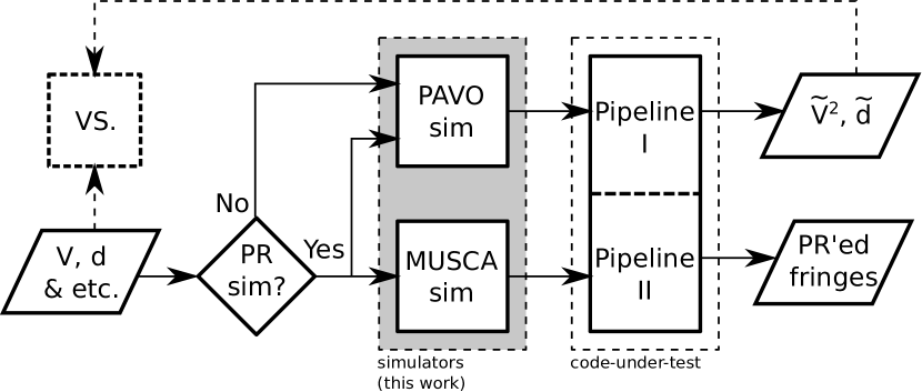
Figure 1: Logical flow diagram of the data reduction pipeline test bench.

An overall logical flow of both simulators is illustrated in Fig. 2. Simulation begins with a generic model of two or more pupils. They are then customized according to the optics of individual beam combiner. Additional and optional phase noise to simulate the effect of atmospheric turbulence can be included before the customization of the pupils. Then user-specified inputs are processed, e.g. to determine the number of interferograms (referred to as frames in the flow diagram) to be generated or the visibility and phase delay of the fringes to be simulated. After generating the required frame either by coherent or incoherent combination of the pupils, depending on the type of frame (refer Section 3.3), e.g. science (S-), foreground (F-), ratio (R-) or dark (D-) frame, the amplitude of the combined pupil is converted into photon counts and subsequently into the detector read-out units (ADU). The detector read-out noise is also included into the simulator output. The simulated data is then saved into a file of appropriate format. The simulation finishes when all the required frames are generated. The details of each stage of the logical flow are discussed in the subsequent sections.

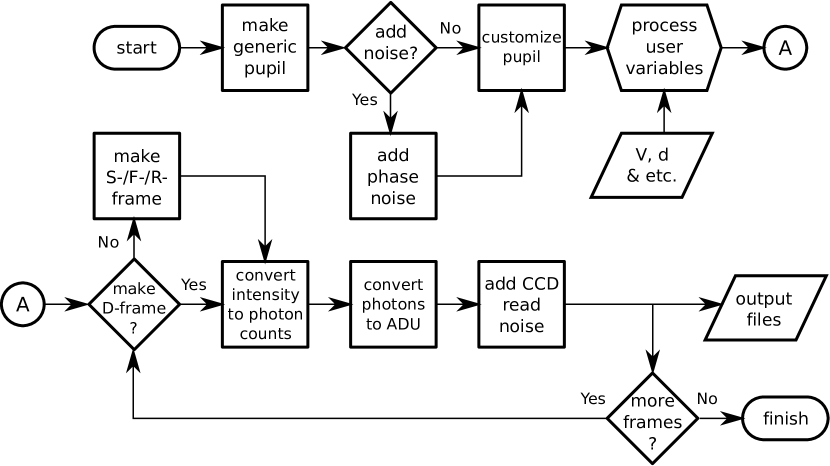
Figure 2: Logical flow diagram of the PAVO and MUSCA simulators.

3 The PAVO simulator

The PAVO beam combiner is a multi-axially aligned Fizeau-type interferometer. But unlike a typical Fizeau interferometer, PAVO forms spatially modulated interference fringes in the pupil plane of the interferometer and then spectrally disperses the fringes with an integral field unit. It also employs spatial filtering in its image plane and an array of cylindrical lenslet to utilize the full multi-r₀ aperture of the siderostats at SUSI. The lenslet array fragments the pupil of the siderostats into several segments so that fringes from different parts of the pupil can be measured separately. The schematic diagram of the PAVO beam combiner is shown in Fig. 3. It combines starlight beams from any 2 of the 11 siderostats (Davis et al, 1999) at one time. Despite that, the PAVO simulator developed in this work is able to simulate higher order beam combination (i.e. 3 and more beams simultaneously) because the optical design of PAVO at SUSI is an adaptation of a twin instrument at the CHARA array on Mount Wilson, California (McAlister et al, 2005), which has the capability of combining starlight beams from up to 3 telescopes. The original optical design of PAVO at CHARA and the modified version at SUSI have been discussed in detail by Ireland et al (2008) and Robertson et al (2010) respectively.

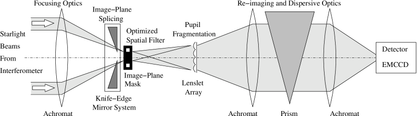
Figure 3: Schematic diagram of the PAVO beam combiner at SUSI.

3.1 Input and output of the simulator

There are more than 20 input parameters to the PAVO simulator with the more critical ones listed in Table 1. Some input parameters are common to the MUSCA simulator which will be described in Section 4. The main output of the simulator is a set of FITS formatted files which contain images of simulated interferograms, hereinafter referred to as frames, as well as header information (e.g. timestamp, fringe lock status, etc) as would be recorded by the PAVO camera. There are four different types of frames recorded by the camera during actual observations. There are the science, ratio, foreground and dark frames. Examples of each of these frames are shown in Fig. 4. Each frame, except the dark, contains images of the spectrally dispersed (horizontally in the figure) pupil as sampled by an array of lenslets. The number of lenslets, $N_{\rm{LL}}$, is different between PAVO at SUSI and at CHARA. The example shown in Fig. 4 is of the former which has the lenslets arranged in a one-dimensional array and there are 4 lenslets per pupil. The left pupil is for science while the middle and right pupils are used for tip-tilt correction and therefore are ignored in the simulation. Frames of PAVO at CHARA contains only the science pupil.

Table 1: Input parameters for the PAVO (P) and MUSCA (M) simulators

Name	Simulators	Description
$t_{\rm{START}}$	P,M	Start of simulation in Julian date
$t_{\rm{STEP}}$	P,M	Exposure time of camera/photodetector
$N_{\rm{S-FITS}}$	P	Number of science type FITS to generate
$N_{\rm{R-FITS}}$	P	Number of ratio type FITS to generate
$N_{\rm{F-FITS}}$	P	Number of foreground type FITS to generate
$N_{\rm{D-FITS}}$	P	Number of dark type FITS to generate
$N_{\rm{MED}}$	P,M	Number and types of optical media
$\boldsymbol{\zeta}$	P,M	Astrometric OPD in m
$N_{\rm{TEL}}$	P,M	Number of telescopes
$\mathbf{B}$	P,M	Details of telescopes (e.g. baselines) to be used
$m_{V}$	P,M	Magnitude of source in V band
$\mathbf{V}$	P,M	Model complex visibility of source
$\mathbf{D},\mathbf{d}$	P,M	Offset of $\boldsymbol{\zeta}$ in m
$r_{0}$	P,M	Fried parameter in m
$\sigma_{r_{0}}^{-1}$	P,M	Wavelength in which $r_{0}$ is specified ($\mu$m)
$\tau_{0}$	P,M	Coherence time in milliseconds
$L_{0}$	P,M	Outer scale of atmospheric turbulence in m
$t_{\rm{STEP}}$	M	Time interval between steps
$N_{\rm{STEP}}$	M	Number of steps per scan
$N_{\rm{SCAN}}$	M	Number of scan to simulate
$L_{\rm{SCAN}}$	M	Length of a scan in $\mu$m

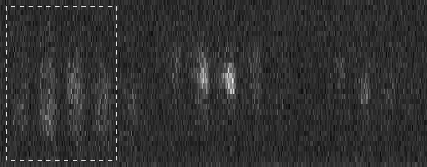
(a)

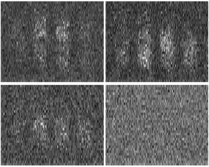
(b)

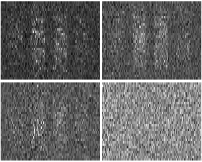
(c)

Figure 4: (a) An example of real on-sky data of $\alpha$ Gru recorded by the PAVO camera. It contains images of spectrally dispersed (horizontally) pupils as sampled by an array of four lenslets. The science pupil on the left (indicated by the dotted box) of the frame is where fringes are formed by a pair of overlapped pupils. The pupils in the middle and left of the frame are used for tip-tilt control. They are ignored and will not be generated during simulation. The images of the science pupil for different frame types are shown in (b) and (c). The images, from left to right and top to bottom, belong to four different types of frames, namely science, foreground, ratio and dark respectively. The images in (b) are recorded by the camera while those in (c) are generated by the simulator. The convention adopted by the mathematics in this paper takes the vertical axis, which is the fringes direction, as the $x$-axis and the horizontal axis, which is the spectral channel direction, as the $y$-axis.

3.2 Model pupil

Before the pupils are combined to form fringes, they are first spatially filtered in the image plane with square apertures (hereinafter referred to as the PAVO mask), one for each beam, to remove high spatial frequency noise arising as a consequence of atmospheric turbulence and optical aberration. A pupil from a telescope is modeled by a square matrix, $\tilde{\mathbf{P}}$, of size $N_{\rm{FFT}}\times N_{\rm{FFT}}$,

$$\begin{split}\tilde{\mathbf{P}}&=\left\{\begin{array}[]{l l}\mathbf{J_{N_{\rm{FFT}},N_{\rm{FFT}}}}&\quad;\text{perfect wavefront}\\ \mathbf{J_{N_{\rm{FFT}},N_{\rm{FFT}}}}\circ\exp\left(i\boldsymbol{\varphi}\right)&\quad;\text{corrugated wavefront}\\ \end{array}\right.\\ \end{split}$$ (1)

where $\mathbf{J}$ represents a unit matrix consisting of all 1s of size (row$\times$column) indicated by its subscript and the phase component is either zero or $\boldsymbol{\varphi}$ so as to represent a perfect or corrugated wavefront. A corrugated wavefront due to atmospheric turbulence will be elaborated in Section 6. The notation $\circ$ is the Hadamard or the element-by-element multiplication operator of two matrices. The model of a spatially filtered pupil, $\mathbf{P^{\prime}}$, is then,

$$\begin{split}\mathbf{P^{\prime}}&=\mathcal{FT}^{-1}\left\{\Box\circ\mathcal{FT}\left\{\bigcirc\circ\tilde{\mathbf{P}}\right\}\right\}\\ \end{split}$$ (2)

where $\bigcirc$ and $\Box$ are square matrices of the same size which define a circular pupil and the spatial filter respectively. Each element in the matrices is defined as,

$$\begin{split}\bigcirc_{u,v}&=\left\{\begin{array}[]{l l}1&\quad;\text{if}\;\sqrt{(u-N_{\rm{FFT}}/2)^{2}+(v-N_{\rm{FFT}}/2)^{2})}\leq N_{\rm{DIA}}/2\\ 0&\quad;\text{otherwise}\\ \end{array}\right.\\ \Box_{x,y}&=\left\{\begin{array}[]{l l}1&\quad;\text{if}\;|x-N_{\rm{FFT}}/2|\leq N_{\rm{MASK}}/2\;\text{and}\;|y-N_{\rm{FFT}}/2|\leq N_{\rm{MASK}}/2\\ 0&\quad;\text{otherwise}\\ \end{array}\right.\\ \end{split}$$ (3)

where $N_{\rm{DIA}}$ and $N_{\rm{MASK}}$ are relative sizes of the diameter of the telescopes and the width of the PAVO mask respectively. $N_{\rm{FFT}}$, $N_{\rm{DIA}}$ and $N_{\rm{MASK}}$ take only integer values. The ratio of the width of the mask to the size of the image varies with the wavelength of light and is defined in Eq. (4). In this paper the wavelength of light is always represented by its reciprocal, or wavenumber, $\sigma$ or $\sigma_{j}$, where $j$ is the index of vector $\boldsymbol{\sigma}$ which represents a range of wavenumbers applicable to PAVO. The wavelength scaling factor in Eq. (4) is derived based on the $f$-ratio of the beam and the distance of the PAVO mask from the pupil plane. The different values between PAVO at SUSI and CHARA means the optical setup at the two interferometers are not exactly the same. The simulator keeps the denominator of the left-hand side (LHS) of Eq. (4) constant and varies $N_{\rm{MASK}}$ at different wavelengths of light to satisfy the equation.

$$\begin{split}\frac{N_{\rm{MASK}}}{N_{\rm{FFT}}/N_{\rm{DIA}}}&\approx\left\{\begin{array}[]{l l}1.7\sigma_{j}&\quad;\text{SUSI}\\ 8.5\sigma_{j}&\quad;\text{CHARA}\\ \end{array}\right.\\ \end{split}$$ (4)

With $N_{\rm{FFT}}$ and $N_{\rm{DIA}}$ typically set to 256 and 114 respectively, the range of values of $N_{\rm{MASK}}$ is 5–7 for SUSI and 22–30 for CHARA.

Before a model pupil is used to form fringes, it is down-sampled to the size of an actual image taken by the PAVO camera, which is $N_{\rm{X}}\times N_{\rm{LL}}$, where $N_{\rm{X}}$ is the number of pixels in the $x$-axis and $N_{\rm{LL}}$ is the number of lenslets in the $y$-axis. The values of each parameter are listed in Table 2. As a result, the model pupil becomes,

$$\begin{split}\mathbf{P}&=\frac{1}{N_{\rm{X}}N_{\rm{LL}}}\boldsymbol{\mathcal{I}}\mathbf{{}^{T}_{N_{\rm{FFT}},N_{\rm{X}}}}\;\mathbf{P^{\prime}}\;\boldsymbol{\mathcal{I}}\mathbf{{}_{N_{\rm{FFT}},N_{\rm{LL}}}}\;\end{split}$$ (5)

where $\boldsymbol{\mathcal{I}}\mathbf{{}_{M,N}}$ is a M$\times$N matrix,

$$\begin{split}\boldsymbol{\mathcal{I}}\mathbf{{}_{M,N}}&=\begin{bmatrix}\mathbf{J_{M/N,1}}&0&\cdots&0\\ 0&\mathbf{J_{M/N,1}}&\cdots&0\\ \vdots&\vdots&\ddots&\vdots\\ 0&0&\cdots&\mathbf{J_{M/N,1}}\\ \end{bmatrix}\end{split}$$ (6)

and $\mathbf{J_{M/N,1}}$ is a $M/N\times 1$ unit matrix consisting of all 1s. This simple down-sampling only works if $M$ is an integer multiple of $N$. For example, to down-sample a 6$\times$6 matrix $\mathbf{P}^{\prime}$ to a 2$\times$3 matrix $\mathbf{P}$, the following operation can be applied,

$$\begin{split}\mathbf{P}&=\frac{1}{6}\begin{bmatrix}1&0\\ 1&0\\ 1&0\\ 0&1\\ 0&1\\ 0&1\\ \end{bmatrix}^{\mathbf{T}}\begin{bmatrix}P_{1,1}^{\prime}&P_{1,2}^{\prime}&\cdots&P_{1,6}^{\prime}\\ P_{2,1}^{\prime}&P_{2,2}^{\prime}&\cdots&P_{2,6}^{\prime}\\ \vspace{-0.4em}\\ \vdots&\vdots&\ddots&\vdots\\ \vspace{-0.4em}\\ P_{6,1}^{\prime}&P_{6,2}^{\prime}&\cdots&P_{6,6}^{\prime}\\ \end{bmatrix}\begin{bmatrix}1&0&0\\ 1&0&0\\ 0&1&0\\ 0&1&0\\ 0&0&1\\ 0&0&1\\ \end{bmatrix}\end{split}$$ (7)

where the first and the last matrices on the right-hand side (RHS) are $\boldsymbol{\mathcal{I}}\mathbf{{}_{6,2}}$ and $\boldsymbol{\mathcal{I}}\mathbf{{}_{6,3}}$ respectively.

The values of the physical parameters in Eq. (4), Eq. (5) and other equations in this section are listed in Table 2.

Table 2: Specification of PAVO

Parameter	Notation	PAVO@CHARA	PAVO@SUSI
Number of spectral channels	$N_{\rm{\sigma}}$	19	21
Spectral range ($\mu$m-1)	$\boldsymbol{\sigma}$	1/0.88 – 1/0.63	1/0.80 – 1/0.53
Number of lenslets	$N_{\rm{LL}}$	16	4
Number of pixels in x-axis	$N_{\rm{X}}$	128	32
FOV to pupil size ratio	$\tilde{R}$	5.8	1.8

3.3 Simulating various types of frames

Different types of frames are generated using different combinations of model pupils described in Section 3.2. Sets of 50 frames are saved into a FITS file. Each FITS file has a timestamp of,

$$t_{\alpha}=t_{\rm{START}}+50\times\alpha t_{\rm{STEP}}$$ (8)

where $\alpha$ is the number of FITS files already generated before the current one. The typical value of $t_{\rm{STEP}}$ for PAVO at SUSI and CHARA is 5ms and 8ms respectively. The number of files to be generated for each type of frame is determined by the user.

3.3.1 Science frames

The science frames are generated using two or three pupils, depending on the number of telescopes in use. Simulation of PAVO at CHARA can use up to three. In reality the pupils are aligned to overlap each other and combined to produce spatially modulated fringes across the pupils. The model intensity across the overlapped pupils at one particular wavelength is given as,

$$\begin{split}\mathbf{F}&=w_{j}\sum_{\theta=1}^{N_{\rm{TEL}}}\sum_{\tilde{\theta}=1}^{N_{\rm{TEL}}}V_{\theta,\tilde{\theta}}\,a_{\theta}\mathbf{P}^{(\theta)}\circ a_{\tilde{\theta}}\overline{\mathbf{P}}^{(\tilde{\theta})}\,\circ\exp\left(i\mathbf{\Phi}^{(\theta,\tilde{\theta})}\right)\\ \end{split}$$ (9)

where the notation $\overline{\mathbf{P}}$ represents the complex conjugate of the variable $\mathbf{P}$. The indices $\theta$ and $\tilde{\theta}$ denote one of the several pairs of telescopes used in the simulation ($N_{\rm{TEL}}$) while $a_{\theta}$ denotes the weighted amplitude of $\mathbf{P}^{(\theta)}$ such that,

$$\begin{split}a_{1}^{2}+a_{2}^{2}+\cdots+a_{N_{\rm{TEL}}}^{2}=1\end{split}$$ (10)

This condition has no physical reason but is imposed for the convenience of scaling the normalize intensity to the right photon rate in Section 5. The term $w_{j}$ states the relative intensity of the summation in Eq. (9) at one wavelength while the vector $\mathbf{w}$ which $w_{j}$ is a part of describes the spectrum of the light source and the bandpass profile of PAVO,

$$\begin{split}\mathbf{w}=\begin{bmatrix}w_{1}&w_{2}&\cdots&w_{N_{\sigma}}\end{bmatrix}\;\;;\text{where }\mathbf{wJ_{N_{\sigma},1}}=1\end{split}$$ (11)

This term can easily be customized by user according to the need of a simulation. However, the results shown in Section 7 were simulated with a smooth-edged top hat function for $\mathbf{w}$. The model of fringes, $\mathbf{F}$, is expressed in this form in order to allow a model of complex fringe visibility, $V_{\theta,\tilde{\theta}}$, to be applied to the pairs of pupils. The complex fringe visibility matrix, which is a user supplied input, is defined as,

$$\begin{split}\mathbf{V}&=\begin{bmatrix}1&V(\sigma_{j}B_{1,2})&\cdots&V(\sigma_{j}B_{1,N_{\rm{TEL}}})\\ \overline{V}(\sigma_{j}B_{1,2})&1&\cdots&V(\sigma_{j}B_{2,N_{\rm{TEL}}})\\ \vdots&\vdots&\ddots&\vdots\\ \overline{V}(\sigma_{j}B_{1,N_{\rm{TEL}}})&\overline{V}(\sigma_{j}B_{2,N_{\rm{TEL}}})&\cdots&1\\ \end{bmatrix}\\ \end{split}$$ (12)

where each off diagonal element represents the fringe visibility of a model light source at a given wavelength and baseline. The term $B_{\theta,\tilde{\theta}}$ is the magnitude of a baseline vector $\vec{B}_{\theta,\tilde{\theta}}$ formed by a pair of telescopes $\theta$ and $\tilde{\theta}$. Lastly the matrix $\mathbf{\Phi}$ represents an additional phase difference between the two pupils and it is used to model the difference in piston and tilt in the wavefront of the pupils.

$$\begin{split}\mathbf{\Phi}^{(\theta,\tilde{\theta})}&=2\pi\sigma_{j}\left(\zeta_{\theta,\tilde{\theta}}+[\mathbf{N}]_{j,*}\mathbf{z}^{(\theta,\tilde{\theta})}+D_{\theta,\tilde{\theta}}+N_{j,1}S_{\theta,\tilde{\theta}}\tilde{R}\mathbf{x}\mathbf{J_{1,N_{\rm{LL}}}}\right)\\ \end{split}$$ (13)

The first three terms in Eq. (13) represent the piston term. The first term $\zeta_{\theta,\tilde{\theta}}$ is the astrometric OPD due to the position of the target star with respect to the baseline $B_{\theta,\tilde{\theta}}$ while the second term $[\mathbf{N}]_{j,*}\mathbf{z}^{(\theta,\tilde{\theta})}$ is the optical path of the delay line used to compensate the astrometric OPD.

$$\begin{split}\boldsymbol{\zeta}&=\begin{bmatrix}0&\hat{s}\cdot\vec{B}_{1,2}&\cdots&\hat{s}\cdot\vec{B}_{1,N_{\rm{TEL}}}\\ -\hat{s}\cdot\vec{B}_{1,2}&0&\cdots&\hat{s}\cdot\vec{B}_{2,N_{\rm{TEL}}}\\ \vdots&\vdots&\ddots&\vdots\\ -\hat{s}\cdot\vec{B}_{1,N_{\rm{TEL}}}&-\hat{s}\cdot\vec{B}_{2,N_{\rm{TEL}}}&\cdots&0\end{bmatrix}\\ \end{split}$$ (14)

The optical delay line can comprise of various optical media. The types of optical media are specified by the user but practically it is not more than 4 different types (e.g. vacuum, air and two types of glass, BK7 or F7). The refractive indices for each medium at the wavenumbers of PAVO are calculated using values and constants obtained from Tango (1990). The notation $[\mathbf{N}]_{j,*}$ represents the $j$-th row of the refractive indices matrix, $\mathbf{N}$, where,

$$\begin{split}\mathbf{N}&=\begin{bmatrix}n_{1}(\sigma_{1})&n_{2}(\sigma_{1})&\cdots&n_{N_{\rm{MED}}}(\sigma_{1})\\ n_{1}(\sigma_{2})&n_{2}(\sigma_{2})&\cdots&n_{N_{\rm{MED}}}(\sigma_{2})\\ \vdots&\vdots&\ddots&\vdots\\ n_{1}(\sigma_{N_{\sigma}})&n_{2}(\sigma_{N_{\sigma}})&\cdots&n_{N_{\rm{MED}}}(\sigma_{N_{\sigma}})\\ \end{bmatrix}\end{split}$$ (15)

and $n_{i}$ is the refractive index of one optical medium. In order to set a convention, the first medium ($i=1$) is air. Each element in the column vector $\mathbf{z}$ represents the optical path length of each medium and to optimally compensate a given astrometric OPD the values of $\mathbf{z}$ are calculated using the method described by Tango (1990). The third term in Eq. (13) is an offset term to allow users to simulate a non-optimally compensated astrometric OPD. The user input matrix $\mathbf{D}$ is defined as,

$$\begin{split}\mathbf{D}&=\begin{bmatrix}0&d_{1,2}&\cdots&d_{1,N_{\rm{TEL}}}\\ -d_{1,2}&0&\cdots&d_{2,N_{\rm{TEL}}}\\ \vdots&\vdots&\ddots&\vdots\\ -d_{1,N_{\rm{TEL}}}&-d_{2,N_{\rm{TEL}}}&\cdots&0\end{bmatrix}\\ \end{split}$$ (16)

where $d_{1,2}$ for example is the OPD offset for baseline $B_{1,2}$.

The last term in Eq. (13) is the OPD caused by the differential wavefront tilt between a pair of pupils at the pupil plane. It is proportional to the separation of the apertures on the PAVO mask and inversely proportional to the distance of the pupil plane from the mask. $S_{\theta,\tilde{\theta}}$ is the ratio of the separation of the apertures on the PAVO mask to the width of each aperture and is defined as,

$$\begin{split}S_{\theta,\tilde{\theta}}&=2|\theta-\tilde{\theta}|\\ \end{split}$$ (17)

$\tilde{R}$ is the ratio of the field of view (FOV) of the PAVO camera to the diameter of one pupil at $\sigma=1\mu m^{-1}$ and its value is given in Table 2. Lastly, $\mathbf{x}\in\mathbb{R}:-1/2\leq x_{i}\leq 1/2$ is a column vector of length $N_{\rm{X}}$ which represents the pixels across the field of view of the camera along the direction of the tilt. This direction is also the axis where interference fringes are formed across the camera and is referred to as the $x$-axis by convention.

Now, $\mathbf{F}$ is defined at just one wavelength. In reality, the combined pupils are spectrally dispersed by a prism. In order to model this $\mathbf{F}$ is evaluated $N_{\sigma}$ times, each time at a different wavelength within the PAVO spectral bandwidth. Multiple $\mathbf{F}$ matrices are then rearranged in the following order to mimic the actual interferogram recorded by the camera using only their real parts (as denoted by the notation $\Re$),

$$\begin{split}\boldsymbol{\mathcal{F}}&=N_{\rm{PHOTONS}}\\ &\quad\times\Re\left\{\begin{bmatrix}\mathbf{0}\,F_{*,0}^{(1)}F_{*,0}^{(2)}\cdots F_{*,0}^{(N_{\sigma})}\,\mathbf{0}\,F_{*,1}^{(1)}\cdots F_{*,1}^{(N_{\sigma})}\,\mathbf{0}\,F_{*,N_{\rm{LL}}}^{(1)}\cdots F_{*,N_{\rm{LL}}}^{(N_{\sigma})}\,\mathbf{0}\\ \end{bmatrix}\right\}\\ &\quad+\boldsymbol{\epsilon}\end{split}$$ (18)

The superscripts in parentheses represent the matrices evaluated at different wavelengths within the spectral bandwidth. The interferogram, $\boldsymbol{\mathcal{F}}$, which takes only the real part of the $\mathbf{F}$, is padded with columns of zeros, $\mathbf{0}$. This is done according to a PAVO parameter definition file. The file describes the pixels locations of a spectral channel within the camera’s field of view which was determined through calibration with up to two lasers. The scaling factor, $N_{\rm{PHOTONS}}$, in Eq. (18) converts intensity to energy in terms of number of photons. This factor is proportional to the brightness of the target star, number of telescopes used and the exposure time, all given by the user. A noise term, $\boldsymbol{\epsilon}$, is added to the interferogram to simulate photon noise, multiplication noise and read noise of the EMCCD camera. It is not purely an additive term as suggested because the expression of the noise term in Eq. (18) is simplistic. Physical models are used in the simulation to generate the photon and multiplication noise components based on the number of photons.

3.3.2 Foreground frames

Foreground frames are generated in a very similar way to the science frames. Instead of setting $\mathbf{D}$ to values within the coherent length of the PAVO spectral bandwidth, it is set to a very large number (e.g. 1m) so that no fringes are formed across the pupils. Furthermore the visibility of the fringes are set to zero. In the actual beam combiner, foreground frames are recorded by giving the optical delay line a large offset from its last position where fringes were found.

3.3.3 Ratio frames

Ratio frames are generated using only one pupil at a time. In the actual beam combiner, such frames are recorded when one of the many beams is blocked from reaching the camera. This type of frame is used by the data reduction pipeline to determine the intensity of pupil from each telescope. With only one pupil, the $\mathbf{F}$ matrix becomes,

$$\begin{split}\mathbf{F}&=a_{\theta}\mathbf{P}^{(\theta)}\\ \end{split}$$ (19)

3.3.4 Dark frames

Unlike previous types, dark frames are generated without any pupil. In the actual beam combiner, dark frames are recorded when all the beams are blocked from reaching the camera. The interferogram contains only the noise term which in this case made up of only the read noise of the camera. This type of frame is used by the data reduction pipeline to subtract the noise floor in the interferogram.

$$\begin{split}\boldsymbol{\mathcal{F}}&=\boldsymbol{\epsilon}\end{split}$$ (20)

4 The MUSCA simulator

The MUSCA beam combiner is a co-axially aligned pupil-plane Michelson interferometer. It combines only two beams at one time, each from one siderostat. There are no spatial fringes in the image plane. If the image is diffraction limited, the Airy disk will be completely dark when the pupils are out of phase and bright when the pupils are in phase. MUSCA produces interference fringes by varying the difference in piston between the two pupils through time. This is done by changing the optical path length of one pupil in air by moving a mirror in discrete steps between two locations back and forth rapidly. The mirror, hereinafter referred to as the scanning mirror (N18M in Fig. 5), makes a scan by moving from one extreme position to another. The physical parameters related to the scanning mirror and the operational spectral range of MUSCA are listed in Table 3. The schematic diagram of the MUSCA beam combiner is shown in Fig. 5. Fringes are formed at the beamsplitter (BS) and are recorded by a pair of avalanche photodiodes (APDs), one on each sides. However the details of its optical design are discussed in another paper (Kok et al, 2012).

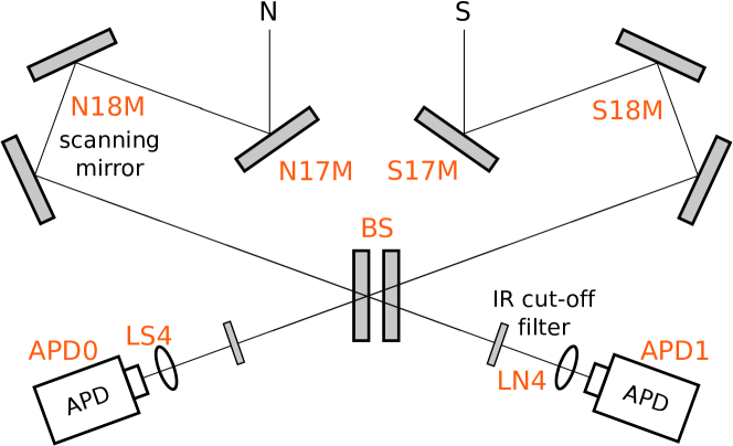
Figure 5: Schematic diagram of the MUSCA beam combiner at SUSI. The beamsplitter in the diagram is labeled BS while the APDs are single pixel avalanche photodiodes used for photon-counting.

Table 3: Specification of MUSCA

Parameter	Notation	Typical values
Spectral range ($\mu$m-1)	$\boldsymbol{\sigma}$	1/1.0 – 1/0.77
Scan range ($\mu$m)	$L_{\rm{SCAN}}$	30, 140
Number of steps per scan	$N_{\rm{STEP}}$	256, 1024
Time interval between steps (ms)	$t_{\rm{STEP}}$	0.3

4.1 Input and output of the simulator

The format of the input to the MUSCA simulator is exactly the same as the input to the PAVO simulator. Some input parameters are common to both simulators but there are some parameters which are applicable only to the MUSCA simulator. The parameters are listed in Table 1.

Instead of FITS, however, the output of the MUSCA simulator is a plain text file, which has the same format as one generated by the actual beam combiner. The file contains a time series of photon counts recorded by the APDs in the image plane as the scanning mirror periodically scans through a predetermined scan range. Each photon count has a timestamp with a precision of 10 microseconds. Fig. 6 shows an example of the photon counts recorded by the actual instrument as well as a set generated by the simulator.

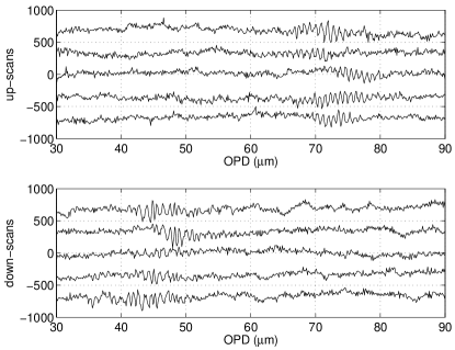
(a)

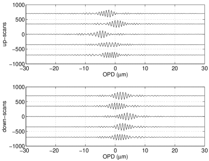
(b)

Figure 6: An example of two sets of time series of photon counts (a) recorded by the actual MUSCA beam combiner and (b) generated by the simulator plotted as separate scans. Each scan is plotted with an offset for visualization. The $x$-axis shows the relative OPD within the scan range of the scanning mirror. The top and bottom plots are scans of different direction.

4.2 Model pupil

The model of a pupil in MUSCA is straightforward as there is no spatial filter in MUSCA. Suppose the model pupil is represented again by the matrix $\mathbf{P}$ of size $N_{\rm{FFT}}\times N_{\rm{FFT}}$, then,

$$\begin{split}\mathbf{P}&=\bigcirc\circ\tilde{\mathbf{P}}\\ \end{split}$$ (21)

where $\tilde{\mathbf{P}}$ and $\bigcirc$ are defined earlier in Eq. (1) and Eq. (3) respectively.

4.3 Simulating the photon counts in a scan

The temporal fringes in MUSCA are generated using a pair of pupils, $\mathbf{P}^{(1)}$ and $\mathbf{P}^{(2)}$. In the physical instrument the pupils are aligned and combined coaxially at a beamsplitter to produce two sets of output pupils. In the simulator the output pupils are modeled as two $N_{\sigma}\times N_{\rm{STEP}}$ matrices,

$$\begin{split}\mathbf{F}^{(L)}=1+2a_{1}a_{2}\Re\left\{((\mathbf{w}\cdot\mathbf{v})^{\mathbf{T}}\mathbf{J_{1,N_{\rm{STEP}}}})\circ\mathbf{Q}\circ\exp\left(i\mathbf{\Phi}\right)\right\}\\ \mathbf{F}^{(R)}=1-2a_{1}a_{2}\Re\left\{((\mathbf{w}\cdot\mathbf{v})^{\mathbf{T}}\mathbf{J_{1,N_{\rm{STEP}}}})\circ\mathbf{Q}\circ\exp\left(i\mathbf{\Phi}\right)\right\}\end{split}$$ (22)

The matrices and their superscripts $(L)$ and $(R)$ represent the intensity of the output pupil on the left and right side of the beamsplitter. The variables $a_{1}$, $a_{2}$ and $\mathbf{w}$ are previously defined in Eq. (10) and Eq. (11). The vector $\mathbf{v}$, which is similar to the matrix $\mathbf{V}$ in Eq. (12), is the model fringe visibility of the source for the baseline defined by telescopes of pupil $\mathbf{P}^{(1)}$ and $\mathbf{P}^{(2)}$.

$$\begin{split}\mathbf{v}&=\begin{bmatrix}V(\sigma_{1}B_{1,2})&V(\sigma_{2}B_{1,2})&\cdots&V(\sigma_{N_{\sigma}}B_{1,2})\end{bmatrix}\\ \end{split}$$ (23)

Each element of $\mathbf{Q}$ is,

$$\begin{split}Q_{j,k}&=\frac{\sum_{u=1}^{N_{\rm{FFT}}}\sum_{v=1}^{N_{\rm{FFT}}}P_{u,v}^{(1,j,k)}\overline{P_{u,v}^{(2,j,k)}}}{\text{Area of circular aperture in }\bigcirc}\\ \end{split}$$ (24)

The real part of Eq. (24), $\Re\left\{Q_{j,k}\right\}$, represents the normalized intensity at wavenumber $\sigma_{j}$ due to the sum of pupils $\mathbf{P}^{(1)}$ and $\mathbf{P}^{(2)}$ at $k$-th step of a scan. $\mathbf{\Phi}$ is the additional phase difference between two telescope pupils at various wavelengths,

$$\begin{split}\mathbf{\Phi}&=2\pi\left(\boldsymbol{\sigma}\mathbf{{}^{T}}\boldsymbol{\zeta}+\mathbf{J_{N,1}}\boldsymbol{\sigma}\mathbf{NZ}+\boldsymbol{\sigma}\mathbf{{}^{T}}\mathbf{d}\right)\end{split}$$ (25)

and it is used to model the difference in piston between the pupils at each step of a scan.

The structure of Eq. (25) is very similar to Eq. (13). The first term in Eq. (25), $\boldsymbol{\zeta}$, is the astrometric OPD per scan of the baseline $\mathbf{B}_{1,2}$. Each element, $\zeta_{k}$, is evaluated at time $t_{\alpha,k}$,

$$\begin{split}\zeta_{k}&=\left|\hat{s}\cdot\mathbf{B}_{1,2}\right|_{t={t_{\alpha,k}}}\end{split}$$ (26)

where,

$$\begin{split}t_{\alpha,k}=t_{\rm{START}}+t_{\rm{STEP}}\left(\alpha N_{\rm{STEP}}+k\right)\end{split}$$ (27)

and $\alpha$ is the number of elapsed scans before the current one and $k$ is the index of a step within a scan. The typical value of $t_{\rm{STEP}}$ for MUSCA is 0.3ms. The second term in Eq. (25), $\mathbf{NZ}$, is the optical path of the delay line used to compensate the astrometric OPD. The matrix, $\mathbf{N}$, previously defined in Eq. (15), denotes the refractive indices of each optical medium in the path while the matrix, $\mathbf{Z}$, denotes the path length of each medium at every step in a scan.

$$\begin{split}\mathbf{Z}&=\begin{bmatrix}z_{1}(t_{\alpha,1})&z_{1}(t_{\alpha,2})&\cdots&z_{1}(t_{\alpha,N_{\rm{STEP}}})\\ z_{2}(t_{\alpha,1})&z_{2}(t_{\alpha,2})&\cdots&z_{2}(t_{\alpha,N_{\rm{STEP}}})\\ \vdots&\vdots&\ddots&\vdots\\ z_{N_{\rm{MED}}}(t_{\alpha,1})&z_{N_{\rm{MED}}}(t_{\alpha,2})&\cdots&z_{N_{\rm{MED}}}(t_{\alpha,N_{\rm{STEP}}})\\ \end{bmatrix}+\begin{bmatrix}\boldsymbol{\ell}\\ \mathbf{0_{1,N_{\rm{STEP}}}}\\ \vdots\\ \mathbf{0_{1,N_{\rm{STEP}}}}\\ \end{bmatrix}\end{split}$$ (28)

The values of elements in the first term of the RHS of Eq. (28) are calculated using the method described by Tango (1990). The vector $\boldsymbol{\ell}$ in Eq. (28) describes the relative change in the optical path length of air at every step in a scan due to the motion of the scanning mirror.

$$\begin{split}\boldsymbol{\ell}=&\frac{L_{\rm{SCAN}}}{N_{\rm{STEP}}-1}\times\\ &\begin{bmatrix}-N_{\rm{STEP}}/2&-N_{\rm{STEP}}/2+1&\cdots&-1&0&1&\cdots&N_{\rm{STEP}}/2-1\end{bmatrix}\\ \end{split}$$ (29)

Elements in the same column of $\mathbf{Z}$ have the same timestamp as an element with the same index in $\boldsymbol{\zeta}$. The last term in Eq. (25), $\mathbf{d}$, is the user-specified offset at each step to simulate a non-optimally compensated astrometric OPD.

$$\begin{split}\mathbf{d}&=\begin{bmatrix}d_{1}&d_{2}&\cdots&d_{N_{\rm{STEP}}}\end{bmatrix}\end{split}$$ (30)

After the pupils are combined and have formed fringes, it is assumed that the entire image of the pupil falls within the active area of the photodiodes and all photons are detected. The photodetectors in MUSCA have only one pixel and are unable to resolve any spatial variation in intensity at the image plane. Therefore only an average intensity is recorded, hence the term $\mathbf{Q}$ in Eq. (22). In addition to that the photodetectors in MUSCA are unable to resolve intensity variation across wavelengths. Therefore the number of photon counts recorded by the photodetectors is the sum of photons across the entire MUSCA operating bandwidth,

$$\begin{split}\boldsymbol{\mathcal{F}}&=N_{\rm{PHOTONS}}\times\mathbf{J_{1,N_{\sigma}}}\mathbf{F}+\boldsymbol{\epsilon}\\ \end{split}$$ (31)

Similar to Eq. (18), $N_{\rm{PHOTONS}}$ is a scaling factor that converts the intensity of the output pupil to the number of photons expected from the source given its brightness in magnitude scale and $\boldsymbol{\epsilon}$ is a noise term included to simulate photon noise and the dark count noise of the detector.

5 Converting magnitude scale to photon rate

The scaling factor $N_{\rm{PHOTONS}}$ in Section 3 and Section 4 is estimated based on the expected throughput of the beam combiner to be simulated, the efficiency (Q.E.) of the APDs and a calibrated magnitude-to-flux scaling factor, $F_{\nu}$, by Bessell (1979). The first two factors collectively describe the efficiency of the instrument, $\eta$, which is found to be $\sim$3% for PAVO and $\sim$1% for MUSCA. The lower efficiency in MUSCA is possibly due to the aluminium coated mirrors used in SUSI and a silvered beamsplitter in MUSCA. The values of $F_{\nu}$ at different photometric bands are listed in Table 4, which is reproduced from Bessell (1979). From $F_{\nu}$, the number of photons from a $m_{V}$ magnitude star collected by a telescope with an area of $A_{\rm{tel}}$ m² in $\Delta t$ seconds can be estimated. Putting the factors together,

$$\begin{split}N_{\rm{PHOTONS}}\simeq\;&\eta\times 1.51\times 10^{10}\times 10^{-m_{V}/2.5}\times F_{\nu}\frac{\Delta(1/\sigma)}{\Delta\lambda}A_{tel}\Delta t\end{split}$$ (32)

where the $\Delta(1/\sigma)$ is the bandwidth of the beam combiner and $\Delta\lambda$ is the bandwidth referred from Table 4 which has an effective wavelength close to that of the beam combiner. As an example, in the case of the MUSCA beam combiner, $\Delta(1/\sigma)\simeq 0.29\mu$m, $\Delta\lambda=0.15\mu$m, $\lambda_{\rm{eff}}=0.79$, $A_{\rm{tel}}=7\times 10^{-3}$m² and $\Delta t\simeq 80$ms (256$\times$0.3ms).

Table 4: Absolute flux calibration of $\alpha$ Lyrae (Bessell, 1979)

Filter	$\lambda_{\rm{eff}}$	$\Delta\lambda$	Flux density, $F_{\nu}$
band	($\mu$m)	($\mu$m)	($\times 10^{-23}$ W m-2 Hz-1)
U	0.36	0.076∗	1.81
B	0.44	0.094∗	4.26
V	0.55	0.088∗	3.64
R${}_{\text{C}}$	0.64	0.57-0.72	3.08
I${}_{\text{C}}$	0.79	0.725-0.875	2.55
∗http://www.astro.umd.edu/~ssm/ASTR620/mags.html

6 Simulating the effect of turbulent atmosphere

A turbulent atmosphere introduces amplitude and phase fluctuation to an otherwise plane wavefront of light from a distant star. Although amplitude fluctuation can be simulated, both PAVO and MUSCA simulators make the assumption that the atmospheric phase fluctuation only gives rise to perturbation in the phase of a wavefront. This approximation by discarding the amplitude (scintillation) term, also known as the near-field approximation, holds very well for pupils larger than 2.5cm under typical turbulence condition (Roddier, 1981).

The phase fluctuation in the atmosphere is simulated using a large ($N_{\rm{ATM}}\times N_{\rm{ATM}}$) two-dimensional array of random phasor, $\boldsymbol{\phi}$, which has a power spectrum given by (Roddier, 1981; Glindemann, 2011),

$$\begin{split}\left|\hat{\phi}_{u,v}\right|^{2}&=C\left(L_{0}^{-2}+(u^{2}+v^{2})\right)^{-11/6}\end{split}$$ (33)

The notation $\hat{\phi}$ denotes the Fourier transform of $\phi$, $u$ and $v$ are the indices of the array and $L_{0}$ is the outer scale of the turbulent structure of the model atmosphere, which is set to a very large number in the simulation. The phase fluctuation is recovered by taking the inverse Fourier transform of $\left|\hat{\phi}_{u,v}\right|\exp(i\varepsilon)$ where $\varepsilon$ is the phase of the Fourier transform and it is a random variable. The randomness of the generated phase fluctuation, $\phi$, is controlled by adjusting the scaling factor, $C$. It is tweaked so that the structure function of $\phi$,

$$\langle\left|\phi_{u,v}-\phi_{u+r_{u},v+r_{v}}\right|^{2}\rangle=6.88\left(\frac{\sqrt{r_{u}^{2}+r_{v}^{2}}}{r_{0}}\right)^{5/3}$$ (34)

has its characteristic Fried parameter, $r_{0}$, set to the value specified by the user. Fig. 7(a) shows an image of the random phases generated using this method. The grayscale of the images indicate the value of the phases.

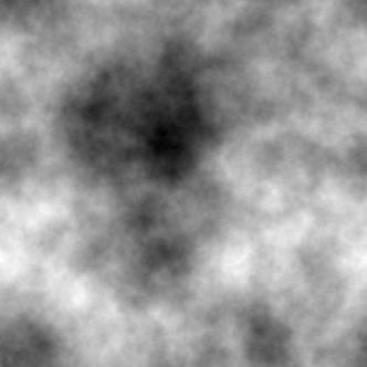
(a)

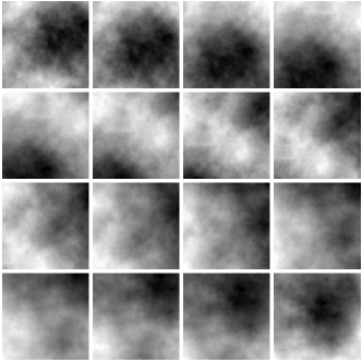
(b)

Figure 7: (a) An array of random phases generated with the inverse Fourier transform method. The value of the phases is indicated by the shades of gray in the images. (b) Small portions of the larger array in (a) sampled at slightly different positions at each time step showing the progress through time. Time increases from left to right and top to bottom.

On the other hand the phase fluctuation of a wavefront across a telescope, or $\boldsymbol{\varphi}$ in Eq. (1) and Eq. (21), is simulated by extracting a small portion ($\sim$100$\times$100) of the much larger $\boldsymbol{\phi}$ array. The typical size of the $\boldsymbol{\phi}$ array is 2048$\times$2048. Since $r_{0}$ is specified at a certain wavelength, $\sigma_{r_{0}}^{-1}$, and the phase fluctuation in $\boldsymbol{\phi}$ is generated according to $r_{0}$, the value extracted from the larger array must be scaled by a factor of $\sigma_{j}/\sigma_{r_{0}}$, where $\sigma_{j}$ is the desired wavenumber for simulation, before applying it to the model pupils in Eq. (1) and Eq. (21). The position of this small sampling window is displaced across the larger array after every time step of the simulation. This simulates the effect of Taylor’s (1938) hypothesis of a frozen atmosphere drifting across the aperture of the telescope. The rate of displacement of the sampling window depends on the wind speed which is estimated from,

$$\bar{v}=0.314\frac{r_{0}}{\tau_{0}}$$ (35)

where $\tau_{0}$ is the coherence time of the phase fluctuation and the time step of the simulation, $t_{\rm{STEP}}$. Both parameters are specified by the user. The direction of the displacement is random but remains constant throughout the simulation. Fig. 7(b) shows several snapshots of phase variation over a small portion of a larger array drifting across the sampling window.

A separate array of $\boldsymbol{\phi}$ is generated for each telescope. By doing this, it is assumed that the phase fluctuations over individual telescopes are uncorrelated. As an effect, the low-frequency phase fluctuations do not increase with baseline in the simulation. In practice this scenario is true if the baseline is longer than the outer scale of turbulence, $L_{0}$, which is in the order of 100m in the troposphere (Roddier, 1981). Therefore this approach of having a separate array of $\boldsymbol{\phi}$ for each telescope does not simulate the piston term of an aberrated pupil due to atmospheric turbulence realistically. In order to address this shortcoming in the PAVO and MUSCA simulator, the input variable, $\mathbf{D}$ or $\mathbf{d}$ (refer Table 1), can be used to add an extra differential piston between pupils from two apertures.

Another shortcoming of this method in simulating the phase variation across a turbulent atmosphere is a structure function that deviates from its theoretical value at large distances. Fig. 8 shows comparison between a theoretical structure function and one calculated from the $\boldsymbol{\phi}$. The plots in the figure are $(D_{\phi}/6.88)^{3/5}$ versus $r$ and normalized to the size of the array, $N_{\rm{ATM}}$. The theoretical Kolmogorov (KM) model curve is a straight line with unity slope ($r_{0}=1$). The deviation from the theoretical value is very pronounced especially at large distances. This is not surprising because the power spectrum, $|\hat{\phi}|^{2}$, is undersampled at low frequencies, where most of the energy resides. A practical solution to this problem, which is the approach implemented in this work, is to sub-sample the phase fluctuation from a much larger array (McGlamery, 1976; Shaklan, 1989; Lane et al, 1992). With a telescope aperture model of $\sim$5% of the size of the larger phase array, such approximation produces phase fluctuation that is at most 20% off the theoretical KM model. This is shown in Fig. 8. Also shown in the figure is a theoretical von Karman (VK) model which has a structure function very similar to that of the generated phase fluctuation. The outer scale of turbulence of the model is $\sim$44% of $N_{\rm{ATM}}$ and at this outer scale of turbulence, given the telescope aperture used in the simulation model, the variance of the tip-tilt angle of an image formed with the phase fluctuation is reduced by $\sim$40% from its expected value based on a KM model which has an infinite outer scale (Sasiela and Shelton, 1993). This reduction in tip-tilt fluctuation simulates the active tip-tilt correction at SUSI which stabilizes the image of a star.

Figure 8: Plots of $(D_{\phi}/6.88)^{3/5}$ against $r$ where $D_{\phi}$ is either a theoretical, based on a Kolmogorov (KM) model, Eq. (34), or a von Karman (VK) model (Valley, 1979)), and a simulated structure function. Both axes are normalized to the size of the random phases array. The dashed lines in the plots are the difference between the solid (KM) and dash dot (simulation) lines relative to the former. If the simulated structure function is exactly the same as the theoretical structure function then the dash lines will be horizontal at 0. The right plot is the zoomed in version of the left.

7 Testcases

The main objective of this simulation framework is to test the data reduction pipeline of the beam combiners. It is also a good tool to investigate software bugs in a data reduction pipeline during its development stage. The following sections discuss some testcases using the simulators.

Several testcases were carried out to demonstrate the functionality of the simulator and at the same time the accuracy of the data reduction pipeline for both PAVO and MUSCA. Testcase I is carried out to verify the extraction of visibility squared, $V^{2}$, of a set of fringes by the PAVO pipeline. Testcase II-IV were carried out to probe the lower bound phase error of the phase-referenced fringes constructed by the PAVO and MUSCA phase-referencing pipeline. On top of that they are also used to verify the PAVO $V^{2}$ pipeline. Table 5 shows the input for each testcase. All input parameters for Testcase II-IV are kept the same except for the fringe visibility parameter.

Table 5: Input parameters for all testcases

Testcases $\rightarrow$	I	II	III	IV
Names $\downarrow$
Section	Section 7.1	Section 7.1 & 7.2
$t_{\rm{START}}$	2455848.5
$t_{\rm{STEP}}$	PAVO: 5.0ms
	MUSCA: 0.2ms
$N_{\rm{S-FITS}}$	150
$N_{\rm{R-FITS}}$	20
$N_{\rm{F-FITS}}$	20
$N_{\rm{D-FITS}}$	20
$N_{\rm{STEP}}$	–	1024
$N_{\rm{SCAN}}$	–	150
$L_{\rm{SCAN}}$	–	140$\mu$m
$N_{\rm{MED}}$	3 (air, BK7, F7)
$\boldsymbol{\zeta}$	See Fig. 9
$N_{\rm{TEL}}$	2 (N3, S1)
$\mathbf{B}$	$|B_{1,2}|\sim$15m
$m_{V}$	Sub-case A: 0.0
	Sub-case B: 2.0
	Sub-case C: 4.0
$\mathbf{V}^{2}$	0.01–0.36	0.25	0.10	0.01
$\mathbf{D},\mathbf{d}$	See Fig. 9
$r_{0}$	10cm
$\sigma_{r_{0}}^{-1}$	0.5$\mu$m
$\tau_{0}$	1ms
$L_{0}$	100m

7.1 To verify the PAVO $V^{2}$ reduction pipeline

Testcase I-IV are used to verify the $V^{2}$ reduction pipeline of PAVO at SUSI. In these testcases the PAVO simulator is used to investigate the pipeline’s ability to reproduce the square of the visibility of a given model. The input fringe visibility for Testcase I is a sinusoidal function which models a binary star system with the primary and secondary stars almost equal in brightness (contrast ratio of $\sim$0.95) and have a projected separation of $\sim$0.04^′′ using a 15m baseline. On the other hand, the input fringe visibilities for Testcase II-IV are constant to model an unresolved single star but have different values of instrument visibilities. Since PAVO at SUSI uses only two telescopes at any one time, $\boldsymbol{\zeta}$ and $\mathbf{D}$ each reduces to a $2\times 2$ square matrix. The values of off-diagonal elements of the matrices, $\zeta_{1,2}$ and $d_{1,2}$, are shown in Fig. 9. All testcases have 3 sub-cases (A, B and C) where the photon rate is varied to simulate an observation of a zeroth, 2nd or 4th magnitude star. The number of photons in a generated PAVO frame is adjusted to match the number in an actual frame recorded by the PAVO camera at a gain of 5, for a star of magnitude $m_{V}=0.0$ and $m_{V}=2.0$, and 25, for a star of magnitude $m_{V}=4.0$.

Figure 9: The value of $\zeta_{1,2}$ and $d_{1,2}$ used in the simulation versus the frame number. The latter is a pseudo-random variable where the difference in value between each step is $d_{1,2}(t_{\alpha})-d_{1,2}(t_{\alpha-1})\sim\mathcal{N}(0,0.01)\mu$m.

The four types of frames generated by the PAVO simulator are similar to those shown in Fig. 4(c) and therefore will not be shown again in this section. The estimated $V^{2}$ of each simulated data set extracted by the PAVO pipeline are plotted against the models fed into the simulator in Fig. 10. Also plotted for comparison, in Fig. 11, are the estimated $V^{2}$ of Testcase II-IV. Both figures show that the estimated values are consistent and within 20% of the model. The expected reduction in visibility of the fringes, which is more pronounced at higher spatial frequencies (right half of the graphs), is due to the atmospheric phase noise. The observed trend in Fig. 11(b), is due to a wavelength-dependent scaling factor in the order of unity which is in turn caused by the shape of a Fourier domain windowing function used in the data reduction pipeline. This scaling factor can be calibrated out because it is identical regardless of the visibility function, as seen in Fig. 10(b) which plots the ratios between the estimated and the model $V^{2}$ (or TF) across spatial frequency. Data points with TF significantly larger than 1 is an effect of calculating a ratio with the denominator that has a very small value.

In summary, these testcases show that the $V^{2}$ reduction pipeline has some dependence on the seeing condition, which can be calibrated out, but no measurable bias as a function of target brightness and the square of the visibility of the fringes.

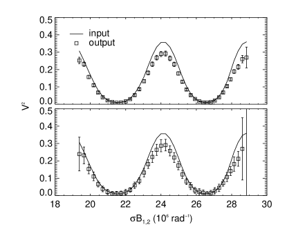
(a)

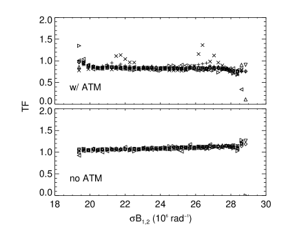
(b)

Figure 10: A comparison between user specified models of $V^{2}$ (solid line) and the estimated $V^{2}$ produced by the PAVO $V^{2}$ reduction pipeline. The top plot of (a) shows the comparison between a wavelength dependent $V^{2}$ model (input) and the (output) values estimated by the pipeline at high photon rate (sub-case A) while the bottom plot of (a) represents a similar comparison at lower photon rate (sub-case B). The ratio of estimated to model $V^{2}$ for Testcase I ($+,\times$), II ($\diamond$,$\vartriangle$), III ($\triangledown$,$\triangleright$) and IVB ($\triangleleft$) are plotted against spatial frequency in (b). Each pair of symbols in the parentheses except for Testcase IV represent sub-case A and B respectively. Also in (b), the ratios are shown when atmospheric phase noise was excluded in the simulation (no ATM).

(a)

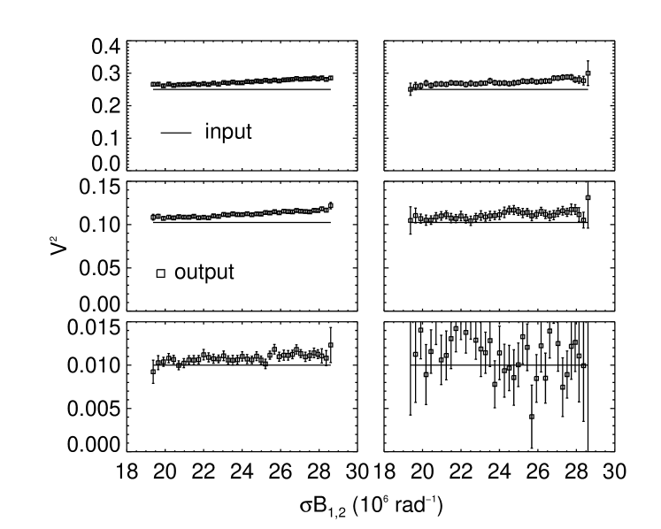
(b)

Figure 11: Similar to Fig. 10(a), the top, middle and bottom plots of (a) and (b) show the comparison between a constant $V^{2}$ model (input) and the estimated (output) of the pipeline for Testcase II, III and IV respectively. The plots on the left column are from sub-case A where the photon rate is higher than sub-case B which plots are on the right column. The estimated $V^{2}$ values of sub-case B of Testcase IV are very noise but are still unbiased. The plots in (a) are simulated with the presence of atmospheric phase noise while plots in (b) are simulated without.

7.2 To verify the PAVO and MUSCA phase-referencing pipeline

In addition to the goal mentioned in previous section, the main aim of Testcase II-IV is to test a newly written PAVO and MUSCA phase-referencing pipeline and to probe the lower bound phase error of the phase-referenced fringes. Both simulators are fed with the same input for this purpose. Some inputs which are common to both simulators, e.g. $\boldsymbol{\zeta}$ and $\mathbf{D}$ for PAVO, are resampled at a different rate for MUSCA because the time steps of the two simulators are different. Inputs which are not common to both inputs, e.g. are defined separately.

The role of the PAVO data reduction pipeline in these testcases is to provide estimates of the group and phase delay of the fringes. The group delay of the fringes is defined by the user-specified input variables, $\mathbf{D}$ and $\mathbf{d}$. The errors of the group delay estimates are shown in Fig. 12. The standard deviation of the error of the group delay estimates increases as the visibility of the fringes and the photon rate decrease. This is expected as the signal becomes weaker than the photon noise and read noise of the camera. Since the phase delay of the fringes is estimated from the group delay estimate, residuals of group delay errors which are larger than one wavelength of the fringes produce unreliable phase delay estimates. Only reliable estimates of phase delay are chosen and applied to stabilize the position of a fringe packet generated by the MUSCA simulator (Kok et al, 2012). The percentage of reliable estimates within an observation is a function atmospheric seeing, brightness of the target star and the visibility of the stellar fringes.

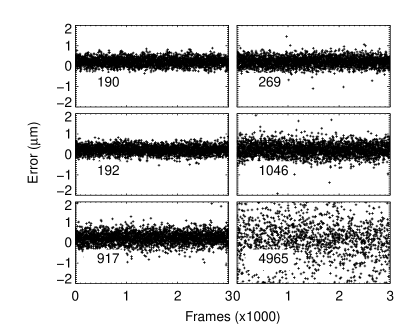
(a)

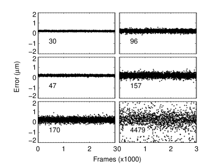
(b)

Figure 12: The errors of group delay estimates obtained from the PAVO reduction pipeline for Testcase II-IV (from top to bottom). The left and right columns are errors for sub-cases A and B respectively. The standard deviation of the errors, in unit of nanometers, are stated in the plots. The data for the plots in (a) and (b) are obtained with and without atmospheric phase noise in the simulations.

Waterfall plots in Fig. 13 show the position of the fringe packet through time. They clearly show that the fringe packet has a continuously changing position and a relatively constant position before and after the phase delay estimates are applied. The phase variation of the phase-referenced fringes across multiple scans, as seen in the plot, can be estimated from the $\langle|C|^{2}\rangle$ metric, which is a measure of the coherence of the fringes (Kok et al, 2012), and is given as,

$$\begin{split}s_{x}^{2}&\approx-2\ln{\langle|C^{2}|\rangle}\frac{N_{\rm{SC}}}{N_{\rm{SC}}-1}\left(\frac{1}{2\pi\tilde{\sigma}_{\rm{M}}}\right)^{2}\end{split}$$ (36)

where $N_{\rm{SC}}$ is the number of good scans used in the estimation and $\tilde{\sigma}_{\rm{M}}$ is the mean wavenumber of MUSCA fringes, which has a typical value of 1.2$\mu$m^-1. The factor $\frac{N_{\rm{SC}}}{N_{\rm{SC}}-1}$ is used to obtain an unbiased estimate of the sample variance. Table 6 shows the value of $\langle|C|^{2}\rangle$, $N_{\rm{SC}}$ and $s_{x}$ for all testcases.

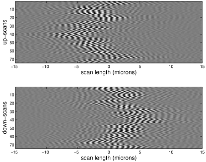
(a)

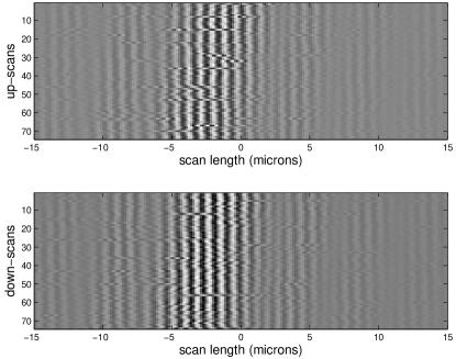
(b)

Figure 13: Simulated MUSCA fringes in a waterfall plot format showing the effect of (a) without and (b) with phase-referencing. The vertical axis is time and the horizontal axis is the optical delay. The top and bottom plots are of different scan direction.

Table 6: Results from PAVO and MUSCA phase-referencing algorithm

		with ATM			without ATM
Testcases $\downarrow$	$m_{V}$ $\rightarrow$	0.0	2.0	4.0	0.0	2.0	4.0
II ($V^{2}=0.25$)	$N_{\rm{SC}}$	74	74	72	74	74	74
	$\langle|C|^{2}\rangle$	0.6407	0.3740	0.4112	0.8236	0.5678	0.5067
	$s_{x}$ (nm)	126	188	179	84	143	156
III ($V^{2}=0.10$)	$N_{\rm{SC}}$	74	58	21	74	74	74
	$\langle|C|^{2}\rangle$	0.6387	0.2630	0.1352	0.7582	0.3752	0.3708
	$s_{x}$ (nm)	127	220	275	100	188	189
IV ($V^{2}=0.01$)	$N_{\rm{SC}}$	58	0	0	74	0	0
	$\langle|C|^{2}\rangle$	0.2684	N/A	N/A	0.3346	N/A	N/A
	$s_{x}$ (nm)	218	N/A	N/A	198	N/A	N/A

For a scan to be considered good, there must be a continuously reliable phase delay estimate throughout at least $\frac{3}{4}$ of the time to make the scan. The number of good scans as well as the value of $\langle|C|^{2}\rangle$ decrease in the same trend as the standard deviation of the errors of the group delay estimates increases because residuals of the errors which are larger than one wavelength of the fringes produce unreliable phase delay estimates. Testcase IVB is an example of an extreme case as there are no good scans found.

The summation of the phase-referenced fringes in all good scans reproduces the fringe packet without the distortion introduced by the atmospheric phase noise. The effect of coherent summation of the fringes is shown in Fig. 14. The position of the fringe packet within the scan range of the scanning mirror can be determined to an uncertainty defined by $s_{x}/\sqrt{N_{\rm{SC}}}$. For example, in order to determine the fringe packet position to an uncertainty of 5nm, which translates to an astrometric uncertainty of 10$\mu$as with 100m baseline, in Testcase IIIB, at least 1900 good scans are required. This number is not impractical as a period of good seeing at SUSI can produce over 1000 good scans (Kok et al, 2012) in about 10 minutes of observation (a total of 3600 scans) with $\beta$ Cru, which has a V magnitude of 1.3 and an uncalibrated $V^{2}$ range of 0.02–0.20 as measured by PAVO.

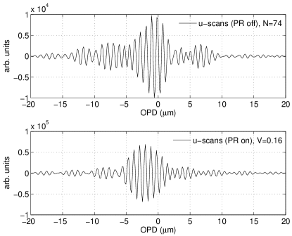
(a)

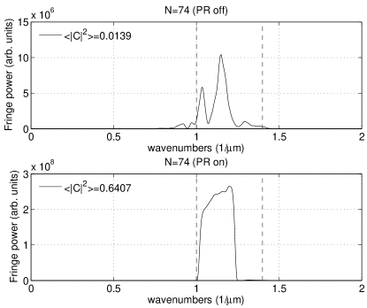
(b)

Figure 14: The top and bottom plots of (a) show the result of summation of multiple scans of incoherent and coherent fringes respectively. Similarly the top and bottom plots of (b) show the huge (about an order of magnitude) difference in the power spectrum of the incoherently and coherently summed fringe packets respectively. The number of scans used for the summation and the $\langle|C|^{2}\rangle$ metric are indicated in (b).

Although the results in Table 6 were simulated for the setup at SUSI, they can be extrapolated to estimate the performance of a similar setup at different observation sites. For example, the scenario in Testcase IIC (4th magnitude star, seeing condition of $\sim$1^′′ and diameter of light collecting aperture of 14cm) is equivalent to observing a $\sim$6th magnitude star at a site with $\sim$0.5^′′ seeing (e.g. at NPOI or in Antarctica) but with twice the aperture size (28cm). In such scenario, at least 1000 good scans are required to achieve an astrometric precision of 10$\mu$as with a 100m baseline. The phase-referencing performances in Testcase IIB and IIC are similar because a higher EMCCD gain was used to compensate the lower flux in the latter.

8 Conclusion

The simulators developed in this work not only have been a very useful tool to test the data reduction pipeline developed for the new setup and observation technique at SUSI but have also shown the feasibility of visible wavelength phase-referencing at sub-wavelength OPD uncertainty. The PAVO–MUSCA setup at SUSI can determine the position of a fringe packet of a 2-4th magnitude star to an accuracy of 5nm by coherently integrating 1000-2000 good fringe packet scans. The simulated performance of the dual beam combiner can be extrapolated to estimate performance of a similar setup at future possible sites (e.g. NPOI and Antarctica). In addition to that, due to the selection of input parameters the simulators were designed to accept they could also be used to perform simulation for many other functions (e.g. to explore the option of expanding the capability of PAVO at CHARA from a 3-telescope to a 4-telescope beam combiner or to investigate the effect of optical aberration of lenses on the performance of the beam combiners) which is beyond its main role described in this paper. The IDL code for the simulators can be obtained from the corresponding author via email.