Logarithmic correlators or responses in non-relativistic analogues of conformal invariance

Malte Henkel^a and Shahin Rouhani^b

^aGroupe de Physique Statistique, Département de Physique de la Matière et des Matériaux,

Institut Jean Lamour (CNRS UMR 7198), Université de Lorraine Nancy,

B.P. 70239, F – 54506 Vandœuvre lès Nancy Cedex, France

^b Physics Department, Sharif University of Technology, Tehran, PO Box 11165-9161, Iran

Recent developments on emergence of logarithmic terms in correlators or response functions of models which exhibit dynamical symmetries analogous to conformal invariance in not necessarily relativistic systems are reviewed. The main examples of these are logarithmic Schrödinger-invariance and logarithmic conformal Galilean invariance. Some applications of these ideas to statistical physics are described.

1 Introduction

Dynamical symmetries have become an increasingly important tool for the analysis of widely different physical systems. One particularly well-studied instance is represented by those systems admitting conformal invariance, especially in two dimensions. Conformal invariance has always been one of the central ingredients in string theory. In statistical physics, conformal invariance arises in many situations, usually for sufficiently local interactions, as a ‘natural’ extension of scale-invariance [90]. Since in two dimensions, the associated Lie algebras are infinite-dimensional, $2D$ conformal invariance furnishes particularly powerful methods for the analysis of such systems [9].

The considerable recent interest in non-relativistic analogues of the conformal algebra is on one hand motivated by studies of the AdS/CFT correspondence, in particular for topologically massive gravity [97, 36, 4, 75, 31, 104, 30] (with applications to the physics of cold atoms [25]); on the other hand by studies in the non-equilibrium statistical physics of physical ageing; or else in relationship to strongly anisotropic critical phenomena at equilibrium as exemplified by Lifshitz multicritical points. Therefore, people have considered variants of conformal transformations, where first a ‘time’-variable $t$ is distinguished with respect to the ‘space’ variables $\boldsymbol{r}$ and then a strongly anisotropic/dynamical scaling is introduced by considering the dilatations (with $\lambda=\mbox{\rm cste.}$)

$$t\mapsto\lambda^{z}t\;\;,\;\;\boldsymbol{r}\mapsto\lambda\boldsymbol{r}$$ (1.1)

such that the dynamical exponent $z$ describes the distinct behaviour of ‘time’ with respect to ‘space’.

Indeed, the list of known sets of admissible generators of space-time transformations, related to conformal transformations and which include some kind of dilatations, and which close into a Lie algebra is a rather short one. In $d+1$ space-time dimensions one has:

1. the conformal algebra $\mathfrak{conf}(d+1)$ itself, in $d+1$ dimensions, with $z=1$.

2. when considering a non-relativistic contraction

   $$t\longrightarrow t\;\;,\;\;\boldsymbol{r}\longrightarrow\boldsymbol{r}/c\;\;;\;\;c\to\infty$$ (1.2)

   one obtains the conformal Galilean algebra cga$(d)$, apparently first identified in [38], but independently rediscovered in different contexts [40, 82]. It is usually obtained, by a contraction, as the non-relativistic limit of the $(d+2)$-dimensional conformal algebra (itself obtained by a non-relativistic holographic construction) [42, 76, 2, 3, 71, 72, 61]. There is a known infinite-dimensional extension for any spatial dimension $d\geq 1$ [17]. For $d=1$, it can be constructed from a contraction of a pair of commuting Virasoro algebras [41, 44, 3]. In most representations, one has $z=1$, but representations with $z=2$ are also known [44].

3. in $d=2$ space dimensions, there exists the exotic conformal Galilean algebra ecga, which is the central extension of the non-semi-simple cga$(2)$ [74].

   Besides well-known linear equations invariant under ecga [76], invariant non-linear equations have also been found [105, 17]. All known representations have a dynamical exponent is $z=1$. See [53] for a recent review and the relationship with non-commutative mechanics.

4. The oldest known example of non-conformal space-time transformation is given by the Schrödinger algebra $\mathfrak{sch}(d)$, and was found by Jacobi in 1842/43 [59] and Lie in 1881 [73]. The known representations give a dynamical exponent $z=2$.

   Although well-known to mathematicians, physicists re-discovered it as a symmetry of free non-relativistic particles several times around 1970, including [64, 34, 83, 58]. Non-linear examples of Schrödinger-invariant equations include the Navier-Stokes equation [87, 37, 86] or Burger’s equation [84, 57].

   The Schrödinger algebra $\mathfrak{sch}(d)\subset\mathfrak{conf}(d+2)$ [11], but earlier claims that the Schrödinger algebra could be obtained by a contraction from the conformal algebra are incorrect [42].

   When classifying non-relativistic conformal Newton-Cartan space-times with a fixed dynamical exponent $z$, the two non-trivial solutions are (i) the conformal Galilei algebra cga$(d)$ for light-like geodesics and (ii) the Schrödinger algebra $\mathfrak{sch}(d)$ for time-like geodesics [23]. Remarkably, these two solutions also appeared in a search for local scale-transformations which admit the Möbius-transformations $t\mapsto(\alpha t+\beta)/(\gamma t+\delta)$ in time [41].

5. As we shall see below, the common sub-algebra $\mathfrak{age}(d)$ of both the conformal Galilean algebra cga$(d)$ and the Schrödinger algebra $\mathfrak{sch}(d)$ plays an important rôle in slow relaxation processes far from equilibrium and related to what is known in material science as ‘physical ageing’. Since physical ageing may be formally defined by its three properties of (i) slow relaxations, (ii) breaking of time-translation-invariance and (iii) dynamical scaling, the Lie algebra $\mathfrak{age}(d)$ permits more general co-variant transformations. Especially, this can be cast in the form that a non-equilibrium scaling operator should be characterised in terms of two independent scaling dimensions, denoted here $x$ and $\xi$ [89, 43]; rather than a single one as found for the Lie algebras $\mathfrak{conf}(d)$, $\mathfrak{sch}(d)$ and cga$(d)$, where $\xi=0$. This additional freedom will be seen to be important in the construction of the logarithmic extension and for the phenomenological comparison with specific models.

   Known representations of $\mathfrak{age}(d)$ in terms of local coordinates changes have either $z=2$ or $z=1$. However, when taking a coset with respect to the underlying invariant differential equation, representations for any value of $z$ are known [47, 98]. The correct geometrical interpretation of such non-local transformations is still an open question.

6. There exists for $d=1$ a closed algebra with $z=\frac{3}{2}$ [41]. It is not yet clear how this might fit into the general scheme of [23], since it does not contain the full conformal structure and furthermore its generators contain fractional space derivatives.

It is natural to wonder about the quantum realisations of these symmetries, their representations and correlation functions. Some attempts have been made at constructing NRCFT [97, 40, 93, 42, 44, 2, 3, 1, 76, 28, 23]. Many interesting features have been discovered and many questions remain. In this paper, we look at the question of whether logarithmic correlators may appear in NRCFT s analogous to their relativistic counter parts [94, 32]. Logarithmic Conformal Field Theories (LCFT s) arise when the action of the dilatation generator $L_{0}$ on primary fields is not diagonal; this may happen in some ghost theories such as the $c=-2$ theory [26]. Generically LCFT s are non unitary theories; however applications of LCFT s to some statistical models have been suggested [94, 103, 91, 33, 78, 16]. Excellent reviews of LCFT can be found within this issue. We therefore concentrate exclusively on the appearance of logarithmic conformal field theories with non relativistic symmetries (NR-LCFT).

Some examples taking from physical ageing will be used for tests and illustration.

This paper is organised as follows. Section 2 describes logarithmic Schrödinger-invariance, its descendent states and associated new invariant equations, as well as the derivation of two-point functions. In section 3, an extension towards a parabolic sub-algebra of a higher-dimensional conformal algebra is described. Physically, co-variance under this parabolic aub-algebra implies a causality condition for the $n$-point function; hence these are to be interpreted as response functions, rather than as correlators. This is important for later applications in non-equilibrium statistical physics. In section 4, the logarithmic extension of the conformal Galilean algebra are described, including also the so-called ‘exotic’ central extension in $d=2$ dimensions. Section 5 recalls briefly the context of physical ageing far from equilibrium and then describes the new features which can arise from the more general representations of the ageing algebra. Section 6 illustrates to what extent these two-point functions actually describe the non-equilibrium linear response of two paradigmatic models: (i) the $1D$ Kardar-Parisi-Zhang equation and (ii) $1D$ directed percolation (Reggeon field theory). Section 7 gives our conclusions.

2 Logarithmic Schrödinger-invariance

2.1 Lie algebra

The Schrödinger group is defined by the following set of space-time transformations

$$t\mapsto t^{\prime}=\frac{\alpha t+\beta}{\gamma t+\delta}\;\;,\;\;\boldsymbol{r}\mapsto\boldsymbol{r}^{\prime}=\frac{{\cal R}\boldsymbol{r}+\boldsymbol{v}t+\boldsymbol{a}}{\gamma t+\delta}\;\;;\;\;\alpha\delta-\beta\gamma=1$$ (2.1)

where ${\cal R}\in{\sl SO}(d)$ is a rotation matrix, $\boldsymbol{v},\boldsymbol{a}\in\mathbb{R}^{d}$ are vectors and $\alpha,\beta,\gamma,\delta$ are real numbers.

When concentrating on the changes in the coordinates $(t,\boldsymbol{r})\in\mathbb{R}_{+}\times\mathbb{R}^{d}$, one often uses the infinitesimal generators in the form (with $\partial_{i}=\partial/\partial r_{i}$)

$$P_{i} = \partial_{i}\;\;,\;\;H=-\partial_{t}\;\;,\;\;B_{i}=t\partial_{i}$$

$$J_{ij} = -\left(x_{i}\partial_{j}-x_{j}\partial_{i}\right)$$ (2.2)

$$D = -\left(2t\partial_{t}+r_{i}\partial_{i}\right)\;\;,\;\;K=-\left(tr_{i}\partial_{i}+t^{2}\partial_{t}\right)$$

which span the algebra $\mathfrak{sch}^{(0)}(d)$. Herein, the generators $P_{i},H,B_{i}$, together with the $J_{ij}$, make up the Galilei sub-algebra (still without a non-relativistic mass). The two new generators are those of dilatations ($D$) and of ‘special’ Schrödinger transformations ($K$). Lie observed that these additional space-time transformations send solutions of the free diffusion equation to other solutions [73], provided the solutions are also transformed by a further ‘companion function’ [83], see below. Furthermore, it is easy to see that the generators $H,D,K$ form a Lie algebra $\mathfrak{sl}(2,\mathbb{R})$. Finally, one has a semi-direct sum structure $\mathfrak{sch}^{(0)}(d)\cong\left(\mathfrak{sl}(2,\mathbb{R})\oplus\mathfrak{so}(d)\right)\ltimes\mathfrak{t}(2d)$, where $\mathfrak{t}(2d)$ is the $2d$-dimensional Abelian algebra generated by space translations and Galilean boosts.

One may therefore inquire whether $\mathfrak{sch}(d)$ can be extended to an infinite-dimensional Lie algebra, to be written as a semi-direct sum with one of the terms being isomorphic to a Virasoro algebra $\mathfrak{vir}$. Indeed, this can be done [39]. The resulting algebra is by now called Schrödinger-Virasoro algebra $\mathfrak{sv}(d):=\left(\mathfrak{vir}\oplus\mathfrak{so}(d)\right)\ltimes\mathfrak{hei}(d)=\left\langle X_{n},Y_{m}^{(i)},M_{n},R_{n}^{(ij)}\right\rangle_{n\in\mathbb{Z},m\in\mathbb{Z}+\frac{1}{2},i,j=1,\ldots,d}$. In $d$ spatial dimensions, the generators read [41]

$$X_{n} = -t^{n+1}\partial_{t}-\frac{n+1}{2}t^{n}r_{i}\partial_{i}-\frac{\cal M}{4}n(n+1)t^{n-1}\boldsymbol{r}^{2}-\frac{x}{2}(n+1)t^{n}$$

$$Y_{m}^{(i)} = -t^{m+\frac{1}{2}}\partial_{i}-\left(m+\frac{1}{2}\right){\cal M}t^{m-\frac{1}{2}}r_{i}$$

$$M_{n} = -t^{n}{\cal M}$$ (2.3)

$$R_{n}^{(ij)} = -t^{n}\left(r_{i}\partial_{j}-r_{j}\partial_{i}\right)$$

The Schrödinger algebra $\mathfrak{sch}(d):=\left\langle X_{\pm 1,0},Y_{\pm\frac{1}{2}}^{(i)},M_{0},R_{0}^{(ij)}\right\rangle$ is the largest finite-dimensional sub-algebra. If one sets $x=0$ and ${\cal M}=0$, then one has the following correspondence between the generators (2.2,2.3) of $\mathfrak{sch}^{(0)}(d)$:

$$Y_{-\frac{1}{2}}^{(i)}=-P_{i}\;,\;Y_{\frac{1}{2}}^{(i)}=B_{i}\;,\;X_{-1}=H\;,\;X_{0}=\frac{1}{2}D\;,\;X_{1}=K$$ (2.4)

The non-vanishing commutators of the generators (2.3) are readily obtained (with $n,n^{\prime}\in\mathbb{Z}$ and $m,m^{\prime}\in\mathbb{Z}+\frac{1}{2}$)

$$[X_{n},X_{n^{\prime}}] = (n-m)X_{n+n^{\prime}}$$

$${}[X_{n},Y_{m}^{(j)}] = \left(\frac{n}{2}-m\right)Y_{n+m}^{(j)}$$

$${}[X_{n},M_{n^{\prime}}] = -n^{\prime}M_{n+n^{\prime}}$$

$${}[X_{n},R_{n^{\prime}}^{(jk)}] = -n^{\prime}R_{n+n^{\prime}}^{(jk)}$$

$${}[Y_{m}^{(i)},Y_{m^{\prime}}^{(j)}] = \delta_{i,j}\,(m-m^{\prime})M_{m+m^{\prime}}$$ (2.5)

$${}[R_{n}^{(ij)},R_{n^{\prime}}^{(kl)}] = \delta_{i,k}R_{n+n^{\prime}}^{(jl)}+\delta_{j,l}R_{n+n^{\prime}}^{(ik)}-\delta_{i,l}R_{n+n^{\prime}}^{(jk)}-\delta_{j,k}R_{n+n^{\prime}}^{(il)}$$

$${}[R_{n}^{(ij)},Y_{m}^{(k)}] = \delta_{i,k}Y_{n+m}^{(j)}-\delta_{j,k}Y_{n+m}^{(i)}$$

The invariant free Schrödinger equation can be formally written as ${\cal S}\phi=0$, with the Schrödinger operator

$${\cal S}=2M_{0}X_{-1}-\boldsymbol{Y}_{-1/2}\cdot\boldsymbol{Y}_{-1/2}=2{\cal M}\partial_{t}-\boldsymbol{\nabla}_{\boldsymbol{r}}\cdot\boldsymbol{\nabla}_{\boldsymbol{r}}$$ (2.6)

The invariance is stated by $[{\cal S},{\cal X}]=0$ for (almost) all ${\cal X}\in\mathfrak{sch}(d)$, with the two exceptions $X_{0,1}$, where $[{\cal S},X_{0}]=-{\cal S}$ and $[{\cal S},X_{1}]=2t{\cal S}-(2x-1)M_{0}$.

It should be stressed that the generators (2.3) explicitly contain the information on the co-variant transformation of the ‘wave function’ $\phi$, which are described by (i) the scaling dimension $x$ and (ii) the non-relativistic (!) mass $\cal M$. In particular, if the scaling dimension of the wave function $x=x_{\phi}=\frac{1}{2}$, the transformations of $\mathfrak{sch}(d)$ send a solution of ${\cal S}\phi=0$ onto another solution. For a non-vanishing mass $\cal M$, two generators $Y_{m}^{(i)}$ need no longer commute. In particular, the mass generator $M_{0}$ acts as a central charge in $\mathfrak{sch}(d)$, since $[Y_{\frac{1}{2}}^{(i)},Y_{-\frac{1}{2}}^{(j)}]=\delta_{ij}M_{0}$ and hence one achieves a central extension of the abelian algebra to the Heisenberg algebra: $\mathfrak{t}(2d)\to\mathfrak{hei}(d):=\left\langle Y_{\pm\frac{1}{2}}^{(i)},M_{0}\right\rangle_{i=1,\ldots,d}$.

Since $\mathfrak{sch}(d)$ is not semi-simple, its space-time representations are all projective, as made explicit by the non-derivative terms related to $\cal M$ in the generators (2.3). True representations can be constructed [28] by first considering $\cal M$ as an additional variable and then dualising with respect to it

$$\phi(t,\boldsymbol{r})=\frac{1}{\sqrt{2\pi\,}\,}\int_{\mathbb{R}}\!{\rm d}\zeta\>\exp\left(-{\rm i}{\cal M}\zeta\right)\widehat{\phi}(\zeta,t,\boldsymbol{r})$$ (2.7)

The free Schrödinger equation becomes a Klein-Gordon equation in light-cone coordinates

$$\left(-2\partial_{\zeta}\partial_{t}+\partial_{i}\partial_{i}\right)\widehat{\phi}=0$$ (2.8)

and the metric in this space reads

$${\rm d}s^{2}=2{\rm d}\zeta{\rm d}t+{\rm d}\boldsymbol{r}\cdot{\rm d}\boldsymbol{r}$$ (2.9)

One readily rewrites the generators (2.3) in this basis. One advantage of this formulation is that the natural inclusion $\mathfrak{sch}(d)\subset\mathfrak{conf}(d+2)$ becomes obvious. In addition, this procedure suggests are further extension of the $\mathfrak{sch}(d)$ to so-called parabolic sub-algebras of $\mathfrak{conf}(d+2)$. These extensions can be used to derive causality conditions for co-variant $n$-point functions [42]. We shall describe this in section 3.

The mathematical theory of the Schrödinger-Virasoro algebra has been studied in considerable detail [93, 102].

2.2 Descendant states

In principle, there are two ways to describe infinitesimal coordinate transformation and the co-variant transformation of scaling operators $\phi$ under these. The first one is to include not only the changes of the coordinates $(t,\boldsymbol{r})$ into the generators, but also the terms describing the transformation of $\phi$ itself. This convention was applied in (2.3). Checking the Jacobi identities then automatically guarantees that the transformation of $\phi$ is consistent with the space-time transformation.

In this section, we shall follow the alternative route. The Lie algebra generators only contain the direct changes of the coordinates and one explicitly writes the transformation of the $\phi$. In the case of Schrödinger-symmetry, scaling operators are characterised by their scaling dimension $x$ and their mass $\cal M$:

$${}\left[X_{0},\phi\right]=\frac{x}{2}\phi\;\;,\;\;{}\left[M_{0},\phi\right]={\cal M}\phi$$ (2.10)

Raising (lowering) operators are $X_{n}$, $M_{n}$ and $Y_{m}^{(i)}$ with $n,m>0$ ($n,m<0$). Formally,

$${}\left[X_{0},\left[X_{n},\phi\right]\right] = \left(\frac{x}{2}-n\right)\left[X_{n},\phi\right]\;\;,\;\;$$

$${}\left[X_{0},\left[Y_{m}^{(i)},\phi\right]\right] = \left(\frac{x}{2}-m\right)\left[Y_{m}^{(i)},\phi\right]\;\;,\;\;$$ (2.11)

$${}\left[X_{0},\left[M_{n},\phi\right]\right] = \left(\frac{x}{2}-n\right)\left[M_{n},\phi\right]\;\;,\;\;$$

Since the central charge $M_{0}$ commutes with all operators, none of them can modify the value of $\cal M$.

Descendent operators will be built from the primary ones. Algebraically, a Schrödinger-primary operator $\phi$ will be characterised by being annihilated by all lowering operators

$${}\left[X_{n},\phi\right]=0\;\;,\;\;{}\left[Y_{m}^{(i)},\phi\right]=0\;\;,\;\;{}\left[M_{n},\phi\right]=0$$ (2.12)

for all $n,m>0$. In addition, using the usual operator-state correspondence, one may represent operators by states $\left|x,{\cal M}\right\rangle$. Hence, for a state with dimension $x$ and mass $\cal M$, one has

$$X_{0}\left|x,{\cal M}\right\rangle=\frac{x}{2}\left|x,{\cal M}\right\rangle\;\;,\;\;M_{0}\left|x,{\cal M}\right\rangle={\cal M}\left|x,{\cal M}\right\rangle$$ (2.13)

From now on, we shall also restrict to $d=1$ dimensions, and drop the corresponding index. Since the mass $\cal M$ cannot be modified by a raising operator, one may simplify the notation and write $\left|x,{\cal M}\right\rangle\to\left|x\right\rangle$. The effect of the raising operators is then, with $n,m<0$

$$X_{-n}\left|x\right\rangle\to\left|x+n\right\rangle\;\;,\;\;Y_{-m}\left|x\right\rangle\to\left|x+m\right\rangle\;\;,\;\;M_{-n}\left|x\right\rangle\to\left|x+n\right\rangle$$ (2.14)

The first excited state is thus $Y_{-\frac{1}{2}}\left|x\right\rangle$. The second level is obtained either by $\left(Y_{-\frac{1}{2}}\right)^{2}\left|x\right\rangle$ or by $X_{-1}\left|x\right\rangle$. However, if $x=1/2$, these two states are not independent and one rather has the first null vector

$$\left|\chi_{2}\right\rangle=\left(Y_{-\frac{1}{2}}Y_{-\frac{1}{2}}-2{\cal M}X_{-1}\right)\left|x\right\rangle$$ (2.15)

such that $\left|\chi_{2}\right\rangle=0$ gives back the Schrödinger equation (2.6). The next null state is found at level 3 for $x=\frac{11}{6}$, namely

$$\left|\chi_{3}\right\rangle=\left(3X_{-1}Y_{-\frac{1}{2}}-2Y_{-\frac{3}{2}}+\frac{3}{2{\cal M}}Y_{-\frac{1}{2}}^{3}\right)\left|x\right\rangle$$ (2.16)

Then $\left|\chi_{3}\right\rangle=0$ leads to another scale-invariant equation, namely [81]:

$$\left(3t^{2}\partial_{t}\partial_{r}-2\left(t\partial_{r}-r{\cal M}\right)-\frac{3t^{2}}{2{\cal M}}\partial_{r}^{3}\right)\phi(t,r)=0$$ (2.17)

2.3 Two-point function: non-logarithmic case

Two-point functions of primary scaling operators can be found by considering the action of the generators (2.2)

$${}\left[X_{n},\phi(t,\boldsymbol{r})\right] = \left(t^{n+1}\partial_{t}+\frac{n+1}{2}t^{n}r_{i}\partial_{i}+\frac{\cal M}{4}n(n+1)t^{n-1}\boldsymbol{r}^{2}+\frac{x}{2}(n+1)t^{n}\right)\phi(t,\boldsymbol{r})$$

$${}\left[Y_{m}^{(i)},\phi(t,\boldsymbol{r})\right] = \left(t^{m+\frac{1}{2}}\partial_{i}+\left(m+\frac{1}{2}\right){\cal M}t^{m-\frac{1}{2}}r_{i}\right)\phi(t,\boldsymbol{r})$$ (2.18)

$$\left[M_{n},\phi(t,\boldsymbol{r})\right] = t^{n}{\cal M}\phi(t,\boldsymbol{r})$$

If we had used the generators (2.3) instead, we would have simply required that $X_{n}\phi=0$ etc., with the same result.

Since the representation of $\mathfrak{sch}(d)$ under study is projective, some extra care is required for the treatment of the extra phases. Indeed, it is necessary to introduce a conjugate $\phi^{*}$ to the scaling operator $\phi$, such that $\phi^{*}$ should have the opposite mass of $\phi$, or formally

$$\left[M_{0},\phi^{*}(t,\boldsymbol{r})\right]=-{\cal M}\phi^{*}(t,\boldsymbol{r})$$ (2.19)

Requiring the co-variance under $\mathfrak{sch}(1)=\langle X_{\pm 1,0},Y_{\pm\frac{1}{2}},M_{0}\rangle$, one now looks for a two-point function of quasi-primary scaling operators

$$F=F(t_{1},t_{2};r_{1},r_{2})=\left\langle\phi_{1}(t_{1},r_{1})\phi_{2}^{*}(t_{2},r_{2})\right\rangle$$ (2.20)

If these are scalars under rotations, it is enough to consider the $1D$ case, since any two spatial points $\boldsymbol{r}_{1},\boldsymbol{r}_{2}$ can be brought to lie on a fixed line. Following [39, 46], space- and time-translation-invariance imply $F=F(t,\boldsymbol{r})$ with $t=t_{1}-t_{2}$ and $\boldsymbol{r}=\boldsymbol{r}_{1}-\boldsymbol{r}_{2}$. The requirement of Galilei-covariance leads to

$$Y_{1/2}F = \left[-t_{1}\frac{\partial}{\partial r_{1}}-{\cal M}_{1}r_{1}-t_{2}\frac{\partial}{\partial r_{2}}-(-{\cal M}_{2})r_{2}\right]F$$ (2.21)

$$= \left[\left(-t\partial_{r}-{\cal M}_{1}r\right)-r_{2}\left({\cal M}_{1}-{\cal M}_{2}\right)\right]F\>=\>0$$

This is only consistent with spatial translation-invariance if both terms in the second line vanish separately. Hence

$$\left(-t\partial_{r}-{\cal M}_{1}r\right)F = 0$$ (2.22)

$${\cal M}_{1}-{\cal M}_{2} = 0$$ (2.23)

where the first one fixes the scaling function and the second one relates the two ‘masses’ and is an example of the well-known Bargman superselection rules [6]. Next, combining dilatation-invariance with the translation-invariances gives

$$X_{0}F=\left[-t\partial_{t}-\frac{1}{2}r\partial_{r}-\frac{1}{2}(x_{1}+x_{2})\right]F=0$$ (2.24)

and finally co-variance under the special transformation gives

$$X_{1}F = \left[-t_{1}^{2}\frac{\partial}{\partial t_{1}}-t_{2}^{2}\frac{\partial}{\partial t_{2}}-t_{1}r_{1}\frac{\partial}{\partial r_{1}}-t_{2}r_{2}\frac{\partial}{\partial r_{2}}-\frac{{\cal M}_{1}}{2}r_{1}^{2}+\frac{{\cal M}_{2}}{2}r_{2}^{2}-x_{1}t_{1}-x_{2}t_{2}\right]F$$ (2.25)

$$= \left[-t^{2}\partial_{t}-tr\partial_{r}-\frac{{\cal M}_{1}}{2}r^{2}-x_{1}t\right]F(t,{r})=0$$

where both dilatation-invariance as well as both consequences of Galilei-invariance were used. In order to find $F$, multiply eq. (2.24) by $-t$ and add to eq. (2.25) and then multiply eq. (2.22) with $-r/2$ and also add. The result is the condition

$$tr(x_{1}-x_{2})F(t,r)=0$$ (2.26)

which implies that $x_{1}=x_{2}$. Using this condition, the solution of the remaining system (2.22,2.24) is elementary and gives [39], where $f_{0}$ is a normalisation constant,

$$\left\langle\phi_{1}(t_{1},\boldsymbol{r}_{1})\phi_{2}^{*}(t_{2},\boldsymbol{r}_{2})\right\rangle=\delta_{x_{1},x_{2}}\,\delta_{{\cal M}_{1},{\cal M}_{2}}\,f_{0}\,(t_{1}-t_{2})^{-x_{1}}\exp\left[-\frac{{\cal M}_{1}}{2}\frac{(\boldsymbol{r}_{1}-\boldsymbol{r}_{2})^{2}}{t_{1}-t_{2}}\right]$$ (2.27)

This is essentially the heat-kernel solution (Green’s function) of the diffusion equation. Our implicit physical convention assumes ${\cal M}_{1}>0$.

Several aspects of this result quite closely resemble the conformally invariant two-point function, especially the constraint $x_{1}=x_{2}$ on the scaling dimensions.

2.4 Two-point function: logarithmic case

The analogy of (2.27) with conformal invariance suggests that a logarithmic form might be found by assuming a logarithmic structure for the quasi-primary operators. This means that the scaling dimensions should be taken in a Jordan form (we restrict to the most simple case of rank 2). Hence there is a pair $(\phi,\psi)$ of primary operators which form a reducible, but indecomposable representation

$$X_{0}\phi(z)\left|0\right\rangle = \frac{x}{2}\phi(z)\left|0\right\rangle$$

$$X_{0}\psi(z)\left|0\right\rangle = \frac{x}{2}\psi(z)\left|0\right\rangle+\phi(z)\left|0\right\rangle$$ (2.28)

Two-point functions are now to be formed from the operators $\phi$ and $\psi$. By the same procedure as in the above subsection, we find a set of coupled differential equations for the three possible two-point functions, with the solutions

$$\left\langle\phi_{1}(t_{1},r_{1})\phi_{2}^{*}(t_{2},r_{2})\right\rangle = 0$$

$$\left\langle\phi_{1}(t_{1},r_{1})\psi_{2}^{*}(t_{2},r_{2})\right\rangle = \delta_{x_{1},x_{2}}\delta_{{\cal M}_{1},{\cal M}_{2}}t^{-x_{1}}\exp\left[-\frac{{\cal M}_{1}}{2}\frac{r^{2}}{t}\right]b$$ (2.29)

$$\left\langle\psi_{1}(t_{1},r_{1})\psi_{2}^{*}(t_{2},r_{2})\right\rangle = \delta_{x_{1},x_{2}}\delta_{{\cal M}_{1},{\cal M}_{2}}t^{-x_{1}}\exp\left[-\frac{{\cal M}_{1}}{2}\frac{r^{2}}{t}\right]\left(c-b\ln t\right)$$

with $t=t_{1}-t_{2}$ and $r=r_{1}-r_{2}$ and where $b,c$ are free normalisation constants.

Alternatively, one may also work with nilpotent variables

$$\theta^{2}=0$$ (2.30)

We then assume the existence of quasi-primary operators and states [80]

$$\Phi(z,\theta) = \phi(z)+\theta\psi(z)$$

$$\Phi(z,\theta)\left|0\right\rangle = \left|x/2+\theta\right\rangle$$ (2.31)

$$X_{0}\left|x/2+\theta\right\rangle = (x/2+\theta)\left|x/2+\theta\right\rangle$$

and we define the two-point function as

$$\left\langle\Phi_{1}(t_{1},r_{1},\theta_{1})\Phi_{2}^{*}(t_{2},r_{2},\bar{\theta}_{2})\right\rangle=F(t_{1},t_{2};r_{1},r_{2};\theta_{1},\bar{\theta}_{2})$$ (2.32)

and a conjugate nilpotent variable $\bar{\theta}_{2}$ appeared in the conjugate operator $\Phi_{2}^{*}$. Requiring co-variance under the Schrödinger algebra, we find

$$F=\delta_{x_{1},x_{2}}\delta_{{\cal M}_{1},{\cal M}_{2}}t^{-x_{1}-\theta_{1}-\bar{\theta}_{2}}\exp\left[-\frac{{\cal M}_{1}}{2}\frac{r^{2}}{t}\right]\left(b\left(\theta_{1}+\bar{\theta}_{2}\right)+c\theta_{1}\bar{\theta}_{2}\right)$$ (2.33)

and after expanding, leads to

$$F=\delta_{x_{1},x_{2}}\delta_{{\cal M}_{1},{\cal M}_{2}}t^{-x_{1}}\exp\left[-\frac{{\cal M}_{1}}{2}\frac{r^{2}}{t}\right]\left(b\left(\theta_{1}+\bar{\theta}_{2}\right)+\theta_{1}\bar{\theta}_{2}\left(c-2b\ln t\right)\right)$$ (2.34)

However, we can expand the two-point function (2.32) as follows:

$$\left\langle\Phi_{1}(t_{1},r_{1},\theta_{1})\Phi_{2}^{*}(t_{2},r_{2},\bar{\theta}_{2})\right\rangle$$ (2.35)

$$= \left\langle\phi_{1}(t_{1},r_{1})\phi_{2}^{*}(t_{2},r_{2})\right\rangle+\bar{\theta}_{2}\left\langle\phi_{1}(t_{1},r_{1})\psi_{2}^{*}(t_{2},r_{2})\right\rangle$$

$$+{\theta}_{1}\left\langle\psi_{1}(t_{1},r_{1})\phi_{2}^{*}(t_{2},r_{2})\right\rangle+\theta_{1}\bar{\theta}_{2}\left\langle\psi_{1}(t_{1},r_{1})\psi_{2}^{*}(t_{2},r_{2})\right\rangle$$

Comparison with the expansion of the two-point function in (2.34) reproduces all three two-point functions in (2.29).

3 Extension to parabolic sub-algebras and implications for causality

There is a natural extension of the Schrödinger algebra which allows to derive causality properties of the co-variant $n$-point functions from purely algebraic criteria. Recall the root diagramme associated with a Lie algebra [66], for the special case $d=1$: to each generator ${\cal X}\in\mathfrak{sch}(1)$ one associates a planar vector $\stackrel{{\scriptstyle\to}}{{\boldsymbol{x}}}\in\Delta$ on a root lattice. Under this correspondence, forming the commutator $[{\cal X},{\cal X}^{\prime}]={\cal Y}$ corresponds to vector addition $\stackrel{{\scriptstyle\to}}{{\boldsymbol{x}}}+\stackrel{{\scriptstyle\to}}{{\boldsymbol{x}^{\prime}}}=\stackrel{{\scriptstyle\to}}{{\boldsymbol{y}}}$. If that vector sum $\stackrel{{\scriptstyle\to}}{{\boldsymbol{y}}}$ falls outside the lattice $\Delta$, it is understood that ${\cal Y}=0$.

    

Figure 1: Root diagrammes of some sub-algebras of the complex Lie algebra $B_{2}$. The roots of $B_{2}$ are indicated by the full and broken dots, those of the sub-algebras by the full dots only.
(a) Schrödinger algebra $\mathfrak{sch}(1)=\left\langle X_{\pm 1,0},Y_{\pm 1/2},M_{0}\right\rangle$ and the maximal parabolic sub-algebra $\widetilde{\mathfrak{sch}}(1)=\mathfrak{sch}(1)+\mathbb{C}N$.
(b) Conformal Galilean algebra $\mbox{\sc cga}(1)=\left\langle X_{\pm 1,0},Y_{\pm 1,0}\right\rangle$.

In figure 1a, this is illustrated for the Lie algebra $\mathfrak{sch}(1)$. Since it closes as a Lie algebra, the set of associated points must be convex. For example, it can be readily seen that the generator $M_{0}$ indeed is central. Furthermore, the same diagramme also illustrates the inclusion $\mathfrak{sch}(1)\subset\mathfrak{conf}(3)\cong B_{2}$, one of the well-known simple Lie algebras of rank 2 in the Cartan classification and isomorphic to the algebra of conformal transformations in 3 dimensions.

There is an intermediate step between the algebra $\mathfrak{sch}(1)$ and the full conformal algebra $\mathfrak{conf}(3)$. These are the parabolic sub-algebras (in this case of $B_{2}$). By definition [66], a parabolic sub-algebra consists of the Cartan sub-algebra $\mathfrak{h}$ and the set of all ‘positive’ roots. A root is called positive, if it is to the right of a straight line which passes through the origin of the graph, see figure 2. For $\mathfrak{sch}(1)$ this straight line rune with a slope of $45^{\circ}$ through the root diagramme of $B_{2}$, see figure 1a. With respect to $\mathfrak{sch}(1)$, the parabolic sub-algebra $\widetilde{\mathfrak{sch}}(1):=\mathfrak{sch}(1)+\mathbb{C}N$ contains an extra generator $N$. Several set of roots can be mapped onto each other by elements of the Weyl group and such pairs of sets are isomorphic as Lie algebras. Because of the Weyl symmetries, the slope $\sigma$ of the straight line can be taken to lie between $1$ and $\infty$. In figure 2, it is illustrated that there are three non-isomorphic parabolic sub-algebras of $B_{2}\cong\mathfrak{conf}(3)$. The generic case, with $1<\sigma<\infty$, is the extended ageing algebra $\widetilde{\mathfrak{age}}(1)=\mathfrak{age}(1)+\mathbb{C}N$, which we shall discuss below in section 5. If the slope $\sigma=1$, one has the extended Schrödinger algebra $\widetilde{\mathfrak{sch}}(1)$ and for a slope $\sigma=\infty$ one has the extended conformal Galilei algebra $\widetilde{\mbox{\sc cga}}(1)$. For a formal proof of this classification, see [42].

Figure 2: Classification of the parabolic sub-algebras of the simple complex algebra $B_{2}$. The generators are indicated by the full dots and the double-degenerate Cartan sub-algebra $\mathfrak{h}$. The three non-isomorphic parabolic sub-algebras of $B_{2}$ are (a) the extended Schrödinger algebra $\widetilde{\mathfrak{sch}}(1)$ (b) the extended ageing algebra $\widetilde{\mathfrak{age}}(1)$ (c) the extended conformal Galilean algebra $\widetilde{\mbox{\sc cga}}(1)$.

This extension to $\widetilde{\mathfrak{sch}}(1)$ is more easy to see in the dual variables introduced in (2.7). The representation (2.3) is rewritten as

$$X_{n} = \frac{{\rm i}}{2}(n+1)nt^{n-1}{r}^{2}\partial_{\zeta}-t^{n+1}\partial_{t}-\frac{n+1}{2}t^{n}{r}\partial_{r}-\frac{n+1}{2}xt^{n}$$

$$Y_{m} = {\rm i}\left(m+\frac{1}{2}\right)t^{m-1/2}r\partial_{\zeta}-t^{m+1/2}\partial_{j}$$

$$M_{n} = {\rm i}t^{n}\partial_{\zeta}$$ (3.1)

The extension to the maximal parabolic sub-algebra is achieved by including the generator [42]

$$N:=\zeta\partial_{\zeta}-t\partial_{t}+\xi\,.$$ (3.2)

It is well-known that co-variance under this extra generator is sufficient to derive causality conditions of the form $t>0$ for the two-point functions, and also similarly for the three-point function [42].

We wish to study the consequences for logarithmic representations, built in analogy with those of the Schrödinger algebra $\mathfrak{sch}(1)$. Formally, this will again be achieved by replacing the scaling dimension $x$ by a Jordan matrix $x\mapsto\left(\begin{array}[]{ll}x&1\\ 0&x\end{array}\right)$. The co-variant two-point functions, built from quasi-primary scaling operators $\left(\mbox{${\begin{array}[]{c}\phi_{i}\\ \psi_{i}\end{array}}$}\right)$, are

$$\widehat{F}(\zeta,t,r) := \left\langle\widehat{\phi}_{1}(\zeta_{1},t_{1},r_{1})\widehat{\phi}_{2}(\zeta_{2},t_{2},r_{2})\right\rangle$$

$$\widehat{G}_{12}(\zeta,t,r) := \left\langle\widehat{\phi}_{1}(\zeta_{1},t_{1},r_{1})\widehat{\psi}_{2}(\zeta_{2},t_{2},r_{2})\right\rangle$$

$$\widehat{G}_{21}(\zeta,t,r) := \left\langle\widehat{\psi}_{1}(\zeta_{1},t_{1},r_{1})\widehat{\phi}_{2}(\zeta_{2},t_{2},r_{2})\right\rangle$$ (3.3)

$$\widehat{H}(\zeta,t,r) := \left\langle\widehat{\psi}_{1}(\zeta_{1},t_{1},r_{1})\widehat{\psi}_{2}(\zeta_{2},t_{2},r_{2})\right\rangle$$

where $\zeta=\zeta_{1}-\zeta_{2}$, $t=t_{1}-t_{2}$ and $r=r_{1}-r_{2}$ and the three translation-symmetries are taken into account. As in logarithmic conformal invariance and analogously to the calculations in section 2, one may derive a set of linear first-order differential equations for these four two-point functions. For $\mathfrak{sch}(1)$-covariance alone, the result [49] is, subject to the additional constraint $x:=x_{1}=x_{2}$, that $\widehat{F}=0$ and

$$\widehat{G}_{12}=\widehat{G}_{21}=\widehat{G}(t,u) = |t|^{-x}\widehat{g}\left(u|t|^{-1}\right)$$

$$\widehat{H}(t,u) = |t|^{-x}\left(\widehat{h}\left(u|t|^{-1}\right)-\ln|t|\widehat{g}\left(u|t|^{-1}\right)\right)$$ (3.4)

where $u=2\zeta t+{\rm i}r^{2}$ and $\widehat{g}$ and $\widehat{h}$ are arbitrary (differentiable) functions. Backtransforming to the masses ${\cal M}_{1,2}$, one reproduces the known form (2.29).

New results can be found by requiring co-variance under the larger algebra $\widetilde{\mathfrak{sch}}(1)$. For the logarithmic case, $\xi$ should be replaced by a matrix. Furthermore, it can be shown that this matrix also must be of Jordan form [49]

$$N:=\zeta\partial_{\zeta}-t\partial_{t}+\left(\begin{array}[]{ll}\xi&\xi^{\prime}\\ 0&\xi\end{array}\right).$$ (3.5)

Co-variance under $N$ fixes the two undetermined scaling functions in (3.4), with the result

$$\widehat{G}(\zeta,t,r) = \widehat{g}_{0}\,|t|^{-x}\>\left(\frac{2\zeta t+{\rm i}r^{2}}{|t|}\right)^{-x-\xi_{1}-\xi_{2}}$$

$$\widehat{H}(\zeta,t,r) = |t|^{-x}\>\left(\frac{2\zeta t+{\rm i}r^{2}}{|t|}\right)^{-x-\xi_{1}-\xi_{2}}$$

$$\times\left(\widehat{h}_{0}+\widehat{g}_{0}(1+\xi_{1}^{\prime}+\xi_{2}^{\prime})\ln\left(\frac{2\zeta t+{\rm i}r^{2}}{|t|}\right)-\widehat{g}_{0}\,\ln|t|\right)$$

where $\widehat{g}_{0}$ and $\widehat{h}_{0}$ are normalisation constants. One may transform this back to the masses ${\cal M}_{1,2}>0$. Again, one recovers exactly the previously found forms (2.29), but now with the important extra information, that $t=t_{1}-t_{2}>0$. If that condition is not met, the two-point function vanishes [49].

Causality conditions of this kind suggest that the two-point functions just calculated are better not interpreted as two-time correlators $C(t,s)=\langle\phi(t)\phi(s)\rangle=C(s,t)$, but rather as linear response functions $R(t,s)=\left.\frac{\delta\langle\phi(t)\rangle}{\delta h(s)}\right|_{h=0}=\Theta(t-s)\widetilde{r}(t,s)$, which measures the response of an average $\langle\phi(t)\rangle$ at some time $t$ with respect to an external perturbation which naturally should have occurred at an earlier time $s<t$, as expressed by the Heaviside function $\Theta(t-s)$.

4 Logarithmic conformal Galilean algebra, including the exotic case

4.1 conformal Galilean algebra

The conformal Galilean algebra (cga) can be obtained directly by contraction from the conformal algebra [38]. Alternatively, one may also start from the so-called $l$-Galilei algebra [40] and recognise the cga as the $l=1$ special case [40, 82]. The embedding $\mbox{\sc cga}(1)\subset\mathfrak{conf}(3)\cong B_{2}$ and the associated parabolic extension is illustrated in figure 2c. This algebra is a straightforward generalisation of the transformations defined by eq. (2.1). We admit here a more general from;

$$t\mapsto t^{\prime}=\frac{\alpha t+\beta}{\gamma t+\delta}\;\;,\;\;\boldsymbol{r}\mapsto\boldsymbol{r^{\prime}}=\frac{\mathcal{R}\boldsymbol{r}+t^{2l}\boldsymbol{b}_{2l}+\cdots+\boldsymbol{b}_{1}t+\boldsymbol{b}_{0}}{\gamma t+\delta}\;\;,\;\;\alpha\delta-\beta\gamma=1.$$ (4.1)

The algebra of the symmetry operators closes only for $l\in\frac{1}{2}\mathbb{Z}$. Recall that the dynamical exponent $z=1/l$ is related to the inverse of $l$,

$$t\mapsto\lambda^{2}t,\quad\boldsymbol{r}\mapsto\lambda^{2l}\boldsymbol{r}$$ (4.2)

thus only certain non-relativistic systems are included in this scheme. The case of Schrödinger symmetry corresponds to $l=1/2$. The case of $l=1$ leads to the cga. Clearly, the dynamical exponent associated with this representation of the cga is $z=1$. In $d+1$-dimensions, in addition to the usual generators of the Galilean algebra, $\{J_{i,j},H,P_{i},B_{i}\}$ in eq. (2.2), $\mbox{\sc cga}(d)$ has $d+2$ more generators:

$$D=-(t\partial_{t}+r_{i}\partial_{i}),\qquad K=-(2tr_{i}\partial_{i}+t^{2}\partial_{t}),\qquad K_{i}=t^{2}\partial_{i}.$$ (4.3)

In contrast to the projective representations of the Schrödinger algebra, there is no analogue of a non-relativistic ‘mass’ $\cal M$. Similar to the Schrödinger algebra, the $\mbox{\sc cga}(d)$ admits an affine extension [41], often called the full cga: As in previous sections, one may include into the generators immediately also the terms which describe the co-variant transformation of the scaling operators. Then the generators of the full cga may be written as follows [17]

$$X_{n} = -t^{n+1}\partial_{t}-(n+1)t^{n}\boldsymbol{r}\cdot\boldsymbol{\nabla}_{\boldsymbol{r}}-n(n+1)t^{n-1}\boldsymbol{\gamma}\cdot\boldsymbol{r}-x(n+1)t^{n}$$

$$Y_{n}^{(j)} = -t^{n+1}\partial_{j}-(n+1)t^{n}\gamma_{j}$$ (4.4)

$$J_{n}^{(jk)} = -t^{n}\bigl{(}r_{j}\partial_{k}-r_{k}\partial_{j}\bigr{)}-t^{n}\bigl{(}\gamma_{j}\partial_{\gamma_{k}}-\gamma_{k}\partial_{\gamma_{j}}\bigr{)}$$

where $\boldsymbol{\gamma}=(\gamma_{1},\ldots,\gamma_{d})$ is a vector of dimensionful constants, $x$ is again a scaling dimension and $n\in\mathbb{Z}$. The maximal finite-dimensional sub-algebra is the cga(d), see figure 1b for a root diagramme for $d=1$. If one sets $x=0$ and $\boldsymbol{\gamma}=\boldsymbol{0}$, the correspondence with (4.3) reads:

$$X_{-1} = H\;\;,\;\;X_{0}\>=\>D\;\;,\;\;X_{1}\>=\>K,$$

$$Y_{-1}^{(i)} = -P_{i}\;\;,\;\;Y_{0}^{(i)}\>=\>-B_{i}\;\;,\;\;Y_{1}^{(i)}\>=\>-K_{i}.$$ (4.5)

The commutation relations of the full cga are (with the habitual correspondence $J_{ij}=-J_{ji}\leftrightarrow J^{(a)}$):

$$[X_{n},X_{m}] =(m-n)X_{n+m},\quad [X_{m},J_{n}^{(a)}] =-nJ_{n+m}^{(a)},$$ (4.6)

$$[J_{m}^{(a)},J_{n}^{(b)}] =-{f^{ab}}_{c}J_{n+m}^{(c)},\quad [X_{m},Y_{n}^{(i)}[ =(m-n)Y_{n+m}^{(i)},$$

$$[Y_{m}^{(i)},Y_{n}^{(j)}] =0,\quad [Y_{m}^{(i)},J_{n}^{(jk)}] =\left(Y_{n+m}^{(j)}\delta^{ik}-Y_{n+m}^{(k)}\delta^{ij}\right).$$

where ${f^{ab}}_{c}$ are the structure constants of the Lie algebra $\mathfrak{so}(d)$. The two-point functions of this algebra were first given in [41, 44] and then re-derived in [2, 1]. In the representation (4.4), they are of the form $\sim|t|^{-2x}\exp\left[-2{\boldsymbol{\gamma}\cdot\boldsymbol{r}}/t\right]$. Different representations of $\mbox{\sc cga}(1)$ and the resulting two-point functions are given in [44].

To obtain representations in $1+1$ dimensions, we first observe that the full cga in this dimension can be obtained directly from a contraction of CFT₂. To observe this contraction, we go to complex coordinates, $z=t+{\rm i}r/c$. Relativistic conformal symmetry of $d=2$ contains two copies of the Virasoro algebra:

$$L_{n}=-z^{n+1}\partial_{z},\qquad\bar{L}_{n}=-\bar{z}^{n+1}\partial_{\bar{z}},$$ (4.7)

which are the generators of holomorphic and antiholomorphic transformations. Now, we impose the contraction of eq. (1.2), and in the limit $c\to\infty$ we have the generators [54, 2]:

$$X_{n}=L_{n}+\bar{L}_{n}+\text{O}(1/c),\quad Y_{n}=-\frac{{\rm i}}{c}(L_{n}-\bar{L}_{n})+\text{O}(1/c).$$ (4.8)

A different contraction builds first a different representation of $2D$ conformal invariance (which leads to distinct two-point functions) before contracting [41, 44]. Now that we have the full cga algebra obtained from contraction of CFT₂, we might be able to obtain its representations by contraction as well. It is not always true that representations of an algebra can be obtained from contraction as well. However, in this case it is possible. The result is that the full cga in $d=1$ contains to distinct central charges $c_{1}$ and $c_{2}$ [88]:

$$[X_{m},X_{n}] =(m-n)X_{m+n}+\tfrac{1}{12}c_{1}m(m^{2}-1)\delta_{m+n,0},$$ (4.9)

$$[X_{m},Y_{n}] =(m-n)Y_{m+n}+\tfrac{1}{12}c_{2}m(m^{2}-1)\delta_{m+n,0}.$$

The independence of these two central charges $c_{1,2}$ can be seen in a simple way through the following example: consider the generators $V_{n}$ and $V_{n}^{\prime}$ ($n\in\mathbb{Z}$) of two commuting Virasoro algebras with central charges $c$ and $c^{\prime}$. Then identify

$$X_{n}\mapsto\left(\begin{array}[]{cc}V_{n}+V_{n}^{\prime}&0\\ 0&V_{n}+V_{n}^{\prime}\end{array}\right),\ Y_{n}\mapsto\left(\begin{array}[]{cc}0&V_{n}\\ 0&0\end{array}\right),\ c_{1}\mapsto(c+c^{\prime})\left(\begin{array}[]{cc}1&0\\ 0&1\end{array}\right),\ c_{2}\mapsto c^{\prime}\left(\begin{array}[]{cc}0&1\\ 0&0\end{array}\right)$$ (4.10)

Two-point functions of the full cga can as well be obtained via contraction:

$$\langle\phi_{1}(t_{1},r_{1})\phi_{2}(t_{2},r_{2})\rangle_{\text{CGA}} =\lim_{c\to\infty}\langle\phi_{1}(t_{1},r_{1})\phi_{2}(t_{2},r_{2})\rangle_{\text{CFT}}$$ (4.11)

$$=\lim_{c\to\infty}A\delta_{h_{1},h_{2}}\delta_{\bar{h}_{1},\bar{h}_{2}}(t_{12}-\tfrac{{\rm i}}{c}r_{12})^{-(x-{\rm i}c\gamma)}(t_{12}-\tfrac{i}{c}x_{12})^{-(x-{\rm i}c\gamma)}$$

$$=a\delta_{x_{1},x_{2}}\delta_{\gamma_{1},\gamma_{2}}\,t_{12}^{-2x_{1}}\exp\left[\tfrac{-2\gamma_{1}r_{12}}{t_{12}}\right].$$

with the abbreviations $t_{12}=t_{1}-t_{2}$ and $r_{12}=r-1-r_{2}$. Now, we consider the logarithmic representations and find its contracted form, for the special case $d=1$. In the logarithmic representation and taking the simplest rank two Jordan cell, we need two states $\left|x,\gamma,0\right\rangle$ and $\left|x,\gamma,1\right\rangle$. The action of the generators on the first one is conventional

$$X_{0}\left|x,\gamma,0\right\rangle =x\left|x,\gamma,0\right\rangle,$$ (4.12)

$$Y_{0}\left|x,\gamma,0\right\rangle =\gamma\left|x,\gamma,0\right\rangle.$$

whereas action on the logarithmic partner $\left|x,\gamma,1\right\rangle$ is more involved:

$$X_{0}\left|x,\gamma,1\right\rangle =x\left|x,\gamma,1\right\rangle+\left|x,\gamma,0\right\rangle$$ (4.13)

$$Y_{0}\left|x,\gamma,1\right\rangle =\gamma\left|x,\gamma,1\right\rangle.$$

So, it appears that $Y_{0}$ acts diagonally and logarithms do not involve the rapidity $\gamma$. To derive the logarithmic two-point functions, we follow the contraction approach for logarithmic two-point functions resulting in:

$$\langle\phi_{1}(t_{1},r_{1})\phi_{2}(t_{2},r_{2})\rangle_{\text{\sc CGA}} =0,$$ (4.14)

$$\langle\phi_{1}(t_{1},r_{1})\psi_{2}(t_{2},r_{2})\rangle_{\text{\sc CGA}} =\lim_{c\to\infty}\langle\phi_{1}(t_{1},r_{1})\psi_{2}(t_{2},r_{2})\rangle_{\text{CFT}}$$

$$=b\delta_{x_{1},x_{2}}\delta_{\gamma_{1},\gamma_{2}}\,t_{12}^{-2x_{1}}\exp\left[-\tfrac{2\gamma_{1}r_{12}}{t_{12}}\right].$$

For last two-point function again we have:

$$\langle\psi_{1}(t_{1},r_{1})\psi_{2}(t_{2},r_{2})\rangle_{\text{\sc CGA}} =\lim_{c\to\infty}\langle\psi_{1}(t_{1},r_{1})\psi_{2}(t_{2},r_{2})\rangle_{\text{CFT}}$$

$$=\delta_{x_{1},x_{2}}\delta_{\gamma_{1},\gamma_{2}}\,t_{12}^{-2x_{1}}\exp\left[-\tfrac{2\gamma_{1}r_{12}}{t_{12}}\right]\left(d-2b\log t_{12}\right).$$ (4.15)

All this procedure may be redone using the nilpotent variables [80], directly deriving the correlators using the non-relativistic algebra. We are also able to consider a Jordan cell structure for the rapidity:

$$X_{0}\left|x,\gamma,1\right\rangle =x\left|x,\gamma,1\right\rangle+x^{\prime}\left|x,\gamma,0\right\rangle$$ (4.16)

$$Y_{0}\left|x,\gamma,1\right\rangle =\gamma\left|x,\gamma,1\right\rangle+\gamma^{\prime}\left|x,\gamma,0\right\rangle.$$

And a simple change appears:

$$\langle\psi_{1}(t_{1},r_{1})\psi_{2}(t_{2},r_{2})\rangle=\delta_{x_{1},x_{2}}\delta_{\gamma_{1},\gamma_{2}}\,t_{12}^{-2x_{1}}\exp\left[-2\gamma_{1}\tfrac{r_{12}}{t_{12}}\right]\left(-2bx^{\prime}\log t_{12}-2a\gamma^{\prime}\tfrac{r_{12}}{t_{12}}+2d\right).$$ (4.17)

This is an interesting development suggesting that chiral LCFTs should exist.

4.2 Exotic Galilean Conformal Algebra (ecga)

The algebra $\mbox{\sc cga}(2)$ admits an extra central charge in $(2+1)$ dimensions [74]. In fact the commutator of boosts is no longer vanishing, reminiscent of non-commutative theories:

$$[B_{i},B_{j}]=\mathcal{B}\epsilon_{ij},\qquad[P_{i},K_{j}]=-2\mathcal{B}\epsilon_{ij},$$ (4.18)

where $\epsilon_{ij}$ is the antisymmetric $2$-dimensional tensor. Here $\mathcal{B}$ commutes with all generators of the algebra and is therefore an extra central charge. Its physical significance has been of interest [23]. The central charge can also be obtained by contraction and two-point function is realised using auxiliary coordinates [76]. Examples of systems of non-linear equations with the ecga as a dynamical symmetry are given in [17].

To proceed we follow [76] and introduce an auxiliary internal space with three dimensions $w$, $v_{1}$, $v_{2}$ (therefore we have a six-dimensional space now). Using these coordinates new differential operators for the generators of ecga may be written:

$$H =-\partial_{t}, D =-r_{i}\partial_{i}-t\partial_{t}-x, K =-2tr_{i}\partial_{i}-t^{2}\partial_{t}-2r_{i}\chi_{i},$$ (4.19)

$$P_{i} =-\partial_{i}, B_{i} =-t\partial_{i}-\chi_{i}, K_{i} =-t^{2}\partial_{i}+2t\chi_{i}-2r_{j}\epsilon_{ij}\gamma$$

$$J =-\epsilon_{ij}r_{j}\partial_{j}-\tfrac{1}{2\gamma}\chi_{i}\chi_{i}, \mathcal{B} =\partial_{w}, \chi_{i} =\partial_{v_{i}}-\tfrac{1}{2}\epsilon_{ij}v_{j}\partial_{w}.$$

The operator $J$ plays the role of rapidity here. In this realisation one desires local operators to be simultaneous eigenstates of $D$ and $\mathcal{B}$:

$$[D,\phi]=x\phi,\qquad[\mathcal{B},\phi]=\gamma\phi.$$ (4.20)

Now, if we look for the most general case, local fields will have to be eigenstates of $K_{i}$ as well. The two point function of ecga (without rapidity) has been worked out [76]:

$$\langle\phi_{1}(t_{1},\boldsymbol{r_{1}})\phi_{2}(t_{2},\boldsymbol{r_{2}})\rangle=\delta_{x_{1},x_{2}}\delta_{\gamma_{1}+\gamma_{2},0}\,t^{-2x_{1}}\exp\left[\tfrac{1}{2}\gamma\epsilon_{ij}(\tfrac{1}{4}v_{j}^{+}-u_{j})v_{i}\right]\,\mathcal{O}_{1}(u_{i}+\tfrac{1}{2}v_{i}^{+}),$$ (4.21)

in which $\mathcal{O}$ is an arbitrary function, $\boldsymbol{u}=(\boldsymbol{r}_{1}-\boldsymbol{r}_{2})/(t_{1}-t_{2})$ and $v^{+}=v_{1}+v_{2}$. Here, we add the explicit dependence on the ecga-rapidity

$$\langle\Phi_{1}(t_{1},\boldsymbol{r}_{1},\boldsymbol{v}_{1}) \Phi_{2}(t_{2},\boldsymbol{r}_{2},\boldsymbol{v}_{2})\rangle=$$

$$t^{-x^{+}}\exp\left[-\tfrac{1}{2}(\lambda_{i}-\tfrac{1}{4}\gamma\epsilon_{ij}v_{j}^{+}+\gamma\epsilon_{ij}u_{j})v_{i}-u_{i}\lambda_{i}^{+}\right]\,\mathcal{O}_{1}(\boldsymbol{u}-\tfrac{1}{2}\boldsymbol{v}^{+}),$$ (4.22)

where $\lambda^{+}=\lambda_{1}+\lambda_{2}$ and $x^{+}=x_{1}+x_{2}$. The function $\mathcal{O}_{1}$ now satisfies some constraints [55]. To find the logarithmic version of the two point functions one can add a nilpotent variable to the fields and after some algebra one finds:

$$\langle\Phi_{1}(t_{1},\boldsymbol{r}_{1},\boldsymbol{v}_{1})\Phi_{2}(t_{2},\boldsymbol{r}_{2},\boldsymbol{v}_{2})\rangle =0,$$ (4.23)

$$\langle\Phi_{1}(t_{1},\boldsymbol{r}_{1},\boldsymbol{v}_{1})\Psi_{2}(t_{2},\boldsymbol{r}_{2},\boldsymbol{v}_{2})\rangle =t^{-x^{+}}\exp\left[-\tfrac{1}{2}(\lambda_{i}-\tfrac{1}{4}\gamma\epsilon_{ij}v_{j}^{+}+\gamma\epsilon_{ij}u_{j})v_{i}-u_{i}\lambda_{i}^{+}\right]\delta_{x,0}\delta_{\gamma^{+},0}$$

$$\times\mathcal{O}_{2}(\boldsymbol{u}-\tfrac{1}{2}\boldsymbol{v}^{+}),$$

$$\langle\Psi_{1}(t_{1},\boldsymbol{r}_{1},\boldsymbol{v}_{1})\Psi_{2}(t_{2},\boldsymbol{x}_{2},\boldsymbol{v}_{2})\rangle =t^{-x^{+}}\exp\left[-\tfrac{1}{2}(\lambda_{i}-\tfrac{1}{4}\gamma\epsilon_{ij}v_{j}^{+}+\gamma\epsilon_{ij}u_{j})v_{i}-u_{i}\lambda_{i}^{+}\right]\delta_{x,0}\delta_{\gamma^{+},0}$$

$$\times\left[-2\mathcal{O}_{1}(\boldsymbol{u}-\tfrac{1}{2}\boldsymbol{v}^{+})-2(u_{i}\lambda^{\prime}_{i}+x^{\prime}\ln t)\,\mathcal{O}_{2}(\boldsymbol{u}-\tfrac{1}{2}\boldsymbol{v}^{+})\right].$$

We now have two arbitrary functions $\mathcal{O}_{1,2}$ involved.

In view of possible relationships with non-equilibrium statistical physics, one may ask whether causality conditions might be derived analogously to the $\widetilde{\mathfrak{sch}}(d)$ algebra, see section 3. Indeed, for the ecga the extra central generator might provide the basis for an extension to a new parabolic sub-algebra, which likely could turn out to be $B_{3}$. This is an open problem to which we hope to return in the future.

5 Logarithmic extension of the ageing algebra $\mathfrak{age}(d)$

5.1 Physical ageing

A paradigmatic example of cooperative non-equilibrium dynamics are ageing phenomena, see e.g. [10, 20, 46] for introductions and reviews. These occurs for instance if the temperature $T$ of a system, initial prepared in a disordered initial state, is quenched to some value $T\leq T_{c}$ below or at the critical temperature $T_{c}>0$. The quench brings the system out of equilibrium and the long-time relaxation dynamics typically displays dynamical scaling, even if the stationary state itself need not be critical. In this paper, we shall concentrate on a single aspect, namely the dynamical scaling of the (linear) auto-response of the order parameter $\phi(t,\boldsymbol{r})$ with respect to a perturbation in its canonically conjugate field $h(s,\boldsymbol{r})$:

$$R(t,s):=\left.\frac{\partial\langle\phi(t,\boldsymbol{r})\rangle}{\partial h(s,\boldsymbol{r})}\right|_{h=0}=\left\langle\phi(t,\boldsymbol{r})\widetilde{\phi}(s,\boldsymbol{r})\right\rangle=s^{-1-a}f_{R}\left(\frac{t}{s}\right)$$ (5.1)

The scaling form is valid in the double scaling limit $t,s\to\infty$ with $y=t/s>1$ fixed (this implies that one must have $t-s\to\infty$). If $y\gg 1$, one generically expects $f_{R}(y)\sim y^{-\lambda_{R}/z}$. Finally, re-writing $R(t,s)$ as a correlator between the order-parameter $\phi$ and an associated ‘response field’ $\widetilde{\phi}$ is a well-known consequence of Janssen-de Dominicis theory [60, 20] and we shall use this below for the derivation of explicit expressions of the scaling function $f_{R}(y)$.

5.2 Generators

Physical ageing occurs far from equilibrium and time-translation-invariance does not hold. Only sub-algebras of $\mathfrak{sch}(d)$ without time-translations can therefore be candidates for dynamical symmetries of ageing. Here, we consider the ageing algebra $\mathfrak{age}(d):=\langle X_{0,1},Y_{\pm 1/2}^{(j)},M_{0},R_{0}^{(jk)}\rangle_{j,k=1,\ldots,d}\subset\mathfrak{sch}(d)$, which is a sub-algebra of the Schrödinger algebra, see figure 1a. The embedding $\mathfrak{age}(1)\subset B_{2}$ and the parabolic extension is illustrated in figure 2.

With respect to the generators of the representation (2.3), it turns out that $\mathfrak{age}(d)$ admits more general representations which contain a second, new scaling dimension $\xi$ [89, 43]

$$X_{n}=-t^{n+1}\partial_{t}-\frac{n+1}{2}t^{n}\boldsymbol{r}\cdot\boldsymbol{\nabla}_{\boldsymbol{r}}-\frac{\cal M}{2}(n+1)nt^{n-1}\boldsymbol{r}^{2}-\frac{n+1}{2}xt^{n}-(n+1)n\xi t^{n}$$ (5.2)

where now $n\geq 0$. The other generators are still given by (2.3) and the commutators (2.5) remain valid. Still, this does not exhaust the possible representations of $\mathfrak{age}(d)$ [79], but since the relationship with logarithmic scaling has not yet been explored, we shall not discuss these here. For the derivation of auto-responses, it is enough to concentrate on the temporal part $\langle\Psi(t_{1},\boldsymbol{r}_{0})\Psi(t_{2},\boldsymbol{r}_{0})\rangle$, the form of which is described by the two generators $X_{0,1}$, with the commutator $[X_{1},X_{0}]=X_{1}$.

Logarithmic representation of $\mathfrak{age}(d)$, analogously to section 2, can be constructed by replacing both scaling dimensions $x$ and $\xi$ by matrices [51]

$$x\mapsto\left(\mbox{${\begin{array}[]{cc}x&x^{\prime}\\ 0&x\end{array}}$}\right)\;\;,\;\;\xi\mapsto\left(\mbox{${\begin{array}[]{cc}\xi&\xi^{\prime}\\ \xi^{\prime\prime}&\xi\end{array}}$}\right)$$ (5.3)

in eq. (5.2). The other generators (2.3) are kept unchanged. Without restriction of generality, one can always achieve either a diagonal form (with $x^{\prime}=0$) or a Jordan form (with $x^{\prime}=1$) of the first matrix, but the structure of the second matrix in (5.3) has to be clarified. Setting $\boldsymbol{r}=\boldsymbol{0}$, we have from (5.2) the two generators

$$X_{0}=-t\partial_{t}-\frac{1}{2}\left(\mbox{${\begin{array}[]{cc}x&x^{\prime}\\ 0&x\end{array}}$}\right)\;\;,\;\;X_{1}=-t^{2}\partial_{t}-t\left(\mbox{${\begin{array}[]{cc}x+\xi&x^{\prime}+\xi^{\prime}\\ \xi^{\prime\prime}&x+\xi\end{array}}$}\right)$$ (5.4)

and $[X_{1},X_{0}]=X_{1}+\frac{1}{2}t\,x^{\prime}\xi^{\prime\prime}\left(\mbox{${\begin{array}[]{cc}-1&0\\ 0&1\end{array}}$}\right)\stackrel{{\scriptstyle!}}{{=}}X_{1}$. Hence $x^{\prime}\xi^{\prime\prime}\stackrel{{\scriptstyle!}}{{=}}0$ and one must distinguish two cases.

1. $x^{\prime}=0$. The first matrix in (5.3) is diagonal. In this situation, there are two distinct possibilities: (i) either, the matrix $\left(\mbox{${\begin{array}[]{cc}\xi&\xi^{\prime}\\ \xi^{\prime\prime}&\xi\end{array}}$}\right)\rightarrow\left(\mbox{${\begin{array}[]{cc}\xi_{+}&0\\ 0&\xi_{-}\end{array}}$}\right)$ is diagonalisable. One then has a pair of quasi-primary operators, with scaling dimensions $(x,\xi_{+})$ and $(x,\xi_{-})$. This reduces to the standard form of non-logarithmic local scale-invariance [43]. Or else, (ii), the matrix $\left(\mbox{${\begin{array}[]{cc}\xi&\xi^{\prime}\\ \xi^{\prime\prime}&\xi\end{array}}$}\right)\rightarrow\left(\mbox{${\begin{array}[]{cc}\bar{\xi}&1\\ 0&\bar{\xi}\end{array}}$}\right)$ reduces to a Jordan form. This is a special case of the situation considered below.

2. $\xi^{\prime\prime}=0$. Both matrices in (2.2) reduce simultaneously to a Jordan form. While one can always normalise such that either $x^{\prime}=1$ or else $x^{\prime}=0$, there is no obvious normalisation for $\xi^{\prime}$. This is the main case which we shall study below.

In conclusion: without restriction on the generality, one can set $\xi^{\prime\prime}=0$ in eqs. (5.3,5.4).

We point out that the scaling dimension $\xi$ is identical to the one used in the parabolic sub-algebra $\widetilde{\mathfrak{sch}}(1)$ in eq. (3.2) in section 3. Therefore, an extension to the parabolic sub-algebra $\widetilde{\mathfrak{age}}(1)$ will produce the analogous causality constraints on the two-point functions, when then should be interpreted as responses, and not as correlators [49, 51].

5.3 Two-point functions

Consider the following two-point functions, built from the components of quasi-primary operators of logarithmic lsi

$$F=F(t_{1},t_{2}) := \left\langle\phi_{1}(t_{1})\phi_{2}(t_{2})\right\rangle$$

$$G_{12}=G_{12}(t_{1},t_{2}) := \left\langle\phi_{1}(t_{1})\psi_{2}(t_{2})\right\rangle$$

$$G_{21}=G_{21}(t_{1},t_{2}) := \left\langle\psi_{1}(t_{1})\phi_{2}(t_{2})\right\rangle$$ (5.5)

$$H=H(t_{1},t_{2}) := \left\langle\psi_{1}(t_{1})\psi_{2}(t_{2})\right\rangle$$

Their co-variance under the representation (2.3), with $\xi^{\prime\prime}=0$, leads to a system of eight linear equations for a set of four functions in two variables. There is an unique solution, up to normalisations. It reads [51]

$$F(t_{1},t_{2}) = t_{2}^{-(x_{1}+x_{2})/2}\>y^{\xi_{2}+(x_{2}-x_{1})/2}(y-1)^{-(x_{1}+x_{2})/2-\xi_{1}-\xi_{2}}f_{0}$$

$$G_{12}(t_{1},t_{2}) = t_{2}^{-(x_{1}+x_{2})/2}\>y^{\xi_{2}+(x_{2}-x_{1})/2}(y-1)^{-(x_{1}+x_{2})/2-\xi_{1}-\xi_{2}}\Bigl{(}g_{12}(y)+\ln t_{2}\cdot\gamma_{12}(y)\Bigr{)}$$

$$G_{21}(t_{1},t_{2}) = t_{2}^{-(x_{1}+x_{2})/2}\>y^{\xi_{2}+(x_{2}-x_{1})/2}(y-1)^{-(x_{1}+x_{2})/2-\xi_{1}-\xi_{2}}\Bigl{(}g_{21}(y)+\ln t_{2}\cdot\gamma_{21}(y)\Bigr{)}$$

$$H(t_{1},t_{2}) = t_{2}^{-(x_{1}+x_{2})/2}\>y^{\xi_{2}+(x_{2}-x_{1})/2}(y-1)^{-(x_{1}+x_{2})/2-\xi_{1}-\xi_{2}}$$

$$\times\Bigl{(}h_{0}(y)+\ln t_{2}\cdot h_{1}(y)+\ln^{2}t_{2}\cdot h_{2}(y)\Bigr{)}$$

where the scaling functions, depending only on $y=t_{1}/t_{2}$, are given by

$$g_{12}(y) = g_{12,0}+\left(\frac{x_{2}^{\prime}}{2}+\xi_{2}^{\prime}\right)f_{0}\ln\left|\frac{y}{y-1}\right|$$

$$g_{21}(y) = g_{21,0}-\left(\frac{x_{1}^{\prime}}{2}+\xi_{1}^{\prime}\right)f_{0}\ln|y-1|-\frac{x_{1}^{\prime}}{2}f_{0}\ln|y|$$

$$h_{0}(y) = h_{0}-\left[\left(\frac{x_{1}^{\prime}}{2}+\xi_{1}^{\prime}\right)g_{21,0}+\left(\frac{x_{2}^{\prime}}{2}+\xi_{2}^{\prime}\right)g_{12,0}\right]\ln|y-1|-\left[\frac{x_{1}^{\prime}}{2}g_{21,0}-\left(\frac{x_{2}^{\prime}}{2}+\xi_{2}^{\prime}\right)g_{12,0}\right]\ln|y|$$ (5.7)

$$+\frac{1}{2}f_{0}\left[\left(\left(\frac{x_{1}^{\prime}}{2}+\xi_{1}^{\prime}\right)\ln|y-1|+\frac{x_{1}^{\prime}}{2}\ln|y|\right)^{2}-\left(\frac{x_{2}^{\prime}}{2}+\xi_{2}^{\prime}\right)^{2}\ln^{2}\left|\frac{y}{y-1}\right|\right]$$

where

$$\gamma_{12}(y) = -\frac{1}{2}x_{2}^{\prime}f_{0}\;\;\;\;,\;\;\;\;\gamma_{21}(y)=-\frac{1}{2}x_{1}^{\prime}f_{0}$$

$$h_{1}(y) = -\frac{1}{2}\left(x_{1}^{\prime}g_{12}(y)+x_{2}^{\prime}g_{21}(y)\right)\;\;,\;\;h_{2}(y)=\frac{1}{4}x_{1}^{\prime}x_{2}^{\prime}f_{0}$$ (5.8)

and $f_{0},g_{12,0},g_{21,0},h_{0}$ are normalisation constants.

The solution $F(t_{1},t_{2})$ does not vanish, in contrast to logarithmic Schrödinger- or logarithmic conformal Galilean invariance. Rather, it leads to the scaling function of non-logarithmic local scale-invariance (lsi) of the autoresponse, cf (5.1) and including the causality condition $y>1$

$$f_{R}(y)=f_{0}\,y^{1+a^{\prime}-\lambda_{R}/z}(y-1)^{-1-a^{\prime}}\Theta(y-1)$$ (5.9)

where the ageing exponents $a,a^{\prime},\lambda_{R}$ are related to the scaling dimensions as follows:

$$a=\frac{1}{2}(x_{1}+x_{2})-1\;\;,\;\;a^{\prime}-a=\xi_{1}+\xi_{2}\;\;,\;\;\lambda_{R}=2(x_{1}+\xi_{1})$$ (5.10)

For example, the exactly solvable $1D$ kinetic Ising model with Glauber dynamics at zero temperature [29] satisfies (5.9) with the values $a=0,a^{\prime}-a=-\frac{1}{2},\lambda_{R}=1,z=2$ [89].

Although the algebra $\mathfrak{age}(d)$ was written down for a dynamic exponent $z=2$, the form of the auto-responses is essentially independent of this feature. The change $(x,x^{\prime},\xi,\xi^{\prime})\mapsto\bigl{(}(2/z)x,(2/z)x^{\prime},(2/z)\xi,(2/z)\xi^{\prime}\bigr{)}$ gives the form valid for an arbitrary dynamical exponent $z$.

Comparison with the results of logarithmic Schrödinger- or conformal Galilean-invariance shows:

1. Logarithmic contributions may arise, either as corrections to the scaling behaviour via additional powers of $\ln t_{2}$, or else through logarithmic terms in the scaling functions themselves. These can be described independently in terms of the parameter sets $(x_{1}^{\prime},x_{2}^{\prime})$ and $(\xi_{1}^{\prime},\xi_{2}^{\prime})$.

   In particular, it is possible to have representations of $\mathfrak{age}(d)$ with an explicit doublet in only one of the two generators $X_{0}$ and $X_{1}$.

2. Logarithmic corrections to scaling arise if either $x_{1}^{\prime}\neq 0$ or $x_{2}^{\prime}\neq 0$, but the absence of time-translation-invariance allows for the presence of quadratic terms in $\ln t_{2}$.

3. If one sets $x_{1}^{\prime}=x_{2}^{\prime}=0$, there is no breaking of dynamical scaling through logarithmic corrections. However, the scaling functions $g_{12}(y),g_{21}(y)$ and $h_{0}(y)$ may still contain logarithmic terms.

   This is qualitatively distinct from logarithmic Schrödinger-invariance (2.29): for example $H(yt,t)=\delta_{x_{1},x_{2}}\,t^{-x_{1}}\left(H_{0}-G_{0}\ln(y-1)-G_{0}\ln t_{2}\right)(y-1)^{-x_{1}}$, such that logarithmic corrections to scaling, parametrised by $G_{0}$, are coupled to a corresponding term in the scaling function itself.

4. If time-translation-invariance is assumed, one has $\xi_{1}=\xi_{2}=\xi_{1}^{\prime}=\xi_{2}^{\prime}=0$, $x_{1}=x_{2}$ and $f_{0}=0$ and one is back to logarithmic Schrödinger-invariance (2.29).

6 Applications

We now briefly review discuss two candidate models for an application of logarithmic lsi (llsi) in physical ageing [51]. The universality classes of both the Kardar-Parisi-Zhang equation and directed percolation are widely considered to be the most simple models for the non-equilibrium phase transitions they describe. It is now well-established that they both undergo ageing in the sense that the three defining properties listed in the introduction are satisfied, see e.g. [62, 22, 24, 92, 21, 48, 56].

6.1 One-dimensional Kardar-Parisi-Zhang equation

When describing the growth of interfaces, a lattice model can be formulated in terms of time-dependent heights $h_{i}(t)\in\mathbb{N}$ (and $i\in\mathbb{Z}$), and subject to a stochastic deposition of particles. If one further admits a RSOS constraint of the form $0\leq|h_{i+1}(t)-h_{i}(t)|\leq 1$ [65], this goes in a continuum limit to the paradigmatic model equation proposed by Kardar, Parisi and Zhang (KPZ) [63], described by a time-dependent height variable $h=h(t,{r})$

$$\frac{\partial h}{\partial t}=\nu\frac{\partial^{2}h}{\partial{r}^{2}}+\frac{\mu}{2}\left(\frac{\partial h}{\partial{r}}\right)^{2}+\eta$$ (6.1)

where $\eta(t,{r})$ is a white noise with zero mean and variance $\langle\eta(t,{r})\eta(t^{\prime},{r}^{\prime})\rangle=2\nu T\delta(t-t^{\prime})\delta({r}-{r}^{\prime})$ and $\mu,\nu,T$ are material-dependent constants. In $1D$ the height distribution can be shown to converge for large times towards the gaussian Tracy-Widom distribution [96, 13, 27]. The numerous application of KPZ include Burgers turbulence, directed polymers in a random medium, glasses and vortex lines, domain walls and biophysics, see e.g. [5, 35, 69, 68, 95, 101, 8, 19] for reviews. Experiments on the growing interfaces of turbulent liquid crystals reproduce this universality class [100].

Since the main prediction of llsi concerns the response, we focus exclusively on this. Indeed, by varying the deposition rate of particles onto the surface, up to a waiting time $s$, one may numerically find the time-integrated autoresponse

$$\chi(t,s)=\int_{0}^{s}\!\!{\rm d}u\>R(t,u)=\frac{1}{L}\sum_{i=1}^{L}\left\langle\frac{h_{i}^{(A)}(t;s)-h_{i}^{(B)}(t)}{\varepsilon a_{i}}\right\rangle=s^{-a}f_{\chi}\left(\frac{t}{s}\right)$$ (6.2)

together with the generalised Family-Vicsek scaling [62, 12, 18, 21, 67, 48]. The autoresponse exponent is read off from $f_{\chi}(y)\sim y^{-\lambda_{R}/z}$ for $y\to\infty$. In $1D$, one has the well-known exponents $a=-1/3$, $\lambda_{R}=1$ and $z=3/2$.

Following [48], in order to compare the data in figure 3a with the prediction (5.3) (with the tacit extension to generic $z$ mentioned above), we first make the working hypothesis that $R(t,s)=\langle\psi(t)\widetilde{\psi}(s)\rangle$, where the two scaling operators $\psi$ and $\widetilde{\psi}$ are described by the logarithmically extended scaling dimensions

$$\left(\mbox{${\begin{array}[]{cc}x&x^{\prime}\\ 0&x\end{array}}$}\right)\;\;,\;\;\left(\mbox{${\begin{array}[]{cc}\xi&\xi^{\prime}\\ 0&\xi\end{array}}$}\right)\;\;\mbox{\rm~{}~{}and~{}~{}}\;\;\left(\mbox{${\begin{array}[]{cc}\widetilde{x}&\widetilde{x}^{\prime}\\ 0&\widetilde{x}\end{array}}$}\right)\;\;,\;\;\left(\mbox{${\begin{array}[]{cc}\widetilde{\xi}&\widetilde{\xi}^{\prime}\\ 0&\widetilde{\xi}\end{array}}$}\right)$$ (6.3)

In view to good quality of the data collapse, we assume that logarithmic corrections to scaling should be absent, hence $x^{\prime}=\widetilde{x}^{\prime}=0$ in view of (5.8). In addition, the requirement of a simple power-law form for $y\gg 1$ leads to $\xi^{\prime}=0$ and one can then normalise $\widetilde{\xi}^{\prime}=1$. With the scaling form $R(t,s)=\left\langle\psi(t)\widetilde{\psi}(s)\right\rangle=s^{-1-a}f_{R}(t/s)$, it remains

$$f_{R}(y)=y^{-\lambda_{R}/z}\left(1-y^{-1}\right)^{-1-a^{\prime}}\left[h_{0}-g_{0}\ln\left(1-y^{-1}\right)-\frac{1}{2}f_{0}\ln^{2}\left(1-y^{-1}\right)\right]$$ (6.4)

with the exponents $1+a=(x+\widetilde{x})/z$, $a^{\prime}-a=\frac{2}{z}\left(\xi+\widetilde{\xi}\,\right)$, $\lambda_{R}/z=x+\xi$ and the normalisation constants $h_{0},g_{0}=g_{12,0},f_{0}$. Using the specific value $\lambda_{R}/z-a=1$ which holds for the $1D$ KPZ, the integrated autoresponse $\chi(t,s)=s^{-a}f_{\chi}(t/s)$ becomes

$$f_{\chi}(y)=y^{+1/3}\left\{A_{0}\left[1-\left(1-y^{-1}\right)^{-a^{\prime}}\right]\right.+\left.\left(1-y^{-1}\right)^{-a^{\prime}}\left[A_{1}\ln\left(1-y^{-1}\right)+A_{2}\ln^{2}\left(1-y^{-1}\right)\right]\right\}$$ (6.5)

where $A_{0,1,2}$ are normalisations related to $f_{0},g_{0},h_{0}$. Indeed, for $y\gg 1$, one has $f_{\chi}(y)\sim y^{-2/3}$, as expected. The non-logarithmic case would be recovered for $A_{1}=A_{2}=0$.

 

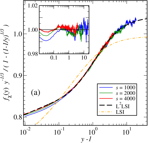
Figure 3: (a) Scaling of the integrated autoresponse $\chi(t,s)=s^{+1/3}f_{\chi}(t/s)$ of the $1D$ Kardar-Parisi-Zhang equation, as a function of $y=t/s$, for several values of the waiting time $s$. The figure shows the reduced scaling function $f_{\rm red}(y)=f_{\chi}(y)y^{-1/3}\left[1-(1-y^{-1})^{1/3}\right]^{-1}$. The dash-dotted line labelled lsi gives a fit to non-logarithmic lsi (see text) and the dashed line labelled l²lsi gives the prediction (6.5). The inset shows the ratio $f_{\chi}(y)/f_{\rm L^{2}LSI}(y)$ over against $y$.
(b) Reduced scaling function $h_{R}(y)=f_{R}(y)y^{\lambda_{R}/z}(1-1/y)^{1+a}$ the autoresponse $R(t,s)=s^{-1-a}f_{R}(t/s)$ of the $1D$ critical contact process, as a function of $y=t/s$, for several values of the waiting time $s$. The dashed line labelled ‘lsi’ is from (5.9), with $a^{\prime}-a=0.26$. The full curve labelled ‘l²lsi’ is obtained from eq. (6.7), derived from logarithmic lsi with $f_{0}=0$, see text. After [48, 51].

In figure 3a, the simulational data from [48] are compared with the predicted form (6.5). Very large values of the waiting time $s$ are required, and one may observe from figure 3a that even data with $s<10^{3}$ are not yet fully in the scaling regime. While non-logarithmic lsi gives an overall agreement with an accuracy up to about $5\%$, when $a^{\prime}=-0.5$ is assumed, clear and systematic deviations remain. It turns out that if one tried to use the more restricted prediction (2.29) of logarithmic Schrödinger-invariance (without the second scaling dimension), the numerical result is indistinguishable from non-logarithmic lsi [51]. However, the prediction (6.5) reproduces the data to an accuracy better than $0.1\%$ and at least down to $y=t/s\approx 1.03$ (the inset shows that this is about the region where the numerical data obey dynamical scaling), with the fitted values $a^{\prime}=-0.8206$, $A_{0}=0.7187$, $A_{1}=0.2424$ and $A_{2}=-0.09087$.

6.2 One-dimensional critical directed percolation

The directed percolation universality class is usually considered to most simple example of a non-equilibrium phase transition with an absorbing state. It has been realised in countless different ways, with often-used examples being either the contact process or else Reggeon field theory, and very precise estimates of the location of the critical point and the critical exponents are known, see [52, 85, 45] and references therein. Its predictions are also in agreement with extensive recent experiments in turbulent liquid crystals [99]. Since it is well-understood that critical $2D$ isotropic percolation can be described in terms of conformal invariance [70], one might wonder whether some kind of local scale-invariance might be applied to directed percolation.

In the contact process, a response function can be defined by considering the response of the time-dependent particle concentration with respect to a time-dependent particle-production rate. In figure 3b, numerical data for the rescaled scaling function

$$h_{R}(y):=f_{R}(y)y^{\lambda_{R}/z}(1-y^{-1})^{1+a}$$ (6.6)

are shown, where the values of the exponents are taken from [45]. An excellent data collapse is seen. Non-logarithmic lsi, and assuming $a^{\prime}-a=0.26$, describes the data well down to about $y\approx 1.1$, but systematic deviations remain.

In order to compare the data with logarithmic lsi, we make the same working assumptions as before for KPZ. With $x^{\prime}=\widetilde{x}^{\prime}=0$, logarithmic lsi eq. (5.7) predicts

$$h_{R}(y) = \left(1-\frac{1}{y}\right)^{a-a^{\prime}}\left(h_{0}-g_{12,0}\widetilde{\xi}^{\prime}\ln(1-1/y)-\frac{1}{2}f_{0}\widetilde{\xi}^{\prime 2}\ln^{2}(1-1/y)\right.$$ (6.7)

$$\left.~{}~{}~{}~{}~{}~{}-g_{21,0}\xi^{\prime}\ln(y-1)+\frac{1}{2}f_{0}\xi^{\prime 2}\ln^{2}(y-1)\right)$$

Further constraints must be obeyed, in particular the resulting scaling function should always be positive.

Numerical experiments reveal that the best fits are obtained by fitting the generic form (6.7) to the data. It then turns out that the terms which depend quadratically on the logarithms have amplitudes which are about $10^{-4}$ times smaller than those of the other terms. We consider this as evidence that $f_{0}=0$. This gives the phenomenological scaling form $h_{R}(y)=h_{0}(1-1/y)^{a-a^{\prime}}\left(1-(A+B)\ln(1-1/y)+B\ln(y-1)\right)$, where $h_{0}$ is a normalisation constant and $A,B$ are two positive universal parameters. With the fitted parameters $a-a^{\prime}=0.00198$, $A=0.407$, $B=0.02$ and $h_{0}=0.08379$, this gives a good description of the data, down to $y-1\approx 2\cdot 10^{-3}$. (for smaller values of $y$, we cannot be sure to be still in the scaling regime).

Note that the estimate $a^{\prime}-a\simeq-0.002$ is quite distinct from the earlier estimate $a^{\prime}=a\approx 0.27$ [43] and also implies a small logarithmic contribution in the $y\gg 1$ limit.

Similar results have also been obtained for the critical $2D$ voter model on a triangular lattice. This will be reported elsewhere [50].

7 Conclusions

We have presented current ideas on the analogues of logarithmic conformal invariance in non-relativistic contexts. Several formal developments can be carried out in quite close analogy with the well-known conformal case, but the possibility of true projective representations and the absence of time-translation-invariance in several physical applications leads to new features, absent from conformal invariance.

Up to date, the only physical applications studied involve slow relaxation phenomena far from equilibrium. It appears that non-equilibrium scaling operators are to be described in terms of two, rather than one, independent scaling exponents, which we labeled here $x$ and $\xi$; and furthermore, in the known physical examples it seem that only the elusive second scaling dimension $\xi$ is extended to a Jordan matrix and thus carries the essential logarithmic structure. Further work will without doubt inform us in the future to what extent this appreciation will remain valid.

In any case, in very commonly studied models of non-equilibrium statistical physics, NRLCFTs have found their first applications.

Acknowledgement: We thank the organisers of the meeting “Advanced conformal field theory” at the Institut Poincaré in Paris for their warm hospitality. MH was partly supported by the Collège Doctoral franco-allemand Nancy-Leipzig-Coventry (Systèmes complexes à l’èquilibre et hors èquilibre) of UFA-DFH.

References

- [1] M. Alishahiha, A. Davody and A. Vahedi, JHEP 0908, 022 (2009) [arXiv:0903.3953].
- [2] A. Bagchi and I. Mandal, Phys. Lett. B675, 393 (2009). [arxiv:0903.0580]
- [3] A. Bagchi, R. Gopakumar, I. Mandal and A. Miwa, [arxiv:0912.1090].
- [4] K. Balasubramanian and J. McGreevy, Phys. Rev. Lett. 101, 061601 (2008). [arxiv:0804.4053]
- [5] A.L. Barabási and H.E. Stanley, Fractal concepts in surface growth, Cambridge University Press (1995).
- [6] V. Bargman, Ann. of Math. 56, 1 (1954).
- [7] A.O. Barut, Helv. Phys. Acta, 46, 496-503 (1973).
- [8] M.T. Batchelor, R.V. Burne, B.I. Henry and S.D. Watt, Physica A282, 123 (2000).
- [9] A.A. Belavin, A.M. Polyakov and A.B. Zamolodchikov, Nucl. Phys. B241, 333 (1984).
- [10] A.J. Bray, Adv. Phys. 43, 357 (1994).
- [11] G. Burdet, M. Perrin and P. Sorba, Comm. Math. Phys. 34, 85-90 (1973).
- [12] S. Bustingorry, J. Stat. Mech. P10002 (2007) [arxiv:0708.2615];
- [13] P. Calabrese and P. Le Doussal, Phys. Rev. Lett. 106, 250603 (2011) [arxiv:1104.1993]; J. Stat. Mech. P06001 (2012) [arxiv:1204.2607]
- [14] J.L. Cardy, J. Phys. A25, L201 (1992).
- [15] J.L. Cardy, Scaling and renormalisation in statistical physics, Cambridge University Press (1996).
- [16] J.-S. Caux, I.I. Kogan and A.M. Tsvelik, Nucl. Phys. B466, 444 (1996). [hep-th/9511134]
- [17] R. Cherniha and M. Henkel, J. Math. Anal. Appl. 369, 120 (2010). arxiv:0910.4822]
- [18] Y.-L. Chou and M. Pleimling, J. Stat. Mech. 2010, P08007 (2010) [arxiv:1007.2380].
- [19] I. Corwin, Rand. Matrices: Theory and Appl. 1, 1130001 (2012) [arxiv:1106.1596v4]
- [20] L.F. Cugliandolo, in Slow Relaxation and non equilibrium dynamics in condensed matter, Les Houches Session 77 July 2002, J-L Barrat, J Dalibard, J Kurchan, M V Feigel’man eds, Springer(Heidelberg 2003) (cond-mat/0210312).
- [21] G. L. Daquila and U. C. Täuber, Phys. Rev. E83, 051107 (2011) [arxiv:1102.2824]; and Phys. Rev. Lett. 108, 110602 (2012) [arxiv:1112.1605].
- [22] I. Dornic, H. Chaté, J. Chave and H. Hinrichsen, Phys. Rev. Lett. 87, 045701 (2001) [cond-mat/0101202].
- [23] C. Duval and P.A. Horváthy, J. Phys. A: Math. Theor. 42, 465206 (2009). [arxiv:0904.0531]
- [24] T. Enss, M. Henkel, A. Picone and U. Schollwöck, J. Phys. A37, 10479 (2004). [cond-mat/0410147]
- [25] C.A. Fuertes and S. Moroz, Phys. Rev. D79, 106004 (2009). [arxiv:0903.1844]
- [26] M.R. Gaberdiel and H.G. Kausch, Phys. Lett. B386, 131 (1996) [hep-th/9606050]; Nucl. Phys. B538, 631 (1999) [hep-th/9807091].
- [27] T. Geudre and P. Le Doussal, [arxiv:1208.5669].
- [28] D. Giulini, Ann. of Phys. 249, 222 (1996).
- [29] C. Godrèche and J.M. Luck, J. Phys. A. Math. Gen. 33, 1151 (2000). [cond-mat/9911348]
- [30] N. Gray, D. Minic and M. Pleimling, [arxiv:1301.6368].
- [31] S. S. Gubser, I. R. Klebanov and A. M. Polyakov, Phys. Lett. B428, 105 (1998). [hep-th/9802109]
- [32] V. Gurarie, Nucl. Phys. B410, 535 (1993). [hep-th/9303160]
- [33] V. Gurarie, M. Flohr and C. Nayak, Nucl. Phys. B498, 513 (1997). [cond-mat/9701212]
- [34] C. R. Hagen, Phys. Rev. D5, 377 (1972).
- [35] T. Halpin-Healy and Y.-C. Zhang, Phys. Rep. 254, 215 (1995).
- [36] S.A. Hartnoll, Class. Quant. Grav. 26, 224002 (2009). [arxiv:0903.3246]
- [37] M. Hassaïne and P.A. Horváthy, Ann. of Phys. 282, 218 (2000) [math-ph/9904022]; Phys. Lett. A279, 215 (2001) [hep-th/0009092].
- [38] P. Havas and J. Plebanski, J. Math. Phys. 19, 482 (1978).
- [39] M. Henkel, J. Stat. Phys. 75, 1023 (1994). [hep-th/9310081]
- [40] M. Henkel, Phys. Rev. Lett. 78, 1940 (1997). [cond-mat/9610174]
- [41] M. Henkel, Nucl. Phys. B641, 405 (2002). [hep-th/0205256]
- [42] M. Henkel and J. Unterberger, Nucl. Phys. B660, 407 (2003). [hep-th/0302187]
- [43] M. Henkel, T. Enss and M. Pleimling, J. Phys. A Math. Gen. 39, L589 (2006) [cond-mat/0605211].
- [44] M. Henkel, R. Schott, S. Stoimenov and J. Unterberger, Confluentes Mathematici 4, 1250006 (2012) [math-ph/0601028].
- [45] M. Henkel, H. Hinrichsen and S. Lübeck, Non-equilibrium phase transitions vol. 1: absorbing phase transitions, Springer (Heidelberg 2009).
- [46] M. Henkel and M. Pleimling, Non-equilibrium phase transitions vol. 2: ageing and dynamical scaling far from equilibrium, Springer (Heidelberg 2010).
- [47] M. Henkel and S. Stoimenov, Nucl. Phys. B847, 612 (2011). [arxiv:1011.6315]
- [48] M. Henkel, J.D. Noh and M. Pleimling, Phys. Rev. E85, 030102(R) (2012). [arxiv:1109.5022]
- [49] M. Henkel, in proceedings of 7th workshop on Algebra, Geometry, Mathematical Physics (AGMP-7), Mulhouse 24-26 oct 2011, [arxiv:1205.5901].
- [50] M. Henkel and F. Sastre, work in progress.
- [51] M. Henkel, Nucl. Phys. B869, 282 (2013). [arxiv:1009.4139]
- [52] H. Hinrichsen, Adv. Phys. 49, 815 (2000). [cond-mat/0001070]
- [53] P.A. Horváthy, L. Martina and P.C. Stichel, SIGMA 6, 060 (2010).
- [54] A. Hosseiny and S. Rouhani, J. Math. Phys. 51 102303 (2010) [arxiv:1001.1036].
- [55] Hosseiny, A., M. Henkel, and S. Rouhani. “The logarithmic exotic Galilean conformal algebra,” work in progress.
- [56] S. Hyun, J. Jeong and B.S. Kim, Aging logarithmic conformal field theory : a holographic view, [arxiv:1209.2417].
- [57] E.V. Ivashkevich, J. Phys. A: Math. Gen. 30, L525 (1997). [hep-th/9610221]
- [58] R. Jackiw, Physics Today 25, 23 (1972).
- [59] C.G. Jacobi, Vorlesungen über Dynamik (1842/43), 4. Vorlesung, in “Gesammelte Werke”, A. Clebsch und E. Lottner (eds), Akademie der Wissenschaften (Berlin 1866/1884)
- [60] H.K. Janssen, in G. Gyórgi et al. (eds), From phase transitions to chaos, World Scientific (Singapour 1992).
- [61] J.I. Jottar, R.G. Leigh, D. Minic and L.A. Pando Zayas, JHEP 1011:034 (2010) [arxiv:1004.3752].
- [62] H. Kallabis and J. Krug, Europhys. Lett. 45, 20 (1999). [cond-mat/9809241]
- [63] M. Kardar, G. Parisi and Y.-C. Zhang, Phys. Rev. Lett. 56, 889 (1986).
- [64] H.A. Kastrup, Nucl. Phys. B7, 545 (1968).
- [65] J.M. Kim and J.M. Kosterlitz, Phys. Rev. Lett. 62, 2289 (1989).
- [66] A.W. Knapp, “Representation theory of semisimple groups: an overview based on examples”, Princeton Univ. Press (Princeton 1986).
- [67] M. Krech, Phys. Rev. E55, 668 (1997). [cond-mat/9609230]
- [68] T. Kriecherbauer and J. Krug, J. Phys. A43, 403001 (2010). [arxiv:0803.2796]
- [69] J. Krug, Adv. Phys. 46, 139 (1997).
- [70] R. Langlands, P. Pouloit and Y. Saint-Aubin, Bull. Am. Math. Soc. 30, 1 (1994).
- [71] R.G. Leigh and N.N. Hoang, JHEP 0911:010 (2009) [arxiv:0904.4270].
- [72] R.G. Leigh and N.N. Hoang, JHEP 1003:027 (2010) [arxiv:0909.1883].
- [73] S. Lie, Über die Integration durch bestimmte Integrale von einer Klasse linearer partieller Differentialgleichungen, Arch. for Mathematik og Naturvidenskab, 6, 328 (1881).
- [74] J. Lukierski, P.C. Stichel and W.J. Zakrewski, Phys. Lett. A357, 1 (2006) [hep-th/0511259]; Phys. Lett. B650, 203 (2007) [hep-th/0702179].
- [75] J.M. Maldacena, Adv. Theor. Math. Phys. 2, 231 (1998). [hep-th/9711200]
- [76] D. Martelli and Y. Tachikawa, JHEP 1005:091 (2010). [arxiv:0903.5184]
- [77] P. Mathieu and D. Ridout, Phys. Lett. B657, 120 (2007) [arxiv:0708.0802]; and Nucl. Phys. B801, 268 (2008) [arxiv:0711.3541].
- [78] S. Mathieu and P. Ruelle, Phys. Rev. E64, 066130 (2001). [hep-th/0107150]
- [79] D. Minic, D. Vaman and C. Wu, Phys. Rev. Lett. 109, 131601 (2012). [arxiv:1207.0243].
- [80] S. Moghimi-Araghi, S. Rouhani and M. Saadat, Nucl. Phys. B599, 531 (2000) [hep-th/0008165].
- [81] Yu. Nakayama, J. High-energy Phys. 04, 102 (2010). [arxiv:1002.0615]
- [82] J. Negro, M.A. del Olmo and A. Rodríguez-Marco, J. Math. Phys. 38, 3786 (1997).
- [83] U. Niederer, Helv. Phys. Acta 45, 802 (1972).
- [84] U. Niederer, Helv. Phys. Acta 51, 220 (1978).
- [85] G. Ódor, Rev. Mod. Phys. 76, 663 (2004). [cond-mat/0205644]
- [86] L. O’Raifeartaigh and V.V. Sreedhar, Ann. of Phys. 293, 215 (2001).
- [87] L.V. Ovsiannikov, The Group Analysis of Differential Equations, Academic Press (London 1980).
- [88] V. Ovsienko and C. Roger, Indag. Math. 9, 277 (1998).
- [89] A. Picone and M. Henkel, Nucl. Phys. B688 217 (2004). [cond-mat/0402196]
- [90] A.M. Polyakov, Sov. Phys. JETP Lett. 12, 381 (1970).
- [91] M.R. Rahimi Tabar and S. Rouhani, EPL 37, 447 (1997)
- [92] J.J. Ramasco, M. Henkel, M.A. Santos, C. da Silva Santos, J. Phys. A37, 10497 (2004). [cond-mat/0406146]
- [93] C. Roger and J. Unterberger, Ann. Inst. H. Poincaré 7, 1477 (2006).
- [94] H. Saleur, Nucl. Phys. B382, 486 (1992). [hep-th/9111007]
- [95] T. Sasamoto and H. Spohn, J. Stat. Mech. P11013 (2010). [arxiv:1010.2691]
- [96] T. Sasamoto and H. Spohn, Phys. Rev. Lett. 104, 230602 (2010). [arxiv:1002.1883]
- [97] D.T. Son, Phys. Rev. D78, 106005 (2008). [arxiv:0804.3972]
- [98] S. Stoimenov and M. Henkel, [arxiv:1212.6156]
- [99] K.A. Takeuchi, M. Kuroda, H. Chaté and M. Sano, Phys. Rev. Lett. 99, 234503 (2009) [arxiv:0706.4151] – err. 103, 089901(E) (2009); and Phys. Rev. E80, 051116 (2009) [arxiv:0907.4297].
- [100] K.A. Takeuchi, M. Sano, T. Sasamoto and H. Spohn, Scientific Reports 1:34 (2011) [arxiv:1108.2118]; K.A. Takeuchi and M. Sano, Phys. Rev. Lett. 104, 230601 (2010) [arxiv:1001.5121] and J. Stat. Phys. 147, 853 (2012) [arxiv:1203.2530].
- [101] W.M. Tong and R.S. Williams, Ann. Rev. Phys. Chem. 45, 401 (1994).
- [102] J. Unterberger and C. Roger, The Schrödinger-Virasoro algebra, Springer (Heidelberg 2012).
- [103] G.M.T. Watts, J. Phys. A29, L363 (1996). [cond-mat/9603167]
- [104] E. Witten, Adv. Theor. Math. Phys. 2, 253 (1998) [hep-th/9802150].
- [105] P.-M. Zhang and P.A. Horváthy, Eur. Phys. J. C65, 607 (2010). [arxiv:0906.3594]