Spontaneous fission half-lives of heavy and superheavy nuclei within a generalized liquid drop model

Abstract

We systematically calculate the spontaneous fission half-lives for heavy and superheavy nuclei between U and Fl isotopes. The spontaneous fission process is studied within the semi-empirical WKB approximation. The potential barrier is obtained using a generalized liquid drop model, taking into account the nuclear proximity, the mass asymmetry, the phenomenological pairing correction, and the microscopic shell correction. Macroscopic inertial-mass function has been employed for the calculation of the fission half-life. The results reproduce rather well the experimental data. Relatively long half-lives are predicted for many unknown nuclei, sufficient to detect them if synthesized in a laboratory.

1. School of Nuclear Science and Technology, Lanzhou University, Lanzhou 730000, China

2. Laboratoire Subatech, UMR: IN2P3/CNRS-Université-Ecole des Mines, 4 rue A. Kastler, 44 Nantes, France

3. Institute of Modern Physics, Chinese Academy of Science, Lanzhou 730000, China

Keywords: heavy and superheavy nuclei; half-lives; spontaneous fission

1 Introduction

Spontaneous fission of heavy nuclei was first predicted by Bohr and Wheeler in 1939 [1]. Their fission theory was based on the liquid drop model. Interestingly, their work also contained an estimate of a lifetime for fission from the ground state. Soon afterwards, Flerov and Petrzak [2] presented the first experimental evidence for spontaneous fission. Since this discovery of spontaneous fission of ²³⁸U, fission of numerous other actinide nuclei have been reported experimentally [3]. Several theoretical approaches, both phenomenologically and microscopically, can be employed to investigate spontaneous fission. Early descriptions of fission were based on a purely geometrical framework of the charged liquid drop model [1]. In 1955 Swiatecki [4] suggested that more realistic fission barriers could be obtained by adding a correction energy to the minimum in the liquid drop model barrier. The correction was calculated as the difference between the experimentally observed nuclear ground-state mass and the mass given by the liquid drop model. Swiatecki obtained much improved theoretical spontaneous fission half-lives based on these modified liquid drop model barriers. These observations formed the basis for the shell-correction method. In the mid-1960s, Strutinsky [5, 6] presented a method to theoretically calculate these shell corrections. Quantum shell effects are added to the average behavior described by the liquid drop. This macroscopic-microscopic approach turned out to be very successful in explaining many features of spontaneous fission [7, 8, 9]. As compared to $\alpha$-decay, the spontaneous fission is much more complex and there are some data such as mass and charge numbers of the two fragments, number of emitted neutrons and released energy, …which are very difficult to reproduce. The full microscopic treatment of such a multidimensional system is extremely complex. In particular, a microscopic calculation of spontaneous fission half-lives is very difficult due to both the complexity of the fission process and the uncertainty on the height and shape of the fission barrier [10, 11]. Indeed, the deformation energy of the nucleus undergoes a significant change when the nuclear shape turns into a strongly deformed configuration of two fragments in contact at the scission point. Furthermore, it is known that the spontaneous fission half-life is very sensitive to small changes of the various quantities appearing in the calculations.

Spontaneous fission is one of the most prominent decay modes, energetically feasible for heavy and superheavy nuclei(SHN). Recently, the spontaneous fission half-lives of several SHN have been measured by different laboratories [12, 13, 14, 15, 16, 17]. The fission as well as $\alpha$-decay probability determines the stability of these newly synthesized SHN.

Within a Generalized Liquid Drop Model (GLDM) taking into account the mass and charge asymmetry and the proximity energy, the deformation energy of compact and creviced shapes have been determined. The proximity forces strongly lower the deformation energy of these quasimolecular shapes and the calculated fission barrier heights agree well with the experimental results [18, 19, 20, 21]. Within the same approach, the $\alpha$-decay [22, 23, 24, 25], cluster emission [26] and fusion [27] data can also be reproduced.

The present work is closely connected with the intensive experimental activity on the synthesis and study of heavy and SHN in recent years. It aims at the interpretation of existing experimental fission half-lives and in predictions of half-lives of yet unknown nuclei. By using the GLDM and taking into account the ellipsoidal deformations of the two different fission fragments and their associated microscopic shell corrections and pairing effects, we have systematically calculated the spontaneous fission half-lives of nuclei in the mass region from ²³²U to ²⁸⁶Fl by considering all the possible mass and charge asymmetries.

The study is focused on quasimolecular shapes since these shapes have been rarely investigated in the past. Indeed, this quasimolecular shape valley where the nuclear proximity effects are so important is inaccessible in using the usual development of the nuclear radius. Furthermore, microscopic studies within HFB theory cannot describe the evolution of two separated fragments and cannot simulate the formation of a deep neck between two almost spherical fragments. The reproduction of the proximity energy is also not obvious within mean-field approaches and the definition of the scission point is not easy for very elongated shapes.

The paper is organized as follows. The selected shape sequence and macroscopic-microscopic model are described in Section 2, results and discussions are given in Section 3, and conclusions and summary are presented in Section 4.

2 Shape sequence and macroscopic-microscopic model

2.1 Quasimolecular shapes

The shape is given simply in polar coordinates (in the plane $\phi=0$) by [28]

$$R(\theta)^{2}=\begin{cases}a^{2}\sin^{2}\theta+c_{1}\cos^{2}\theta~{}~{}(0\leq\theta\leq\pi/2)\\ a^{2}\sin^{2}\theta+c_{2}\cos^{2}\theta~{}~{}(\pi/2\leq\theta\leq\pi)\end{cases}$$ (2.1)

where $c_{1}$ and $c_{2}$ are the two radial elongations and $a$ is the neck radius. Assuming volume conservation, the two parameters $s_{1}=a/c_{1}$ and $s_{2}=a/c_{2}$ completely define the shape. The radii of the future fragments allow to connect $s_{1}$ and $s_{2}$:

$$s_{2}^{2}=\frac{s_{1}^{2}}{s_{1}^{2}+(1-s_{1}^{2})(R_{2}/R_{1})^{2}}.$$ (2.2)

When $s_{1}$ decreases from 1 to 0 the shape evolves continuously from one sphere to two touching spheres with the natural formation of a deep neck while keeping almost spherical ends. So, we would like to point out that the most attractive feature of the quasimolecular shapes is that it can describe the process of the shape evolution from one body to two separated fragments in a unified way.

2.2 GLDM energy

Within GLDM the macroscopic energy of a deformed nucleus is defined as

$$E=E_{V}+E_{S}+E_{C}+E_{prox},$$ (2.3)

where the different terms are respectively the volume, surface, Coulomb and nuclear proximity energies.
For one-body shapes, the volume $E_{V}$, surface $E_{S}$ and Coulomb $E_{C}$ energies are given by

$$E_{V}=-15.494(1-1.8I^{2})A~{}MeV,$$ (2.4)

$$E_{S}=17.9439(1-2.6I^{2})A^{2/3}(S/4\pi R_{0}^{2})~{}MeV,$$ (2.5)

$$E_{C}=0.6e^{2}(Z^{2}/R_{0})B_{C}.$$ (2.6)

$B_{C}$ is the Coulomb shape dependent function, $S$ is the surface and $I$ is the relative neutron excess.

$$B_{C}=0.5\int(V(\theta)/V_{0})(R(\theta)/R_{0})^{3}\sin\theta d\theta,$$ (2.7)

where $V(\theta)$ is the electrostatic potential at the surface and $V_{0}$ is the surface potential of the sphere. The effective sharp radius $R_{0}$ has been chosen as

$$R_{0}=(1.28A^{1/3}-0.76+0.8A^{-1/3})~{}fm.$$ (2.8)

This formula proposed in Ref. [29] is derived from the droplet model and the proximity energy and simulates rather a central radius for which $R_{0}/A^{1/3}$ increases slightly with the mass. It has been shown [22, 27] that this selected more elaborated expression can also be used to reproduce accurately the fusion, fission, cluster and alpha decay data.

For two-body shapes, the coaxial ellipsoidal deformations have been considered [30]. The system configuration depends on two parameters: the ratios s_i ($i=1,2$) between the transverse semi-axis $a_{i}$ and the radial semi-axis $c_{i}$ of the two different fragments

$$a_{i}=R_{i}s_{i}^{1/3}~{}~{}and~{}~{}c_{i}=R_{i}s_{i}^{-2/3}.$$ (2.9)

The prolate deformation is characterized by s$\leq$1 and the related eccentricity is written as $e^{2}=1-s^{2}$ while in the oblate case s$\geq$1 and $e^{2}=1-s^{-2}$. The volume and surface energies are $E_{V_{12}}=E_{V_{1}}+E_{V_{2}}$ and $E_{S_{12}}=E_{S_{1}}+E_{S_{2}}$. In the prolate case, the relative surface energy reads

$$B_{Si}=\frac{(1-e_{i}^{2})^{1/3}}{2}[1+\frac{\sin^{-1}(e_{i})}{e_{i}(1-e_{i}^{2})^{1/2}}]$$ (2.10)

and in the oblate case

$$B_{Si}=\frac{(1+\epsilon_{i}^{2})^{1/3}}{2}[1+\frac{\ln(\epsilon_{i}+(1+\epsilon_{i}^{2})^{1/2})}{\epsilon_{i}(1+\epsilon_{i}^{2})^{1/2}}],$$ (2.11)

where $\epsilon_{i}^{2}=s_{i}^{2}-1$.

The Coulomb self-energy of the spheroid $i$ is

$$E_{C,self}=\frac{3e^{2}Z_{i}^{2}B_{ci}}{5R_{i}}.$$ (2.12)

The relative self-energy is, in the prolate case

$$B_{Ci}=\frac{(1-e_{i}^{2})^{1/3}}{2e_{i}}\ln\frac{1+e_{i}}{1-e_{i}}$$ (2.13)

and in the oblate case

$$B_{Ci}=\frac{(1+\epsilon_{i}^{2})^{1/3}}{\epsilon_{i}}\tan^{-1}\epsilon_{i}.$$ (2.14)

The Coulomb interaction energy between the two fragments reads

$$E_{C,int}=\frac{e^{2}Z_{1}Z_{2}}{r}[s(\lambda_{1})+s(\lambda_{2})-1+S(\lambda_{1},\lambda_{2})]$$ (2.15)

where $\lambda_{i}^{2}=(c_{i}^{2}-a_{i}^{2})/r^{2}$, $r$ is the distance between the two mass centers.

In the prolate case, s$(\lambda_{i})$ is expressed as

$$s(\lambda_{i})=\frac{3}{4}(\frac{1}{\lambda_{i}}-\frac{1}{\lambda_{i}^{3}})\ln(\frac{1+\lambda_{i}}{1-\lambda_{i}})+\frac{3}{2\lambda_{i}^{2}},$$ (2.16)

while for the oblate shapes

$$s(\lambda_{i})=\frac{3}{2}(\frac{1}{\omega_{i}}+\frac{1}{\omega_{i}^{3}})\tan^{-1}\omega_{i}-\frac{3}{2\omega_{i}^{2}},$$ (2.17)

where $\omega_{i}^{2}=-\lambda_{i}^{2}$.

$S(\lambda_{1},\lambda_{2})$ can be represented in the form of a two-fold summation

$$S(\lambda_{1},\lambda_{2})=\sum_{j=1}^{\infty}\sum_{k=1}^{\infty}\frac{3}{(2j+1)(2j+3)}$$ (2.18)

$$\frac{3}{(2k+1)(2k+3)}\frac{(2j+2k)!}{(2j)!(2k)!}\lambda_{1}^{2j}\lambda_{2}^{2k}.$$

The surface energy results from the effects of the surface tension forces in a half space. When a neck or a gap appears between separated fragments an additional term called proximity energy must be added to take into account the effects of the nuclear forces between the close surfaces. It moves the barrier top to an external position and strongly decreases the pure Coulomb barrier:

$$E_{prox}(r)=2\gamma\int_{h_{min}}^{h_{max}}\Phi[D(r,h)/b]2\pi hdh$$ (2.19)

where

$$\gamma=0.9517\sqrt{(1-2.6I_{1}^{2})(1-2.6I_{2}^{2})}MeVfm^{-2}.$$ (2.20)

$h$ is the transverse distance varying from the neck radius or zero to the height of the neck border, $D$ is the distance between the opposite surfaces in consideration and $b$ is the surface width fixed at 0.99 fm. $\Phi$ is the proximity function. The surface parameter $\gamma$ is the geometric mean between the surface parameters of the two fragments.

2.3 Shell energy

The shape-dependent shell corrections have been determined within the Droplet Model expressions [31]:

$$E_{shell}=E_{shell}^{sphere}(1-2.0\alpha^{2})e^{-\alpha^{2}}$$ (2.21)

where $\alpha^{2}=(\delta R)^{2}/a^{2}$. The distortion $\alpha$a is the root mean square of the deviation of the surface from a sphere, a quantity which incorporates all types of deformation indiscriminately. The range a has been chosen to be 0.32r₀. The whole shell correction energy decreases to zero with increasing distortion of the nucleus due to the attenuating factor ($e^{-\alpha^{2}}$). The Strutinsky method at large deformations supposes that the nucleon shells are not affected by the proximity effects, which is highly improbable when there are a deep neck in the deformed shape and close surfaces in regard.

The $E_{shell}^{sphere}$ is the shell corrections for a spherical nucleus,

$$E_{shell}^{sphere}=cE_{sh}$$ (2.22)

and is obtained by the Strutinsky method by setting the smoothing parameter $\gamma=1.15~{}~{}\hbar\omega_{0}$ and the order $p=6$ of the Gauss-Hermite polynomials, where $\hbar\omega_{0}=41A^{-1/3}$ MeV is the mean distance between the gross shells, the sum of the shell energies of protons and neutrons. Meanwhile, we introduce a scale factor c to the shell correction. In this work, we choose $c=0.82$. To obtain the shell correction $E_{shell}^{sphere}$, we calculate the single-particle levels based on an axially deformed Woods-Saxon potential and then apply the Strutinsky method. The single-particle Hamiltonian is written as [32],

$$H=T+V+V_{S.O},$$ (2.23)

with the spin-orbit potential

$$V_{S.O}=-\lambda(\frac{\hbar}{2Mc})^{2}\nabla V\cdot(\vec{\sigma}\times\vec{p}),$$ (2.24)

where $M$ is the free nucleonic mass, $\vec{\sigma}$ is the Pauli spin matrix and $\vec{p}$ is the nucleon momentum. $\lambda$ means the strength of the spin-orbit potential. Here we set $\lambda=\lambda_{0}(1+N_{i}/A)$ with $N_{i}=Z$ for protons and $N_{i}=N$ for neutrons and $\lambda_{0}$ value of 26.3163. The central potential $V$ is described by an axially deformed Woods-Saxon form

$$V(\vec{r})=\frac{V_{q}}{1+\exp[\frac{r-R(\theta)}{a}]},$$ (2.25)

where the depth $V_{q}$ of the central potential ($q=p$ for protons and $q=n$ for neutrons) is written as

$$V_{q}=V_{0}\mp V_{S}I,$$ (2.26)

with the minus sign for protons and the plus sign for neutrons. $V_{0}$ and a take the values -47.4784 and 0.7842, respectively. $V_{S}$ and $I$ are the isospin-asymmetric part of the potential depth and the relative neutron excess, where

$$V_{S}=c_{sym}[1-\frac{\kappa}{A^{1/3}}+\frac{2-|I|}{2+|I|A}].$$ (2.27)

The values of $c_{sym}$ and $\kappa$ are 29.2876 and 1.4492, respectively [33].

2.4 Pairing energy

The shape-dependent pairing energy has been calculated with the following expressions of the finite-range droplet model [34].

For odd Z, odd N numbers :

$$E_{Pairing}=\frac{4.8B_{S}}{N^{1/3}}+\frac{4.8B_{S}}{Z^{1/3}}-\frac{6.6}{B_{S}A^{2/3}}.$$ (2.28)

For odd Z, even N numbers :

$$E_{Pairing}=\frac{4.8B_{S}}{Z^{1/3}}.$$ (2.29)

For even Z, odd N numbers :

$$E_{Pairing}=\frac{4.8B_{S}}{N^{1/3}}.$$ (2.30)

For even Z, even N numbers :

$$E_{Pairing}=0.$$ (2.31)

The relative surface energy $B_{s}$, which is the ratio of the surface area of the nucleus at the actual shape to the surface area of the nucleus at the spherical shape, is given by

$$B_{s}=\frac{\int_{S}dS}{S_{sphere}}.$$ (2.32)

The pairing energies vary with $B_{s}$.

Within this asymmetric fission model the decay constant is simply given by $\lambda_{i}=\nu_{0}$P_i, and the assault frequency $\nu_{0}$ has been taken as $\nu_{0}=10^{20}$s^-1. The barrier penetrability P_i is calculated within the action integral

$$P_{i}=\exp[-\frac{2}{\hbar}\int_{r_{1}}^{r_{2}}\sqrt{2B(r)(E(r)-E(sphere))}dr].$$ (2.33)

The limits of integration $r_{1}$ and $r_{2}$ are the points of entrance and exit, respectively, into and from the barrier. The function $B(r)$ is the inertia with respect to $r$ associated with motion in the fission direction. The fission half-lives have been calculated within the following semi-empirical model for the inertia [35]

$$B(r)=\mu(1+k\exp[-\frac{128}{51}(r-R_{sph}/R_{0})])$$ (2.34)

where $\mu$ is the reduced mass of the final fragments and $k$ is a semi-empirical constant, $k=14.8$. $R_{sph}$ is the distance between the mass centers of the future fragments in the initial sphere, $R_{sph}/R_{0}=0.75$ in the symmetric case. To obtain the total fission constant $\lambda$, we have calculated all the possible spontaneous fission half-lives corresponding to fission constant $\lambda_{i}$ of the different possible exiting channels depending on the different mass and charge asymmetries. The calculated half-lives of all possible ²³⁴U spontaneous fission channels are shown in Fig.1 versus one of daughter nucleus mass number for illustration of the method. For given Z₁ and Z₂ values the spontaneous fission half-lives decrease with one fragment mass number A₂, reach a minimum and then increase with increasing A₂. The total fission constant is $\lambda$=$\lambda_{1}+\lambda_{2}....+\lambda_{n}$ and the half-life is finally obtained by $T_{1/2}=(\ln 2)/\lambda$.

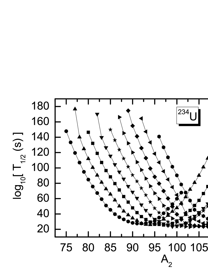
Figure 1: Calculated spontaneous fission half-lives for ²³⁴U as a function of one of daughter nucleus mass number. Parabolic half-live curves represent the different Z₁ and Z₂ combinations, where Z₁ and Z₂ indicate the proton numbers of the two fragments for ²³⁴U spontaneous fission.

3 Results and discussions

The spontaneous fission half-lives of nuclei from ²³²U to ²⁸⁶Fl have been systematically calculated by using the GLDM taking into account the microscopic shell corrections and the shape-dependent pairing energy. The results are listed in Table 1. The first and fourth columns indicate the spontaneous fissioning nuclei. The experimental [17, 36] and theoretical spontaneous fission half-lives are compared in the other columns. The spontaneous fission half-lives vary in an extremely wide range from $10^{26}$ seconds to $10^{-3}$ seconds when the nucleon number varies from A=232 to A=286. For a variation nucleon number less than 60, the amplitude of variation of spontaneous fission half-lives is as high as $10^{29}$. This leads to the extreme sensitivity of the half-lives to nucleon number. Thus it is a very difficult task to reproduce the experimental data accurately. However, the theoretical spontaneous fission half-lives are in good agreement with the experimental ones. Among 47 nuclei, 37 experimental half-lives can be reproduced within a factor of $10^{2}$. Only for 7 nuclei, the deviations between the experimental and theoretical half-lives are larger than a factor of $10^{3}$. Here the logarithm of average deviations for 47 spontaneous fission nuclei is S=$\sum_{i=1}^{i=47}$$\mid\log_{10}(T_{1/2}(\text{cal}.)(i))-\log_{10}T_{1/2}(\text{exp}.)(i)\mid$/47=1.61, which means the average deviation between theoretical spontaneous fission half-live and the experimental ones is less than $10^{2}$ times. This level of agreement is very satisfactory because the spontaneous fission is much more complex than other decay modes.

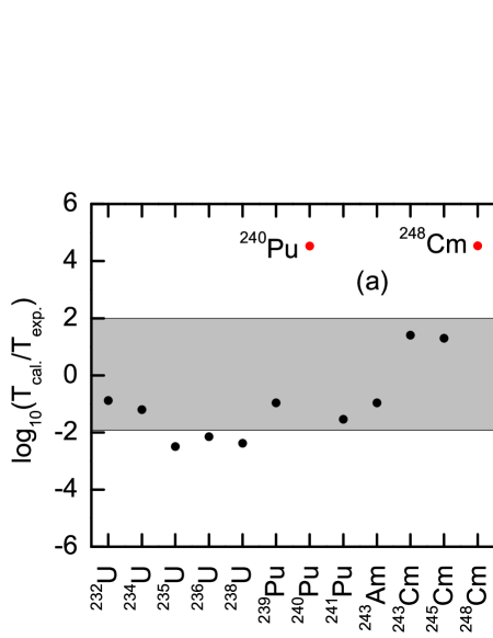
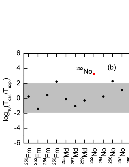
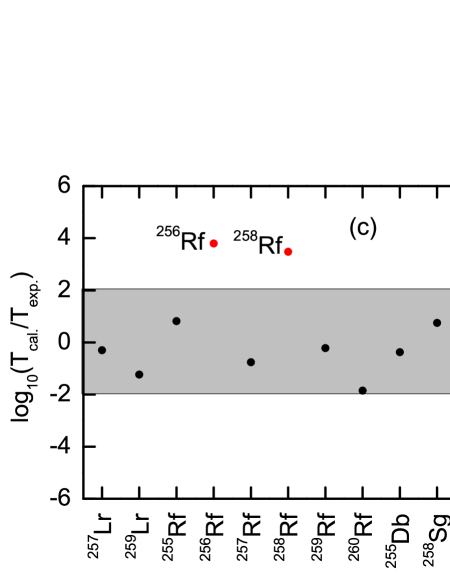
Figure 2: Deviations between the logarithms of the calculated half-lives and the experimental values for spontaneous fission from different parent nuclei.

Table 1: Comparison between experimental and theoretical spontaneous fission half-lives(the unit is seconds) of heavy and super-heavy nuclei.

Nucleus	$T_{1/2}$(exp.)	$T_{1/2}$(the.)	Nucleus	$T_{1/2}$(exp.)	$T_{1/2}$(the.)
${}_{92}^{232}$U	$2.5\times 10^{21}$	$3.3\times 10^{20}$	${}_{102}^{252}$No	$1.2\times 10^{1}$	$2.2\times 10^{4}$
${}_{92}^{234}$U	$4.7\times 10^{23}$	$2.9\times 10^{22}$	${}_{102}^{254}$No	$3.0\times 10^{4}$	$5.1\times 10^{4}$
${}_{92}^{235}$U	$3.1\times 10^{26}$	$1.0\times 10^{24}$	${}_{102}^{256}$No	$1.1\times 10^{2}$	$2.1\times 10^{4}$
${}_{92}^{236}$U	$7.8\times 10^{23}$	$5.5\times 10^{21}$	${}_{102}^{257}$No	$1.7\times 10^{3}$	$2.0\times 10^{4}$
${}_{92}^{238}$U	$2.6\times 10^{23}$	$1.1\times 10^{21}$	${}_{102}^{259}$No	$3.5\times 10^{4}$	$2.0\times 10^{3}$
${}_{94}^{239}$Pu	$2.5\times 10^{23}$	$2.7\times 10^{22}$	${}_{103}^{252}$Lr	$3.6\times 10^{1}$	$2.0\times 10^{2}$
${}_{94}^{240}$Pu	$1.5\times 10^{18}$	$5.1\times 10^{22}$	${}_{103}^{253}$Lr	$2.9\times 10^{1}$	$9.2\times 10^{2}$
${}_{94}^{241}$Pu	$2.3\times 10^{24}$	$6.6\times 10^{22}$	${}_{103}^{255}$Lr	$2.2\times 10^{4}$	$1.0\times 10^{3}$
${}_{95}^{243}$Am	$6.3\times 10^{21}$	$6.9\times 10^{20}$	${}_{103}^{256}$Lr	$9.0\times 10^{5}$	$3.3\times 10^{3}$
${}_{96}^{243}$Cm	$1.7\times 10^{19}$	$4.4\times 10^{20}$	${}_{103}^{257}$Lr	$2.2\times 10^{3}$	$1.1\times 10^{3}$
${}_{96}^{245}$Cm	$4.4\times 10^{19}$	$8.6\times 10^{20}$	${}_{103}^{259}$Lr	$5.8\times 10^{3}$	$3.4\times 10^{2}$
${}_{96}^{248}$Cm	$1.3\times 10^{14}$	$4.6\times 10^{18}$	${}_{104}^{255}$Rf	$3.2\times 10^{0}$	$2.1\times 10^{1}$
${}_{97}^{249}$Bk	$6.1\times 10^{16}$	$2.1\times 10^{16}$	${}_{104}^{256}$Rf	$6.4\times 10^{-3}$	$4.0\times 10^{1}$
${}_{98}^{249}$Cf	$2.2\times 10^{18}$	$2.5\times 10^{16}$	${}_{104}^{257}$Rf	$3.9\times 10^{2}$	$8.7\times 10^{1}$
${}_{98}^{250}$Cf	$5.2\times 10^{11}$	$4.1\times 10^{16}$	${}_{104}^{258}$Rf	$1.4\times 10^{-2}$	$4.2\times 10^{1}$
${}_{99}^{253}$Es	$2.0\times 10^{13}$	$2.6\times 10^{12}$	${}_{104}^{259}$Rf	$4.0\times 10^{1}$	$2.4\times 10^{1}$
${}_{99}^{255}$Es	$8.4\times 10^{10}$	$2.3\times 10^{8}$	${}_{104}^{260}$Rf	$5.1\times 10^{-2}$	$3.6\times 10^{0}$
${}_{100}^{250}$Fm	$2.6\times 10^{7}$	$4.5\times 10^{7}$	${}_{105}^{255}$Db	$8.0\times 10^{-1}$	$3.5\times 10^{-1}$
${}_{100}^{252}$Fm	$4.0\times 10^{9}$	$1.6\times 10^{8}$	${}_{106}^{258}$Sg	$5.2\times 10^{-3}$	$2.9\times 10^{-2}$
${}_{100}^{254}$Fm	$1.9\times 10^{7}$	$5.2\times 10^{7}$	${}_{106}^{260}$Sg	$7.2\times 10^{-3}$	$4.1\times 10^{-3}$
${}_{100}^{256}$Fm	$1.0\times 10^{4}$	$1.7\times 10^{6}$	${}_{106}^{262}$Sg	$7.0\times 10^{-3}$	$3.9\times 10^{-5}$
${}_{101}^{255}$Md	$1.1\times 10^{6}$	$8.4\times 10^{5}$	${}_{108}^{264}$Hs	$1.6\times 10^{-3}$	$5.1\times 10^{-8}$
${}_{101}^{257}$Md	$2.0\times 10^{6}$	$1.8\times 10^{5}$	${}_{114}^{286}$Fl	$1.3\times 10^{-1}$	$6.9\times 10^{-2}$
${}_{101}^{259}$Md	$5.8\times 10^{3}$	$2.9\times 10^{3}$

To illustrate the agreement between the calculations and the experimental data clearly, the comparison of the calculated spontaneous fission half-lives with the experimental data is shown in Fig.2. The absolute values of log₁₀($T_{1/2}$(cal.)/$T_{1/2}$(exp.)) are generally less than the factor 2, this means that the experimental spontaneous fission half-lives are well reproduced. Here the significant deviations between theoretical calculations and experimental data occur only for seven nuclei ²⁴⁰Pu, ²⁴⁸Cm, ²⁵⁰Cf, ²⁵²No, ²⁵⁶Rf, ²⁵⁸Rf and ²⁶⁴Hs. The deviations for the half-lives of the seven nuclei are 10⁴, 10⁴, 10⁵, 10³, 10⁴, 10³ and 10⁵. These nuclei can be separated into three classes. The first class includes ²⁴⁸Cm, ²⁵⁰Cf, ²⁵²No, ²⁵⁶Rf and ²⁵⁸Rf, and the second and three class include, respectively, ²⁶⁴Hs and ²⁴⁰Pu. For ²⁴⁸Cm, ²⁵⁰Cf, ²⁵²No, ²⁵⁶Rf and ²⁵⁸Rf the neutron numbers are near N=152. Especially, for $N=152$ isotones ²⁴⁸Cm, ²⁵⁰Cf and ²⁵⁶Rf, the deviations are a little larger. Such a large deviation seems due to the sub-magic neutron shell closure at $N=152$. To illustrate more clearly that $N=152$ is the sub-magic neutron shell closure, $\alpha$-decay half-lives have been calculated within a tunnelling effect through a potential barrier determined by the GLDM and the WKB approximation. Fig. 3 represents the plot connecting calculated $\alpha$-decay half-lives against neutron number of the even-even parent isotopes with Z ranging from 98 to 108. Two peaks appear at $N=152$ and $N=162$. In $\alpha$ and cluster emission it is found that half-life has the minimum value for those decays which lead to doubly magic daughter [37, 38, 39, 40]. Therefore the peaks at $N=152$ and $N=162$ indicate the presence of shell closures at these values. We would like to point out that many authors [41, 42, 43, 44, 45] have predicted sub-magic neutron shell closures at $N=152$ and $N=162$. The deviation for ²⁶⁴Hs seems indicate that there is a proton shell closure for $Z=108$. The macroscopic-microscopic model has predicted that ²⁷⁰Hs is a deformed doubly magic nucleus [46]. Recently, shells at $N=162$ neutrons and $Z=108$ protons were predicted by GLDM [47]. These predictions have been supported by experiments [48, 49, 50]. The spontaneous fission process is complex and there are large uncertainties existing in the fission process, so one may consider that the slightly larger deviations of $10^{4}$ for few nuclei are acceptable[54].

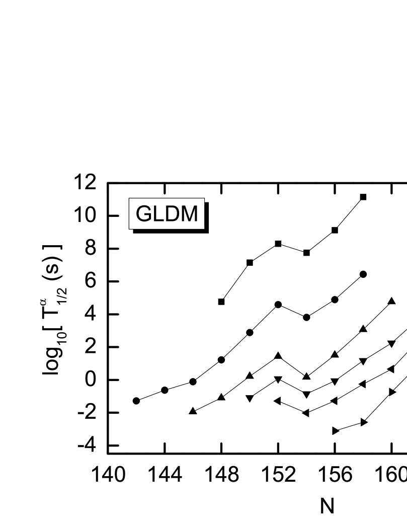
Figure 3: Theoretical half-lives versus neutron number for various parent nuclei with $Z=98-108$ emitting $\alpha$-decay.

Fig.4 represents the comparison of our spontaneous fission half-lives from ²⁵⁰Fm to ²⁶²Sg with the results from Ref.[11] and with the experimental values [36]. Solid triangles represent experimental data and solid circles denote the present calculated half-lives. Open circles show the results from Ref. [11], in which the Yukawa-plus-exponential model for the macroscopic part of the potential energy and the Strutinsky shell correction, based on the Woods-Saxon single-particle potential, for the microscopic part are employed. The trend of theoretical results from Ref.[11] follows well the experimental ones. However, these values [11] are systematical larger than the experimental ones and larger than ours by up to about six orders of magnitude. The difference seems to originate mainly from the shell corrections. In our approach the shell corrections have been introduced as defined in the Droplet Model [31] with an attenuation factor. Using this approach, shell corrections only play a role near the ground state of the compound nucleus and not at the saddle-point. It has been clearly demonstrated within a single-particle model with pairing corrections [51, 52] that, for two separated spheroids, the shell effects are strongly diminished since they are properties of valence nucleons and that the orbital of which are strongly perturbed by the nuclear proximity potential. Thus, as soon as the shape is creviced, the application of the standard shell corrections to the liquid drop model energy seems to overestimate the veritable shell effects which are partially destroyed by the proximity forces. By comparing the present results of spontaneous fission half-lives with the results from Ref. [11], we would like to point out that our calculated values better reproduce the experimental data.

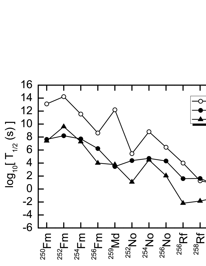
Figure 4: The comparison of the logarithm of the present spontaneous fission half-lives with the values taken from P.Möller et al [11] and the experimental data.

Fig.5 represents the comparison of our spontaneous fission half-lives for partial odd-A and odd-odd nuclei with the results from Ref. [53] and with the experimental values [36]. Solid triangles represent the calculated spontaneous fission half-lives from Ref. [53], in which the phenomenological formula for spontaneous fission half-lives is given by

$$\log_{10}(T_{1/2}/yr)=21.08+C_{1}\frac{(Z-90-\upsilon)}{A}$$ (3.35)

$$+C_{2}\frac{(Z-90-\upsilon)^{2}}{A}+C_{3}\frac{(Z-90-\upsilon)^{3}}{A}$$

$$+C_{4}\frac{(Z-90-\upsilon)(N-Z-52)^{2}}{A},$$

where C₁=-548.825021, C₂=-5.359139, C₃=0.767379 and C₄=-4.282220, the seniority term $\upsilon$ is $\upsilon$=0 for the spontaneous fission of even-even nuclei and $\upsilon$=2 for spontaneous fission of odd A and odd-odd nuclei. The value $\upsilon$ indicates the blocking effect of unpaired nucleon on the transfer of many nucleon-pairs during the fission process. The agreement between the experimental and theoretical half-lives are generally good except for a few cases (e.g. ²⁵⁹Rf and ²⁵⁵Db).

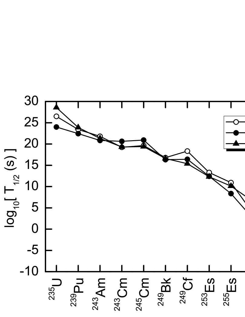
Figure 5: The comparison of the logarithm of the present spontaneous fission half-lives with the values taken from Ren et al [53] and the experimental data.

Since the present calculated half-lives agree well with the experimental ones, the calculations are extended to provide some predictions for spontaneous fission half-lives, which will be useful for future experiments to synthesize and detect the new SHN. The predictions are shown for Z=114-120 isotopic chains in Table 2. For some SHN, the spontaneous fission half-lives are long enough to be measured with the present experimental setups.

4 Summary

The spontaneous fission process in the quasimolecular shape valley is investigated within a generalized liquid drop model where the microscopic shell corrections and the phenomenological pairing corrections are considered. A systematic calculation on spontaneous fission half-lives for heavy and superheavy nuclei with proton number Z $\geq$ 92 is performed. The calculated half-lives are in good agreement with the experimental data. For most nuclei, the experimental half-lives are reproduced within a factor of $10^{2}$. This level of agreement is very satisfactory because the spontaneous fission is much more complex than other decay modes such as cluster radioactivities and $\alpha$-decay. Spontaneous fission half-lives of the isotopes of $Z=114-120$ are predicted, presuming that this might help to discriminate between all the possible future experiments.

Table 2: Predicted half-lives (the unit is seconds) of spontaneous fission of even-even nuclei on Z=114-120 isotopic chain.

Nucleus	$T_{1/2}$(cal.)	Nucleus	$T_{1/2}$(cal.)	Nucleus	$T_{1/2}$(cal.)	Nucleus	$T_{1/2}$(cal.)
${}^{280}Fl$	$2.2\times 10^{-3}$	${}^{282}Fl$	$2.0\times 10^{-1}$	${}^{284}Fl$	$1.2\times 10^{-1}$	${}^{288}Fl$	$1.1\times 10^{0}$
${}^{290}Fl$	$2.3\times 10^{3}$	${}^{292}Fl$	$6.9\times 10^{7}$	${}^{294}Fl$	$3.6\times 10^{8}$	${}^{296}Fl$	$3.3\times 10^{8}$
${}^{300}Fl$	$2.6\times 10^{-1}$	${}^{286}Lv$	$1.4\times 10^{-5}$	${}^{288}Lv$	$2.0\times 10^{-5}$	${}^{290}Lv$	$2.5\times 10^{-3}$
${}^{292}Lv$	$5.5\times 10^{0}$	${}^{294}Lv$	$1.1\times 10^{5}$	${}^{296}Lv$	$2.7\times 10^{5}$	${}^{298}Lv$	$8.8\times 10^{3}$
${}^{300}Lv$	$1.1\times 10^{4}$	${}^{302}Lv$	$2.6\times 10^{-5}$	${}^{292}118$	$1.4\times 10^{-4}$	${}^{294}118$	$2.2\times 10^{-1}$
${}^{296}118$	$3.9\times 10^{3}$	${}^{298}118$	$1.4\times 10^{2}$	${}^{300}118$	$2.8\times 10^{1}$	${}^{302}118$	$6.9\times 10^{1}$
${}^{294}120$	$6.3\times 10^{-5}$	${}^{296}116$	$8.6\times 10^{-2}$	${}^{298}120$	$1.1\times 10^{1}$	${}^{300}120$	$1.0\times 10^{1}$
${}^{302}120$	$2.3\times 10^{1}$	${}^{304}120$	$3.1\times 10^{1}$	${}^{306}120$	$3.0\times 10^{-6}$

References

- [1] N. Bohr and J.A. Wheeler, Phys. Rev. 56 (1939) 426.
- [2] G.N. Flerov and K.A. Petrzak, Phys. Rev. 58 (1940) 89.
- [3] N.E. Holden and D.C. Hoffman, Pure Appl. Chem. 72 (2000) 1525.
- [4] W.J. Swiatecki, Phys. Rev. 100 (1955) 937.
- [5] V.M. Strutinsky, Nucl. Phys. A 95 (1967) 420.
- [6] V.M. Strutinsky, Nucl. Phys. A 122 (1968) 1.
- [7] P. Möller, D.G. Madland, A.J. Sierk, and A. Iwamoto, Nature 409 (2001) 785.
- [8] P. Möller, A.J. Sierk, T. Ichikawa, A. Iwamoto, R. Bengtsson, H. Uhrenholt, and S. Åberg, Phys. Rev. C 79 (2009) 064304.
- [9] A. Sobiczewski and K. Pomorski, Prog. Part. Nucl. Phys. 58 (2007) 292.
- [10] P. Möller, J.R. Nix, and W.J. Swiatecki, Nucl. Phys. A 469 (1987) 1.
- [11] P. Möller, J.R. Nix, and W.J. Swiatecki, Nucl. Phys. A 492 (1989) 349.
- [12] K.E. Gregorich et al., Phys. Rev. C 74 (2006) 044611.
- [13] J. Dvorak et al., Phys. Rev. Lett. 97 (2006) 242501.
- [14] D. Peterson et al., Phys. Rev. C 74 (2006) 014316.
- [15] Yu. Ts. Oganessian et al., Phys. Rev. C 72 (2005) 034611.
- [16] Yu. Ts. Oganessian et al., Phys. Rev. C 74 (2006) 044602.
- [17] Yu. Ts. Oganessian et al., Phys. Rev. C 70 (2004) 064609.
- [18] G. Royer and B. Remaud, J. Phys. G: Nucl. Part. Phys. 10 (1984) 1541.
- [19] G. Royer and F. Haddad, Phys. Rev. C 51 (1995) 2813.
- [20] G. Royer and K. Zbiri, Nucl. Phys. A 697 (2002) 630.
- [21] C. Bonilla and G. Royer, Acta Phys. Hung. A 25 (2006) 11.
- [22] G. Royer, J. Phys. G: Nucl. Part. Phys. 26 (2000) 1149.
- [23] H.F. Zhang, W. Zuo, J.Q. Li, and G. Royer, Phys. Rev. C 74 (2006) 017304.
- [24] G. Royer and H.F. Zhang, Phys. Rev. C 77 (2008) 037602.
- [25] H.F. Zhang and G. Royer, Phys. Rev. C 77 (2008) 054318.
- [26] G. Royer and R. Moustabchir, Nucl. Phys. A 683 (2001) 182.
- [27] G. Royer, B. Remaud, Nucl. Phys. A 444 (1985) 477.
- [28] G. Royer and B. Remaud, J. Phys. G: Nucl. Part. Phys. 8 (1982) L159.
- [29] J. Blocki, J. Randrup, W.J. Swiatecki, C.F. Tsang, Annals of Physics 105 (1977) 427.
- [30] G. Royer and C. Piller, J. Phys. G: Nucl. Part. Phys. 18 (1992) 1805.
- [31] W.D. Myers, Droplet Model of Atomic Nuclei (Plenum, New-York, 1977).
- [32] Ning Wang, Min Liu and Xizhen Wu, Phys. Rev. C 81 (2010) 044322.
- [33] Ning Wang and Min Liu, Phys Rev C 81 (2010) 067302.
- [34] P. Möller, J.R. Nix, W.D. Myers and W.J. Swiatecki, Atom. Data Nucl. Data Tabl. 59 (1995) 185.
- [35] J. Randrup, S.E. Larsson, P. Möller, S.G. Nilsson, K. Pomorski and A. Sobiczewski, Phys. Rev. C 13 (1976) 229.
- [36] J. Tuli et al, Nuclear Wallet cards, Brookhaven National Laboratory (2000).
- [37] R.K. Gupta and W. Greiner, Int. J. Mod. Phys. E 3 (1994) 335.
- [38] D.N. Poenaru, R.A. Gherghescu, and W. Greiner, Phys. Rev. Lett. 107 (2011) 062503; Phys. Rev. C 85 (2012) 034615.
- [39] C. Qi, F.R. Xu, R.J. Liotta, and R. Wyss, Phys. Rev. Lett. 103 (2009) 072501.
- [40] A. Sobiczewski, Radiochim. Acta 99 (2011) 395.
- [41] P. Möller, J.R. Nix, J. Phys. G: Nucl. Part. Phys. 20 (1994) 1681.
- [42] R. Smolańczuk, J. Skalski, and A. Sobiczewski Phys. Rev. C 52 (1995) 4.
- [43] G.A. Lalazissis, M.M. Sharma, P. Ring, Y.K. Gambhir, Nucl. Phys. A 608 (1996) 202.
- [44] L. Satpathy, arXiv:nucl-th/0105064v1, 2001.
- [45] D.N. Poenaru, I.H. Plonski, W. Greiner, Phys. Rev. C 74 (2006) 014312.
- [46] Z. Patyk, A. Sobiczewski, and S. Cwiok, Nucl. Phys. A 502 (1989) 591.
- [47] H.F. Zhang, Y. Gao, N. Wang, J.Q. Li, E.G. Zhao, and G. Royer, Phys. Rev. C 85 (2012) 014325.
- [48] Yu.A. Lazarev et al., Phys. Rev. Lett. 73 (1994) 624.
- [49] Yu.A. Lazarev et al., Phys. Rev. Lett. 75 (1995) 1903.
- [50] J. Dvorak et al., Phys. Rev. Lett. 97 (2006) 242501.
- [51] W. Nörenberg, Phys. Lett. B 31 (1970) 621.
- [52] W. Nörenberg, Phys. Rev. C 5 (1972) 2020.
- [53] Z. Ren and C. Xu, Nucl. Phys. A 759 (2005) 64; C. Xu, Z. Ren, and Y. Guo, Phys. Rev. C 78 (2008) 044329.
- [54] K. P. Santhosh, R. K. Biju and Sabina Sahadevan, J. Phys. G: Nucl. Part. Phys. 39 (2009) 115101; Nucl. Phys. A 832 (2010) 220.