Using Artificial Intelligence Models in System Identification

by

Wesam Samy Mohammed Elshamy

A Thesis Submitted to the

Faculty of Engineering at Cairo University

in Partial Fulfillment of the

Requirements for the Degree of

Master of Science
in

Electrical Power and Machines

Under the Supervision of

Dr. Ahmed Bahgat Gamal Bahgat

Professor, Department of Electrical Power and Machines

Dr. Hassan Mohammed Rashad

Assoc. Professor, Department of Electrical Power and Machines

Faculty of Engineering, Cairo University
Giza, Egypt
22 May 2007

Abstract

Artificial Intelligence (AI) techniques are known for its ability in tackling problems found to be unyielding to traditional mathematical methods. A recent addition to these techniques are the Computational Intelligence (CI) techniques which, in most cases, are nature or biologically inspired techniques. Different CI techniques found their way to many control engineering applications, including system identification, and the results obtained by many researchers were encouraging. However, most control engineers and researchers used the basic CI models as is or slightly modified them to match their needs. Henceforth, the merits of one model over the other was not clear, and full potential of these models was not exploited.

In this research, Genetic Algorithm (GA) and Particle Swarm Optimization (PSO) methods, which are different CI techniques, are modified to best suit the multimodal problem of system identification. In the first case of GA, an extension to the basic algorithm, which is inspired from nature as well, was deployed by introducing redundant genetic material. This extension, which come in handy in living organisms, did not result in significant performance improvement to the basic algorithm. In the second case, the Clubs-based PSO (C-PSO) dynamic neighborhood structure was introduced to replace the basic static structure used in canonical PSO algorithms. This modification of the neighborhood structure resulted in significant performance of the algorithm regarding convergence speed, and equipped it with a tool to handle multimodal problems.

To understand the suitability of different GA and PSO techniques in the problem of system identification, they were used in an induction motor’s parameter identification problem. The results enforced previous conclusions and showed the superiority of PSO in general over the GA in such a multimodal problem. In addition, the C-PSO topology used significantly outperformed the two other static topologies in all performance measures used in this problem.

Acronyms

ACO

Ant Colony Optimization

AI

Artificial Intelligence

ANN

Artificial Neural Network

ARMA

Auto-Regressive Moving Average

CI

Computational Intelligence

C-PSO

Clubs-based PSO

DAS

Dominant-alleles-set

DM

Decision Maker

EA

Evolutionary Algorithm

EC

Evolutionary Computation

EMO

Evolutionary Multi-objective Optimization

EP

Evolutionary Programming

ES

Evolutionary Strategies

FDR-PSO

Fitness-Distance-Ratio PSO

FIPS

Fully Informed Particle Swarm

FPS

Fitness Proportionate Selection

GA

Genetic Algorithm

GP

Genetic Programming

H-PSO

Hierarchical PSO

LCS

Learning Classifier Systems

LQG

Linear Quadratic Gaussian

LS

Line Search

MOEA

Multi-Objective Evolutionary Algorithm

MLP

Multi-Layered Perceptron

MOP

Multiobjective Optimization Problem

NARMAX

Non-linear Auto-Regressive Moving Average model with eXogenous inputs

NFL

No Free Lunch

NSGA-II

Non-dominated Sorting Genetic Algorithm II

PF

Pareto-optimal Front

PID

Proportional-Integral-Derivative

PSO

Particle Swarm Optimization

RBF

Radial Basis Function

RMS

Root-Mean-Square

SAE

Sum of Absolute Error

SD

Steepest Descent

SDS

Stochastic Diffusion Search

SI

Swarm Intelligence

SOP

Single-objective Optimization Problem

SAT

Boolean Satisfiability Problem

SBX

Simulated Binary Crossover

TSP

Traveling Salesman Problem

Chapter 1 Introduction

1.1 Motivation

The field of AI inevitably emerged as computers started to find their way in many applications. Engineers and computer scientists who worked on developing AI models, started using these models to solve many problems they faced. The success of many AI applications in computer science and computer engineering were exciting, it became possible to find the meaning of a word according to its context, computers and machines became able to understand spoken language to some extent, and recently were used to match fingerprints. Until recently, many of the AI models were developed to solve problems in computer engineering and computer science in the first place. These models were later used as is or slightly modified by researchers in other fields.

Control engineers and researchers were enthusiastic about the results obtained by their fellows in the computer science field. They were scrutinizing the AI models developed by their fellows because back in their labs, they faced complex problems unyielding to traditional mathematical techniques. Among these problems is the system identification problem. The problem of system identification with its hard nonlinearity, multimodality, and constraints is especially unsuitable for traditional mathematical techniques, and the results obtained using these techniques are unsatisfactory for most real life applications. Henceforth, control engineers started using the models developed by their fellows to solve system identification problems. The results obtained were encouraging, and many AI models became the method of choice for many control engineers.

The author of this thesis belongs to both groups of researchers. He was unsatisfied by the off-the-shelf AI models used by control engineers, so he used his knowledge in both fields to test, modify, and develop new models with the problem of system identification in mind.

A new wave of AI models is the CI techniques, which are in most cases, are nature inspired, or biologically inspired techniques. Recent research have shown promising results in their applications in many control engineering problems, and specifically, system identification problems [1]. Due to their inherent capability of handling many of the difficulties encountered in control engineering problems, and because of the encouraging results reported by many researchers, it was found by the author of this thesis that developing these techniques is the next logical step to pursue.

1.2 Thesis Outline

After this brief introduction, the optimization problem with its various types is presented in Chapter 2. After the Single and Multiobjective problems are presented and their terminology and definitions are explained in Section 2.1 and 2.2, respectively, the difficulties faced in solving these problems are detailed in Section 2.3.

The thesis moves to non-traditional techniques by presenting the Evolutionary Algorithms (EAs) in Chapter 3. After an introduction in Section 3.1, the logic behind Evolutionary Algorithms and an analysis of their behavior is detailed in Section 3.2, and an example of these techniques, which is the GAs, presented in detail in Section 3.3. Finally, a proposed extension to the GA model is explained, tested on a set of benchmark problems, and a conclusion about its efficiency is given in Section 3.4.

More CI models follow in Chapter 4 where the Swarm Intelligence (SI) methods are presented. The chapter starts by an introduction then explains some theoretical aspects about these techniques in Section 4.2. An example of the SI techniques which is the PSO is presented followed by some of its variations in Section 4.3 and 4.4, respectively. A proposed modification to some aspects of the PSO model is explained, analyzed, tested on many test problems, and the results were furnished and followed by a conclusion in Section 4.5. Finally, a comparison between the GA and PSO models concludes the chapter.

Chapter 5 is concerned about the applications of CI techniques in control engineering, and particularly in system identification. It starts by outlining the advantages and disadvantages of using CI methods in control engineering in Section 5.1 and 5.2, respectively. Different applications in control engineering are presented in Section 5.3 and the problem of system identification is given in more detail in Section 5.4. The problem of parameter identification of an induction motor is explained, its model is driven, the algorithms used to solve it are presented, and the experiment is carried out with its results explained and a conclusion is furnished in Section 5.5.

Chapter 6 concludes this thesis by analyzing the results reached in previous chapters and proposes future research directions.

Chapter 2 The Optimization Problem

The Optimization Problem is encountered in every day life. A man driving to work usually chooses a route that minimizes his travel time. An investor makes many decisions on daily basis to minimize his business risks and increase his profits. Even electrons tend to occupy the lowest energy level available [2]. The problem of optimization becomes a matter of life or death in some situations. A bad utilization of energy or food reserves of a nation may lead to crises and loss of life.

The Optimization Problem could be as simple as shopping for a good looking shirt with a reasonable price, or as complicated as scheduling air flights for a major airline company. Although those two examples are at the extremes, they do have the characteristics of the optimization problem. Both of them have objectives; the objectives of the first problem is to find and buy a shirt that looks as good as possible and is as cheap as possible, while for the second problem the objective is to increase profits as much as possible. Each one of those problems has parameters or decision variables which by tuning them properly the objectives are optimized. For the first problem these parameters include the shop location, brand name and shirt fabric etc., while for the second problem these parameters include flight destinations, ticket prices, pilots and crew salaries and flights schedule among many others. Figure 2.2 shows the mapping between the decision space, which contains the parameters, and the objective space. Based on this mapping, the Decision Maker (DM) chooses the parameters, which make-up the decision vector, that maps to the desired point in the objective space. Neither the decision space nor the objective space has to be continuous or connected. Optimization problems can be classified into two categories regarding the number of objectives; i) Single-objective Optimization Problemsand ii) Multiobjective Optimization Problems

2.1 Single-objective Optimization Problems

Single-objective Optimization Problems, as their name implies, are problems that have single objective to be optimized (maximized or minimized) by varying their parameters. A SOP can be defined as follows [3, 4]:

Definition 1 (Single-objective Optimization Problem).

optimize $$y=f(\text{\bf x})\in\text{\bf Y}$$ (2.1)

$$s.t.\quad h_{i}(\text{\bf x})=0\quad i=1,2\dotsc m$$ (2.2)

$$g_{j}(\text{\bf x})\geq 0\quad j=1,2,\dotsc l$$ (2.3)

$$\text{\bf x}=[x_{1}\dotsm x_{n}]^{T}\in\text{\bf X}$$ (2.4)

where $x_{i}$ is a decision variable, x is a decision vector, X is the decision space, $y$ is an objective function, Y is the objective space and $h_{i}(\text{\bf x})$ and $g_{j}(\text{\bf x})$ are equality and inequality constraint functions respectively.

The constraint functions determine the feasible set.

Definition 2 (Feasible Set).

The feasible set $\text{\bf X}_{f}$ is the set of decision vectors x that satisfy the constraints $h_{i}(\text{\bf x})$ and $g_{j}(\text{\bf x})$.
The image of the feasible set in the objective space is known as the feasible region.

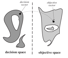
Figure 2.1: Decision space—objective space mapping

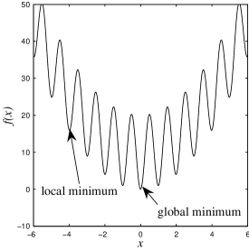
Figure 2.2: Landscape of Rastrigin problem ($n=1$)

A well known SOP is the Rastrigin test problem [5, 6]. It is defined as follows:

minimize $$f(\text{\bf x})=\sum_{i=1}^{n}\left[x_{i}^{2}-10\cos(2\pi x_{i})+10\right]$$ (2.5)

s.t. $$\text{\bf x}\in[-6,6]^{n}$$ (2.6)

where $n$ is the number of decision variables. Figure 2.2 shows the landscape of this problem for $n=1$. The minimum value of the objective function in the feasible region is achieved at the global minimum, or more generally, the global optimum.

Definition 3 (Global Optimum).

A global optimum is a point in the feasible region whose value is better than all other points in that region

For the Rastrigin problem shown in Figure 2.2 the global minimum is achieved at $x=0$ with a value of $f(\text{\bf x})=0$. Excluding the valley where the global minimum lies at its bottom, there are 12 valleys in this problem’s landscape. The point at the bottom of each one of them is known as a local minimum, or more generally, a local optimum.

Definition 4 (Local Optimum).

A local optimum is a point in the feasible region whose value is better than all other points in its vicinity in the region, and is worse than the global optimum.

2.2 Multiobjective Optimization Problems

Unlike SOPs, MOPs have many objectives to be optimized concurrently, and most of the time these objectives are conflicting. A MOP can be defined as follows [3, 4]:

Definition 5 (Multiobjective Optimization Problem).

optimize $$\text{\bf y}=\text{\bf F}(\text{\bf x})=\{f_{1}(\text{\bf x}),f_{2}(\text{\bf x}),\dotsc,f_{k}(\text{\bf x})\}\in\text{\bf Y}$$ (2.7)

$$s.t.\quad \text{\bf x}\in\text{\bf X}$$ (2.8)

$$\text{\bf X}=\left\{\;\text{\bf x}\left|\begin{aligned} &h_{i}(\text{\bf x})=0\quad i=1,\dotsc m\\ &g_{j}(\text{\bf x})\leq 0\quad j=1,\dotsc l\\ &\text{\bf x}=[x_{1}\dotsm x_{n}]^{T}\end{aligned}\right.\right\}$$ (2.9)

where $x_{i}$ is a decision variable, x is a decision vector, X is the decision space, y is a vector of $k$ objective functions, Y is the objective space and $h_{i}(\text{\bf x})$ and $g_{j}(\text{\bf x})$ are equality and inequality constraint functions respectively.

This definition can be illustrated using the following classic example [7, 8]:

minimize $$\text{\bf F}(\text{\bf x})=\{f_{1}(\text{\bf x}),f_{2}(\text{\bf x})\},\quad\text{where}$$ (2.10)

$$f_{1}(\text{\bf x})=x^{2}$$ (2.11)

$$f_{2}(\text{\bf x})=(x-2)^{2}$$ (2.12)

Figure 2.4 shows the values of the objective functions $f_{1}$ and $f_{2}$ while varying the decision variable $x$ value. $f_{1}$ and $f_{2}$ are monotonically decreasing with $x$ in the range $x\in(-\infty,0)$, so the two objectives are in harmony [9], which means that an improvement in one of them is rewarded with simultaneous improvement in the other. The higher the value of $x$ in this range the better (the lower) the value of the two objectives become. A similar situation happens in the range $x\in(2,\infty)$. The two objective functions are in harmony and monotonically decreasing with $x$ in this range; the smallest possible value of $x$ in this range is translated to the best (the lowest) value for the two objectives in that range. However, The two objectives are in conflict in the range $x\in[0,2]$; An increase in $x$ value is accompanied by improvement of $f_{1}$ and deterioration of $f_{2}$.

A mapping of Figure 2.4 to the objective space gives Figure 2.4. The regions $x\in(-\infty~{}0)$, $x\in[0~{}2]$ and $x\in(2~{}\infty)$ in Figure 2.4 are mapped to the upper-left dashed segment, solid segment and the lower-right dashed segment in Figure 2.4 respectively. It is clear that points d, e and f are in the harmony region, while points a, b and c are in the conflict region.

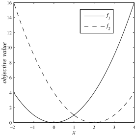
Figure 2.3: Decision parameter’s value against Objectives’ values

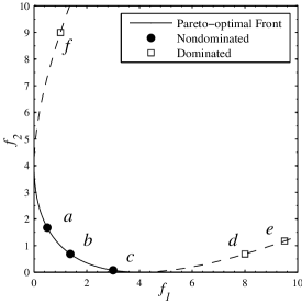
Figure 2.4: Objective space of a MOP

Using logical comparison, the following relationships are established: Objective vector b is better than objective vector d because although they have the same $f_{2}$ value, b has a lower $f_{1}$ value. Objective vector c is better than objective vector d as well; it has lower $f_{1}$ and $f_{2}$ values. The following definition is used to put these relationships in mathematical notation [4].

Definition 6.

For any two objective vectors $\boldsymbol{u}$ and $\boldsymbol{v}$,

u $$=\text{\bf v} \forall i\in\{1,2,\dotsc,k\}: u_{i}=v_{i}$$ iff (2.13)

u $$\leq\text{\bf v} \forall i\in\{1,2,\dotsc,k\}: u_{i}\leq v_{i}$$ iff (2.14)

u $$<\text{\bf v} \text{\bf u}\leq\text{\bf v}\wedge\text{\bf u}\neq\text{\bf v}$$ iff (2.15)

In a minimization SOP, a solution r is better than a solution s, iff $p(\text{\bf r})<p(\text{\bf s})$, where $p$ is the objective function. But in a MOP this comparison mechanism does not hold because there are more than one objective to be concurrently optimized. In Figure 2.4, $c<d$ and $c\nless a$, but $a\nless d$. This may seem illogical when using SOPs reasoning, but in MOPs this situation is quite common. The points $a$ and $c$ represent two different solutions yet none of them is superior to the other; although the solution represented by $a$ has lower $f_{1}$ value than that of $c$, the solution represented by $c$ has lower $f_{2}$ value than that of $a$. This means that a new relationship is needed to compare two different decision vectors a and b in a MOP when $\text{\bf F}(\text{\bf a})\nleq\text{\bf F}(\text{\bf b})\wedge\text{\bf F}(\text{\bf b})\nleq\text{\bf F}(\text{\bf a})$. This relationship is described using Pareto Dominance [4, 10, 11].

Definition 7 (Pareto Dominance).

For any two decision vectors a and b in a minimization problem without loss of generality,

a $$\prec\text{\bf b} (\text{\bf a}\text{\emph{ dominates }}\text{\bf b}) \text{\bf F}(\text{\bf a})<\text{\bf F}(\text{\bf b})$$ iff (2.16)

a $$\preceq\text{\bf b} (\text{\bf a}\text{\emph{ weakly dominates }}\text{\bf b}) \text{\bf F}(\text{\bf a})\leq\text{\bf F}(\text{\bf b})$$ iff (2.17)

a $$\sim\text{\bf b} (\text{\bf a}\text{\emph{ is indifferent to }}\text{\bf b}) \text{\bf F}(\text{\bf a})\nleq\text{\bf F}(\text{\bf b})\wedge\text{\bf F}(\text{\bf b})\nleq\text{\bf F}(\text{\bf a})$$ iff (2.18)

Pareto Dominance is attributed to the Italian sociologist, economist and philosopher Vilfredo Pareto (1848–1923) [12]. It is used to compare the partially ordered solutions of MOPs, compared to the completely ordered solutions of SOPs. Using Pareto dominance to compare solutions represented in Figure 2.4, the following relationships are established; b dominates d because they have the same $f_{2}$ value, and b has a lower $f_{1}$ value, while b is indifferent to a because although b has a lower $f_{2}$ value, a has a lower $f_{1}$ value. The solutions represented by a, b and c are known as Pareto Optimal solutions. These solutions are optimal in the sense that none of their objectives can be improved without simultaneously degrading another objective.

Definition 8 (Pareto Optimality).

A decision vector $\text{\bf x}\in\text{\bf X}_{f}$ is said to be nondominated regarding a set $\text{\bf A}\subseteq\text{\bf X}_{f}$ iff

$$\nexists\>\text{\bf a}\in\text{\bf A}:\text{\bf a}\prec\text{\bf x}$$ (2.19)

If it is clear within the context which set A is meant, it is simply left out. Moreover, x is said to be Pareto optimal iff x is nondominated regarding $\text{\bf X}_{f}$

By applying this definition to the example presented in Figure 2.4. It is clear that the solutions represented by $d$, $e$ and $f$ are dominated, while $a$, $b$ and $c$ are nondominated. The set of all Pareto-optimal solutions is known as the Pareto-optimal set, and its image in the objective space is known as the Pareto-optimal Front (PF).

Definition 9 (Nondominated Sets and Fronts).

Let $\text{\bf x}\subseteq\text{\bf X}_{f}$. The function $p(\text{\bf A})$ gives the set of nondominated decision vectors in A:

$$p(\text{\bf A})=\{\text{\bf a}\in\text{\bf A}|\text{\bf a}\text{ is nondominated regarding }\text{\bf A}\}$$ (2.20)

The set $p(\text{\bf A})$ is the nondominated set regarding A, the corresponding set of objective vectors $\text{\bf f}(p(\text{\bf A}))$ is the nondominated front regarding A. Furthermore, the set $\text{\bf X}_{p}=p(\text{\bf X}_{f})$ is called the Pareto-optimal set and the set $\text{\bf Y}_{p}=\text{\bf f}(\text{\bf X}_{p})$ is denoted as the Pareto-optimal front.

The Pareto-optimal set of the example given in Equations (2.10)–(2.12) is $x\in[0~{}2]$, and its corresponding image in the objective space is the PF shown as a solid segment in Figure 2.4.

To further explain the Pareto dominance relationships, the example in Figure 2.5 is given where the two objectives $f_{1}$ and $f_{2}$ are to be minimized. The relationships given in this example show how the solution vector represented by the point $a$ at position (8,8) is seen by the other solution vectors. So, the objective space is divided by a vertical and a horizontal lines passing through point $a$ into four regions.

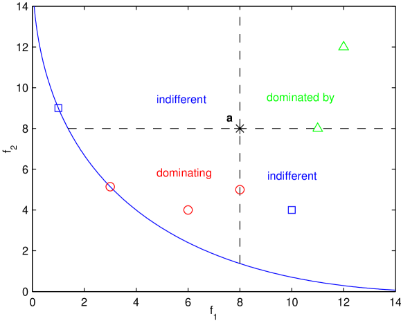
Figure 2.5: Pareto dominance relationships

• All the points in the first region at the northeast of point $a$ (including the borderlines) have higher $f_{1}$ or $f_{2}$ values, or both, so point $a$ is better than them and these points are dominated by point $a$.

• All the points in the second and fourth regions at the southeast and northwest of point $a$ (excluding the borderlines) have lower values of one objective and higher values for the other objective compared to the objective values of point $a$. So, All the points in these two regions are indifferent to point $a$. Note that although the point at position (1,9) is on the Pareto front while point $a$ is far from that front, they are indifferent to each other.

• All the points on the third region at the southwest of point $a$ (including the borderlines) have lower $f_{1}$ or $f_{2}$ values, or both. Which means that they are better than point $a$ and they are dominating point $a$.

2.3 Difficulties in Optimization Problems

A researcher or a problem solver could easily be overwhelmed by the great number of algorithms found in literature dealing with optimization. Some of them dated back to 1600 BC [13], while others are being developed as this text is being typed. These myriads of algorithms are developed to deal with different types of difficulties in optimization problems. The performance of each these optimizers depends on the characteristics of the problem it optimizes such as being linear/nonlinear, static/dynamic, SOP/MOP, combinatorial/discrete/continuous, types and number of constraints, size of the search space…etc. According to the No Free Lunch (NFL) theorems [14], all algorithms perform exactly the same when averaged over all possible problems. So, as much as possible knowledge about the problem should be incorporated in selecting the problem optimizer, because, according to NFL theorems, there is no such algorithm that will perform better than all other algorithms on all possible problems. The first step in understanding optimization problems’ characteristics is to answer the question: Why are some problems difficult to solve?[15, 16, 17, 18, 19, 20, 21, 22, 23, 24, 25]

2.3.1 The Search Space

The search space of a problem is the set of all possible solutions to that problem. To tune a radio set to a station, a reasonable man may work out an exhaustive search by scanning the entire available bandwidth in his set, but this reasonable man will never resort to exhaustive search to find the best medication for his heart, or to look up a word in a dictionary; For the medication case, the penalty of trying-out all possibilities is too high, it may lead to certain death, while exhaustively looking up a word in a dictionary takes a lot of time. To imagine how exhaustive search can easily be a laborious task, the following example is given.

A classic and one of the most used combinatorial optimization problems in AI literature is the Boolean Satisfiability Problem (SAT) [26]. The problem is to make a compound statement of boolean variables evaluate to TRUE [15]. For example, find the truth assignment for the variables $[x_{1},x_{2},\cdots,x_{100}]$ that evaluate the following function to TRUE:

$$F(\text{\bf x})=(x_{12}\lor\overline{x}_{3}\lor x_{59})\land(\overline{x}_{73}\lor x_{28}\lor\overline{x}_{9})\land\dotsm\land(\overline{x}_{69}\lor x_{92}\lor x_{5})$$ (2.21)

where $\overline{x}_{i}$ is the complement of $x_{i}$. In real world situations, such a function with 100 variables is a reasonable one, yet its search space is extremely huge; There are $2^{100}$ possible solutions for this problem. Given a computer that can test 1000 solutions of this problem per second, and that it has started its trials at the beginning of time itself, 15 billion years ago, it would have examined less than one percent of all possibilities by now [15].

The SAT problem is a combinatorial optimization problem, which means that its search space contains a finite set of solutions, and a problem solver can theoretically test all of them. But the Rastrigin problem given earlier in this chapter is a problem with a continuous search space, which means there are an infinite number of possible solutions, there is no way to test them all.

Because most people are not willing to wait for a computer to exhaustively search for a solution to the given SAT problem, other search techniques have been devised to facilitate the search task. For the radio tuning example given earlier, one can make use of the feedback sound he gets from the radio to narrow down the search space and fine-tune the set. But for the given SAT problem this mechanism is useless because the feedback, which is the value of $F(\text{\bf x})$, is always FALSE except for a single solution resulting in TRUE output. Such problems are known as needle in a haystack problems [17] as shown in Figure 2.6, where $f(x)$ equals zero in the range $x\in[-6,6]$ except for a single solution ($x=0$) where $f(x)=1$.

The landscape of the problem could be more difficult than the needle in a haystack case. It could be a misleading or deceptive landscape [27, 28, 29, 30]. In this situation the feedback (fitness value) drives the problem solver away from the global minimum, as shown in Figure 2.6. While searching this landscape for the global minimum, a higher value of $x$ is rewarded by a lower value of $f(x)$ when $x>0$, and a lower value of $x$ is rewarded by a lower value of $f(x)$ when $x<0$. This reward encourages the problem solver to move away from the global minimum at $x=0$

Another type of difficulty regarding the search space is the landscape multimodality [31, 29, 32] or ruggedness [33, 34]. A rugged landscape may trap the problem solver in a local minimum, as shown in Figure 2.6. For this minimization problem, a problem solver can easily get trapped in any of the local minima, and the odds are high that it will fall in another one if it managed to escape the first.

Figure 2.6: Landscapes of different optimization problems

2.3.2 Modeling the Problem

The fist step in solving an optimization problem is building a model for it. After this step, the real problem is put aside and the problem solver becomes concerned with the model not the problem itself. So a solution of an optimization problem is a solution to its model [15], and an optimal solution to inaccurate model, is a right solution to the wrong problem. Inaccuracies arise from wrong assumptions and simplifications.

For example, a major airline company is deciding on its carriers destinations, flights schedule and pricing policy. In this complicated task, the company may assume that customers in Brazil and Argentina are willing to pay the same price for the same service because they have similar average national income. But this assumption is wrong because customers in Argentina enjoy a high quality flights with a competitive price on their national airline company. After the company has considered all factors to build a model for their problem, its highly likely that this model will be extremely complicated to be solved by most optimization tools. So the company is faced with one of two possibilities [15].

1. Find a precise solution to a simplified version of the model.

2. Find an approximate solution to the precise model.

The first method uses traditional optimization techniques, such as linear or dynamic programming, to find a solution to the approximate model. while the second method uses non-traditional techniques, such as EAs, PSO and Ant Colony Optimization (ACO), to find an approximate solution to the precise model.

2.3.3 Constraints

Another source of difficulty in optimization problems is the constraints imposed on the problem. At first glance, these constraints may be seen as an aid to the problem solver because they do limit the search space. But in many cases they become a major source of headache and make it hard to find a single feasible solution, let alone an optimal one. The following example borrowed from [15] is used for illustration:

A common problem found in all universities is making a timetable for classes offered to students each semester. The first step in solving this problem is collecting the required data, which includes, courses offered and students registered for them, professors teaching these courses and their assistances, tools required for instruction such as projectors, computers and special blackboards, available laboratories …etc. The next step is to define the hard constraints, which are constraints that must all be met by a solution to be a feasible solution. These constraints may include:

• Every class must be assigned to an available room that has enough seats for all students and has all the tools required for students to carry experiments if any, and all special instruction tools.

• Students enrolled in more than one course must not have their courses held at the same time.

• Professors must not have two classes with overlapping time.

• Classes must not start by 8 a.m. and must not end after 10 p.m.

• Classes for the Fall semester must not start by September $1^{\text{st}}$ and must not end after December $31^{\text{st}}$.

These constraints are hard in the sense that violating them will severely hinder the education process. However in addition to these hard constraints, there are soft constraints which a solution that violates any, some or even all of them would still be feasible, but it’s highly encouraged to satisfy them. These constraints may include:

• Its preferable that undergraduate classes be held from 8 a.m. to 4 p.m., while postgraduate classes be held from 4 p.m. to 9 p.m.

• Its preferable that lectures be held before their corresponding exercise classes.

• Its preferable that students have more than 3 classes and less than 9 classes per day.

• Its desirable not to roam students across opposite ends of the campus to take their classes.

• Its preferable not to assign more than 5 classes for each professor per day.

Although these constraints are all soft constraints, some of them are more important than others. For example, its more important not to hold an exercise class before its corresponding lecture than having to make students go to opposite ends of campus. To achieve this, each constraint is assigned a weight that reflects its importance and acts as a penalty in the fitness function.

After all the constraints have been defined, the problem of finding a solution that meets all the hard constraints and optimizes the soft constraints becomes a challenging task indeed.

2.3.4 Change Over Time

Almost all real-world problems are dynamic problems, they change over time. The only thing fixed about them is the fact that they are in continuous change. A man neglecting this fact is like a stock exchange investor who assumes that share prices will remain fixed or a man who assumes that the weather will always be perfect for a picnic. To illustrate the significance of change over time, the stock investor example will be further extended.

Kevin is a stock exchange investor who must realize that the stock market is extremely dynamic. Share prices change every minute affected by many factors.

Some factors are hard to predict, for example, the share price of a company that is announcing its profits/losses is expected to rise or fall. To simplify the situation, one of two possibilities must happen. The company announces good profits so its share price will rise from 60$ to reach 110$, or it will announce losses and its share price will fall from 60$ to 10$. Assuming that Kevin knows about these two possibilities, he is left with a hard decision, either to sell his shares of this company or to buy more. Trying to rely on statistics he may average the two possibilities; $\frac{10+110}{2}=60\$$, which means that the share price will remain fixed, and this is definitely not going to happen. However, some other factors are biased and are predictable to some extent. A company achieving high profits for the past ten years is expected to announce profits for the current year and, consequently, its share price will increase.

Some events which affect the stock market are associated with particular periods of time; During Christmas and new year’s holidays share prices almost always fall, because investors need cash to celebrate. A few days later share prices rise again.

On the other hand, some events are nonpredictable at all. A terrorist attack on an oil field in Saudi Arabia or a fire that break out in an oil refinery in Nigeria will cause oil prices to soar. While a discovery of huge oil reserve in Venezuela will cause prices to fall.

Although the above factors may act against Kevin sometimes, they are not conspiring against him, but other investors do. Kevin is faced with many investors who are acting against him because every penny he makes is subtracted from their profits. He has to be aware that the decisions he make are reciprocated by other investors’ decisions that ruin his gains and make his life harder. He in return has to act in return and wait for their action, and so on.

2.3.5 Diversity of Solutions

A source of difficulty which is unique to MOPs is the diversity of solutions. In addition to the above difficulties, the problem solver has to present solutions that cover the entire PF, moreover these solutions should be uniformly distributed over that front to give the DM a flexibility in decision making.

For example, the head of the design department in a mobile phone manufacturing factory has asked four design engineers each to present 21 phone speaker designs that adhere to speaker manufacturing standards but have a varying trad-off between speaker size and its cost. These four groups of 21 designs each are to be handled to the marketing department to choose a single design to be manufactured.

The first engineer presented the designs shown in Figure 2.7a. These designs are biased towards one end of the PF. As a consequence, the DM has plenty of designs with high cost and small size, but few designs with low cost and relatively bigger size. As the speaker size increases, the designs get separated by an increasing incremental step. These designs are not uniformly distributed across the PF which is represented by grey line as shown in Figures 2.7.

The situation with the second engineer was different. His designs, presented in Figure 2.7b, was biased towards both ends of the PF. Most of the designs are for big cheap speakers or small expensive ones. The DM is left with few options in-between. These designs also are not uniformly distributed across the PF.

However the third design engineer provided a different alternative. Despite the designs he made are uniformly distributed as shown in Figure 2.7c, they only cover a medium range of the PF. The DM does not have the option to choose a highly expensive and tiny speakers or an overly big and cheap ones. These designs does not cover the entire PF.

The fourth engineer presented the best solution. His designs, as shown in Figure 2.7d does cover the entire PF. Moreover, they are uniformly distributed across that front. The DM in this case can choose from a sample of designs which fairly represent all possible designs adhering to speaker manufacturing standards, and with a varying trade-off between speaker size and its cost.

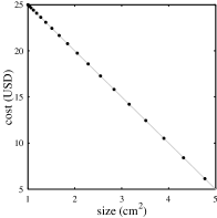
(a) non-uniform—biased to one end

(b) non-uniform—biased to both ends

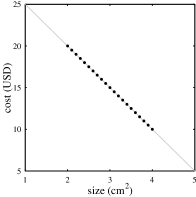
(c) uniform—concentrated in the middle

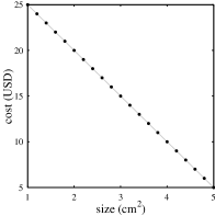
(d) uniform and cover the entire PF

Figure 2.7: Different distributions of solutions across the PF

Chapter 3 Evolutionary Algorithms

3.1 Introduction

During The Voyage of the Beagle (1831–1836), Charles Darwin (1809–1882) noticed that most species produce more offspring than can grow to adulthood, however the population size of these species remains roughly stable. It was the struggle for survival that stabilizes the population size given the limited, however, stable food resources. He noticed also that among sexually reproductive species no two individuals are identical, although many of the characteristics they bear are inherited. It were the variations among different individuals that directly or indirectly distinguished them among other species and their peers, and rendered some of them more suitable to their environment that the others. Those who are more fit to their environment are more likely to survive and reproduce than those who are less fit to their environment. Which means that the more fit individuals have greater influence on the characteristics of the following generations than the less fit individuals. This process results in offspring that evolve and adapt to their environment over time, which ultimately leads to new species [35]. Darwin has documented his observations and hypotheses in his renowned yet controversial book “On the Origin of Species” [35] which constituted the Darwinian Principles.

Although Darwinian principles brought a lot of contention due to apparent conflict with some religious teachings to the point that some clergymen considered it blasphemy, these principles captured the interest of many naturists and scientists. It wasn’t until the 1950’s when computational power emerged and allowed researchers and scientists to build serious simulation models based on Darwinian principles [36]. During the 1960’s and 1970’s, the field of Evolutionary Computation (EC) started to take ground by the work of Ingo Rechenberg [37], John Bagley [38], John Holland [39] and Kenneth De Jong [40]. Those researchers developed their algorithms and worked separately for almost 15 years until early 1990’s when the term CI and its subfields were formalized by the IEEE Neural Network Council and the IEEE World Congress on Computational Intelligence in Orlando, Florida in the summer of 1994 [41]. Since then, these various algorithms are perceived as different representations of a single idea. Currently, EC along with SI, Artificial Neural Network (ANN), Fuzzy systems among other emerging intelligent agents and technologies are considered subfields of CI [42].

Researchers have utilized different EC models in analyzing, designing and developing intelligent systems to solve and model problems in various fields ranging from engineering [41, 43], industrial [44], medical [45, 46], economic [47] among many others [48]. For a comprehensive record on EC history the reader may refer to [49, 48, 50]

3.2 How and Why They Work?

EAs are a subfield of EC. They are biologically- and nature-inspired algorithms. They work by evolving population of potential solutions to a problem, analogous to populations of living organism. In real-world, individuals of a population vary in their fitness to their environment, some of them can defend themselves against attacks, while others can’t survive an attack and perish. Some can provide food for themselves and their offspring all the time, while others may not survive a short famine and starve to death. In EAs, individuals of a population, likewise, are not equally fit. Due to differences in their characteristics some of them are more fit than the others, and because the resources that keep them alive are limited, the more fit is the individual the more likely it will survive and take part in new generations. Those who are fit enough to survive have the chance to mate with other fit individuals and produce offspring that carry a slightly modified version of their parents’ good characteristics. But those fertile parents produce more offspring than their environment resources can support. So the best of the good individuals in the population will survive to the next generation and start a new cycle of mating, reproducing and fighting for survival. This cycle is shown in Figure 3.1, where terminate is the termination condition; it could be a certain number of generations or an error tolerance value or any other condition. As generations pass by, the average fitness of individuals increases because they adapt to their environment. Which means that this population of evolving solutions will explore the solution space looking for the best value(s) and will progressively approach it(them).

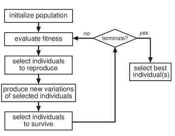
Figure 3.1: Evolutionary Algorithms procedure

The idea of using Darwinian selection to evolve a population of potential solutions has a another great benefit in solving dynamic problems. Because most real-life problems are dynamic, the definition of fitness and the rules of the problem may change once the problem has been formalized. So it will be useless to solve the problem using the old rules because it means solving a problem that does not exist any more. However, by using a population of evolving solutions, individuals adapt to the new rules of their environment over time.

EAs are a collection of algorithms that share the theme of evolution. The mainstream instances of EAs comprise Genetic Algorithms (GAs) [39], Evolutionary Strategies (ES) [37], Evolutionary Programming (EP) [51]. In addition to those three methods, Genetic Programming (GP) [52, 53], Learning Classifier Systems (LCS) [54, 55] and hybridizations of Evolutionary Algorithms with other techniques are classified under the umbrella of EAs as well [56].

3.3 Genetic Algorithms

Genetic Algorithms are the most popular method among all EAs. It was proposed by John Holland in 1962 [57] during the wake of the quest for the general problem solver [58, 59, 60]. GA is a biologically-inspired algorithm. It evolves a population of individuals encoded in bitstrings (some variations of GA use real numbers representations). By analogy to biology, the encoded bitstring structure of an individual in a population is known as a chromosome. Figure 3.2 shows an example of chromosomes consisting of 8 bits each.

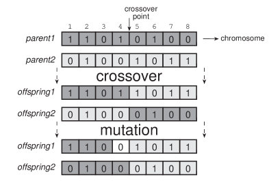
Figure 3.2: Genetic variations

A GA solver starts its procedure by creating a population of individuals representing solutions to the problem. The population size (the number of individuals in the population) is among the parameters of the algorithm itself. A big population size helps exploring the solution space but is more computationally expensive than a smaller population which may not have the exploration power of the bigger population. After the population is created, the fitness of its individuals is evaluated using the fitness function. The fitness function is a property of the problem being optimized and not the algorithm. It reflects how good is a potential solution and how close it is to the global optimum or the PF. So, a good knowledge of the problem is required to create a good fitness function that describes the problem being optimized as accurately as possible. After evaluating their fitness, some individuals are chosen to reproduce and are copied to the mating pool. The number of individuals to be chosen (the size of the mating pool) is a parameter of the algorithm. Different mechanisms of selecting which individuals to reproduce is explained in Subsection 3.3.2, but for now it is enough to say that most of these mechanisms favor individuals with higher fitness values over those with lower fitness values. The next step is to match those individuals for reproduction which is done by random in most cases.

Two variation operators are applied on the matched individuals (parents) to produce their offspring. The fist variation operator is the crossover between the parents’ chromosomes. As shown in Figure 3.2, parent1 and parent2 are two matched individuals. The chromosomes of those two parents are cut at the crossover point (between bit #4 and bit #5), and the resulting half chromosomes are swapped to create two offspring, offspring1 and offspring2. It is to be noted however that the crossover operator may not be applied on all parents in the mating pool. The crossover ratio defines the percentage of parents in the mating pool which will be affected by the crossover operator. This value is algorithm dependent but it varies around 0.9 for most GA implementations [61]. After the crossover is done, the offspring chromosomes are mutated. Mutation of chromosomes in binary representation is done by flipping one or more bits in a chromosome. As shown in Figure 3.2, offspring1 was mutated by flipping its $4^{\text{th}}$ bit from $1\to 0$. As the case with the crossover operator, the mutation operator may not affect all individuals. The ratio of mutated bits to the total number of bits is known as the mutation ratio and is typically below one percent [61]. As the mutation ratio increases, the algorithm becomes more a random search algorithm.

The offspring join the population after evaluating their fitness to fight for survival. This stage is crucial for all individuals; based on their fitness, some of them will survive to the next generation, while others will perish. Different mechanisms can be used to select surviving individuals. Many of which are probabilistic techniques that favor more fit individuals.

The surviving individuals make-up a new generation and restart the cycle of fitness evaluation, mating selection, reproduction and survival selection. This cycle is repeated until a stopping condition is met, which could be the number of cycles, the solution error of the best individual or any other condition or mix of conditions set by the algorithm designer.

GAs are flexible problem solvers; they are less dependent on the problem being solved than traditional techniques. Moreover they provide high degree of flexibility for their designer. A GA designer can choose a suitable representation scheme, a mating selection technique and the variation operators of his choice.

3.3.1 Representations

How can a GA be less dependent on the problem being optimized than a traditional technique? The answer is because the problem is being transformed to the algorithm domain before the GA starts solving the problem. Some people even argue that a GA is problem independent because this transformation is done before the algorithm is invoked. The transformation to the problem domain is done mainly by providing an encoding mechanism for possible solutions to the problem, aka ’representation’, and by creating a fitness function.

The choice of which representation to use should be done within the context of the problem. A good representation for a scheduling problem may not be suitable for the Rastrigin problem given earlier in Section 2.1 and vice versa.

Binary Representations

The oldest and most used scheme of representation is the binary representation. As shown in Figure 3.3, a chromosome consists of a string of bits, each one of those bits is known as an allele. A gene is a combination of one or more alleles which determine a characteristic of the individual. For example, if the chromosome shown in Figure 3.3 is for an imaginary creature, then the three circled alleles $[0~{}1~{}0]$ may represent its eye color gene, and by varying the values of those three alleles its eye color will change.

Figure 3.3: Chromosome structure

To use binary representation for a combinatorial problem, each possible solution to the problem can be represented by a unique sequence of digits. For example, the solutions of the SAT problem given in Subsection 2.3.1 can be directly transformed to bitstrings. So the chromosome $[0111001101]$ will be one of $2^{10}$ different solutions to the 10-variables SAT problem.

However, using binary representation to encode real valued solutions of the Rastrigin problem will work differently. First, the search space or the solution space is continuous, which means there are infinite number of possible solutions, so it must be sampled. A very small sampling step leads to huge number of possible solutions which fairly represents the solution space but it will be computationally expensive to search this huge number of solutions. While a big sampling step make it less expensive but on the expense of a bad representation of the solution space. If the precision used to sample the Rastrigin problem is four digits after the decimal point it means that there are $6-(-6)\times 10000=120000$ possible solutions, which requires 17 digits to represent them. So, $-6\to 00000000000000000$ and $6\to 11111111111111111$. A transformation of the binary string $<b_{0}b_{1}\dotsm b_{17}>$ back to the decimal form is done by transforming the binary number to a decimal one $x^{\prime}$ then using the following rule:

$$x=-6+\frac{12x^{\prime}}{2^{17}-1}$$ (3.1)

So the solution $01001011101101111$ is transformed to the decimal number $x^{\prime}=38767$ then by using (3.1)

$$x=-6+\frac{12\times 38767}{2^{17}-1}=-2.4507$$ (3.2)

Real-valued Representations

It could be more suitable for problems with real valued solutions to be represented using a real-valued representation. In this representation, each individual is a real valued number that expresses the value of the solution. Using this representation, there is no need to define a solution precision, such as the one defined for the binary representation, because the search or variation operators will be able to transform this solution to any of the infinite number of possible solutions in the solution space (if the floating point precision of the computer used to solve the problem is unlimited). However this type of representation requires another mechanism of crossover and mutation as explained in Subsection 3.3.3.

Integer Representations

For permutation problems, it might be more intuitive to represent solutions using integer values. This is illustrated using the following Traveling Salesman Problem (TSP) example.

The TSP is a combinatorial optimization problem that has been extensively studied in the last 150 years [62] due to its numerous applications such as in transportation, networking and printed circuit manufacturing. The problem is defined as [62]: given $n$ cities and their intermediate distances, find a shortest route traversing each city exactly once.

As shown in Figure 3.5, a possible route the traveling salesman can take is $1\to 5\to 3\to 2\to 4\to 1$. This route can be directly mapped to and represented by the string of real numbers $[1~{}5~{}3~{}2~{}4~{}1]$, where the integers represent the cities to be visited by the order they are stored in the string.

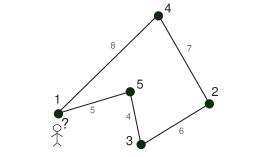
Figure 3.4: The traveling-salesman problem

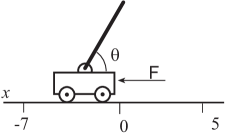
Figure 3.5: The inverted pendulum problem

Problem-Specific Representations

Using only one of the previously mentioned representations to represent all the variables of a problem may not be the best option for some problems, which is the case in the following example; The inverted pendulum problem shown in Figure 3.5 is a classic problem in control engineering. The objective is to construct a function that maps the system states to a horizontal force applied on the cart carrying the inverted pendulum to stabilize it vertically. The states of this problem are the position of the cart $x$, its speed $\dot{x}$, the angular position of the pendulum $\theta$ and its angular velocity $\dot{\theta}$. For such a problem the parameters $x,\dot{x},\theta,\dot{\theta}$ will be the input to the function and the output will be the applied horizontal force. This problem can be represented using a parse tree of symbolic expressions [52, 63, 15]. The parse tree consists of operators, such as ($+,~{}-,~{}\cos,~{}\sin,~{}\times,~{}\exp,\dotsm$) and arguments, such as ($x,~{}\theta,~{}t,~{}r,\dotsm$). A possible tree may look like:

$$(\times(\cos(+(x)(3.14)(\theta)))(t))$$ (3.3)

which is equivalent to:

$$t\cos(x+\theta+3.14)$$ (3.4)

More on Representations

The three schemes of representations mentioned above are by no means exhaustive. An algorithm designer may come up with his own representation which may better suit his problem. However, the representation scheme, as mentioned before, should never be considered independent of the problem; If the variation operators used do not suit the representation, they may produce offspring who are totally different from their parents, which acts against the learning process because the algorithm samples new trials from the state space of possible solutions without regard for previous samples. This procedure may perform worse than random search [15]

Some representations incorporate the constraints of the problem and provide feasible solutions for the problem all the way. Although it may be desirable to evolve feasible solutions all the time and not to worry about the constraints or define them explicitly in the problem, it is useful to allow the algorithm to evolve few infeasible solutions to explore the solution space for possible scattered feasible regions that may contain better values.

3.3.2 Mating Selection

After a decision about how solutions will be represented is made, the next step is to decide about the mating selection procedure. Mating selection focusses on the exploration of promising regions in the search space [64]. It tends to select good individuals to mate—hoping that their offspring will be as good or better than them because they will inherit many of their parents’ characteristics. However, if the selection procedure strictly selects the very few top of the population, the population will lose its diversity because after few generations the population will only contain a slightly different copies of few individuals who were the best in their generations, and if this procedure continues, the population will be made-up of almost identical individuals after few more generations. The main idea behind a GA is to evolve a population of competing individuals, so if the individuals became identical, there will be no competition and henceforth no evolution. So, keeping a diverse population indeed helps the algorithm explore the search space [63]. The degree to which the algorithm favors and selects the best individuals in the population for mating is measured by the selection pressure. The selection pressure is defined as “the ratio of the probability of selecting the best individual in the population to that of an average individual” [64]. As the selection pressure increases, the algorithms tends to choose the very best of the population to mate and produce the next generation leading to a population that converges to a local optima, this situation is known as premature convergence. On the other hand, if the selection pressure decreases, the algorithm will converge slowly and wander in the search space. It should be clear that the selection pressure is not a parameter that the algorithm designer explicitly set its value, instead, it is influenced by different aspects of the algorithm, especially the selection mechanism used. It is to be noted that the following selection mechanisms define the preference of selecting an individual in the population, however the number of offspring this individual produces for each mating process is another issue.

Fitness Proportionate Selection

Fitness Proportionate Selection (FPS) is one of the earliest selection mechanisms proposed by Holland [39] (Sometimes known as roulette wheel selection). It selects individuals based on their absolute fitness. That is, if the fitness of an individual $j$ in the population is $f_{j}$, the probability of selecting this individual is $z_{j}=\frac{f_{j}}{\sum_{i=1}^{N}f_{i}}$, where $N$ is the population size. This selection mechanisms allows the most fit individuals in population to multiply very quickly early in the run and take over the population, and after few more generations the diversity almost vanishes and the selection pressure becomes very low leading to stagnant population. In other words, leading to premature convergence. Another handicap of this mechanism is that it behaves differently on transposed versions of the same fitness function [65]. For example, given a population of two individuals $a$ and $b$ with fitness values 1 and 2, respectively. The probability of choosing the first individual is $\frac{1}{3}=0.33$ while that of the second is $\frac{2}{3}=0.67$, this is a $1:2$ ratio. However if a constant value of 10 is added to the fitness values of the population the probabilities will become $\frac{11}{23}=0.48$ and $\frac{12}{23}=0.52$ which is almost a $1:1$ ratio.

A possible remedy to the weak selection pressure and the inconsistent behavior of the algorithm along the run can be achieved by subtracting the fitness of the worst individual in the population of a window containing the last $n$ generations. This approach can be considered as a dynamic scaling of the population fitness.

Another possible solutions is achieved by using Goldberg’s sigma scaling method [54], which scales the fitness of individuals using the mean $\bar{f}$ and standard deviation $\sigma_{f}$ of fitness in the population.

$$f^{\prime}(x)=\min(f(x)-(\bar{f}-c\cdot\sigma_{f}),0)$$ (3.5)

Rank Selection

Another way to overcome the deficiencies of the FPS is to use the rank selection. As its name implies, this procedure orders all individuals in the population according to their fitness, and then selects individuals based on their rank rather than their absolute fitness such as in FPS. This methods maintains a constant selection pressure because no matter how big is the gap between the most and least fit individuals in a population, the probability of selecting each one of them will remain the same as long as the population size remains the fixed.

After the individuals are ordered in the population, they are assigned another fitness value inversely related to their rank. The two most used fitness assignment functions result in linear ranking and exponential ranking.

For linear ranking, the best individual is assigned a fitness of $s\in[1,2]$, while the worst one is assigned a value of $2-s$. The fitness values of the intermediate individuals are determined by interpolation. This can be achieved using the following function:

$$f(i)=s-\frac{2(i-1)(s-1)}{N-1}$$ (3.6)

Where $i$ is the individual rank $i\in[1,N]$ and $N$ is the number of individuals. For linear ranking, the selection pressure is proportional to $s-1$.

For nonlinear ranking, the best individual is assigned a fitness value of 1, the second is assigned $s$, typically around 0.99 [66], the third $s^{2}$, and so on to lowest ranked individual. The selection pressure for nonlinear ranking is proportional to $1-s$.

Tournament Selection

Unlike previously mentioned selection procedures, the tournament selection does not require a knowledge about the fitness of the entire population, which can be time consuming in some application with huge populations which requires fast execution. It is suitable for for some situations with no universal fitness definition such as in comparing two game playing strategies; it might be hard to set a fitness function that evaluates the absolute fitness of each of those two strategies, but it is possible to simulate a game played by those two strategies as opponents, and the winner is considered the fittest.

Tournament selection picks $k$ individuals by random from the population and selects the best one of them for mating. This does not require a full ordering of the sample nor an absolute knowledge of their fitness. The selection pressure of this mechanism can be varied by changing the sample size $k$, it increases by increasing $k$ and reaches the maximum at $k=N$. This selection mechanism can be used with or without replacement. Moreover a non-deterministic selection can be used, which means that the probability of selecting the best individual in the sample is less than one to give a chance for the worst individual in the population to be selected, otherwise, it will never be selected.

This selection mechanism is the most widely used because it is simple, does not require knowledge of the global fitness, adds low computation overhead and its selection pressure can be easily changed by varying the sample size $k$. A common sample size is $k=2$ [67].

For more mating selection techniques the reader may refer to [66, 68].

3.3.3 Variation Operators

In real-world, although parents and their offspring have common characteristics, they are never identical; Like father like son, but the son is not a clone of the father. This variation among individual was noted by Charles Darwin in his controversial book [35] where he emphasized that this variation is a major force that drives the evolution process. To mimic this process in GAs, researchers have developed variation operators that help the algorithm search the solution space, henceforth, they are sometimes known as search operators. These variation operators have two goals: The first one is to produce offspring that resemble their parents, while the second one is to slightly perturb their characteristics. The oldest and most widely used variation operators are the crossover and the mutation operators [39]. They were proposed by John Holland to operate on binary GAs, however many other variation operators were proposed to operate on other forms of GA representations [69]. It is to be noted that all syntactic manipulations by variation operators must yield semantically valid results [70].

Crossover

The fact that the offspring very often look much like their parents intrigued Gregor Mendel (1822–1884) and lead him to do his famous experiments on pea plants. By analyzing the outcomes of his experiments on some 28000 samples he reached a conclusion about the rules of inheritance and published these findings in a paper [71] which is considered to be the basis of modern day genetics rules. Researchers in GAs were inspired by these rules and used a modified version of them in their algorithms [39], and from there came the GA crossover operator.

A recombination operator is known to be an exploitation operator because it exploits the accumulated knowledge in the current solution vectors by using parts of them as building blocks of their offspring. It is widely believed among AI community that exploitation should be emphasized at later stages of the search to prevent premature convergence [72, 73].

Different versions of the crossover operator are applied to binary, real-valued, and parse tree representations but they essentially do the same job; They simply create the genes of an offspring by copying a combination of its parents genes.

n-point crossover [40] is used mainly for binary representations. The operator randomly picks $n$ points along a copy of the two parents chromosomes, divide each one of them into $n+1$ parts, and then swap some of these parts to create the offspring chromosomes. Figure 3.6 shows an example of a 3-point crossover operation. First, the crossover points are randomly assigned the positions shown in figure, dividing each parent into 4 parts. Then, offspring1 is created by copying the first and third parts of parent1, and the second and fourth parts of parent2. While offspring2 is created by copying the first and third parts of parent2, and the second and fourth parts of parent1. The probability of independently crossing over each individual in the mating pool is known as the crossover ratio $p_{c}$.

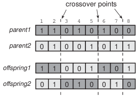
Figure 3.6: Crossover in binary GA

Uniform crossover is another alternative to use with binary GAs. The number of crossover points in this operator is not fixed, instead, it creates each allele of the offspring by copying one of the two corresponding alleles in its parents with a certain probability. This procedure can be explained using the following Matlab code:

Uniform crossover procedure (Matlab code)

⬇

z = 0.5; % z is the crossover probability

o = p1; % o is an offspring, p1 is the first parent

for i = 1 : k % k = chromosome length

x = rand; % random number in the range (0, 1)

if (x>z)

o(i)=p2(i); % copy the i allele of parent2 to offspring

end

end

By increasing the value of $z$, the offspring alleles will be more like those of p1. The previous code is repeated for each offspring.

A real-valued representation can be transformed into binary representation to apply a binary crossover operator as shown previously, and then get transformed back to real-valued representation, but it is not recommended to follow this procedure and add such a computational cost and sacrifice precision due to sampling and rounding-off errors encountered in decimal–binary—binary–decimal conversion. Instead, it is recommended to apply some of the recombination operators specially made for real-valued representations.

The blending methods create the variables of the offspring by weighting the corresponding variables in their parents chromosomes. For example, to create the variables in the offspring chromosome, the following rule can be used:

$$o_{1,i}=\beta p_{1,i}+(1-\beta)p_{2,i}$$ (3.7)

$$o_{2,i}=(1-\beta)p_{1,i}+\beta p_{2,i}$$ (3.8)

Where $o_{1,i}$ is the $i^{\text{th}}$ variable of the first offspring, and $\beta$ is the weighting factor in the range [0,1]. The higher the value of $\beta$, the more the offspring will look like the first parent ($p_{1}$), and the lower $\beta$ gets, the more the offspring will resemble the second parent ($p_{2}$).

The Simulated Binary Crossover (SBX) operator is a recombination alternative to consider for real-valued representations. This operator was proposed by Deb [69], and he claims that it provides self-adaptive search mechanism [74]. This operator is explained using the following rules:

$$o_{1,i}=0.5[(1+{\beta}_{i})p_{1,i}+(1-{\beta}_{i})p_{2,i}]$$ (3.9)

$$o_{2,i}=0.5[(1-{\beta}_{i})p_{1,i}+(1+{\beta}_{i})p_{2,i}]$$ (3.10)

and ${\beta}$ is evaluated using the following rule:

$$\beta=\left\{\begin{aligned} &(2u)^{\frac{1}{\eta+1}},&\quad&\text{if}\quad u\leq 0.5\\ &\left(\frac{1}{2(1-u)}\right)^{\frac{1}{\eta+1}},&&\text{otherwise}\end{aligned}\right.$$ (3.11)

where $u$ is a uniformly distributed random number in the range $(0,1)$, and $\eta$ is a distribution index; a low value of $\eta$ (less than 2) gives high probability of producing offspring different from their parents, while a high $\eta$ value (greater than 5) means that the offspring will be very close to their parents in the solution space.

For parse tree representations, a recombination operator do swap subtrees of the solution vectors. For example, given the following solution vector

$$(+(\cos(\exp(3)(7)))(\times(4)(\log(3))))$$ (3.12)

by swapping the subtrees $\exp(3)(7)$ and $\times(4)(\log(3))$, it becomes

$$(+(\cos(\times(4)(\log(3))))(\exp(3)(7)))$$ (3.13)

However care must be taken to prevent trees from growing rapidly and reaching an extremely long length, because it may halt the machines executing the algorithm. This is known as bloating, and it is a major concern in GP implementations.

Mutation

Unlike recombination operators, mutation operators do not make use of the knowledge of the search space acquired through generations, they do perturb the population by providing random genetic material provided they result in semantically valid results.

For binary GAs, the mutation operator first determines the positions of the alleles that will undergo mutation. However, the choice of these alleles is made at random with equal probability for each one of them to be mutated (uniform distribution), and their number is determined using the mutation ratio $p_{m}$, which is the probability of independently inverting one allele. Second, the operator flips the selected alleles to produce the mutated offspring. For example, given a pool with two solution vectors $a_{1}=1001101011$, $a_{2}=1011011110$, and $p_{m}=0.1$. A mutation operator being applied on them will mutate $0.1\times 2\times 10=2$ alleles, and may turn the solution vectors into $a_{3}=10\boldsymbol{1}11010\boldsymbol{0}1$, $a_{4}=1011011110$, respectively. Note that the two alleles to be mutated happened to be at the first solution vector (shown in boldface), while the second one remained intact.

Mutating real-valued GA pose some challenges. If the mutation operator does not operator on specific values of the parents [75], it will allow the offspring escape local optima and will help the algorithm explore new regions of the search space. But it will break the link between the parents and their offspring instead of causing causing small perturbation. On the other hand, if the mutation operator do operate on specific values of the parents to produce their offspring, it may not be very helpful in escaping local optima, but will keep the link between the parents and their offspring. The later approach will be further explained here.

For a $n$-dimension solution vector $\text{\bf x}\in\mathbb{R}^{n}$ the mutation operator will be in the form [76]

$$\text{\bf x}^{\prime}=m(\text{\bf x})$$ (3.14)

where x is the parent solution vector, $m$ is the mutation operator, and $\text{\bf x}^{\prime}$ is the mutated offspring solution vector. The mutation operator $m$ may simply add a real random variable M to the parent vector

$$x_{i}^{\prime}=x_{i}+M_{i}$$ (3.15)

where $x_{i}$ is the $i^{\text{th}}$ variable of the solution vector x. It is recommended to create M with a mean value of 0 to prevent a bias towards some parts of the search space and keep the offspring uniformly distributed around their parents. If M has a uniform distribution in the range $[-a,a]^{n}$, it will be equally probably that $\text{\bf x}^{\prime}$ will take any value in the hyper-box $[\text{\bf x}-a,\text{\bf x}+a]^{n}$ if mutated. Alternatively, M can have a normal (or Gaussian) distribution which can be represented by the following equation:

$$M_{i}=\frac{1}{\sigma\sqrt{2\pi}}\,\exp\left(-\frac{(x_{i}-\mu)^{2}}{2\sigma^{2}}\right)$$ (3.16)

where $\sigma$ is the standard deviation, and $\mu$ is the mean. If $\mu$ is set to 0, the value of $\sigma$ will determine the probability of different mutation strengths; As $\sigma$ increases, it becomes more probable that the offspring will lie away from its parent, while decreasing $\sigma$ value increases the probability of producing offspring that looks similar to its parent.

The Polynomial Mutation is another mutation operator for real-valued GAs [69, 77]. The offspring is mutated using the following rule

$$x_{i}^{\prime}=x_{i}+(x_{iu}-x_{il})\delta_{i}$$ (3.17)

where $x_{iu}$ and $x_{il}$ are the upper and lower bounds of the variable $x_{i}$, respectively, and $\delta_{i}$ is calculated from a polynomial distribution by using

$$\delta_{i}=\left\{\begin{aligned} &(2r_{i})^{\frac{1}{\eta_{m}+1}}-1\qquad&\text{if}\;r_{i}<0.5\\ &1-[2(1-r_{i})]^{\frac{1}{\eta_{m}+1}}\qquad&\text{otherwise}\end{aligned}\right.$$ (3.18)

where $r_{i}$ is a uniformly distributed random number in the range $(0,1)$, and $\eta_{m}$ is a mutation distribution index.

The final mutation operators to be presented here is the parse tree mutation operators. Among many operators, Angeline defines four mutation operators [76]. The grow operator randomly selects a leaf from the tree and replace it with a randomly generated subtree (Figure 3.7a). The shrink operator randomly selects an internal node from the tree and replaces the subtree below it with a randomly generated leaf (Figure 3.7b). The switch operator randomly selects an internal node from the tree and rearrange its subtrees (Figure 3.7c). While the cycle operator randomly selects a node from the tree and replaces it with another node, provided that the resulting tree is a valid one (Figure 3.7d).

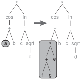
(a) grow

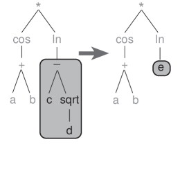
(b) shrink

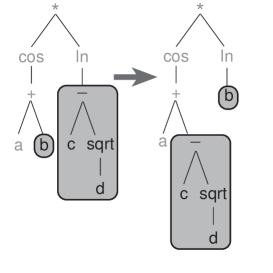
(c) switch

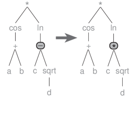
(d) cycle

Figure 3.7: Mutation methods for a parse tree

3.3.4 Schema Theorem

In his early work on GAs, John Holland presented the schema as a building block for individuals in a population. While explicitly evaluating the fitness of the individuals, a GA implicitly evaluates the fitness of many building blocks without any added computation overhead (implicit parallelism). As the search for the optimal solution progresses, the algorithm focusses on promising regions of the search space defined by schemata having fitness above the average of the population in their generations (above-average schemata); The more fit are the individuals a schema produces, the more samples will be produced from this schema [63]. The following discussion on schemata assume a binary GA representations.

A schema is a template for solution vectors. It defines fixed values for some positions, and assumes don’t care values for the other positions. For example, given the following solution vector $S_{1}$ of length $m=10$

$$S_{1}=(*~{}1~{}1~{}1~{}0~{}*~{}*~{}0~{}1~{}*)$$ (3.19)

there are six fixed positions (taking a value of ‘1’ or ‘0’), and four don’t care positions (marked by ‘*’). The number of the fixed positions in a schema is known as the order or the schema. So the order of the $S_{1}$ schema is $o(S_{1})=6$. Another property of the schema is its defining length, which is the distance between the first and last fixed positions in a schema. The defining length of the $S_{1}$ schema is $\delta(S_{1})=9-2=7$

Any schema may produce $2^{d}$ distinct individual, where $d$ is the number of don’t care positions in this schema. On the other hand, any solution vector can be matched by $2^{n}$ different schemata. It is clear that the schema $(*~{}*~{}*~{}*~{}*~{}*~{}*~{}*~{}*~{}*)$ is the most general schema; It matches $2^{10}$ solution vector (which includes the entire population). While $(1~{}1~{}1~{}1~{}1~{}1~{}1~{}1~{}1~{}1)$ is among the most specific schemata; It matches a single solution vector, namely $(1111111111)$.

Another property of a schema is its fitness at time $t$, $f(S,t)$. The fitness of a schema is defined as the average fitness of all individuals in the population matched by this schema [78].

Given a population of size $N$, with solution vectors $\text{\bf x}_{i}$ of length $m$ and a fitness function $f$. The schema $S$ which matches $w$ individuals $(\text{\bf x}_{1},\dotsm,\text{\bf x}_{w})$ in the population at time $t$ will have an average fitness of

$$f(S,t)=\frac{1}{N}\,\sum_{i=1}^{w}f(\text{\bf x}_{i})$$ (3.20)

If the number of individuals matched by schema $S$ is $\xi(S,t)$ and their average fitness is $\frac{f(S,t)}{F(t)}$, where $F(t)=\sum_{i}^{N}f(\text{\bf x}_{i}(t))$, then it is expected that for the next generation the number of individuals matched by $S$ will be

$$\xi(S,t+1)=\frac{\xi(S,t)\times N\times f(S,t)}{F(t)}$$ (3.21)

if the average fitness of the population is $\overline{F}(t)=\frac{F(t)}{N}$, the the previous equation can be rewritten as

$$\xi(S,t+1)=\frac{\xi(S,t)f(S,t)}{\overline{F}(t)}$$ (3.22)

From the last equation, it is clear that if the schema is above-average for the current generation ($f(S,t)>\overline{F}(t)$), then the number of individuals matched by this schema will increase in the next generation. But if the schema is below-average, the number of individuals this schema matches will decrease in the next generation.

If $\xi(S,0)$ is known, then $\xi(S,t)$ can be directly evaluated from (3.22)

$$\xi(S,t)=\xi(S,0)\,\left(\frac{f(S,t)}{\overline{F}(t)}\right)^{t}$$ (3.23)

assuming that $S$ will maintain a fixed above-average fitness through generations.

The reproductive schema growth equation (3.23) only considers selection and ignores the effect of crossover over the population. To understand how crossover may disrupt a schema, the following example is presented

If the two solution vectors $\text{\bf x}_{1}=(0111010010)$, which is counted among $\xi(S_{1},t)$, and $\text{\bf x}_{2}=(0110100101)$ do exist in a population, and the crossover operator decided that those vectors will be crossed-over right after the sixth allele. none of the two offspring solution vectors produced ($\text{\bf o}_{1}=(0111010101)$, and $\text{\bf o}_{2}=(0110100010)$) will be matched by the schema $S_{1}$. However, if the crossover operation took place right after the third allele, the offspring will look like $\text{\bf o}_{1}=(0110100101)$, and $\text{\bf o}_{2}=(0111010010)$, and there will be one solution vector ($\text{\bf o}_{2}$) matched by $S_{1}$. Which means that equation (3.23) is not accurate.

It is clear that a higher defining length for a schema increase the probability of its destruction, because it will be more likely that the crossover point will fall between the first and the last fixed positions of the schema. Henceforth, given the crossover rate ($p_{c}$), the probability of schema survival will be $1-p_{c}\frac{\delta(S)}{m-1}$. But the crossover operation may not destroy the schema even if it splits the vectors between two fixed positions; It is possible to crossover two solution vectors matched by the same schema, so regardless of the crossover position, the two resulting offspring would still be matched by that schema. So, the probability of schema survival will slightly increase, and the reproduction schema growth equation will look like;

$$\xi(S,t+1)\geq\left(\frac{\xi(S,t)f(S,t)}{\overline{F}(t)}\right)\left(1-p_{c}\,\frac{\delta(S)}{m-1}\right)$$ (3.24)

To make the above equation more accurate, the mutation operator should be considered as well.

The mutation operator will destroy a schema only if it inverts one of its fixed positions. So, the higher the order of a schema is, the more likely it will be destroyed by a mutation operator. Henceforth, given the schema order ($o(S)$) and the mutation ratio ($p_{m}$). The probability that a fixed position will survive mutation is ($1-p_{m}$), and the probability of schema survival is $(1-p_{m})^{o(S)}$, which for normal mutation ratios ($p_{m}\ll 1$) can be approximated to $(1-o(S)\times p_{m})$. The reproduction schema growth equation will now look like:

$$\xi(S,t+1)\geq\left(\frac{\xi(S,t)f(S,t)}{\overline{F}(t)}\right)\left(1-p_{c}\,\frac{\delta(S)}{m-1}-o(S)p_{m}\right)$$ (3.25)

This equation shows how fast a schema may influence the population; The number of individuals created using this template exponentially increases over time if this schema is above-average and has sufficiently short defining length and low order. This equation shows also that a schema with relatively short defining length and low order will be sampled more than another schema with longer defining length and higher order.

Theorem 1 (Schema Theorem).

Short, low-order, above-average schemata receive exponentially increasing rate of trials in subsequent generations of a genetic algorithm.

For a better understanding of the schema theorem and theoretical data given above ,the following example is given.

A GA is running a population of size $N=500$, with individuals of length $m=20$. It has a crossover and mutation ratios of $p_{c}=0.7$ and $p_{m}=0.01$ respectively. When the optimizer was initialized there was 5 individuals matched by the schema $S_{a}$ after initialization, $\xi(S_{a},0)=5$.

Using the reproduction schema growth equation, given in (3.25), two tables are created; Table 3.1 illustrates the effect of the schema/population fitness ratio on the schema growth rate, while $\delta(S_{a})=11$ and $o(S_{a})=6$, and Table 3.2 shows the effect of different defining length and order values for schema $S_{a}$ on its growth rate, while $\frac{f(S,t)}{\overline{F}(t)}=1.9$.

The values shown in the body of the two tables are the expected number of individuals that schema $S_{a}$ will match through generations (rounded to floor), and a “–” entry means that the overwhelming number of schema instances in the population caused violation of the assumed average population fitness.

Table 3.1: Effect of schema/population fitness ratio on schema growth rate

	Generations
$f(S)/\overline{F}$	1	10	20	30	40	50	60	70	80	90	100
1.8	5	4	2	2	1	1	1	0	0	0	0
1.9	5	6	7	8	9	11	13	15	18	21	24
2.0	5	9	18	35	69	134	263	–	–	–	–
2.1	5	14	45	144	–	–	–	–	–	–	–
2.2	5	22	110	–	–	–	–	–	–	–	–

Table 3.2: Effect of schema defining length and order on schema growth rate

	Generations
$(\delta~{},~{}o)$	1	10	20	30	40	50	60	70	80	90	100
(10, 6)	5	11	24	55	125	285	–	–	–	–	–
(10, 7)	5	9	17	33	63	120	229	–	–	–	–
(10, 8)	5	8	12	19	31	50	79	127	203	–	–
(11, 8)	5	4	3	3	2	2	1	1	1	1	1
(12, 8)	5	2	1	0	0	0	0	0	0	0	0

The figures presented in Table 3.1 show how increasing the schema fitness by 10% allows the schema to switch form vanishing (for 1.8 ratio) to exponentially increase its samples (for 1.9 ratio). By increasing the fitness ratio further, the schema takes-over the population more and more faster, until at a fitness ratio of 2.2, $S_{a}$ takes-over the population in less than 30 generations.

Table 3.2 shows how a slight modification of the defining length or the order of the schema can have a significant effect on its growth rate; A unit increase in the defining length (from 10 to 11) leads to $S_{a}$ extinction. A unit increase in the schema order affects its growth rate indeed, but not as dramatically as its defining length.

3.4 Polyploidy

Due to the good results obtained using first GA representations [39, 40], researchers used them without significant modifications. Although, many living organisms carry redundant chromosomes in there cells (polyploid organisms), the effect of polyploidy remains under-researched in Evolutionary Multi-objective Optimization (EMO). In nature, redundant chromosomes help organisms adapt to their environment. When a large asteroid or comet hit earth 65 million years ago, some species adapted to their new environment and survived, dinosaurs failed to adapt and perished. Moreover, these redundant chromosomes help keeping a varied set of organisms to fill different niches in the environment that these organisms live in. A heavy and muscled animal can defend itself against attacks but is slower than a less heavier and less muscled animal which can catch its prey. A trade-off between those two traits (muscles and weight) provides animals with advantages over one another.

Polyploid species have redundant chromosomes in their cells. The alleles which result in an organism that well fits its environment tend more to be expressed (dominant alleles) than the other alleles (recessive alleles). Meanwhile, the other alleles are held in abeyance and rarely expressed until the environment changes to favor one or some them and makes them the new dominant alleles.

Though there are dominance schemes other than simple dominance, such as partial dominance and co-dominance, their effects were not investigated before. This is mainly because most research on polyploidy was carried out on binary problems. In partial dominance, an intermediate value between parents’ alleles is expressed. It provides even more population diversity than simple dominance in which a distinct parent allele is expressed. A classical example of partial dominance is the color of the carnation flower that take variants of the red color due to the presence or absence of the red pigment allele. In the co-dominance scheme, both alleles are expressed. A well known example for co-dominance is the Landsteiner blood types. In this example, both ‘A’ and ‘B’ blood type alleles are expressed leading to an ‘AB’ blood type which carries both phenotypes.

3.4.1 Current Representations

Early work examining the effect of polyploidy in GA goes back to 1967 in Bagley’s dissertation [38] as he examined the effect of diploid representation. In his work he used a variable dominance map encoded in the chromosome. A drawback of his model was the premature convergence of dominance values which led to an arbitrary tie breaking mechanism [79]. This work was followed by a tri-allelic dominance scheme used by Hollstien [80] and Holland [39]. For each allele, they added a dominance value associated and evolved with it. It took values of 0, a recessive 1 or a dominant 1, though they used different symbols.

Unlike previously mentioned work which was done on stationary environments, Goldberg and Smith [79] used a non-stationary environment. They used a 0-1 knapsack problem with two evolving limiting weights. They concluded that the power of polyploidy is in non-stationary problems because of the abeyance of recessive alleles that remember past experiments. However, they did not show the performance of their algorithm in remembering more than two oscillating objectives. This was a big shortcoming, because most real world non-stationary problems are non-cycling problems, they may come out of order, and sometimes never repeat. Ng and Wong [81] argued that the enhanced performance in [79] was due to the slow convergence encountered in the diploid representation. They proposed a dominance scheme that used dominant (0, 1) and recessive (0, 1) alleles and inverted the dominance of alleles whenever the individual’s fitness fall below a 20% threshold value. They reported enhanced performance over tri-allelic representation. Some researchers extended the application of polyploidy beyond GA. Polyploidy was applied to Genetic Programming (GP) as well [82].

All the work previously mentioned were conducted for single objective optimization problems. Most of the researchers used relatively low number of decision variables and binary problems such as the 0-1 knapsack problem. At the same time many of these investigations were concerned with manipulating the simple dominance scheme and comparing its variants. The monoploid number (number of chromosomes in each solution vector) remained constant in most of these investigations. Scarce applications such as [83] were done on Multi-Objective Optimization Problems (MOOP). In [83], diploid vectors were used to search in 2-dimensional space optimizing 3 objectives for a food extrusion process. First, they worked on each objective separately and produced offspring better than the worst individual for this objective (otherwise the offspring is killed) and then Pareto dominance was applied to the combined populations of each objective.

What is common among all previous work is that they used simple dominance where the allele either dominates or recesses, which is not always the case in nature. Partial dominance and co-dominance were not investigated before. Partial dominance produces new phenotypes that help the population to adapt to totally new environments and to remember them. It provides more phenotype diversity than simple dominance. Henceforth, a new model is provided here which differs from other polyploid models [39, 80, 79, 38, 81]. In this model; i) Uniform crossover of each parent chromosomes precedes recombination. ii) The offspring alleles are created from their parents’ alleles using partial dominance. iii) The algorithm is applicable to non-binary problems.

3.4.2 Proposed Representation and Procedure

In biology, ploidy is the number of sets of chromosomes in a cell. A cell that has one set of chromosomes is a monoploid cell, while the one that has two sets is a diploid cell, three sets make it triploid and so on. The term “d-ploid” is used to indicate the ploidy number. So, 1-ploid representation is a monoploid one, 2-ploid representation is a diploid one and so on. In this algorithm the partial dominance scheme is used. The phenotype of each solution vector is based on the partial dominant alleles or the Dominant-alleles-set (DAS) as shown in Figure 3.8. The DAS of any solution vector determines its fitness value. The ploidy number $d$ of a solution vector is the number of all chromosomes in that vector including the DAS chromosome. A detailed procedure of the algorithm is given as follows;

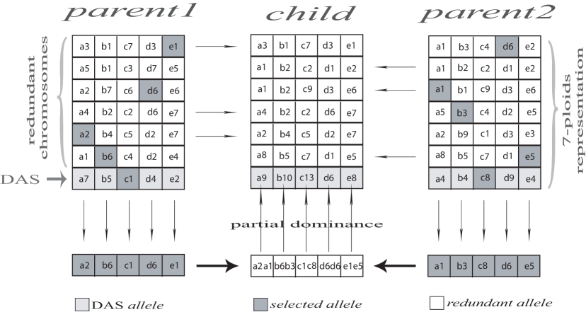
Figure 3.8: The Polyploid mating procedure

1. Initialization: For a $d$-ploid representation. A population of size $N$ is initialized at random by filling each DAS and the $d-1$ chromosomes for each of the $N$ solution vectors. Then, the fitness of each vector is evaluated according to its DAS. The domination of solution vectors is determined based on Pareto dominance.

2. Mating Selection: Only non-dominated solution vectors are selected for mating. This will result in a varying mating pool size and consequently a varying offspring size for each generation, leading to high selection pressure.

3. Variation Operators: After filling the mating pool, two parents are selected at random from the mating pool without replacement. Then, for each parent, an allele representing each locus of a chromosome is randomly selected from all available alleles at this locus to create two sets of alleles (one for each parent). Any recombination operator may be applied to those two sets to create the child’s DAS. Here, the SBX [69] operator is used. Then, the child’s DAS is mutated. Any mutation operator may be used here. Polynomial mutation is used here [69]. After the child’s DAS is created, the remaining $d-1$ chromosomes of this child’s solution vector are selected and copied at random from both parents’ chromosomes. All chromosomes in both parents have the same probability of being selected and copied to carry their genes to later generations. No mutation is applied on these redundant $d-1$ chromosomes.

4. Survival Selection: After evaluating the fitness of the offspring, parents and offspring fight for survival as Pareto dominance is applied to the combined population of parents and offspring. The least dominated $N$ solution vectors (according to number of solutions dominating them) survive to make the population of the next generation. Ties are resolved at random.

Figure 3.8 shows the structure of solution vectors for the Polyploid algorithm. The solution vector parent1 contains the DAS chromosome (the seventh row) plus six more redundant chromosomes (rows 1–6), so this is $6+1=$7-ploids representation. Each one of those seven chromosomes contains five alleles. The DAS chromosome of parent1 vector is [a7 b5 c1 d4 e2], where a7 is the first allele, b5 is the second allele, c1, d4 and e2 are the third, fourth and fifth alleles.

After parent1 and parent2 are selected for mating, for each one of them, an allele is selected to represent each locus (column) of this solution vector as shown in Figure 3.8. For parent1, a2 is selected to represent the first locus (column), b6 to represent the second locus (column), c1, d6 and e1 to represent the third, fourth and fifth loci (columns). Henceforth, paretnt1 is represented by the chromosome [a2 b6 c1 d6 e1]. By following the same procedure, the [a1 b3 c8 d6 e5] chromosome is produced for parent2 . Next, partial dominance is applied on these two chromosomes to get the DAS chromosome of the child solution vector. SBX [69] is used to simulate partial dominance, then polynomial mutation is applied on the produced DAS chromosome. After the child’s DAS chromosome is created and mutated, the remaining 6 chromosomes of the child’s solution vector are filled by copying 6 chromosomes from both parents at random to complete the mating process.

3.4.3 Experiments

In the following experiments the convergence and diversity of solution vectors are measured using two running metrics to understand the behavior of the algorithms. The average orthogonal distance of solution vectors to the PF is used to measure convergence because the equations of the global front are known in advance. While the diversity metric2 presented in [84] is modified and used here to measure diversity of solutions. The modified diversity metric2 is explained as follows:

1. For a given objective, the obtained PF using a population of size $N$ is divided uniformly creating $N$ equal cells on the front surface, such as cells $a$, $b$ and $c$ shown in Figure 3.9. The projection of these cells on the current objective dimension gives $N$ projected cells.

2. The obtained solutions are projected as well on this objective dimension.

3. For every projected cell that contains one or more projected solutions an occupation value of 1 is assigned to it, an occupation value of 0 is assigned to the projected cell otherwise.

4. A diversity value is assigned to each non-boundary projected cell using a sliding window according to the values shown in Table 3.4, where the cell index is $n$. While diversity values for boundary cells are assigned according to Table 3.4, where the boundary cell index is $k$ for the left boundary, and is $k+1$ for the right boundary.

5. The cells’ diversity values are added and divided by the number of cells to give the current objective’s diversity value in the range $(0,1]$.

6. Previous steps are repeated for the remaining objectives.

7. The average diversity value of all objectives is the overall diversity value of the population. The best population distribution yields a diversity value of 1, while this value approaches 0 for the worst distribution.

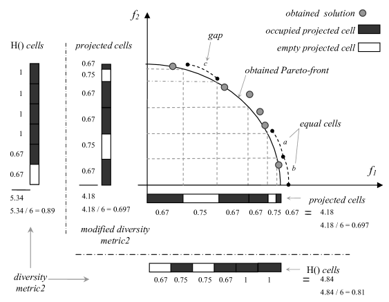
Figure 3.9: Modified diversity metric2 for DTLZ2

Table 3.3: Non-boundary cells’ diversity values

occupation values			diversity
cell($n-1$)	cell($n$)	cell($n+1$)	values
0	0	0	0
0	0	1	0.5
0	1	0	0.75
0	1	1	0.67
1	0	0	0.5
1	0	1	0.75
1	1	0	0.67
1	1	1	1

Table 3.4: Boundary cells’ diversity values        

occupation values		diversity
cell($k$)	cell($k+1$)	values
0	0	0
0	1	0.67
1	0	0.67
1	1	1

Figure 3.9 compares diversity evaluation for the modified and unmodified diversity metric2 for a population of size 6 on a 2-dimensional DTLZ2 [85] minimization problem. To evaluate the diversity value for objective $f_{1}$ using the modified diversity metric2, the obtained PF is uniformly divided into 6 equal cells such as cells a, b and c. These equal cells are projected on the $f_{1}$ axis giving 6 unequal projected cells. The obtained solutions are projected on the $f_{1}$ axis as well, and for each projected cell containing one or more projected solutions an occupation value of 1 is assigned (occupied projected cell), an occupation value of 0 is assigned otherwise (empty projected cell). Figure 3.9 shows how the modified diversity metric2 was able to detect the two gaps at cells a and c on the PF and detected all the other occupied cells on the front. The occupation values vector produced is [1 0 1 1 0 1]. Using a sliding window of size 3 with the values presented in Table 3.4, diversity values for each non-boundary projected cell with index $n$ is assigned, while the boundary projected cells are assigned diversity values according to Table 3.4. The diversity values vector produced is [0.67 0.75 0.67 0.67 0.75 0.67]. These 6 values are summed and divided by 6 (the maximum possible sum of the 6 diversity values resulting from an ideal solutions distribution) to get a normalized diversity value for the $f_{1}$ objective ($\frac{4.18}{6}=0.697$). This procedure is used to evaluate the diversity value for the $f_{2}$ objective as well. By taking the average of $f_{1}$ and $f_{2}$ diversity values, the overall diversity value of the population is $\frac{0.697+0.697}{2}=0.697$.

Figure 3.9 shows how the unmodified diversity metric2 was unable to detect the gap at cell a in the obtained PF when the solutions are projected on $f_{1}$, and falsely detected a gap close to the boundary $f_{1}=0$. Furthermore, the unmodified diversity metric2 was unable to detect the gaps at cells a and c when the solutions are projected on $f_{2}$, and again falsely detected a gap close the boundary $f_{2}=0$. This shortcoming in the unmodified version is due to its poor cell partitioning. It ignores the shape of the PF, as a consequence, regions with higher slope are under represented in $H()$ cells and gaps are overlooked in these regions, while regions with lower slope get over represented in $H()$ cells leading to false gap detection. The modification presented here exploits the knowledge of the PF in benchmark problems. The size of each projected cell is inversely proportional to the slope of its corresponding PF cell.

The mapping of occupation values to cell diversity values is shown in Table 3.4 for non boundary cells. This mapping is made so that occupation vector [0 0 0] gets the lowest diversity value (0) because it reflects an empty region (no solutions in three consecutive cells), while occupation vectors [1 0 0] and [0 0 1] get a higher diversity value (0.5) because only one occupied cell appeared at the edge (non uniform distribution). Occupation vectors [1 1 0] and [0 1 1] get a diversity value of 0.67 because they have two occupied cells albeit not uniformly distributed, while the occupation vectors [1 0 1] and [0 1 0] get a higher diversity value (0.75) due to the uniform distribution of their occupied cells. The best diversity value (1) is assigned to occupation vector [1 1 1] because all of its cells are occupied. A similar mapping is shown in Table 3.4 for boundary cells. Occupation vectors [0 0] and [1 1] get the lowest (0) and highest (1) diversity values respectively, while occupation vectors [1 0] and [0 1] get an in-between diversity value (0.67).

In the following experiments, some of the DTLZ benchmark problems set [85] are used to investigate the effect of polyploidy on convergence and diversity. The first test problem (DTLZ1) has a huge number of local fronts, but a simple linear PF, while the second test problem (DTLZ2) has a nonlinear (spherical) PF. The third test problem (DTLZ3) combines the difficulties of DTLZ1 and DTLZ2. These three test problems test the ability of the algorithm to escape local optima and converge to the global front with varying degrees of problem difficulty. The fourth test problem (DTLZ4) has a biased distribution of solutions along the PF. This problem tests the ability of the algorithm to maintain a good distribution along the front. Using this varied set of test problems a fair analysis of the behavior of the algorithms regarding convergence and diversity is conducted.

The Non-dominated Sorting Genetic Algorithm II (NSGA-II) and the Polyploid algorithm differ mainly in two aspects. The first one is the absence of an explicit diversity maintenance mechanism in the Polyploid algorithm unlike the NSGA-II algorithm which has a computationally expensive diversity maintenance mechanism. The second one is the redundant chromosomes in the Polyploid algorithm which have no counterpart in the NSGA-II algorithm. The following experiments tests whether the redundant chromosomes in the Polyploid algorithm will compensate for the absence of an explicit diversity maintenance mechanism and help the algorithm maintain a good diversity or not. Moreover, the effect of these redundant chromosomes on the speed of convergence to the PF is to be investigated.

All the test problems were run with 3, 4, 6, and 10 objectives and with a population of size $N=100$. The following parameters were empirically found to produce the best results for the NSGA-II and the Polyploid algorithm on the test problems used. For all test problems, SBX is used for recombination with $p_{c}=1$ and $\eta_{c}=20$, and the polynomial mutation is used with $p_{m}=\frac{1}{n}$ and $\eta_{m}=15$, where $n$ is the number of decision variables used.

3.4.4 DTLZ1

The first test problem to be used is DTLZ1 shown in (3.26) and (3.27).

$$\left.\begin{aligned} \text{Minimize}&&&f_{1}(\text{\bf x})=\frac{1}{2}(1+g(\text{\bf x}_{M}))x_{1}x_{2}\dotsm x_{M-1},\\ \text{Minimize}&&&f_{1}(\text{\bf x})=\frac{1}{2}(1+g(\text{\bf x}_{M}))x_{1}x_{2}\dotsm(1-x_{M-1}),\\ \vdots&&&\vdots\\ \text{Minimize}&&&f_{M-1}(\text{\bf x})=\frac{1}{2}(1+g(\text{\bf x}_{M}))x_{1}(1-x_{2}),\\ \text{Minimize}&&&f_{M}(\text{\bf x})=\frac{1}{2}(1+g(\text{\bf x}_{M}))(1-x_{1}),\\ \text{subject to}&&&0\leq x_{i}\leq 1,\quad\text{for}\;i=1,2,\dotsc,n.\end{aligned}\right\}$$ (3.26)

$$g(\text{\bf x}_{M})=100\left[|\text{\bf x}_{M}|+\sum_{x_{i}\in\text{\bf x}_{M}}(x_{i}-0.5)^{2}-\cos(20\pi(x_{i}-0.5))\right].$$ (3.27)

Where x and $x_{i}$ are a decision vector and a decision variable, respectively. The function $g(\text{\bf x}_{M})$ requires $|\text{\bf x}_{M}|=k$ variables, and the total number of variables is $n=k+M-1$, where $M$ is the number of objectives.

This problem has a simple linear PF but has a huge number of local optima. There exists $11^{n-M+1}-1$ local fronts. The high number of decision variables ($n=40$) creates a huge number of local optima to test the ability of the algorithm to escape them. The Pareto-optimal solutions for this problem correspond to $x_{i}^{*}=0.5$, ($x_{i}^{*}\in\text{\bf x}_{M}$), while the objective functions lie on the linear hyper-plane $\sum_{m=1}^{M}f_{m}^{*}=0.5$. The algorithms were run for 50,000 function evaluations to analyze the algorithms’ performance in long run.

As shown in Figure 3.10, NSGA-II has the best convergence speed in early evaluations, but it get overcome by the Polyploid algorithms one after the other, except for the 10-ploids algorithm in the 3 objectives case which does not catch it in the scope of the 50,000 function evaluations (Figure 3.10a). However by increasing the number of objectives, the Polyploid algorithms catch NSGA-II earlier in the run. In the 3 objectives case, the 7-ploids algorithm catches NSGA-II after around 35,000 evaluations, while the 10-ploids algorithm is unable to catch it (Figure 3.10a). But in the 4 objectives case, the 7-ploids algorithm overcomes NSGA-II after around 23,000 evaluations while the 10-ploids algorithm does so after 33,000 evaluations (Figure 3.10b). This reveals the ability of the Polyploid algorithms to handle many objectives in rugged objective functions. This ability is magnified when the problem gets more difficult.

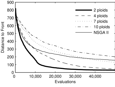
(a) 3 objectives

(b) 4 objectives

Figure 3.10: Convergence speed for DTLZ1

Table 3.5 shows the diversity of the algorithms after 50,000 function evaluations. NSGA-II has the highest diversity values in the case of 4, 6 and 10 objectives, while the 7-ploids algorithm outperforms the other algorithms in the 3 objectives problem. The diversity of the Polyploid algorithms is slightly increasing with increasing the number of objectives. A diversity value of 0.65 for the 2-ploids algorithm in 3 objectives reaches 0.79 in the 10 objectives case.

Table 3.6 shows the convergence of the algorithms after 50,000 function evaluations. The 2- ploids algorithm outperforms all the other algorithms in the 3, 4, and 6 objectives, while in the 10 objectives case, the 4-ploids algorithm is the best achieving a distance of 382 compared to 389 for the 2-ploids which comes second.

By comparing the Polyploid algorithms performance regarding the two performance criteria (convergence speed and diversity maintenance); increasing the ploidy number slightly increases the diversity of most Polyploid algorithms (maximum increase = 0.0618). On the other hand, a higher ploidy number slows down the convergence speed.

Table 3.5: Diversity after 50,000 function evaluations for DTLZ1

		objectives
algorithm	measure	3	4	6	10
2-ploids	Average	0.6506	0.6863	0.7067	0.7942
	Std. Dev.	0.0002	0.0003	0.0002	0.0003
4-ploids	Average	0.7065	0.7075	0.7043	0.7907
	Std. Dev.	0.0004	0.0001	0.0005	0.0001
7-ploids	Average	0.7124	0.7141	0.7480	0.8036
	Std. Dev.	0.0002	0.0002	0.0002	0.0003
10-ploids	Average	0.6993	0.6953	0.7201	0.8198
	Std. Dev.	0.0003	0.0001	0.0003	0.0001
NSGA-II	Average	0.6916	0.7945	0.9312	0.8722
	Std. Dev.	0.0914	0.0312	0.0195	0.0099

Table 3.6: Convergence after 50,000 function evaluations for DTLZ1

		objectives
algorithm	measure	3	4	6	10
2-ploids	Average	30.370	78.380	351.08	389.06
	Std. Dev.	0.0785	0.0782	0.2550	0.3853
4-ploids	Average	44.550	95.390	418.80	382.07
	Std. Dev.	0.1756	0.0828	0.3139	0.1801
7-ploids	Average	127.96	129.97	447.77	426.67
	Std. Dev.	0.1571	0.1657	0.1966	0.1564
10-ploids	Average	201.45	167.09	466.41	414.77
	Std. Dev.	0.3229	0.0905	0.2295	0.0647
NSGA-II	Average	157.00	219.09	442.94	485.17
	Std. Dev.	12.090	9.4720	25.340	3.6930

3.4.5 DTLZ2

The second benchmark problem to be used is DTLZ2, which is shown in (3.28) and (3.29).

$$\left.\begin{aligned} \text{Minimize}&&&f_{1}(\text{\bf x})=(1+g(\text{\bf x}_{M}))\cos(x_{1}\frac{\pi}{2})\cos(x_{2}\frac{\pi}{2})\dotsm\cos(x_{M-2}\frac{\pi}{2})\cos(x_{M-1}\frac{\pi}{2}),\\ \text{Minimize}&&&f_{2}(\text{\bf x})=(1+g(\text{\bf x}_{M}))\cos(x_{1}\frac{\pi}{2})\cos(x_{2}\frac{\pi}{2})\dotsm\cos(x_{M-2}\frac{\pi}{2})\sin(x_{M-1}\frac{\pi}{2}),\\ \text{Minimize}&&&f_{3}(\text{\bf x})=(1+g(\text{\bf x}_{M}))\cos(x_{1}\frac{\pi}{2})\cos(x_{2}\frac{\pi}{2})\dotsm\sin(x_{M-2}\frac{\pi}{2}),\\ \vdots&&&\vdots\\ \text{Minimize}&&&f_{M-1}(\text{\bf x})=(1+g(\text{\bf x}_{M}))\cos(x_{1}\frac{\pi}{2})\sin(x_{2}\frac{\pi}{2}),\\ \text{Minimize}&&&f_{M}(\text{\bf x})=(1+g(\text{\bf x}_{M}))\sin(x_{1}\frac{\pi}{2}),\\ \text{subject to}&&&0\leq x_{i}\leq 1,\quad\text{for}\;i=1,2,\dotsc,n.\end{aligned}\right\}$$ (3.28)

$$g(\text{\bf x}_{M})=\sum_{x_{i}\in\text{\bf x}_{M}}(x_{i}-0.5)^{2}.$$ (3.29)

Where x and $x_{i}$ are a decision vector and a decision variable, respectively. The function $g(\text{\bf x}_{M})$ requires $|\text{\bf x}_{M}|=k$ variables, and the total number of variables is $n=k+M-1$, where $M$ is the number of objectives.

The PF of this problem corresponds to $x_{i}^{*}=0.5$, ($x_{i}\in\text{\bf x}_{M}$) which leads to $g(\text{\bf x}_{M})=0$ and $\sum_{m=1}^{M}(f_{m}^{*})^{2}=1$. For this problem, the number of decision variables is set to $n=30$.

Figure 3.11 shows the distance to PF achieved by the algorithms against function evaluations. As with the case of DTLZ1, the 2-ploids algorithm is the best performer. It is converging faster than the other algorithms used. However, the performance of the optimizers get closer as the number of objectives increase. In the case of 10 objectives (Figure 3.11c) the 10-ploids algorithm overcomes the 7-ploids algorithm after 10,000 function evaluations. Figure 3.11a–LABEL:sub@fig:EA_poly_DTLZ2_conv_10 shows how the performance of NSGA-II is deteriorating by increasing the number of objectives, that in the case of 10 objectives the algorithm is diverging (Figure 3.11c).

(a) 3 objectives

(b) 4 objectives

(c) 10 objectives

Figure 3.11: Convergence speed for DTLZ2

Table 3.7 shows the diversity of the different algorithms. Although NSGA-II achieved the best diversity values in the 3, 4, 6 objective problems, its performance is declining with increasing the number of objectives. On the other hand, the performance of the Polyploid algorithms is either steady or improving with increasing the number of objectives. In the 3 objectives case, NSGA-II has a superior diversity value of 0.799, while the 7-ploids algorithm achieves a lower diversity value of 0.6452. But for the 10 objectives problem, the 7-ploids algorithm overcomes NSGA-II by achieving a value of 0.7398 while NSGA-II achieves 0.7194.

Table 3.7: Effect of varying ploidy number on diversity for DTLZ2

		objectives
algorithm	measure	3	4	6	10
2-ploids	Average	0.6621	0.6594	0.6263	0.6872
	Std. Dev.	0.0208	0.0744	0.0543	0.0721
4-ploids	Average	0.6622	0.6539	0.6610	0.7198
	Std. Dev.	0.0114	0.0212	0.0416	0.0492
7-ploids	Average	0.6452	0.6807	0.6773	0.7398
	Std. Dev.	0.0432	0.0229	0.0175	0.0115
10-ploids	Average	0.5865	0.6459	0.6881	0.7153
	Std. Dev.	0.0449	0.0229	0.0232	0.0338
NSGA-II	Average	0.7997	0.7750	0.7479	0.7194
	Std. Dev.	0.0148	0.0159	0.0109	0.0082

As shown in Figure 3.12a,LABEL:sub@fig:EA_poly_DTLZ2_PF_2side, the 2-ploids algorithm converged well to the PF of the 3 objectives problem, while NSGA-II stood at a relatively larger distance from that front as shown in Figure 3.12c.

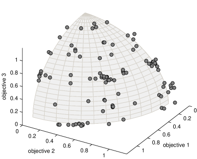
(a) 2-ploids

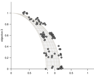
(b) 2-ploids (side view)

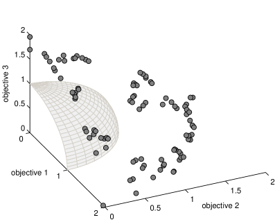
(c) NSGA-II

Figure 3.12: Obtained PF for DTLZ2 with $n=40$

The relative performance of the Polyploid algorithms in the DTLZ2 test problem is similar to that of the DTLZ1 test problem. Regarding diversity, increasing the ploidy number slightly affects the diversity of the Polyploid algorithms. The maximum change in diversity values is a decrease in the diversity of the 2-ploids algorithm by 0.0756, while the other Polyploid algorithms almost maintained a constant diversity value. Regarding convergence, increasing the ploidy number always slows down convergence, except for the 7 and 10-ploids algorithms in the 10 objectives problem as pointed out earlier.

To analyze the performance of the redundant chromosomes the following experiments are conducted. A new population is created by extracting all chromosomes in each solution vector in the Polyploid algorithms. This new population has a size of $N\times d$ , where $N$ is the original population size and $d$ is the ploidy number. Then the average distance of the new population to the PF is calculated, and the percentage of the dominated solutions in the new population is evaluated. For each of the Polyploid algorithms in Table 3.8, the first row shows the average distance of the original population to the PF. The second row shows the average distance of the new population to the PF. The third row shows the percentage of dominated solutions in the new population (using Pareto dominance).

Table 3.8: Performance of the extracted population

	distance	objectives
algorithm	to front	3	4	6	10
	original pop.	0.0515	0.1139	0.4381	0.9738
2-ploids	new pop.	0.0518	0.1145	0.4428	0.9929
	%dominated	7.52	6.25	4.89	2.11
	original pop.	0.0871	0.1469	0.7348	1.3115
4-ploids	new pop.	0.0890	0.1499	0.7528	1.3463
	%dominated	19.64	13.57	10.31	3.105
	original pop.	0.1402	0.2692	0.9319	1.6890
7-ploids	new pop.	0.1484	0.2785	0.9919	1.7293
	%dominated	40.17	20.55	13.43	3.26
	original pop.	0.3402	0.3358	1.2231	1.4619
10-ploids	new pop.	0.5006	0.3685	1.3160	1.4983
	%dominated	70.36	36.67	18.52	5.08

As shown Table 3.8, the average distance of the new population is slightly worse than that of the original population. In the case of 2-ploids algorithm with 3 objectives, the average distance is 0.0515 for the original population and it is 0.0518 for the new population. But in the case of 10-ploids algorithm with 3 objectives, the average distance deteriorates from 0.34 to 0.5. Note that the percentage of dominated solutions is low in the case of 2-ploids algorithm with a maximum value of 7.52% for the 3 objectives case. This value is steadily increasing with increasing the ploids number in all objectives cases reaching 70.36% dominated solutions for the 10- ploids algorithm with 3 objectives.

The new population which offers $N(d-1)$ more solutions may be used instead of the original population for the 2-ploids algorithm giving the decision maker more choices. It can be used in problems with high cost of function evaluations, as the $N(d-1)$ extra solutions are produced without any extra computational cost.

3.4.6 DTLZ3

The DTLZ3 problem is given as follows:

$$\left.\begin{aligned} \text{Minimize}&&&f_{1}(\text{\bf x})=(1+g(\text{\bf x}_{M}))\cos(x_{1}\frac{\pi}{2})\cos(x_{2}\frac{\pi}{2})\dotsm\cos(x_{M-2}\frac{\pi}{2})\cos(x_{M-1}\frac{\pi}{2}),\\ \text{Minimize}&&&f_{2}(\text{\bf x})=(1+g(\text{\bf x}_{M}))\cos(x_{1}\frac{\pi}{2})\cos(x_{2}\frac{\pi}{2})\dotsm\cos(x_{M-2}\frac{\pi}{2})\sin(x_{M-1}\frac{\pi}{2}),\\ \text{Minimize}&&&f_{3}(\text{\bf x})=(1+g(\text{\bf x}_{M}))\cos(x_{1}\frac{\pi}{2})\cos(x_{2}\frac{\pi}{2})\dotsm\sin(x_{M-2}\frac{\pi}{2}),\\ \vdots&&&\vdots\\ \text{Minimize}&&&f_{M-1}(\text{\bf x})=(1+g(\text{\bf x}_{M}))\cos(x_{1}\frac{\pi}{2})\sin(x_{2}\frac{\pi}{2}),\\ \text{Minimize}&&&f_{M}(\text{\bf x})=(1+g(\text{\bf x}_{M}))\sin(x_{1}\frac{\pi}{2}),\\ \text{subject to}&&&0\leq x_{i}\leq 1,\quad\text{for}\;i=1,2,\dotsc,n.\end{aligned}\right\}$$ (3.30)

$$g(\text{\bf x}_{M})=100\left[|\text{\bf x}_{M}|+\sum_{x_{i}\in\text{\bf x}_{M}}(x_{i}-0.5)^{2}-\cos(20\pi(x_{i}-0.5))\right].$$ (3.31)

Where x and $x_{i}$ are a decision vector and a decision variable, respectively. The function $g(\text{\bf x}_{M})$ requires $|\text{\bf x}_{M}|=k$ variables, and the total number of variables is $n=k+M-1$, where $M$ is the number of objectives.

This problem combines some of the properties of DTLZ1 and DTLZ2. It has a spherical PF like DTLZ2, and a huge number of local optima like DTLZ1. The PF is achieved at $x_{i}^{*}=0.5$ leading to $g(\text{\bf x}_{M}^{*})=0$. For this problem, the number of decision variables is set to $n=30$ and the optimizers were allowed to go for 50,000 function evaluations.

As shown in Figure 3.13, NSGA-II is converging well in early evaluations, and is overcome by the Polyploid algorithms one after the other, except the 10-ploids algorithm that gets very close to it after 50,000 evaluations. The 2-ploids algorithm is the fastest converging algorithm in all problems except for the 3 objectives problem where the 4-ploids algorithm catches it after around 20,000 evaluations.

(a) 3 objectives

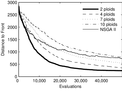
(b) 4 objectives

Figure 3.13: Convergence speed for DTLZ3

Regarding diversity, as shown in Table 3.9, NSGA-II achieves the best values for the 4, 6, and 10 objectives problems. It has a value of 0.7399 in the 6 objectives problem followed by the 10-ploids algorithm with a value of 0.5994. However NSGA-II has the worst diversity for the 3 objectives problem with a value of 0.4665, and the second worst is the 10-ploids algorithm with 0.5144 diversity value.

Table 3.9: Diversity after 50,000 function evaluations for DTLZ3

		objectives
algorithm	measure	3	4	6	10
2-ploids	Average	0.6158	0.5944	0.4768	0.6279
	Std. Dev.	0.0004	0.0005	0.0004	0.0010
4-ploids	Average	0.6380	0.5504	0.5312	0.6736
	Std. Dev.	0.0005	0.0004	0.0005	0.0008
7-ploids	Average	0.5753	0.5419	0.5554	0.7059
	Std. Dev.	0.0008	0.0004	0.0006	0.0004
10-ploids	Average	0.5144	0.5940	0.5994	0.6784
	Std. Dev.	0.0003	0.0003	0.0006	0.0007
NSGA-II	Average	0.4665	0.6217	0.7399	0.7271
	Std. Dev.	0.0022	0.0002	0.0004	0.0002

As shown in Table 3.10, the 2-ploids algorithm, again, achieves the best convergence values in the 4, 6 and 10 objectives problems. The 4-ploids algorithm is the best for the 3 objectives problem as it reaches a distance to the PF of 115.5 followed by the 2-ploids algorithm with a distance of 141.1. The effect of increasing the ploidy number in this test problem is little higher than DTLZ1 and DTLZ2. Regarding diversity, the performance of the 3 objectives problem decreases by 0.1014 when the ploidy number increases from 2 to 10, while the performance of the 4 objectives problem remained the same and the 6 and 10 objectives problems have an increase of 0.1226 and 0.0505, respectively, for the same increase in ploidy number. Regarding convergence, increasing the ploidy number slows down convergence in all problems except for the 2 and 4-ploids algorithms in the 3 objectives problem as pointed out earlier.

Table 3.10: Convergence after 50,000 function evaluations for DTLZ3

		objectives
algorithm	measure	3	4	6	10
2-ploids	Average	141.10	242.48	944.94	2363.3
	Std. Dev.	0.3452	0.2461	1.4432	1.7410
4-ploids	Average	115.50	350.82	1137.7	2426.3
	Std. Dev.	0.3571	0.4869	2.4923	1.0542
7-ploids	Average	191.24	546.10	1499.5	2393.6
	Std. Dev.	0.5813	0.6889	1.7420	1.1733
10-ploids	Average	436.78	784.23	1669.1	2490.1
	Std. Dev.	0.8684	0.9927	0.8052	1.4455
NSGA-II	Average	396.20	712.24	2328.5	3124.5
	Std. Dev.	0.6275	0.5085	1.4124	0.9903

3.4.7 DTLZ4

The DTLZ4 test problem is defined as follows:

$$\left.\begin{aligned} \text{Minimize}&&&f_{1}(\text{\bf x})=(1+g(\text{\bf x}_{M}))\cos(x_{1}^{\alpha}\frac{\pi}{2})\cos(x_{2}^{\alpha}\frac{\pi}{2})\dotsm\cos(x_{M-2}^{\alpha}\frac{\pi}{2})\cos(x_{M-1}^{\alpha}\frac{\pi}{2}),\\ \text{Minimize}&&&f_{2}(\text{\bf x})=(1+g(\text{\bf x}_{M}))\cos(x_{1}^{\alpha}\frac{\pi}{2})\cos(x_{2}^{\alpha}\frac{\pi}{2})\dotsm\cos(x_{M-2}^{\alpha}\frac{\pi}{2})\sin(x_{M-1}^{\alpha}\frac{\pi}{2}),\\ \text{Minimize}&&&f_{3}(\text{\bf x})=(1+g(\text{\bf x}_{M}))\cos(x_{1}^{\alpha}\frac{\pi}{2})\cos(x_{2}^{\alpha}\frac{\pi}{2})\dotsm\sin(x_{M-2}^{\alpha}\frac{\pi}{2}),\\ \vdots&&&\vdots\\ \text{Minimize}&&&f_{M-1}(\text{\bf x})=(1+g(\text{\bf x}_{M}))\cos(x_{1}^{\alpha}\frac{\pi}{2})\sin(x_{2}^{\alpha}\frac{\pi}{2}),\\ \text{Minimize}&&&f_{M}(\text{\bf x})=(1+g(\text{\bf x}_{M}))\sin(x_{1}^{\alpha}\frac{\pi}{2}),\\ \text{subject to}&&&0\leq x_{i}\leq 1,\quad\text{for}\;i=1,2,\dotsc,n.\end{aligned}\right\}$$ (3.32)

$$g(\text{\bf x}_{M})=\sum_{x_{i}\in\text{\bf x}_{M}}(x_{i}-0.5)^{2}.$$ (3.33)

Where x and $x_{i}$ are a decision vector and a decision variable, respectively. The function $g(\text{\bf x}_{M})$ requires $|\text{\bf x}_{M}|=k$ variables, and the total number of variables is $n=k+M-1$, where $M$ is the number of objectives.

The PF for this problem is attained when $x_{i}^{*}=0.5$, leading to $g(\text{\bf x}_{M})=0$. This problem is a modified version of DTLZ2 with a different meta-variable mapping ($x\to x^{\alpha}$). This mapping allows a dense set of solutions near the $f_{M}-f_{1}$ planes [85]. This biased distribution of solutions attracts the algorithms to produce more solutions in the $f_{M}-f_{1}$ planes and makes it difficult for them to maintain a good distribution. For this problem, then number of decision variables is set to $n=30$, while $\alpha=100$ as suggested in [85].

Figure 3.14 shows the convergence of the algorithms in the 6 and 10 objectives problems. The 2-ploids algorithm is the fastest converging algorithm, again, and is followed by the 4-ploids algorithm, while the NSGA-II is the slowest converging algorithm and diverges in the 6 and 10 objectives problems. As shown in Table 3.11, NSGA-II achieves the best diversity values for the 3, 6 and 10 objectives problems, and comes third in the 4 objectives problems after the 10 and 7-ploids algorithms, respectively. NSGA-II achieves much better diversity value in the 10 objectives problem than any of the Polyploid algorithms. It achieves a diversity value of 0.7668 followed by a diversity value of 0.2763 for the 10-ploids algorithm.

(a) 6 objectives

(b) 10 objectives

Figure 3.14: Convergence speed for DTLZ4

Table 3.11: Diversity after 50,000 function evaluations for DTLZ4

		objectives
algorithm	measure	3	4	6	10
2-ploids	Average	0.5956	0.6101	0.4946	0.1754
	Std. Dev.	0.0010	0.0003	0.0005	0.0005
4-ploids	Average	0.6517	0.6487	0.5634	0.1866
	Std. Dev.	0.0002	0.0008	0.0002	0.0005
7-ploids	Average	0.6634	0.6926	0.5746	0.2618
	Std. Dev.	0.0002	0.0002	0.0002	0.0004
10-ploids	Average	0.6711	0.6986	0.6087	0.2763
	Std. Dev.	0.0003	0.0002	0.0002	0.0004
NSGA-II	Average	0.7320	0.6870	0.6970	0.7668
	Std. Dev.	0.0003	0.0003	0.0002	0.0002

The low diversity values for the Polyploid algorithms in the 10 objectives problem compared to that of NSGA-II reflects its failure to maintain a good diversity of solutions in problems with non-uniform distribution of solutions along the PF, coupled with a high number of objectives (10 objectives).

Table 3.12 shows that all Polyploid algorithms have better convergence values than NSGA-II, except for the case of 10-ploids with 3 objectives case. In this case the 10-ploids reaches a distance of 0.2239 to the PF compared to a value of 0.1759 for NSGA-II. The 2-ploids algorithm achieves the best convergence values at the end of the 50,000 function evaluations except for the 4 objectives problem where it achieves a value of 0.0587 and comes second to the 4-ploids algorithm which reaches a distance of 0.0547 to the PF.

Table 3.12: Convergence after 50,000 function evaluations for DTLZ4

		objectives
algorithm	measure	3	4	6	10
2-ploids	Average	0.0249	0.0587	0.0529	0.6421
	Std. Dev.	0.0001	0.0002	0.0001	0.0032
4-ploids	Average	0.0359	0.0547	0.1069	0.6778
	Std. Dev.	0.0001	0.0001	0.0003	0.0027
7-ploids	Average	0.0748	0.0967	0.1431	1.1748
	Std. Dev.	0.0002	0.0003	0.0003	0.0012
10-ploids	Average	0.2239	0.1241	0.2654	1.1822
	Std. Dev.	0.0008	0.0003	0.0008	0.0017
NSGA-II	Average	0.1759	0.7957	3.7163	5.1274
	Std. Dev.	0.0011	0.0032	0.0029	0.0029

Diversity values are steadily, though slightly, increasing in all problems with increasing the ploidy number. The convergence performance on the other hand is negatively affected by increasing the ploidy number. The average distance to the PF is steadily increasing with increasing the ploidy number except for the 2 and 4-ploids cases in the 4 objectives problem as pointed out earlier.

3.4.8 Conclusion

The benchmark problems used tested the performance of the Polyploid algorithms and the NSGA-II algorithm regarding convergence to the PF and the diversity of the obtained solutions. The first three test problems (DTLZ1–3), which emphasize convergence, showed the ability of the Polyploid algorithms to converge faster than NSGA-II to the PF, however, the convergence speed decreased as the ploidy number increased. On the other hand, an increase in the ploidy number resulted in a slight improvement regarding diversity of solutions in problems with higher number of objectives (6, 10 objectives). This slight improvement almost vanished for problems with lower number of objectives (3, 4 objectives). The fourth test problem (DTLZ4) tested the ability of the algorithms to maintain a good distribution of solutions across the PF. The Polyploid algorithms maintained a reasonable degree of diversity but lower than that of the NSGA-II algorithm in the 3, 4, and 6 objectives problems. However, they failed to maintain a satisfactory degree of diversity in the 10 objectives problem compared to the diversity obtained by the NSGA-II algorithm.

Although an increase in the ploidy number generally resulted in a slight improvement in diversity values, this marginal benefit was accompanied by a decrease in convergence speed overshadowing the diversity enhancement. Based on the obtained results, a ploidy number between 2 and 4 is recommended for obtaining a good convergence speed while not sacrificing diversity.

Chapter 4 Swarm Intelligence Methods

4.1 Introduction

Not long time ago, man dreamed of a computing machine that could do his time consuming and tiresome mathematical calculations. Although man did not know how exactly this machine will look like or operate, he expected that this machine will be like human brain, capable of reasoning and solving problems just like humans do, or even better.

When the first models of this computing machine started to appear, researchers and philosophers started arguing about the effects that these new computing machines or computers will have on mankind. Some of them were doubtful about their widespread, and usability, while others anticipated that these infallible machines will control the human race. It did not take much time until scientists and researchers realized the big differences between the human brain and these computers. Those computers cannot recognize a face or understand spoken language, although these are easy tasks for a four years old child.

Some researchers believed that the best way to resemble human ability of solving problems is to create a model of his brain and use it in solving problems. They created ANNs, which are loose models of the cortical structures of the brain. ANNs were relatively successful in some applications such as pattern recognition compared to other techniques preceded it, but yet failed to achieve the feats that human brain can do, because they are not intelligent. But what is intelligence?

There is no common definition for intelligence or what are the properties of an intelligent entity. Sometimes it is defined using a set of qualities such as the verbal, analytical, problem-solving and reasoning abilities, among others, while according to Edwin G. Boring: intelligence is whatever it is that an intelligence test measures. Alan Turing defined intelligence as the ability to pass a test he proposed [86]. In this test, a judge sits in a room and makes a conversation in writing with a man and a machine in another room without seeing or hearing them. If the judge cannot identify or wrongfully identifies the man or the machine, then this machine is considered intelligent.

The Turing definition of intelligence is unique in the sense that it includes a social aspect; An intelligent machine should be able to understand and distinguish different meanings of a word according to the context of the conversation. It can feel the tone of the language and distinguish a joke from a serious speech.

Many researchers accepted Turing’s definition of intelligence and started investigating social interactions of different species. Their views and findings were quite interesting.

Some researchers investigating the social behaviors of bees concluded that the beehive is a single living creature, just as a man, and a bee is only a part or an organ of this creature, just as a nail or an eye to a man. The simple brain of a single bee does not allow it to build the complex structured beehive, find food, and protect the hive. But the collective behavior of the entire swarm manages to do all this. It is to be noted that the collective behavior of the swarm is not a sum of the parts; rather it is a behavior that emerges due to social interaction between parts of the system.

The behavior of many insects, birds and fish was fascinating and inspiring. After noticing that a swarm of ants can find the shortest route from the nest to a piece of food, researchers created a model that copies the behavior of this swarm to find the shortest route for the TSP [87]. In another observation, researchers managed to build a computer paradigm which mimics the behavior of a flock of birds searching for food [88]. This paradigm has strong ability to find the optimum value of a function just like the ability of a bird flock in finding food.

Swarm Intelligence (SI) methods are optimization techniques which are based on the collective behavior in decentralized, self-organized systems, comprising relatively simple agents equipped with limited communication, computations and sensing abilities [89, 90, 91].

James Kennedy and Russell Eberhart proposed extending the conventional definition of a swarm to include any such loosely structured collection of agents interacting in a space (not necessarily a physical space) which may allow the existence of more than one agent at the same position (such as the cognitive space where collision is not a concern) [92].

The most widely known and used SI methods are ACO and PSO, though there are other techniques that fall under the SI umbrella such as the Stochastic Diffusion Search (SDS) method [93].

4.2 How and Why They Work?

SI methods work differently, so there is no global answer to the question “How SI methods work?”.

ACO works by simulating a colony of ants searching for food. Each ant leaves a pheromone trail whenever it walks, and this trail evaporates gradually over time. However, an ant passing over an old trail will leave its pheromone over that trail, leading to accumulation of pheromone and consequently a stronger pheromone trail. If an ant ran into a crossroad, it will choose the one which has the strongest pheromone trail. This mechanism leads to the emergent behavior which helps the ant colony find the shortest route to food.

As shown in Figure 4.1, ‘a-b-d’ and ‘a-c-d’ are two possible routes between the nest and a food source. Ants initially choose a random route, so it will be equally probably that an ant chooses any of the two routes. However, the ants taking the first route ‘a-b-d’ will make more trips between the nest and the food source in a given time, than those taking the second route ‘a-c-d’. Henceforth, the pheromone trail on the first route will gradually become stronger than that of the second route, and because ants tend to choose the route with the strongest pheromone trail, the probability that an ant chooses the first route will increase over time. As more ants choose the first route, the stronger its pheromone trail becomes and the more ants will prefer it. On the other hand, the pheromone trail on the second route gradually evaporates, and as long as the ants keep switching to the first route and reinforcing it on the expense of the second one, the pheromone trail on second route will get weaker and weaker. Eventually, almost all the ants will go through the first route which optimizes their travel distance.

Figure 4.1: Swarm of ants find the shortest route from nest to food

The ACO algorithm can be used to solve the TSP [94], where the cost of traveling between two cities is equivalent to part of the tour length the ants take from the nest to the food source. Analogously, it can be used for scheduling problems and many combinatorial optimization problems as well [95, 96].

The way that the PSO algorithm works will be explained in detail in Section 4.3.

Despite few theoretical analysis of some SI techniques [97, 98, 99, 92], the answer to “Why SI methods work?” is still unclear. The complexity of the behavior that emerges from simple social interactions among swarm members makes the mathematical analysis of such models quite hard. It was noted that SI methods are simple to implement but are hard to understand [100]. This may explain the tendency of most researchers to conduct empirical rather than theoretical studies [101].

4.3 Particle Swarm Optimization

The first models of a flying flock of birds were created for animation purposes, so it was mainly about high aesthetic animation rather than solving a problem. Craig Reynolds created a powerful simulation of flocking birds. His swarm of Boids (artificial birds) was driven by three simple rules so that each swarm member would avoid collision, match its velocity with other swarm members, and move to the swarm center as it perceive it [102]. The realistic animation this algorithm produced, which was driven by three simple rules, encouraged other researchers to follow Reynolds. Frank Heppner and Ulf Grenander analyzed the films they recorded for flocking birds and created a powerful computer simulation of artificial birds. Their rules were similar to those set by Reynolds though there were some differences.

Two researchers, James Kennedy, a social psychologist, and Russell Eberhart, an electrical engineer, were inspired by the work of Reynolds and Heppner [92] though they perceived it differently—influenced by their areas of research. They created a computer paradigm which simulates a flock of flying birds. Their paradigm shares the same theme of Reynolds’ and Heppner’s work in the sense that there was no central control over the swarm, however their paradigm was more simple and had different set of rules. Unlike their predecessors, Kennedy and Eberhart proposed applications outside computer graphics field. They proposed using their algorithm in simulating and studying social interactions of different societies, be it human or animal societies. In the same paper [88], they used their paradigm in solving an engineering problem. It was used in training an ANN. Because their computer simulations of flocking birds looked more like particles on computer screen than real birds, the collision avoidance rules were removed, the flock turned into a swarm, and due to the applicability of their algorithm in optimization problems, Kennedy and Eberhart called their paradigm “Particle Swarm Optimization”.

After many experiments and modifications, the first PSO model [88] was built on a population of agents or particles. Each particle occupies a point in the $n$-dimensional solution space, which makes it a potential solution vector. The algorithm initializes by assigning each particle a random position and velocity vectors. As the particles fly in the solution space, three forces act upon them. The first one is an inertia which helps each particle maintain its current direction and velocity. The second force pushes each particle towards the best position it found in the past (personal best pbest), while the third one pushes each particle towards the best position found by all the particles of the swarm (global best gbest). It is to be noted that the second and third forces are directly proportional to the distance between current position of the particle from one side, and pbest and gbest positions from the other side, respectively. The effect of these forces on the velocity of the particles can be described by the following equation:

$$\begin{split}v_{id}(t+1)=&v_{id}(t)+\\ &2\times rand_{1}\times(p_{id}(t)-x_{id}(t))+\\ &2\times rand_{2}\times(p_{gd}(t)-x_{id}(t))\end{split}$$ (4.1)

Where

• $v_{id}(t+1)$ is the $d$ velocity component of particle $i$ at time $t+1$,

• $rand_{1}$ and $rand_{2}$ are two independent random numbers in the range $(0,1)$,

• $p_{id}$ is the $d$ component of the best position found by particle $i$ (pbest position),

• $p_{gd}$ is the $d$ component of the best position found by all swarm members (gbest position), and

• $x_{id}(t)$ is the $d$ position component of particle $i$ at time $t$.

At each time step the position of each particle is updated according to the following rule:

$$x_{id}(t+1)=x_{id}(t)+v_{id}(t+1)$$ (4.2)

As the particles fly in the solution space, they are pushed by their inertia to explore new regions, while the second and third components of (4.1) work together to help the particles converge to the global, or a good local optimum solution. A weight value of 2 multiplied by a random number with a mean value of 0.5 means that the particles will overfly the target about half the time [88], and will eventually converge and land over an optimum solution.

A Matlab code describing a simple PSO algorithm is presented below for a minimization problem:

A simple PSO algorithm (Matlab code)

⬇

initialize(x, v, t); % initialize parameters;

% x => position,

% v => velocity.

while (termination == 0)

gbest = inf; % gbest => global best.

for i = 1 : swarm_size

fitness(i) = evaluate(x(i, :)); % evaluate fitness.

if (fitness(i) < pbest(i)) % if better than pbest,

pbest(i) = fitness(i); % store the new value,

pl(i, :) = x(i, :); % and update pbest.

if (fitness(i) < gbest) % if better than gbest,

gbest = fitness(i); % store the new value,

pg = i; % and update gbest.

end

end

end

v = v + 2*rand*(x - pl) + 2*rand*(x - pl(pg, :));

% update velocity,

x = x + v; % and position.

t = t + 1; % increment counter.

termination = term_check(x, v, t);% termination check.

end

4.3.1 Spaces of the Algorithm

Kennedy has worked out an analysis of the PSO algorithm which was greatly influenced by his social psychological experience. He used a swarm of humans instead of the systematic use of birds. This replacement of characters by itself added strength to his argument for three reasons: i) it overcomes the conventional depiction of PSO models as a swarm of birds and presents a new example to evoke the imagination of other researchers. ii) the choice of humans allows him to apply the results obtained by decades of social psychology research in AI context. iii) the examples used were clear because they touch the social life experience of humans. In his analysis, a man is subjected to various stimuli by his environment from which he learns affected by other individuals trying to reach a point that achieves their maximum satisfaction. This analysis was derived based on a three dimensional space; The parameters space, the sociometric space, and the evaluative space [100].

The Parameters Space

The parameters space simply is the solution space or the decision space. It is made-up of the problem parameters which when correctly tuned, the global optimum solution is attained. These parameters can be perceived as the variables of mind. They determine how the mind processes information and reacts to different stimuli in its environment. They are complex and interwoven in the sense that a change in the value of one variable affects many objectives in most practical problems. This complexity is analogous to epistasis in GAs.

The variables of mind, such as beliefs and norms, may change as man learns and acquires experience in the course of his life. A man is influenced by his environment, past experience, and the experience of his neighbors with whom he interacts, among other influences.

The environment may influence a man by limiting his choices, so he may not tune his mind variables to his satisfaction, such as an oppressive society that persecutes people holding certain beliefs. The environment in this case adds constraints on the variables.

Personal experience is very influential in people’s life. Man tends to remember the most successful experiences in his life, and when a situation repeats, he recalls the action which lead to the most satisfactory result (according to his standards) for that situation in the past, and tends to repeat this action or try a similar one. The action which caused the most satisfactory result is represented by $p_{id}$ in (4.1).

Another major source of influence for humans is the experience of their neighbors. The definition of neighborhood will be explained in detail in Subsection 4.4.3, but for now it is enough to say that the neighbors of an individual are those individuals who are at certain degree of closeness to him. A man tends to imitate or resemble his most successful neighbor, believing that by taking the same action, he will get a similar successful result. This imitation may come in handy in many situations; Scientific research in fact is heavily based on this kind of imitation, a researcher reads about the work of other researchers and have discussions with them to learn from their experience. The action which caused the most successful result among all individuals in a man’s neighborhood is represented by $p_{gd}$ in (4.1).

It is to be noted that learning occurs at a slower pace than perceiving information. Although there is an overwhelming volume of information that pours into man’s mind every day, the states of his mind do not change in reaction to each piece of this information. The rate at which he is affected by these stimuli is known as the learning rate, which will be explained in Subsection 4.4.1.

The Sociometric Space

The sociometric space is among the properties which distinguish PSO from EAs. In this space, the particles’ neighborhood is defined and directly affects the interactions among different particles and how they will learn from each other. Every man gets influenced by his neighbors, but practically, this influence depends on many factors. Kennedy defined three factors affecting this influence [100]:

1. Strength: is a relative measure of how much a man is attracted to the neighbor in a certain situation. The strength of a neighbor could be a measure of his persuasiveness, social status, or a personal experience with that neighbor. In the PSO example given earlier, strength was measured by the fitness of the particle; a particle is affected by the most fit particle in its neighborhood.

2. Immediacy: is a measure of the degree of closeness to the neighbor. Closeness should not be associated exclusively with the physical space or the Euclidian sense. It could be the distance in a cognitive space: a man is affected by neighbors sharing his beliefs, or blood bond: a man is affected by his father who lives in another continent. The degree of closeness could be crisp (neighbor or not a neighbor), or fuzzy (varying gradually as distance changes). In the previous PSO example, immediacy was crisp and was limited by the neighborhood topology.

3. Number: is the number of neighbors sharing the same belief. This factor is not applicable in some situations; in real life, the beliefs and standards of people are spread along wide spectrum, it is really hard to find two people share the exact beliefs. Furthermore, if the fuzzy neighborhood definition is adopted, the classification of people as neighbors and not-neighbors will not be possible. The ‘number’ factor was not considered in the previous PSO example.

In real-world, influence is not symmetric. An idol has a far reaching influence on millions, but there is no reciprocal influence by those millions on that idol. A less drastic example is the mutual influence between a father and a son. So, the influence has to be defined in both directions. Moreover, things may get more complicated when realizing that some influences depend on others. The influence of a parent on his son could be drastically reduced if the two parents get separated, noting that the son was directly connected to both of them. Influence can be mutually interactive; $a$ trusts $b$ because $b$ trusts him.

The social networks greatly depend on people and environment. A solitary man is connected to much fewer people than a gregarious one, and a man living in a city hub will meet more people than a one living on the fringe of the city.

Neglecting the effect of time is not a wise choice. The social networks are highly dynamic, even if one tries hard to keep a connection, it could be broken from the other side, so a shrewd man may adjust his social network from time to time to his benefit.

The premise that an individual is affected by one neighbor is in fact not judicious. Although a neighbor could be more influential on a man than other neighbors, he does not block their influence on that man. In many situations, a man is affected by the norms and beliefs of his society which do not stem from a single individual or a bunch of people, and do not emerge a fortnight.

Although two people may not be directly connected, they could still influence each other through the neighbors they share, or the neighbors that their neighbors share. Obviously, this chain can go on and on, and its shape determines what is known as the flow of influence. The flow of influence determines, among other things, how fast the influence of a superior man will spread through people and affects them, and the direction or path of this spread. A good example is the spread of an epidemic disease, in this case, the spread of the virus depends on our social networks among other factors. The spread of influence is a mixed blessing, a rapid spread of influence means fast convergence, but to a local optimum in most cases. While a slow spread helps exploring the search space looking for the global optimum, and meandering in the meanwhile.

The Evaluative Space

The evaluative space is the space where all possible reactions to different stimuli is defined. This reaction is mainly based on the states of mind and is affected by noise. In the evaluation process, the input parameters of a $n$-dimensional space are mapped to a relative evaluation values in a one dimensional space, and based on their relative position along this dimension a decision is made. However this mapping could be misleading; such as the drag force of an object approaching the speed of sound. The drag force acting on this abject increases as its speed gets closer to the speed of sound, but once it reaches it, the drag force suddenly collapses. The mapping could be flat; like searching for the correct numbers combination to open a lock, there is no indication whatsoever to guide the search process towards the optimum solution.

Different stimuli are compared relative to each other on the one dimensional evaluative space. The absolute evaluation value of a stimulus is worthless, where does a 1000$ salary stands? It is high when compared to a 500$ pay, but a low one when compared to a 5000$ stipend. Does that make a 5000$ allowance a good one? Not when compared to a 7000$ one.

As time passes by and situations change, the comparison level changes as well. The comparison level, adaptation level, or anchor [100] is the reference level, which compared to it, the values of different stimuli are classified as satisfactory and non-satisfactory. Henceforth, a man who gets the highest salary in his firm may not be satisfied with it because he compares it to the higher salary he had at his previous position. But once his salary surpasses that old one, the adaptation level rises with it. The new adaptation level is the value of the higher salary, and a lower salary which was acceptable in the past will no longer become acceptable.

In the PSO example given in Section 4.3, the $n$-dimensional position of each particle (in the parameters space) was mapped to a one dimensional fitness value (in the evaluative space). The fitness value of each particle assigns it a position along the fitness scale to be relatively compared to other particles. While $p_{id}$ and $p_{gd}$ are the local and global adaptation levels , respectively, that a particle maintains. In this PSO algorithm, the order of a particle is all that matters; if a particle has the best local/global fitness value, this value becomes the local/global best with no regard to its absolute value, and with no regard to differences between this value and the values of other particles.

4.4 Variations

The basic PSO algorithm which was developed by Kennedy and Eberhart and was presented in their 1995 paper became obsolete. Different variations has been made to the algorithm either by those two researchers or by others when the algorithm was widely accepted few years after its embarkation. Different rates of learning were tested and proposed [103]. The inertia that help the particles maintain their direction were constricted [104]. Different social networks were tested and suggested [105, 106, 107, 108], and extension of the PSO algorithm was made to binary and discrete problems as well [109, 100, 92].

4.4.1 Learning Rates

The learning rates, or acceleration coefficients, are the parameters that determine the degree to which a particle is affected by its past experience and the experience of its neighbors. In the basic PSO algorithm, there was two such parameters, however their were set to a constant value of 2. In modern PSO implementations, these parameters ($\varphi_{1}$, $\varphi_{2}$) are introduced to the velocity update equation

$$\begin{split}v_{id}(t+1)=&v_{id}(t)+\\ &\varphi_{1}\times rand_{1}\times(p_{id}(t)-x_{id}(t))+\\ &\varphi_{2}\times rand_{2}\times(p_{gd}(t)-x_{id}(t))\end{split}$$ (4.3)

When $\varphi_{1}>\varphi_{2}$, the particle tends to rely on its past experience than the experience of its neighbors, and when $\varphi_{1}<\varphi_{2}$, the particle trusts the experience of its neighbors more than its own experience. Most PSO implementations use equal values for those two parameters ($\varphi_{1}=\varphi_{2}$). Maurice Clerc and Kennedy suggested setting those two parameters such that $\varphi_{1}+\varphi_{2}=4.1$ [110], however other researchers reported better results over a wide set of test function when those two parameters were set at other values [107, 111].

The summation of $\varphi_{1}$ and $\varphi_{2}$ affects the performance of the algorithm as well. As the value of $\varphi_{1}+\varphi_{2}$ increases, the particles increase their steering degree and become relatively less affected by the inertia force. The situation is like driving a moving car, $v_{id}$ is the velocity vector of the car, and $\varphi_{1}$, $\varphi_{2}$ are the degrees to which the driver steers the wheel to hit his target. As $\varphi_{1}$ and $\varphi_{2}$ increases, the driver steers his wheel more sharply towards pbest and gbest points, respectively, whenever he sees them, and consequently explores smaller portion of the landscape.

4.4.2 Constriction

It was found during early experiments on PSO that the velocity of the particles explode and approach infinity [100]. So, Kennedy and Eberhart set a maximum velocity limit on the movements of the particles $v_{max}$ to prevent this behavior, without understanding its causes. Eberhart and Shi [112] introduced an inertia weight to the algorithm ($w$). The velocity update equation became:

$$\begin{split}v_{id}(t+1)=&w\times v_{id}(t)+\\ &\varphi_{1}\times rand_{1}\times(p_{id}(t)-x_{id}(t))+\\ &\varphi_{2}\times rand_{2}\times(p_{gd}(t)-x_{id}(t))\end{split}$$ (4.4)

The weight $w$ is typically below the unity value, to act like damper for the velocity of the particle. When $w$ is close to a value of 1, the particles swing and meander in the search space, and have a high exploration power. While decreasing the value of $w$, inhibits the velocity of the particles and allows them to converge faster. They suggested starting the algorithm by a weight value of 0.9 to scout out the landscape, then reducing this value to exploit the obtained knowledge as the algorithm proceeds, till it reaches 0.4 at the end of the run.

Clerc and Kennedy worked out a mathematical analysis of the PSO algorithm in their award winning paper [110]. They explained the reasons which lead to explosion of the velocity of the particles and analyzed the particle’s trajectories as it moves in discrete time and developed a generalized model in a five-dimensional complex space with a set of coefficients to control the convergence of the algorithm. They suggested a constriction coefficient ($\chi$) to wight the entire right-hand side of the velocity update equation. It looked like

$$\begin{split}v_{id}(t+1)=&\chi\times(v_{id}(t)+\\ &\varphi_{1}\times rand_{1}\times(p_{id}(t)-x_{id}(t))+\\ &\varphi_{2}\times rand_{2}\times(p_{gd}(t)-x_{id}(t)))\end{split}$$ (4.5)

The value of $\chi$ is suggested to be approximately 0.729, and $\varphi_{1}+\varphi_{2}=4.1$.

4.4.3 Social Networks

The social network of the PSO algorithm is what mainly distinguishes it from other SI techniques, and more generally, from other CI methods. The basic PSO algorithm which was presented in Section 4.3 used a fully connected social network; every particle is connected to all other particles as shown in Figure 4.3, which means it is aware of their best fitness value and the position that resulted in this value. This social network is known as the gbest topology, where ‘g’ stands for ‘global’ because each particle is affected by the global best position. The gbest topology is known for its rapid convergence, and susceptibility to local optima as well. As soon as one particle finds a global best value early in the run, the other particles hurtle to it, and as long as those particles encounter improvements in their fitness values while approaching that global best, they get more strongly sucked towards it, and eventually, they all converge to this global best which happens to be a local optima in most practical problems. Henceforth, many other social networks were proposed to alleviate this shortcoming and to add more strength to the algorithm.

lbest

The lbest topology is one of the earliest topologies used. The ‘l’ in its name refers to ‘local’, because each particle is only connected to its ‘locals’. By other words, if the particles were arranged in a circle, each one will be connected to the particle that precedes it, and the one which succeeds it along the circle path as shown in Figure 4.3. Note that the neighborhood in the lbest topology is based on an arbitrary, but fixed, index values for the particles, and it has nothing to do with their inter-distances in the decision space or the objective space.

Due to lack of unique position attracting all swarm members, such as in gbest topology, a swarm connected using an lbest topology will be affected by different points of attraction. If a particle, or a group of particles get trapped in a local optima, their detrimental influence will spread slower than the case of the gbest topology, and it is likely that their neighbors will find a better value and pull them out of the trap.

Figure 4.2: gbest topology

Figure 4.3: lbest topology

Hierarchical PSO

Hierarchical PSO (H-PSO) is another PSO topology proposed by Stefan Janson and Martin Middendorf [107]. By using this topology, the particles are arranged in a hierarchy structure, and the neighborhood of each particle is made of the particle itself and its parent node in the hierarchy. The hierarchy is defined by its height ‘h’, and its branching degree ‘d’. For example, Figure 4.4 shows a swarm of 21 particles arranged in a hierarchy of height $h=3$, and a branching degree of $d=4$. However, it will not be possible to construct a regular tree for the particles with a uniform branching degree at all nodes. Henceforth, any inconsistency will be pushed to the inner nodes at the deepest level of the tree, and the maximum difference of branching between any of those irregular nodes will be at most one.

The fitness of each swarm member is evaluated as usual, then starting from the top of the tree and proceeding to the bottom, the local best fitness value of each swarm member represented by a parent node in the tree is compared to that of its child nodes in the hierarchy. If the parent is less fit than the best one of its child nodes, they swap their positions in the hierarchy, and if not, they stay at the same hierarchy position. This procedure pushes the more fit particles up in the tree, and drags the less fit down towards the bottom of the tree. As a result, the procedure will arrange the particles in the tree according to their fitness, with the most fit at the top of the tree, and the least fit at the bottom. Since the neighborhood of each particle consists of itself and its parent node, the more close a particle gets to the top of the tree, the larger its influence will become. Traversing the tree using a breadth-first procedure starting from the top of the tree allows a particle to move down the tree up to $h-1$ levels in a single iteration of the algorithm if it is worse enough, but limits the ascending speed to 1 level per iteration. This tree update procedure is repeated with every iteration of the PSO algorithm.

The PSO algorithm will continue as usual by updating the velocity of the particles using their local best and their neighbors’ best, and then updating their position in the decision space. The algorithm repeats by evaluating the fitness of these new positions, then traversing and updating the tree, following by a velocity and position update…and so on.

The philosophy of the H-PSO is almost the opposite of the C-PSO. H-PSO promotes the best particles and increases their influence in the swarm hopefully to speed up convergence, while the worst particles are dragged to the bottom of the tree to let them learn directly from particles which are the second worst after them. On the other hand, C-PSO topology reduces the influence of the best particles by inhibiting their social interaction with other particles, while allowing the worst particles to socialize more and increases their chance of learning directly from the best particles. H-PSO and C-PSO are similar in other facets, they both employ a dynamic neighborhood which adapts to the fitness or the particles, however they adapt differently.

Figure 4.4: Hierarchical PSO

Fitness Distance Ratio PSO

Fitness-Distance-Ratio PSO (FDR-PSO) is variant of the PSO which is based on a social network unique from those presented earlier. This topology which was proposed by Kalyan Veeramachaneni et al. [113], was inspired from the observation of animal behavior. An animal is most likely to be influenced by its close neighbors, and the more successful are those neighbors, the higher their influence on that animal becomes. However, Veeramachaneni et al. proposed considering the influence of one neighbor only to avoid the canceling out of different forces acting in different directions.

They proposed updating the $n$-components of the particle velocity vector independently. For the $d^{\text{th}}$ dimension, the neighbor particle $j$ which maximizes the ratio of the fitness difference between those two particles to the distance between them along this dimension is chosen as the influencing neighbor. The Fitness-Distance-Ratio along the $d^{\text{th}}$ dimension between a particle $i$ and its neighbor with local best $p_{j}$ for a maximization problem can be expressed by:

$$FDR(j,i,d)=\frac{f(p_{j})-f(x_{i})}{|p_{jd}-x_{id}|}$$ (4.6)

where $f$ is the fitness function, and $|\ldots|$ means the absolute value.

After finding the neighbors who maximize the FDR of particle $i$ along the $d$-dimensions, they are used to update its velocity components according to the following rule:

$$\begin{split}v_{id}(t+1)=&w\times(v_{id}(t)+\\ &\psi_{1}\times(p_{id}(t)-x_{id}(t))+\\ &\psi_{2}\times(p_{gd}(t)-x_{id}(t))+\\ &\psi_{3}\times(p_{nd}(t)-x_{id}(t)))\end{split}$$ (4.7)

where $v_{id},w,p_{id},p_{gd}$ are the same as in the basic PSO, $p_{nd}$ is the position of the particle which maximizes the FDR along the $d^{\text{th}}$ dimension, and $\psi_{i}$ is a weighting factor used to change the influence effect of the last three terms of 4.7. When $(\psi_{1},\psi_{2},\psi_{3})=(1,1,0)$ the algorithm resembles the basic PSO, and when $\phi_{3}\neq 0$ the effect of the proposed procedure starts to appear.

This velocity update mechanism was tested on various test functions and it outperformed the basic PSO even when the original PSO terms where disabled; ($(\psi_{1},\psi_{2},\psi_{3})=(0,0,\psi 3)$) [113].

The Fully Informed Particle Swarm

Rui Mendes et al. proposed an influence scheme where each particle is not only affected by the best particle in its neighborhood, it is affected by all its neighbors [114]. This proposition, however, does not imply any social topology, it can be used with any one of the previously mentioned social networks and others. The Fully Informed Particle Swarm (FIPS) can be described using the following equations.

$$v_{id}(t+1)=\chi(v_{id}(t)+\varphi(p_{id}(t)-x_{id}(t)))$$ (4.8)

$$p_{id}=\frac{\sum_{k\in\mathcal{N}}f(k)\,\varphi_{k}\,p_{kd}}{\sum_{k\in\mathcal{N}}f(k)\,\varphi_{k}}$$ (4.9)

$$\varphi_{k}=\mathrm{U}\left[0,\frac{\varphi_{max}}{|\mathcal{N}|}\right]\forall k\in\mathcal{N}$$ (4.10)

where $\varphi=\sum_{k\in\mathcal{N}}\varphi_{k}$, $\varphi_{max}=4.1$, $\mathcal{N}$ is the set of particle $i$ neighbors, $f(k)$ the fitness of particle $k$, $p_{kd}$ is the $d$ component of the position that resulted in the best fitness value found by particle $k$, $\mathrm{U}[min,max]$ returns a random number in the range $[min,max]$ following a uniform distribution.

4.4.4 Representations

First PSO models was designed to work on continuous time problems [88]. Not all problems can be solved in a continuous domain. The SAT problem and many others work in a binary space, while the TSP is a combinatorial problem which works on a discrete space. So there is a need for PSO versions which can handle these problems.

Binary PSO

Kennedy and Eberhart modified their simple PSO to produce its binary version. The velocity of the particle in the $d^{\text{th}}$ dimension is transformed to a probability threshold in the range $(0,1)$, and by producing a random number in the same range and comparing it to the threshold, the bit at this dimension will either be set to ‘1’ or ‘0’. The algorithm works according to the following rules:

$$\begin{split}v_{id}(t+1)=&w\times v_{id}(t)+\\ &\varphi_{1}\times rand_{1}\times(p_{id}(t)-x_{id}(t))+\\ &\varphi_{2}\times rand_{2}\times(p_{gd}(t)-x_{id}(t))\end{split}$$ (4.11)

$$S(v_{id})=\frac{1}{1+\exp(-v_{id})}$$ (4.12)

$$x_{id}=\left\{\begin{aligned} 1\qquad&\text{if}\;S(v_{id})>rand,\\ 0\qquad&\text{otherwise}.\end{aligned}\right.$$ (4.13)

where $S$ is the function which produces the probability threshold value of $v$.

Discrete PSO

The discrete version of the PSO algorithm operate in discrete space. Unlike their continuous cousins, particles in a discrete PSO move by discrete steps in their $d$-dimensional space. For example, the particles exploring the solution space of a combinatorial optimization problem defined in the four discrete dimensions $d_{1}=(a,b,c,d,e,f)$, $d_{2}=(1,2,3)$, $d_{3}=(cyan,magenta,yellow,black)$, and $d_{4}=(north,\-south,\-east,west)$ may take positions such as $(a,3,magnets,south)$. But how the velocity can be defined in this discrete space? Given three particles $x_{1}=(c,\-1,\-cyan,\-east)$, $x_{2}=(e,1,magneta,north)$, and $x_{3}=(a,3,yellow,west)$, which particle is closer to $x_{1}$,($x_{2}$ or $x_{3}$)? Is $x_{2}$ closer because it shares the second dimension position $(d_{2}=1)$ with $x_{1}$? The definition of distance and velocity in this discrete space must be defined before answering these questions. According to Maurice Clerc [115], the velocity operator is a function which when applied to a position during one step, gives another position.

4.5 Clubs-based PSO

First PSO models were confined to perceive the swarm as a flock of birds that fly in the search space. The picture of fly-ing birds has limited the imagination of researchers somehow for sometime. Recently, a more broad perception of the swarm as a group of particles, whether birds, humans, or any socializing group of particles began to emerge. In the C-PSO algorithm, there are clubs for particles analogous to social clubs where people meet and socialize. In this model, every particle can join more than one club, and each club can accommodate any number of particles. Vacant clubs are allowed [111].

After randomly initializing the particles position and velocity in the initialization range, each particle joins a predefined number of clubs, which is known as its default membership level, and the choice of these clubs is made random. Then, current values of particles are evaluated and the best local position for each particle is updated accordingly. While updating the particles’ velocity, each particle is influenced by its best found position and the best found position by all its neighbors, where its neighborhood is the set of all clubs it is a member of. After velocity and position update, the particles’ new positions are evaluated and the cycle is repeated.

While searching for the global optimum, if a particle shows superior performance compared to other particles in its neighborhood, the spread of the strong influence by this particle is reduced by reducing its membership level and forcing it to leave one club at random to avoid premature convergence of the swarm. On the other hand, if a particle shows poor performance, that it was the worst performing particle in its neighborhood, it joins one more club selected at random to widen its social network and increase the chance of learning from better particles. The cycle of joining and leaving clubs is repeated every time step, so if a particle continues to show the worst performance in its neighborhood, it will join more clubs one after the other until it reaches the maximum allowed membership level. While the one that continues to show superior performance in every club it is a member of will shrink its membership level and leave clubs one by one till it reaches the minimum allowed membership level.

During this cycle of joining and leaving clubs, particles which no longer show extreme performance in its neighborhood, either by being the best or the worst, go back gradually to default membership level. The speed of going back to default membership level is made slower than that of diverting from it due to extreme performance. The slower speed of regaining default membership level allows the particle to linger, and adds some stability and smoothness to the performance of the algorithm. A check is made every $rr$ (retention ration) iterations to find the particles that have membership levels above or below the default level, and take them back one step towards the default membership level if they do not show extreme performance. The static inertia weight which controls the inertia of the particle is replaced by a uniformly distributed random number in the range $(0,w)$. A Matlab code explaining the algorithm is shown below.

Clubs-based PSO (Matlab code)

⬇

[prt,clb,p,rr,w,v,phi1,phi2,min_memb,… % initialize:

max_memb,def_memb,iter] =init(); % prt=>particles,

while (term_cond == 0) % clb=>clubs.

f = eval(prt); % evaluate fitness.

p = lbest(prt,f,p); % p=>local best

for (i = 1 : swarm_size)

g = best(neighbors(i,clb),p);

% find particle ‘i’ best neighbor.

for d = 1 : n % n=>number of dimensions.

v(i,d) = w*rand*v(i,d) + … % w=>velocity weight.

phi1*rand*(p(i,d) - prt(i,d)) + …

phi2*rand*(p(g,d) - prt(i,d)); % update velocity,

prt(i,d) = prt(i,d) + v(i,d); % and position.

end

end

for j = 1 : swarm_size

if (best(neighbors(j,clb),p) == j)&&… % if best in

(membership(j,clb) > min_memb) % neighborhood,

clb = leave_club(j,clb); % leave rand club.

end

if (worst(neighbors(j,clb),p) == j)&&…% if worst in

membership(j,clb) < max_memb) % neighborhood,

clb = join_club(j,clb); % join rand club.

end

if (mod(iter,rr) == 0)&&… % check every

(membership(j,clb) $\sim$= def_memb) % rr iterations

clb = memb_updt(j,clb); % and update

end % membership

end % levels.

iter = iter + 1; % increment iterations counter.

term_cond = updt(term_cond); % update termination condition.

end

Where min_memb, max_memb, and def_memb are the minimum, maximum, and default membership levels, respectively.

Figure 4.6 shows a snapshot of the clubs during an execution of the C-PSO algorithm. In this example, the swarm consists of 8 particles, and there are 6 clubs available for them to join. Given the previous code, and that the minimum, default and maximum membership levels are 2, 3 and 5 respectively. The following changes in membership will happen to particles in Figure 4.6 for the next iteration which is a multiple of rr:

1. Particle₃ will leave club_1,2 or ₃ because it is the best particle in its neighborhood.

2. Particle₅ will join club_1,2 or ₄ because it is the worst particle in its neighborhood.

3. Particle₂ will leave club_1,2,3 or ₄, while particle₄ will join club_2,3,4, or ₆ to go one step towards default membership level because they do not show extreme performance in their neighborhood.

4.5.1 Flow of influence

The flow of influence or how the effect of the best performing particles spreads and affects other particles in the swarm is critical to the performance of all PSO algorithms. If the influence spreads quickly through the swarm, they get strongly attracted to the first optimum they find, which is a local optimum in most cases. On the other hand, if the influence spreads slowly, the particles will go wandering in the search space and will converge very slowly to the global or a local optimum.

In order to study the effect of different default membership levels on the flow of influence the following experiment were conducted. A swarm of 20 particles is created. Clubs membership is assigned randomly but every particle joins exactly $m$ of total 100 clubs. The membership level $m$ is kept fixed for every single run, so best and worst performing particles do not leave or join clubs. All the particles are initialized to random initial positions in the range $[10002000]^{n}$ except for one particle which is initialized to $[0]^{n}$. The value of each particle to be minimized is simply the sum of its coordinate position values.

The flow of influence for some default membership levels is shown in Figure 4.6. The average value of all particles is shown against search progress. The average value of particles decreases because they are influenced by the best performing particle which has a value of ‘0’. So, rapid decrease of the average value indicates faster flow of influence speed. It is clear that the flow of influence speed monotonically decreases with decreasing default membership levels.

Figure 4.5: A snapshot of clubs’ membership during an iteration of the C-PSO algorithm

Figure 4.6: Effect of different default membership levels on the speed of the flow of influence

4.5.2 Experiments

The goal of the following experiments is to test and analyze the effect of the dynamic social network employed in the proposed C-PSO algorithm on its performance and compare it with the performance of other PSO algorithms which have static social networks. Five well known benchmark problems were used and presented in Table 4.1. The first two functions are simple unimodal functions. They test the ability of the optimizers to deal with smooth landscapes. The next three functions are multimodal functions containing a considerable number of local minima where the algorithm may fall into, so these functions test the ability of the algorithm to escape these traps. The performance of the different optimizers is compared using two criteria which were used in [107]. The first one is the ability to escape local minima, and is measured by the degree of closeness to the global optimum the optimizer achieves after a long number of iterations. The second one is the convergence speed, which is measured by the required number of iterations to achieve a certain degree of closeness to the global optimum in the evaluation space. Using these metrics on the five benchmark functions, three versions of the C-PSO with different default membership levels of 10, 15 and 20 from a total number of 100 clubs are compared with gbest and lbest PSO algorithms. The three default membership levels are chosen based on initial empirical results. It was found that lower membership levels decrease the speed of flow of influence, as shown previously, which was reflected on slow convergence. While higher membership levels cause premature convergence. For all simulation runs the following parameters were used. $\varphi_{1}=1.494$, $\varphi_{2}=1.494$, which were used in [107] and suggested in [116]. For gbest and lbest $w=0.729$ as in [107] and [116], while the value of $w$ for C-PSO which reflects the range of the random inertia weight is presented in Table 4.2 for each problem. It was found that when the values of these inertia weights increase, the particles start wandering in the search space and the convergence speed decreases, and when decreased, the particles converge prematurely. The minimum and maximum allowed membership levels are 5 and 33 respectively, while $rr=2$. A smaller value for $rr$ caused the particles to get back quickly to their default membership level and leads to fast oscillation between two membership levels in some situations which causes excessive wandering. While a higher value for $rr$ than the one chosen here causes the inferior particles to stay longer than needed at the extra clubs they joined and leads to premature convergence. A swarm of 20 particles is used for all simulation runs. The particles position and speed are randomly initialized in the ranges shown in Table 4.2 depending on the benchmark problem used. The absolute speed values for particles are kept within the $V_{max}$ limit for all dimensions during simulation. On the other hand, particles movements are not restricted by boundaries, so particles may go beyond the initialization range and take any value. Every simulation run was allowed to go for 10000 iterations, and each simulation has been repeated 50 times. All simulation runs were executed using MATLAB^® R2006a.

Table 4.1: Benchmark functions

Sphere (unimodal)	$\displaystyle f_{1}(x)=\sum_{i=1}^{n}x_{i}^{2}$
Rosenbrock (unimodal)	$\displaystyle f_{2}(x)=\sum_{i=1}^{n-1}\left[100(x_{i+1}-x_{i}^{2})^{2}+(x_{i}-1)^{2}\right]$
Rastrigin (multimodal)	$\displaystyle f_{2}(x)=\sum_{i=1}^{n}\left[x_{i}^{2}-10\cos(2\pi x_{i})+10\right]$
Schaffer’s $f_{6}$ (multimodal)	$\displaystyle f_{4}(x)=0.5+\frac{\sin^{2}(\sqrt{x^{2}+y^{2}})-0.5}{(1+0.001(x^{2}+y^{2}))^{2}}$
Ackley (multimodal)	$\displaystyle f_{5}(x)=-20\exp\left(-0.2\sqrt{\frac{1}{n}\sum_{i=1}^{n}x_{i}^{2}}\right)-\exp\left(\frac{1}{n}\sum_{i=1}^{n}\cos(2\pi x_{i})\right)+20+e$

Table 4.2: Parameters for benchmark functions

Function	Dim.	Init. range	$V_{max}$	$w$ (C-PSO)
Sphere	30	$[100;100]^{n}$	100	1.2
Rosenbrock	30	$[-30;30]^{n}$	30	1.2
Rastrigin	30	$[-5.12;5.12]^{n}$	5.12	1.4
Schaffer’s $f_{6}$	2	$[-100;100]^{n}$	100	1.65
Ackley	30	$[-32;32]^{n}$	32	1.36

4.5.3 Results

Each graph presented in this section represents the average of the 50 independent simulation runs for all optimizers unless otherwise stated.

Escaping Local Minima

Regarding the first criterion which is the ability of the algorithm to escape local minima. The Sphere and Rosenbrock problems have the lowest number of local minima. Their unique minimum makes them the easiest of the five benchmark problems in finding the global minimum.

For the Sphere problem as shown in Figure 4.8, all C-PSO versions managed to finish closer to the unique minimum than gbest and lbest, and the lower the membership level the faster the algorithm converges. The lbest algorithm was the worst performer followed by gbest. For the Rosenbrock problem presented in Figure 4.8, C-PSO (10, 20) and gbest show very close performance, though gbest is little behind them. C-PSO (15) follows them by a short distance, while lbest is the worst of all, lagging behind by a relatively long distance.

As shown in Figure 4.10 and Figure 4.10, it’s clear that all C-PSO versions perform better than both gbest and lbest for the Rastrigin and Schaffer’s $f_{6}$ test problems respectively. In both of them, gbest gives the worst performance and converges prematurely in the Rastrigin problem, followed by lbest as the second worst. All C-PSO versions give similar performance for the Rastrigin problem and its hard to distinguish between them. As shown in Figure 4.11 for the Ackley problem. C-PSO (10) outperforms all the other algorithms followed by lbest, C-PSO (20, 15) respectively, while gbest suffers premature convergence again and falls by a long distance behind. The distances to global optima after 10000 iterations of the optimizers are shown in Table 4.3.

Table 4.3: Distance to global optimum after 10000 iterations

Algorithm	Sphere	Rosenbrock	Rastrigin	Schaffer’s $f_{6}$	Ackley
lbest	7.4e-77	21.08	60.37	7.7e-4	0.06
gbest	4.2e-93	6.88	75.32	4.66e-3	4.45
C-PSO(20)	1.3e-107	5.92	35.10	0	0.10
C-PSO(15)	5.4e-137	9.11	34.34	0	0.20
C-PSO(10)	1.1e-152	6.07	34.30	1.9e-4	0.03

As expected, the performance of gbest and lbest depend on the problem they optimize. For the first two problems which have a single optimum, gbest performs better than lbest, as all the particles get strongly attracted to the unique optimum due to the fully connected social network in gbest. On the other hand, lbest goes wandering and converges slowly. For the last three problems, which have many local optima, lbest outperforms gbest. The partially connected social network of lbest creates many points of attraction for the particles in the swarm that help them escape some local optima compared to gbest. Unlike gbest and lbest, C-PSO performance is much less problem dependent. C-PSO (10) outperformed both gbest and lbest for all problems.

The results obtained for the Sphere problem were unexpected. The unique minimum and the non-deceptive landscape of the problem make a perfect match with gbest. The fully connected social network should do a better job in attracting the particles to the unique global minimum than any other social network. These results necessitated further investigation into the behavior of the optimizers and specially the flow of influence through the swarm in unimodal and multimodal problems. So the following experiment were conducted.

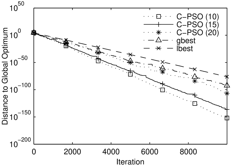
Figure 4.7: Sphere–closeness to global optimum for C-PSO(10, 15, 20), gbest, and lbest

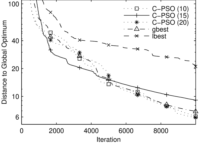
Figure 4.8: Rosenbrock–closeness to global optimum for C-PSO(10, 15, 20), gbest, and lbest

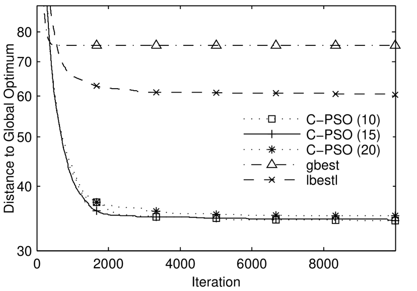
Figure 4.9: Rastrigin–closeness to global optimum for C-PSO(10, 15, 20), gbest, and lbest

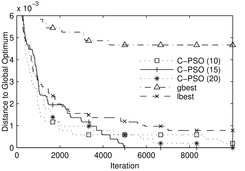
Figure 4.10: Schaffer’s $f_{6}$–closeness to global optimum for C-PSO(10, 15, 20), gbest, and lbest

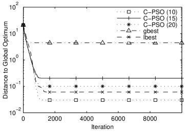
Figure 4.11: Ackley–closeness to global optimum for C-PSO(10, 15, 20), gbest, and lbest

4.5.4 Further Investigation of Optimizers’ Behaviors

The three optimizers, C-PSO (10), lbest and gbest were run on the unimodal Rosenbrock test problem and the multimodal Rastrigin problem. During the simulation run the index of the best performing particle in the swarm was recorded for each iteration. The same parameters used previously for the first criterion were used for this experiment. Figure 4.13 and Figure 4.13 show the best performing particles in C-PSO (10) (top), lbest and gbest (bottom) for the Rosenbrock and Rastrigin problems respectively. For each plot, the index of particles (20 particles) is drawn against the number of iterations elapsed. A dot at (13, 5000) indicates that ‘particle 13’ has the global best value in the swarm during ‘iteration number 5000’.

Figure 4.12: Best particle in the swarm for Rosenbrock problem using C-PSO(10) (top), lbest, and gbest (bottom)

Figure 4.13: Best particle in the swarm for Rastrigin problem using C-PSO(10) (top), lbest, and gbest (bottom)

First, considering Rosenbrock problem shown in Figure 4.13. The status of being the best performing particle in the case of C-PSO is almost uniformly distributed over all particles, once a particle finds a good solution, another particle finds a better one. A reason for this behavior is that once a particle finds the good solution it becomes the best particle in the swarm, making it the best in its neighborhood as well. The particle shrinks its membership level one by one and reduces its influence on other particles accordingly. Neighbors of this superior particle will carry its influence to other clubs they are member of, so other particles are still indirectly guided by it, but are more free to find a steeper way down the hill to the global optimum. Once a particle finds it, it becomes the new best particle and continues or starts shrinking its membership level (because it may become the best in its neighborhood before becoming the global best). The particles which are no longer the best in their neighborhood regain their default membership level to increase their chance in learning from better particles to become the new global best, and the cycle continues.

On the other hand, the best particle status in lbest goes bouncing between two particles on the ring (note that particle 1 is connected to particle 20) as shown in Figure 4.13 (middle). The particles outside this arc search totally inefficient regions of the search space. This is clear from the fact that none of them shows up even once as the best particle in the swarm for the last 7500 iterations. This clustering mechanism may help the algorithm to overcome local optima in multimodal problems, but in unimodal problems it has detrimental effect. The reason that gbest algorithm came second to C-PSO in both unimodal problems is clear in Figure 4.13 (bottom). After around 2600 iterations, 12 particles acted as guides for the other 8 particles and literally dragged them behind. None of the 8 particles showed superior performance till the end of the 10000 iterations.

Second, considering the Rastrigin problem presented in Figure 4.13, this multimodal problem requires diversity in the swarm and a clever social network to overcome local optima. The property of fully connected social network in gbest provokes all the particles to jump to the best found position by all particles in the swarm. This makes the first 1500 iterations for gbest look almost the same for both unimodal and multimodal problems. But after these 1500 iterations the algorithm prematurely converges in the case of the multimodal Rastrigin problem as shown in Figure 4.13 (bottom). On the other hand, lbest algorithm presented in Figure 4.13 (middle) maintains its diversity for a longer period than gbest does. Along with its clustering property explained earlier, it manages to escape local optima to some extent and get closer to global optimum than gbest can get.

Finally for the C-PSO optimizer as shown in Figure 4.13 (top), the algorithm maintains diversity longer than gbest and lbest do. Moreover, the best performing particle status is distributed over the particles, unlike lbest, and the particles do not jump over the best particle once it emerges. This can be seen as the particles create more clusters than in the case of lbest and gbest. These clusters represent local optima found by the particles. The most interesting result found is the ability of the C-PSO to explore new regions after a period of stagnation.

As can be seen C-PSO finds better regions at around iteration 5200 after it has stagnated for nearly 2000 iterations. An explanation for this behavior is that the best performing particles in their neighborhood create different points of attraction for the particles. The particles are grouped according to their clubs’ membership and search the space around these points of attraction. At the same time, the worst particles on their neighborhood expand their membership and bridge the influence between different groups of searching particles. If a searching group finds a better solution, its influence is transmitted over the bridge acting particles to other groups and diverts them from searching inefficient regions indefinitely. They start searching for other optima which could be better than the best one found and create different points of attraction, and the cycle goes on.

4.5.5 Convergence Speed

The second criterion to be considered is the convergence speed of the algorithms. As explained earlier, it is being measured by the number of iterations the algorithm takes to reach a certain degree of closeness to the global optimum. This number of iterations should be small enough to reflect the ability of the algorithm to converge rapidly, and not its ability to escape local optima and achieve better values at later stages of the run. On the other hand, the closeness value chosen should lie close enough to the global optimum to be efficient in practical applications. The closeness values for the five benchmark problems that are satisfied by most algorithms are chosen to be around the range of [500, 1000] iterations. These closeness values are shown in Table 4.4 next to problem names.

Table 4.4: Number of iterations needed to reach a certain degree of closeness to global optima for the five optimizers. (best values are bold faced)

Algorithm	Avg.	Med.	Max.	Min.	Suc.%
	Sphere–(closeness = 0.0001)
lbest	1030.8	1036	1103	965	100
gbest	684.88	672	1012	489	100
C-PSO (20)	611.68	571	1057	421	100
C-PSO (15)	528.18	506.5	711	417	100
C-PSO (10)	518.14	513.5	652	443	100
	Rosenbrock–(closeness = 100)
lbest	1429.6	907	7465	604	98
gbest	874.3	425	6749	251	100
C-PSO (20)	697.3	424	4537	240	100
C-PSO (15)	569	473	1605	218	98
C-PSO (10)	725.8	376	6016	226	98
	Rastrigin–(closeness = 50)
lbest	1695.7	1068	8015	500	26
gbest	250	221	313	216	6
C-PSO (20)	813.9	702	3396	254	88
C-PSO (15)	695.4	597.5	1829	262	88
C-PSO (10)	753.3	667	1932	299	96
	Schaffer’s $f_{6}$–(closeness = 0.001)
lbest	1076.2	422	7021	84	92
gbest	791.1	279.5	4276	60	52
C-PSO (20)	1138.3	524	8462	80	100
C-PSO (15)	1120.1	432	4966	88	100
C-PSO (10)	945.6	401	9668	48	98
	Ackley–(closeness = 0.01)
lbest	968.2	954.5	1531	827	96
gbesta	499	499	499	499	2
C-PSO (20)	831.1	806	1148	610	92
C-PSO (15)	800.6	793.5	1141	570	84
C-PSO (10)	863.7	841	1151	672	98

The figures presented in Table 4.4 are compiled from the same results data set collected for the first criterion. They represent the Average, Median, Maximum, Minimum and Success rate of 50 independent simulation runs for the five optimizers. Only data of successful runs were used to evaluate these values, so the sample number is not the same for all figures.

It can be seen from Table 4.4 that C-PSO (15) achieves the overall best results. For the Sphere problem, all the algorithms achieve the desired closeness in every single run, although C-PSO (10, 15) come ahead of them. The situation is similar in the second unimodal Rosenbrock problem, however, the success rate is lower for lbest and C-PSO (10, 15).

Moving to multimodal problems, gbest shows poor performance in reaching the closeness values. For Rastrigin and Ackley problems, it only succeeds in six and two percent of the runs respectively, compared to much higher success rates in all C-PSO versions. C-PSO (15) outperform all the other algorithms for Rastrigin and Ackley problems, except for the Rastrigin problem where it comes second to C-PSO (20) regarding the minimum number of iterations in the 50 samples. gbest were not considered in the comparison for Rastrigin and Ackley problems due to its very low success rate. Finally for Shaffer’s $f_{6}$ problem, gbest achieved the best results for the mean, median and maximum number of iterations. It should be noted however that it has a low success rate of 52% which is almost half the success rate for all C-PSO versions. This low success rate makes it unreliable in practical applications.

4.6 Comparison to EAs

The PSO algorithm was compared to EAs once it was developed [88]. Kennedy and Eberhart described it as an algorithm that stands somewhere between GAs and EP; the adjustment towards local and global best positions exploits the accumulated knowledge by the swarm, analogously the crossover operator recombines parts of good parents hopefully to produce good offspring. While PSO resembles EP in its reliance on stochastic processes ($rand_{1}$, $rand_{2}$). Some people argue that PSO is indeed an EA, but Kennedy and Eberhart do not share this opinion [92]. However, it is unquestionable that both of them are nature inspired—population-based algorithms, they do operate a population of complete solutions; at any moment during the run, the algorithm could be stopped and $N$ solutions to the problem will be available, where $N$ is the population size.

GAs employ the concepts of evolution and Darwinian selection, while PSO is powered by social interactions. In GAs, the worst individuals perish and get replaced by more fit ones, while in PSO the worst particles do learn from their neighbors, however subsequent positions of the swarm may be perceived as different GA generations; at the end of each iteration of a PSO algorithm, the old particles are killed and replaced by their offspring at the next positions. But this analogy entails many assumptions, such as assuming that every particle must produce one, and only one offspring, and this offspring will replace its parent.

The social interaction among swarm members brings them closer to each other, the particles tend to pursue their superior neighbors and thus converge to a point in one of the promising regions they discovered. On the other hand, highly fit individuals tend to produce more offspring than less fit individuals in the population of a GA algorithm, leading to convergence to a point in one of the best found regions. PSO particles do learn, while GA individuals do evolve.

The crossover operator of a GA resembles the social interactions of PSO particles. When two individuals are recombined, the produced offspring stands somewhere between the parents, while social interaction between two particles at two points in space brings one of them to an intermediate point.

The mutation operator of a GA has its counterpart as well. The stochastic variables $rand_{1}$, and $rand_{2}$ are their image in PSO. The mutation operator ensures that the probability of sampling ever point in the solution space is never zero. It kicks an individual to a point that other deterministic operators may never take it to. Similarly, the stochastic variables in PSO drives the particles to regions that may seem poor when evaluated by their personal and neighbors experience measures.

GAs was proposed in 1960s while PSO was developed in 1995. Due to this gap in time, GAs have been experimented and developed more rigorously than PSO. GAs are applied in many real-world applications ranging from control engineering, water treatment, and job scheduling, to image processing, and military tactics. PSO on the other hand has been applied less extensively to real-world applications due to its young age and scant mathematical analysis. The stability, reliability, and availability of both algorithms are not verified so far by closed form mathematics, thus their use is not advisable in critical applications where its failure may result in injury or expensive repair.

Despite many empirical studies and comparisons between PSO on one hand and EAs or GAs on the other hand, no definite conclusion was shared among these different studies. Some of them suggested the use of PSO in some practical problems [117], while others were less enthusiastic about it [118]. This different conclusions may further assert the NFL theory, which states that [14]:

“…all algorithms that search for an extremum of a cost function perform exactly the same, when averaged over all possible cost functions”

Chapter 5 Applications in Control Engineering

It was the feats accomplished by evolution, natural selection and social interactions that inspired researchers to mimic these natural mechanisms as computer paradigms to solve numerous problems. These optimizers were already in the works long time ago, and their obvious successful results is the strongest proof of their applicability in real-world problems. But reverse engineering nature resulted in a new situation. In an ordinary situation, an engineer who is faced with a problem works-out a mathematical analysis of the problem and proceeds step by step, in a logical fashion, to create a problem solver. The applicability and efficiency of this solver are tested and verified by practical application over a period of time. On the other hand, the efficiency and applicability of a solver employed by nature has already been tested and verified through millennia. Researchers extracted the solver out of the system and applied it to different problems. Today, many researchers and scientists work out mathematical analysis to find out why these solvers work, and develop a closed-form mathematical explanation and proof for them.

No wonder why a generic problem solver such as GAs would be applied to complex problems which proved to be unyielding to the rigid, conventional, analytical, problem solvers, such as control engineering problems. In fact, the application of GAs in control engineering was proposed concurrently with the algorithm itself when John Holland presented them in his PhD thesis titled “Adaptation in Natural and Artificial Systems: An Introductory Analysis with Applications to Biology, Control, and Artificial Intelligence” back in 1975 [39]. Although PSO is still in its infancy, the increasing number of publications proposing and reporting encouraging results of its application in control engineering problems indicates its applicability and efficiency in such problems [119, 120, 121, 122, 123].

5.1 Why Computational Intelligence?

The major power of CI techniques stem from their generic nature, which tolerates lack of information about the system in study, can handle a problem with mixed type of variables, welcomes ill-shaped system landscapes, provide flexible way in representing decision vectors, can efficiently handle constraints by different ways, and are not subject to many of the limitations that traditional optimizers are subject to. All these merits directly address many of the difficulties found in control engineering problems.

If it is hard to create a mathematical model for the control system under study due to lack of information about it, its high non-linearity, or its stochastic nature, then conventional techniques, which are problem specific, will not produce satisfactory results. On the other hand, CI methods, which are generic, can deal with this lack of information and uncertainty, and any acquired information about the system can be utilized by the algorithm and incorporated in the model on-the-fly.

Yet another benefit of the generic nature of CI techniques is their ability to handle problems with mixed types and units of variables. Since the algorithm works on encoded variables, it can handle solution vectors such as ($\text{H}_{2}\text{O}$, $2\pi\,^{\prime\prime}$, $-4\,^{\circ}\text{C}$, Italy, $\frac{5.6}{7}$Kg) with no problem. However, this is not an easy task for a conventional method indeed.

Traditional optimization techniques perform badly on problems with ill-shaped landscapes. Multimodality, non-differentiability, discontinuity, time-variance, and noise may render a traditional method inefficient, or may even block its application. However, these properties are not a source of difficulty for CI methods [1].

Any convenient representation of solutions can be used with a CI method. However, the adopted representation can dramatically affect the performance of the algorithm used, and henceforth, the quality of solutions obtained [124]. One representation may encode decision vectors in such a way that help exploring the solution space more effectively than another representation, while a third one could be computationally less expensive and runs faster than a fourth one. Moreover, the representation itself may evolve over time, so the algorithm would eventually produce the most efficient representation which encodes optimum solutions. This evolving representation is depicted in GP models [53]. A good representation should come with suitable variation operators, or else it will not be possible to generate new solutions from the old ones, or produce mostly infeasible or inferior solutions which require extra computational cost to repair them, which may lead to random search or even worse. The flexibility in representation offered by CI optimizers may be seen as a sort of shortcoming or advantage.

Almost all control and engineering problems in general are constrained problems. These constraints can be soft constraints, such as the riding comfort of an elevator, or hard constraints, such as the stability of the elevator and the limit of its actuators. Dealing with these constraints, specially in discontinuous problems poses quite a challenge for traditional optimizers. But for CI techniques, these constraints can be handled easily in different ways. These constraints may be embedded in the representation scheme used, so evolving the encoded parameters always yields a valid solution. Another way of dealing with constraints is penalizing unfeasible solutions, different penalty strategies can be used considering the degree of constraint violation and the number and type of constraints violated and so forth. Alternatively, the constraints can be imbedded into the problem as new objectives and then by solving the new problem as a non-constrained problem, feasible solutions to the original problem are obtained [125].

CI methods are not subject to many of the limitations and constraints that traditional methods must adhere to. For example, the evaluation of the discrepancy between the expected output of a controlled system and the obtained one, which is known as the error, is done in many traditional techniques by using the Root-Mean-Square (RMS) of the error. However this evaluation technique is biased. As shown in (5.1), RMS underestimates errors below 1 and over estimates errors above 1 [126]. This bias does not exist in the Sum of Absolute Error (SAE) evaluation as shown in (5.2). However, only the former is applicable in traditional methods due to the discontinuity of the absolute function used in the later. CI techniques, on the other hand, have no problem in utilizing any one of them.

RMS $$\Rightarrow\quad (0.9-0.6)^{2} =0.09\qquad (3-(-5))^{2} = 4$$ (5.1)

SAE $$\Rightarrow\quad |0.9-0.6| =0.3\qquad |3-(-5)| = 2$$ (5.2)

5.2 When to opt out?

Despite many benefits obtained by using CI techniques in control engineering applications, in some situations it is not advisable to use them.

If the system under study is simple, well-known, with low degree of randomness and tolerable amount of noise, and can be approximated by a linear system with a low degree of error if it is not a linear system in the first place, then traditional techniques providing analytical solution may be the method of choice, and it is unlikely that CI techniques will outperform it. The flexibility offered by the Swiss-knife with its various tools does not make its tiny scissors a powerful tool in cutting material when compared to conventional scissors that can only handle this task [15].

CI methods are known to be computationally intensive. The algorithm that operates a population of agents working (at least virtually) in parallel and evaluates their fitness every iterations then classifies or orders them according to their fitness is indeed resource intensive, both in memory, and computational power. This resource intensive property of CI techniques present two handicaps. First, it is expensive (money perspective), which adds extra cost to the control system and reduces its price competitiveness when compared to other control systems using traditional techniques which are less computationally intensive. Second, the computational power needed to run some CI optimizers may not be available, or could be hard to fit in the control system, which may lead to slow and unsatisfactory performance.

Although EAs and SI methods have been applied in many practical applications, and some engineering consultancy firms are specialized in providing CI solutions for various engineering problems. These methods are not guaranteed to succeed. Their convergence and stability have not yet been proved using closed loop mathematical analysis, albeit few mathematical proofs [39, 110] that relied on many assumptions to facilitate the analysis, and proved the convergence of a simple model which is quite different from the practical models being used today. It is common in CI literature to verify the effectiveness of an optimizer by repeatedly running it on a benchmark problem over 50 times to withdraw the possibility of chance in the solutions obtained. This scepticism is far more less in the application of traditional techniques. Due to lack of mathematical analysis and presence of stochastic variables in CI techniques, they are not welcome in many critical applications where any failure may result in injuries or leads to expensive repair.

Traditional techniques are used in many on-line applications today, however the use of CI methods in this venue presents quite a challenge. In on-line applications, the system must decide on the action at every time step, which requires reaching a good decision during this time frame, but as pointed out earlier CI methods are computationally intensive, and henceforth, the time it takes to converge or reach a good decision may exceed the limited time frame which is obviously not acceptable. Moreover if the best individual in the population is chosen at each time step even if convergence was not achieved, the system will perform poorly and unsatisfactory results will be obtained, or even worse, the system may go unstable.

Another major of concern when using CI methods for on-line applications is the nature of these optimizers themselves. These techniques work by learning from their past performance and mistakes. So if they utilized the process which they operate directly, sever consequences may result. For example, it is known that most CI techniques provide poor solutions early in the run, then the quality of these solutions improve as the algorithm is fed-back with their results. However, it is not acceptable in most applications to waste materials, cause damage to equipments, or reach unstability for the sake of teaching the algorithm. To overcome this undesirable behavior, a traditional method may exist in the system as a control scheme backup and whenever the decision of the CI technique goes beyond a predefined threshold, the traditional backup optimizer is activated, and the CI one steps aside. However restricting the operation of a CI optimizer in such a way prevents it from learning and improving its performance, so even after long running time, its performance may still be unsatisfactory.

Another possible use of CI techniques is to use them in optimizing the parameters of a controller on-line. In this situation, the optimizer gets its feedback from the process itself and a model of the process is not required. After the parameters have been properly tuned, they get fixed on these values and the controller is put in real on-line operation.

However, in some situations it becomes extremely hard to evaluate any of the population individuals using the real system. For example, it is not possible to stop an electricity power plant generating power for millions and operate it under varying conditions for the sake of system identification. In such a situation, the algorithm may watch and learn from the normal input-output data of the operating system. However, as with the case of the backup system presented earlier, the algorithm will not be able to develop a good understanding of the model because its knowledge was confined to a small range of the ordinary input-output data generated under normal conditions.

5.3 Applications

CI techniques have been used in numerous applications, they vary from controller design and system identification, to robust stability analysis, fault diagnosis and robot path planning [1, 127]. They can be used as a direct or indirect design tool.

5.3.1 Controller Design

A CI optimizer can be used in tuning controller parameters, designing its structure, or doing them both. It can be used as the only design tool, or assisted with other techniques in a hybrid design system. Depending on the application of the controller, the fitness function will be defined accordingly. In a dairy processing factory, it will be desirable to abruptly change the milk temperature for the pasteurization process. In such a case, the fitness function will be inversely proportional to the rise time of the milk temperature while its overshoot will be less significant. On other applications involving passenger’s comfort, the overshoot of the vehicle’s speed should be emphasized in the fitness function used.

Parameter Tuning

For the parameter tuning problem, the algorithm operates a population of individuals where each one of them encodes a set of controller parameters. The fitness of each individual is determined either by a the controller itself or by a model of it. If the representation used allows infeasible solutions, such as those leading to system instability, they are penalized according the penalty system used. Depending on the efficiency of the algorithm used, the optimizer may eventually discover a good set of controller parameters.

Many researchers used GAs and PSO to tune Proportional-Integral-Derivative (PID) controller parameters. Among these efforts, Herrero et al. [128] used a GA to tune an optimal PID controller for a nonlinear process model in various situaltions: model errors, noisy input, IAE minimization, and following a reference models. They concluded by recommending its use for off-line parameter tuning due to high computational cost required by the optimizer. The same problem was tackled in [129] but using a PSO algorithm with some modifications. The modified PSO optimizer achieved encouraging results by achieving lower settling time over various transfer functions when compared to the performance of a PID controller tuned using the traditional Ziegler-Nichols method.

Alternatively, CI optimizers may be used to tune the parameters of a controller indirectly. In this case, they are used to tune the parameter values of a design technique, which in turn, tunes the controller parameters. For example, a GA may be used to tune the Linear Quadratic Gaussian (LQG) method parameters, or tune the pre- and post-plant weighting functions for the $\mathcal{H}_{\infty}$ method, then any one of them can be used to tune the controller parameters. Using this procedure, the stability of the system will be guaranteed by the LQG and $\mathcal{H}_{\infty}$ methods, while a GA will be used to find their best parameters [1].

Structure Design

The power of CI techniques is unleashed when utilized in the structure design of a controller. Unlike parameter tuning where there are traditional straightforward, well known and trusted optimization techniques, the controller structure design requires human experience in the field. Henceforth, developing a CI method that can manipulate and develop a good controller structure would provide a faster and probably cheaper alternative for the human based design.

GP has an advantage over many other CI techniques when applied to the automated design of controller structure because the structure of GP individuals evolve concurrently with the value of the genes. So, it will be straightforward to encode each individual as a variable length sequence of parallel and series building blocks of control elements. The GP optimizer will evolve these individuals using a library of those control elements building blocks provided by the user to find the best structure and parameters for this structure using the limited set of elements.

Koza et al. used GP for automatically synthesizing the design of a robust controller for a plant with a second-order lag [130]. They reported better for the GP method when compared to a PID compensator preceded by a low-pass pre-filter regarding the integral time-weighted absolute error, rise time, and disturbance suppression.

5.3.2 Fault Diagnosis

Another application of CI methods is system fault diagnosis where these algorithms can be used to detect the presence of a fault, isolate it, and identify or classify the fault [1].

Miller et al. used GAs to spot the fault in a system [131]. Given the probabilities that a particular disorder causes a particular symptom, the algorithm was able to spot the fault from a collection of faults given the set of symptoms that indicate that a problem exists.

In an effort to increase the reliability of the system, Coit and Smith used a GA to find the best system configuration by selecting components and levels of redundancy to collectively meet reliability and weight constraints at a minimum cost [132].

5.3.3 Robust Stability Analysis

Fadali et al. used a GA in a stability analysis context [133]. They reduced the stability robustness analysis for linear, time-invariant, discrete-time system to a problem of searching for the roots of the system’s characteristic polynomial outside the unit circle. Since the presence of such a point that lies outside the unit circle is a sufficient condition for system instability, a GA searching for such a point will classify the system as unstable if that point is found. However, if the point was not found the stability of the system is not guaranteed.

The GA robust stability analysis is a strong contender when compared to the traditional analysis techniques which rely on simple uncertainty structures, or other techniques with more complex structures but are infeasible to implement.

5.3.4 Robot Path Planning

Yet another field that CI techniques has successfully applied to is robot path planning. The path planning problem is an optimization problem that involves computing collision free path between two locations. Beside this goal there are other criteria of minimizing the travel distance, time, energy, safety, and smoothness of the path. The collection of all this criteria in a dynamic system where many robots may work concurrently on the same object makes conventional approaches such as cell decomposition, road map, and potential field impractical to apply.

Elshamali et al. used a GA with a floating point variable length chromosome representation to tackle this problem [134]. Each chromosome represents a path as a sequence of nodes, the first one is the starting point and the final one is the final destination. The variable length chromosome allows a flexibility of path creation. They used a weighted combination of the path distance, smoothness, and clearance as the fitness function. They used five operators to evolve the population with different probabilities, and used a strategy to ensure population diversity. This algorithm was effective and efficient in solving different types of tasks in dynamic environments.

5.4 System Identification

Understanding why a system behaves in a certain way and predicting its future behavior is a major field of research in control engineering. The system in question could be any thing from bacteria growth and stock markets to global warming and galaxy movements. Although some of these systems, such as the stock market, is a man-made system, its exact behavior cannot be determined given current and past inputs to this system. This uncertainty in such systems is due, in large part, to the complexity of the system in question. In other situations, some simple man-made systems deviate from its designed behavior due to aging, wearing out, or change in a system parameter that was assumed to be static. For example, the performance of car brakes changes over time. The behavior of natural systems such as galaxy movements and global warming is far more complex and is much more harder to understand.

System identification involves creating a model for the system in question that, given the same input as the original system, the model will produce an output that matches the original system output to a certain degree of accuracy. The input or excitation to the system and model, and their corresponding output are used to create and tune that model until a satisfactory degree of model accuracy is reached. As shown in Figure 5.1, the input $u(t)$ is fed to both the system and the model $M(\hat{\theta})$, then their corresponding outputs $y(t)$ and $\hat{y}(t,\hat{\theta})$ are produced and matched. The error $e(t)$ reflects how much the model matches the system; the lower the error, the more the model resembles the system.

System identification of practical systems is not an easy task to be accomplished by traditional techniques [135]. Most real-world systems contain dynamic components. Due to this dynamic nature of the system, the output of the system does not only depend on the current input to the system, it depends on the past inputs and outputs to and from the system. As the number of old data affecting the system (maximum lag) increases, the number of terms used in the classic system models increases substantially. Another difficulty encountered in identifying real-world system is its nonlinearity. In order to simplify the problem, many engineers represent the non-linear system by a linear model, however the performance of this simplified model will not be satisfactory in mission critical applications. Although there are some classic models that can represent non-linear models, such as the Non-linear Auto-Regressive Moving Average model with eXogenous inputs (NARMAX) model, the number of these model terms explodes as the degree of nonlinearity increases. The number of terms in a NARMAX models for a modest real-world system with a nonlinearity order of 3 and a maximum lag of 6 will have $\binom{15}{3}=455$ terms. Obviously, the complexity of such a system and the huge volume of data required to calculate the least-square estimates would render this model impractical [127].

System identification is essential for many fields of study that extend beyond control engineering. It is desirable to identify the the global warming system in order to understand its mechanism and try to slow it down or reverse it. It is crucial for an astronomer who tries to understand the planetary movements and correlates it with various astronomical phenomena. Creating models for human organs helps physicians and medical engineers to create a substitute for these organs. While understanding an industrial process helps an engineer to control, maintain it, and diagnose its faults. The applications of system identification is numerous, but for the sake of brevity it will be approached here from a control engineering perspective, though many of the concepts and procedures involved in the identification process itself are essentially the same for different applications.

Figure 5.1: Process of system identification

5.4.1 Identification Procedure

The system identification process of constructing a system model can be described by the following procedure [135].

1. Data recording: The input-output data of the system are recorded. In some situations, it is possible to conduct an experiment solely for this purpose. In this case, the engineer may have choose when and what input and output data is to be recorded. Furthermore, he may feed the input data of his choice that would maximize the knowledge of the system. In other situations, the engineer can only watch and record few input-output data that the system allows him to monitor under normal operation. It is clear that the data recorded in the later situation would be less informative than the one recorded in the former.

2. Model Set Selection: The next step is to choose a model set that the system under study would be represented by one of its members. This step is not a deterministic one, it is rather subjective. It involves prior knowledge of the system, if available, and the experience of the engineer plays a major here. The system could be modeled by physical laws that reflect the dynamics of the system. A model created by these laws which reflect the physical properties of the system is called a white-box model. However, creating a white box model for real-world (complex) systems is a challenging task. As a compromise to the lack of understanding of all physical rules which drive the system, a model that imitates the real system regarding input-output data is sought. A model that merely resembles the system without reflecting a physical soundness is called a black-box model.

3. Model Selection: After the model set is selected, the best model in this set is selected using some of the input-output data recorded previously. In this step, the model parameters are tuned so that the model output would fit the system output as much as possible. The quality of the model is based on a criterion chosen a priori.

4. Model Validation: The next step is to verify the quality of the developed model. The quality assessment is done by comparing the model output to the original system output when both are fed with samples of the input-output data recorded previously (in this case, the validation data are different from the data used for model selection), or with the system in real operation situation (not experimental mode). If the model meets the chosen criteria which reflect the intended use of the model, the model is accepted, otherwise, it is rejected and another model is created. This procedure is repeated until a satisfactory model is created. It is to be noted that a system model will only imitate the original system in certain aspects of interest to the model designer. It will never become a full and true description of the system [135].

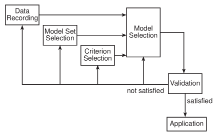
Figure 5.2: Procedure of system identification

The system identification procedure is depicted in Figure 5.2, inspired from [135, pp.9]. The feedback from the ‘Validation’ step to other steps is used to refine or create a new model if the old one did not provide a satisfactory performance. If the poor performance is due to bad selection of criterion that does not reflect the desired system attributes to be imitated by the model, then the feedback to the ‘Criterion Selection’ will be used to modify this criterion or criteria. If deficiency in system matching is due to bad model, then the feedback to ‘Model Selection’ will be used to change the order of the model or tune its parameters. If this modification does not lead to a satisfactory behavior, then the feedback to ‘Model Set Selection’ will be used to select a different model set. The mediocre performance could be attributed to bad input-output data. These data may not be enough informative to be used in model selection and tuning, henceforth, the feedback to the ‘Data Recording’ will be used to create another data set.

5.4.2 Types of System Identification

It is desirable in many control engineering problems to build a model of the system under study. If the system is simple enough (linear, time-invariant, deterministic, single-input single-output system) the model can be built using building blocks representing physical processes (white-box model), and by tuning the parameters of these elements. However, most real-world problems are not that simple. Non-linearity and time-invariance among other properties, make it hard to create an acceptable model of the system using this technique. Henceforth, System Identification can be decomposed into identifying a structure for the system, and identifying the parameters of a structure.

Parameter Identification

Because it is hard to create a white-box model for complex systems, some parameterized models that can describe a system to some degree of accuracy can be used instead (grey-box model). These models, such as the ARX model and its variants, offer a reasonable degree of flexibility so that if the model is well-tuned, the model output will match the output of the real system to a high degree. The process of identifying the values of these parameters are known as parameter identification.

CI techniques can be used to tune the values of the parameterized models in a similar way to that used in parameter tuning of a controller presented earlier. The CI algorithm operates a population of potential solutions to the problem. The individuals of this population encode different solutions to the problem, and as the algorithm proceeds, it tries to find better solutions according to some quality measure, which is typically the difference between the predicted output of the system based on the created model, and the measured output of the system (prediction error). Depending on the efficiency of the algorithm used, it may find a good set of parameters that produces a tolerable prediction error. Following this approach, Voss and Feng used PSO to find the parameter set of the Auto-Regressive Moving Average (ARMA) parameterized model [136]. They reported superior results of the PSO-based parameter tuning when compared to the International Mathematical Libraries routines using noisy (real-world) data.

Structure Identification

In some problems the accuracy provided by parameterized models is not satisfactory. This situation is encountered in complex systems where the limited flexibility of the parameterized model does not yield a tolerable error. Moreover, the choice of the parameterized model to be used depends mainly on the experience of the designer and is a matter of personal judgement.

The limited flexibility of the parameterized models and lack of an objective method for selecting such a model makes CI methods a strong contender. CI based techniques such as GP offer high degree of flexibility. From a limited set of elements, the algorithm can develop and evolve different models of different complexities that can resemble the real system to a high degree (black-box models).

Gary et al. used GP to identify parts of the nonlinear differential equations and their parameters describing a model of fluid flow through pipes in a coupled water tank system [137]. The model created using this technique gave an accurate representation of the real system.

5.4.3 Identification Models

As mentioned in the previous section, the selection of the model set to be used in identification is one of the most important steps in the system identification process, and probably the hardest one. The selection decision does not follow a straightforward path and is subject to experience and faith in previously tested and well-known models. These models may include, but not limited to, the following model sets:

Functional Models

One of the first non-linear system representations was the Volterra series representation developed by the Spanish mathematician Vito Volterra. Analogous to Taylor series, it provides an expansion of a dynamic, non-linear, time-invariant system. It describes the system output as the sum of the 1${}^{\text{st}}$ order, 2${}^{\text{nd}}$ order, 3${}^{\text{rd}}$ order …etc. operators, and every operator is described with a transfer function called a Volterra kernel. Due to its general use, it is sometimes referred to as a non-parametric model. A non-linear system can be described by the following Volterra series:

$$y(t)=\sum_{n=1}^{\infty}\int_{-\infty}^{\infty}d\tau_{1}\dotsm\int_{-\infty}^{\infty}g_{n}(\tau_{1},\dotsm,\tau_{n})\prod_{r=1}^{n}u(t-\tau_{r})d\tau_{n}$$ (5.3)

where $u(t)$ and $y(t)$ are the system input and output respectively, $g_{n}$ are the Volterra kernels of the system, and $\tau_{i}$ are time variables.

Volterra series representation may not be the choice for practical non-linear systems for two reasons. First, the difficulty encountered in practical measurement of Volterra kernels detracts from the applicability of the technique. Second, the number of terms required to represent a non-linear system explodes with the degree of nonlinearity.

Artificial Neural Network Models

ANNs are a strong contender to other black-box models. With their parallelism, adaptability, robustness, they can deal efficiently with non-linear models, and with their repetitive structure, they are resilient to failures, since any node can play any other node’s role by adjusting its weights [138]. The Radial Basis Function (RBF) and the Multi-Layered Perceptron (MLP) networks are among the most widely used ANN schemes in system identification.

RBF networks consist of an input layer, one hidden layer with RBF activation function, and a linear output layer. The most popular RBF activation function takes the gaussian form:

$$\varphi_{i}(\text{\bf x})=\exp\left(\frac{-\|\text{\bf x}-\text{\bf c}_{i}\|^{2}}{\sigma_{i}}\right)$$ (5.4)

where $\varphi_{i}$ is the activation function excited by an input pattern x, $\text{\bf c}_{i}$ is a vector defining the center of the RBF $\varphi_{i}$, and $\sigma_{i}$ is a scaling factor for node $i$.

After the input pattern is fed through the input layer, a hidden node only responds to a pattern x within a certain distance (Euclidian sense) from its center $\text{\bf c}_{i}$. The excitation values of the hidden nodes are then passed to the output layer. The weighted sums of these values are produced by the output layer to make the model output according to the following rule:

$$h_{j}(\text{\bf x})=\sum_{i=1}^{m}w_{ij}\;\varphi_{i}(\text{\bf x})$$ (5.5)

where $h_{j}$ is the output produced at the output node $j$, $w_{ij}$ is the weight between the hidden node $i$ and output node $j$.

The identification process involves tuning the weights $w_{ij}$, the centers $\text{\bf c}_{i}$, and the scaling factors $\sigma_{i}$, where $i=(1,\dotsc,m)$, and $j=(1,\dotsc,n)$, so that the model outputs $h_{j}(\text{\bf x})$ would match the real system outputs $y_{j}(\text{\bf x})$.

Training the network to optimize $c_{i}$ and $\sigma_{i}$ is done using an unsupervised technique, such as the Hebbian and competitive learning rules, while the optimization of the weights $w_{ij}$ is done by a supervised method such as the following rules:

$$w_{ij}^{t+1}=w_{ij}^{t}+\Delta w_{ij}$$ (5.6)

$$\Delta w_{ij}=\eta\;(y_{j}(\text{\bf x})-h_{j}(\text{\bf x}))\;\varphi_{i}(\text{\bf x})$$ (5.7)

where $w_{ij}^{t+1}$ is the new synaptic weight value, and $\eta$ is the learning rate.

Alternatively, MLP networks may be used instead of RBF. In this case, the network may contain more than one hidden layer and the activation function may take other forms such as the logistic or sigmoidal function.

RBF networks are known to be local learning networks because they can develop a good understanding of region when given few learning data sets in that region, however, they cannot generalize. Henceforth, they are suitable when few data sets are available, and only the neighborhood of these sets is of interest (interpolation applications). On the other hand, MLP networks are global learning networks. They do a better job in generalization, but they need a high number of data sets to learn (extrapolation applications).

ANNs are prone to over-fitting, they may even fit to the noise accompanying the input leading to prediction far from the training set data. Even in the absence of noise, MLP may suffer over-fitting and produce wild predictions.

Among its applications in system identification, ANN was used for lung cancer cell identification [139], aerodynamic identification [140], sensor data fusion modeling [141], and micromachined accelerometers identification [142].

Fuzzy Modeling

Fuzzy sets and fuzzy logic are used to incorporate experts’ knowledge in control and industrial applications. By reversing this process, the data acquired from a system can be used to develop a knowledge of this system and identify it.

The available knowledge of the system to be identified may come from two sources: An input-output data set, or an expert knowledge of the system. Generally, there are two main approaches for system identification based on fuzzy logic by using those two sources of information [143]:

In the first approach, the qualitative expert knowledge is transformed into a set of if-then rules to build a model structure. Then the parameters of this structure, such as the membership functions, are tuned using the input-output data set. Since a fuzzy model can be seen as a layered structure, similar to ANN, standard learning algorithms can be applied to it as well.

In the second approach, the data are used to construct the structure the model in the absence of expert knowledge initially. Later, if such knowledge came through, they can be used to modify the rules or create new ones.

Fuzzy modeling is appropriate for interpreting human knowledge about the system which may be expressed in natural linguistic rules and non-crisp sets. Moreover, this kind of modeling can process imprecise data and deal with uncertainty. It provides a transparent representation of the system based on a number of if-then rules which are similar to human reasoning and can provide an intuitive understanding of the system. On the other hand, fuzzy modeling suffers from the curse of dimensionality.

The Evolutionary Approach

EA and SI algorithms are strong contender to the previously mentioned techniques employed in system identification. Unlike these techniques EA can be used in structure identification (black-box models), or in parameter identification (white-box models) due to their robustness and flexibility explained earlier in Chapter 3 and 4.

In parameter identification, the algorithm tunes the parameters of the model until the output of the model matches the output of the real system to a desired degree of accuracy. For example, in identifying the values of different resistors and capacitors in an electric motor, a model for this motor is created and the values of these components are tuned by the algorithm until the output produced by the model for a certain input matches the output of the real motor fed with the same input.

In structure identification, instead of tuning the parameters of the model, the algorithm modifies the structure of the model. This can be achieved by selecting the terms of the Volterra series used to model the system or by modifying the structure of the ANN by selecting the number of layers and nodes in each layer.

5.5 Identification of an Induction Motor

Induction motors are the most widely used motors in industry because they are simple to build and rugged, reliable and have good self-starting capability. Due to their wide spread in industry, it is of great importance to devise a technique that can estimate different parameters of these motors which can’t be measured directly for different reasons. In this section, a model for the induction motor will be created, then different EA, SI, and a traditional technique will be explained before being used to identify six parameters of the motor. The results obtained using these optimizers will be presented and analyzed in detail and a conclusion will be reached.

5.5.1 Induction Motor Model

In this induction motor model, which is based on the model presented in [144], the three-phase voltages and currents are transformed to complex notation for simplicity, and the model is then treated as a two phase system. After the differential equations of the system are solved, the three-phase currents are evaluated and compared to their counterpart in the real system. The absolute value of the difference between the estimated and measured currents over a certain period of time indicates how well the model resembles the real system, and henceforth, how well the estimated parameters match their real counterparts. To create such a model, first, the three-phase input voltages to the motor, $u_{1}$, $u_{2}$, and $u_{3}$, are transformed to complex notation. The voltages applied to the stator windings take the form:

$$u_{s} =u_{sd}+ju_{sq}$$ (5.8)

$$u_{sd} =\frac{1}{3}(2u_{1}-u_{2}-u_{3})$$ (5.9)

$$u_{sq} =\frac{1}{\sqrt{3}}(u_{2}-u_{3})$$ (5.10)

The rotor voltages are not externally supplied, they are induced from the relative rotation of the rotor with respect to the stator. The equations describing the rate of change of the flux through the stator and the rotor can be described by:

$$\dot{\psi}_{s} =-R_{s}i_{s}+u_{s}$$ (5.11)

$$\dot{\psi}_{r}-j\omega_{r}\psi_{r} =-R_{r}i_{r}$$ (5.12)

Where $\psi_{s}$ and $\psi_{r}$ are the flux through the stator and rotor windings respectively, $R_{s}$, $i_{s}$ are the stator resistance and current respectively, and $R_{r}$ and $i_{r}$ are their counterparts in the rotor, and $\omega_{r}$ is the relative speed of the rotor with respect to the stator.

When the alternating stator voltages are applied to its windings, a magnetic field is produced in the form of a traveling wave. This field induces currents in the rotor windings, which in turn interact with the traveling wave and produce torque which rotates the rotor. This interaction between the stator and the rotor can be seen in the following flux linkage equations:

$$\psi_{s} =L_{sl}\;i_{s}+L_{m}(i_{s}+i_{r})$$ (5.13)

$$\psi_{r} =L_{rl}\;i_{r}+L_{m}(i_{s}+i_{r})$$ (5.14)

Where $L_{sl}$, $L_{rl}$, and $L_{m}$ are the stator, rotor, and mutual inductances, respectively.

By separating $i_{s}$ and $i_{r}$, and applying them in (5.11) and (5.12), the currents will be eliminated from those two differential equations. To solve these equations, $\omega_{r}$ has to be evaluated by:

$$\dot{\omega}=\frac{3}{2JP}\;Im(\psi_{s}^{*}\>i_{s})$$ (5.15)

Where $J$ is the total moment of inertia for the rotor and the load, $P$ is the number of pole pairs, and $\psi_{s}^{*}$ is the conjugate of $\psi_{s}$. For simplification, the counteracting torque of the load and friction were ignored.

By substitution, the following set of differential equations are produced and used to model the system.

$$\dot{\psi}_{sd} =\frac{-R_{s}(L_{rl}+L_{m})}{L_{d}}\;\psi_{sd}+\frac{R_{s}L_{m}}{L_{d}}\;\psi_{rd}+u_{sd}$$ (5.16)

$$\dot{\psi}_{sq} =\frac{-R_{s}(L_{rl}+L_{m})}{L_{d}}\;\psi_{sq}+\frac{R_{s}L_{m}}{L_{d}}\;\psi_{rq}+u_{sq}$$ (5.17)

$$\dot{\psi}_{rd} =\frac{-R_{r}(L_{sl}+L_{m})}{L_{d}}\;\psi_{rd}+\frac{R_{r}L_{m}}{L_{d}}\;\psi_{sd}-\omega_{r}\psi_{rq}$$ (5.18)

$$\dot{\psi}_{rq} =\frac{-R_{r}(L_{sl}+L_{m})}{L_{d}}\;\psi_{rq}+\frac{R_{r}L_{m}}{L_{d}}\;\psi_{sq}+\omega_{r}\psi_{rd}$$ (5.19)

$$\begin{split}\dot{\omega}_{r}&=\frac{3}{2J}\left(\frac{\psi_{sq}(L_{rl}+L_{m})}{L_{d}}-\frac{\psi_{rq}L_{m}}{L_{d}}\right)\;\psi_{sd}\\ &\quad-\frac{3}{2J}\left(\frac{\psi_{sd}(L_{rl}+L_{m})}{L_{d}}-\frac{\psi_{rd}L_{m}}{L_{d}}\right)\;\psi_{sq}\end{split}$$ (5.20)

where

$$L_{d}=L_{sl}L_{rl}+L_{sl}L_{m}+L_{rl}L_{m}$$ (5.21)

Given the input voltage values ($u_{1}$, $u_{2}$, and $u_{3}$), and the estimated motor parameters ($R_{s}$, $R_{r}$, $L_{sl}$, $L_{rl}$, $L_{m}$, and $J$), the state variables ($\psi_{sd}$, $\psi_{sq}$, $\psi_{rd}$, $\psi_{rq}$, and $\omega_{r}$) can be evaluated by solving the differential equations (5.16)–(5.20), and the output, which is the three-phase current values ($i_{1}$, $i_{2}$, and $i_{3}$), can be calculated by:

$$i_{1} =i_{sd}$$ (5.22)

$$i_{2} =-\frac{1}{2}\;i_{sd}+j\frac{\sqrt{3}}{2}\;i_{sq}$$ (5.23)

$$i_{3} =-\frac{1}{2}\;i_{sd}-j\frac{\sqrt{3}}{2}\;i_{sq}$$ (5.24)

5.5.2 Algorithms

Two types of algorithms are used here to carry out parameter identification; Traditional algorithms and CI techniques. The Line Search (LS) method is selected to represent the traditional algorithms, while four other algorithms have been chosen to represent CI techniques. The first one is a GA which falls under the umbrella of EAs, while the other three are PSO variants to represent a second category of CI techniques which is SI methods.

Line Search

The LS method is a simple deterministic local search technique. In this method, the search space is discretized with a unit size of $\delta_{i}$ for the $i^{th}$ dimension. A random point (x) is chosen in the discretized search space and its fitness is evaluated ($f(\text{\bf x})$), and the fitness of its neighboring points are evaluated as well. If the fitness value of most fit neighbor is less than or equals that of x (for a minimization problem), the algorithm moves to this new point and evaluates the fitness of its neighbors. But if the fitness of the most fit neighbor is higher than that of x, the algorithm terminates.

The set of neighbors $\mathcal{N}_{\text{\bf x}}$ for a point $\text{\bf x}=(x_{1},x_{2},\dotsc,x_{n})$ in a $n$-dimensional space contains $2n$ unique points. The position of each point in the set can be determined by moving by a step of $\delta_{i}$ in both directions of the $i^{th}$ dimension; $\mathcal{N}_{\text{\bf x}}=(x_{1}\pm\delta_{1},x_{2},\dotsc,x_{n}),(x_{1},x_{2}\pm\delta_{2},\dotsc,x_{n}),\dotsc,(x_{1},x_{2},\dotsc,x_{n}\pm\delta_{n})$.

This algorithm contains one parameter which is the step size $\delta_{i}$. For the current application, this value was set to 0.1% of the initialization range for the corresponding dimension as explained in Table 5.3.

The algorithm starts by randomly selecting a point in the range shown in Table 5.3. Throughout subsequent iterations, this point is not allowed to fall below the lower limit, but is allowed to take values beyond the upper limit.

Genetic Algorithms

The GA used in this application is based on real value representation as explained in Subsection 3.3.1. The parameters are encoded with real values during initialization to take random values within the bounds given in Table 5.3. The real-valued representation is used to alleviate roundoff errors in decimal-to-binary and binary-to-decimal conversions, and to provide higher degree of accuracy. The Polyploid model was not used here because the cost of storing extra chromosomes and handling them during mating does not worth the marginal benefits outlined in Subsection 3.4.8.

After initialization and fitness evaluation, a tournament selection is used to select individuals for mating. The tournament selection is used to decrease selection pressure and to help maintaining good population diversity. Then a recombination operator is used to create the offspring from the selected parents. In this application, the SBX operator [69] is used due to its strong ability to produce a varied set of offspring which resemble their parents to a certain degree defined by a parameter of this operator ($\eta_{c}$).

After creating the offspring, a mutation operator is applied to the original population, however the most fit individual is immune from mutation. The mutation operator used here is the polynomial mutation [77] because it can produce mutations, similar to those produced in binary GA, with a parameter that defines the severity of mutations ($\eta_{m}$).

The survival selection scheme used here relies on tournament selection to reduce selection pressure and help preserve diversity. However, instead of copying them to the mating pool, the selected individuals were those who make the population of the next generation. An elitism strategy is used here to ensure the survival of the most fit individual to prevent a setback in the best found fitness. The parameters of the GA is presented in Table 5.1.

Table 5.1: GA parameters’ values for the parameter identification problem

Parameter	Description	Value
$N$	Population size	50
$p_{c}$	Crossover rate	0.5
$\eta_{c}$	Crossover distribution index	15
$p_{m}$	Mutation rate	0.01
$\eta_{m}$	Mutation distribution index	15
$ts$	Tournament size	2

Particle Swarm Optimization

Three variants of the PSO algorithm were used here for parameter identification. They are based on the lbest (PSO-l), gbest (PSO-g) topologies, and the C-PSO algorithm.

The particles of the swarm of each one of the three variants are randomly initialized within the initialization ranges of the solution space given in Table 5.3. Initial velocities were randomly initialized as well.

Just as the case with the other algorithms, the particles were not allowed to fly below the lower bounds of the search space but were allowed to take any value above the upper bound. On the other hand, the velocities were not restricted by any bound.

Based on the corresponding topology used in these variants, the particles are affected by different neighbors and update their positions accordingly. The parameters of those PSO variants are given in Table 5.2. It is to be noted here that the inertia weight value for the C-PSO algorithm ($w=1.458$) is twice as much as that for the two other topologies because it is multiplied by a uniformly distributed random number with a mean value of 0.5 leading to an expected value which is the same as those for the two other topologies.

Table 5.2: PSO parameters’ values for the parameter identification problem

Algorithm	Parameter	Description	Value
C-PSO	$N$	Swarm size	20
	$w$	Inertia weight	1.458
	$\chi$	Constriction coefficient	1
	$\varphi_{1}$	Personal learning rate	1.494
	$\varphi_{2}$	Global learning rate	1.494
	$cn$	Number of clubs	100
	$M_{avg}$	Average membership	10
	$M_{min}$	Min membership level	4
	$M_{max}$	Max membership level	33
PSO-l	$N$	Swarm size	20
	$w$	Inertia weight	0.729
	$\chi$	Constriction coefficient	1
	$\varphi_{1}$	Personal learning rate	1.494
	$\varphi_{2}$	Global learning rate	1.494
PSO-g	$N$	Swarm size	20
	$w$	Inertia weight	0.729
	$\chi$	Constriction coefficient	1
	$\varphi_{1}$	Personal learning rate	1.494
	$\varphi_{2}$	Global learning rate	1.494

5.5.3 Experiments

The five previously mentioned algorithms are used to estimate the real parameters of an induction motor which are given in Table 5.3. It is to be noted that the stator and rotor inductances ($L_{sl}$, $L_{rl}$) were combined in a single variable because they are linearly dependent. All the five optimizers used the same fitness function, which evaluates the fitness of the solution passed to it by solving the differential equations based on the parameters of this solution using Matlab’s ode45 solver and accumulates the error which is the difference between the estimated currents ($\hat{i}_{1}$, $\hat{i}_{2}$, and $\hat{i}_{3}$) and the measured currents ($i_{1}$, $i_{2}$, and $i_{3}$). The error value is used as a fitness measure.

$$f(\hat{\theta})=\int_{0}^{T}(|i_{1}-\hat{i}_{1}|+|i_{2}-\hat{i}_{2}|+|i_{3}-\hat{i}_{3}|)dt$$ (5.25)

The error was accumulated at 1000 equally spaced time samples for a one second simulation of the start-up of the motor.

To make a fair comparison between the different optimizers, each one of them were allowed to perform 100,000 function evaluations. So a larger size for the population or the swarm meant lower number of generations or iterations. Since CI techniques are stochastic algorithms, and the starting point of the LS method is randomly chosen, each one of the optimizers were run for 10 times on the same problem and statistical results are produced to decrease the role of chance in the obtained results.

Table 5.3: Real values for motor parameters and their corresponding initialization ranges

	$R_{s}$		$R_{r}$		$L_{sl}+L_{rl}$		$L_{m}$		$J$
Real value	9.	203	6.	61	0.	09718	1.	6816	0.	00077
Min	1.	0	1.	0	0.	002	0.	05	0.	00005
Max	20.	0	20.	0	1.	0	5.	0	0.	001

5.5.4 Results

Figure 5.3 shows the fitness values obtained by the five optimizers through the 100,000 function evaluations of the simulation. The values shown in the figure are the average of the 10 independent runs for each one of the five optimizers. As can be seen, the C-PSO algorithm reached the lowest fitness value among the five optimizers at the end of the 100,000 function evaluations. It managed to reach a fitness value of 0.0019 which is significantly better than a value of 0.1554 for the PSO-l algorithm which came in the second place. Little behind the PSO-l algorithm comes the GA then the PSO-g optimizers, while the LS algorithm lags behind them by a long distance.

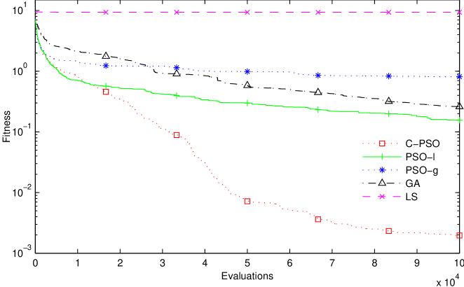
Figure 5.3: Average fitness obtained by the five optimizers against number of fitness function evaluations

From the results obtained in Figure 5.3, the algorithms can be categorized into three groups according to their performance. The first group contains the LS algorithm which totally lacks any capability of escaping local minima. In all the runs, the algorithm was trapped in the first local minima it faced, which happened very early in the run (in the first 5,000 function evaluations in most cases), and subsequent evaluations were unnecessary. In the second group come the PSO-g, GA, and the PSO-l algorithms. The ability of these algorithms to escape local minima is much better than the LS algorithm, which is clear from their much lower final fitness values. Moreover, even at the end of the 100,000 function evaluations, the fitness values of these algorithms were steadily decreasing, however with a small rate. The third group contains the C-PSO algorithm which outperformed all the other optimizers. This algorithm shows much better ability than the two other groups in escaping local minima. Moreover, the rate of fitness decrease for this algorithm is much more higher than that of all the other algorithms, and it even maintained a reasonable decrease rate at the end of the 100,000 function evaluations. These results show how the C-PSO algorithm exploits the available computation power much more better than all the other algorithms.

Regarding convergence speed, it is clear from Figure 5.3 that the C-PSO algorithm is the fastest converging algorithm. By using the number of evaluations needed to reach a value equals 5% of the initial fitness value (roughly equals 10) as convergence speed measure, it can be seen that the C-PSO algorithm was the fastest converging algorithm among all the optimizers. After around 15,000 function evaluations it reached the desired fitness value which the PSO-l algorithm achieved after approximately 23,000 function evaluations. In the third place comes the GA algorithm which needed nearly 60,000 evaluations to reach that fitness value. However, neither the PSO-g nor the LS algorithms achieved the fitness value in question during the 100,000 function evaluations.

The results obtained here confirms the results obtained in a similar parameter identification study presented in [144], as the PSO algorithms (on average) achieved lower final fitness values and higher convergence speed, which was the case here as well.

Further statistical analysis of the results is shown in Table 5.4. As can be seen, the C-PSO algorithm achieves the best performance in all the five performance measures shown in the Table. The lowest standard deviation value achieved by the C-PSO algorithm which is much more lower than that of the PSO-l algorithm which comes second shows how the algorithm is much more reliable than all the other optimizers, because its performance is less dependent on the stochastic variables such as the starting point and the random weight variables. The median value of the different independent runs is a good representative of these runs because it is not affected by the outlier values when compared to their average or mean value. For this measure, the C-PSO algorithm achieved the lowest fitness value among all the optimizers as well.

Table 5.4: Final fitness values after 100,000 function evaluations

Algorithm	Average	Std. dev.	Median	Min.	Max.
C-PSO	0.0019	0.0035	0.0003	2.5e-5	0.0114
PSO-l	0.1554	0.1679	0.0842	5.6e-4	0.5244
PSO-g	0.8125	1.3091	0.4261	6.5e-4	4.5732
GA	0.2607	0.2250	0.1735	2.2e-2	0.7459
LS	9.3531	0.5663	9.1654	8.7e-0	10.4027

The C-PSO algorithm continues to show superior performance over the other algorithms regarding the average percentage deviation of the estimated parameters from the actual induction motor parameters which are shown in Table 5.5. It achieves much more lower deviation values in three out of the five parameters (by an order of 100 in some situations), and comes second regarding the other two parameters. As can be seen, the LS algorithm did a bad job in searching for the real parameter values. The lowest deviation error it achieved, which is approximately 19%, is an unacceptable error in most real applications (above 5% deviation error). This deviation error value reached a staggering value of 467% in the case of the identified inertia value ($J$). Second worst comes the PSO-g algorithm which achieved deviation errors ranging between 7.8% and 25.9%. Although these values are better than those obtained by the LS algorithm, they are still unacceptable. Next come the PSO-l and the GA algorithms showing similar performance, however the PSO-l is slightly better as it achieves lower deviation error values in three out of the five parameters being identified. Those two algorithms achieves a tolerable deviation error tolerance (below 5%) in all the parameters. Ahead of all the other optimizers comes the C-PSO algorithm achieving a deviation error lower than 2% in all five parameters being identified.

Table 5.5: Average percentage deviation of the estimated parameters from the real parameters

Algorithm	$R_{s}\phantom{0}$	$R_{r}\phantom{0}$	$L_{sl}+L_{rl}$	$L_{m}\phantom{0}$	$J$00
C-PSO	0.024	1.323	0.652	0.029	1.684
PSO-l	1.976	1.169	3.051	2.188	2.814
PSO-g	17.111	16.205	25.889	7.849	17.698
GA	3.105	2.517	3.349	0.051	0.939
LS	19.049	63.178	103.480	28.869	467.136

Further statistical analysis of the obtained results is presented in Figure 5.4a using boxplots. First, Figures 5.4aLABEL:sub@fig:CSSI_C-PSO_ind_box–LABEL:sub@fig:CSSI_PSOg_ind_box show statistical data regarding the estimated parameters. As can be seen, Figure 5.4aLABEL:sub@fig:CSSI_C-PSO_ind_box shows how the C-PSO had more restricted outliers (lower deviation from the mean) when compared to the other algorithms shown in Figure 5.4aLABEL:sub@fig:CSSI_PSOl_ind_box–LABEL:sub@fig:CSSI_PSOg_ind_box. Moreover, the deviation from the mean is graphically shown to be less in the case of the C-PSO algorithm than in the case of the other optimizers. Figure 5.45.4e shows statistical data regarding the final fitness values obtained by the three CI techniques, again, C-PSO is shown to show superior performance; The obtained results are very close to the mean value and there are no outliers compared to the other CI techniques with higher deviation from the mean and more outliers.

\begin{overpic}[width=129.66054pt]{ACE/cpso.pdf} \put(6.0,1.0){$R_{s}$} \put(22.0,1.0){$R_{r}$} \put(33.0,1.0){\scriptsize{$L_{sl}+L_{rl}$}} \put(56.0,1.0){$L_{m}$} \put(71.0,1.0){$J$} \put(-14.0,40.0){\rotatebox{90.0}{\% error}} \put(-8.0,8.0){$\phantom{1}$0} \put(-8.0,21.0){$\phantom{1}$2} \put(-8.0,34.0){$\phantom{1}$4} \put(-8.0,47.0){$\phantom{1}$6} \put(-8.0,60.0){$\phantom{1}$8} \put(-8.0,72.0){10} \put(-8.0,85.0){12} \end{overpic}

(a) C-PSO

\begin{overpic}[width=129.66054pt]{ACE/psol.pdf} \put(6.0,1.0){$R_{s}$} \put(22.0,1.0){$R_{r}$} \put(33.0,1.0){\scriptsize{$L_{sl}+L_{rl}$}} \put(56.0,1.0){$L_{m}$} \put(71.0,1.0){$J$} \end{overpic}

(b) PSO-l

\begin{overpic}[width=129.66054pt]{ACE/ga.pdf} \put(6.0,1.0){$R_{s}$} \put(22.0,1.0){$R_{r}$} \put(33.0,1.0){\scriptsize{$L_{sl}+L_{rl}$}} \put(56.0,1.0){$L_{m}$} \put(71.0,1.0){$J$} \end{overpic}

(c) GA

\begin{overpic}[width=129.66054pt]{ACE/psog.pdf} \put(6.0,1.0){$R_{s}$} \put(22.0,1.0){$R_{r}$} \put(33.0,1.0){\scriptsize{$L_{sl}+L_{rl}$}} \put(56.0,1.0){$L_{m}$} \put(71.0,1.0){$J$} \put(-20.0,40.0){\rotatebox{90.0}{\% error}} \put(-11.0,9.0){$\phantom{15}$0} \put(-11.0,31.0){$\phantom{1}$50} \put(-11.0,52.0){100} \put(-11.0,75.0){150} \end{overpic}

(d) PSO-g

\begin{overpic}[width=129.66054pt]{ACE/error.pdf} \put(6.0,1.0){\tiny{C-PSO}} \put(26.0,1.0){\tiny{PSO-l}} \put(48.0,1.0){\tiny{PSO-g}} \put(69.0,1.0){\tiny{GA}} \put(95.0,65.0){\rotatebox{-90.0}{fitness}} \put(84.0,9.0){0} \put(84.0,26.0){1} \put(84.0,44.0){2} \put(84.0,62.0){3} \put(84.0,80.0){4} \end{overpic}

(e) Fitness

Figure 5.4: Boxplots showing the performance of the CI algorithms: LABEL:sub@fig:CSSI_C-PSO_ind_box–LABEL:sub@fig:CSSI_PSOg_ind_box show the obtained percentage error in the parameters being tuned, while LABEL:sub@fig:CSSI_errors_ind_box shows the fitness at the end of the run. The error of the LS algorithm was huge and henceforth was neglected in LABEL:sub@fig:CSSI_errors_ind_box to maintain a proper scale in the plot

Similar to the analysis done previously in Subsection 4.5.4, the index values of the best performing particle in the swarm for the three PSO algorithms is presented in Figure 5.5. As can be seen, most of the particles in the C-PSO swarm participated in the search process as status of the best particle in the swarm was alternating among almost all the particles (Figure 5.5 up). On the other hand, the status of the best particle in the PSO-l algorithm was confined to fewer particles (Figure 5.5 middle), and each one of them claimed that status for a longer period of time (on average) than the case of the C-PSO algorithm. The effect of the ring topology is clear in this case as best particle status moves from a particle to its neighbor in the ring. Finally the behavior of the particles of the PSO-g algorithm is shown in (Figure 5.5 bottom). Only three particles (#13, #19, and #20) were leading the swarm in the last 90,000 function evaluations.

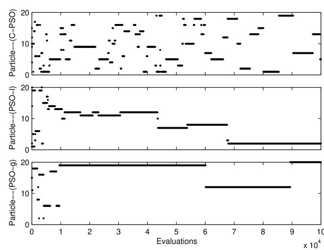
Figure 5.5: Best particle in the swarm of the three PSO algorithms used in parameter identification, C-PSO (top), PSO-l (middle), and PSO-g (bottom)

The alternation of the best particle status as depicted in the C-PSO case shows that most of the particles of the swarm participated effectively in the search process; While some particles are searching for the global optimum in one region, the other particles are searching for that optimum elsewhere, but are guided by the experience of the other particles in the swarm. This effective search mechanism was present but with less efficiency in the case of the PSO-l algorithm, and this efficiency is much more less in the case of the PSO-g as few particles are effectively searching for the global minimum which the others are being dragged by them.

5.5.5 Conclusions

The problem of parameter identification presents quite a challenge for any optimizer due to its multimodality and the availability of constraints. CI techniques are specifically made for such challenging tasks. With their ability to escape local minima and their problem independence they can efficiently exploit the computation power to find the global optimum solution. This superior ability was clear in the presented parameter identification problem as all the CI techniques outperformed the traditional LS techniques used by a big margin.

Among the different CI techniques, two types of algorithms were used. The SI techniques represented by the PSO algorithm and the EA techniques represented by a GA. On average, the PSO variants outperformed the GA regarding final fitness values and convergence speed. One reason for the superiority of the PSO algorithms compared to the GA is its ability to maintain a diverge set of solutions. This was clear when the population of solutions were monitored during the run of the algorithms. The inertia weight used kept the particles reasonable distanced from each other while still being guided by each other. However in the case of the GA optimizer, the most fit individual took-over the population in a relatively small number of generations, and caused most of the population individuals to be almost clones of itself, which badly affected the search process. A possible remedy for this quick take-over effect is increasing the crossover and mutation distribution indexes, however case must be taken because the higher the values of these two parameters the more the algorithm becomes a random search optimizer.

Comparing the different topologies used in the PSO variants, it was found that the C-PSO topology achieved better results regarding all performance metrics used. Further analysis of the obtained results revealed that the dynamic nature of the neighborhood employed in the C-PSO topology resulted in a more efficient search mechanism that employed the efforts of all particles to search different regions of the search space instead of following few particles or even one particle.

Chapter 6 Conclusions

The research presented in this thesis examined the efficiency of CI techniques and some proposed extensions for them. First, it extends the simple GA model and proposes a more biological sound representation which mimics the structure of many living organisms’ chromosomes. This representation which adds more redundant chromosomes to the simple—single-chromosome representation produced marginal benefits regarding diversity of solutions as the number of these redundant chromosomes increased. However the convergence speed deteriorated at the meantime. It was found that the algorithm was effectively optimizing the redundant chromosomes as-well-as the primary ones, and this has caused the slow progress of the optimization process. Although the Polyploid algorithm used outperformed the NSGA-II algorithm, it was clear that the multi-chromosomal representation did not lead to this superior performance because the less the number of redundant chromosomes, the more the algorithm approaches the simple—single-chromosome representation, the more the performance improves.

An extension to the PSO algorithms was presented to address some deficiencies in current models. The proposed dynamic neighborhood structure, in some sense, acts as an intermediate solution to two currently well-known static neighborhood structures. However, the results obtained showed that this proposed dynamic neighborhood offers more than a simple compromise solution between two extremes. The simulations on benchmark problems showed that the proposed C-PSO topology outperforms the other two structures even in the characteristics they excel in. It was found that the dynamic structure used in the C-PSO topology makes better use of the available computation power because almost all the particles took part in the optimization process which was not the case in the other two topologies.

The challenging, highly nonlinear, and multimodal problem of induction motor’s parameter identification exploits the good characteristics of the C-PSO algorithm. When different optimizers were used for this problem, the results obtained sustained previous findings, and offered even more. The C-PSO algorithm outperformed all the other algorithms, including the GA, in all performance measures used by a big margin. Not only did the C-PSO algorithm provide a higher convergence speed, it also provided much lower percentage deviation of the identified parameters from the real ones, and higher reliability as well.

A broad look on the algorithms showed that PSO techniques, in general, provided higher convergence speed, and lower error in the identified parameters, however, the gbest topology presented an exception to this rule. The gbest topology, which is known for its fast convergence speed, was not a good choice for such a highly multimodal problem. This topology leads to premature convergence and causes the algorithm to get trapped very early in the run in a bad local minima, which was not the case with the lbest and C-PSO topologies.

A reason for the relatively inferior performance of the GA was its low take-over time. The algorithm causes the population to lose its diversity and converge rapidly to a single individual although many precautions were taken to alleviate this well-known deficiency of the GA optimizer. On the other hand, the diversity of solutions maintained by the C-PSO and lbest topologies were their winning horse, it allowed them to explore new regions and avoid stagnation even at late stages of the search process.

Artificial intelligence models, and in particular, CI models show promising results in the system identification problem. The results reported in this research answer some questions regarding the suitability of some algorithms to some techniques, however, at the same time they raise many questions to be answered by future research. What could be a possible remedy to the innate deficiency of the GA technique regarding its low take-over time? Should the parents be specifically matched instead of being randomly assigned to each other? Since the dynamic neighborhood structure used in this research for the PSO algorithm resulted in such a significant performance improvement, should other aspects of the algorithm such as inertia weight and learning rates be made dynamic as well? What about dynamic swarm size and multiple swarms? The volume of questions exceeds the limited space of this thesis and spurs more research in the applications and development of the interesting field of AI.

Appendix A Induction Motor Model Derivation

A space phasor x is described as:

$$\underline{x}=x_{d}+jx_{q}$$ (A.1)

Then for a reference frame rotating with speed $\omega_{e}$, the motor stator and rotor voltage equations. are:

$$\underline{v}_{s}^{e} =r_{s}\underline{i}_{s}^{e}+\dot{\underline{\psi}}_{s}^{e}+j\,\omega_{e}\underline{\psi}_{s}^{e}$$ (A.2)

$$\underline{v}_{r}^{e} =0=r_{r}\underline{i}_{r}^{e}+\dot{\underline{\psi}}_{r}^{e}+j\,(\omega_{e}-\omega_{m})\underline{\psi}_{r}^{e}$$

Where $\omega_{m}$ is the electrical rotor speed.

To simplify (A.2), we select a stator reference frame (superscript $s$) which is fixed to the machine stator, i.e. $\omega_{e}=0$, to get:

$$\dot{\psi}_{sd}^{s} =-r_{s}i_{sd}^{s}+v_{sd}^{s}$$ (A.3)

$$\dot{\psi}_{sq}^{s} =-r_{s}i_{sq}^{s}+v_{sq}^{s}$$

$$\dot{\psi}_{rd}^{s} =-r_{r}i_{rd}^{s}-\omega_{m}\psi_{rq}^{s}$$

$$\dot{\psi}_{rq}^{s} =-r_{r}i_{rq}^{s}-\omega_{m}\psi_{rd}^{s}$$

Using

$$\underline{\psi}_{s} =(L_{sl}+L_{m})\underline{i}_{s}+L_{m}\underline{i}_{r}$$ (A.4)

$$\underline{\psi}_{r} =L_{m}\underline{i}_{s}+(L_{rl}+L_{m})\underline{i}_{r}$$

We get

$$\underline{i}_{s} =\frac{L_{rl}+L_{m}}{L_{d}}\underline{\psi_{s}}-\frac{L_{m}}{L_{d}}\underline{\psi}_{r}$$ (A.5)

$$\underline{i}_{r} =-\frac{L_{m}}{L_{d}}\underline{\psi}_{s}+\frac{L_{ls}+L_{m}}{L_{d}}\underline{\psi_{r}}$$

$$L_{d} =L_{sl}L_{rl}+L_{m}(L_{sl}+L_{rl})$$

Using ($d$ - $q$) components of $\underline{\psi}_{s}$, $\underline{\psi}_{r}$ to express ($d$ - $q$) components of $\underline{i}_{s}$, $\underline{i}_{r}$ according to (A.5), then (A.3) becomes:

$$\dot{\psi}_{sd}^{s} =-r_{s}x_{1}\psi_{sd}^{s}+r_{s}\beta\psi_{rd}^{s}+v_{sd}^{s}$$ (A.6)

$$\dot{\psi}_{sq}^{s} =-r_{s}x_{1}\psi_{sq}^{s}+r_{s}\beta\psi_{rq}^{s}+v_{sq}^{s}$$

$$\dot{\psi}_{rd}^{s} =-r_{r}x_{2}\psi_{rd}^{s}+r_{r}\beta\psi_{sd}^{s}+\omega_{m}\psi_{rq}{s}$$

$$\dot{\psi}_{rq}^{s} =-r_{r}x_{2}\psi_{rq}^{s}+r_{r}\beta\psi_{sq}^{s}+\omega_{m}\psi_{rd}{s}$$

$$x_{1} =\frac{L_{rl}+L_{m}}{L_{d}},\quad x_{2}=\frac{L_{ls}+L_{m}}{L_{d}}$$

$$\beta =\frac{L_{m}}{L_{d}}$$

To get d.e. needed to solve for $\omega_{m}$, the generated electromagnetic torque is given by

$$T_{e}=\frac{3P}{2}(i_{sq}\psi_{sd}-i_{sd}\psi_{sq})$$ (A.7)

where

$$i_{sd}=x_{1}\psi_{sd}-\beta\psi_{rd}$$ (A.8)

$$i_{sq}=x_{1}\psi_{sq}-\beta\psi_{rq}$$

$$P=\text{number of pole pairs}$$

and the motor mechanical equation is :

$$J\frac{d\omega^{\prime}_{m}}{dt}=T_{e}-T_{L}-T_{D}$$ (A.9)

where
$\omega^{\prime}_{m}$ : rotor speed in mechanical radian per sec. $T_{L}$ : load torque $T_{D}$ : damping torque

Using $\omega^{\prime}_{m}=\frac{2}{p}\omega_{m}$ and for $T_{L}=T_{D}=0$, we get

$$\frac{d\omega_{m}}{dt}=\frac{3P^{2}}{4J}(i_{sq}\psi_{sd}-i_{sd}\psi_{sq})$$ (A.10)

And the induction motor model is represented by (A.6), (A.8) and (A.10).

To get $v_{sd}^{s}$, $v_{sq}^{s}$ given the line voltages $v_{1}$, $v_{2}$ and $v_{3}$, Park’s transformation is used:

$$\begin{bmatrix}f_{d}\\ f_{q}\\ f_{o}\end{bmatrix}=\frac{2}{3}\begin{bmatrix}\cos(\theta)&\cos(\theta-120)&\cos(\theta+120)\\ -\sin(\theta)&-\sin(\theta-120)&-\sin(\theta+120)\\ \frac{1}{2}&\frac{1}{2}&\frac{1}{2}\end{bmatrix}\begin{bmatrix}f_{a}\\ f_{b}\\ f_{c}\end{bmatrix}$$ (A.11)

Where $f_{o}$ equation is added to yield a unique transformation, and $\theta$ is the electrical angle between the $d$-axis and the stator phase-$a$ axis as shown in Figure A.1:

Figure A.1: Axis transformation

The multiplier $(\frac{2}{3})$ is used to equalize the magnitude of mmf produced in $d$-$q$ frame with that of the 3-phase winding.

For $\theta=0$, then

$$v_{sd}^{s} =\frac{2}{3}(v_{1}+v_{2}\cos(-120)+v_{3}\cos(120))$$ (A.12)

$$=\frac{2}{3}(v_{1}-\frac{1}{2}v_{2}-\frac{1}{2}v_{3})$$

$$=\frac{1}{3}(2v_{1}-v_{2}-v_{3})$$

$$v_{sq}^{s} =\frac{2}{3}(-v_{2}\sin(-120)-v_{3}\sin(120))$$ (A.13)

$$=\frac{2}{3}(\frac{\sqrt{3}}{2}v_{2}-\frac{\sqrt{3}}{2}v_{3})$$

$$=\frac{1}{\sqrt{3}}(v_{2}-v_{3})$$

Also, the inverse transformation

$$\begin{bmatrix}f_{a}\\ f_{b}\\ f_{c}\end{bmatrix}=\begin{bmatrix}\cos(\theta)&-\sin(\theta)&1\\ \cos(\theta-120)&-\sin(\theta-120)&1\\ \cos(\theta+120)&-\sin(\theta+120)&1\end{bmatrix}\begin{bmatrix}f_{d}\\ f_{q}\\ f_{o}\end{bmatrix}$$

is used to get the line currents $i_{1}$, $i_{2}$ and $i_{3}$ given $i_{sd}^{s}$ and $i_{sq}^{s}$ by using $\theta=0$ and $i_{o}=0$,

$$i_{1} =i_{sd}^{s}$$ (A.14)

$$i_{2} =i_{sd}^{s}\cos(-120)-i_{sq}^{s}\sin(-120)$$

$$=-\frac{1}{2}i_{sd}^{s}+\frac{\sqrt{3}}{2}i_{sq}^{s}$$

$$i_{3} =-\frac{1}{2}i_{sd}^{s}-\frac{\sqrt{3}}{2}i_{sq}^{s}$$

and one iteration of the identification algorithm proceeds as follows:

1. Initialize model parameters: $\hat{r}_{s}$, $\hat{r}_{r}$, $\hat{L}_{sl}$, $\hat{L}_{rl}$, $\hat{L}_{m}$ and $\hat{J}$.

2. Get $v_{sd}^{s}$ and $v_{sq}^{s}$ given $v_{1}$, $v_{2}$ and $v_{3}$ using (A.12) and (A.13).

3. Solve (A.6), (A.8), (A.10) for a period of time $T$ .

4. Get $\hat{i}_{sd}^{s}$ and $\hat{i}_{sq}^{s}$ using (A.8).

5. Get $\hat{i}_{1}$, $\hat{i}_{2}$ and $\hat{i}_{3}$ using (A.14).

6. Evaluate the error (fitness function): $f=\int_{0}^{T}(|i_{1}-\hat{i}_{1}|+|i_{2}-\hat{i}_{2}|+|i_{3}-\hat{i}_{3}|)dt$, where $i_{1}$, $i_{2}$ and $i_{3}$ are the true measured line currents over the interval: $t\in[0,T]$.

7. If $f\leq e$ then stop, or else

8. Update the model parameters ($\hat{r}_{s}$, $\hat{r}_{r}$, $\hat{L}_{sl}$, $\hat{L}_{rl}$, $\hat{L}_{m}$ and $\hat{J}$) using one of the optimizers mentioned in Chapter 5, then go to step 3.

An alternative model is used to represent the induction motor dynamics, especially for indirect field-oriented control applications as well as on-line identification of the rotor resistance [145], is given as follows:

$$\dot{x} =Ax+Bu$$ (A.15)

$$x =[i_{sd}~{}i_{sq}~{}\lambda_{rd}~{}\lambda_{rq}]^{T}$$

$$u =[v_{sd}~{}v_{sq}~{}0~{}0]^{T}$$

$$A =\begin{bmatrix}-\gamma&0&\mu\>\eta&\mu\>\omega_{m}\\ 0&\gamma&-\mu\>\omega_{m}&\mu\>\eta\\ \eta L_{m}&0&-\eta&-\omega_{m}\\ 0&\eta L_{m}&\omega_{m}&-\eta\end{bmatrix}$$

$$B =\begin{bmatrix}\frac{1}{\sigma L_{s}}\\ \frac{1}{\sigma L_{s}}\\ 0\\ 0\end{bmatrix}$$

where

$$\eta =\frac{r_{r}}{L_{r}}$$ (A.16)

$$\sigma =\frac{L_{s}L_{r}-L_{m}^{2}}{L_{s}L_{r}}=\text{the total leakage factor}$$

$$\gamma =\frac{1}{L_{r}(L_{s}L_{r}-L_{m}^{2})}(r_{s}L_{r}^{2}+r_{r}L_{m}^{2})$$

$$\mu =\frac{L_{m}}{L_{s}L_{r}-L_{m}^{2}}$$

$$L_{s} =L_{sl}+L_{m}$$

$$L_{r} =L_{rl}+L_{m}$$

To show how to derive this model from the previous one we start by:

$$v_{sd} =r_{s}i_{sd}+\dot{\psi}_{sd}$$ (A.17)

$$v_{sq} =r_{s}i_{sq}+\dot{\psi}_{sq}$$

$$0 =r_{r}i_{rd}+\dot{\psi}_{rd}+\omega_{m}\psi_{rq}$$

$$0 =r_{r}i_{rq}+\dot{\psi}_{rq}-\omega_{m}\psi_{rd}$$

$$\underline{\psi}_{s} =L_{s}\underline{i}_{s}+L_{m}\underline{i}_{r}$$ (A.18)

$$\underline{\psi}_{r} =L_{m}\underline{i}_{s}+L_{r}\underline{i}_{r}$$

$$L_{s} =L_{sl}+L_{m}$$

$$L_{r} =L_{rl}+L_{m}$$

Starting by:

$$\dot{\psi}_{rd}=-r_{r}i_{rd}-\omega_{m}\psi_{rq}$$

using

$$\psi_{rd} =L_{m}i_{sd}+L_{r}i_{rd}$$

$$\therefore i_{rd} =\frac{1}{L_{r}}\psi_{rd}-\frac{L_{m}}{L_{r}}i_{sd}$$

$$\therefore\dot{\psi}_{rd} =\frac{r_{r}L_{m}}{L_{r}}i_{sd}-\frac{r_{r}}{L_{r}}\psi_{rd}-\omega_{m}\psi_{rq}$$

and the same steps are followed to get the $\dot{\psi}_{rq}$ equation.

Now considering:

$$\dot{\psi}_{sd}=-r_{s}i_{sd}+v_{sd}$$

using (A.18), we get:

$$\begin{bmatrix}i_{sd}\\ i_{rd}\end{bmatrix}=\frac{1}{L_{s}L_{r}-L_{m}^{2}}\begin{bmatrix}L_{r}&-L_{m}\\ -L_{m}&L_{s}\end{bmatrix}\begin{bmatrix}\psi_{sd}\\ \psi_{rd}\end{bmatrix}$$

and

$$i_{sd} =\frac{L_{r}}{L_{s}L_{r}-L_{m}^{2}}\psi_{sd}-\frac{L_{m}}{L_{s}L_{r}-L_{m}^{2}}\psi_{rd}$$

$$=\frac{1}{\sigma L_{s}}\psi_{sd}-\mu\>\psi_{rd}$$

differentiating, we get:

$$\dot{i}_{sd} =\frac{1}{\sigma L_{s}}\dot{\psi}_{sd}-\mu\>\dot{\psi}_{rd}$$

$$=\frac{1}{\sigma L_{s}}(-r_{s}i_{sd}+v_{sd})-\mu(-r_{r}i_{rd}-\omega_{m}\psi_{rq})$$

using

$$i_{rd}=\frac{1}{L_{r}}\psi_{rd}-\frac{L_{m}}{L_{r}}i_{sd}$$

then

$$\dot{i}_{sd}=-\frac{r_{s}}{\sigma L_{s}}i_{sd}+\mu\>r_{r}(\frac{1}{L_{r}}\psi_{rd}-\frac{L_{m}}{L_{r}}i_{sd})+\mu\>\omega_{m}\psi_{rq}+\frac{1}{\sigma L_{s}}v_{sd}$$ (A.19)

i.e.

$$\dot{i}_{sd}=-(\frac{r_{s}}{\sigma L_{s}}+\frac{\mu\>r_{r}L_{m}}{L_{r}})i_{sd}+\frac{\mu\>r_{r}}{L_{r}}\psi_{rd}+\mu\>\omega_{m}\psi_{rq}+\frac{1}{\sigma L_{s}}v_{sd}$$ (A.20)

where

$$\frac{r_{s}}{\sigma L_{s}}+\frac{\mu\>r_{r}L)m}{L_{r}} =\frac{r_{s}L_{s}L_{r}}{(L_{s}L_{r}-L_{m}^{2})L_{s}}+\frac{L_{m}^{2}r_{r}}{(L_{s}L_{r}-L_{m}^{2})L_{r}}$$ (A.21)

$$=\frac{1}{L_{s}L_{r}-L_{m}^{2}}(r_{s}L_{r}+\frac{L_{m}^{2}r_{r}}{L_{r}})$$

$$=\gamma$$

i.e.

$$\dot{i}_{sd}=-\gamma\>i_{sd}+\mu\>\eta\psi_{rd}+\mu\>\omega_{m}\psi_{rq}+\frac{1}{\sigma L_{s}}v_{sd}$$ (A.22)

and following the same steps, we get the equation for $\dot{i}_{sq}$

Now for the torque equation, using

$$v_{sd}=\sigma L_{s}\dot{i}_{sd}+\gamma\>i_{sd}-\mu\>\eta\sigma L_{s}\psi_{rd}-\sigma L_{s}\omega_{m}\mu\>\psi_{rq}$$

$$v^{\prime}_{sd} =-\sigma L_{s}\omega_{m}\eta\>\psi_{rq}$$ (A.23)

$$=-\frac{L_{m}}{L_{r}}\omega_{m}\psi_{rq}$$

where $v^{\prime}_{sd}$ is the component of $v_{sd}$ contributing to the output mechanical power.

Also,

$$v^{\prime}_{sq}=\frac{L_{m}}{L_{r}}\omega_{m}\psi_{rd}$$ (A.24)

using

$$P_{m}=T\frac{\omega_{m}}{P} =\frac{3}{2}(v^{\prime}_{sd}i_{sd}+v^{\prime}_{sq}i_{sq})$$ (A.25)

$$=\frac{3}{2}\omega_{m}\frac{L_{m}}{L_{r}}(\psi_{rd}i_{sq}-\psi_{rq}i_{sd})$$

i.e.

$$T =\frac{3P}{2}\cdot\frac{L_{m}}{L_{r}}(\psi_{rd}i_{sq}-\psi_{rq}i_{sd})$$

$$=\frac{J}{P}\dot{\omega}_{m}+\frac{\beta}{P}\omega_{m}+T_{L}$$

i.e.

$$\dot{\omega}_{m}=\frac{3P^{2}}{2J}\cdot\frac{L_{m}}{L_{r}}(\psi_{rd}i_{sq}-\psi_{rq}i_{sd})-\frac{\beta}{J}\omega_{m}-\frac{P}{J}T_{L}$$ (A.26)

where

$P$ :	no. of pole-pairs
$\omega_{m}$ :	rotor speed in electrical rad./s
$J$ :	rotor moment of inertia
$\beta$ :	viscous damping coefficient
$T_{L}$ :	load torque
$P_{m}$ :	gross generated mechanical power

References

- [1] P. J. Fleming and R. C. Purshouse, “Genetic algorithms in control systems engineering,” Department of Automatic Control and Systems Engineering, University of Sheffield, Sheffield, UK, Tech. Rep. 789, May 2001, http://citeseer.ist.psu.edu/fleming01genetic.html.
- [2] N. Bohr, “On the constitution of atoms and molecules,” Philosophical Magazine, vol. 26, no. 151, pp. 1–25, 1913.
- [3] G. P. Liu, J. B. Yang, and J. F. Whidborne, Multiobjective Optimisation and Control. Baldock, England: Research Studies Press Ltd., 2003.
- [4] E. Zitzler, “Evolutionary Algorithms for Multiobjective Optimization: Methods and Applications,” Ph.D. dissertation, Swiss Federal Institute of Technology (ETH), Zurich, Switzerland, Nov. 1999.
- [5] A. Törn and A. Zilinskas, Global Optimization. Berlin: Springer, 1989.
- [6] H. Muhlenbein, M. Schomisch, and J. Born, “The parallel genetic algorithm as function optimizer,” Parallel Computing, vol. 17, pp. 619–632, 1991.
- [7] J. D. Schaffer, “Multiple objective optimization with vector evaluated genetic algorithms,” in Proceedings of the 1st International Conference on Genetic Algorithms (ICGA), J. J. Grefenstette, Ed. PA, USA: Lawrence Erlbaum Associates, Jul. 1985, pp. 93–100.
- [8] D. A. van Veldhuizen and G. B. Lamont, “Multiobjective evolutionary algorithm test suites,” in Symposium on Applied Computing, 1999, pp. 351–357, http://citeseer.ist.psu.edu/289907.html.
- [9] R. C. Purshouse and P. J. Fleming, “conflict, harmony, and independence: Relationships in evolutionary multi-criterion optimisation,” in Proceedings of Evolutionary Multi-Criterion Optimization. Second International Conference, EMO 2003, C. M. Fonseca, P. J. Fleming, E. Zitzler, K. Deb, and L. Thiele, Eds., vol. 2632. Faro, Portugal: Springer. Lecture Notes in Computer Science, Apr. 2003, pp. 16–30, http://www.lania.mx/~ccoello/EMOO/purshouse03.pdf.gz.
- [10] C. L. Hwang and A. S. M. Masud, Multiple Objective Decision Making - Methods and Applications, ser. Lecture Notes in Economics and Mathematical Systems. Springer-Verlag, 1979, vol. 164.
- [11] R. E. Steuer, Multiple Criteria Optimization : Theory, Computation, and Application. New York, Toronto: Wiley, 1986.
- [12] V. Pareto, Cours D’Economie Politique. Lausanne: F. Rouge, 1896.
- [13] Wikipedia, “Timeline of algorithms,” 2007, http://en.wikipedia.org/w/index.php?title=Timeline_of_algorithms&oldid=%99249593.
- [14] D. H. Wolpert and W. G. Macready, “No free lunch theorems for search,” Santa Fe Institute, Santa Fe, NM, Tech. Rep. SFI-TR-95-02-010, 1995, http://citeseer.ist.psu.edu/wolpert95no.html.
- [15] Z. Michalewicz and D. B. Fogel, How to Solve It: Modern Heuristics. Berlin: Springer, 2000.
- [16] W. G. Macready and D. H. Wolpert, “What makes an optimization problem hard?” Santa Fe Institute, Santa Fe, NM, Tech. Rep. SFI-TR-95-05-046, 1995, http://citeseer.ist.psu.edu/macready96what.html.
- [17] T. Jones and S. Forrest, “Fitness distance correlation as a measure of problem difficulty for genetic algorithms,” in Proceedings of the Sixth International Conference on Genetic Algorithms, L. Eshelman, Ed. San Francisco, CA: Morgan Kaufmann, 1995, pp. 184–192, http://citeseer.ist.psu.edu/jones95fitness.html.
- [18] P. F. Stadler, “Towards a theory of landscapes,” in Complex Systems and Binary Networks, R. Lopéz-Peña, R. Capovilla, R. García-Pelayo, H. Waelbroeck, and F. Zertuche, Eds., vol. 461. Berlin, New York: Springer Verlag, 1995, pp. 77–163, http://citeseer.ist.psu.edu/stadler95towards.html.
- [19] B. Naudts and L. Kallel, “A comparison of predictive measures of problem difficulty in evolutionary algorithms,” IEEE Trans. on Evolutionary Computation, vol. 4, no. 1, p. 1, Apr. 2000, http://citeseer.ist.psu.edu/naudts00comparison.html.
- [20] M. Jelasity, B. Tóth, and T. Vinkó, “Characterizations of trajectory structure of fitness landscapes based on pairwise transition probabilities of solutions,” in Proceedings of the 1999 Congress on Evolutionary Computation (CEC 99), IEEE. Piscataway, NJ: IEEE Press, 1999, pp. 623–630, http://citeseer.ist.psu.edu/jelasity99characterizations.html.
- [21] M. Mitchell, S. Forrest, and J. H. Holland, “The royal road for genetic algorithms: Fitness landscapes and GA performance,” in Towards a Practice of Autonomous Systems: Proceedings of the First European Conference on Artificial Life, 1991, F. J. Varela and P. Bourgine, Eds. Paris: A Bradford book, The MIT Press, 1992, pp. 245–254, http://citeseer.ist.psu.edu/mitchell91royal.html.
- [22] S. Forrest and M. Mitchell, “What makes a problem hard for a genetic algorithm? some anomalous results and their explanation,” Machine Learning, vol. 13, pp. 285–319, 1993, http://citeseer.ist.psu.edu/forrest93what.html.
- [23] A. H. Wright, R. K. Thompson, and J. Zhang, “The computational complexity of n-k fitness functions,” IEEE Trans. on Evolutionary Computation, vol. 4, no. 4, p. 373, Nov. 2000, http://citeseer.ist.psu.edu/wright99computational.html.
- [24] J. He, X. Yao, and Q. Zhang, “To understand one-dimensional continuous fitness landscapes by drift analysis,” in Proceedings of the 2004 IEEE Congress on Evolutionary Computation (CEC 04). Portland, Oregon: IEEE Press, Jun. 2004, pp. 1248–1253, http://www.cs.bham.ac.uk/~jxh/2004cec.pdf.
- [25] H. Guo and W. H. Hsu, “Ga-hardness revisited,” in GECCO, ser. Lecture Notes in Computer Science, E. Cantú-Paz, J. A. Foster, K. Deb, L. Davis, R. Roy, U.-M. O’Reilly, H.-G. Beyer, R. K. Standish, G. Kendall, S. W. Wilson, M. Harman, J. Wegener, D. Dasgupta, M. A. Potter, A. C. Schultz, K. A. Dowsland, N. Jonoska, and J. F. Miller, Eds., vol. 2724. Springer, 2003, pp. 1584–1585, http://citeseer.ist.psu.edu/guo03gahardness.html.
- [26] M. Davis and H. Putnam, “A computing procedure for quantification theory,” J. ACM, vol. 7, no. 3, pp. 201–215, 1960.
- [27] D. E. Goldberg, “Simple genetic algorithms and the minimal, deceptive problem,” in Genetic Algorithms and Simulated Annealing. Morgan Kaufmann, 1987, pp. 74–88.
- [28] L. D. Whitley, “Fundamental principles of deception in genetic search,” in Foundations of genetic algorithms, G. J. Rawlins, Ed. San Mateo, CA: Morgan Kaufmann, 1991, pp. 221–241, http://citeseer.ist.psu.edu/whitley91fundamental.html.
- [29] D. E. Goldberg, K. Deb, and J. Horn, “Massive multimodality, deception, and genetic algorithms,” University of Illinois, Urbana, Tech. Rep. IlliGAL Report No 92005, 1992, ftp://gal2.ge.uiuc.edu/pub/papers/IlliGALs/92005.ps.z.
- [30] J. J. Grefenstette, “Deception considered harmful,” in Foundations of Genetic Algorithms 2, L. D. Whitley, Ed. San Mateo, CA: Morgan Kaufmann, 1993, pp. 75–91, http://citeseer.ist.psu.edu/grefenstette92deception.html.
- [31] J. Horn and D. E. Goldberg, “Genetic algorithm difficulty and the modality of fitness landscapes,” in Foundations of Genetic Algorithms 3, L. D. Whitley and M. D. Vose, Eds. San Francisco, CA: Morgan Kaufmann, 1995, pp. 243–269, http://citeseer.ist.psu.edu/horn94genetic.html.
- [32] G. Singh and K. Deb, “Comparison of multi-modal optimization algorithms based on evolutionary algorithms,” in GECCO, M. Cattolico, Ed. ACM, 2006, pp. 1305–1312, http://www.cs.bham.ac.uk/~wbl/biblio/gecco2006/docs/p1305.pdf.
- [33] K. Kolarov, “Landscape ruggedness in evolutionary algorithms,” in IEEECEP: Proceedings of The IEEE Conference on Evolutionary Computation, IEEE World Congress on Computational Intelligence, 1997, http://citeseer.ist.psu.edu/kolarov97landscape.html.
- [34] L. Kallel, B. Naudts, and C. R. Reeves, “Properties of fitness functions and search landscapes,” in Theoretical Aspects of Evolutionary Computing, L. Kallel, B. Naudts, and A. Rogers, Eds. Berlin: Springer, 2001, pp. 175–206, http://citeseer.ist.psu.edu/kallel01properties.html.
- [35] C. Darwin, On the Origin of Species. London: John Murray, 1859, http://embryology.med.unsw.edu.au/pdf/Origin_of_Species.pdf.
- [36] G. E. P. Box, “Evolutionary operation: A method for increasing industrial productivity,” Applied Statistics, vol. 6, no. 2, pp. 81–101, 1957.
- [37] I. Rechenberg, “Cybernetic solution path of an experimental problem,” Royal Air Force Establishment, Tech. Rep., 1965.
- [38] J. D. Bagley, “The behavior of adaptive systems which employ genetic and correlation algorithms,” Ph.D. dissertation, University of Michigan, 1967.
- [39] J. H. Holland, Adaptation in Natural and Artificial Systems: An Introductory Analysis with Applications to Biology, Control, and Artificial Intelligence. University of Michigan, 1975.
- [40] K. A. De Jong, “An analysis of the behavior of a class of genetic adaptive systems,” Ph.D. dissertation, University of Michigan, Ann Arbor, 1975, http://cs.gmu.edu/~eclab/kdj_thesis.html.
- [41] G. Levitin, Ed., Computational Intelligence in Reliability Engineering, ser. Studies in Computational Intelligence. Berlin: Springer, Jan. 2007, vol. 39.
- [42] J. Wang and A. Kusiak, Eds., Computational Intelligence in Manufacturing Handbook, ser. Handbook Series for Mechanical Engineering. FL, USA: CRC Press LLC, Dec. 2000, vol. 5.
- [43] T. Bäck, F. Hoffmeister, and H.-P. Schwefel, “Applications of evolutionary algorithms,” Systems Analysis Research Group, University of Dortmund, Dortmund, Germany, Tech. Rep. SYS-2/92, 1992, http://citeseer.ist.psu.edu/back93applications.html.
- [44] C. L. Karr and L. M. Freeman, Eds., Industrial Applications of Genetic Algorithms. Boca Raton, FL: CRC Press, 1999.
- [45] P. A. N. Bosman and T. Alderliesten, “Evolutionary algorithms for medical simulations: a case study in minimally-invasive vascular interventions,” in GECCO Workshops, F. Rothlauf, Ed. ACM, 2005, pp. 125–132.
- [46] L. D. Chambers, Practical Handbook of Genetic Algorithms. Boca Raton, FL, USA: CRC Press, Inc., 1995.
- [47] S. Geisendorf, “Genetic algorithms in resource economic models,” Santa Fe Institute, NM, USA, Working Papers 99-08-058, Aug. 1999, http://www.santafe.edu/research/publications/workingpapers/99-08-058.ps%.
- [48] T. Bäck, U. Hammel, and H.-P. Schwefel, “Evolutionary computation: Comments on the history and current state,” IEEE Trans. on Evolutionary Computation, vol. 1, no. 1, pp. 3–17, 1997, http://citeseer.ist.psu.edu/601414.html.
- [49] D. Fogel, Ed., Evolutionary Computation: The Fossil Record. NY: IEEE Press, 1998.
- [50] K. De Jong, D. B. Fogel, and H.-P. Schwefel, “A history of evolutionary computation,” in Evolutionary Computation 1: Basic Algorithms and Operators, T. Bäck, D. B. Fogel, and Z. Michalewicz, Eds. Bristol: Institute of Physics Publishing, 2000, pp. 40–58.
- [51] L. J. Fogel, A. J. Owens, and M. J. Walsh, Artificial Intelligence Through Simulated Evolution. New York: John Wiley & Sons, 1966.
- [52] J. R. Koza, “Hierarchical genetic algorithms operating on populations of computer programs,” in Proceedings of the 11th International Joint Conference on Artificial Intelligence. Morgan Kaufmann Publishers, Inc., 1989, pp. 768–774, http://www.genetic-programming.com/jkpdf/ijcai1989.pdf.
- [53] ——, Genetic Programming: On the Programming of Computers by Means of Natural Selection. Cambridge, MA, USA: MIT Press, 1992.
- [54] D. E. Goldberg, Genetic Algorithms in Search, Optimization and Machine Learning. Addison Wesley, 1989.
- [55] J. H. Holland, K. J. Holyoak, R. E. Nisbett, and P. R. Thagard, Induction: Process of Inference, Learning and Discovery. MIT Press, 1986.
- [56] T. Bäck, “Introduction to evolutionary algorithms,” in Evolutionary Computation 1: Basic Algorithms and Operators, T. Bäck, D. B. Fogel, and Z. Michalewicz, Eds. Bristol: Institute of Physics Publishing, 2000, pp. 59–63.
- [57] J. H. Holland, “Outline for a logical theory of adaptive systems,” J. ACM, vol. 9, no. 3, pp. 297–314, 1962.
- [58] H. A. Simon and A. Newell, “Heuristic problem solving: The next advance in operations research,” Operations Research, vol. 6, pp. 1–10, 1958.
- [59] A. Newell, J. C. Shaw, and H. A. Simon, “Report on a general problem-solving program for a computer,” in Information processing: proc. intl. conf. on information processing (IFIP 60). Paris: UNESCO, 1959, pp. 256–264.
- [60] C. C. Gotlieb, “General-purpose programming for business applications,” Advances in Computers, vol. 1, pp. 1–42, 1960.
- [61] W. M. Spears, Evolutionary Algorithms: The Role of Mutation and Recombination. Berlin: Springer, 2000.
- [62] A. Schrijver, “On the history of combinatorial optimization (till 1960),” in Handbook of Discrete Optimization, K. Aardal, G. Nemhauser, and R. Weismantel, Eds. Amsterdam: Elsevier, Jul. 2005, pp. 1–68, http://citeseer.ist.psu.edu/466877.html.
- [63] M. Mitchell, An Introduction to Genetic Algorithms. Cambridge, MA: MIT Press, 1996.
- [64] C. W. Ahn, Advances in Evolutionary Algorithms: Theory, Design and Practice, ser. Studies in Computational Intelligence. Berlin: Springer, 2006, vol. 18.
- [65] A. E. Eiben and J. E. Smith, Introduction to Evolutionary Computing, ser. Natural Computing. Berlin: Springer-Verlag, 2003.
- [66] P. J. Hancock, “Selection methods for evolutionary algorithms,” in Practical Handbook of Genetic Algorithms: New Frontiers, L. Chambers, Ed. FL, USA: CRC Press, 1995, vol. 2, ch. 3, pp. 67–92.
- [67] T. Bäck, Evolutionary Algorithms in Theory and Practice. New York: Oxford University Press, 1996.
- [68] T. Bäck, D. B. Fogel, and Z. Michalewicz, Eds., Evolutionary Computation 1: Basic Algorithms and Operators. Bristol: Institute of Physics Publishing, 2000.
- [69] K. Deb and R. B. Agrawal, “Simulated binary crossover for continuous search space,” Complex Systems, vol. 9, pp. 115–148, 1995, http://citeseer.ist.psu.edu/deb95simulated.html.
- [70] L. B. Booker, D. B. Fogel, D. Whitley, P. J. Angeline, and A. E. Eiben, “Recombination,” in Evolutionary Computation 1: Basic Algorithms and Operators, T. Bäck, D. B. Fogel, and Z. Michalewicz, Eds. Bristol: Institute of Physics Publishing, 2000, ch. 33, pp. 256–307.
- [71] G. Mendel, “Experiments in plant hybridization.” Bohemia: Brünn Natural History Society, Feb. 1865, http://www.esp.org/foundations/genetics/classical/gm-65.pdf.
- [72] A. E. Eiben and C. A. Schippers, “On evolutionary exploration and exploitation,” Fundamenta Informaticae, vol. 35, no. 1-4, pp. 35–50, 1998, http://citeseer.ist.psu.edu/eiben98evolutionary.html.
- [73] B. Naudts and A. Schippers, “A motivated definition of exploitation and exploration,” in Proceedings of the Genetic and Evolutionary Computation Conference (GECCO99), W. Banzhaf, J. Daida, A. E. Eiben, M. H. Garzon, V. Honavar, M. Jakiela, and R. E. Smith, Eds., vol. 1. Orlando, Florida, USA: Morgan Kaufmann, 1999, pp. 800–801, http://citeseer.ist.psu.edu/113441.html.
- [74] K. Deb and H.-G. Beyer, “Self-adaptive genetic algorithms with simulated binary crossover,” University of Dortmund, Dortmund, Germany, Tech. Rep. CI-61/99, Mar. 1999, http://citeseer.ist.psu.edu/deb99selfadaptive.html.
- [75] D. J. Montana and L. Davis, “Training feedforward neural networks using genetic algorithms,” in IJCAI, 1989, pp. 762–767, http://vishnu.bbn.com/papers/ijcai89.pdf.
- [76] T. Back, D. B. Fogel, D. Whitley, and P. J. Angeline, “Mutation operators,” in Evolutionary Computation 1: Basic Algorithms and Operators, T. Bäck, D. B. Fogel, and Z. Michalewicz, Eds. Bristol: Institute of Physics Publishing, 2000, ch. 32, pp. 237–255.
- [77] M. M. Raghuwanshi and O. G. Kakde, “Survey on multiobjective evolutionary and real coded genetic algorithms.” Cairns, Australia: Monash University, Dec. 2004, pp. 150–161, http://www.complexity.org.au/conference/upload/raghuw01/raghuw01.pdf.
- [78] Z. Michalewicz, Genetic Algorithms + Data Structures = Evolution Programs, 3rd ed. Berlin: Springer-Verlag, 1996.
- [79] D. E. Goldberg and R. E. Smith, “Nonstationary function optimization using genetic algorithms with dominance and diploidy,” in Genetic Algorithms and their Applications: Proceedings of the Second International Conference on Genetic Algorithms. Lawrence Erlbaum, 1987, pp. 59–68, ftp://ftp-illigal.ge.uiuc.edu/pub/papers/Publications/1987/nonstationar%y_function_opt-ICGA_1987.pdf.
- [80] R. B. Hollstien, “Artificial genetic adaptation in computer control systems,” Ph.D. dissertation, The University of Michigan, 1971.
- [81] K. P. Ng and K. C. Wong, “A new diploid scheme and dominance change mechanism for non-stationary function optimization,” in Proceedings of the Sixth International Conference on Genetic Algorithms, L. Eshelman, Ed. San Francisco, CA: Morgan Kaufmann, 1995, pp. 159–166.
- [82] R. Cavill, S. L. Smith, and A. M. Tyrrell, “Multi-chromosomal genetic programming,” in GECCO, H.-G. Beyer and U.-M. O’Reilly, Eds. ACM, 2005, pp. 1753–1759, http://www.cs.bham.ac.uk/~wbl/biblio/gecco2005/docs/p1753.pdf.
- [83] S. Massebeuf, C. Fonteix, L. N. Kiss, I. Marc, F. Pla, and K. Zaras, “Multicriteria optimization and decision engineering of an extrusion process aided by a diploid genetic algorithm,” in Proceedings of the Congress on Evolutionary Computation, P. J. Angeline, Z. Michalewicz, M. Schoenauer, X. Yao, and A. Zalzala, Eds., vol. 1. Washington D.C., USA: IEEE Press, 1999, pp. 14–21, http://citeseer.ist.psu.edu/massebeuf99multicriteria.html.
- [84] V. Khare, X. Yao, and K. Deb, “Performance scaling of multi-objective evolutionary algorithms,” in Evolutionary Multi-Criterion Optimization. Second International Conference, EMO 2003, ser. LNCS, C. M. Fonseca, P. J. Fleming, E. Zitzler, K. Deb, and L. Thiele, Eds.
- [85] K. Deb, L. Thiele, M. Laumanns, and E. Zitzler, “Scalable multi-objective optimization test problems,” in Congress on Evolutionary Computation (CEC’2002), vol. 1. Piscataway, New Jersey: IEEE Service Center, May 2002, pp. 825–830, http://citeseer.ist.psu.edu/deb02scalable.html.
- [86] A. M. Turing, “Computing machinery and intelligence,” Mind, vol. 59, no. 236, pp. 433–60, Oct. 1950, http://www.cs.umbc.edu/471/papers/turing.pdf.
- [87] A. Colorni, M. Dorigo, and V. Maniezzo, “Distributed optimization by ant colonies,” in Proceedings of the First European Conference on Artificial Life (ECAL), F. Varela and P. Bourgine, Eds. MIT Press, Cambridge, Massachusetts, 1991, pp. 134–142, http://www.cs.ualberta.ca/~bulitko/F02/papers/IC.06-ECAL92.pdf.
- [88] J. Kennedy and R. C. Eberhart, “Particle swarm optimization,” in Proceedings of the 1995 IEEE International Conference on Neural Networks, vol. 4, Perth, Australia, IEEE Service Center, Piscataway, NJ, 1995, pp. 1942–1948, http://www-sigproc.eng.cam.ac.uk/research/reading%20group/material/The%%20Kalman%20Swarm.pdf.
- [89] A. Abraham, H. Guo, and H. Liu, “Swarm intelligence: Foundations, perspectives and applications,” in Swarm Intelligent Systems, ser. Studies in Computational Intelligence, N. Nedjah and L. de Macedo Mourelle, Eds. Berlin: Springer, Aug. 2006, vol. 26, http://citeseer.ist.psu.edu/737637.html.
- [90] Y. Altshuler, V. Yanovsky, I. Wagner, and A. Bruckstein, “Swarm intelligence—searchers, cleaners and hunters,” in Swarm Intelligent Systems, ser. Studies in Computational Intelligence, N. Nedjah and L. de Macedo Mourelle, Eds. Berlin: Springer, Aug. 2006, vol. 26, http://www.cs.technion.ac.il/people/yanival/online-publications/SI-Book%2006.pdf.
- [91] M. Fleischer, “Foundations of swarm intelligence: From principles to practice,” in Proceddings of Swarming: Network Enabled C4ISR, McLean, VA, Jan. 2005, http://arxiv.org/abs/nlin/0502003.
- [92] J. Kennedy, R. C. Eberhart, and Y. Shi, Swarm Intelligence, ser. Evolutionary Computation Series. San Francisco: Morgan Kaufman, 2001.
- [93] J. M. Bishop, “Stochastic searching networks,” in Proc. 1st IEE Conf. Artificial Neural Networks, London, 1989, pp. 329–331, http://www.cs-cyb-ee.rdg.ac.uk/common/publications/00524.pdf.
- [94] M. Dorigo and L. M. Gambardella, “Ant colony system: A cooperative learning approach to the traveling salesman problem,” IEEE Trans. on Evolutionary Computation, vol. 1, no. 1, pp. 53–66, Apr. 1997, http://citeseer.ist.psu.edu/article/dorigo96ant.html.
- [95] V. Maniezzo and A. Colorni, “The ant system applied to the quadratic assignment problem,” Knowledge and Data Engineering, vol. 11, no. 5, pp. 769–778, 1999, http://citeseer.ist.psu.edu/maniezzo94ant.html.
- [96] R. Schoonderwoerd, O. E. Holland, J. L. Bruten, and L. J. M. Rothkrantz, “Ant-based load balancing in telecommunications networks,” Adaptive Behavior, no. 2, pp. 169–207, 1996, http://citeseer.ist.psu.edu/schoonderwoerd96antbased.html.
- [97] J. Toner and Y. Tu, “Flocks, herds, and schools: A quantitative theory of flocking,” Phys. Rev. E, vol. 58, no. 4, pp. 4828–4858, Oct. 1998, http://arxiv.org/abs/cond-mat/9804180.
- [98] H. Tanner, A. Jadbabaie, and G. J. Pappas, “Stable flocking of mobile agents, part I: Fixed topology,” in Proceedings of the 42nd IEEE Conference on Decision and Control. Maui, HI: IEEE, Dec. 2003, http://citeseer.ist.psu.edu/561802.html.
- [99] ——, “Stable flocking of mobile agents, part II: Dynamic topology,” in Proceedings of the 42nd IEEE Conference on Decision and Control. Maui, HI: IEEE, Dec. 2003, http://citeseer.ist.psu.edu/563430.html.
- [100] J. Kennedy, “Particle swarms: Optimization based on sociocognition,” in Recent Developments in Biologically Inspired Computing, L. N. de Castro and F. J. V. Zuben, Eds. Hershey, PA: Idea Group, 2005, ch. 10.
- [101] A. M. Sutton, D. Whitley, M. Lunacek, and A. Howe, “PSO and multi-funnel landscapes: how cooperation might limit exploration,” in GECCO, M. Cattolico, Ed. ACM, 2006, pp. 75–82, http://www.cs.bham.ac.uk/~wbl/biblio/gecco2006/docs/p75.pdf.
- [102] C. W. Reynolds, “Flocks, herds, and schools: A distributed behavioral model,” Computer Graphics, vol. 21, no. 4, pp. 25–34, 1987, http://www.cs.umu.se/kurser/TDBD12/HT02/papers/ReynoldsBoids1987.pdf.
- [103] A. Ratnaweera, S. K. Halgamuge, and H. C. Watson, “Self-organizing hierarchical particle swarm optimizer with time-varying acceleration coefficients,” IEEE Trans. on Evolutionary Computation, vol. 8, no. 3, pp. 240–255, Jun. 2004.
- [104] Y. Shi and R. C. Eberhart, “Parameter selection in particle swarm optimization,” in Proceedings of the 7th International Conference on Evolutionary Programming VII. London, UK: Springer-Verlag, 1998, pp. 591–600, http://www.engr.iupui.edu/~shi/PSO/Paper/EP98/psof6/ep98_pso.html.
- [105] A. S. Mohais, R. Mendes, C. Ward, and C. Posthoff, “Neighborhood re-structuring in particle swarm optimization,” in Australian Conference on Artificial Intelligence, ser. Lecture Notes in Computer Science, S. Zhang and R. Jarvis, Eds., vol. 3809. Sydney, Australia: Springer, Dec. 2005, pp. 776–785, http://www.di.uminho.pt/~rcm/publications/AI-544.pdf.
- [106] S. Pasupuleti and R. Battiti, “The gregarious particle swarm optimizer (G-PSO),” in GECCO, M. Cattolico, Ed. ACM, 2006, pp. 67–74, http://www.cs.bham.ac.uk/~wbl/biblio/gecco2006/docs/p67.pdf.
- [107] S. Janson and M. Middendorf, “A hierarchical particle swarm optimizer and its adaptive variant,” IEEE Transactions on Systems, Man, and Cybernetics, Part B, vol. 35, no. 6, pp. 1272–1282, 2005, http://pacosy.informatik.uni-leipzig.de/pv/Forschung/Papers/ieee-hierac%hicalPSO.pdf.
- [108] J. Kennedy, “Small worlds and mega-minds: effects of neighborhood topology,” in Proceedings of the 1999 Congress on Evolutionary Computation (CEC 99). Piscataway, NJ: IEEE Press, 1999, pp. 1931–1938.
- [109] E. S. Correa, A. A. Freitas, and C. G. Johnson, “A new discrete particle swarm algorithm applied to attribute selection in a bioinformatics data set,” in GECCO, M. Cattolico, Ed. ACM, 2006, pp. 35–42, http://www.cs.bham.ac.uk/~wbl/biblio/gecco2006/docs/p35.pdf.
- [110] M. Clerc and J. Kennedy, “The particle swarm - explosion, stability, and convergence in a multidimensional complex space,” IEEE Trans. on Evolutionary Computation, vol. 6, pp. 58–73, Feb. 2002, http://clerc.maurice.free.fr/pso/TEC.zip.
- [111] W. Elshamy, H. Emara, and A. Bahgat, “Clubs-based particle swarm optimization,” in Proceedings of the IEEE Swarm Intelligence Symposium 2007 (SIS07), IEEE. Honolulu, HI: IEEE Press, Apr. 2007, http://wesamelshamy.googlepages.com/C_PSO_sis2007.pdf.
- [112] R. C. Eberhart and Y. Shi, “Comparison between genetic algorithms and particle swarm optimization,” in Proceedings of the 7th International Conference on Evolutionary Programming VII. London, UK: Springer-Verlag, 1998, pp. 611–616, http://bioserver.cpgei.cefetpr.br/disciplinas/ce/arquivos/GAPSO.pdf.
- [113] K. Veeramachaneni, T. Peram, C. K. Mohan, and L. A. Osadciw, “Optimization using particle swarms with near neighbor interactions,” in GECCO, ser. Lecture Notes in Computer Science, E. Cantú-Paz, J. A. Foster, K. Deb, L. Davis, R. Roy, U.-M. O’Reilly, H.-G. Beyer, R. K. Standish, G. Kendall, S. W. Wilson, M. Harman, J. Wegener, D. Dasgupta, M. A. Potter, A. C. Schultz, K. A. Dowsland, N. Jonoska, and J. F. Miller, Eds., vol. 2723. Springer, 2003, pp. 110–121, .
- [114] R. Mendes, J. Kennedy, and J. Neves, “The fully informed particle swarm: Simpler, maybe better,” IEEE Trans. on Evolutionary Computation, vol. 8, no. 3, pp. 204–210, 2004, http://www.di.uminho.pt/~rcm/publications/FIPS_TEC.pdf.
- [115] M. Clerc, “Discrete particle swarm optimization illustrated by the traveling salesman problem,” Feb. 2000, http://clerc.maurice.free.fr/pso/pso_tsp/Discrete_PSO_TSP.zip.
- [116] I. C. Trelea, “The particle swarm optimization algorithm: convergence analysis and parameter selection,” Inf. Process. Lett., vol. 85, no. 6, pp. 317–325, 2003.
- [117] C. R. Mouser and S. A. Dunn, “Comparing genetic algorithms and particle swarm optimisation for an inverse problem exercise,” in Proc. of 12th Computational Techniques and Applications Conference CTAC-2004, R. May and A. J. Roberts, Eds., vol. 46, Mar. 2005, pp. C89–C101, http://anziamj.austms.org.au/V46/CTAC2004/Mous/home.html.
- [118] R. Hassan, B. Cohanim, and O. de Weck, “A comparison of the particle swarm optimization and the genetic algorithm,” in Proceedings of the 1st AIAA Multidisciplinary Design Optimization Specialist Conference. Austin, TX: AIAA, Apr. 2005, http://web.mit.edu/deweck/www/PDF_archive/3%20Refereed%20Conference/3_5%0_AIAA-2005-1897.pdf.
- [119] R. A. Krohling, L. dos S. Coelho, and Y. Shi, “Cooperative particle swarm optimization for robust control system design,” in Advances in Soft Computing - Engineering, Design and Manufacturing, J. Benitez, O. Cordon, F. Hoffmann, and R. Roy, Eds. Springer, London, 2003, pp. 307–316, http://decsai.ugr.es/WSC7/papers/paper-48.pdf.
- [120] J.-Y. Cao and B.-G. Cao, “Design of fractional order controller based on particle swarm optimization,” International Journal of Control, Automation, and Systems, vol. 4, no. 6, pp. 775–781, Dec. 2006, http://www.ijcas.com/admin/paper/files/IJCAS_v4_n6_pp.775-781.pdf.
- [121] H. Yoshida, K. Kawata, Y. Fukuyama, S. Takayama, and Y. Nakanishi, “A particle swarm optimization for reactive power and voltage control considering voltage security assessment,” IEEE Trans. on Power Systems, vol. 15, no. 4, pp. 1232–1239, Nov. 2001, http://homepage2.nifty.com/fukuyama-yoshikazu/IEEE%20Trans%20PSOVQC.PDF%.
- [122] V. Miranda and N. Fonseca, “New evolutionary particle swarm algorithm (EPSO) applied to voltage/var control,” in Proceedings of the 14th Power Systems Computation, Spain, Jun. 2002, http://www.eeh.ee.ethz.ch/pscc02/papers/s21p05.pdf.
- [123] B. Zhao, Q. Jiang, C. Guo, and Y. Cao, “A novel particle swarm optimization approach for optimal reactive power dispatch,” in Proceedings of the 15th Power Systems Computation, Belgium, Aug. 2005, http://www.montefiore.ulg.ac.be/services/stochastic/pscc05/papers/fp328%.pdf.
- [124] F. Rothlauf, Representations for genetic and evolutionary algorithms, 2nd ed. Springer-Verlag, 2006.
- [125] C. A. Coello Coello, “Treating constraints as objectives for single-objective evolutionary optimization,” Engineering Optimization, vol. 32, no. 3, pp. 275–308, 2000, http://citeseer.ist.psu.edu/coellocoello99treating.html.
- [126] R. K. Ursem, “Models for evolutionary algorithms and their applications in system identification and control optimization,” Ph.D. dissertation, Department of Computer Science, University of Aarhus, Denmark, Apr. 2003, http://www.daimi.au.dk/~ursem/publications/RKU_thesis_2003.pdf.
- [127] C. M. M. de Fonseca, “Multiobjective genetic algorithms with applications to control engineering problems,” Ph.D. dissertation, Department of Automatic Control and Systems Engineering, University of Sheffield, Sheffield, UK, Sep. 1995, http://w3.ualg.pt/~cmfonsec/pubs/fonseca-phd.pdf.
- [128] J. M. Herrero, X. Blasco, M. Martinez, and J. V. Salcedo, “Optimal PID tuning with genetic algorithms for non-linear process models,” in Proceedings of the 15th Triennial World Congress of the IFAC, E. F. Camacho, L. Basanez, and J. A. D. la Puente, Eds., IFAC. Spain: IFAC, Jul. 2002, http://citeseer.ist.psu.edu/672003.html.
- [129] S. E. Selvan, S. Subramanian, and S. T. Solomon, “Novel technique for PID tuning by particle swarm optimization,” in Proceedings of the Seventh Annual Swarm Users/Researchers Conference. Notre Dame, IN: Notre Dame University, Apr. 2003, http://www.nd.edu/~swarm03/Program/Abstracts/SelvanSwarm2003.pdf.
- [130] J. R. Koza, M. A. Keane, F. H. Bennett III, J. Yu, W. Mydlowec, and O. Stiffelman, “Automatic creation of both the topology and parameters for a robust controller by means of genetic programming,” in Proceedings of the 1999 IEEE International Symposium on Intelligent Control, Intelligent Systems, and Semiotics, 1999, pp. 344–352, http://citeseer.ist.psu.edu/article/koza99automatic.html.
- [131] J. A. Miller, W. D. Potter, R. V. Gandham, and C. N. Lapena, “An evaluation of local improvement operators for genetic algorithms,” IEEE Transactions on Systems, Man and Cybernetics, vol. 23, no. 5, pp. 1340–1351, Sep. 1993, http://citeseer.ist.psu.edu/89093.html.
- [132] D. Coit and A. Smith, “Reliability optimization of series-parallel systems using a genetic algorithm,” IEEE Transactions on Reliability, vol. 45, no. 2, pp. 254–260, Jun. 1996, http://citeseer.ist.psu.edu/coit96reliability.html.
- [133] M. S. Fadali, Y. Zhang, and S. J. Louis, “Robust stability analysis of discrete-time systems using genetic algorithms,” IEEE Trans. on Systems, Man, and Cybernetics—Part A, vol. 29, no. 5, pp. 503–508, 1999, http://www.unr.nevada.edu/~fadali/Papers/smcGApaper.pdf.
- [134] A. Elshamli, H. A. Abdullah, and S. Areibi, “Genetic algorithm for dynamic path planning,” in Proceedings of the Canadian Conference on Electrical and Computer Engineering (CCECE 2004), IEEE. Niagra FAlls, Canada: IEEE Press, May 2004, pp. 677–680, http://wolfman.eos.uoguelph.ca/~sareibi/PUBLICATIONS_dr/abs-conferences%/Shamli_CCECC04_R5.pdf.
- [135] L. Ljung, System Identification: Theory for the User. Englewood Cliffs, NJ: Prentice-Hall, 1987.
- [136] M. S. Voss and X. Feng, “Emergent system identification using particle swarm optimization,” in Procceedings of SPIE: Complex Adaptive Structures, W. B. Spillman, Ed., vol. 4512, Oct. 2001, pp. 193–202, http://citeseer.ist.psu.edu/voss01emergent.html.
- [137] G. J. Gray, D. J. Murray-Smith, Y. Li, and K. C. Sharman, “Nonlinear model structure identification using genetic programming,” in Late Breaking Papers at the Genetic Programming 1996 Conference, J. R. Koza, Ed. Stanford University, CA, USA: Stanford Bookstore, Jul. 1996, pp. 32–37, http://citeseer.ist.psu.edu/60878.html.
- [138] J. Sjoberg, H. Hjalmarsson, and L. Ljung, “Neural networks in system identification,” in 10th IFAC Symposium on System Identification, http://citeseer.ist.psu.edu/sjoberg94neural.html.
- [139] Z.-H. Zhou, Y. Jiang, Y.-B. Yang, and S.-F. Chen, “Lung cancer cell identification based on artificial neural network ensembles,” Artificial Intelligence in Medicine, vol. 24, no. 1, pp. 25–36, 2002, http://citeseer.ist.psu.edu/zhou02lung.html.
- [140] P. D. Raedt, “Aerodynamic identification using neural networks,” Master’s thesis, Department of Electrical Engineering, Linkoping University, Linkoping, Sweden, 1996, http://citeseer.ist.psu.edu/larsson96aerodynamic.html.
- [141] G. Whittington and T. Spracklen, “The application of a neural network model to sensor data fusion,” Proc. SPIE—The Int. Society for Optical Engineering, vol. 1294, pp. 276–283, 1990, http://citeseer.ist.psu.edu/whittington94application.html.
- [142] E. Gaura, N. Steele, and R. Rider, “A neural network approach for the identification of micromachined accelerometers,” in Proc. of the Second International Conference on Modelling and Simulation of Microsystems (MSM’99), San Juan, Puerto Rico, Apr. 1999, pp. 245–248, http://citeseer.ist.psu.edu/gaura99neural.html.
- [143] R. Babuska, “Fuzzy systems, modeling and identification,” http://citeseer.ist.psu.edu/355178.html.
- [144] R. K. Ursem and P. Vadstrup, “Parameter identification of induction motors using stochastic optimization algorithms,” Appl. Soft Comput, vol. 4, no. 1, pp. 49–64, 2004, http://www.daimi.au.dk/~ursem/publications/RKU_ASOC2004_Par_ID_Stoch.pd%f.
- [145] K. Wang, J. Chiasson, M. Bodson, and L. M. Tolbert, “An online rotor time constant estimator for the induction machine,” IEEE Trans. Control Systems Technology, vol. 15, no. 2, pp. 339–348, Mar. 2007.
- [146] M. Cattolico, Ed., Genetic and Evolutionary Computation Conference, GECCO 2006, Proceedings, Seattle, Washington, USA, July 8-12, 2006. ACM, 2006.
- [147] N. Nedjah and L. de Macedo Mourelle, Eds., Swarm Intelligent Systems, ser. Studies in Computational Intelligence. Berlin: Springer, Aug. 2006, vol. 26.