On Maximum Differential Coloring of Planar Graphs

Abstract

We study the maximum differential coloring problem, where the vertices of an $n$-vertex graph must be labeled with distinct numbers ranging from $1$ to $n$, so that the minimum absolute difference between two labels of any two adjacent vertices is maximized. As the problem is NP-hard for general graphs [16], we consider planar graphs and subclasses thereof. We initially prove that the maximum differential coloring problem remains NP-hard, even for planar graphs. Then, we present tight bounds for regular caterpillars and spider graphs. Using these new bounds, we prove that the Miller-Pritikin labeling scheme [19] for forests is optimal for regular caterpillars and for spider graphs. Finally, we describe close-to-optimal differential coloring algorithms for general caterpillars and biconnected triangle-free outer-planar graphs.

1 Introduction

The four color theorem states that only four colors are needed to color any map, so that no neighboring countries share the same color. However, if the countries in the map are not all contiguous, then the result no longer holds [6]. In order to avoid ambiguity, this necessitates the use of a unique color for each country. As a result, the number of colors needed is equal to the number of countries.

Given a map, define the country graph $G=(V,E)$ to be the graph where countries are vertices and two countries are connected by an edge if they share a nontrivial border. In the maximum differential coloring problem [16] the goal is to find a labeling of the $n$ vertices of graph $G$ with distinct numbers ranging from $1$ to $n$ (treated as colors), which maximizes the absolute label difference among adjacent vertices. More formally, let $C=\{c\mid c:V\to\{1,2,\ldots,|V|\}\}$ be the set of one-to-one functions for labeling the vertices of $G$. For any $c\in C$, the differential coloring achieved by $c$ is $\min_{(i,j)\in E}|c(i)-c(j)|$. We seek the labeling function $c\in C$ that achieves the maximum differential coloring: $\mathrm{DC}(G)=\max_{c\in C}\min_{(i,j)\in E}|c(i)-c(j)|$, which is the differential chromatic number of $G$.

The maximum differential coloring problem is in a sense the opposite of the well-studied bandwidth minimization problem, which is known to be NP-complete [20, 21]. Optimal algorithms for the bandwidth minimization problem are known only for restricted classes of graphs, e.g., caterpillars with hair length $1$ [18], caterpillars with hair length $3$ [1], chain graphs [14], co-graphs [29], bipartite permutation graphs [11], AT-free graphs [8]. As in many graph theoretic maximization vs minimization problems (e.g., shortest vs longest path), results for bandwidth minimization do not translate into results for maximum differential coloring. Although the maximum differential coloring problem is less known than the bandwidth minimization problem, it has received considerable attention recently. In addition to map-coloring [6], the problem is motivated by the radio frequency assignment problem, where $n$ transmitters have to be assigned $n$ frequencies, so that interfering transmitters have frequencies as far apart as possible [10].

1.1 Previous Work

The maximum differential coloring problem was initially studied in the context of multiprocessor scheduling under the name “separation number” by Leung et al. [16], who showed that the problem is NP-complete. Twenty years later, Yixun et al. [30] studied the same problem under the name “dual-bandwidth” and gave several upper bounds, including the following simple bound for connected graphs:

Property 1

For any connected graph $G$, $\mathrm{DC}(G)\leq\lfloor\frac{n}{2}\rfloor$ [30].

The proof is straightforward: one of the vertices of $G$ has to be labeled $\lceil\frac{n}{2}\rceil$ and since $G$ is connected that vertex must have at least one neighbor which (regardless of its label) would make the difference along that edge at most $\lfloor\frac{n}{2}\rfloor$.

The maximum differential coloring problem is also known as the “anti-bandwidth problem” [3]. Heuristics for the maximum differential coloring problem have been suggested by Duarte et al. [5] using LP-formulation, by Bansal et al. [2] using memetic algorithms and by Hu et al. [12] using spectral based methods. Another line of research focuses on solving the maximum differential coloring problem optimally for special classes of graphs, e.g., Hamming graphs [4], meshes [25], hypercubes [23, 26], complete binary trees [27] and complete $k$-ary trees for odd values of $k$ [3]. Isaak et al. [13] give a greedy algorithm for the differential chromatic number of complement of interval and threshold graphs by computing the $k$-th power of a Hamiltonian path. Weili et al. [27] compute the differential chromatic number for what they call “caterpillars” (but which differ from the standard graph-theoretic caterpillars).

Miller and Pritikin [19] describe a labeling scheme which, for a forest $G$ with bipartition $U$ and $V$, gives a differential coloring value equal to the size of the smaller vertex set, i.e., $min\{|U|,|V|\}$. In high-level description, this approach can be summarized as follows. Say, without loss of generality, that $|U|\leq|V|$. The vertices in $U$ are labeled with labels from the “minority interval” $I_{\mathrm{min}}=[1,|U|]$, while the vertices in $V$ are labeled with labels from the “majority interval” $I_{\mathrm{maj}}=[|U|+1,|V|]$. Since the average degree of the vertices in $V$ is $|U|+|V|-1/|V|<2$, there exists at least one vertex in $V$, say $v$, with degree $\leq 1$. Based on the vertex $v$, a vertex $u\in U$ is chosen as follows: If $deg(v)=1$, then $u$ is the neighbor of $v$. Otherwise, $u$ is arbitrarily chosen from $U$. Both $v$ and $u$ are then labeled with the smallest available labels from $I_{\mathrm{maj}}$ and $I_{\mathrm{min}}$, respectively, and removed from $G$. This procedure is repeated until $U$ is empty. The remaining vertices in $V$ (if any) are labeled with the remaining available labels in $I_{\mathrm{maj}}$. Note that when a vertex $u\in U$ is labeled, a vertex $v\in V$ is also labeled. Hence, as long as $U$ is non-empty, the number of labeled vertices of $U$ is equal to the number of labeled vertices of $V$. This implies that the minimum label difference between any two neighboring vertices in $G$ is at least $|U|$.

A closely related problem to the maximum differential coloring problem is the equitable coloring problem [9]. Formally, an equitable coloring is an assignment of colors to the vertices of a graph, so that no two adjacent vertices have the same color and the number of vertices in any two color classes differ by at most one. The problem of deciding whether a graph admits an equitable coloring with no more than three colors is NP-complete [15]. If a graph $G$ has differential chromatic number $k$, then the vertices labeled $[1,k],[k+1,2k]\cdots$ form equitably colored classes and so $G$ has an equitable coloring with $\lfloor\frac{n}{k}\rfloor+1$ colors. Lin et al. [17] describe a (sub-optimal) labeling for connected bipartite graphs with a differential coloring of value $\lfloor\frac{n}{\Delta}\rfloor$, where $\Delta$ is the max degree, using the relationship between the anti-bandwidth problem and the equitable coloring problem.

Another related problem is the channel assignment problem [24], in which each edge has a weight and the objective is to find a labeling of the vertices, so that the difference between the labels of the endpoints of each edge is at least equal to its weight. However, the same label can be used by multiple vertices.

1.2 Preliminaries

Let $G=(V,E)$ be an undirected graph. We denote the number of vertices of $G$ by $n$, i.e., $n=|V|$. The degree of vertex $u\in V$ is denoted by $d(u)$. The degree of graph $G$ is then defined as: $\Delta(G)=\max_{u\in V}d(u)$.

A caterpillar is a tree in which removing all leaves results in a path; see Fig. 1a. Thus, a caterpillar consist of a simple path, called the “spine”, and each spine vertex is adjacent to a certain number of leaves, called the “legs”. In caterpillars, $\Delta$ refers to the maximum number of legs of any spine vertex. In a regular caterpillar, every spine vertex has the same number of legs. A spider is a graph with a center vertex connected to a particular number of disjoint paths; see Fig. 1b. The vertices of a spider have levels, according to their distance from the center. In a spider, $N_{e}$, $N_{o}$ and $N_{l}$ denote the number of even level, number of odd level and number of vertices in level $l$, respectively. A radius-k star graph is a spider with all paths of the same length k; see Fig. 1c.

(a) A caterpillar

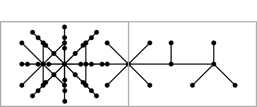
(b) A spider

(c) A radius-3 star

Figure 1: Illustration of (a) a caterpillar, (b) a spider (c) a radius-3 star.

1.3 Paper Structure

This paper is structured as follow: In Section 2, we prove that the differential coloring problem is NP-hard even for planar graphs (Theorem 2.1). In Section 3, we present tight upper bounds for regular caterpillars (Theorem 3.1) and spiders (Theorem 3.2). In Section 4, we present closed-form optimal labeling schemes (more intuitive than the known labeling scheme [19]) for regular caterpillars (Theorem 4.1) and for spiders with path lengths all even or all odd (Theorem 4.2). In Sections 5 and 6, we describe labeling algorithms which produce close-to-optimal labeling for caterpillars (Theorem 5.2) and biconnected triangle-free outer-planar graphs (Theorem 6.1), respectively. We conclude in Section 7 with open problems and future work.

2 Differential Coloring is NP-complete for Planar Graphs

In this section, we prove that the differential coloring problem is NP-hard even for planar graphs.

Theorem 2.1

Given a planar graph $G=(V,E)$ it is NP-hard to determine the differential chromatic number of $G$.

Proof

In order to prove that the problem is NP-hard, we employ a reduction from the well-known $3$-coloring problem, which is NP-complete for planar graphs  [7].

More precisely, let $G=(V,E)$ be an instance of the $3$-coloring problem mentioned above, i.e., graph $G$ is an $n$-vertex planar graph. In the following, we will construct a new planar graph $G^{\prime}$, so that $G^{\prime}$ has differential coloring of value at least $n$ if and only if $G$ is $3$-colorable.

Graph $G^{\prime}=(V^{\prime},E^{\prime})$ is constructed by attaching a path $v\rightarrow v_{1}\rightarrow v_{2}$ to each vertex $v\in V$ of $G$; see Figs. 2a and 2b. Hence, we can assume that $V^{\prime}=V\cup V_{1}\cup V_{2}$, where $V$ is the vertex set of $G$, $V_{1}$ contains the first vertices of each 2-length path and $V_{2}$ the second ones. Clearly, $G^{\prime}$ is planar on $3n$ vertices. Now, observe that if $G^{\prime}$ is $3$-colorable, then $G$ is $3$-colorable, as well. This is because $G$ is a subgraph of $G^{\prime}$. On the other hand, if $G$ is $3$-colorable, then $G^{\prime}$ is also $3$-colorable; for each vertex $v\in V$, simply color its neighbors $v_{1}$ and $v_{2}$ with two distinct colors different from the color of $v$. Next, we show that $G^{\prime}$ is $3$-colorable if and only if $G^{\prime}$ has differential coloring of value at least $n$.

(a) Instance $G=(V,E)$

(b) Graph $G^{\prime}=(V^{\prime},E^{\prime})$

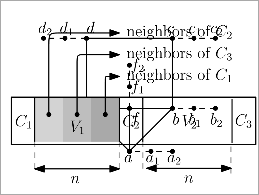
(c) Differential labeling

Figure 2: (a) An instance $G=(V,E)$ of the $3$-coloring problem; (b) An instance $G^{\prime}=(V^{\prime},E^{\prime})$ of the maximum differential coloring problem constructed based on graph $G$; (c) The differential labeling of $G^{\prime}$, in the case where $G$ is $3$-colorable.

First assume that $G^{\prime}$ has differential coloring of value at least $n$ and let $l:V^{\prime}\to\{1,2,\ldots,3n\}$ be the respective labeling. We proceed to color the vertices of $G^{\prime}$. Let $u\in V^{\prime}$ be a vertex of $G^{\prime}$. We assign a color $c(u)$ to $u$ as follows:

1. If $1\leq l(u)\leq n$, then $c(u)=1$

2. If $n+1\leq l(u)\leq 2n$, then $c(u)=2$

3. If $2n+1\leq l(u)\leq 3n$, then $c(u)=3$

Since labeling $l$ guarantees a differential coloring of value at least $n$, no two vertices with the same color are adjacent. Hence, coloring $c$ is a $3$-coloring for $G^{\prime}$.

Now, consider the case where $G^{\prime}$ is $3$-colorable. Let $C_{i}\subseteq V$ be the set of vertices of the input graph $G$ with color $i$, $i=1,2,3$. Obviously, $C_{1}\cup C_{2}\cup C_{3}=V$. We proceed to compute a labeling $l$ of the vertices of graph $G^{\prime}$ as follows (see Fig. 2c):

1. Vertices in $C_{1}$ are labeled with labels from $1$ to $|C_{1}|$.

2. Vertices in $C_{2}$ are labeled with labels from $n+|C_{1}|+1$ to $n+|C_{1}|+|C_{2}|$.

3. Vertices in $C_{3}$ are labeled with labels from $2n+|C_{1}|+|C_{2}|+1$ to $2n+|C_{1}|+|C_{2}|+|C_{3}|$.

4. For a vertex $v_{1}\in V_{1}$ neighboring to a vertex $v\in C_{1}$, $l(v_{1})=l(v)+n$.

5. For a vertex $v_{1}\in V_{1}$ neighboring to a vertex $v\in C_{2}$, $l(v_{1})=l(v)-n$.

6. For a vertex $v_{1}\in V_{1}$ neighboring to a vertex $v\in C_{3}$, $l(v_{1})=l(v)-2n$.

7. For a vertex $v_{2}\in V_{2}$ neighboring to a vertex $v_{1}\in V_{1}$, $l(v_{2})=l(v_{1})+n+|C_{2}|$.

From the above it follows that the label difference between (i) any two vertices in $G$, (ii) a vertex $v_{1}\in V_{1}$ and its neighbor $v\in V$, and, (iii) a vertex $v_{1}\in V_{1}$ and its neighbor $v_{2}\in V_{2}$ is at least $n$. So, $G^{\prime}$ has differential coloring of value at least $n$.

3 Upper Bounds for Regular Caterpillars and Spiders

In this section, we establish new upper bounds for $\mathrm{DC}(G)$, when $G$ is a regular caterpillar or a spider. Then, we show that the Miller-Pritikin labeling scheme is optimal for these classes of graphs.

Theorem 3.1

Let $G$ be a $\Delta$-regular caterpillar with $n$ vertices. If $G$ has an odd number of spine vertices, then $\mathrm{DC}(G)\leq\lceil\frac{n-\Delta}{2}\rceil$. Otherwise $\mathrm{DC}(G)\leq\lfloor\frac{n}{2}\rfloor$.

Proof

If $G$ has an even number of spine vertices, then by Property 1 it follows that $\mathrm{DC}(G)\leq\lfloor\frac{n}{2}\rfloor$. We will show that, when $G$ has an odd number of spine vertices, $\mathrm{DC}(G)\leq\lceil\frac{n-\Delta}{2}\rceil$. Let the number of spine vertices be $s=2k+1$, for some $k\geq 1$. Then, the total number of vertices of $G$ is $n=(2k+1)(\Delta+1)$. Note that $\lceil\frac{n-\Delta}{2}\rceil=1+k(\Delta+1)$. For a proof by contradiction assume that there exists a labeling of value $c^{*}=\lceil\frac{n-\Delta}{2}\rceil+1$.

Proof

Lemma 1

No spine vertex is labeled in the interval $[\lceil\frac{n-\Delta}{2}\rceil,\lceil\frac{n+\Delta}{2}\rceil]$

Proof

Assume to the contrary that $i\in[\lceil\frac{n-\Delta}{2}\rceil,\lceil\frac{n+\Delta}{2}\rceil]$ is a spine vertex label. Consider the labels that can be assigned to the $\Delta$ legs of $i$ (with a slight abuse of notation $i$ also refers to the vertex labeled $i$). To achieve value $c^{*}$ the label for a leg of $i$ can either lie in the interval $L=[1,i-(\lceil\frac{n-\Delta}{2}\rceil+1)]$ or in the interval $H=[i+\lceil\frac{n-\Delta}{2}\rceil+1,n]$. We consider three cases for the label of $i$.

1. $i\neq\lceil\frac{n-\Delta}{2}\rceil$ and $i\neq\lceil\frac{n+\Delta}{2}\rceil$. In this case, the total number of labels in $L$ and $H$ is:

   $$i-\left(\left\lceil\frac{n-\Delta}{2}\right\rceil+1\right)+n-\left(i+\left\lceil\frac{n-\Delta}{2}\right\rceil\right) = n-\left(2\left\lceil\frac{n-\Delta}{2}\right\rceil+1\right)$$

   $$= n-(2k(\Delta+1)+3)$$

   $$= n-(n+2-\Delta)~{}=~{}\Delta-2$$

2. $i=\lceil\frac{n-\Delta}{2}\rceil$. In this case, $L$ is empty and all leg labels lie in interval $H$. Hence, the total number of labels in $H$ is:

   $$n-\left(2\cdot\left\lceil\frac{n-\Delta}{2}\right\rceil\right) = n-(2\cdot((k\cdot(\Delta+1))+1)$$

   $$= ((2k+1)\cdot(\Delta+1))-(2\cdot((k\cdot(\Delta+1))+1))$$

   $$= \Delta-1$$

3. $i=\lceil\frac{n+\Delta}{2}\rceil$. In this case, $H$ is empty and all leg labels lie in interval $L$. Similarly to the previous case, the total number of labels in $L$ is: $i-\left(\left\lceil\frac{n-\Delta}{2}\right\rceil+1\right)=\Delta-1$

In all cases the labels for the legs of $i$ are insufficient. So, we have a contradiction.

Back to the theorem: By Lemma 1, it follows that labels of spine vertices either lie in the interval $L_{s}=[1,\lceil\frac{n-\Delta}{2}\rceil-1]$ or in the interval $H_{s}=[\lceil\frac{n+\Delta}{2}\rceil+1,n]$. Observe that the maximum difference between any two elements in the interval $L_{s}$ is $\lceil\frac{n-\Delta}{2}\rceil-2$. This suggests that in order to achieve differential coloring $c^{*}$, adjacent spine vertices cannot both be labeled from the interval $L_{s}$. Similarly, we can prove that adjacent spine vertices cannot both be labeled from the interval $H_{s}$, as the maximum difference between two elements in $H_{s}$ is $n-(\lceil\frac{n+\Delta}{2}\rceil+1)=n-(\lceil\frac{n-\Delta}{2}\rceil+\Delta+1)=n-(k\cdot(\Delta+1)+1+\Delta+1)=\lceil\frac{n-\Delta}{2}\rceil<c^{*}$.

From the above it follows that the labels for spine vertices must alternate between interval $L_{s}$ and $H_{s}$ such that for the labels of the $2k+1$ spine vertices, one of the intervals supplied $k+1$ labels and other interval supplied $k$ labels. Assume without loss of generality that $L_{s}$ supplies $k+1$ labels. In order to achieve differential coloring $c^{*}$, the $(k+1)\Delta$ legs of these spine vertices must all have labels in the interval $I=[\lceil\frac{n-\Delta}{2}\rceil+2,n]$. As $\Delta\geq 1$, interval $I\supseteq H_{s}$, and so $I$ must also contain the $k$ labels $H_{s}$ supplies for spine vertices. Thus, in total $I$ must contain at least $(k+1)\Delta+k$ labels. However, the size of the interval $I$ is:

$$1+n-(\lceil\frac{n-\Delta}{2}\rceil+2) = 1+((2k+1)\cdot(\Delta+1))-((k\cdot(\Delta+1))+1)-2$$

$$= k\cdot\Delta+k+\Delta-1$$

$$< (k+1)\Delta+k$$

So, we have a contradiction.

Corollary 1

The Miller-Pritikin labeling scheme is optimal for regular caterpillars.

Proof

Let $G$ be a regular caterpillar on $n$ vertices. First, consider the case where $G$ has an even number of spine vertices, say $s=2k$ for some $k\geq 1$. $G$ is a bipartite graph whose vertices form two disjoint sets $U$ and $V$, where $U$ consists of the $k$ odd spine vertices and the $k\Delta$ legs of the even spine vertices, and, $V$ consists of the $k$ even spine vertices and the $k\Delta$ legs of the odd spine vertices. So, $|U|=|V|=k+k\Delta=\frac{n}{2}$. Since the Miller-Pritikin labeling scheme yields a labeling with value equal to the size of the smaller vertex set, the labeling is optimal by Property 1.

Now, consider the case where $G$ has an odd number of spine vertices, say $s=2k+1$ for some $k\geq 1$. In this case, $U$ consists of the $k$ even spine vertices and the $(k+1)\Delta$ legs of the odd spine vertices, and, $V$ consists of $k+1$ odd spine vertices and the $k\Delta$ legs of the even spine vertices. So, $|U|=k+(k+1)\Delta$ and $|V|=k+1+k\Delta$, and $\min\{|U|,|V|\}=k+1+k\Delta=\lceil\frac{n-\Delta}{2}\rceil$. Thus, by Theorem 3.1 the Miller-Pritikin labeling scheme is optimal.

In the following, we present a tight upper bound for spider graphs. However, before presenting our labeling method, we make a few simple observations about spider graphs. Let $p$ be the number of paths connected to the center vertex $v_{c}$ in a spider graph $G$. Recall that by $N_{e}$, $N_{o}$ and $N_{l}$ we denote the number of even level, number of odd level and number of vertices in level $l$, respectively. Then, the number of vertices of $G$ is:

$$n=N_{e}+N_{o}+1$$ (1)

Each of the $p$ paths of $G$ starts with an odd level vertex and alternates between even and odd levels. It follows that on each path the number of odd level vertices is at most one more than the even level vertices. Summing over all $p$ paths we get:

$$N_{o}-N_{e}\leq p$$ (2)

Theorem 3.2

If $G$ is a spider graph with $N_{e}$ even level vertices, then $\mathrm{DC}(G)\leq N_{e}+1$.

Proof

For a proof by contradiction suppose that there exists a labeling of value $c^{*}=N_{e}+2$.

Proof

Lemma 2

The center vertex label is not in the interval $[N_{e}+1,N_{e}+p+1]$.

Proof

For the sake of contradiction, let $i\in[N_{e}+1,N_{e}+p+1]$ be the label of the center vertex and consider the labels that can be assigned to the $p$ vertices of level $1$. To achieve a differential coloring of value $c^{*}$, the labels of the level-$1$ vertices can either lie in the interval $L=[1,i-(N_{e}+2)]$ or in the interval $H=[N_{e}+2+i,n]$. We consider three cases for the values of $i$.

1. $i\neq N_{e}+1$ and $i\neq N_{e}+p+1$. Then, by Equations 1 and 2 the total number of labels in $L$ and $H$ is:

   $$i-N_{e}-2+n-(i+N_{e}+2)+1 = n-2N_{e}-3$$

   $$= N_{e}+N_{o}+1-2N_{e}-3\quad$$

   $$= N_{o}-N_{e}-2\leq p-2\quad$$

2. $i=N_{e}+1$. In this case, $L$ is empty and all labels of level-$1$ vertices lie in $H$. By Equations 1 and 2, the total number of labels in $H$ is:

   $$n-(i+N_{e}+2)+1 = n-(N_{e}+1+N_{e}+2)+1$$

   $$= N_{e}+N_{o}+1-(N_{e}+1+N_{e}+2)+1\quad$$

   $$= N_{o}-N_{e}-1\leq p-1\quad$$

3. $i=N_{e}+p+1$. In this case, $H$ is empty and all labels of level-$1$ vertices lie in $L$. Similarly to the previous case, the total number of labels in $L$ is: $i-N_{e}-2=N_{e}+p+1-N_{e}-2=p-1$

In all cases the number of labels is less than $p$, arriving to a contradiction and completing the proof of this lemma.

Back to the theorem: By Lemma 2, the center label either lies in interval $L_{c}=[1,N_{e}]$ or in interval $H_{c}=[N_{e}+p+2,n]$. Let us first assume that the center label lies in $L_{c}$ . In this case, the level-$1$ vertices should lie in the interval $I=[N_{e}+3,n]$. Note that in order to achieve a differential coloring of value $c^{*}=N_{e}+2$, adjacent vertices from neighboring levels $2j$ and $2j+1$ cannot both lie in the interval $[1,N_{e}+2]$. Also, $N_{2j+1}\leq N_{2j}$. It follows that the labels of at least $N_{2j+1}$ vertices lie in the interval $I$. So, interval $I$ must contain at least $N_{1}+N_{3}+\cdots=N_{o}$ elements. The contradiction follows from the size of the interval $I$, which is:

$$n-N_{e}-3+1 = N_{e}+N_{o}+1-N_{e}-3+1\quad$$

$$= N_{o}-1\quad$$

Now, assume that the center lies in the interval $H_{c}$. An analogous argument shows that the interval $I^{\prime}=[1,n-N_{e}-2]$ must contain at least $N_{o}$ elements which is more than the size of $I^{\prime}$, leading to a contradiction. As both cases result in contradictions, this completes the proof of Theorem 3.2.

Corollary 2

The Miller-Pritikin labeling scheme is optimal for spiders.

Proof

Let $G$ be a spider graph. Clearly, $G$ is a bipartite graph whose vertices form disjoint sets $U$ and $V$, where the even level vertices and the center vertex form $U$ and the odd level vertices form $V$. Labeling $G$ with the Miller-Pritikin scheme gives a differential coloring of value at least $m=\min\{|U|,|V|\}=\min\{N_{e}+1,N_{o}\}$.

We now prove that $m$ is optimal. We have that $N_{e}\leq N_{o}$. If $N_{e}=N_{o}$, then $m=N_{o}$. By Property 1, it follows that $\mathrm{DC}(G)$ is at most $\lfloor n/2\rfloor$, which by Equation 1 is at most $\lfloor(N_{o}+N_{e}+1)/2\rfloor=\lfloor(2N_{o}+1)/2\rfloor=N_{o}=m$. Now, assume that $N_{e}<N_{o}$. In this case, $m=N_{e}+1$ which is optimal by Theorem 3.2, completing the proof.

4 Optimal labeling for regular caterpillars and spiders with path lengths all even or all odd

In this section, we describe two optimal labeling schemes for regular caterpillars and spiders with path lengths all even or all odd, respectively. Note that by Corollaries 1 and 2 the Miller-Pritikin labeling scheme is also optimal for these classes of graphs. However, the labeling schemes that we present in this section are more intuitive, more structured and therefore of a simple nature compared to the Miller-Pritikin labeling scheme.

4.1 Optimal labeling for regular caterpillars

Let $G$ be an $n$-vertex regular caterpillar in which each spine vertex has $\Delta\geq 1$ legs. Let $s$ denote the number of spine vertices. Then, as $n=s\cdot(\Delta+1)$, we have $s=\frac{n}{\Delta+1}$.

It is always good to label all legs of a spine vertex $v$ from an interval of consecutive numbers, since the maximum difference between a spine vertex $v$ and its legs depends only on the difference between the label of $v$ and the highest or lowest label of the legs of $v$.

First, consider the case that there is an even number of spine vertices, say $s=2k$ for some $k\geq 1$. We label the spine vertices using the $k$ lowest and $k$ highest numbers in an alternating fashion. Starting with the leftmost spine vertex and moving to the right, we label the spine vertices as $1,n-k+1,2,n-k+2,\ldots$ and so on, ending at the rightmost spine vertices with numbers $k$ and $n$; see Fig. 3a. There are only two values for the differences between adjacent spine vertices, namely $n-k$ and $n-k-1$. As $\Delta\geq 1$, the difference is at least $n-k-1=2k\Delta+k-1\geq k(\Delta+1)=n/2$. We denote by $L_{s}$ the set of spine vertices with labels from $1$ to $k$, and, by $H_{s}$ the spine vertices with labels from $n-k+1$ to $n$.

Next, we split the middle range $[k+1,n-k]$ into two ranges $L_{\ell}=[k+1,\frac{n}{2}]$ and $H_{\ell}=[\frac{n}{2}+1,n-k]$. We label the legs of $L_{s}$ from the range $H_{\ell}$ and the legs of $H_{s}$ from the range $L_{\ell}$ as follows. For a spine vertex from $L_{s}$ with label $1\leq i\leq k$, we label its $\Delta$ legs with numbers from the interval $[\frac{n}{2}+((i-1)\cdot\Delta)+1,\frac{n}{2}+i\cdot\Delta]$. For a spine vertex from $H_{s}$ with label $j=n-k+i$ between $n-k+1$ and $n$, we label its $\Delta$ legs with numbers from the interval $[k+((i-1)\cdot\Delta)+1,k+i\cdot\Delta]$. It follows that the difference between a low spine vertex from $L_{s}$ and one of its legs is at least:

$$\frac{n}{2}+(i-1)\cdot\Delta+1-i = n/2+i(\Delta-1)-\Delta+1\quad$$

$$= n/2+(i-1)(\Delta-1)\quad$$

Then, it is not difficult to see that for $i=1$ this difference is minimized and equals to $\frac{n}{2}$. Analogously, the difference between a high spine vertex $j=n-k+i$ and one of its legs is at least:

$$j-(k+i\cdot\Delta) = n-k+i-k-i\cdot\Delta\quad$$

$$= n-2k+i(1-\Delta)\quad$$

In this case, the difference is minimized for the largest possible $i$, that is, $i=k$, and using the fact that $k=\frac{n}{2(\Delta+1)}$, the difference is again $\frac{n}{2}$. Hence, there exists a labeling for which the maximum difference is $\frac{n}{2}$.

(a) Even number of spine vertices.

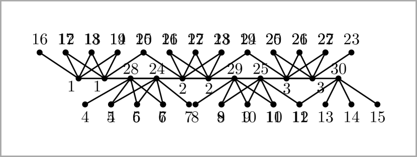
(b) Odd number of spine vertices.

Figure 3: Our optimal labeling for regular caterpillars.

Now, consider the case where the number of spine vertices is odd, say $s=2k+1$ for some $k\geq 1$; see Fig. 3b. We follow the scheme as above assigning the lowest $k+1$ numbers and the highest $k$ numbers in an alternating fashion to the spine vertices. The differences between adjacent spine vertices are $n-k$ and $n-k-1$ which is at least:

$$n-k-1 = 2k\Delta+\Delta+k\quad$$

$$\geq k\Delta+1+k\quad$$

$$\geq \lceil\frac{n-\Delta}{2}\rceil\quad$$

Let $L_{s}$ denote the spine vertices with labels $\leq k+1$ and $H_{s}$ be the spine vertices with labels $>n-k$. As before, we divide the middle range $[k+2,n-k]$ into two ranges $L_{\ell}=[k+2,\lceil\frac{n-\Delta}{2}\rceil]$ and $H_{\ell}=[\lceil\frac{n-\Delta}{2}\rceil+1,n-k]$ and label the legs of $H_{s}$ with number from $L_{\ell}$ and the legs of $L_{s}$ with numbers from $H_{\ell}$. For a spine vertex from $L_{s}$ with label $1\leq i\leq k+1$, we label its $\Delta$ legs with numbers from the interval $[\lceil\frac{n-\Delta}{2}\rceil+((i-1)\cdot\Delta)+1,\lceil\frac{n-\Delta}{2}\rceil+i\cdot\Delta]$. For a spine vertex from $H_{s}$ with label $j=n-k+i$ between $n-k+1$ and $n$, we label its $\Delta$ legs with numbers from the interval $[k+((i-1)\cdot\Delta)+2,k+i\cdot\Delta+1]$.

The difference between a low spine vertex $i$ and its legs is at least $\lceil\frac{n-\Delta}{2}\rceil+((i-1)\cdot\Delta)+1-i$ which is minimal for $i=1$, namely $\lceil\frac{n-\Delta}{2}\rceil$ as above. The difference between a high spine vertex $j=n-k+i$ and its legs is at least:

$$j-(k+i\cdot\Delta+1) = n-k+i-(k+i\cdot\Delta+1)\quad$$

$$\geq n-2k+i(1-\Delta)-1\quad$$

In this case, the difference is minimized for $i$ as large as possible, that is, $i=k$. Using the fact that $k=\frac{n-(\Delta+1)}{2(\Delta+1)}$ and as $\Delta\geq 1$, we have that the difference for $i=k$ is:

$$n-2k+k(1-\Delta)-1 = n-k-k\Delta-1=n-k(1+\Delta)-1\quad$$

$$\geq \lceil\frac{n-\Delta}{2}\rceil\quad$$

From the above, it follows that for a regular caterpillar with even number of spine vertices our labeling method achieves difference $\frac{n}{2}$ and for odd number of spine vertices it achieves difference $\lceil\frac{n-\Delta}{2}\rceil$. Both of these are optimal by Theorem 3.1. This is summarized in the following theorem.

Theorem 4.1

Let $G$ be a regular caterpillar with $n$ vertices. There exists an optimal labeling of $G$ with value $\frac{n}{2}$ when $G$ has an even number of spine vertices, and with value $\lceil\frac{n-\Delta}{2}\rceil$ otherwise.

4.2 Labeling spiders with path lengths all even or all odd

Let $G$ be a $n$-vertex spider consisting of $p$ paths. Recall that by $N_{l}$ we denote the number of vertices at level $l$. For each $q\in[1,N_{l}]$, let $v_{l,q}$ be the level-$l$ vertex that belongs to the $q$-th path out of the paths containing level-$l$ vertices.

Theorem 4.2

Let $G$ be a spider graph with $N_{e}$ even level vertices. If the paths of $G$ are all of odd length or all of even length, there exist optimal labeling for $G$ with value $N_{e}+1$ and $N_{e}$, respectively.

Proof

We consider the cases where all $p$ paths of $G$ are either of odd length or of even length separately. We first consider the case where all $p$ paths have even length; see Fig. 4a. We label the center vertex as $1$. The $N_{e}$ even level vertices will be labeled with numbers from interval $I_{e}=[2,N_{e}+1]$ in increasing order of levels, i.e., starting with the level-$2$ vertices, followed by level-$4$ vertices, etc. The $N_{o}$ odd level vertices will be labeled with numbers from the interval $I_{o}=[N_{e}+2,n]$ in the same way, i.e., starting with the level-$1$ vertices, followed by the level-$3$ vertices, etc. For each level, we order the vertices in decreasing order of the lengths of the paths they belong to. More specifically, we initially order the $p$ paths in decreasing order of their lengths. Then, the exact label of each vertex is determined as follow; see Fig. 5a:

(a) All paths of even lengths.

(b) All paths of odd lengths.

Figure 4: Special cases of spider graphs where our labeling is optimal.

1. A vertex $v_{l,q}$ belonging to an odd level $l=2i+1$, $i\geq 1$ is labeled as $N_{e}+1+\sum_{k=0}^{i-1}N_{2k+1}+q$.

2. A vertex $v_{l,q}$ belonging to an even level $l=2i$, $i\geq 1$ is labeled as $1+\sum_{k=1}^{i-1}N_{2k}+q$.

We now show that the above labeling has maximum differential value $N_{e}$. First, consider the difference between the center and a level-$1$ vertex $v_{1,q}$. The difference is $N_{e}+1+q-1$. As $q\in[1,p]$, this is at least $N_{e}+1\geq N_{e}$.

Now, consider the difference between a vertex of level $l=2i$ and a vertex of level $l+1=2i+1$, for some $i\geq 1$. Since $N_{2k+1}\geq N_{2k+2}$, the difference is:

$$v_{l+1,q}-v_{l,q} = N_{e}+1+\sum_{k=0}^{i-1}N_{2k+1}+q-(1+\sum_{k=1}^{i-1}N_{2k}+q)\quad$$

$$= n-k(1+\Delta)-1\quad$$

$$= N_{e}+N_{2(i-1)+1}+\sum_{k=0}^{i-2}(N_{2k+1}-N_{2k+2})\quad$$

$$\geq N_{e}+N_{2(i-1)+1}\geq N_{e}\quad$$

Now, consider the difference between a vertex $v_{l,q}$ at level $l=2i$ and a vertex $v_{l-1,q}$ on the same path. In this case and since $N_{2k+1}\geq N_{2k+2}$, the difference is:

$$v_{l-1,q}-v_{l,q} = N_{e}+1+\sum_{k=0}^{i-2}N_{2k+1}+q-(1+\sum_{k=1}^{i-1}N_{2k}+q)\quad$$

$$= N_{e}+\sum_{k=0}^{i-2}(N_{2k+1}-N_{2k+2})\geq N_{e}\quad$$

From the above, it follows that our labeling for the case, where all $p$ paths have even length, has maximum differential value $N_{e}$, as desired. Since all the paths have even length $N_{e}=N_{o}=\lceil\frac{n}{2}\rceil$.

We now consider the case where all of the $p$ paths have odd length; see Fig. 4b. Let $k$ be the length of the longest path. Since all paths have odd length, we have $N_{2i}=N_{2i+1}\forall i\in[1,\lfloor\frac{k}{2}\rfloor]$. Also, $N_{o}-N_{e}=N_{1}+\sum_{i=1}^{\lfloor\frac{k}{2}\rfloor}(N_{2i+1}-N_{2i})=p$, and, $n=N_{o}+N_{e}+1=2N_{e}+p+1$. So, $n$ and $p$ have different parity. On the other hand, $\lceil\frac{n-p}{2}\rceil=N_{e}+1$. We label the center vertex as $\lceil\frac{n}{2}\rceil$. We next order the paths as $P_{\lfloor\frac{p}{2}+1\rfloor},P_{1},P_{\lfloor\frac{p}{2}+2\rfloor},P_{2}\dots$ in the decreasing order of their lengths. Then, the exact label of each vertex is determined as follow; see Fig. 5b:

1. A vertex $v_{l,q}$ belonging to an odd level $l=2i-1$ and $q\leq\lfloor\frac{p}{2}\rfloor$ is labeled as $\sum_{m=1}^{i-1}\lfloor\frac{N_{2m-1}}{2}\rfloor+q$.

2. A vertex $v_{l,q^{\prime}}$ belonging to an odd level $l=2i-1$ and $q^{\prime}>\lfloor\frac{p}{2}\rfloor$, $q^{\prime}=q+\lfloor\frac{p}{2}\rfloor$ is labeled as $n-(\sum_{m=1}^{i}\lceil\frac{N_{2m-1}}{2}\rceil)+q$.

3. A vertex $v_{l,q}$ belonging to an even level $l=2i$ and $q\leq\lfloor\frac{p}{2}\rfloor$ is labeled as $\lceil\frac{n}{2}\rceil+\sum_{m=1}^{i-1}\lfloor\frac{N_{2m}}{2}\rfloor+q$.

4. A vertex $v_{l,q^{\prime}}$ belonging to an even level $l=2i$ and $q^{\prime}>\lfloor\frac{p}{2}\rfloor$, $q^{\prime}=q+\lfloor\frac{p}{2}\rfloor$ is labeled as $\lceil\frac{n}{2}\rceil-(\sum_{m=1}^{i}\lceil\frac{N_{2m}}{2}\rceil)+q-1$.

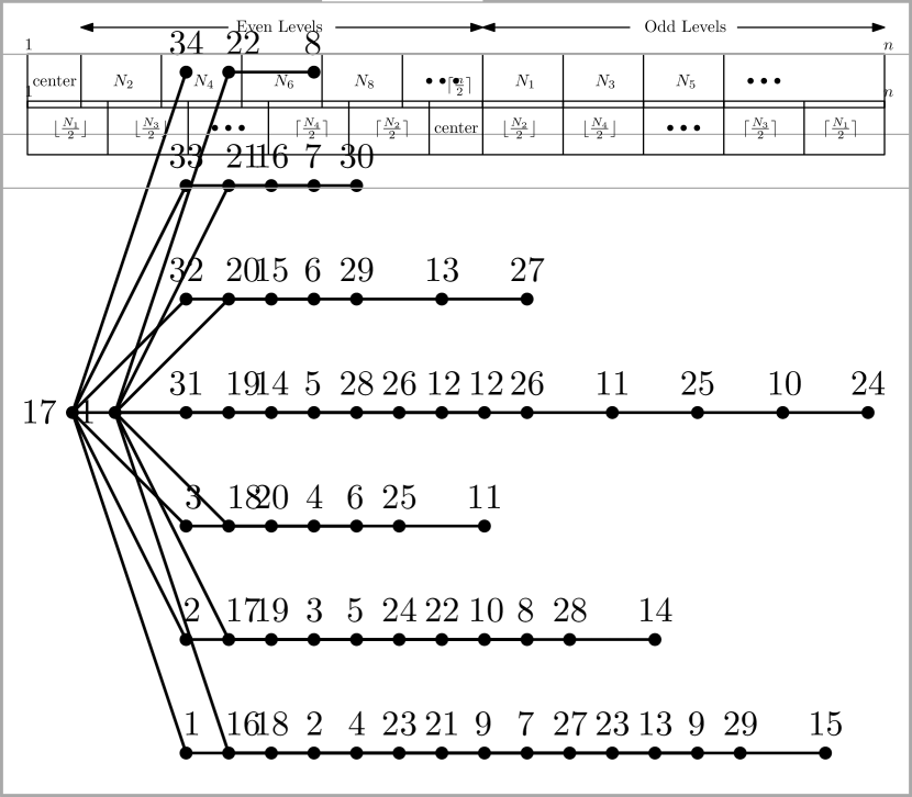
(a) The labeling scheme for spiders with all paths of even length.

(b) The labeling scheme for spiders with all paths of odd length.

Figure 5: The two cases of our spider labeling scheme.

We now show that the above labeling has maximum differential value $N_{e}+1$. First, consider the difference between the center and a level-$1$ vertex $v_{1,q}$. When $q\leq\lfloor\frac{p}{2}\rfloor$, the difference is $\lceil\frac{n}{2}\rceil-q$, which is at least $\lceil\frac{n}{2}\rceil-\lfloor\frac{p}{2}\rfloor=\lceil\frac{n-p}{2}\rceil$ . When $q^{\prime}>\lfloor\frac{p}{2}\rfloor,q^{\prime}=q+\lfloor\frac{p}{2}\rfloor$, the difference is $n-\lceil\frac{N_{1}}{2}\rceil+q-\lceil\frac{n}{2}\rceil$, which is at least $n-\lceil\frac{p}{2}\rceil+1-\lceil\frac{n}{2}\rceil=\lfloor\frac{n}{2}\rfloor-\lceil\frac{p}{2}\rceil+1=\lceil\frac{n-p}{2}\rceil$.

Now, consider the difference between the labels of vertices in level $l=2i$ and level $l-1=2i-1$. Since for every $m$ it holds that $\lfloor\frac{N_{2m}}{2}\rfloor\geq\lfloor\frac{N_{2m-1}}{2}\rfloor$, for $q\leq\lfloor\frac{p}{2}\rfloor$ the difference is:

$$v_{l-1,q}-v_{l,q} = \lceil\frac{n}{2}\rceil+\sum_{m=1}^{i-1}\lfloor\frac{N_{2m}}{2}\rfloor+q-(\sum_{m=1}^{i-1}\lfloor\frac{N_{2m-1}}{2}\rfloor)+q)\quad$$

$$= N_{e}+\sum_{k=0}^{i-2}(N_{2k+1}-N_{2k+2})\quad$$

$$\geq \lceil\frac{n}{2}\rceil\quad$$

Analogously, for $q^{\prime}=q+\lfloor\frac{p}{2}\rfloor$ and $q^{\prime}>\lfloor\frac{p}{2}\rfloor$ the difference is:

$$v_{l-1,q^{\prime}}-v_{l,q^{\prime}} = n-(\sum_{m=1}^{i}\lceil\frac{N_{2m-1}}{2}\rceil)+q-(\lceil\frac{n}{2}\rceil-(\sum_{m=1}^{i}\lceil\frac{N_{2k}}{2}\rceil)+q-1)\quad$$

$$\geq \lfloor\frac{n}{2}\rfloor+1\quad$$

Since $\lfloor\frac{n}{2}\rfloor+1\geq\lceil\frac{n}{2}\rceil$, in both cases the difference is at least $\lceil\frac{n}{2}\rceil$. Now, consider the difference between a vertex $v_{l,q}$ at level $l=2i$ and a vertex $v_{l+1,q}$ on the same path. For $q\leq\lfloor\frac{p}{2}\rfloor$ the difference is:

$$v_{l+1,q}-v_{l,q} = \lceil\frac{n}{2}\rceil+\sum_{m=1}^{i-1}\lfloor\frac{N_{2m}}{2}\rfloor+q-(\sum_{m=1}^{i}\lfloor\frac{N_{2m-1}}{2}\rfloor)+q)\quad$$

$$\geq \lceil\frac{n}{2}\rceil-\lfloor\frac{N_{2i-1}}{2}\rfloor\quad$$

$$\geq \lceil\frac{n}{2}\rceil-\lfloor\frac{p}{2}\rfloor=\lceil\frac{n-p}{2}\rceil\quad$$

Analogously, for $q^{\prime}=q+\lfloor\frac{p}{2}\rfloor$ and $q^{\prime}>\lfloor\frac{p}{2}\rfloor$ the difference is:

$$v_{l-1,q^{\prime}}-v_{l,q^{\prime}} = (n-(\sum_{m=1}^{i+1}\lceil\frac{N_{2m-1}}{2}\rceil)+q)-(\lceil\frac{n}{2}\rceil-(\sum_{m=1}^{i}\lceil\frac{N_{2m}}{2}\rceil)+q-1)\quad$$

$$= \lfloor\frac{n}{2}\rfloor+1-\lceil\frac{N_{2i+1}}{2}\rceil\quad$$

$$\geq \lfloor\frac{n}{2}\rfloor+1-\lceil\frac{p}{2}\rceil=\lceil\frac{n-p}{2}\rceil$$

We now argue that we achieve an optimal labeling for $G$ if all paths are of even length. Recall that in this case our labeling scheme achieves a maximum differential value of $N_{e}$. As all paths have even lengths, $N_{e}=N_{o}$. Thus, $n=N_{e}+N_{o}+1=2N_{e}+1$. By Property 1, it follows that $\mathrm{DC}(G)\leq\lceil n/2\rceil=\lceil(2N_{e}+1)\rceil=N_{e}$. In the case where $G$ is a spider with all paths of odd length, our labeling achieves a maximum differential value of $N_{e}+1$, which is optimal by Theorem 3.2. This completes the proof of Theorem 4.2.

Now, recall that a $k$-radius star $G$ is a spider where all paths have length exactly $k$. As $k$ is either an even or an odd number, either all paths of $G$ are of even length or all paths are of odd length. Thus, our labeling scheme is optimal for $k$-radius star graphs. Hence, we can state the following as a corollary of Theorem 4.2.

Corollary 3

There exists a linear-time algorithm that computes an optimal labeling for all radius-$k$ star graphs.

5 Labeling General Caterpillars

We start with a labeling scheme for the more intuitive –but slightly restricted– case, where $G$ is a caterpillar and each spine vertex has at least one leg. Then, we adapt the proposed scheme to general caterpillars.

5.1 Labeling for caterpillars with no missing legs

We describe a labeling algorithm for $G$ that achieves differential value at least $n/2-\Delta-1$, comprising of two phases; the marking phase and the labeling phase. The marking phase places the vertices of $G$ into one of the following sets: $L_{s}$, $H_{s}$, $M$, $L_{\ell}$, $H_{\ell}$, $L_{M_{\ell}}$ and $H_{M_{\ell}}$; see Fig. 6. The labeling phase assigns actual values to vertices of $G$.

Figure 6: Allocation of labels to the vertices of a caterpillar graph; legs of $L_{s}$ are labeled with numbers from the interval $H_{\ell}$ and legs of $H_{s}$ are labeled with numbers values from the interval $L_{\ell}$.

Theorem 5.1

Let $G$ be a caterpillar with $n$ vertices in which each spine vertex has at least one leg. There exists a labeling of $G$ with differential coloring value at least $\lceil\frac{n}{2}\rceil-\Delta-1$.

Proof

As already stated, our labeling algorithm is comprising of two phases; the marking phase and the labeling phase.

Marking: Vertices in $L_{s},H_{s},M$ are spine vertices and those in $L_{\ell}$, $H_{\ell}$, $L_{M_{\ell}}\cup H_{M_{\ell}}$ are the legs of spine vertices in $H_{s}$, $L_{s}$ and $M$, respectively. More precisely, the vertex in $M$ is labeled as $\lceil n/2\rceil$, the vertices in $L_{s},L_{\ell},L_{M_{\ell}}$ are labeled with low values $<\lceil n/2\rceil$, and those in $H_{s},H_{\ell},H_{M_{\ell}}$ are labeled high values $>\lceil n/2\rceil$.

Start by placing all odd-numbered spine vertices in set $L_{s}$ and all even-numbered ones in $H_{s}$, assuming that the spine vertices are numbered according to their position in the spine path. The legs of a spine vertex $v\in L_{s}$ are placed into $H_{\ell}$ and the legs of a spine vertex $v\in H_{s}$ into $L_{\ell}$. Now, select one vertex to place into set $M$ by traversing the spine vertices $S=L_{s}\cup H_{s}$ from right to left. At each vertex $v_{i}\in S$ we temporarily ignore $v_{i}$ and its legs from their current sets and check if the following balance condition holds:

$$|L_{s}|+|L_{\ell}|<n/2 |H_{s}|+|H_{\ell}|\leq n/2$$ and (3)

Intuitively, when the balance condition holds the number of vertices which we will label with low and high values are both less than $n/2$. If the balance condition holds at $v_{i}\in S$, we place $v_{i}$ in set $M$. Otherwise, we flip $v_{i}$ and its legs as follows: if $v_{i}$ is in set $L_{s}$, then we move it into set $H_{s}$ and move its legs into $L_{\ell}$; else if $v_{i}$ is in set $H_{s}$, then we move it into set $L_{s}$ and its legs into $H_{\ell}$.

We claim that the process always stops with a configuration where the balance condition holds. Suppose without loss of generality that initially $|L_{s}|+|L_{\ell}|<n/2$ but $|H_{s}|+|H_{\ell}|>n/2$. As vertices and its legs are flipped during the traversal, if the balance condition is not met in the end, then we must have $|L_{s}|+|L_{\ell}|>n/2$ and $|H_{s}|+|H_{\ell}|<n/2$. Hence, at some point in the traversal, we switch from $|L_{s}|+|L_{\ell}|<n/2$ to $|L_{s}|+|L_{\ell}|>n/2$, when we flip some vertex $v_{i}$ and its legs. Ignoring this vertex $v_{i}$ and its legs ensures that $|L_{s}|+|L_{\ell}|<n/2$. Thus, we can place vertex $v_{i}$ into $M$ and stop.

Let $v_{m}$ be the vertex placed into $M$. Now, we partition the at most $\Delta$ legs of $v_{m}$ into sets $L_{M_{\ell}}$ and $H_{M_{\ell}}$, such that the total low and high values are:

Low values: $$|L_{s}|+|L_{\ell}|+|L_{M_{\ell}}|+|M|=\lceil n/2\rceil$$ (4)

High values: $$|H_{s}|+|H_{\ell}|+|H_{M_{\ell}}|=\lfloor n/2\rfloor$$ (5)

Labeling: Label $v_{m}$ as $\lceil n/2\rceil$. Then, label the legs of $v_{m}$ in $L_{M_{\ell}}$ with values from the interval $[1,|L_{M_{\ell}}|]$ and its legs in $H_{M_{\ell}}$ with values from the interval $[n-|H_{M_{\ell}}|+1,n]$. As $v_{m}$ has at most $\Delta$ legs, the minimum difference value between $v_{m}$ and its legs is:

$$\min\{\lceil n/2\rceil-|L_{M_{\ell}}|,\lceil n/2\rceil-|H_{M_{\ell}}|\}\geq n/2-\Delta$$ (6)

For the spine vertices $S=L_{s}\cup H_{s}$, label the vertices of $L_{s}$ with numbers from the interval $I(L_{s})=[|L_{M_{\ell}}|+1,|L_{M_{\ell}}|+|L_{s}|]$ and the vertices of $H_{s}$ with numbers the interval $I(H_{s})=[n-|H_{M_{\ell}}|-|H_{s}|+1,n-|H_{M_{\ell}}|]$. Start by labeling the spine neighbors of $v_{m}$. By the balancing procedure, $v_{m}$ has at most one spine neighbor from $L_{s}$ and one spine neighbor from $H_{s}$. The neighbor from $L_{s}$ (if it exists) is labeled as $|L_{M_{\ell}}|+1$ and the neighbor from $H_{s}$ (if it exists) is labeled as $n-|H_{M_{\ell}}|$. The difference between $v_{m}$ and its spine neighbors is:

$$\min\{\lceil n/2\rceil-|L_{M_{\ell}}|,n-|H_{M_{\ell}}|-\lceil n/2\rceil\}\geq n/2-\Delta-1$$ (7)

The remaining spine vertices of $L_{s}$ are labeled with remaining numbers of $I(L_{s})$ in increasing order. Start with the first vertex in $L_{s}$ which is left of $v_{m}$, then move leftward labeling vertices from $L_{s}$ until reaching the leftmost vertex in $L_{s}$. Now, proceed to the rightmost vertex in $L_{s}$ and move leftward again until $v_{m}$ is reached. Label the spine vertices of $H_{s}$ with the remaining numbers from the interval $I(H_{s})$ in exactly the same way, i.e., in an increasing fashion starting from the vertex in $H_{s}$ to the left of $v_{m}$ and moving leftward. As we always increment the spine vertices by one, the difference between a spine vertex and its adjacent spine vertices is either:

$$|L_{s}|+|L_{\ell}|+|M|+|H_{\ell}|\mbox{ or }$$

$$|L_{s}|+|L_{\ell}|+|M|+|H_{\ell}|-1$$ (8)

In both cases, the difference is at least $|L_{s}|+|L_{\ell}|+|M|-1$, which by Equation 4 is at least $n/2-|L_{M_{\ell}}|-1\geq n/2-\Delta-1$.

We now describe how the leg vertices are labeled. The labels of $L_{\ell}$ come from interval $I(L_{\ell})=[|L_{M_{\ell}}|+|L_{s}|+1,\lceil n/2\rceil-1]$. The labels of $H_{\ell}$ come from the interval $I(H_{\ell})=[\lceil n/2\rceil+1,\lceil n/2\rceil+|H_{\ell}|]$. The values of $I(H_{\ell})$ are assigned in increasing order starting with the legs of the spine vertex of $L_{s}$ with the lowest value. Thus, we first label the legs of the spine vertex labeled $|L_{M_{\ell}}|+1$, then the legs of $|L_{M_{\ell}}|+2$, and so on until $|L_{M_{\ell}}|+|L_{s}|$. Assign the values of $I(L_{\ell})$ in decreasing order starting with the spine vertex of $H_{s}$ with the highest label. Thus, the legs of $n-|H_{M_{\ell}}|$ are labeled first, then the legs of $n-|H_{M_{\ell}}|-1$ and so on until $n-|H_{M_{\ell}}|-|H_{s}|+1$.

As all spine vertices have at least one leg, the difference between the $j$-th lowest spine vertex of $L_{s}$ and one of its legs is at least the value given by Equation 9 (same for $H_{s}$):

$$|L_{s}|-j+|L_{\ell}|+|M|+j \geq \lceil n/2\rceil-|L_{M_{\ell}}|-1~{}\mbox{ by Equation~{}\ref{eq:totallow}}$$

$$|H_{s}|-j+|H_{\ell}|+|M|+j \geq \lceil n/2\rceil-|H_{M_{\ell}}|-1~{}\mbox{ by Equation~{}\ref{eq:totalhigh}}$$ (9)

As $|L_{M_{\ell}}|$ and $|H_{M_{\ell}}|$ are both $\leq\Delta$, the differences are at least $n/2-\Delta-1$.

5.2 Extending to general caterpillars

We extend the labeling scheme to general caterpillars to achieve differential value at least $n/2-\Delta-2$. The main idea is to consider spine vertices with no legs as pseudo-legs of their neighbors, thus transforming a general caterpillar into a caterpillar where all but one spine vertex have at least one leg or pseudo-leg; see Fig. 7. Observe that the rightmost spine vertex has at least one leg as otherwise it is a leg of the spine vertex to its left.

Theorem 5.2

Let $G$ be a caterpillar with $n$ vertices. There exists a labeling of $G$ with differential coloring value at least $\lceil\frac{n}{2}\rceil-\Delta-2$.

Proof

Again, our labeling algorithm is comprising of two phases; the marking phase and the labeling phase.

Marking: Select a vertex $v_{m}$ for set $M$ as before. Then, traverse the spine from left to right to determine which vertices are pseudo-legs. Let $v$ be the current spine vertex and $v^{\prime}$ be the spine vertex to the right of $v$. If $v\neq v_{m}$ and $v$ currently has no legs or pseudo-legs, then first assign $v$ to be a pseudo-leg of $v^{\prime}$ and move $v$ into the corresponding set as follows: if $v^{\prime}\in L_{s}$, then move $v$ into set $H_{\ell}$, if $v^{\prime}\in H_{s}$, then move $v$ into set $L_{\ell}$, and if $v^{\prime}\in M$, then keep $v$ in its current set. Observe that in the first case vertex $v$ moves from set $H_{s}$ into set $H_{\ell}$, and in the second it moves from set $L_{s}$ into set $L_{\ell}$. Thus, the number of low and high values to be assigned both remain $<n/2$ and the balance condition in Equation 3 is still satisfied.

Now, let $v_{m}^{\prime}$ be the right neighbor of $v_{m}$ on the spine. If $v_{m}^{\prime}$ is currently a pseudo-leg, then reassign $v_{m}^{\prime}$ to be a pseudo-leg of $v_{m}$, and if $v_{m}^{\prime}\in L_{\ell}$, then move $v_{m}^{\prime}$ into $L_{s}$ and if $v_{m}^{\prime}\in H_{\ell}$, then move it into $H_{s}$. Note that the balance condition in Equation 3 is maintained. However, as we reassigned $v_{m}^{\prime}$ to be a pseudo-leg of $v_{m}$, this may leave one vertex, namely the spine vertex to the right of $v_{m}^{\prime}$ with no legs. Finally, partition the real legs of $v_{m}$ into sets $L_{M_{\ell}}$ and $H_{M_{\ell}}$ as before.

Figure 7: Labeling of a general caterpillar, where the spine vertices drawn as squares correspond to pseudo-legs.

Labeling: Label $v_{m}$ as $\lceil n/2\rceil$. Then, label $v_{m}$’s real legs and its neighboring vertices on the spine also as before. Note that no the two neighboring spine vertices of $v_{m}$ may be pseudo-legs of $v_{m}$. Still, one of them is in the set $L_{s}$ and the other is in the set $H_{s}$, and we label these as $|L_{M_{\ell}}|+1$ and $n-|H_{M_{\ell}}|$, respectively. Equations 6 and 7 still apply, so the differential value for $v_{m}$ is at least $n/2-\Delta-1$.

We label the remaining spine vertices from $S=L_{s}\cup H_{s}$ and their legs and pseudo-legs $L_{\ell}\cup H_{\ell}$ as before. We show that the difference between adjacent vertices is at least $n/2-\Delta-2$. First consider two adjacent vertices from $S$. Their difference is still given by Equation 8 and is at least $|L_{s}|+|L_{\ell}|+|M|-1$. By Equation 4 this is at least $n/2-|L_{M_{\ell}}|-1$, and as $|L_{M_{\ell}}|\leq\Delta$, the difference is $\geq n/2-\Delta-1$.

Next, consider a vertex $v\in S$ and its legs (including its pseudo-leg). We modify Equation 9 to take into account that at most one spine vertex may have no legs. The difference between the $j$-th lowest spine vertex of $L_{s}$ and one of its legs and the $j$-th lowest spine vertex of $H_{s}$ and one of its legs is at least:

$$|L_{s}|-j+|L_{\ell}|+|M|+(j-1) \geq \lceil n/2\rceil-|L_{M_{\ell}}|-1~{}\mbox{ by Equation~{}\ref{eq:totallow}}$$

$$|H_{s}|-j+|H_{\ell}|+|M|+(j-1) \geq \lceil n/2\rceil-|H_{M_{\ell}}|-1~{}\mbox{ by Equation~{}\ref{eq:totalhigh}}$$

As $|L_{M_{\ell}}|$ and $|H_{M_{\ell}}|$ are both $\leq\Delta$, the difference is at least $n/2-\Delta-1$.

Finally, consider a vertex $v\in S$ which is adjacent to $v_{p}$, where $v_{p}$ is a pseudo-leg of $v^{\prime}\in S$, $v^{\prime}\neq v$. Each vertex $v\in S$ may be adjacent to at most one such $v_{p}$. As $v^{\prime}$ may have $v_{p}$ as its only leg and as there is at most one spine vertex with no legs, the difference depending on the label of $v$ is at least:

$$|L_{s}|-j+|L_{\ell}|+|M|+(j-2) \geq \lceil n/2\rceil-|L_{M_{\ell}}|-2~{}\mbox{ by Equation~{}\ref{eq:totallow}}$$

$$|H_{s}|-j+|H_{\ell}|+|M|+(j-2) \geq \lceil n/2\rceil-|H_{M_{\ell}}|-2~{}\mbox{ by Equation~{}\ref{eq:totalhigh}}$$

As $|L_{M_{\ell}}|$ and $|H_{M_{\ell}}|$ are $\leq\Delta$, the difference is $\geq n/2-\Delta-2$, which completes the proof of Theorem 5.2.

5.3 Comparison with the Miller-Pritikin scheme

Consider a non-regular caterpillar with $s=2k+1$ spine vertices, where the $k+1$ odd spine vertices have one leg each and the $k$ even spine vertices have $\Delta$ legs each. This forms a bipartite graph with disjoint vertex sets $U$ and $V$, where the $k+1$ odd spine vertices and the $k\Delta$ legs of even spine vertices form the set $U$, and the rest of the vertices form set $V$. The Miller-Pritikin labeling achieves differential value equal to the size of the smaller vertex set, i.e., $\min\{|U|,|V|\}=2k+1$. On the same graph, our labeling scheme achieves differential value at least $n/2-\Delta-1=\frac{2k+1+(k+1)+(\Delta k)}{2}-\Delta-1\geq\frac{k}{2}(\Delta-1)$. Let $\Delta=\Omega(n)$ and $k=O(1)$. Then, the Miller-Pritikin scheme achieves differential value $O(1)$, while our labeling scheme achieves differential value $O(n)$, making it potentially worse than ours by a factor of $\Omega(n)$.

(a)

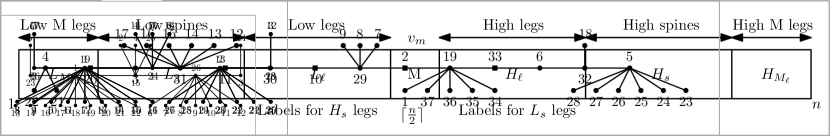
(b)

(c)

Figure 8: Three different labeling of a caterpillar graph. (a) The labeling given by Theorem 5.2 achieves differential value $18-13=5$. (b) The Miller-Pritikin labeling achieves differential value $8-1=7$. (c) A manually generated labeling achieving differential value $25-15=10$.

Note that there are graphs for which the Miller-Pritikin scheme achieves differential value better than the one that our labeling scheme achieves. Fig. 8a gives an example of a caterpillar labeled in three different ways; by our labeling scheme (of Theorem 5.2), by the Miller-Pritikin labeling scheme and by a manually generated one. Observe that our labeling achieves the lowest differential value; the Miller-Pritikin labeling is only slightly better, while the manually generated labeling is twice as good as our labeling.

6 Differential Coloring of biconnected triangle-free outer-planar graphs

We first show how to obtain a $3$-equitable coloring (coloring with $3$ colors, in which the number of vertices of each color may differ by at most one) of a biconnected triangle-free outer-planar graph $G$. Then, we use this coloring to obtain a differential coloring of $G$ with value $\geq\frac{n}{3}-1$. The existence of $3$-equitable colorability of biconnected triangle-free outer-planar graphs is known [28], but not all $3$-equitable colorings can be converted to differential colorings with the desired bound. Unlike the existential proof in [28], our proof is constructive and our algorithm also guarantees that the computed coloring can be appropriately converted to a differential coloring of $G$ with value $\geq\frac{n}{3}-1$.

Lemma 3

Given a biconnected triangle-free outer-planar graph $G$ on $n$ vertices, there is an $O(n)$-time algorithm that computes a $3$-equitable coloring of $G$.

Proof

Our algorithm is recursive. Consider an arbitrary edge $(u,v)$ of $G$ that does not belong to its external face and let $f$ and $g$ be the faces to its left and the right side, respectively, as we move along $(u,v)$ from vertex $u$ to vertex $v$. Then, $f$ and $g$ correspond to two vertices, $v_{f}$ and $v_{g}$, of the weak dual of $G$ and $(v_{f},v_{g})$ is an edge in the weak dual; see Fig. 9a. The weak dual is the subgraph of the dual graph whose vertices correspond only to the bounded faces of the primal graph. Since the weak dual of a biconnected outer-planar graph is a tree (not a forest), the removal of edge $(v_{f},v_{g})$ results in two trees $T_{f}$ and $T_{g}$ rooted at vertices $v_{f}$ and $v_{g}$ of the dual of $G$, respectively. For the recursive step of our algorithm, we assume that we have already computed a $3$-equitable coloring for the subgraph, say $G_{f}$, of $G$ induced by $T_{f}$.

(a)

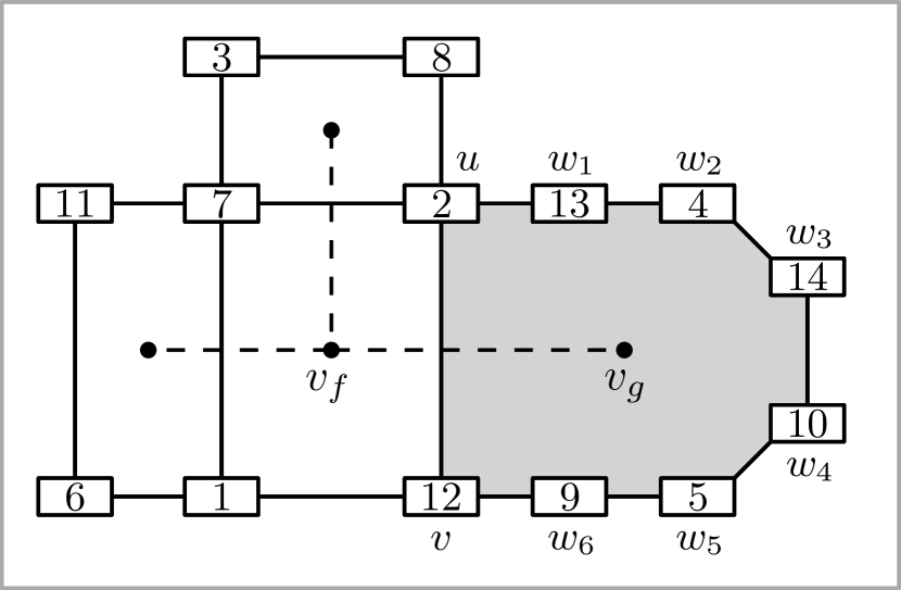
(b)

Figure 9: (a) A $3$-equitable coloring of a biconnected triangle-free outer-planar graph. (b) The corresponding differential labeling of value $14-10=4$.

We recursively compute a $3$-equitable coloring for the subgraph, say $G_{g}$, of $G$ induced by $T_{g}$, so that the overall coloring is a $3$-equitable coloring for $G$. Assume that $g=u,w_{1},w_{2},\ldots,w_{p},v$. Since $(u,v)$ is an edge of $G_{f}$, which is $3$-equitable colored, vertices $u$ and $v$ have different colors; without loss of generality let $u$ and $v$ be colored with $1$ and $2$ from the color set $C=\{1,2,3\}$. We describe how to color the vertices $w_{1},w_{2},\ldots,w_{p}$ along the face $g$ and maintain $3$-equitable coloring. We consider two cases depending on the type of equitable coloring of $G_{f}$.

Case 1:

The number of vertices of each color is the same. Then, if $p=1$ we can extend the $3$-equitable coloring by assigning color $3$ to $w_{1}$. If $p=2$ we can easily extend the $3$-equitable coloring by assigning colors $2$ and $1$ to $w_{1}$ and $w_{2}$. If $p=3$ we can also extend the $3$-equitable coloring by assigning colors $2$, $3$ and $1$ to $w_{1}$, $w_{2}$, and $w_{3}$. For $p>3$, we have the same three sub-cases modulo 3, taking into account the colors of the first and last vertex. We note that the case where $p=1$ as described above cannot occur as $G$ is triangle-free; however, in faces consisting of more than three vertices, $p\mod{3}$ can be equal to $1$.

Case 2:

The number of vertices of each color is almost the same (at least one set is off by one). We have six sub-cases depending on the type of color imbalance in $G_{f}$ (e.g., one more vertex of color $1$, one less vertex of color $2$, etc.). We deal with each of the sub-cases by coloring either only $w_{1}$, or only $w_{p}$, or both $w_{1}$ and $w_{p}$, such that we extend the $3$-equitable coloring and now the number of vertices of each color is the same. Note that here we need the assumption that graph is triangle-free, hence $p\geq 2$. If there are uncolored vertices of $g$, they can be colored using the case 1 coloring strategy.

The rest of graph $G_{g}$ is processed similarly, by traversing the dual free $T_{g}$ one face at a time, starting from $v_{g}$. This completes the description of the recursive $3$-equitable coloring algorithm. The algorithm begins with some face of $G$ that corresponds to a leaf in the weak dual, for which it is easy to compute a $3$-equitable coloring.

Theorem 6.1

A biconnected triangle-free outer-planar graph $G$ on $n$ vertices admits a differential coloring of value $\geq\frac{n}{3}-1$.

Proof

The proof of Lemma 3 not only implies a $3$-equitable coloring of $G$, but also suggests an order in which the vertices of $G$ are colored. In particular, it is easy to derive this order, if we keep track of the time when each vertex is colored. Let $V_{i}$ be the set of vertices of $G$ with color $i$, $i=1,2,3$, and, assume without loss of generality that $|V_{1}|\geq|V_{2}|\geq|V_{3}|$. We have a labeling space of $n$ slots, which we divide into three consecutive parts, say $C_{1}$, $C_{2}$ and $C_{3}$, each of which of length $|V_{1}|$, $|V_{2}|$ and $|V_{3}|$, respectively. We fill up each part from left to right. Specifically, we process the vertices of $G$ in the order in which they are colored. Assume that we have processed zero or more vertices and let $v$ be the next vertex in this order. If $v\in V_{i}$, then $v$ occupies the leftmost empty slot of $C_{i}$, $i=1,2,3$. Since $G$ has a partial $3$-equitable coloring during the coloring process, the differential coloring value will be greater than or equal to $min(|V_{1}|,|V_{2}|,|V_{3}|)$, i.e., $\frac{n}{3}-1$.

Corollary 4

A biconnected bipartite outer-planar graph $G$ on $n$ vertices admits an optimum differential coloring of value equal to $\frac{n}{2}-1$.

Proof

A bipartite graph $G$ does not contain odd length cycles. Since $G$ is outer-planar, this implies that the outerface should also consists of an even number of vertices. Hence, $n$ is even. We compute a coloring of $G$, using the recursive algorithm described in the proof of Lemma 3. Since each face of $G$ has an even number of vertices, each face that is being colored contains an even number of vertices that are uncolored (this trivially covers the base of the recursive algorithm), which implies that just two colors suffice to equitably color all of its uncolored vertices (as its two already colored vertices are unavoidably of different colors). Hence, $G$ is $2$-equitably colorable and using an argument similar to one of Lemma 6.1, we can prove that its differential chromatic number is $\frac{n}{2}-1$.

7 Conclusion and Future Work

In this paper, we proved that the differential coloring problem is NP-hard for planar graphs and we presented tight upper bounds for regular caterpillars and spiders and closed-form optimal labeling schemes for regular caterpillars and spiders with path lengths all even or all odd. We notice that in a recent manuscript, Rahaman et al. [22] independently obtain a result similar to our Theorem 3.1, i.e., an optimal labeling scheme for regular caterpillars. For general caterpillars and biconnected triangle-free outer-planar graphs, we presented labeling algorithms which produce close-to-optimal labeling. Of course, there are several natural open problems raised by our work.

1. For general caterpillars, it is not known whether the maximum differential coloring problem can be solved in polynomial time or whether it is an NP-hard problem. Neither ours nor the Miller-Pritikin labeling scheme is optimal. Our algorithm is guaranteed to be within an additive value of $\Delta+2$ from the optimal labeling (as well as from the Miller-Pritikin labeling) and there are instances where the Miller-Pritikin labeling is worse than ours by a factor $\Theta(n)$.

2. The decision version of the differential coloring problem is, given a graph $G=(V,E)$ and a positive integer $k\leq|V|$, determine whether $G$ has differential chromatic number $k$. For general graphs the problem remains NP-complete even for $k=2$. It is still open whether the problem is NP-hard for planar graphs for a fixed constant $k$.

3. We proved that the maximum differential coloring is NP-complete even for planar graphs. It is worth mentioning that the computational complexity of the problem is not known for general trees.

4. For outer-planar graphs, the known results are even fewer. We only coped with the case of biconnected triangle-free outer-planar graphs, which is of course a special case of the general maximum differential coloring problem on outer-planar graphs. It still remains open if the problem is NP-hard for outer-planar graphs. Good approximations or heuristics are also of interest.

5. There exist several other natural open problems including finding optimal labeling schemes, proofs of NP-hardness or good approximations for various other classes of graphs, such as lobsters (trees in which removing all leaves results in a caterpillar), interval graphs, cubic graphs, regular bipartite graphs, $1-$planar graphs.

References

- [1] S. Assmann, G. Peck, M. , and J. Zak. The bandwidth of caterpillars with hairs of length 1 and 2. SIAM Journal on Algebraic Discrete Methods, 2(4):387–393, 1981.
- [2] R. Bansal and K. Srivastava. Memetic algorithm for the antibandwidth maximization problem. Journal of Heuristics, 17(1):39–60, 2011.
- [3] T. Calamoneri, A. Massini, L. Török, and I. Vrt’o. Antibandwidth of complete k-ary trees. Electronic Notes in Discrete Mathematics, 24:259–266, 2006.
- [4] S. Dobrev, R. Královic, D. Pardubská, L. Török, and I. Vrt’o. Antibandwidth and cyclic antibandwidth of hamming graphs. Discrete Applied Mathematics, 161(10-11):1402–1408, 2013.
- [5] A. Duarte, R. Martí, M. Resende, and R. Silva. Grasp with path relinking heuristics for the antibandwidth problem. Networks, 58(3):171–189, 2011.
- [6] E. R. Gansner, Y. F. Hu, and S. G. Kobourov. GMap: Visualizing graphs and clusters as maps. In IEEE Pacific Visualization Symposium (PacificVis 2010), pages 201–208, 2010.
- [7] M. R. Garey and D. S. Johnson. Computers and Intractability: A Guide to the Theory of NP-Completeness. W. H. Freeman & Co., New York, NY, USA, 1979.
- [8] P. Golovach, P. Heggernes, D. Kratsch, D. Lokshtanov, D. Meister, and S. Saurabh. Bandwidth on AT-free graphs. Algorithms and Computation, 412(50):573–582, 2009.
- [9] A. Hajnal and E. Szemeredi. Proof of a conjecture of P.Erdös. Combinatorial Theory and its Application, pages 601–623, 1970.
- [10] W. Hale. Frequency assignment: Theory and applications. Proceedings of the IEEE, 68(12):1497 – 1514, 1980.
- [11] P. Heggernes, D. Kratsch, and D. Meister. Bandwidth of bipartite permutation graphs in polynomial time. In E. Laber, C. Bornstein, L. Nogueira, and L. Faria, editors, LATIN 2008: Theoretical Informatics, volume 4957 of Lecture Notes in Computer Science, pages 216–227. Springer Berlin Heidelberg, 2008.
- [12] Y. Hu, S. Kobourov, and S. Veeramoni. On maximum differential graph coloring. In U. Brandes and S. Cornelsen, editors, 18th International Symposium on Graph drawing (GD2010), volume 6502 of Lecture Notes in Computer Science, pages 274–286. Springer-Verlag, 2011.
- [13] G. Isaak. Powers of hamiltonian paths in interval graphs. Journal of Graph Theory, 28(1):31–38, 1998.
- [14] T. Kloks, D. Kratsch, and H. Müller. Bandwidth of chain graphs. Information Processing Letters, 68(6):313–315, 1998.
- [15] M. Kubale. Graph Colorings, volume 352 of Contemporary mathematics. American Mathematical Society, 2004.
- [16] J. Y.-T. Leung, O. Vornberger, and J. D. Witthoff. On some variants of the bandwidth minimization problem. SIAM Journal on Computing, 13(3):650–667, 1984.
- [17] W.-Y. Lin and A.-C. Chu. Antibandwidth of bipartite graphs. 29th Workshop on Combinatorial Mathematics and Computation Theory, pages 191–195, 2012.
- [18] Y. Lin. A level structure approach on the bandwidth problem for special graphs. Annals of the New York Academy of Sciences, 576(1):344–357, 1989.
- [19] Z. Miller and D. Pritikin. On the separation number of a graph. Networks, 19(6):651–666, 1989.
- [20] B. Monien. The bandwidth minimization problem for caterpillars with hair length 3 is NP-complete. SIAM Journal on Algebraic and Discrete Methods, 7(4):505–512, 1986.
- [21] C. Papadimitriou. The NP-Completeness of the bandwidth minimization problem. Computing, 16(3):263–270, 1975.
- [22] M. S. Rahaman, T. Ahmed, S. A. Abdullah, and M. S. Rahman. Antibandwidth problem for itchy caterpillar. Manuscript, 2013.
- [23] A. Raspaud, H. Schröder, O. Sýkora, L. Török, and I. Vrt’o. Antibandwidth and cyclic antibandwidth of meshes and hypercubes. Discrete Mathematics, 309(11):3541–3552, 2009.
- [24] B. Reed and C. Linhares-Sales. Recent Advances in Algorithmic Combinatorics. Applied Mathematical Sciences. Springer, 2003.
- [25] L. Török and I. Vrt’o. Antibandwidth of three-dimensional meshes. Discrete Mathematics, 310(3):505–510, 2010.
- [26] X. Wang, X. Wu, and S. Dumitrescu. On explicit formulas for bandwidth and antibandwidth of hypercubes. Discrete Applied Mathematics, 157(8):1947 – 1952, 2009.
- [27] Y. Weili, L. Xiaoxu, and Z. Ju. Dual bandwidth of some special trees. Journal of Zhengzhou University (Natural Science), 35(3):16–19, 2003.
- [28] J. Wu and P. Wang. Equitable coloring planar graphs with large girth. Discrete Mathematics ,Selected Papers from 20th British Combinatorial Conference, 308(5–6):985 – 990, 2008.
- [29] J.-H. Yan. The bandwidth problem in cographs. Tamsui Oxford Journal of Mathematical Science, 13:31–36, 1997.
- [30] L. Yixun and Y. Jinjiang. The dual bandwidth problem for graphs. Journal of Zhengzhou University (Natural Science), 35(1):1–5, 2003.