Generalized Multiscale Finite Element Method. Symmetric Interior Penalty Coupling

Abstract.

Motivated by applications to numerical simulation of flows in highly heterogeneous porous media, we develop multiscale finite element methods for second order elliptic equations. We discuss a multiscale model reduction technique in the framework of the discontinuous Galerkin finite element method. We propose three different finite element spaces on the coarse mesh. The first space is based on a local eigenvalue problem that uses a weighted $L_{2}-$norm for computing the ”mass” matrix. The second space is generated by amending the eigenvalue problem of the first case with a term related to the penalty. The third choice is based on generation of a large space of snapshots and subsequent selection of a subspace of a reduced dimension. The approximation with these spaces is based on the discontinuous Galerkin finite element method framework. We investigate the stability and derive error estimates for the methods and further experimentally study their performance on a representative number of numerical examples.

1. Introduction

In this paper we present a study of numerical methods for the simulation of flows in highly heterogeneous porous media. The media properties are assumed to contain multiple scales and high contrast. In this case, solving the systems arising in the approximation of the flow equation on a fine-grid that resolves all scales by the finite element, finite volume, or mixed FEM could be prohibitively expensive, unless special care is taken for solving the resulting system. A number of techniques have been proposed to efficiently solve the these fine-grid systems. Among these are multigrid methods (e.g., [5, 14]), multilevel methods (e.g., [31, 32]), and domain decomposition techniques (e.g., [16, 18, 23, 24, 25, 30]).

More recently, a new large class of accurate reduced-order methods has been introduced and used in various applications. These include Galerkin multiscale finite elements (e.g., [3, 9, 13, 20, 21, 22]), mixed multiscale finite element methods (e.g., [1, 2, 4, 27]), the multiscale finite volume method (see, e.g., [28]), mortar multiscale methods (see e.g., [6, 33]), and variational multiscale methods (see e.g., [26]). Our main goal is to extend these concepts and develop a systematic methodology for solving complex multiscale problems with high-contrast and no-scale separation by using discontinuous basis functions.

In this paper, we study the multiscale model reduction techniques within discontinuous Galerkin framework. As the problem is expected to be solved for many input parameters such as source terms, boundary conditions, and spatial heterogeneities, we divide the computation into two stages (following known formalism [8, 29]): offline and online, where our goal in the offline stage is to construct a reduced dimensional multiscale space to be used for rapid computations in the online stage. In the offline stage [19], we generate a snapshot space and propose a local spectral problem that allows selecting dominant modes in the space of snapshots. In the online stage use the basis functions computed offline to solve the problem for current realization of the parameters (a further spectral selection may be done in the online step in each coarse block). As a result, the basis functions generated by coarse block computations are discontinuous along the coarse-grid inter-element faces/edges. Previously, e.g. [19], in order to generate conforming basis functions, partition of unity functions have been used. However, this procedure modifies original spectral basis functions and is found to be difficult to apply for more complex flow problems. In this paper, we propose and explore the use of local model reduction techniques within the framework of the discontinuous Galerkin finite element methods.

We introduce a Symmetric Interior Penalty Discontinuous Galerkin (SIPG) method that uses spectral basis functions that are constructed in special way in order to reduce the degrees of freedom of the local (coarse-grid) approximation spaces. Also we discuss the use of penalty parameter in the SIPG method and derive a stability result for a penalty that scales as the inverse of the fine-scale mesh. We show that the stability constant is independent of the contrast. The latter is important as the problems under consideration have high contrast.

We also derive error estimates and discuss the convergence issues of the method. Additionally, the efficacy of the proposed methods is demonstrated on a set of numerical experiments with flows in high-contrast media where the permeability field has subregions of high conductivity, which form channels and islands. In both cases we observe that as the dimension of the coarse-grid space increases, the error decreases and the decrease is proportional to the eigenvalue that the corresponding eigenvector is not included in the coarse space. In particular, we present results when the snapshot space consists of local solutions.

The paper is organized in the following way. In Section 2 we present our model problem in a weak form and introduce the approximation method that involves two grids, fine (that resolves all scales of the heterogeneity) and coarse (where the solution will be sought). On each cell of the coarse mesh we introduce a lower dimensional space of functions that are defined on the fine mesh. We also show that the method is stable in a special DG norm. In Section 3 we present three different choices of local spaces. The first two are based on few eigenfunctions of special spectral problems in the style of [16, 23]. The third choice is based on the concept of snapshots, e.g. [8, 29]. In Section 4 we present some numerical experiments and report the error of the Discontinuous Galerkin method with the constructed coarse-grid spaces and in Section 5, we discuss the numerical results. The theoretical results are derived under the assumption that the penalty stabilization depends on the fine-mesh size. Based on the numerical experiments we can conclude that the interior penalty Galerkin method gives reasonable practical results in using coarse-grid spaces generated by special problems, solved locally on each coarse-grid block, that take into account the highly heterogeneous behavior of the coefficient of the differential equation (in our case, the permeability).

2. Continuous and discrete problems

We consider the following problem: Find $u^{*}\in H^{1}_{0}(\Omega)$ such that

(1) $$a(u^{*},v)=f(v)\quad~{}~{}\mbox{ for all }v\in H^{1}_{0}(\Omega)$$

where

$$a(u,v):=\int_{\Omega}\!\!\!\kappa(x)\nabla u\cdot\nabla vdx~{}~{}\mbox{and}~{}~{}f(v):=\int_{\Omega}\!\!fvdx.$$

Here $\Omega$ is a bounded domain in $R^{d}$, $d=2,3$ with polygonal boundary. We assume that $f\in L_{2}(\Omega)$ and the coefficient $\kappa(x)$ represents the permeability of a highly heterogeneous porous media with high contrast, that is high ratio between the maximum and minimum values, see Figure 1. Our main goal in this paper is to develop an approximation method for (1) on a coarse grid using certain “low energy” local eigenfunctions.

We consider the two dimensional case. The method and results presented here extend for three dimensional case. We split the domain $\Omega$ into disjoint polygonal subregions $\{\Omega_{i}\}_{i=1}^{N}$ of diameter $O(H_{i})$ so that $\overline{\Omega}=\cup^{N}_{i=1}\overline{\Omega}_{i}$. We assume that the substructures $\{\Omega_{i}\}_{i=1}^{N}$ form a geometrically nonconforming partition of $\Omega$. In this case, for $i\neq j$, the intersection $\partial\Omega_{i}\cap\partial\Omega_{j}$ is either empty, a vertex of $\Omega_{i}$ and/or $\Omega_{j}$, or a common edge of $\partial\Omega_{i}$ and $\partial\Omega_{j}$. We recall that in the case of geometrically conforming decomposition, the intersection $\partial\Omega_{i}\cap\partial\Omega_{j}$ is either empty or a common vertex of $\Omega_{i}$ and $\Omega_{j}$, or a common edge of $\Omega_{i}$ and $\Omega_{j}$. Similar construction is assumed in 3-D with $\Omega_{i}$ being polyhedra.

Further, in each $\Omega_{i}$ we introduce a shape regular triangulation $\mathcal{T}_{{h}}(\Omega_{i})$ with triangular elements and maximum mesh-size $h_{i}$. The resulting triangulation of $\Omega$ is in general nonmatching across $\partial\Omega_{i}$. Let ${X}_{h}(\Omega_{i})$ be the regular finite element space of piecewise linear and continuous functions in $\mathcal{T}_{{h}}(\Omega_{i})$. We do not assume that functions in ${X}_{h}(\Omega_{i})$ vanish on $\partial\Omega_{i}\cap\partial\Omega$. We define

$$X_{h}(\Omega)={X}_{h}(\Omega_{1})\times\cdots\times{X}_{h}(\Omega_{N})$$

and represent functions $v$ of $X_{h}(\Omega)$ as $v=\{v_{i}\}^{N}_{i=1}$ with $v_{i}\in{X}_{h}(\Omega_{i})$. For simplicity, we also assume that the permeability $\kappa(x)$ is constant over each fine-grid element.

Due to the fact that $\mathcal{T}_{{h}}(\Omega_{i})$ and $\mathcal{T}_{{h}}(\Omega_{j})$ are independent from each other on a common edge $E=\partial\Omega_{i}\cap\partial\Omega_{j}$ they may introduce two different partitions of $E$ which are merged to obtain a set of faces $E_{ij}\subset E$. Since the functions in $X_{h}(\Omega)$ are discontinuous along the interfaces, it is necessary to distinguish between $E\subset\overline{\Omega}_{i}$ and $E\subset\overline{\Omega}_{j}$. From now on the $\Omega_{i}$-side of $E$ will be denoted by $E_{ij}$ while on the $\Omega_{j}$-side of $E$ will be denoted by $E_{ji}$. Geometrically, $E_{ij}$ and $E_{ji}$ are the same object.

We use the following harmonic averages along the edges $E_{ij}$. For $i,j\in\{1,\dots,N\}$ define

(2) $$\kappa_{ij}=\frac{2\kappa_{i}\kappa_{j}}{\kappa_{i}+\kappa_{j}}\quad\mbox{ and }\quad h_{ij}=\frac{2h_{i}h_{j}}{h_{i}+h_{j}}.$$

Note, that the functions $\kappa_{ij}$ and $h_{ij}$ are piecewise constants over the edge $E_{ij}$ on a mesh that is obtained by merging the partitions $\mathcal{T}_{{h}}(\Omega_{i})$ and $\mathcal{T}_{{h}}(\Omega_{j})$ along their common edge $E_{ij}$.

The discrete problem obtained by the DG method, see [7, 12] is: Find $u^{*}_{h}=\{u^{*}_{h,i}\}^{N}_{i=1}\in X_{h}(\Omega)$, $u^{*}_{h,i}\in X_{h}(\Omega_{i})$, such that

(3) $${a}^{DG}_{h}(u^{*}_{h},v_{h})=f(v_{h})\quad\mbox{ for all }\quad v_{h}=\{v_{h,i}\}^{N}_{i=1}\in X_{h}(\Omega),$$

where ${a}^{DG}_{h}(u_{h},v_{h})$, defined on $X_{h}(\Omega)\times X_{h}(\Omega)$, and $f(v)$, defined on $X_{h}(\Omega)$, are given by

(4) $${a}^{DG}_{h}(u,v)=\sum^{N}_{i=1}{a}^{DG}_{i}(u,v)~{}~{}~{}\mbox{and}~{}~{}~{}~{}f(v)=\sum_{i=1}^{N}\int_{\Omega_{i}}fv_{i}dx.$$

Here each local bilinear form ${a}^{DG}_{i}$ is given as a sum of three symmetric bilinear forms:

(5) $${a}^{DG}_{i}(u,v):=a_{i}(u,v)+s_{i}(u,v)+p_{i}(u,v),$$

where $a_{i}$ is the bilinear form associated with the “energy”,

(6) $$a_{i}(u,v):=\int_{\Omega_{i}}\!\!\kappa(x)\nabla u_{i}\cdot\nabla v_{i}dx,$$

the $s_{i}$ is the bilinear form ensuring consistency and symmetry

(7) $$s_{i}(u,v):=\sum_{E_{ij}\subset\partial\Omega_{i}}\frac{1}{l_{ij}}\int_{E_{ij}}\kappa_{ij}\left(\frac{\partial u_{i}}{\partial n_{i}}(v_{j}-v_{i})+\frac{\partial v_{i}}{\partial n_{i}}(u_{j}-u_{i})\right)ds,$$

and $p_{i}$ is the penalty bilinear form that is added for stability

(8) $$p_{i}(u,v):=\sum_{E_{ij}\subset\partial\Omega_{i}}\frac{1}{l_{ij}}\frac{\delta}{h_{ij}}\int_{E_{ij}}\kappa_{ij}(u_{j}-u_{i})(v_{j}-v_{i})ds.$$

Here $\kappa_{ij}$ is defined in (2) and $\frac{\partial}{\partial n_{i}}$ denotes the outward normal derivative on $\partial\Omega_{i}$. The parameter $\delta$ is a positive penalty parameter. In order to simplify notation we included the index $j=\partial$ in the definition of the bilinear forms $s_{i}$ and $p_{i}$ above. In order to include $E_{i\partial}:=\partial\Omega_{i}\cap\partial\Omega$ in the summation sing, we set $l_{ij}=2$ when $i,j\not=\partial$ and $l_{ij}=1$ when $j=\partial$. We also let $v_{\partial}=0$ for all $v\in X_{h}(\Omega)$, and define $\kappa_{i\partial}=\kappa_{i}$ and $h_{i\partial}=h_{i}$. We note that when $\kappa_{ij}$ is given by the harmonic average, then $\min\{\kappa_{i},\kappa_{j}\}\leq\kappa_{ij}\leq 2\min\{\kappa_{i},\kappa_{j}\}$.

For later use we define the positive bilinear forms $d_{i}$ as

(9) $$d_{i}(u,v)=a_{i}(u,v)+p_{i}(u,v),$$

and the broken bilinear form $d_{h}$ for $X_{h}(\Omega)$:

(10) $$d_{h}(u,v):=\sum_{i=1}^{N}d_{i}(u,v).$$

For $u=\{u_{i}\}_{i=1}^{N}\in X_{h}(\Omega)$ the associated broken norm is then defined by

(11) $$\|u\|_{h,\delta}^{2}=d_{h}(u,u)=\sum^{N}_{i=1}\left\{\parallel\kappa_{i}^{\frac{1}{2}}\nabla u_{i}\parallel^{2}_{L^{2}(\Omega_{i})}+\sum_{E_{ij}\subset\partial\Omega_{i}}\!\!\!\frac{1}{l_{ij}}\frac{\delta}{h_{ij}}\int_{E_{ij}}\kappa_{ij}(u_{i}-u_{j})^{2}ds\right\}.$$

We also have the following lemma shown in [12, Lemma 3.1]. Here we provide a sketch of the proof for the sake of completeness.

Lemma 2.1.

There exists $\delta_{0}>0$ such that for $\delta\geq\delta_{0}$ and for all $u\in X_{h}(\Omega)$ the following inequalities hold:

$$\gamma_{0}d_{i}(u,u)\leq{a}^{DG}_{i}(u,u)\leq\gamma_{1}d_{i}(u,u),~{}~{}~{}~{}i=1,\dots,N,$$

and

(12) $$\gamma_{0}d_{h}(u,u)\leq{a}^{DG}_{h}(u,u)\leq\gamma_{1}d_{h}(u,u),$$

where $\gamma_{0}$ and $\gamma_{1}$ are positive constants independent of the $\kappa_{i}$, $h_{i}$ $H_{i}$ and $u$.

Proof.

First, we want to prove that $\gamma_{0}d_{i}(u,u)\leq{a}^{DG}_{i}(u,u).$ Since ${a}^{DG}_{i}(u,u)=a_{i}(u,u)+s_{i}(u,u)+d_{i}(u,u)$, the proof reduces to bound $|s_{i}(u,u)|$. Note that

$$s_{i}(u,u)=2\sum_{E_{ij}\subset\partial\Omega_{i}}\frac{1}{l_{ij}}\int_{E_{ij}}\kappa_{ij}\frac{\partial u_{i}}{\partial n_{i}}(u_{j}-u_{i})=2\sum_{E_{ij}\subset\partial\Omega_{i}}\frac{1}{l_{ij}}I_{ij}$$

where we have defined $I_{ij}:=\int_{E_{ij}}\kappa_{ij}\frac{\partial u_{i}}{\partial n_{i}}(u_{j}-u_{i})ds$. We have

$$I_{ij}\leq\left\|{\kappa_{ij}^{1/2}}\nabla u_{i}\right\|_{L^{2}(E_{ij})}\left\|\kappa_{ij}^{1/2}(u_{j}-u_{i})\right\|_{L^{2}(E_{ij})}.$$

Using the following inequality for $u_{i}\in X_{h}(\Omega_{i})$

$$h_{i}\left\|\kappa_{ij}^{1/2}\nabla u_{i}\right\|^{2}_{L^{2}(E_{ij})}\leq C\left\|\kappa_{i}^{1/2}\nabla u_{i}\right\|^{2}_{L^{2}(\Omega_{i})},$$

the Young’s inequality with arbitrary $\epsilon>0$ and the fact $h_{ij}\leq 2h_{i}$ , we get

$$I_{ij}\leq C\left\{\epsilon\left\|\kappa_{i}^{1/2}\nabla u_{i}\right\|^{2}_{L^{2}(\Omega_{i})}+\frac{1}{4\epsilon}\frac{1}{2h_{ij}}\left\|\kappa_{ij}^{1/2}(u_{j}-u_{i})\right\|^{2}_{L^{2}(E_{ij})}\right\}.$$

Then, multiplying by ${1}/{l_{ij}}$ and summing over the edges $E_{ij}\subset\Omega_{i}$, we get

$$|s_{i}(u,u)| \leq 2CN_{E}\epsilon\left\|\kappa_{i}^{1/2}\nabla u_{i}\right\|^{2}_{L^{2}(\Omega_{i})}+\frac{C}{4\epsilon}\sum_{E_{ij}\subset\partial\Omega_{i}}\frac{1}{l_{ij}}\frac{1}{h_{ij}}\left\|\kappa_{ij}^{1/2}(u_{j}-u_{i})\right\|^{2}_{L^{2}(E_{ij})}$$

$$= 2CN_{E}\epsilon a_{i}(u,u)+\frac{C}{4\epsilon\delta}p_{i}(u,u).$$

Here $N_{E}$ denotes the number of edges of subdomain $\Omega_{i}$. Choosing $\epsilon=1/(4CN_{E})$ we get

$$|s_{i}(u,u)|\leq 0.5a_{i}(u,u)+\frac{C^{2}N_{E}}{\delta}p_{i}(u,u)$$

and then

$$\begin{split}0.5a_{i}(u,u)+(1-\frac{C^{2}N_{E}}{\delta})p_{i}(u,u)\leq a^{DG}(u,u)\leq 1.5a_{i}(u,u)+(1+\frac{C^{2}N_{E}}{\delta})p_{i}(u,u).\end{split}$$

Therefore the results holds if we take $\delta\geq\delta_{0}>CN_{E}$, $\gamma_{0}=\min\{0.5,1-(C^{2}N_{E})/\delta\}$ and $\gamma_{1}=\max\{1.5,(C^{2}N_{E})/\delta\}$. ∎

Remark 2.2.

We note that $\gamma_{1}/\gamma_{0}$ in Lemma 2.1 deteriorates when $\delta$ gets larger. In practice, however, $\delta\geq\delta_{0}$ is chosen such that $\delta=O(1)$, therefore, from now on we assume that all the estimates will not depend on $\delta$.

3. Coarse-grid spaces

In this section, we will construct local multiscale basis functions. We will follow GMsFEM where one needs the space of snapshots, see [17, 15]. In this space of snapshots, local spectral problems are designed and solved to compute multiscale basis functions. To keep our presentation simple, we first use the space of snapshots to be fine-grid functions within a coarse region. Thus, the local spectral problems will be posed on the fine grid. Next, we will discuss how a general space of snapshots can be used.

3.1. Fine-grid snapshot space and weighted eigenvalue problem

Following [20, 15] we consider the eigenvalue problem in $\Omega_{i}$ for the eigenvalues $\lambda_{i,\ell}^{I}$ and the eigenfunctions $\psi_{i,\ell}^{I}(x)$:

(13) $$-\mbox{div}(\kappa(x)\nabla\psi_{i,\ell}^{I})=\lambda_{i,\ell}^{I}\widetilde{\kappa}\psi_{i,\ell}^{I},~{}~{}~{}x\in\Omega_{i},\quad\kappa(x)\nabla\psi_{i,\ell}^{I}\cdot n=0,~{}~{}~{}x\in\partial\Omega_{i},$$

where $n$ is the outer unit normal vector to $\partial\Omega_{i}$ and $\widetilde{\kappa}$ is a properly selected weight; for scalar permeability, we select $\widetilde{\kappa}=\kappa$ while for tensor permeability we refer to [20]. The super-index $I$ is used to distinguish from the other two methods we develop here (with indexes $II$ and $III$).

The eigenvalue problem considered above is solved in a discrete setting. Namely, for any given subdomain $\Omega_{i}$ find $\psi_{i,\ell}^{I}\in X_{h}(\Omega_{i})$ such that

(14) $$a_{i}(\psi_{i,\ell}^{I},z)=\lambda_{i,\ell}^{I}m_{i}(\psi_{i,\ell}^{I},z)\quad\mbox{ for all }z\in X_{h}(\Omega_{i}).$$

Here, $a_{i}$ is defined in (6) and the bilinear form $m_{i}(\cdot,\cdot)$ is defined by

(15) $$m_{i}(v,z)=\int_{\Omega_{i}}\kappa vz.$$

We order the eigenvalues so that $0\leq\lambda_{i,1}^{I}\leq\lambda_{i,2}^{I}\leq....\leq\lambda_{i,N_{i}}^{I},$ where $N_{i}$ is the number of vertices of $\mathcal{T}_{h}(\Omega_{i})$, i.e., the number of degrees of freedom associated to $X_{h}(\Omega_{i})$. Then, in each subdomain $\Omega_{i}$, we take the $L_{i}$ eigenfunctions corresponding to the smallest eigenvalues and use them as the multiscale basis. More precisely, define

$$X_{H}^{I}(\Omega_{i}):=\mbox{span}\left\{\psi_{i,\ell}^{I},1\leq l\leq L_{i}\right\}\subset X_{h}(\Omega_{i}),\quad i=1,\dots,N.$$

Finally, the coarse space is defined as

$$X_{H}^{I}(\Omega):=X_{H}^{I}(\Omega_{1})\times\dots\times X_{H}^{I}(\Omega_{N})\subset X_{h}(\Omega).$$

We refer to $X_{H}^{I}(\Omega)$ as an spectral coarse space due to its construction.

Now the coarse-grid problem is: find $u^{ms,I}_{H}\in X_{H}^{I}(\Omega)$ such that

(16) $${a}^{DG}_{h}(u^{ms,I}_{H},v_{H})=f(v_{H})\quad\mbox{ for all }\quad v_{H}\in X_{H}(\Omega).$$

Note that the dimension of $X_{H}^{I}(\Omega)$ depends on the number of eigenvectors chosen in each coarse block $\Omega_{i}$. An ideal situation would be when small number of eigenvectors in $\Omega_{i}$ represent (approximate) well the restriction of the solution to that subdomain.

3.2. Fine-grid snapshot space with amended eigenvalue problem

Motivated by the error analysis developed below in Section 3.5, we use the following modified eigenvalue problem. Find $\psi_{i,\ell}^{II}\in X_{h}(\Omega_{i})$ such that

(17) $$a_{i}(\psi_{i,\ell}^{II},z)=\lambda_{i,\ell}\left(m_{i}(\psi_{i,\ell}^{II},z)+m^{\delta}_{i}(\psi_{i,\ell}^{II},z)\right)\quad\mbox{ for all }z\in X_{h}(\Omega_{i})$$

where $a_{i}$ is defined in (6), $m_{i}(\cdot,\cdot)$ is defined by (15) and

(18) $$m_{i}^{\delta}(v,z)=\sum_{E_{ij}\subset\partial\Omega_{i}}\frac{1}{l_{ij}}\frac{\delta}{h_{ij}}\int_{E_{ij}}\kappa_{ij}vzds.$$

These eigenvalue problems allow us to obtain simple error estimates since the eigenvectors can approximate fine functions simultaneously in a norm that includes interior weighted semi-norm in a coarse-grid block and weighted $L^{2}$-norm on the interfaces.

As before we order the eigenvalues as $0\leq\lambda_{i,1}^{II}\leq\lambda_{i,2}^{II}\leq\dots\leq\lambda_{i,N_{i}}^{II}$ and we choose $L_{i}$ eigenfunctions corresponding to the smallest eigenvalues and use them as the multiscale basis. Define

$$X_{H}^{II}(\Omega_{i}):=\mbox{span}\left\{\psi_{i,\ell}^{II},1\leq l\leq L_{i}\right\}\subset X_{h}(\Omega_{i}),\quad i=1,\dots,N,$$

and the coarse space

$$X_{H}^{II}(\Omega):=X_{H}^{II}(\Omega_{1})\times\dots\times X_{H}^{II}(\Omega_{N})\subset X_{h}(\Omega).$$

Now the coarse-grid problem similar to (16): find $u^{ms,{II}}_{H}\in X_{H}^{II}(\Omega)$ such that

(19) $${a}^{DG}_{h}(u^{ms,{II}}_{H},v_{H})=f(v_{H})\quad\mbox{ for all }\quad v_{H}\in X_{H}^{II}(\Omega).$$

3.3. General snapshot space and an example

In general, one can consider a general snapshot space for solving local eigenvalue problems. As we discussed in the Introduction, the use of general snapshot space can have an advantage in case additional information is known about the local solution space. The subset of all possible function that satisfy the know properties of the unknown solution can be taken as the snapshot space. In this way we solve eigenvalue problem only on interesting (smaller dimension) subspaces instead of the space of fine degrees of freedom. For example, if solutions need to be computed only for a subspace of possible source terms, one can restrict the snapshot space to the space of local solutions for those sources and do not consider all fine-grid functions. To demonstrate that it is possible to use a snapshot space strictly smaller than $X_{h}(\Omega)$, we consider an example where the snapshot space consists of all local solutions of the homogeneous equation with boundary conditions restriction on the boundary of the finite element nodal basis functions (or the set of all discrete $a_{i}-$harmonic functions in each block). More precisely, for the nodal basis function $\delta_{k}(x)$ corresponding to the $k-$th node on $\partial\Omega_{i}$, we consider the problem

(20) $$-\mbox{div}(\kappa\nabla\phi_{i,k})=0~{}~{}~{}\mbox{ in }\Omega_{i},\quad\phi_{i,k}=\delta_{k}~{}~{}~{}\mbox{ on }\partial\Omega_{i},$$

The $\phi_{i,k}\in X_{h}(\Omega_{i})$, $k=1,\dots,M_{i}$, is the (finite element) solution of this local problem. Here $M_{i}$ denote the number of nodal basis function corresponding to nodes on $\partial\Omega_{i}$. Then the space of snapshots is defined by

(21) $$X_{h}^{\mbox{snap}}(\Omega_{i})=\mbox{span}\{\phi_{i,k},1\leq k\leq M_{i}\},\quad i=1,\dots,N.$$

Remark 3.1.

Here, the reference solution we want to approximate on a coarse grid is the Galerkin projection of $u^{*}_{h}$, solution of (3), into the global snapshot space $X_{h}^{\mbox{snap}}(\Omega)=X_{h}^{\mbox{snap}}(\Omega_{1})\times\dots\times X_{h}^{\mbox{snap}}(\Omega_{N})$.

Our objective is to construct a possibly smaller dimension space $X_{H}^{\mbox{snap}}(\Omega_{i})$ which is a subspace of $X_{h}^{\mbox{snap}}(\Omega_{i})$. The construction is done using appropriate spectral decomposition. For this, define the matrices

$$A_{i}^{\mbox{snap}}=[a_{i}(\phi_{i,k},\phi_{i,k^{\prime}})]_{k,k^{\prime}=1,}^{M_{i}}\mbox{ and }M_{i}^{\mbox{snap}}=[m^{\delta}_{i}(\phi_{i,k},\phi_{i,k^{\prime}})]_{k,k^{\prime}}^{M_{i}}$$

and solve the following algebraic eigenvalue problem

(22) $$A_{i}^{\mbox{snap}}\alpha_{i,\ell}=\lambda_{i,\ell}^{\mbox{snap}}M_{i}^{\mbox{snap}}\alpha_{i,\ell}.$$

We write $\alpha_{i,\ell}=(\alpha_{i,\ell;1},\dots,\alpha_{i,\ell;M_{i}})\in\mathbb{R}^{M_{i}}$ and define the corresponding finite element functions, $\psi_{i,\ell}^{III}\in X_{h}(\Omega_{i})$ as

$$\psi_{i,\ell}^{III}=\sum_{k=1}^{M_{i}}\alpha_{i,\ell;k}\phi_{i,k},\quad\ell=1,\dots,M_{i}.$$

Note that the matrices $A_{i}^{\mbox{snap}}$ and $M_{i}^{\mbox{snap}}$ are computed in the space of snapshots in $\Omega_{i}$. Assume that $0\leq\lambda_{i,1}^{\mbox{snap}}\leq...\leq\lambda_{i,M_{i}}^{\mbox{snap}},$ and choose the $L_{i}$ eigenvectors $\psi_{i,1}^{III},\dots,\psi_{i,L_{i}}^{III}$ that correspond to the smallest $L_{i}$ eigenvalues. We intoduce

$$X_{H}^{III}(\Omega_{i})=\mbox{span}\left\{\psi_{i,\ell}^{III}:l=1,\dots,L_{i}\right\}\mbox{ for }i=1,\dots,N$$

and define the global coarse space by

$$X_{H}^{III}(\Omega):=X_{H}^{III}(\Omega_{1})\times\dots\times X_{H}^{III}(\Omega_{N})\subset X_{h}(\Omega).$$

The coarse problem is: find $u^{ms,III}_{H}\in X_{H}^{III}(\Omega)$ such that

(23) $${a}^{DG}_{h}(u^{ms,III}_{H},v_{H})=f(v_{H})\quad\mbox{ for all }\quad v_{H}\in X_{H}^{III}(\Omega).$$

Remark 3.2.

Note that, according to the definition of $m_{i}^{\delta}$ in (18), the matrix $M_{i}^{\mbox{snap}}$ scales with $1/h_{ij}$. Then, the resulting eigenvalues scale with $h_{ij}$ while the eigenspaces do not depend on $h_{ij}$. A similar situation is also valid for Method II and the eigenvalue problem (17). It is easy to see from our main Theorem 3.5 (estated and proved below) that this scaling does not affect the convergence rate with respect to the number of eigenvectors used in the coarse space.

Remark 3.3.

Instead of the $M_{i}^{\mbox{snap}}$ defined above, we can use

$$M_{i}^{\mbox{snap}}=[m_{i}(\phi_{i,k},\phi_{i,k^{\prime}})+m^{\delta}_{i}(\phi_{i,k},\phi_{i,k^{\prime}})]_{k,k^{\prime}=1}^{M_{i}}.$$

3.4. Stability estimate

In this section, we present a best approximation result for the coarse-grid solution.

Lemma 3.4.

Let $u^{*}_{h}\in X_{h}(\Omega)$ and $u_{H}^{ms,I}\in X_{H}^{I}(\Omega)$ be the solutions of (1) and (16), correspondingly. We have

(24) $$d_{h}(u^{*}_{h}-u_{H}^{ms,I},u^{*}_{h}-u_{H}^{ms,I})\leq C_{1}d_{h}(u^{*}_{h}-v,u^{*}_{h}-v)~{}~{}\mbox{for~{} all}~{}~{}v\in X_{H}^{I}(\Omega)$$

with $C_{1}$ is independent of $\kappa_{i},h_{i},H_{i},u^{*}_{h}$ and $u_{H}^{ms,I}.$

Proof.

For all $v\in X_{H}^{I}(\Omega),$

(25) $$a_{h}^{DG}(u^{*}_{h},v)=f(v)\quad\mbox{ and }\quad a_{h}^{DG}(u_{H}^{ms,I},v)=f(v).$$

Then $a_{h}^{DG}(u^{*}_{h}-u_{H}^{ms,I},v)=0$ and since $u_{H}^{ms,I}\in X_{H}^{I}(\Omega),$

(26) $$a_{h}^{DG}(u^{*}_{h}-u_{H}^{ms,I},u^{*}_{h}-u_{H}^{ms,I})=a_{h}^{DG}(u^{*}_{h}-u_{H}^{ms,I},u^{*}_{h}-v).$$

Using a Cauchy-Schwarz inequality and (12) in Lemma 2.1,

$$\begin{split}\gamma_{0}d_{h}(u^{*}_{h}-u_{H}^{ms,I},u^{*}_{h}-u_{H}^{ms,I})&\leq a_{h}^{DG}(u^{*}_{h}-u_{H}^{ms,I},u^{*}_{h}-u_{H}^{ms,I})=a_{h}^{DG}(u^{*}_{h}-u_{H}^{ms,I},u^{*}_{h}-v)\\ &\leq a_{h}^{DG}(u^{*}_{h}-u_{H}^{ms,I},u^{*}_{h}-u_{H}^{ms,I})^{1/2}a_{h}^{DG}(u^{*}_{h}-v,u^{*}_{h}-v)^{1/2}\\ &\leq\gamma_{1}d_{h}(u^{*}_{h}-u_{H}^{ms,I},u^{*}_{h}-u_{H}^{ms,I})^{1/2}d_{h}(u^{*}_{h}-v,u^{*}_{h}-v)^{1/2}.\end{split}$$

Taking $C_{1}=({\gamma_{1}}/{\gamma_{0}})^{2},$ we get

$$d_{h}(u^{*}_{h}-u_{H}^{ms,I},u^{*}_{h}-u_{H}^{ms,I})\leq C_{1}d_{h}(u^{*}_{h}-v,u^{*}_{h}-v)$$

and this completes the proof. ∎

Analogous best approximation results, with respect to the fine-grid reference solutions, hold true for the other two coarse problems (19) and (23).

3.5. Error estimates in terms of the local energy captured

The following theorem gives and error estimates with respect to the number of eigenvectors used. Therefore, we obtain convergence to the reference solution when we add more and more eigenvectors to the coarse space. The error estimates are written in terms of the amount of local energy (of the reference solution) that is captured using the selected eigenmodes.

Theorem 3.5.

Let $u^{*}_{h}$ and $u_{H}^{ms,II}$ be the solution of Problem (3) and (19), respectively. Put $u^{*}_{h}=\{u^{*}_{i}\}_{i=1}^{N}$. In each subdomain we can write

$$u^{*}_{i}=\sum_{\ell=1}^{N_{i}}c_{\ell}(u^{*}_{i})\psi_{i,\ell}^{II}\quad\mbox{ and }\quad a_{i}(u^{*}_{i},u^{*}_{i})=\sum_{\ell=1}^{N_{i}}\lambda_{i,\ell}^{II}c_{\ell}(u^{*}_{i})^{2},$$

where $c_{\ell}(u^{*}_{i})=m_{i}(u^{*}_{i},\psi_{i,\ell}^{II})+m_{i}^{\delta}(u^{*}_{i},\psi_{i,\ell}^{II})$. The following error estimate holds

$$d_{h}(u^{*}_{h}-u_{H}^{ms,II},u^{*}_{h}-u_{H}^{ms,II})\leq C_{1}\left(1+\frac{4}{\displaystyle\min_{1\leq i\leq N}\lambda_{i,L_{i}+1}^{II}}\right)\sum_{i=1}^{N}\sum_{\ell=L_{i}+1}^{N_{i}}\lambda_{i,\ell}^{II}c_{\ell}(u^{*}_{i})^{2}.$$

Proof.

Using the truncated expansion of solutions, define the interpolation $I^{H}(u^{*}_{h})$ by

$$I^{H}(u^{*}_{h})=\{I^{H}_{i}(u^{*}_{i})\}_{i=1}^{N}\mbox{ where }I^{H}_{i}(u^{*}_{i})=\sum_{\ell=1}^{L_{i}}c_{\ell}(u^{*}_{i})\psi_{i,\ell}^{II}$$

where $c_{\ell}(u^{*}_{i})=m_{i}(u^{*}_{i},\psi_{i,\ell}^{II})+m_{i}^{\delta}(u^{*}_{i},\psi_{i,\ell}^{II})$, $i=1,\dots,N$. Note that $I^{H}_{i}(u^{*}_{i})$ is the projection of $u^{*}_{i}$ into the space spanned by the first $L_{i}$ eigenvectors. Now we take $v=I^{H}(u^{*}_{h})$ in Lemma 3.4 to obtain

(27) $$d_{h}(u^{*}_{h}-u_{H}^{ms,II},u^{*}_{h}-u_{H}^{ms,II})\leq C_{1}d_{h}(u^{*}_{h}-I^{H}(u^{*}_{h}),u^{*}_{h}-I^{H}(u^{*}_{h}))=d_{h}(e,e)$$

where we have defined $e=\{e_{i}\}_{i=1}^{N}$ where

$$e_{i}=u^{*}_{i}-I^{H}_{i}(u^{*}_{i})=\sum_{\ell=L_{i}+1}^{N_{i}}c_{\ell}(u^{*}_{i})\psi_{i,\ell}^{II}.$$

Now we bound $d_{h}(e,e)$. First we observe that

(28) $$d_{h}(e,e)=\sum_{i=1}^{N}\big{(}a_{i}(e_{i},e_{i})+p_{i}(e,e)\big{)}.$$

The second term in this sum can be bounded as follows. We write

$$p_{i}(e,e) = \sum_{E_{ij}\subset\delta\Omega_{i}}\frac{1}{l_{ij}}\frac{\delta}{h_{ij}}\int_{E_{ij}}\kappa_{ij}(e_{j}-e_{i})^{2}ds$$

$$\leq 2\sum_{E_{ij}\subset\partial\Omega_{i}}\left(\frac{1}{l_{ij}}\frac{\delta}{h_{ij}}\int_{E_{ij}}\kappa_{ij}(e_{j})^{2}ds+\frac{1}{l_{ij}}\frac{\delta}{h_{ij}}\int_{E_{ij}}\kappa_{ij}(e_{i})^{2}ds\right)$$

$$\leq 2\sum_{E_{ij}\subset\partial\Omega_{i}}\frac{1}{l_{ij}}\frac{\delta}{h_{ij}}\int_{E_{ij}}\kappa_{ij}(e_{j})^{2}ds+2m_{i}^{\delta}(e_{i},e_{i}).$$

Adding over all subdomains we get

(29) $$\sum_{i=1}^{N}p_{i}(e,e) \leq 2\sum_{i=1}^{N}\sum_{E_{ij}\subset\partial\Omega_{i}}\frac{1}{l_{ij}}\frac{\delta}{h_{ij}}\int_{E_{ij}}\kappa_{ij}(e_{i})^{2}ds+2\sum_{i=1}^{N}m_{i}^{\delta}(e_{i},e_{i})$$

$$= 4\sum_{i=1}^{N}m_{i}^{\delta}(e_{i},e_{i}).$$

On the other hand, if we use the increasing order of eigenvalues of eigenvalue problem (17), we get,

(30) $$m_{i}^{\delta}(e_{i},e_{i})\leq m_{i}(e_{i},e_{i})+m_{i}^{\delta}(e_{i},e_{i})\leq\frac{1}{\lambda_{i,L_{i}+1}^{II}}a_{i}(e_{i},e_{i})$$

which, together with (28) and (29), gives

$$\sum_{i=1}^{N}\big{(}a_{i}(e_{i},e_{i})+p_{i}(e,e)\big{)} \leq \sum_{i=1}^{N}(a_{i}(e_{i},e_{i})+4m_{i}^{\delta}(e_{i},e_{i})\big{)}$$

$$= \sum_{i=1}^{N}\left(1+\frac{4}{\lambda_{i,L_{i}+1}^{II}}\right)\sum_{\ell=L_{i}+1}^{N_{i}}\lambda_{i,\ell}^{II}c_{\ell}(u^{*}_{i})^{2}$$

$$\leq \left(1+\frac{4}{\displaystyle\min_{1\leq i\leq N}\lambda_{i,L_{i}+1}^{II}}\right)\sum_{i=1}^{N}\sum_{\ell=L_{i}+1}^{N_{i}}\lambda_{i,\ell}^{II}c_{\ell}(u^{*}_{i})^{2}.$$

This completes the proof. ∎

Remark 3.6.

Using our analysis, in order to obtain further bounds for the error we have to study the convergence of the sum $\sum_{\ell=1}^{N_{i}}\lambda_{i,\ell}^{II}c_{\ell}(u^{*}_{i})^{2}$ (that is, the decay of the coefficients $c_{\ell}(u^{*}_{i})^{2}$ with increasing $\ell$). This can depend on the smoothness of the solution and it will be matter of further research.

Remark 3.7.

A similar result holds for the method constructed with snapshot space presented in Subsection 3.3. In this case the reference solution is the solution obtaining by a Galerkin projection on the snapshot space. See Remark 3.1.

4. Numerical experiments

In this section we present representative numerical experiments. In particular, we compute the coarse (or upscaled) solution and study the error with respect to the reference solution (or the fine-grid solution of (3)). We choose $\delta=4$ for all the numerical test presented here. We note that the solution of (3) depends on both fine-scale and coarse-scale parameters, $h$ and $H$. We are interested mainly on the convergence (to the reference solution) when we sequentially add more and more basis functions. We study the error behavior due to the addition of coarse basis functions for fixed value of $h$ and $H$.

We consider the domain $\Omega=(0,1)^{2}$ and divide $\Omega$ into $N=M\times M$ square coarse blocks, $\{\Omega_{i}\}_{i=1}^{N}$, which are unions of fine elements. In this case $H=1/M$ is the coarse mesh parameter. Inside each subdomain $\Omega_{i}$ we generate a structured triangulation with $m$ subintervals in each coordinate direction (and thus $h=1/(Mm)$ is the fine mesh parameter). We consider the solution of Equation (3) with $f=1$ and a high contrast coefficient described in Figure 1. This coefficient is one in the white background and value $\eta$ in the gray regions representing high-contrast channels and high-contrast inclusions. Thus, $\eta$ represents the contrast of the media, namely the ratio of the maximum and minimum values of $\kappa(x)$.

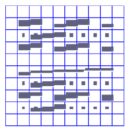
Figure 1. High contrast coefficient.

In the following we compute the norm of the error $e=u^{*}_{h}-u_{H}$ between the fine-scale solution obtained by solving (3) and the coarse-grid solution $u_{H}$, which is one of the following coarse-grid function: 1. $u_{H}^{ms,I}$ solution of (16), 2. $u_{H}^{ms,II}$ the solution of (19), or 3. $u_{H}^{ms,III}$ the solution of (23). The total error is $\|e\|_{h,1}^{2}$ where $\|\cdot\|_{h,\delta}^{2}$ defined in (11). The relative error is computed as $\|e\|_{h,1}^{2}/\|u^{*}_{h}\|_{h,1}^{2}$. The error is divided into two quantities:

• Interior Error: (square of the) broken $H^{1}-$semi-norm of the error

  $$\sum_{i=1}^{N}a_{i}(e,e)=\sum^{N}_{i=1}\parallel\kappa_{i}^{\frac{1}{2}}\nabla e_{i}\parallel^{2}_{L^{2}(\Omega_{i})}.$$

• Interface Error: (square of the) $L^{2}-$norm of the jump of the error across the edges

  $$\sum_{i=1}^{N}\sum_{E_{ij}\subset\partial\Omega_{i}}\!\!\!\frac{1}{l_{ij}}\frac{1}{h_{ij}}\int_{E_{ij}}\kappa_{ij}(e_{i}-e_{j})^{2}.$$

• Energy error: (square of the) DG bilinear form, that is, $a_{h}^{DG}(e,e)$.

4.1. Fine-grid snapshot space and original eigenvalue problem

In this Subsection we present the numerical experiments for the method introduced in Subsection 3.1 and show the error obtained when the dimension of the coarse space is increased.

First, we recall that for high-contrast problems we include the eigenvectors corresponding to small eigenvalues (that asymptotically vanish as the contrast increases). We denote by $L_{i}^{small}$ the number of these small eigenvalues in $\Omega_{i}$. To see the effect of adding more basis functions, we select additional $L_{i}^{add}$ eigenvalues so the total number of eigenvalues selected in the block $\Omega_{i}$ is $L^{small}_{i}+L^{add}_{i}$. We show that the error decays as $L_{i}^{add}$ increases. For the coefficient $\kappa(x)$ and coarse mesh shown on Figure 1 there is only one such and eigenvalue in each coarse-grid block $\Omega_{i}$ and therefore $L_{i}^{small}=1$, $i=1,2,\dots,N$. Figure 2 illustrates the effect of using increasing number of eigenvectors in the solution. We show the fine-scale solution and coarse-scale solutions computed with three different coarse spaces $L_{i}^{add}=0,2,11$.

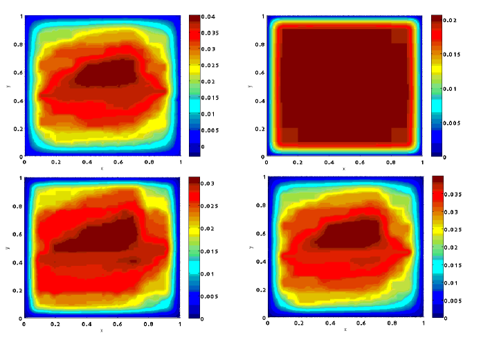
Figure 2. Illustration of fine and coarse solutions. Fine-scale solution $u^{*}_{h}$ (top left). Coarse-scale solution $u_{H}^{ms,I}$ with $L_{i}^{add}=0$ eigenvalues (top right). Coarse-scale solution $u_{H}^{ms,I}$ with $L_{i}^{add}=3$ eigenvalues (bottom left). Coarse-scale solution $u_{H}^{ms,I}$ with $L_{i}^{add}=11$ eigenvalues (bottom right).

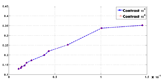
Figure 3. Total error of Method I (in Section 3.1) vs. $1/\lambda_{min}$. Here $h=1/100$ and the contrast is $10^{6}$. Coarse mesh size $H=1/10$ and contrast $10^{4}$ and $10^{6}$.

Table 1. Numerical results for the Method I (see Section 3.1). Here, $h=1/100$, $H=1/10$, $\mu=10^{4}$ and $\mu=10^{6}$ (in parenthesis)

$L_{i}^{add}$	Dim.	Interface error	Interior error	Total error	$\lambda_{\min}$
0	100 (100)	0.026 (0.026)	0.326 (0.326)	0.3522 (0.3522)	689.4 ( 689.3)
2	300 (300)	0.031 (0.032)	0.221 (0.220)	0.2523 (0.2516)	1562.2 (1561.7)
4	500 (500)	0.028 (0.029)	0.171 (0.170)	0.1991 (0.1984)	2607.5 (2607.0)
6	700 (700)	0.027 (0.027)	0.133 (0.131)	0.1600 (0.1581)	5199.4 (5199.3)
8	900 (900)	0.026 (0.027)	0.114 (0.113)	0.1399 (0.1392)	7237.9 (7237.6)
10	1100 (1100)	0.025 (0.025)	0.104 (0.103)	0.1293 (0.1283)	9509.1 (9509.0)

The results for the computation of interior and interface errors are presented in Table 1 for $h=1/100$ and $H=1/10$ and two different contrasts. The convergence with respect to the minimum left out eigenvalue is shown in Figure 3 (left). In this case, we solve a $100\times 100$ eigenvalue problem in each coarse block. From the results we see convergence to the reference solution (fine-grid solution). We also observe error decay proportional to the minimum left out eigenvalue across all coarse blocks. In particular, for $H=1/10$, we need only 3 or 4 additional functions to get an interior error or the order of $17\%$. This error is computed with respect to the fine-grid solution with fine-grid parameter $h=1/100$. Note that, in this case, we have total of four or five basis functions per subdomain which is comparable to the number of degrees of freedom of a classical DG method on the coarse grid.

4.2. Error vs. coarse problem penalty scaling

Now we test the error when we change the scaling of the penalty.

We recall that the fine-scale problem in (3) uses a penalty term scaled by $\delta\frac{1}{l_{ij}}\frac{1}{h_{ij}}$. In the classical SIPG formulation on the coarse grid one uses a penalty scaled by $\delta\frac{1}{l_{ij}}\frac{1}{H}.$ Here we experiment by computing the coarse solutions with several penalties in the range from $1/H$ to $1/h$ to identify a good penalty parameter for the coarse problem.

Figure 4. The error for values of $L_{i}^{add}=0,1,\dots,10$ and the two different penalty scalings: $\frac{\delta}{h}$ and $\frac{\delta}{H}.$ Here $h=1/100$, $H=1/10$ and $\eta=10^{4}$.

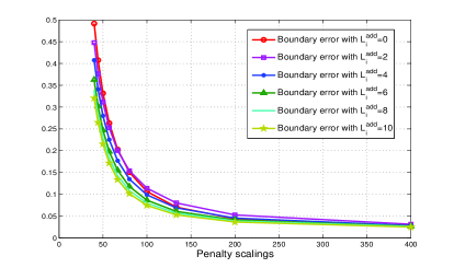
Figure 5. The error for Method I (in Section 3.1 vs penalty scaling for different values of $L_{i}^{add}$ . Here $h=1/100,$ $H=1/10$ and $\eta=10^{4}$. The interior error (left) and the boundary error (right).

For this experiment we set the contrast $\eta=10^{4}$, $M=10$, $n_{i}=10$, $i=1,\dots,N$ (and thus $H=1/10$ and $h=1/100$). Then, recalling that $\delta=4$ for the numerical experiments, we have $\delta\frac{1}{H}=40$ and $\delta\frac{1}{h_{ij}}=400$. For these two choices of the penalty in Figure 4 we show the decay of the interior and interface error when adding more eigenfunctions. We observe a reduction of the error as we use more and more additional coarse-grid basis functions. Also, we observe that the interior error are of comparable size (with either scaling) and that the interface error is bigger if we use the coarse penalty scaling.

We fix the number of additional eigenvectors $L_{i}^{add}$ and compute the interior and boundary errors when the coarse solution is computed with different penalties. We note that the fine-scale solution is computed with the fine-grid scaling of the penalty bilinear form. We repeat this experiments with $L_{i}^{add}=0,1,\dots,10$. Results are shown on Figure 5. From these results we observe that the boundary error for the coarse-grid solution is more sensitive to the variations in the scaling of the penalty. Indeed, for example $M=10$, with $L_{i}^{add}=4$, $i=1,\dots,N$, the optimal penalty coefficient is approximately $70$. These set of experiments demonstrates that one needs to properly choose the penalty parameter in order to balance boundary and interior errors.

4.3. Fine-grid snapshot space and amended eigenvalue problem

Here we consider the method introduced in Subsection 3.2. We repeat the experiment described in Subsection 4.1.

Table 2. Numerical results for Method II (Subsection 3.2) with increasing dimension of the coarse space, $h=1/100$, $H=1/10$, and $\eta=10^{4}$.

$L_{i}^{add}$	Dim	Interface	Interior	Total	Energy	$\lambda_{\min}$
0	100	0.0318	0.2854	0.3172	0.3172	0.0528
2	300	0.0342	0.1679	0.2020	0.2646	0.0933
4	500	0.0257	0.1066	0.1323	0.1793	0.1165
6	700	0.0214	0.0800	0.1014	0.1444	0.2459
8	900	0.0194	0.0581	0.0775	0.1164	0.3514
10	1100	0.0185	0.0566	0.0751	0.1132	0.4551

The results are displayed in Table 2 for contrast $\eta=10^{4}$. Similar results where observed for higher contrast. We observe error reduction when next eigenfunctions are added. Note that the results obtained by using the amended eigenvalue problem in Subsection 3.2 are slightly better. In this case our numerical results verify our theoretical error estimates in Theorem 3.5. Note that we report the energy error.

4.4. Local solutions as snapshot space

Next, we consider the snapshot space given as in Subsection 3.3 that consists of $a_{i}-$harmonic functions defined in (20). We note that this space of snapshots are used in the generalized multiscale finite element method for wave equation in [10]. The objective of presenting these results is to show that our proposed DG method is flexible and one can use various snapshot spaces.

Table 3. Numerical results for Method III (see Subsection 3.3) with increasing dimension of the coarse space, $h=1/100$, $H=1/10$ and $\eta=10^{4}$.

$L_{i}^{add}$	Dim	Interface	Interior	Total	Energy	$\lambda_{\min}$
0	100	0.032	0.285	0.317	0.373	0.0528
2	300	0.034	0.168	0.202	0.265	0.0933
4	500	0.026	0.107	0.133	0.181	0.1165
6	700	0.021	0.079	0.101	0.144	0.2459
8	900	0.019	0.058	0.077	0.116	0.3514
10	1100	0.018	0.057	0.075	0.114	0.4552

In Table 3, we present the numerical results with contrast $\eta=10^{4}$. Note, that we have obtained similar results for contrast $\eta=10^{6}$ (not reported here). In this example, we choose $H=1/10$ and the same setup as in the previous section. From these results we observe convergence to the fine-grid solution of (3). We also observe that the error is inversely proportional to the $\lambda_{min}$ (the minimum left out eigenvalue). Note that, we are reporting the error not with respect to the reference solution (on the snapshot space) but with respect to the fine-grid solution. Nevertheless, we observe good results.

We recall that we need to use the bilinear form $m^{\delta}_{i}$ in the eigenvalue problem in order to obtain error estimates. We also observe convergence in the numerical tests if we use $m_{i}$ bilinear form (instead of $m^{\delta}_{i}$) in the snapshot space of harmonic functions. These results are reported in Table 4.

Table 4. Numerical results for snapshot space and bilinear form $m_{i}$ (instead of $m^{\delta}_{i}$). Here $h=1/100$, $H=1/10$, and $\eta=10^{4}$.

$L_{i}^{add}$	Dim.	Interface	Interior	Total
2	300	0.0301	0.1750	0.2051
4	500	0.0278	0.1104	0.1382
6	700	0.0257	0.0905	0.1162
8	900	0.0243	0.0763	0.1007
10	1100	0.0223	0.0663	0.0986

5. Discussions on the convergence

In this section, we discuss the convergence of the proposed discontinuous multiscale finite element method. For the multiscale method in Section 3.2, we derived error estimates in Theorem 3.5. Similar result holds for the coarse space described in Section 3.3. Despite of the fact we do not write an error estimate for the multiscale space in Section 3.1, which uses simple weighted eigenvalue problems, we verified convergence in the numerical experiments. Moreover, we observe that the interface error due to penalty term is smaller than the interior error calculated with the energy norm (see Table 3). This indicates that once we have sufficient number of multiscale basis functions per coarse region (that are selected properly with our spectral problem) the interface error is dominated by the interior error. Consequently, one can argue that the local basis function construction should mostly take into account the approximation property within coarse regions the idea that we follow in this paper. The proposed eigenvalue problem attempts eliminating some interior degrees of freedom via an (interior and a boundary) mass matrix as discussed in our previous papers, e.g. [15, 20]. By selecting mass matrix carefully in the local spectral problem, we represent piecewise constant functions within high-conductivity inclusions as the exact solution becomes almost constant within these regions. Note that without the $\kappa$ (or $\kappa_{ij}$) weight in the mass bilinear form, we will be selecting large number of important modes (all fine-grid degrees of freedom within high-conductivity regions according to previous studies).

We have amended the local spectral problem with a mass term on the boundary (see Section 3.2 and 3.3) in order to obtain error estimates in terms of the local energy captured by the local space. A number of other similar eigenvalue problems that we tried, including adding some of the penalty terms in the eigenvalue problem, produced less satisfactory results.

As we observe from our numerical results that the penalty does not need to be very large. Even though the boundary error decreases, it is much lower than the interior error for relatively small penalty terms. Thus, if a small penalty term is preferred (e.g., for time-dependent problems), then one can attempt to find an optimal penalty. For the steady state problem considered in this paper, we do not investigate this problem. We believe that other appropriate techniques for coupling discontinuous spectral basis functions should be also considered. For instance, formulations that avoid the use of artificial penalty terms and use approaches such as hybridized discontinuous Galerkin methods, [11], or mortar methods, [6]. This is object of current research.

One can choose other multiscale spaces such that to achieve higher accuracy with lower degrees of freedom. For example, as we show that using proper eigenvalue problem one can improve the error. Error to a reference solution can also be improved by selecting appropriate snapshot spaces. In general, the choice of snapshot space depends on the input space as discussed in Introduction (see also [17] and the local solution space which this input space gives). Here, we do not explore the choice of snapshot spaces since our goal is to show that Discontinuous Galerkin provides a nice framework to couple discontinuous basis functions computed locally.

6. Acknowledgements

Y. Efendiev’s work is partially supported by the DOE and NSF (DMS 0934837 and DMS 0811180). J.Galvis would like to acknowledge partial support from DOE. R. Lazarov’s research was supported in parts by NSF (DMS-1016525).

This publication is based in part on work supported by Award No. KUS-C1-016-04, made by King Abdullah University of Science and Technology (KAUST).

We are grateful to Mr. Chak Shing Lee for implementing one of the methods and providing the results reported in Table 4.

References

- [1] J.E. Aarnes. On the use of a mixed multiscale finite element method for greater flexibility and increased speed or improved accuracy in reservoir simulation. SIAM J. Multiscale Modeling and Simulation, 2:421–439, 2004.
- [2] J.E. Aarnes and Y. Efendiev. Mixed multiscale finite element for stochastic porous media flows. SIAM J. Sci. Comput., 30 (5):2319–2339, 2008.
- [3] T. Arbogast. Analysis of a two-scale, locally conservative subgrid upscaling for elliptic problems. SIAM J. Numer. Anal., 42(2):576–598 (electronic), 2004.
- [4] T. Arbogast and K.J. Boyd. Subgrid upscaling and mixed multiscale finite elements. SIAM J. Numer. Anal., 44(3):1150–1171 (electronic), 2006.
- [5] T. Arbogast and M.S.M. Gomez. A discretization and multigrid solver for a Darcy-Stokes system of three dimensional vuggy porous media. Comput. Geosci., 13(2):331–343, 2009.
- [6] T. Arbogast, G. Pencheva, M.F. Wheeler, and I. Yotov. A multiscale mortar mixed finite element method. Multiscale Model. Simul., 6(1):319–346, 2007.
- [7] D.N. Arnold, F. Brezzi, B. Cockburn, and L.D. Marini. Unified analysis of discontinuous Galerkin methods for elliptic problems. SIAM J. Numer. Anal., 39(5):1749–1779, 2001/02.
- [8] S. Boyaval, C. LeBris, T. Lelièvre, Y. Maday, N. Nguyen, and A. Patera. Reduced basis techniques for stochastic problems. Archives of Computational Methods in Engineering, 17:435–454, 2010.
- [9] C.-C. Chu, I. G. Graham, and T.-Y. Hou. A new multiscale finite element method for high-contrast elliptic interface problems. Math. Comp., 79(272):1915–1955, 2010.
- [10] E.T. Chung, Y. Efendiev, and W.T. Leung. Generalized multiscale finite element method for wave propagation. (in progress).
- [11] B. Cockburn, J. Gopalakrishnan, and R.D. Lazarov. Unified hybridization of discontinuous Galerkin, mixed, and continuous Galerkin methods for second order elliptic problems. SIAM J. Numerical Analysis, 47(2):1319–1365, 2009.
- [12] M. Dryja. On discontinuous Galerkin methods for elliptic problems with discontinuous coefficients. Comput. Methods Appl. Math., 3(1):76–85 (electronic), 2003. Dedicated to Raytcho Lazarov.
- [13] W. E and B. Engquist. Heterogeneous multiscale methods. Comm. Math. Sci., 1(1):87–132, 2003.
- [14] J. Eberhard and G. Wittum. A coarsening multigrid method for flow in heterogeneous porous media. In Multiscale methods in science and engineering, volume 44 of Lect. Notes Comput. Sci. Eng., pages 111–132. Springer, Berlin, 2005.
- [15] Y. Efendiev and J. Galvis. Coarse-grid multiscale model reduction techniques for flows in heterogeneous media and applications. Chapter of Numerical Analysis of Multiscale Problems, Lecture Notes in Computational Science and Engineering, Vol. 83., pages 97–125.
- [16] Y. Efendiev and J. Galvis. A domain decomposition preconditioner for multiscale high-contrast problems. In Y. Huang, R. Kornhuber, O. Widlund, and J. Xu, editors, Domain Decomposition Methods in Science and Engineering XIX, volume 78 of Lect. Notes in Comput. Science and Eng., pages 189–196. Springer-Verlag, 2011.
- [17] Y. Efendiev, J. Galvis, and T. Hou. Generalized multiscale finite element methods. Submitted.
- [18] Y. Efendiev, J. Galvis, R. Lazarov, and J. Willems. Robust domain decomposition preconditioners for abstract symmetric positive definite bilinear forms. ESAIM Math. Model. Numer. Anal., 46(5):1175–1199, 2012.
- [19] Y. Efendiev, J. Galvis, and F. Thomines. A systematic coarse-scale model reduction technique for parameter-dependent flows in highly heterogeneous media and its applications. Accepted.
- [20] Y. Efendiev, J. Galvis, and X.H. Wu. Multiscale finite element methods for high-contrast problems using local spectral basis functions. Journal of Computational Physics, 230:937–955, 2011.
- [21] Y. Efendiev and T. Hou. Multiscale Finite Element Methods: Theory and Applications, volume 4 of Surveys and Tutorials in the Applied Mathematical Sciences. Springer, New York, 2009.
- [22] Y. Efendiev, T. Hou, and V. Ginting. Multiscale finite element methods for nonlinear problems and their applications. Comm. Math. Sci., 2:553–589, 2004.
- [23] J. Galvis and Y. Efendiev. Domain decomposition preconditioners for multiscale flows in high contrast media. SIAM J. Multiscale Modeling and Simulation, 8:1461–1483, 2010.
- [24] I.G. Graham, P. O. Lechner, and R. Scheichl. Domain decomposition for multiscale PDEs. Numerische Mathematik, 106(4):589–626, 2007.
- [25] T. Hou and X.H. Wu. A multiscale finite element method for elliptic problems in composite materials and porous media. J. Comput. Phys., 134:169–189, 1997.
- [26] T. Hughes, G. Feijoo, L. Mazzei, and J. Quincy. The variational multiscale method - a paradigm for computational mechanics. Comput. Methods Appl. Mech. Engrg., 166:3–24, 1998.
- [27] O. Iliev, R. Lazarov, and J. Willems. Variational multiscale finite element method for flows in highly porous media. Multiscale Model. Simul., 9(4):1350–1372, 2011.
- [28] P. Jenny, S.H. Lee, and H. Tchelepi. Multi-scale finite volume method for elliptic problems in subsurface flow simulation. J. Comput. Phys., 187:47–67, 2003.
- [29] Y. Maday. Reduced-basis method for the rapid and reliable solution of partial differential equations. Downloadable at http://hal.archives-ouvertes.fr/hal-00112152/, 7 2006.
- [30] A. Toselli and O. Widlund. Domain decomposition methods – Algorithms and Theory, volume 34 of Computational Mathematics. Springer-Verlag, 2005.
- [31] P.S. Vassilevski. Multilevel block-factrorization preconditioners. Matrix-based analysis and algorithms for solving finite element equations. Springer-Verlag, New York, 2008.
- [32] P.S. Vassilevski. Coarse spaces by algebraic multigrid: multigrid convergence and upscaling error estimates. Adv. Adapt. Data Anal., 3(1-2):229–249, 2011.
- [33] M.F. Wheeler, G. Xue, and I. Yotov. A multiscale mortar multipoint flux mixed finite element method. ESAIM Math. Model. Numer. Anal., 46(4):759–796, 2012.