Nonuniqueness of the $\mathcal{C}$ operator in $\mathcal{P}\mathcal{T}$-symmetric quantum mechanics

Abstract

The $\mathcal{C}$ operator in $\mathcal{PT}$-symmetric quantum mechanics satisfies a system of three simultaneous algebraic operator equations, $\mathcal{C}^{2}=1$, $[\mathcal{C},\mathcal{PT}]=0$, and $[\mathcal{C},H]=0$. These equations are difficult to solve exactly, so perturbative methods have been used in the past to calculate $\mathcal{C}$. The usual approach has been to express the Hamiltonian as $H=H_{0}+\epsilon H_{1}$, and to seek a solution for $\mathcal{C}$ in the form $\mathcal{C}=e^{Q}\mathcal{P}$, where $Q=Q(q,p)$ is odd in the momentum $p$, even in the coordinate $q$, and has a perturbation expansion of the form $Q=\epsilon Q_{1}+\epsilon^{3}Q_{3}+\epsilon^{5}Q_{5}+\ldots$. [In previous work it has always been assumed that the coefficients of even powers of $\epsilon$ in this expansion would be absent because their presence would violate the condition that $Q(p,q)$ is odd in $p$.] In an earlier paper it was argued that the $\mathcal{C}$ operator is not unique because the perturbation coefficient $Q_{1}$ is nonunique. Here, the nonuniqueness of $\mathcal{C}$ is demonstrated at a more fundamental level: It is shown that the perturbation expansion for $Q$ actually has the more general form $Q=Q_{0}+\epsilon Q_{1}+\epsilon^{2}Q_{2}+\ldots$ in which all powers and not just odd powers of $\epsilon$ appear. For the case in which $H_{0}$ is the harmonic-oscillator Hamiltonian, $Q_{0}$ is calculated exactly and in closed form and it is shown explicitly to be nonunique. The results are verified by using powerful summation procedures based on analytic continuation. It is also shown how to calculate the higher coefficients in the perturbation series for $Q$.

I Introduction

The properties of $\mathcal{PT}$-symmetric Hamiltonians have been observed in a wide variety of laboratory experiments R1 ; R2 ; R3 ; R4 ; R5 ; R6 ; R7 ; R8 ; R9 ; R10 . For a $\mathcal{PT}$-symmetric Hamiltonian having an unbroken $\mathcal{PT}$ symmetry a linear $\mathcal{PT}$-symmetric operator $\mathcal{C}$ exists that obeys the following three algebraic equations:

$$\mathcal{C}^{2} = 1,$$ (1)

$$\left[\mathcal{C},\mathcal{PT}\right] = 0,$$ (2)

$$\left[\mathcal{C},H\right] = 0.$$ (3)

Constructing the $\mathcal{C}$ operator is the key step in showing that time evolution for a non-Hermitian $\mathcal{PT}$-symmetric Hamiltonian is unitary R11 ; R12 .

The $\mathcal{C}$ operator for a few nontrivial quantum-mechanical models has been calculated exactly R13 ; R14 ; R15 ; R16 ; R17 by solving (1)-(3). However, in general this system of equations is extremely difficult to solve analytically. Therefore, in most cases a perturbative approach has been adopted for the solution of these equations R18 ; R19 ; R20 ; R21 ; R22 .

The standard approach to solving (1)-(3) has been to express the $\mathcal{C}$ operator in a simple and natural form as an exponential of a Dirac Hermitian operator $Q$ multiplying the parity operator $\mathcal{P}$:

$$\mathcal{C}=e^{Q}\mathcal{P}.$$ (4)

Note that $e^{Q/2}$ is precisely the metric operator $\eta$ discussed in Refs. R23 ; R24 ; R25 ; R26 ; R27 ; R28 . This operator can be used to construct a similarity transformation that maps the non-Hermitian Hamiltonian $H$ to an isospectral Hermitian Hamiltonian R29 . If we seek a solution for $\mathcal{C}$ in the form (4), we find that (1) and (2), which can be thought of as kinematical equations because they hold for all choices of $H$, imply that $Q(p,q)$ is an odd function of the momentum operator $p$ and an even function of the coordinate operator $q$ R11 ; R12 . The problem is then reduced to finding the solution to (3), which can be thought of as a dynamical equation because it refers to the Hamiltonian $H$.

It is difficult to find a closed-form analytical solution to (3). However, in the past this equation has been solved perturbatively as follows: Express the Hamiltonian in the form $H=H_{0}+\epsilon H_{1}$ and treat $\epsilon$ as a small parameter. Then, seek $Q$ as a formal perturbation series in odd powers of $\epsilon$:

$$Q(p,q)=\sum_{j=0}^{\infty}\epsilon^{2j+1}Q_{2j+1}(p,q).$$ (5)

The obvious question to ask is, Why do only odd powers in $\epsilon$ appear in the perturbation series (5)? The explanation that has been given in the past is that even powers of $\epsilon$ are excluded from the series because $Q(p,q)$ is required to be odd in $p$ and even in $q$. The reasoning goes as follows: In the quantum-mechanical cases that have been studied so far, such as $H=H_{0}+i\epsilon q$ and $H=H_{0}+i\epsilon q^{3}$, the unperturbed Hamiltonian $H_{0}=\mbox{$\textstyle{\frac{1}{2}}$}p^{2}+\mbox{$\textstyle{\frac{1}{2}}$}q^{2}$ is the harmonic-oscillator Hamiltonian. If there were a term $Q_{0}\epsilon^{0}$ in the series (5), then $Q_{0}$ would satisfy the commutation relation $[Q_{0},H_{0}]=0$. The vanishing of this commutator implies that $Q_{0}$ is a function of $H_{0}$, and thus it is an even function of $p$, which shows that $Q_{0}=0$. Once it is established that $Q_{0}=0$, it is relatively easy to show (see Ref. R15 , for example) that $Q_{2j}=0$ ($j=1,\,2,\,3,\,\ldots$). We show in this paper that this argument is actually incorrect; there are indeed solutions to the commutator equation $[Q_{0},H_{0}]=0$ that are odd in $p$ – infinitely many such solutions, in fact. It is precisely because of the existence of these odd-$p$ solutions that the $\mathcal{C}$ operator is nonunique.

It has recently become clear that the nonuniqueness of the $\mathcal{C}$ operator has important implications for the mathematical and physical interpretation of $\mathcal{PT}$-symmetric quantum mechanics R30 ; R31 ; R32 . In Ref. R31 it is shown that if the $\mathcal{C}$ operator is nonunique, then it is unbounded, and in this paper we verify this result explicitly.

The paper R33 is relevant because it discusses for the first time the existence of multiple (nonunique) solutions to the commutator equation (3). In Ref. R33 it is shown that the inhomogeneous commutator equation $[Q_{1},H_{0}]=2H_{1}$ has an infinite number of particular solutions, which differ from one another by solutions to the associated homogeneous commutator equation $[X,H_{0}]=0$, and it recognizes that the solutions $X$ are not necessarily functions of $H_{0}$ only. The importance of nonunique solutions to commutator equations is also central to Ref. R34 , where a particular time-operator solution $\Theta$ to the inhomogeneous commutator equation $[\Theta,H]=i$ is called minimal and a classification of the infinite number of associated nonminimal solutions is given.

The approach used in the current paper is based on the recognition that finding multiple solutions for $Q_{1}$ in (5) is not the only way to demonstrate nonuniqueness. Here, we introduce a clearer and more fundamental way to explain the nonuniqueness of the $\mathcal{C}$ operator. We show that a more general way to represent $Q$ is by the expansion

$$Q(p,q)=\sum_{j=0}^{\infty}\epsilon^{j}Q_{j}(p,q)$$ (6)

in which all nonnegative integer powers of $\epsilon$ appear. An advantage of this new representation is that in the limit $\epsilon\to 0$ we obtain an infinite class of exact $\mathcal{C}$ operators for the quantum harmonic-oscillator Hamiltonian $H_{0}=\mbox{$\textstyle{\frac{1}{2}}$}p^{2}+\mbox{$\textstyle{\frac{1}{2}}$}q^{2}$. Then, once we have $Q_{0}$ for the harmonic-oscillator case, we can straightforwardly generalize this result and verify that the operator $\mathcal{C}$ is nonunique.

This paper is organized as follows: In Sec. II we show how to construct exact and explicit closed-form solutions that are odd in $p$ and even in $q$ to the homogeneous commutator equation $[Q_{0}(p,q),H_{0}]=0$. Our result is that there is a unique bounded $\mathcal{C}$ operator and a nonunique infinite class of unbounded $\mathcal{C}$ operators for the quantum harmonic oscillator. The techniques used in Sec. II involve the formal summation of infinite series of singular operators. However, in Sec. III we verify the validity of the formal calculations done in Sec. II by applying powerful summation techniques that are used to regulate divergent Feynman integrals. This verification leads us to conjecture that it may be possible to apply the principles of summation theory to extend and generalize the rigorous notions of Cauchy sequences and completeness expansions, which are used in mathematical Hilbert-space theory, to divergent sequences and series of vectors. Next, in Sec. IV we develop the formal machinery needed to determine the higher coefficients $Q_{1}$, $Q_{2}$, $\ldots$, in the expansion (6), and in Sec. V we concentrate on calculating $Q_{1}(p,q)$ for the specific case $H_{1}=iq$. Finally, in Sec. VI we make some brief concluding remarks.

II Solutions to $[Q_{0}(p,q),H_{0}]=0$ that are odd in $p$ and even in $q$

A powerful strategy for solving operator equations of the form

$$[Q_{0}(p,q),H_{0}]=0$$ (7)

is to represent the solution $Q_{0}(p,q)$ as an infinite series of totally symmetric operator basis functions $T_{m,n}$. The operators $T_{m,n}$ are described in detail in Refs. R34 ; R35 ; R36 ; R37 . However, to make the presentation in this paper self-contained, we recall that for $m,n\geq 0$ the operator $T_{m,n}$ is defined as a symmetric average over all orderings of $m$ factors of $p$ and $n$ factors of $q$:

$$T_{1,1} = \mbox{$\textstyle{\frac{1}{2}}$}(pq+qp),$$

$$T_{1,2} = \textstyle{\frac{1}{3}}(pqq+qpq+qqp),$$

and so on. The operators $T_{m,n}$ obey simple commutation and anticommutation relations:

$$\left[p,T_{m,n}\right] = -inT_{m,n-1},$$

$$\left[q,T_{m,n}\right] = imT_{m-1,n},$$

$$\left\{p,T_{m,n}\right\} = 2T_{m+1,n},$$

$$\left\{q,T_{m,n}\right\} = 2T_{m,n+1},$$

$$\left[p^{2},T_{m,n}\right] = -2inT_{m+1,n-1},$$

$$\left[q^{2},T_{m,n}\right] = 2imT_{m-1,n+1},$$ (8)

where the curly brackets indicate anticommutators. The operator $T_{m,n}$ can be re-expressed in Weyl-ordered form R36 :

$$T_{m,n}=\frac{1}{2^{m}}\sum_{k=0}^{m}\binom{m}{k}p^{k}q^{n}p^{m-k}=\frac{1}{2^{n}}\sum_{k=0}^{n}\binom{n}{k}q^{k}p^{m}q^{n-k},$$ (9)

where $m,\,n=0,\,1,\,2,\,3,\,\cdots$. Introducing the Weyl-ordered form of $T_{m,n}$ allows one to extend the operators $T_{m,n}$ either to negative values of $n$ by using the first sum or to negative values of $m$ by using the second sum. The commutation and anticommutation relations in (8) remain valid when $m$ is negative or when $n$ is negative.

To find solutions that are odd in $p$ and even in $q$ to the commutator equation (7), we take $Q_{0}(p,q)$ to have the general form

$$Q_{0}^{(\gamma)}(p,q)=\sum_{k}a_{k}^{(\gamma)}T_{2\gamma+1-2k,2k},$$ (10)

where $\gamma=0,\,\pm 1,\,\pm 2,\,\ldots$ is a parameter. Substituting (10) into (7), we obtain the following two-term recursion relation for the coefficients $a_{k}^{(\gamma)}$:

$$a_{k+1}^{(\gamma)}(k+1)-(\gamma-k+1/2)a_{k}^{(\gamma)}=0\quad(k=0,1,2,\ldots).$$ (11)

This recursion relation is self-terminating; that is, if we choose $a_{-1}^{(\gamma)}=0$, then $a_{0}^{(\gamma)}$ is an arbitrary constant, $a_{k}^{(\gamma)}$ vanishes for $k<0$, and $a_{k}^{(\gamma)}$ for $k>0$ is determined in terms of $a_{0}^{(\gamma)}$ as the solution to the recursion relation (11):

$$a_{k}^{(\gamma)}=a_{0}^{(\gamma)}(-1)^{k}\frac{\Gamma(k-\gamma-1/2)}{k!\Gamma(-\gamma-1/2)}\quad(k=0,1,2,\ldots).$$ (12)

The series (10) with coefficients (12) can be summed as a binomial expansion:

$$\sum_{k=0}^{\infty}a_{k}^{(\gamma)}x^{2k}=a_{0}^{(\gamma)}\left(1+x^{2}\right)^{\gamma+1/2}.$$ (13)

Thus, for each $\gamma\geq 0$ the odd-$p$ and even-$q$ one-parameter family of solutions to the homogeneous commutator equation (7) is

$$Q_{0}^{(\gamma)}=\frac{a_{0}^{(\gamma)}}{2^{2\gamma+2}}\left\{\ldots\left\{\left\{\left(1+q\frac{1}{p}q\frac{1}{p}\right)^{\gamma+1/2}+\left(1+\frac{1}{p}q\frac{1}{p}q\right)^{\gamma+1/2},p\right\},p\right\}\dots,p\right\}_{(2\gamma+1)~{}{\rm times}},$$ (14)

where we have used the identity R34

$$T_{-n,n}=\frac{1}{2}\left(q\frac{1}{p}\right)^{n}+\frac{1}{2}\left(\frac{1}{q}p\right)^{n}.$$ (15)

As stated in Sec. I, we can see that while $Q_{0}^{(\gamma)}$ commutes with the Hamiltonian $H_{0}=\mbox{$\textstyle{\frac{1}{2}}$}p^{2}+\mbox{$\textstyle{\frac{1}{2}}$}q^{2}$, it is not a function of $H_{0}$ because by construction it is odd in $p$. Furthermore, while the construction of the solutions in (14) involves series in inverse powers of $p$, these solutions are well behaved as $p\to 0$. To see explicitly the oddness in $p$ we display the solution corresponding to $\gamma=0$:

$$Q_{0}^{(0)}=\frac{1}{4}a_{0}^{(0)}\left(\sqrt{1+q\frac{1}{p}q\frac{1}{p}}\,\,p+p\,\sqrt{1+q\frac{1}{p}q\frac{1}{p}}+\sqrt{1+\frac{1}{p}q\frac{1}{p}q}\,\,p+p\,\sqrt{1+\frac{1}{p}q\frac{1}{p}q}\right).$$ (16)

In the classical limit for which $p$ and $q$ become commuting numbers, this solution becomes

$$Q_{0,{\rm classical}}^{(0)}=a_{0}^{(0)}{\rm sgn}(p)\sqrt{p^{2}+q^{2}};$$ (17)

the oddness in $p$ is evident.

It is important to point out that for the harmonic oscillator, which corresponds to $\epsilon=0$, the metric operator $\eta=e^{Q_{0}}$ is just unity when $Q_{0}=0$. Thus, the metric operator is bounded of this special case. However, for $Q_{0}$ in (16), the metric operator is no longer bounded, but rather for large $q$ it behaves like $e^{q}$ and for large $p$ it behaves like $e^{p}$. Needless to say, since there is an infinite number of possible choices for $Q_{0}$, there is an infinite number of possible metric operators. Only one of the metric operators is bounded R38 ; R39 ; R40 .

III Using summation techniques to verify results of Sec. II

We observed in Sec. II that even though solutions $Q_{0}^{(\gamma)}$ in (14) were constructed by performing a formal infinite sum over arbitrary powers of the inverse momentum operator $1/p$, these solutions are well behaved as $p\to 0$. However, the calculations in Sec. II are certainly not rigorous. The aim of this section is to provide mathematical support for the validity of the formulas in (14). Specifically, since the $\mathcal{C}$ operator commutes with the Hamiltonian, the $n$th eigenstate $|\psi_{n}\rangle$ of the Hamiltonian must also be an eigenstate of $\mathcal{C}$. We expect that the eigenvalue of $|\psi_{n}\rangle$ is $(-1)^{n}$. For this to be true, $|\psi_{n}\rangle$ must be an eigenstate of $Q_{0}^{(\gamma)}$ with eigenvalue $0$ for all $n$:

$$Q_{0}^{(\gamma)}|\psi_{n}\rangle=0.$$ (18)

In this section we show by explicit calculation in which we use powerful summation techniques that this is indeed the case. Here, we limit our calculation to the case $\gamma=0$. We first consider the ground state $|\psi_{0}\rangle$ and then generalize to the $n$th eigenstate.

From (10) and (12) we see that $Q_{0}^{(0)}$ is given by

$$Q_{0}^{(0)}=\sum_{k=0}^{\infty}a_{k}T_{1-2k,2k},\qquad a_{k}=a_{0}\frac{(-1)^{k}\Gamma(k-1/2)}{2\sqrt{\pi}k!}.$$ (19)

Also, the unnormalized eigenfunctions of the harmonic-oscillator Hamiltonian in coordinate space are given by $\psi_{n}(q)=H_{n}(q)e^{-q^{2}/2}$. While the formal sum in (19) can be written as (16), it is difficult to use this result to verify the eigenvalue equation (18). A better strategy is to calculate the action of each term in the sum in (19) on the eigenstates and then to perform the summation over $k$.

Because inverse powers of the momentum operator arise in (19), it is most convenient to work in the momentum representation, where the eigenvalue equation (18) becomes

$$\langle p|Q_{0}^{(0)}|\psi_{n}\rangle=\frac{1}{4}\sum_{k=0}^{\infty}a_{k}(-1)^{k}\left\{p\left(\frac{1}{p}\partial_{p}\right)^{2k}+p\left(\partial_{p}\frac{1}{p}\right)^{2k}+\left(\frac{1}{p}\partial_{p}\right)^{2k}p+\left(\partial_{p}\frac{1}{p}\right)^{2k}p\right\}\tilde{\psi}_{n}(p)=0,$$ (20)

where we have used (15) and the third formula in (8). Here, $\tilde{\psi}_{n}(p)=(-i)^{n}\psi_{n}(p)$, where $\tilde{\psi}$ is the Fourier transform of $\psi$.

III.1 Ground state $\psi_{0}$

Let we first study the simplest case $n=0$. We can see that the action of each term in the series expansion (20) on the eigenstate $\psi_{0}$ produces more and more negative powers of the momentum $p$:

$$Q_{0}^{(0)}(p)\tilde{\psi}_{0}(p) = \frac{1}{4}\left\{4p\,a_{0}-\left(4p+\frac{2}{p^{3}}\right)a_{1}+\left(4p+\frac{12}{p^{3}}+\frac{48}{p^{5}}+\frac{90}{p^{7}}\right)a_{2}-\left(4p+\frac{30}{p^{3}}+\frac{240}{p^{5}}+\frac{1350}{p^{7}}+\frac{5040}{p^{9}}\right)a_{3}\right.$$

$$+ \left.\left(4p+\frac{56}{p^{3}}+\frac{672}{p^{5}}+\frac{6300}{p^{7}}+\frac{47040}{p^{9}}+\frac{264600}{p^{11}}+\frac{997920}{p^{13}}+\frac{1891890}{p^{15}}\right)a_{4}-\ldots\right\}e^{-p^{2}/2}.$$

We can rearrange the series in (LABEL:e21) to read

$$Q_{0}^{(0)}(p)\tilde{\psi}_{0}(p)=\frac{1}{4}\left\{4p\sum_{k=0}^{\infty}(-1)^{k}a_{k}-\sum_{k=0}^{\infty}\frac{(-1)^{k}}{p^{4k+3}}a_{k+1}P_{2k}(2p^{2})\right\}e^{-p^{2}/2},$$ (22)

where $P_{n}(y)$ are polynomials:

$$P_{n}(y)=\sum_{\alpha=0}^{n}\frac{(n+1)!(2\alpha+2)!}{2^{\alpha}\alpha!(\alpha+2)!(n-\alpha)!}y^{n-\alpha}.$$ (23)

To verify that $Q_{0}^{(0)}(p)\tilde{\psi}_{0}(p)=0$, we must show that

$$4\pi p\sum_{k=0}^{\infty}\frac{\Gamma(k-1/2)}{k!}-\frac{1}{p^{3}}\sum_{\alpha=0}^{\infty}\frac{1}{p^{2\alpha}}\frac{(2\alpha+2)!}{\alpha!(\alpha+2)!2^{\alpha}}\sum_{k=0}^{\infty}\frac{\Gamma(2k+1)\Gamma(k+3/2)}{\Gamma(k+1)\Gamma(2k-\alpha+1)}=0,$$ (24)

where we have substituted the above formulas for the polynomials $P_{n}$ and the coefficients $a_{k}$. It is easy to verify that the exact sum of the convergent series $\sum_{k=0}^{\infty}\Gamma(k-1/2)/k!$ is zero. However, the series $\sum_{k=0}^{\infty}\frac{\Gamma(2k+1)\Gamma(k+3/2)}{\Gamma(k+1)\Gamma(2k-\alpha+1)}$ is divergent for $\alpha\geq 3/2$. Therefore, we must introduce a summation procedure to make sense of this series.

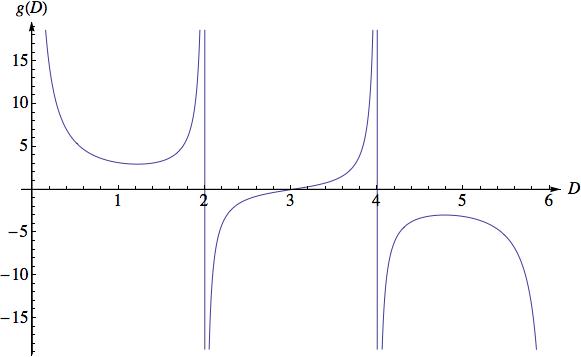
Figure 1: A plot of $g(D)$ in (26) for $0<D<6$. Note that $g(3)$ vanishes even though the integrand of $I(D)$ in (25) is strictly positive for all $D$. This shows that the notions of positivity and negativity evaporate in the case of a divergent integral representation.

Our summation procedure is a discrete variant of dimensional continuation, a technique that is used to interpret divergent Feynman integrals. To illustrate our approach, let us consider the following $D$-dimensional integral:

$$I(D)=\int d^{D}x\frac{x^{2}+3}{(x^{2}+1)^{2}}.$$ (25)

This integral converges for $D<2$ and its exact value is $I(D)=S_{D}\,g(D)$, where $S_{D}=2\pi^{D/2}/\Gamma(D/2)$ is the surface area of a $D$-dimensional sphere of radius $1$ and

$$g(D)=\frac{(3-D)\pi}{2\sin(\pi D/2)}.$$ (26)

Evidently, even though the integral representation for $I(D)$ diverges for $D\geq 2$, the function $I(D)$ is well defined and analytic in $D$ except for isolated simple poles. [Figure 1 gives a plot of $g(D)$ for $0<D<6$.] Observe that $I(D)$ vanishes for $D=3$. This result is surprising and somewhat counterintuitive because the integrand of $I(D)$ is strictly positive when $D=3$. The vanishing of $I(3)$ shows that when an integral representation is divergent we cannot draw qualitative conclusions regarding the sign of its value. (Indeed, the Borel sum of the series $1+2+4+8+\dots$ is uniquely $-1$ even though all of the terms in this divergent series are positive!)

We will now show that while the sum over $k$ in (24) diverges for $\alpha>-3/2$, we can evaluate the sum for $\alpha<-3/2$ and then use analytic continuation in $\alpha$ to sum the series for $\alpha=0,\,1,\,2,\,3,\,\ldots$. The surprising and counterintuitive result is that while the summand is positive for $2k+1>\alpha$, the sum of the (divergent) series vanishes for all nonnegative integer values of $\alpha$.

The divergent series to be summed is

$$F_{\alpha}=\sum_{k=0}^{\infty}\frac{\Gamma(2k+1)\Gamma(k+3/2)}{\Gamma(k+1)\Gamma(2k-\alpha+1)}.$$ (27)

To perform the sum we first express the coefficients in terms of the beta function:

$$B(x,y)=\frac{\Gamma(x)\Gamma(y)}{\Gamma(x+y)},$$ (28)

whose integral representation is

$$B(x,y)=\int_{0}^{1}dt\,t^{(x-1)}\,(1-t)^{(y-1)}\qquad({\rm Re}(x),~{}{\rm Re}(y)>0).$$ (29)

By multiplying and dividing $F_{\alpha}$ by $\Gamma(-\alpha)$ we obtain the result

$$F_{\alpha}=\frac{1}{\Gamma(-\alpha)}\sum_{k=0}^{\infty}\frac{\Gamma(k+3/2)}{\Gamma(k+1)}B(2k+1,-\alpha)=\frac{1}{\Gamma(-\alpha)}\sum_{k=0}^{\infty}\frac{\Gamma(k+3/2)}{\Gamma(k+1)}\int_{0}^{t}dt\,t^{2k}(1-t)^{-\alpha-1}.$$ (30)

We then use the binomial expansion

$$\sum_{k=0}^{\infty}\frac{\Gamma(k+3/2)}{k!}t^{2k}=\frac{\sqrt{\pi}}{2}(1-t^{2})^{-3/2}$$ (31)

to show that

$$F_{\alpha}=\frac{\sqrt{\pi}}{2\Gamma(-\alpha)}\int_{0}^{1}dt(1-t)^{-\alpha-5/2}(1+t)^{-3/2}=\frac{\sqrt{\pi}\,\Gamma(-\alpha-3/2)}{2\Gamma(-\alpha)}{}_{2}F_{1}\left(\frac{3}{2},1;-\alpha-\frac{1}{2},-1\right).$$ (32)

This function vanishes for all nonnegative integer values of $\alpha$ because the hypergeometric function is finite for these values of $\alpha$. In Fig. 2 we plot $F_{\alpha}$ for $-5\leq\alpha\leq 10$. Observe that $F_{\alpha}$ vanishes for $\alpha=0,\,1,\,2,\,\ldots$. Note also that $F_{\alpha}$ is singular at $\alpha=-3/2$, the value of $\alpha$ for which the series (27) begins to diverge. Interestingly, this function has double poles at the half-odd integers $\alpha=1/2,\,3/2,\,5/2,\,\ldots$. As $\alpha$ increases, the double poles begin to resemble single poles

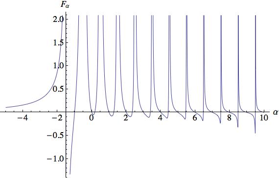
Figure 2: A plot of $F_{\alpha}$ in (32) for $-5<\alpha<10$. Note that $F_{\alpha}$ vanishes at every nonnegative integer. This happens because $\Gamma(-\alpha)$ in the denominator is infinite when $\alpha=0,\,1,\,2,\,\ldots$ and the hypergeometric function is finite. These zeros are all simple zeros, but the poles at the half-odd integers beginning with $1/2$ are all double poles, as is verified in Fig. 3.

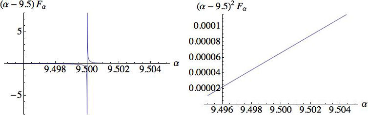
Figure 3: A blow-up of the region near $\alpha=9.5$ in Fig. 2. In the left panel is a plot of $(\alpha-9.5)F_{\alpha}$ for $9.496<\alpha<9.505$ and in the right panel is a plot of $(\alpha-9.5)^{2}F_{\alpha}$ for the same range of $\alpha$. Note that the left plot has a typical simple-pole behavior at $\alpha=9.5$ while the graph in the right panel is finite at $\alpha=9.5$.

III.2 Generalization: eigenvalue equation for $\psi_{n}$

In this subsection we study the action of the operator $Q^{(0)}_{0}$ on the $n$th eigenstates of the harmonic-oscillator Hamiltonian. We describe first the case for which $n$ is even. (The odd-$n$ case is treated in an identical fashion and is considered briefly at the end of this subsection.) For even $n$

$$Q_{0}^{(0)}\tilde{\psi}_{2n}=\left[-\sum_{k=1}^{\infty}\frac{(-1)^{k}}{p^{4k-1}}a_{k}J^{(n)}_{2k-1}(p^{2})+\sum_{j=0}^{n}p^{2j+1}\sum_{k=0}^{\infty}(-1)^{k}a_{k}S^{(n)}_{n-j}(k)\right]e^{-p^{2}/2}\quad(n=1,2,3,\ldots).$$ (33)

Both the sums over $k$ in (33) diverge for $\alpha=0,1,2,\ldots$ except for $j=n$ in the first series. (The special case $j=n$ gives the convergent series that was already considered in Subsec. III.1.) The divergent series can be evaluated by using the summation procedure that was introduced in the previous subsection. Following the procedure for the $n=0$ case, we will show that if we write (33) as

$$Q_{0}^{(0)}\tilde{\psi}_{2n}=\left[-\mathcal{N}^{(n)}+\sum_{j=0}^{n}p^{2j+1}\mathcal{M}^{(n,j)}\right]e^{-p^{2}/2},$$ (34)

then both $\mathcal{M}^{(n,j)}$ and $\mathcal{N}^{(n)}$ vanish for $n=1,2,\ldots$, $j=0,1,\ldots n$.

We first consider the series

$$\mathcal{N}^{(n)}=\sum_{k=1}^{\infty}\frac{(-1)^{k}}{p^{4k-1}}a_{k}J^{(n)}_{2k-1}(p^{2}),$$ (35)

where $J^{(n)}_{k}(x)$ are $k$th order polynomials that can be written as

$$J^{(n)}_{k}(x)=(2n-1)!!\frac{2^{n+1}}{\sqrt{\pi}}\sum_{\alpha=0}^{k}\frac{2^{\alpha}(k+1)!\Gamma(\alpha+1/2)}{(k-\alpha)!(n+\alpha+1)!}E_{n,\alpha}(k)x^{k-\alpha},$$ (36)

and $E_{n,\alpha}(k)$ are polynomials of degree $n$ in the variable $k$. The first four polynomials are

$$E_{1,\alpha}(k) = 2(1-\alpha)k+\alpha^{2}-4\alpha,$$

$$E_{2,\alpha}(k) = (4\alpha-8)k^{2}-(4\alpha^{2}-20\alpha+4)k+\alpha^{3}-7\alpha^{2}+10\alpha,$$

$$E_{3,\alpha}(k) = (24-8\alpha)k^{3}+(12\alpha^{2}-72\alpha+24)k^{2}-(6\alpha^{2}-48\alpha^{2}+70\alpha-24)k+\alpha^{4}-9\alpha^{3}+20\alpha^{2}-48\alpha,$$

$$E_{4,\alpha}(k) = (16\alpha-64)k^{4}-(32\alpha^{2}-224\alpha+96)k^{3}+(24\alpha^{3}-216\alpha^{2}+320\alpha-224)k^{2}$$ (37)

$$-(8\alpha^{4}-80\alpha^{3}+176\alpha^{2}-536\alpha+96)k+\alpha^{5}-10\alpha^{4}+23\alpha^{3}-158\alpha^{2}+216\alpha.$$

In terms of $E_{n,\alpha}(2k-1)=\sum_{\gamma=1}^{n}e_{\alpha,\gamma}k^{\gamma}$, the first term in (34) can be written as

$$\mathcal{N}^{(n)}=\frac{2}{\pi}(2n-1)!!\sum_{\alpha=0}^{\infty}\frac{2^{\alpha}}{p^{2\alpha+1}}\frac{\Gamma(\alpha+1/2)}{(n+\alpha+1)!}\sum_{\gamma=1}^{n}e_{\alpha,\gamma}\,\mathcal{N}_{\alpha,\gamma},$$ (38)

where $\mathcal{N}_{\alpha,\gamma}$ is given by

$$\mathcal{N}_{\alpha,\gamma}=\sum_{k=1}^{\infty}\frac{\Gamma\left(k-\frac{1}{2}\right)\Gamma(2k+1)}{\Gamma(k-1)\Gamma(2k-\alpha)}k^{\gamma}.$$ (39)

This is the divergent series that we need to study.

Because $\mathcal{N}_{\alpha,\gamma}$ is divergent for $\alpha\geq-5/2-\gamma$, we evaluate the sum for $\alpha<-5/2-\gamma$ and use analytic continuation in $\alpha$ to sum the series for $\alpha=0,1,2,\ldots$. Multiplying and dividing $\mathcal{N}_{\alpha,\gamma}$ by $\Gamma(-\alpha-1)$ and using the integral representation of the beta function $B$, we obtain

$$\mathcal{N}_{\alpha,\gamma}=\frac{1}{\Gamma(-\alpha-1)}\int_{0}^{1}dt\,(1-t)^{-\alpha-2}t^{2}\sum_{k=0}^{\infty}\frac{\Gamma(k+1/2)k^{\gamma}}{\Gamma(k)}t^{2k}.$$ (40)

The sum over $k$ in (40) gives

$$\sum_{k=0}^{\infty}\frac{\Gamma(k+1/2)k^{\gamma}}{\Gamma(k)}t^{2k}=\frac{\sqrt{\pi}}{2}t^{4}\,{}_{\gamma+1}F_{\gamma}\left(\frac{3}{2},2,\ldots;1,\ldots;t^{2}\right),$$ (41)

where the first dots in the hypergeometric functions stand for $(\gamma-1)$-twos and the other dots stand for $(\gamma-1)$-ones. For fixed $\gamma$, the hypergeometric function in (41) can be written as $L_{\gamma}(t^{2})2^{-\gamma}(1-t^{2})^{-3/2-\gamma}$, where $L_{\gamma}(t^{2})=\sum_{\sigma=1}^{\gamma}\ell_{\sigma,\gamma}t^{2\sigma}$ is a polynomial of order $\gamma$ in the variable $t^{2}$. In terms of $L_{\gamma}(t^{2})$ the series (39) becomes $\mathcal{N}_{\alpha,\gamma}=\sum_{\sigma=1}^{\gamma}\ell_{\sigma,\gamma}\mathcal{N}_{\alpha,\gamma,\sigma}$, where

$$\mathcal{N}_{\alpha,\gamma,\sigma} = \frac{\sqrt{\pi}}{2}\frac{1}{\Gamma(-\alpha-1)}\int_{0}^{1}dt\,t^{4+2\sigma}(1-t)^{-\alpha-\gamma-7/2}(1+t)^{-\frac{3}{2}-\gamma}$$ (42)

$$= \frac{\sqrt{\pi}}{2}\frac{B\left(5+2\sigma,-\alpha-\gamma-\frac{5}{2}\right)}{\Gamma(-\alpha-1)}{}_{2}F_{1}\left(\gamma+\frac{3}{2},5+2\sigma;-\alpha-\gamma+2\sigma+\frac{5}{2};-1\right).$$

The function $\mathcal{N}_{\alpha,\gamma,\sigma}$ vanishes for all nonnegative integers $\alpha$, $\gamma$, and $\sigma$ because the denominator becomes infinite while the hypergeometric function is finite. The special case $\mathcal{N}_{\alpha,1,1}$ is plotted as a function of $\alpha$ in Figs. 4 and Fig. 5. The vanishing of $\mathcal{N}_{\alpha,\gamma,\sigma}$ guarantees that the first sum in (33) is identically zero.

Figure 4: A plot of $\mathcal{N}_{\alpha,1,1}$ in (42) for $-6<\alpha<8$. Like the special case displayed in Fig. 2, $\mathcal{N}_{\alpha,1,1}$ vanishes for all nonnegative integers. However, $\mathcal{N}_{\alpha,1,1}$ is different from $F_{\alpha}$ in that it has simple poles rather than double poles. It is not completely obvious that $\mathcal{N}_{\alpha,1,1}$ vanishes when $\alpha=0,\,1,\,2,\,\ldots$, so in Fig. 5 the behavior of $\mathcal{N}_{\alpha,1,1}$ near $\alpha=5$ is blown up.

Figure 5: A blow up of the graph of $\mathcal{N}_{\alpha,1,1}$ in Fig. 4 near $\alpha=5$. Observe that there is a zero at exactly $\alpha=5$ as well as an additional zero near and to the left of $\alpha=5$.

Next, we evaluate the sum over $k$ in the divergent series in the second term in (33):

$$\mathcal{M}=\sum_{k=0}^{\infty}(-1)^{k}a_{k}S^{(n)}_{n-j}(k),$$ (43)

where $S^{(n)}_{n-j}(k)=\sum_{\ell=0}^{n-j}s_{n,\ell}k^{\ell}$ are polynomials of degree $n-j$ in the variable k. The polynomials are listed below for $n=1,2,3$:

$$S_{1}^{(1)}(k) = 8(8k+1),\quad S^{(1)}_{0}(k)=16,$$

$$S^{(2)}_{2}(k) = 16(68k^{2}+14k+3),\quad S^{(2)}_{1}(k)=-64(8k+3),\quad S^{(2)}_{0}(k)=64,$$

$$S^{(3)}_{3}(k) = 96(192k^{2}+52k^{2}+46k+5),\quad S^{(3)}_{2}(k)=-64(196k^{2}+142k+45),$$ (44)

$$\,\,S^{(3)}_{1}(k)=384(8k+5),\quad S^{(3)}_{0}(k)=-256.$$

As noted above, the series for $j=n$ [the highest power in $p$ in (33)] are convergent and their exact sum is zero. For the divergent cases, the series (43) can be written as $\mathcal{M}=\sum_{\ell=0}^{n-j}s_{n,\ell}\mathcal{M}_{\ell}$, where $\mathcal{M}_{\ell}$ is the divergent series

$$\mathcal{M}_{\ell}=\sum_{k=0}^{\infty}\frac{\Gamma(k-1/2)}{k!}k^{\ell}.$$ (45)

This series can be rewritten in the form

$$\mathcal{M}_{\ell}=-\frac{1}{2\sqrt{\pi}}\int_{0}^{1}dt(1-t)^{-3/2}t^{-3/2}\sum_{k=0}^{\infty}t^{k}k^{\ell}.$$ (46)

Summing the series in (46) over $k$, we obtain $\sum_{k=0}^{\infty}t^{k}k^{\ell}=(1-t)^{-\ell-1}\sum_{\sigma=0}^{\ell}r_{\ell,\sigma}t^{\sigma}$. Thus, $\mathcal{M}_{\ell}$ can be written as $\mathcal{M}_{\ell}=\sum_{\sigma=0}^{\ell}r_{\sigma,\ell}\mathcal{M}_{\ell,\sigma}$, where

$$\mathcal{M}_{\sigma,\ell}=-\frac{1}{2\sqrt{\pi}}\int_{0}^{1}dt(1-t)^{-5/2-\ell}t^{-3/2+\sigma}=-\frac{1}{2\sqrt{\pi}}B(\sigma-1/2,-\ell-3/2),$$ (47)

which vanishes at zero for $(\sigma,\ell)=0,\,1,\,2,\ldots$.

Finally, we consider the case of odd $n$. For this case we get

$$Q_{0}\tilde{\psi}_{2n+1}=\left[\sum_{j=0}^{n+1}p^{2j}\sum_{k=0}^{\infty}(-1)^{k}a_{k}V^{(n)}_{n-j}(k)+\sum_{k=0}^{\infty}\frac{(-1)^{k}}{p^{4k+2}}a_{k}O^{(n)}_{2k}(p^{2})\right]e^{-p^{2}/2}.$$ (48)

Here, $V^{(n)}_{n-j}(k)$ are polynomials of degree $n-j$ in the variable k:

$$V_{1}^{(1)}(k) = 16k,\quad V^{(1)}_{0}(k)=-8,$$

$$V^{(2)}_{2}(k) = 16(14k^{2}-k),\quad V^{(2)}_{1}(k)=-48(4k+1),\quad V^{(2)}_{0}(k)=32,$$

$$V^{(3)}_{3}(k) = 128(26k^{3}-4k^{2}+3k),\quad V^{(3)}_{2}(k)=-32(124k^{2}+58k+15),$$ (49)

$$\,\,V^{(3)}_{1}(k)=640(2k+1),\quad V^{(3)}_{0}(k)=-128.$$

Also, the polynomials $O^{(n)}_{k}(x)$ can be written as

$$O^{(n)}_{k}(x)=\frac{2^{n+3}}{\sqrt{\pi}}(2n+1)!!\sum_{\alpha=0}^{k}\frac{2^{\alpha}\Gamma(\alpha+3/2)(k+2)!}{(k-\alpha)!(n+\alpha+2)!}U_{n}^{(\alpha)}(k),$$ (50)

where $U_{n}^{(\alpha)}(k)$ are polynomials of degree $n$ in the variable $k$. The first four such polynomials are

$$U^{(\alpha)}_{1}(k) = 1,$$

$$U^{(\alpha)}_{2}(k) = 2k-\alpha+3,$$

$$U^{(\alpha)}_{3}(k) = 4k^{2}-(4\alpha-12)k+\alpha^{2}-56\alpha+12,$$

$$U^{(\alpha)}_{4}(k) = 8k^{3}-(12\alpha-36)k^{2}+(6\alpha^{2}-30\alpha+76)k-\alpha^{3}+6\alpha^{2}-29\alpha+60.$$ (51)

As in the case of even $n$, we can verify that the sum of both series in (48) vanish for all $n$.

This completes the verification that the eigenfunction $\psi_{n}$ of the harmonic-oscillator Hamiltonian is also an eigenfunction of the $Q_{0}$ operator with eigenvalue $0$. Thus, $\psi_{n}$ is an eigenfunction of $\mathcal{C}=e^{Q_{0}}\mathcal{P}$ with eigenvalue $(-1)^{n}$.

IV Calculation of $Q$ to first order in $\epsilon$

The general approach in this paper is to find an operator $\mathcal{C}=e^{Q}\mathcal{P}$ for the $\mathcal{PT}$-symmetric Hamiltonian $H=H_{0}+\epsilon H_{1}$, where $Q$ has the power-series expansion (6) in the parameter $\epsilon$ and this expansion has a nonvanishing zeroth-order term; that is, $Q_{0}\neq 0$. In this section we concentrate on the formal problem of determining the first-order coefficient $Q_{1}$ once $Q_{0}$ is given.

The coefficient $Q_{1}$ satisfies the equation

$$\left[e^{Q_{0}+\epsilon Q_{1}},H_{0}\right]=\epsilon\left\{e^{Q_{0}},H_{1}\right\},$$ (52)

which follows immediately from (3). If we expand this equation to first order in $\epsilon$, we obtain

$$Z+\frac{1}{2}(Q_{0}Z+ZQ_{0})+\frac{1}{6}(Q_{0}^{2}Z+Q_{0}ZQ_{0}+ZQ_{0}^{2})+\frac{1}{24}(Q_{0}^{3}Z+Q_{0}^{2}ZQ_{0}+Q_{0}ZQ_{0}^{2}+ZQ_{0}^{3})+\ldots=\left\{e^{Q_{0}},H_{1}\right\},$$ (53)

where

$$Z\equiv\left[Q_{1},H_{0}\right].$$ (54)

Recall that $Q_{0}$ is a solution to $[Q_{0},H_{0}]=0$, which is a homogeneous equation. Thus, any parameter $\mu$ times $Q_{0}$ is also a solution. Our approach will now be to make the replacement $Q_{0}\to\mu Q_{0}$ in (53) and to treat $\mu$ as a small perturbation parameter. We can thus expand $Z$ as

$$Z=\sum_{n=0}^{\infty}Z_{n}\mu^{n}$$ (55)

To zeroth order in $\mu$ we obtain the result $Z_{0}=2H_{1}$. To first order in $\mu$ we obtain $Z_{1}=0$, and in fact we find that $Z_{2j+1}=0$ for $j=0,\,1,\,2,\,\ldots$. The general result for $n\geq 2$ can be given in terms of Bernoulli numbers $\mathcal{B}_{n}$:

$$Z_{n}=\frac{2\mathcal{B}_{n}}{n!}\left[Q_{0},\ldots\left[Q_{0},\left[Q_{0},H_{1}\right]\right]\ldots\right]_{n~{}{\rm times}},$$ (56)

where $\mathcal{B}_{0}=1$, $\mathcal{B}_{1}=-\mbox{$\textstyle{\frac{1}{2}}$}$ (which is not used in the above formula), and

$$\mathcal{B}_{2}=\frac{1}{6},~{}\mathcal{B}_{3}=0,~{}\mathcal{B}_{4}=-\frac{1}{30},~{}\mathcal{B}_{5}=0,~{}\mathcal{B}_{6}=\frac{1}{42},~{}\mathcal{B}_{7}=0,~{}\mathcal{B}_{8}=-\frac{1}{30},~{}\mathcal{B}_{9}=0,~{}\mathcal{B}_{10}=\frac{5}{66},~{}\mathcal{B}_{11}=0,~{}\mathcal{B}_{12}=-\frac{691}{2730}.$$

We now decompose $Q_{1}$ into a perturbation series in powers of $\mu$,

$$Q_{1}=\sum_{n=0}^{\infty}R_{n}\mu^{n},$$ (57)

and obtain a sequence of commutator equations for the coefficients $R_{n}$:

$$\left[R_{n},H_{0}\right]=Z_{n}\quad(n=0,\,1,\,2,\,\ldots).$$ (58)

In the next section we show how to solve these commutator equations for the special simple case in which $H_{1}=q$.

V Solution of (58) for the shifted harmonic oscillator $H=\mbox{$\textstyle{\frac{1}{2}}$}p^{2}+\mbox{$\textstyle{\frac{1}{2}}$}q^{2}+i\epsilon q$

Let us consider the shifted harmonic oscillator for which $H_{0}=\mbox{$\textstyle{\frac{1}{2}}$}p^{2}+\mbox{$\textstyle{\frac{1}{2}}$}q^{2}$ and $H_{1}=iq$. This Hamiltonian has an unbroken $\mathcal{PT}$ symmetry for all real $\epsilon$. Its eigenvalues $E_{n}=n+\mbox{$\textstyle{\frac{1}{2}}$}+\mbox{$\textstyle{\frac{1}{2}}$}\epsilon^{2}$ ($n=0,\,1,\,2,\,\ldots$) are all real. One $\mathcal{C}$ operator for this theory is given exactly by R11 ; R12

$$\mathcal{C}=e^{-2\epsilon p}\mathcal{P}.$$ (59)

In the limit $\epsilon\to 0$ the Hamiltonian becomes Hermitian and $\mathcal{C}$ in (59) becomes identical with $\mathcal{P}$. However, the solution for $\mathcal{C}$ in (59) is not unique, and by taking any or all of the $Q_{0}$ in (14), we obtain an infinite number of operators $\mathcal{C}$. To find $Q_{1}$ we must calculate $Z_{0}$ (which is $2iq$), $Z_{2}$, $Z_{4}$, and so on, and from these we must solve (58) to obtain $R_{0}$, $R_{2}$, $R_{4}$, and so on.

For the case $n=0$ in (58) we have a simple exact solution to the commutator equation for $R_{0}$:

$$R_{0}=-2p.$$ (60)

We emphasize that this solution is not unique.

The equation for $Z_{2}$ is

$$Z_{2}=-\frac{i}{6}\sum_{j=0}^{\infty}\sum_{k=1}^{\infty}a_{j}^{(\gamma)}a_{k}^{(\gamma)}(1-2k-2\gamma)F_{j,k}^{(\gamma)},$$ (61)

where $F_{j,k}^{(\gamma)}=\left[T_{-2j-2\gamma+1,2j},T_{-2k-2\gamma,2k}\right]$, whose explicit form is obtained by using the algebra in Ref. R33 of the basis elements $T_{m,n}$:

$$F_{j,k}^{(\gamma)}=\sum_{\alpha=0}^{j+k-1}\sum_{\beta=0}^{2\alpha+1}C_{j,k,\alpha,\beta}^{(\gamma)}T_{-2(k+j)-4\gamma-2\alpha,2(k+j)-2\alpha-1}$$ (62)

with coefficients $C_{j,k,\alpha,\beta}^{(\gamma)}$ given by

$$C_{j,k,\alpha,\beta}^{(\gamma)}=\frac{i^{\alpha}(-1)^{\alpha+\beta}(2j)!(2k)!(2j+\beta-2)!(2k+2\alpha-\beta)!}{4^{\alpha}(2j-2)!(2k-1)!(2j+\beta-2\alpha-1)!(2k-\beta)!(2\alpha+1-\beta)!\beta!}.$$ (63)

A more compact form for $Z_{2}$ in (61) is

$$Z_{2}=-\frac{i}{6}\sum_{k=1}^{\infty}\sum_{\alpha=0}^{\infty}A_{k,\alpha}^{(\gamma)}T_{-2k-4\gamma-4\alpha,2k-1},$$ (64)

where

$$A_{k,\alpha}^{(\gamma)}=2\frac{(-1)^{k-\alpha+1}\Gamma(k+2\alpha+2\gamma)\Gamma^{2}(\alpha+\gamma+1/2)}{\Gamma(\gamma-1/2)\Gamma(k)\Gamma(\alpha+1)\Gamma(\alpha+2\gamma)(\alpha+\gamma)}$$ (65)

and for simplicity we have set $a_{0}=1$.

For the special case $\gamma=0$ we have the following results for $R_{2}^{(0)}$, where from now on we omit the superscript $(0)$. The commutator equation is

$$\left[R_{2},\,H_{0}\right]=\frac{i}{6}\sum_{k=1}^{\infty}\sum_{\alpha=0}^{\infty}A_{k,\alpha}T_{-2k-4\alpha,2k-1}.$$ (66)

This is a linear equation, so we solve it for each $\alpha$ separately and express the solution as a sum over $\alpha$: $R_{2}=\sum_{\alpha=0}^{\infty}\rho_{k,\alpha}R_{2,\alpha}$. For $\alpha=0$ we seek a solution of the form

$$R_{2,0}=\sum_{k=0}^{\infty}\rho_{k,0}T_{-2k-1,2k}$$ (67)

whose coefficients $\rho_{k,0}$ satisfy the recursion relation

$$(2k-1)\rho_{k-1,0}+2k\rho_{k,0}=A_{k,0}.$$ (68)

(The techniques used here are described in detail in Ref. R33 .) The simplest solution to this recursion relation is $\rho_{k,0}=\pi(-1)^{k}$.

For $\alpha=1$ we set

$$R_{2,1}=\sum_{k=0}^{\infty}\rho_{k,1}T_{-2k-5,2k}$$ (69)

and so the recursion relation for the coefficients $\rho_{k,1}$ is

$$(2k+3)\rho_{k-1,1}+2k\rho_{k,0}=A_{k,1},$$ (70)

whose solution is $\rho_{k,0}=-\frac{\pi}{4}(-1)^{k}(k+2)!/k!$.

For general $\alpha$ we have

$$R_{2,\alpha}=\sum_{k=0}^{\infty}\rho_{k,\alpha}T_{-2k-4\alpha-1,2k}$$ (71)

and the recursion relation for the coefficients $\rho_{k,\alpha}$ is

$$(2k+4\alpha-1)\rho_{k-1,\alpha}+2k\rho_{k,\alpha}=A_{k,\alpha},$$ (72)

whose solution is

$$\rho_{k,\alpha}=(-1)^{k}\frac{(k+2\alpha)!}{k!}\left[\frac{\Gamma(\alpha+1/2)}{\alpha!}\right]^{2}.$$ (73)

V.1 Complete evaluation of the first-order expansion $Q_{1}$

We now derive the general form of the first-order expansion in $\epsilon$ of the operator $Q=Q_{0}+\epsilon Q_{1}+\epsilon^{2}Q_{2}+\ldots$, which takes the form of a series in even powers of the parameter $\mu$:

$$Q_{1}=\sum_{n=0}^{\infty}\mu^{2n}R_{2n},$$ (74)

whose coefficients $R_{2n}$ satisfy the commutator equation

$$\left[R_{2n},H_{0}\right]=Z_{2n}\quad(n=1,2,3,\ldots).$$ (75)

Recall that the operator $Z_{2n}$ is proportional to the recursive evaluation of the double commutator $[Q_{0},[Q_{0},\,.\,]]$ acting on the operator $Z_{2n-2}$, starting from $Z_{0}=2H_{1}$. (As established earlier, $Z_{2}=[Q_{0},[Q_{0},H_{1}]]/6$, $Z_{4}=-[Q_{0},[Q_{0},[Q_{0},[Q_{0},H_{1}]]]]/360$, and so on.) The operator $Z_{2n}$ can be written as a double series over the basis elements $T_{m,n}$ once their algebra has been repeatedly applied and its closed-form expression is

$$Z_{2n}=2i\frac{\mathcal{B}_{n}}{n!}\sum_{k=n}^{\infty}\sum_{\alpha=0}^{\infty}A^{(2n)}_{k,\alpha}T_{-2k-4\alpha,2k-2n+1}\quad(n=1,2,3,\ldots),$$ (76)

where the coefficients $A^{(2n)}_{k,\alpha}$ are given by

$$A^{(2n)}_{k,\alpha}=W_{\alpha}^{(2n)}(-1)^{k}\Gamma(k+2\alpha+n-1)/\Gamma(k).$$ (77)

It is extremely laborious to evaluate explicitly the function $W_{\alpha}^{(2n)}$, even for the first few values of $n$. For example, for $n=1$ we have $W_{\alpha}^{(1)}=[\Gamma(\alpha+1/2)/\alpha!]^{2}$; the evaluation of the next commutator with $Q_{0}$ gives

$$W_{\alpha}^{(2)}=\sum_{\beta=0}^{\alpha}\frac{\Gamma(2\alpha-\beta+1)\Gamma(\beta+1/2)\Gamma^{2}(\alpha-\beta+1/2)}{(4\alpha+1)\beta!\Gamma(2\alpha-\beta+1/2)\Gamma^{2}(\alpha-\beta+1)}.$$

Moreover, the existence of solutions $R_{2n}$ to (75) is not affected by the explicit form of the functions $W_{\alpha}^{(2n)}$ because (75) is a linear equation.

Substituting (76) into (75) and noting the last two commutator equations in (8), we argue that the operator $R_{2n}$ has the form

$$R_{2n}=\sum_{k=n-1}^{\infty}\,\sum_{\alpha=0}^{\infty}\rho^{(2n)}_{k,\alpha}T_{-2k-4\alpha-1,2k-2n+2},$$ (78)

where the coefficients $\rho_{k,\alpha}^{(2n)}$ satisfy the recursion relation

$$(2k+4\alpha-1)\rho_{k-1,\alpha}^{(2n)}+2(k-n+1)\rho_{k,\alpha}^{(2n)}=A_{k,\alpha}^{(2n)}.$$ (79)

Equation (79) is a first-order linear inhomogeneous difference equation that we can rewrite as

$$\rho_{k+1,\alpha}^{(2n)}+\frac{2k+4\alpha+1}{2(k-n+2)}\rho_{k,\alpha}^{(n)}=\frac{A_{k+1,\alpha}^{(2n)}}{2(k-n+2)}.$$ (80)

To find solutions to (80) we divide both sides of the equation by the summing factor $Y_{k}$, where

$$Y_{k}=(-1)^{k}\prod_{j=n}^{k}\frac{(2j+4\alpha+1)}{2(j-n+2)}=\frac{(-1)^{k}\Gamma(k+2\alpha+3/2)}{\Gamma(2\alpha+n+1/2)\Gamma(k-n+3)}.$$ (81)

Equation (80) then becomes

$$\frac{\rho_{k+1,\alpha}^{(2n)}}{Y_{k}}-\frac{\rho_{k,\alpha}^{(2n)}}{Y_{k-1}}=\frac{A_{k+1,\alpha}^{(2n)}}{2(k-n+2)Y_{k}}.$$ (82)

Note that (82) has taken the form of an exact discrete difference of the function $\rho_{k,\alpha}^{(2n)}/P_{k-1}$. Summing both sides of (82) from $1$ to $k-1$ gives the solution

$$\rho_{k,\alpha}^{(2n)}=\frac{(-1)^{k+1}\Gamma(k+2\alpha+1/2)}{\Gamma(n+2\alpha+1/2)(k-n+1)!}\left[G_{\alpha}^{(2n)}+W_{\alpha}^{(2n)}\sum_{j=1}^{k-1}\frac{\Gamma(n+2\alpha+1/2)(j+2\alpha+n-2)!(j-n+1)!}{2\,\Gamma(j+2\alpha+3/2)(j-1)!}\right],$$ (83)

where $G_{\alpha}^{(2n)}$ is an arbitrary constant.

V.2 Semiclassical approximation to the $\mathcal{C}$ operator

In this subsection we attempt a semiclassical calculation of the $\mathcal{C}$ operator. In such a calculation we expand $Q$ as a series in powers of $\hbar$:

$$Q=Q_{0}+\hbar\,Q_{1}+\hbar^{2}Q_{2}+\ldots.$$ (84)

The semiclassical approximation terminates after the $\hbar$ term in this expansion. The ordering of powers of $p$ and $q$ in this expansion becomes unimportant because commuting $p$ with $q$ introduces additional powers of $\hbar$. Furthermore, every factor of $pq$ has dimensions of $\hbar$, and thus only the first term in a sum needs to be kept.

A recursive determination of the first-order solution $Q_{1}$ in (84) arises as a natural simplification of the difficult problem that we formally solved in Subsec. (V.1). To proceed, a dimensional analysis of the operators is required. Because of the commutator equation $[q,p]=i\hbar$, we can assign the dimensions of $q$ and $p$ to be $\hbar^{1/2}$. With this convention the Hamiltonian for the shifted harmonic oscillator becomes

$$H=\mbox{$\textstyle{\frac{1}{2}}$}p^{2}+\mbox{$\textstyle{\frac{1}{2}}$}q^{2}+i\hbar^{1/2}q.$$ (85)

For $Q_{0}$ in (19) to be the zeroth-order solution in $\hbar$, we must introduce its explicit dependence on $\hbar$; that is

$$Q_{0}=\hbar^{-1/2}\sum_{k=0}^{\infty}a_{k}T_{1-2k,2k}.$$ (86)

Following the procedure illustrated in Sec. (IV), we make the replacement $Q_{0}\to\mu\,Q_{0}$, where $\mu$ is a small dimensionless parameter. The operator $Q_{1}$ in (74) admits dimensionless solutions in terms of the operators $R_{2n}$ only for $\alpha=0$ in (78). In fact, for $\alpha=0$ the series representation of both $Z_{2n}$ in (76) and $R_{2n}$ in (78) can be drastically simplified. Introducing the explicit dependence on $\hbar$, the operator $Z_{2n}$ becomes

$$Z_{2n}=\hbar^{n+1/2}\sum_{k=n}^{\infty}\frac{(-1)^{n+k-1}(k-1)!}{(n-1)!(k-n)!}T_{-2k,2k-2n+1},$$ (87)

while for the operators $R_{2n}$ we get

$$R_{2n}=\hbar^{n-1/2}\sum_{k=n-1}^{\infty}\rho_{k}^{(2n)}T_{-2k-1,2k-2n+2},$$ (88)

where the coefficients $\rho_{k}^{(2n)}$ satisfy the recursion relation

$$\rho_{k+1}^{(2n)}+\frac{2k+1}{2(k-n+2)}\rho_{k}^{(2n)}=\frac{(-1)^{n+k}k!}{2(n-1)!(k-n+2)!}.$$ (89)

The general solution to (89) contains an arbitrary constant $C_{n}$:

$$\rho_{k}^{(2n)}=C_{n}+\frac{(-1)^{n}\Gamma(n+1/2)[\sqrt{\pi}\,k!-\Gamma(k-1/2)]}{\sqrt{\pi}(n-1)!\Gamma(k+1/2)}.$$ (90)

With the choice $C_{n}=(-1)^{n}\pi^{-1/2}\Gamma(n+1/2)/(n-1)!$ the result in (90) is considerably simplified. The simplest first-order solution $Q_{1}$ in the series (84) for the operator $Q$ is

$$Q_{1}=\hbar^{-1/2}\sum_{n=0}^{\infty}\frac{(-\mu^{2}\hbar)^{n}}{(n-1)!}\sum_{k=n-1}^{\infty}\frac{k!}{\Gamma(k+1/2)}\,T_{-2k-1,2k-2n+2}.$$ (91)

This illustrates the nature of a semiclassical expansion for the operator $Q$.

VI Conclusions

The principal result in this paper is that while there is a unique bounded metric and $\mathcal{C}$ operator for the quantum harmonic oscillator, which is the simplest $\mathcal{PT}$-symmetric quantum theory, there is an infinite number of unbounded metric and $\mathcal{C}$ operators, and we have calculated them exactly. To produce these unbounded operators we have had to sum infinite series of singular operators (involving powers of $1/p$) and have observed that the resulting sums are no longer singular. Of course, our summation procedure is at best only formal. However, we have verified our results by using dimensional summation procedures and have shown that the $\mathcal{C}$ operators that we have constructed satisfy exactly their defining equations.

As anticipated in Ref. R31 , the properties of nonuniqueness and unboundedness of the $\mathcal{C}$ operators are connected. There is a unique bounded $\mathcal{C}$ operator for the harmonic oscillator, namely $\mathcal{P}$, and an infinite class of unbounded $\mathcal{C}$ operators. Interestingly, the unbounded metrics grow for large $q$ like $e^{q}$. This does not pose a serious problem if we want to calculate matrix elements of eigenstates of $H_{0}$ because in $q$ space these states vanish like $e^{-q^{2}}$. Thus, any finite linear combination of eigenstates is an acceptable state in the Hilbert space associated with the unbounded metric.

Finally, while we have performed formal summations of operators in this paper, we have justified our results by doing careful summation calculations that rely on analytic continuation. Our calculation are modeled on the dimensional continuation evaluations that are used to regulate divergent Feynman integrals. We conjecture that such techniques might be applied to generalize the notions of Cauchy sequences and completeness sums for Hilbert-space vectors.

- (1) J. Rubinstein, P. Sternberg, P., and Q. Ma, Phys. Rev. Lett. 99, 167003 (2007).
- (2) A. Guo, G. J. Salamo, D. Duchesne, R. Morandotti, M. Volatier-Ravat, V. Aimez, G. A. Siviloglou, and D. N. Christodoulides, Phys. Rev. Lett. 103, 093902 (2009).
- (3) C. E. Rüter, K. G. Makris, R. El-Ganainy, D. N. Christodoulides, M. Segev, and D. Kip, Nat. Phys. 6, 192-195 (2010).
- (4) K. F. Zhao, M. Schaden, and Z. Wu, Phys. Rev. A 81, 042903 (2010).
- (5) Z. Lin, H. Ramezani, T. Eichelkraut, T. Kottos, H. Cao, and D. N. Christodoulides, Phys. Rev. Lett. 106, 213901 (2011).
- (6) L. Feng, M. Ayache, J. Huang, Y.-L. Xu, M. H. Lu, Y. F. Chen, Y. Fainman, and A. Scherer, Science 333, 729 (2011).
- (7) J. Schindler, A. Li, M. C. Zheng, F. M. Ellis, and T. Kottos, Phys. Rev. A 84, 040101(R) (2011).
- (8) S. Bittner, B. Dietz, U. Günther, H. L. Harney, M. Miski-Oglu, A. Richter, and F. Schäfer, Phys. Rev. Lett. 108, 024101 (2012).
- (9) C. M. Bender, B. Berntson, D. Parker, and E. Samuel, Am. J. Phys. 81, 173 (2013).
- (10) C. Zheng, L. Hao, and G. L. Long, Phil. Trans. R. Soc. A (to be published, 2013).
- (11) C. M. Bender, D. C. Brody, and H. F. Jones, Phys. Rev. Lett. 89, 270401 (2002).
- (12) C. M. Bender, Rept. Prog. Phys. 70, 947-1018 (2007).
- (13) C. M. Bender, S. F. Brandt, J.-H. Chen, and Q. Wang, Phys. Rev. D 71, 025014 (2005).
- (14) C. M. Bender, H. F. Jones, and R. J. Rivers, Phys. Lett. B 625, 333 (2005).
- (15) H. F. Jones and J. Mateo, Phys. Rev. D 73, 085002 (2006).
- (16) C. M. Bender, D. C. Brody, J.-H. Chen, H. F. Jones, K. A. Milton, and M. C. Ogilvie, Phys. Rev. D 74, 025016 (2006).
- (17) C. M. Bender and P. D. Mannheim, Phys. Rev. Lett. 100, 110402 (2008).
- (18) C. M. Bender, P. N. Meisinger, and Q. Wang, J. Phys. A: Math. Gen. 36, 1973 (2003).
- (19) C. M. Bender, D. C. Brody, and H. F. Jones, Phys. Rev. D 70, 025001 (2004).
- (20) C. M. Bender, J. Brod, A. Refig, and M. E. Reuter, J. Phys. A: Math. Gen. 37, 10139 (2004).
- (21) C. M. Bender and B. Tan, J. Phys. A: Math. Gen. 39, 1945 (2006).
- (22) A. Mostafazadeh, J. Phys. A: Math. Gen. 39, 10171 (2006).
- (23) A. Mostafazadeh, J. Math. Phys. 43, 205 (2002).
- (24) A. Mostafazadeh, J. Phys. A: Math. Gen. 36, 7081 (2003).
- (25) A. Mostafazadeh, J. Geom. Methods Mod. Phys. 7, 1191 (2010).
- (26) D. Krejčiřík, H. Bíla and M. Znojil, J. Phys. A: Math. Gen. 39, 10143 (2006).
- (27) D. Krejčiřík, J. Phys. A: Math. Theor. 41, 244012 (2008).
- (28) S. Albeverio, U. Günther, and S. Kuzhel, J. Phys. A: Math. Theor. 42, 105205, (2009).
- (29) F. Scholtz, H. Geyer, and F. Hahne, Ann. Phys. 213, 74 (1992).
- (30) R. Kretschmer and L. Szymanowski, Phys. Lett. A 325, 112 (2004).
- (31) C. M. Bender and S. Kuzhel, J. Phys. A: Math. Theor. 45, 444005 (2012).
- (32) P. Siegl and D. Krejčiřík, Phys. Rev. D 86, 121702(R) (2012).
- (33) C. M. Bender and S. P. Klevansky, Phys. Lett. A 373, 2670 (2009).
- (34) C. M. Bender and M. Gianfreda, J. Math. Phys. 53, 062102 (2012).
- (35) C. M. Bender and G. V. Dunne, Phys. Rev. D 40, 2739 (1989).
- (36) C. M. Bender and G. V. Dunne, Phys. Rev. D 40, 3504 (1989).
- (37) M. Gianfreda and G. Landolfi, J. Math. Phys. 52, 122104 (2011).
- (38) F. Bagarello and M. Znojil, J. Phys. A: Math. Theor. 45, 115311 (2012).
- (39) A. Mostafazadeh, Phil. Trans. R. Soc. A (2013, to appear).
- (40) B. Samsonov, J. Phys. A: Math. Theor. 45, 444028 (2012).