Catch-Disperse-Release Readout for Superconducting Qubits

Abstract

We analyze a single-shot readout for superconducting qubits via the controlled catch, dispersion, and release of a microwave field. A tunable coupler is used to decouple the microwave resonator from the transmission line during the dispersive qubit-resonator interaction, thus circumventing damping from the Purcell effect. We show that if the qubit frequency tuning is sufficiently adiabatic, a fast high-fidelity qubit readout is possible even in the strongly nonlinear dispersive regime. Interestingly, the Jaynes-Cummings nonlinearity leads to the quadrature squeezing of the resonator field below the standard quantum limit, resulting in a significant decrease of the measurement error.

A fast high-fidelity qubit readout plays an important role in quantum information processing. For superconducting qubits various nonlinear processes have been used to realize a single-shot readout Cooper-04 ; Ast04 ; Sid06 ; Lupascu-06 ; Mal09 ; Reed-10 . The linear dispersive readout in the circuit quantum electrodynamics (cQED) setup Wal05 ; Blais-04 became sufficiently sensitive for the single-shot qubit measurement only recently Sid12 ; Ris12 , with development of near-quantum-limited superconducting parametric amplifiers Sid12 ; Ris12 ; Bergeal-10 . In particular, readout fidelity of $94\%$ for flux qubits Sid12 and $97\%$ for transmon qubits Ris12 has been realized (see also Devoret-13 ). With increasing coherence time of superconducting qubits into 10-100 $\mu$s range Byl11 ; Pai11 , fast high-fidelity readout becomes practically important, for example, for reaching the threshold of quantum error correction codes Fowler-12 , for which the desired readout time is less than 100 ns, with fidelity above 99%.

A significant source of error in the currently available cQED readout schemes is the Purcell effect Pur46 — the cavity-induced relaxation of the qubit due to the always-on coupling between the resonator and the outgoing transmission line. The Purcell effect can be reduced by increasing the qubit-resonator detuning; however, this reduces the dispersive interaction and increases measurement time. Several proposals to overcome the Purcell effect have been put forward, including the use of the Purcell filter Red10 and the use of a Purcell-protected qubit Bla11 . Here we propose and analyze a cQED scheme which avoids the Purcell effect altogether by decoupling the resonator from the transmission line during the dispersive qubit-resonator interaction.

Similar to the standard cQED measurement Wal05 ; Blais-04 ; Sid12 ; Ris12 , in our method (Fig. 1) the qubit state affects the dispersive shift of the resonator frequency, that in turn changes the phase of the microwave field in the resonator, which is then measured via homodyne detection. However, instead of measuring continuously, we perform a sequence of three operations: “catch”, “disperse”, and “release” of the microwave field. During the first two stages a tunable coupler decouples the outgoing transmission line from the resonator (we assume using the coupler recently realized in Mar12 ; see also Mar11 ). This automatically eliminates the problems associated with the Purcell effect, as coupling to the incoming microwave line can be made very small Mar12 .

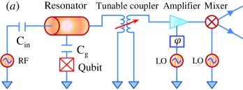
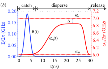
Figure 1: (a) Schematic of the measurement setup. The radio frequency (RF) source produces a microwave pulse, which populates the resonator via a small capacitor $C_{\text{in}}$. The resonator photons then interacts with a capacitively ($C_{\text{g}}$) coupled qubit. The interaction with the outgoing transmission line is controlled by a tunable coupler, which releases photons at the end of the procedure. The released field is then amplified and mixed with the local oscillator (LO) signal to be measured via homodyne detection. (b) The RF pulse $B(t)$ (blue curve) and varying qubit frequency $\omega_{\rm q}(t)$ (red curve), with approximate indication of the “catch”, “disperse”, and “release” stages. Dashed lines show the resonator frequency $\omega_{\rm r}$ and initial/final qubit frequency $\omega_{0}$; $\Delta=\omega_{\rm r}-\omega_{\rm q}$ is the detuning at the “disperse” stage.

During the “catch” stage, the initially empty resonator is driven by a microwave pulse and populated with $\sim$10 photons. At this stage the qubit is far detuned from the resonator [Fig. 1(b)], which makes the dispersive coupling negligible and allows the creation of an almost-perfect coherent state in the resonator. At the next “disperse” stage of the measurement, the qubit frequency is adiabatically tuned closer to the resonator frequency to produce a strong qubit-resonator interaction (it may even be pushed into the nonlinear regime). During this interaction, the resonator field amplitudes ($\lambda_{\rm eff}$) associated with the initial qubit states $|0\rangle$ and $|1\rangle$ rapidly accumulate additional phases and separate in the complex phase plane [see Fig. 2(a)]. Finally, at the last “release” stage of the measurement, after the qubit frequency is again detuned from the resonator, the resonator photons are released into the outgoing transmission line. The signal is subsequently amplified (by a phase-sensitive parametric amplifier) and sent to the mixer where the homodyne detection is performed.

With realistic parameters for superconducting qubit technology, we numerically show that the measurement of 30–40 ns duration can be realized with an error below $10^{-3}$, neglecting the intrinsic qubit decoherence. The latter assumption requires the qubit coherence time to be over 40 $\mu$s, which is already possible experimentally Pai11 . It is interesting that because of the interaction nonlinearity Bishop-10 ; Bla10 , increasing the microwave field beyond $\sim$10 photons only slightly reduces the measurement time. The nonlinearity also gives rise to about $\sim$50% squeezing of the microwave field (see squeezing-exp ; squeezing-Wilhelm ), which provides an order-of-magnitude reduction of the measurement error.

We consider a superconducting phase or transmon qubit capacitively coupled to a microwave resonator [Fig. 1(a)]. For simplicity we start with considering a two-level qubit (the third level will be included later) and describe the system by the Jaynes-Cummings (JC) Hamiltonian Blais-04 with a microwave drive ($\hbar=1$)

$$H =\omega_{\rm q}(t)\sigma_{+}\sigma_{-}+\omega_{\rm r}a^{{\dagger}}a+\textit{g}(a\sigma_{+}+\sigma_{-}a^{{\dagger}})$$

$$+B(t)a^{{\dagger}}e^{-i\omega t}+B^{*}(t)ae^{i\omega t},$$ (1)

where $\omega_{\rm q}(t)$ and $\omega_{\rm r}$ are, respectively, the qubit and the resonator frequencies, $\sigma_{\pm}$ are the rasing and lowering operators for the qubit, $a$ ($a^{{\dagger}}$) is the annihilation (creation) operator for the resonator photons, g (assumed real) is the qubit-resonator coupling, $B(t)$ and $\omega$ are the effective amplitude and the frequency of the microwave drive, respectively. In this work we assume $\omega=\omega_{\rm r}$.

For the microwave drive $B(t)$ and the qubit frequency $\omega_{q}(t)$ [Fig. 1(b)] we use Gaussian-smoothed step-functions: $B(t)=0.5B_{0}\{\text{Erf}[(t-t_{\rm B})/\sqrt{2}\sigma_{\rm B}]-\text{Erf}[(t-t_{\rm B}-\tau_{\rm B})/\sqrt{2}\sigma_{\text{B}}]\}$ and $\omega_{\text{q}}(t)=\omega_{0}+0.5(\Delta_{0}-\Delta)\{\text{Erf}[(t-t_{\rm q})/\sqrt{2}\sigma_{\text{q}}]-\text{Erf}[(t-t_{\rm qe})/\sqrt{2}\sigma_{\text{qe}}]\}$, where $t_{\rm B}$, $t_{\rm B}+\tau_{\rm B}$, $t_{\rm q}$, and $t_{\rm qe}$ are the centers of the front/end ramps, and $\sigma_{\rm B}$, $\sigma_{\rm q}$, and $\sigma_{\rm qe}$ are the corresponding standard deviations. In numerical simulations we use $\sigma_{\rm B}=\sigma_{\rm qe}=1$ ns (typical experimental value for a short ramp) while we use longer $\sigma_{\rm q}$ to make the qubit front ramp more adiabatic. Other fixed parameters are: $\textit{g}/2\pi=30$ MHz, $\tau_{\rm B}=1$ ns, $t_{\rm B}=3$ ns, $\omega_{\rm r}/2\pi=7$ GHz, and $\omega_{0}/2\pi=6$ GHz, so that initial/final detuning $\Delta_{0}=\omega_{\rm r}-\omega_{0}$ is 1 GHz, while the disperse-stage detuning $\Delta$ is varied. The measurement starts at $t=0$ and ends at $t_{\rm f}=t_{\rm qe}+2\sigma_{\rm qe}$ when the field is quickly released note-shape .

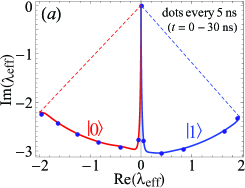
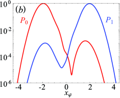
Figure 2: (a) Evolution in time of the effective field amplitude $\lambda_{\text{eff}}$ on the phase plane for initial qubit states $|0\rangle$ and $|1\rangle$, computed numerically. The dots indicate time moments $t=0$, 5, 10, 15, 20, 25, and 30 ns. (b) Corresponding probability distributions $P_{0}(x_{\varphi})$ and $P_{1}(x_{\varphi})$ for measurement (at $t=t_{\rm f}$) of the optimum quadrature $x_{\varphi}$. Side bumps of $P_{0}$ and $P_{1}$ are due to non-adiabaticity. We used $\Delta/2\pi=50$ MHz, $|\lambda_{\rm in}|^{2}=9$, $\sigma_{\rm q}=3$ ns, $t_{\rm q}=3.25$ ns, $t_{\rm qe}=30$ ns, and $t_{\rm f}=32$ ns.

Let us first consider a simple dispersive scenario at large qubit-resonator detuning, $|\Delta|\gg\textit{g}\sqrt{\overline{n}+1}$, where $\overline{n}$ is the average number of photons in the resonator. In this case, the system is described by the usual dispersive Hamiltonian Blais-04 $H_{d}=(\omega_{0}-\textit{g}^{2}/\Delta)\sigma_{z}/2+(\omega_{r}-\sigma_{z}\textit{g}^{2}/\Delta)a^{{\dagger}}a$, where $\sigma_{z}$ is the Pauli matrix. After the short “catch” stage the system is in a product state $(\alpha|0\rangle+\beta|1\rangle)|\lambda_{{\rm in}}\rangle$, where $\alpha$ and $\beta$ are the initial qubit state amplitudes and $\lambda_{{\rm in}}$ is the amplitude of the coherent resonator field, $\lambda_{\rm in}=-i\int B(t)\,dt$ (so $\overline{n}=|\lambda_{\rm in}|^{2}$). Then during the “disperse” stage the qubit-resonator state becomes entangled, $\alpha|0\rangle|\lambda_{0}(t)\rangle+\beta|1\rangle|\lambda_{1}(t)\rangle$, with $\lambda_{0}=\lambda_{\rm in}e^{-i\phi},\lambda_{1}=\lambda_{\rm in}e^{i\phi}$, and $\phi(t)=\int_{0}^{t}[\textit{g}^{2}/\Delta(t^{\prime})]dt^{\prime}$.

The distinguishablity of the two resonator states depends on their separation $|\delta\lambda|\equiv|\lambda_{1}-\lambda_{0}|=2|\lambda_{\rm in}|\sin|\phi|$ (see numerical results in Fig. 2). The released coherent states are measured via the homodyne detection using the optimal quadrature connecting $\lambda_{0}$ and $\lambda_{1}$, i.e., corresponding to the angle $\varphi=\text{arg}(\lambda_{1}-\lambda_{0})$. We rescale the measurement results to the dimensionless field quadrature ${\hat{x}}_{\varphi}=(ae^{-i\varphi}+a^{{\dagger}}e^{i\varphi})/2$, which corresponds to the $\varphi$-angle axis in the phase space of Fig. 2(a). In resolving the two coherent states, we are essentially distinguishing two Gaussian probability distributions, $P_{0}({x_{\varphi}})$ and $P_{1}({x_{\varphi}})$, centered at $\pm|\delta\lambda|\sigma_{\text{coh}}$ with $\sigma_{\text{coh}}=1/2$ being the coherent-state width (standard deviation) for both distributions. Then the measurement error has a simple form

$$E=\frac{1}{2}\int_{-\infty}^{\infty}\text{min}(P_{0},P_{1})\,d{x_{\varphi}}=\frac{1-\text{Erf}(|\delta\lambda|\sqrt{\eta/2})}{2},$$ (2)

where $\eta=\eta_{\text{\rm col}}\eta_{\text{\rm amp}}$ is the detection efficiency Kor11 , which includes the collection efficiency $\eta_{\text{col}}$ and quantum efficiency of the amplifier $\eta_{\text{amp}}$. Unless mentioned otherwise, we assume $\eta=1$, which corresponds to a quantum-limited phase-sensitive amplifier (for a phase-preserving amplifier $\eta\leq 1/2$).

In general the JC qubit-resonator interaction (Catch-Disperse-Release Readout for Superconducting Qubits) is non-linear for $|\lambda_{\rm in}|^{2}\gtrsim\overline{n}_{\rm crit}\equiv\Delta^{2}/4g^{2}$ Blais-04 and the resonator states are not coherent. The measurement error $E$ is still given by the first part of Eq. (2), while the probability distributions $P_{0,1}(x_{\varphi})$ of the measurement result for the qubit starting in either state $|0\rangle$ or $|1\rangle$ can be calculated in the following way. Assuming an instantaneous release of the field, we are essentially measuring the operator ${\hat{x}}_{\varphi}$. Therefore the probability $P(x_{\varphi})$ for the ideal detection ($\eta=1$) can be calculated by converting the Fock-space density matrix $\rho_{nm}$ describing the resonator field, into the ${{x}}_{\varphi}$-basis, thus obtaining $P({x_{\varphi}})=\sum_{nm}\psi_{n}(x_{\varphi})\rho_{nm}(t)\psi^{*}_{m}(x_{\varphi})e^{-i(n-m)\varphi}$, where $\psi_{n}(x)$ is the standard $n$th-level wave function of a harmonic oscillator. For a non-instantaneous release of the microwave field the calculation of $P({x_{\varphi}})$ is non-trivial; however, since the qubit is already essentially decoupled from the resonator, the above result for $P({x_{\varphi}})$ remains the same W-M-book for optimal time-weighting of the signal. In the case of a non-ideal detection ($\eta<1$) we should take a convolution of the ideal $P(x_{\varphi})$ with the Gaussian of width $\sqrt{\eta^{-1}-1}\,\sigma_{\text{coh}}$. Calculation of the optimum phase angle $\varphi$ minimizing the error is non-trivial in the general case. For simplicity we still use the natural choice $\varphi=\text{arg}(\lambda_{\text{eff},1}-\lambda_{\text{eff},0})$, where the effective amplitude of the resonator field Ger05 is defined by $\lambda_{\text{eff}}=\sum_{n}\sqrt{n}{\rho}_{n,n-1}$. The field density matrix ${\rho}_{nm}$ is calculated numerically using the Hamiltonian (Catch-Disperse-Release Readout for Superconducting Qubits) and then tracing over the qubit.

Extensive numerical simulations allowed us to identify two main contributions to the measurement error $E$ in our scheme. The first contribution is due to the insufficient separation of the final resonator states $|\lambda_{\rm eff,1}\rangle$ and $|\lambda_{\rm eff,0}\rangle$, as described above. However, there are two important differences from the simplified analysis: the JC nonlinearity may dramatically change $|\delta\lambda|$ and it also produces a self-developing squeezing of the resonator states in the quadrature $x_{\varphi}$, significantly decreasing the error compared with Eq. (2) (both effects are discussed in more detail later). The second contribution to the measurement error is due to the nonadiabaticity of the front ramp of the qubit frequency pulse $\omega_{q}(t)$, which leads to the population of “wrong” levels in the eigenbasis. This gives rise to the side peaks (“bumps”) in the probability distributions $P_{0,1}(x_{\varphi})$, as can be seen in Fig. 2(b) (notice their similarity to the experimental results Sid12 ; Ris12 , though the mechanism is different). During the dispersion stage these bumps move in the “wrong” direction, halting the exponential decrease in the error, and thus causing the error to saturate. The nonadiabaticity at the rear ramp of $\omega_{q}(t)$ is not important because the moving bumps do not have enough time to develop. Therefore the rear ramp can be steep, while the front ramp should be sufficiently smooth [Fig. 1(a)] to minimize the error.

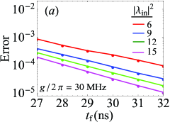
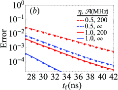
Figure 3: Optimized measurement error $E$ vs measurement time $t_{\rm f}$ (optimization is over $\Delta$, $\sigma_{\rm q}$, and $t_{\rm q}$). (a) For two-level qubit and for mean photon number $|\lambda_{\rm in}|^{2}=6,9,12$, and $15$. (b) For $|\lambda_{\rm in}|^{2}=9$ and $\eta=1$ or $1/2$ (e.g. for a phase-preserving amplifier), taking into account the qubit level $|2\rangle$ (with anharmonicity ${\mathcal{A}}/2\pi=200$ MHz) or assuming a two-level qubit ($\mathcal{A}=\infty$).

Now, let us discuss the effect of nonlinearity (when $|\lambda_{\rm in}|^{2}>\overline{n}_{\rm crit}$) on the evolution of $\lambda_{\rm eff,0}$ and $\lambda_{\rm eff,1}$ during the disperse stage. Since the RF drive is turned off, the interaction described by the Hamiltonian (Catch-Disperse-Release Readout for Superconducting Qubits) occurs only between the pairs of states $|0,n\rangle$ and $|1,n-1\rangle$ of the JC ladder. Therefore, if the front ramp of the qubit frequency pulse is adiabatic, the pairs of the JC eigenstates evolve only by accumulating their respective phases while maintaining their populations. Then for the qubit initial state $|0\rangle$, the qubit-resonator wavefunction evolves approximately as $|\psi_{0}(t)\rangle\simeq e^{-|\lambda_{\rm in}|^{2}/2}\sum_{n}(\lambda_{\rm in}^{n}/\sqrt{n!})e^{-i\phi_{0,n}(t)}|\overline{0,n}\rangle$, where the overbar denotes the (dressed) eigenstate and $\phi_{0,n}(t)=\int_{t_{\rm D}}^{t}dt^{\prime}[\sqrt{\Delta(t^{\prime})^{2}+4\textit{g}^{2}n}-\Delta(t^{\prime})]/2$ is the accumulated phase, with $t_{\rm D}=t_{\rm B}+\tau_{\rm B}/2$ being the center of the $B(t)$-pulse, which is crudely the start of the dispersion. Similarly, if the qubit starts in state $|1\rangle$ (following the ideology of Ref. RezQu , we then use $\overline{|10\rangle}$ as the initial state), the state evolves as $|\psi_{1}(t)\rangle\simeq e^{-|\lambda_{\rm in}|^{2}/2}\sum_{n}(\lambda_{\rm in}^{n}/\sqrt{n!})e^{i\phi_{1,n}(t)}|\overline{1,n}\rangle$, where $\phi_{1,n}(t)=\int_{t_{\rm D}}^{t}dt^{\prime}[\sqrt{\Delta(t^{\prime})^{2}+4\textit{g}^{2}(n+1)}-\Delta(t^{\prime})]/2$. Using the above definition of $\lambda_{\rm eff}$ and assuming $|\lambda_{\rm in}|^{2}\gg 1$ we derive an approximate formula

$$\lambda_{\text{eff},0}=\lambda_{\rm in}\exp\left[-i\int_{t_{\rm D}}^{t}\frac{\textit{g}^{2}}{\sqrt{\Delta(t^{\prime})^{2}+4\textit{g}^{2}|\lambda_{\rm in}|^{2}}}\,dt^{\prime}\right].$$ (3)

The corresponding expression for $\lambda_{\text{eff},1}$ can be obtained by replacing $-i$ with $i$ and $|\lambda_{\rm in}|^{2}$ with $|\lambda_{\rm in}|^{2}+1$. These formulas agree well with our numerical results.

Equation (3) shows that a decrease in detuning leads to an increase in the rotation speed of $\lambda_{\text{eff}}$. However, in the strongly nonlinear regime $|\lambda_{\rm in}|^{2}\gg\overline{n}_{\rm crit}$, the angular speed saturates at $d(\text{arg}(\lambda_{\text{eff,0/1}}))/dt=\mp\textit{g}/2|\lambda_{\rm in}|$. Thus, the rate at which the $\lambda_{\text{eff,1}}$ and $\lambda_{\text{eff,0}}$ separate is limited by

$$d|\delta\lambda|/dt\leq|\textit{g}|,$$ (4)

which does not depend on $|\lambda_{\rm in}|$. This means that the measurement time should not improve much with increasing the mean number of photons $|\lambda_{\rm in}|^{2}$ in the resonator, as long as it is sufficient for distinguishing the states with a desired fidelity (crudely, $|\lambda_{\rm in}|^{2}\gtrsim 7/\eta$ for $E\lesssim 10^{-4}$).

Figure 3(a) shows the results of a three-parameter optimization of the measurement error $E$ for several values of the average number of photons in the resonator, $|\lambda_{\rm in}|^{2}$ (assuming $\eta=1$). The optimization parameters are the qubit-resonator detuning $\Delta$, the width $\sigma_{q}$, and the center $t_{q}$ of the qubit front ramp. We see that for nine photons in the resonator the error of $10^{-4}$ can be achieved with 30 ns measurement duration, excluding time to release and measure the field. The optimum parameters in this case are: $\Delta/2\pi=60$ MHz, $\sigma_{q}=4.20$ ns, and $t_{q}=3.25$ ns (this is a strongly nonlinear regime: $|\lambda_{\rm in}|^{2}/\overline{n}_{\rm crit}=9$). As expected from the above discussion, increasing the mean photon number to 12 and 15 shortens the measurement time only slightly (by 1 ns and 2 ns, keeping the same error). The dashed blue curve in Fig. 3(b) shows the optimized error for $|\lambda_{\rm in}|^{2}=9$ and imperfect quantum efficiency $\eta=1/2$. As we see, the measurement time for the error level of $10^{-4}$ increases to 40 ns, while the error of $10^{-3}$ is achieved at $t_{\rm f}=32$ ns.

So far, we considered the two-level model for the qubit. However, real superconducting qubits are only slightly anharmonic oscillators, so the effect of the next excited level $|2\rangle$ is often important. It is straightforward to include the level $|2\rangle$ into the Hamiltonian (Catch-Disperse-Release Readout for Superconducting Qubits) by replacing its first term with $\omega_{\rm q}|1\rangle\langle 1|+(2\omega_{\rm q}-{\mathcal{A}})|2\rangle\langle 2|$, where ${\mathcal{A}}$ is the anharmonicity. The dispersion can then be understood as due to repulsion of three eigenstates: $\overline{|0,n\rangle}$, $\overline{|1,n-1\rangle}$, and $\overline{|2,n-2\rangle}$. As the result, $\lambda_{\rm eff,0}$ rotates on the phase plane faster than in the two-level approximation, while $\lambda_{\rm eff,1}$ rotates slower (sometimes even in the opposite direction). The Supplemental Material SM illustrates evolution of the resonator Wigner function corresponding to initial qubit states $|0\rangle$ and $|1\rangle$. In Fig. 3(b), we present the optimized error for ${\mathcal{A}}/2\pi=200$ MHz (a typical value for transmon and phase qubits), $|\lambda_{\rm in}|^{2}=9$ and $\eta=1$ (solid-red curve) or $\eta=1/2$ (dashed-red curve). An error of $10^{-3}$ can be achieved with 31 ns ($\eta=1$) and 39 ns ($\eta=1/2$) measurement durations.

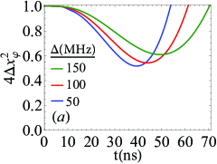
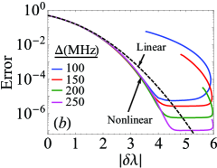
Figure 4: (a) Evolution of the quadrature squeezing (the qubit is initially in state $|0\rangle$). (b) Measurement error vs $|\delta\lambda|$ calculated numerically in the nonlinear regime (solid lines) and using the linear approximation (2) (dashed line); here the evolution stops at 98 ns. $|\lambda_{\rm in}|^{2}=9$, $\sigma_{q}=4\text{ns}$, $t_{q}=3.25$ ns.

We next discuss the self-generated quadrature squeezing of the microwave field induced by the JC nonlinearity. To quantity the degree of squeezing, we calculate the variance $\Delta x_{\varphi}^{2}=\langle x_{\varphi}^{2}\rangle-\langle x_{\varphi}\rangle^{2}=1/4+\langle a^{{\dagger}}a\rangle/2-|\langle a\rangle|^{2}/2+{\rm Re}[(\langle a^{2}\rangle-\langle a\rangle^{2})e^{-2i\varphi}]/2$. For a coherent field $\Delta x_{\varphi}^{2}=1/4$, thus the state is squeezed Ger05 when $4\Delta x_{\varphi}^{2}<1$. Figure 4(a) shows evolution of $4\Delta x_{\varphi}^{2}$ when the initial qubit state is $|0\rangle$, for $\eta=1$ and assuming a two-level qubit (a similar result is obtained for qubit initially in state $|1\rangle$). Notice that at first the field stays coherent, which is due to the linearity of the qubit-resonator interaction at large detuning. Later on, however, the interaction becomes nonlinear due to decreased detuning and leads to quadrature squeezing reaching the level of $\sim$50% for $\Delta/2\pi\lesssim 100$ MHz (see SM for the Wigner function evolution). Figure 4(b) shows the measurement error as a function of $|\delta\lambda|$ in the nonlinear regime calculated numerically (solid curves) and in the linear regime based on Eq. (2) (dashed curve). As expected, with the squeezing developing, the error becomes significantly smaller than the linear (analytical) prediction, for instance, up to a factor of 30 for $\Delta/2\pi=250$ MHz. Note also that the error shown in Fig. 4(b) saturates in spite of increasing separation $|\delta\lambda|$. This is because of the nonadiabatic error discussed above.

We do not focus on the quantum nondemolition (QND) Braginsky-Khalili property of the readout, because in the proposed implementation of the surface code Fowler-12 the measured qubits are reset, so the QNDness is not important. For the results presented in Fig. 3 the non-QND-ness (probability that the initial states $|00\rangle$ and $\overline{|10\rangle}$ are changed after the procedure) is crudely about 5%, which is mainly due to nonadiabaticity of the rear ramp. It is possible to strongly decrease the non-QND-ness by using smoother rear ramp, but it cannot be reduced below a few times $(\textit{g}/\Delta_{0})^{2}$, essentially because of the Purcell effect during the release stage. Furthermore, we do not consider the measurement-induced dephasing of the qubit, since our readout is not intended for a continuous qubit monitoring or a quantum feedback. We neglect the qubit relaxation and excitation due to “dressed dephasing” dressed-deph because its rate is smaller than the intrinsic pure dephasing, which for transmons is usually smaller than intrinsic relaxation.

In conclusion, we analyzed a fast high-fidelity readout for superconducting qubits in a cQED architecture using the controlled catch, dispersion, and release of the microwave photons. This readout uses a tunable coupler to decouple the resonator from the transmission line during the dispersion stage of the measurement, thus avoiding the Purcell effect. Our approach may also be used as a new tool to beat the standard quantum limit via self-developing field squeezing, directly measurable using the state-of-the-art parametric amplifiers.

The authors thank Farid Khalili, Konstantin Likharev, and Gerard Milburn for useful discussions. This research was funded by the Office of the Director of National Intelligence (ODNI), Intelligence Advanced Research Projects Activity (IARPA), through the Army Research Office Grant No. W911NF-10-1-0334. All statements of fact, opinion or conclusions contained herein are those of the authors and should not be construed as representing the official views or policies of IARPA, the ODNI, or the U.S. Government. We also acknowledge support from the ARO MURI Grant No. W911NF-11-1-0268.

References

- (1) K.B. Cooper, M. Steffen, R. McDermott, R.W. Simmonds, S. Oh, D.A. Hite, D.P. Pappas, and J.M. Martinis, Phys. Rev. Lett. 93, 180401 (2004).
- (2) O. Astafiev, Yu.A. Pashkin, T. Yamamoto, Y. Nakamura, and J.S. Tsai, Phys. Rev. B 69, 180507 (R) (2004).
- (3) I. Siddiqi, R. Vijay, M. Metcalfe, E. Boaknin, L. Frunzio, R.J. Schoelkopf, and M.H. Devoret, Phys. Rev. B 73, 054510 (2006).
- (4) A. Lupascu, E.F.C. Driessen, L. Roschier, C.J.P.M. Harmans, and J.E. Mooij, Phys. Rev. Lett. 96, 127003 (2006)
- (5) F. Mallet, F.R. Ong, A. Palacios-Laloy, F. Nguyen, P. Bertet, D. Vion, and D. Esteve, Nat. Phys. 5, 791 (2009).
- (6) M.D. Reed, L. DiCarlo, B. R. Johnson, L. Sun, D. I. Schuster, L. Frunzio, and R. J. Schoelkopf, Phys. Rev. Lett. 105, 173601 (2010).
- (7) A. Wallraff, D.I. Schuster, A. Blais, L. Frunzio, J. Majer, M. H. Devoret, S.M. Girvin, and R.J. Schoelkopf, Phys. Rev. Lett. 95, 060501 (2005).
- (8) A. Blais, R.-S. Huang, A. Wallraff, S.M. Girvin, and R.J. Schoelkopf, Phys. Rev. A 69, 062320 (2004).
- (9) J.E. Johnson, C. Macklin, D.H. Slichter, R. Vijay, E.B. Weingarten, J. Clarke, and I. Siddiqi, Phys. Rev. Lett. 109, 050506 (2012).
- (10) D. Riste, J.G. van Leeuwen, H.-S. Ku, K.W. Lehnert, and L. DiCarlo, Phys. Rev. Lett. 109, 050507 (2012).
- (11) N. Bergeal, F. Schackert, M. Metcalfe, R. Vijay, V.E. Manucharyan, L. Frunzio, D.E. Prober, R.J. Schoelkopf, S. M. Girvin, and M.H. Devoret, Nature (London) 465, 64 (2010).
- (12) P. Campagne-Ibarcq, E. Flurin, N. Roch, D. Darson, P. Morfin, M. Mirrahimi, M.H. Devoret, F. Mallet, and B. Huard, arXiv:1301.6095.
- (13) J. Bylander, S. Gustavsson, F. Yan, F. Yoshihara, K. Harrabi, G. Fitch, D.G. Cory, Y. Nakamura, J.-S. Tsai, and W.D. Oliver, Nat. Phys. 7, 565 (2011).
- (14) H. Paik, D.I. Schuster, L.S. Bishop, G. Kirchmair, G. Catelani, A.P. Sears, B.R. Johnson, M.J. Reagor, L. Frunzio, L.I. Glazman, S.M. Girvin, M.H. Devoret, and R.J. Schoelkopf, Phys. Rev. Lett. 107, 240501 (2011).
- (15) A.G. Fowler, M. Mariantoni, J.M. Martinis, and A.N. Cleland, Phys. Rev. A 86, 032324 (2012).
- (16) E.M. Purcell, Phys. Rev. 69, 691 (1946).
- (17) M.D. Reed, B.R. Johnson, A.A. Houck, L. DiCarlo, J.M. Chow, D.I. Schuster, L. Frunzio, and R.J. Schoelkopf, Appl. Phys. Lett. 96, 203110 (2010).
- (18) J.M. Gambetta, A.A. Houck, and A. Blais, Phys. Rev. Lett. 106, 030502 (2011).
- (19) Y. Yin, Y. Chen, D. Sank, P.J.J. O’Malley, T.C. White, R. Barends, J. Kelly, E. Lucero, M. Mariantoni, A. Megrant, C. Neill, A. Vainsencher, J. Wenner, A.N. Korotkov, A.N. Cleland, and J. M. Martinis, Phys. Rev. Lett. 110, 107001 (2013).
- (20) R.C. Bialczak, M. Ansmann, M. Hofheinz, M. Lenander, E. Lucero, M. Neeley, A.D. O’Connell, D. Sank, H. Wang, M. Weides, J. Wenner, T. Yamamoto, A. N. Cleland, and J.M. Martinis, Phys. Rev. Lett. 106, 060501 (2011).
- (21) L.S. Bishop, E. Ginossar, and S.M. Girvin, Phys. Rev. Lett. 105, 100505 (2010).
- (22) M. Boissonneault, J.M. Gambetta, and A. Blais, Phys. Rev. Lett. 105, 100504 (2010).
- (23) F. Mallet, M.A. Castellanos-Beltran, H.S. Ku, S. Glancy, E. Knill, K.D. Irwin, G.C. Hilton, L.R. Vale, and K.W. Lehnert, Phys. Rev. Lett. 106, 220502 (2011).
- (24) L.C.G. Govia, E.J. Pritchett, and F.K. Wilhelm, arXiv:1210.4042.
- (25) Actually, for we additionally use small compensating ramps at the beginning and end of the procedure to provide the exact value and to zero at and .
- (26) A.N. Korotkov, arXiv:1111.4016.
- (27) H.M. Wiseman and G.J. Milburn, Quantum Measurement and Control (Cambridge University Press, Cambridge, England, 2010), Sec. 4.7.6.
- (28) M.O. Scully and M.S. Zubairy, Quantum Optics (Cambridge University Press, Cambridge, 1997).
- (29) A. Galiautdinov, A.N. Korotkov, and J.M. Martinis, Phys. Rev. A 85, 042321 (2012).
- (30) See Supplemental Material for the Wigner function evolution.
- (31) V.B. Braginsky and F.Ya. Khalili, Quantum Measurement (Cambridge University Press, Cambridge, England, 1992).
- (32) M. Boissonneault, J.M. Gambetta, and A. Blais, Phys. Rev. A 79, 013819 (2009).