Some knots in $S^{1}\times S^{2}$ with lens space surgeries.

Abstract.

We propose a classification of knots in $S^{1}\times S^{2}$ that admit a longitudinal surgery to a lens space. Any lens space obtainable by longitudinal surgery on some knots in $S^{1}\times S^{2}$ may be obtained from a Berge-Gabai knot in a Heegaard solid torus of $S^{1}\times S^{2}$, as observed by Rasmussen. We show that there are yet two other families of knots: those that lie on the fiber of a genus one fibered knot and the ‘sporadic’ knots. All these knots in $S^{1}\times S^{2}$ are both doubly primitive and spherical braids.

This classification arose from generalizing Berge’s list of doubly primitive knots in $S^{3}$, though we also examine how one might develop it using Lisca’s embeddings of the intersection lattices of rational homology balls bounded by lens spaces as a guide. We conjecture that our knots constitute a complete list of doubly primitive knots in $S^{1}\times S^{2}$ and reduce this conjecture to classifying the homology classes of knots in lens spaces admitting a longitudinal $S^{1}\times S^{2}$ surgery.

1. Introduction

A knot $K$ in a $3$–manifold $M$ is doubly primitive if it may be embedded in a genus $2$ Heegaard surface of $M$ so that it represents a generator of each handlebody, i.e. in each handlebody there is a compressing disk that $K$ transversally intersects exactly once. With such a doubly primitive presentation, surgery on $K$ along the slope induced by the Heegaard surface yields a lens space. Berge introduced this concept of doubly primitive and provided twelve families (which partition into three broader families) of knots in $S^{3}$ that are doubly primitive [9]. The Berge Conjecture asserts that if longitudinal surgery on a knot in $S^{3}$ produces a lens space, then that knot admits a presentation as a doubly primitive knot in a genus $2$ Heegaard surface in $S^{3}$ in which the slope induced by the Heegaard surface is the surgery slope. This conjecture is regarded as implicit in [9].

This conjecture has a prehistory fueled by the classification of lens space surgeries on torus knots [34], notable examples of longitudinal lens space surgeries on non-torus knots [2, 18], the Cyclic Surgery Theorem [16], the resolution of the Knot Complement problem [23], several treatments of lens space surgeries on satellite knots [52, 12, 50], and the classification of surgeries on knots in solid tori producing solid tori [20, 21, 10] to name a few. The modern techniques of Heegaard Floer homology [41, 40] opened new approaches that reinvigorated the community’s interest and gave way to deeper insights of positivity [26], fiberedness [36], and simplicity [42, 27, 44].

One remarkable turn is Greene’s solution to the Lens Space Realization Problem [25]. Utilizing the correction terms of Heegaard Floer homology [39], Greene adapts and enhances Lisca’s lattice embedding ideas [33] to determine not only which lens spaces may be obtained by surgery on a knot in $S^{3}$ but also the homology classes of the corresponding dual knots in those lens spaces. This gives the pleasant corollary that Berge’s twelve families of doubly primitive knots in $S^{3}$ is complete.

Our present interest lies in the results of Lisca’s work [33] which, with an observation by Rasmussen [25, Section 1.5], solves the $S^{1}\times S^{2}$ version of the Lens Space Realization Problem. That is, the lens spaces which bound rational homology $4$–balls as determined by Lisca may each be obtained by longitudinal surgery on some knot in $S^{1}\times S^{2}$. (Note that if a lens space results from longitudinal surgery on a knot in $S^{1}\times S^{2}$ then it necessarily bounds a rational homology $4$–ball.) In fact, as Rasmussen observed, the standard embeddings into $S^{1}\times S^{2}$ of the Berge-Gabai knots in solid tori with longitudinal surgeries yielding solid tori suffice. Due to the uniqueness of lattice embeddings in Lisca’s situation versus the flexibility of lattice embeddings in his situation, Greene had initially conjectured that these accounted for all knots in $S^{1}\times S^{2}$ with lens space surgeries [25]. In this article we show that there are yet two more families of knots and probe their relationships with Lisca’s lattice embeddings. Indeed, here we begin a program to bring the status of the classification of knots in $S^{1}\times S^{2}$ with lens space surgeries in line with the present state of the Berge Conjecture. The main purpose of this article is to propose such a classification of knots and provide a foundation for showing our knots constitute all the doubly primitive knots in $S^{1}\times S^{2}$.

Conjecture 1.1 (Cf. Conjecture 1.9 [25]).

The knots in $S^{1}\times S^{2}$ with a longitudinal surgery producing a lens space are all doubly-primitive.

Conjecture 1.2.

A doubly-primitive knot in $S^{1}\times S^{2}$ is either a Berge-Gabai knot, a knot that embeds in the fiber of a genus one fibered knot, or a sporadic knot.

The three families of knots in Conjecture 1.2 are analogous to the three broad of families of Berge’s doubly primitive knots in $S^{3}$ and will be described below.

Section 1.6 contains some of the basic terminology and notation that will be used.

1.1. Lens spaces obtained by surgery on knots in $S^{1}\times S^{2}$

Lisca determines whether a $3$–dimensional lens space bounds a $4$–dimensional rational homology ball by studying the embeddings into the standard diagonal intersection lattice of the intersection lattice of the canonical plumbing manifold bounding that lens space, [33]. From this and that lens spaces are the double branched covers of two-bridge links, Lisca obtains a classification of which two-bridge knots in $S^{3}=\partial B^{4}$ bound smooth disks in $B^{4}$ (i.e. are slice) and which two-component two-bridge links bound a smooth disjoint union of a disk and a Möbius band in $B^{4}$. As part of doing so, he demonstrates that in the projection to $S^{3}$ these surfaces may be taken to have only ribbon singularities. Indeed he shows this by using a single banding to transform these two-bridge links into the unlink, except for two families: one for which he uses two bandings and another which was overlooked.

Via double branched covers and the Montesinos Trick, the operation of a banding lifts to the operation of a longitudinal surgery on a knot in the double branched cover of the original link. Since the double branched cover of the two component unlink is $S^{1}\times S^{2}$, Lisca’s work shows in many cases that the lens spaces bounding rational homology balls contain a knot on which longitudinal surgery produces $S^{1}\times S^{2}$. In fact, the lens spaces bounding rational homology balls are precisely those that contain a knot on which longitudinal surgery produces $S^{1}\times S^{2}$: Greene notes Rasmussen had observed that Lisca’s list of lens spaces corresponds to those that may be obtained from considering the Berge-Gabai knots in solid tori with a solid torus surgery [10, 20] as residing in a Heegaard solid torus of $S^{1}\times S^{2}$, [25, Section 1.5]. By appealing to the classification of lens spaces up to homeomorphisms we may condense the statement as follows:

Theorem 1.3 (Rasmussen via [25, Section 1.5]).

The lens space $L$ may be transformed into $S^{1}\times S^{2}$ by longitudinal surgery on a knot if and only if there are integers $m$ and $d$ such that $L$ is homeomorphic to one of the four lens spaces:

1. $L(m^{2},md+1)$ such that $\gcd(m,d)=1$;

2. $L(m^{2},md+1)$ such that $\gcd(m,d)=2$;

3. $L(m^{2},d(m-1))$ such that $d$ is odd and divides $m-1$; or

4. $L(m^{2},d(m-1))$ such that $d$ divides $2m+1$.

Note that we do permit $m$ and $d$ to be negative integers. We will augment this theorem in Theorem 1.9 with the homology classes known to contain the knots dual to these longitudinal surgeries from $S^{1}\times S^{2}$.

Since the Berge-Gabai knots in solid tori all have tunnel number one, the corresponding knots in $S^{1}\times S^{2}$ are strongly invertible. Quotienting by this strong inversion gives the analogous result for bandings of two-bridge links to the unlink (of two components).

Corollary 1.4.

The two-bridge link $K$ may be transformed into the unlink by a single banding if and only if there are integers $m$ and $d$ such that $K$ is homeomorphic to one of the four two-bridge links:

1. $K(m^{2},md+1)$ such that $\gcd(m,d)=1$;

2. $K(m^{2},md+1)$ such that $\gcd(m,d)=2$;

3. $K(m^{2},d(m-1))$ such that $d$ is odd and divides $m-1$; or

4. $K(m^{2},d(m-1))$ such that $d$ divides $2m+1$,

Remark 1.5.

By an oversight in the statement of [33, Lemma,7.2], a family of strings of integers was left out though they are produced by the proof (cf. [32, Footnote p. 247]). The use of this lemma in [33, Lemma 9.3] causes the second family in Theorem 1.3 above to be missing from [33, Definition 1.1]. Consequentially, the associated two-bridge links (these necessarily have two components) were also not shown to bound a disjoint union of a disk and a Möbius band in $B^{4}$ in that article. (Also, we have swapped the order of the last two families.)

Prompted by the uniqueness of Lisca’s lattice embeddings (Lemma 5.2) and seemingly justified by Rasmussen’s observation, Greene had originally conjectured that if a knot in $S^{1}\times S^{2}$ admits a longitudinal lens space surgery, then it arises from a Berge-Gabai knot in a Heegaard solid torus of $S^{1}\times S^{2}$, [25, Conjecture 1.8]. These knots belong to five families which we call bgi, bgii, bgiii, bgiv, and bgv and refer to collectively as the family bg of Berge-Gabai knots. We show Greene’s original conjecture is false by exhibiting two new families, gofk and spor, of knots in $S^{1}\times S^{2}$ admitting longitudinal lens space surgeries. (In fact it turns out that Yamada had previously observed the gofk family of knots admit lens space surgeries [53].) Conjecture 1.1 accordingly updates that conjecture with these two new families of doubly primitive knots in $S^{1}\times S^{2}$. Conjecture 1.2 claims that there are no other doubly primitive knots.

Theorem 1.6.

The two families gofk and spor of knots in $S^{1}\times S^{2}$ that admit a longitudinal lens space surgery, generically do not arise from Berge-Gabai knots.

Proof.

Lemma 2.2 shows that generically the knots gofk are hyperbolic and “most” have volume greater than the hyperbolic Berge-Gabai knots. Lemma 3.5 shows that, except in two cases, regardless of choice of orientations, the lens space surgery duals to the knots spor are not in the same homology class as the dual to any Berge-Gabai knot. ∎

We provide explicit demonstrations of Theorem 1.3 from two different perspectives, both of which produce the new families gofk and spor in addition to the Berge-Gabai knots.

Taking lead from Berge’s list of doubly primitive knots in $S^{3}$ [9] and the descriptions of their associated tangles [4, 5] we first obtain tangle descriptions of the Berge-Gabai knots in $S^{1}\times S^{2}$ (by way of tangle descriptions of the Berge-Gabai knots in solid tori in [6]) to provide one proof of Theorem 1.3. Then we generate families gofk and spor analogous to Berge’s families VII, VIII and IX, X, XI, XII respectively from which Theorem 1.6 falls.

Alternatively, the embeddings (given by Lisca) of the intersection lattice of the negative definite plumbing manifold bounded by a lens space suggest where an initial blow-down ought occur to cause the entire plumbing diagram to collapse to a zero framed unknot, see section 5. It turns out that the perhaps more obvious ones happen to correspond to the duals to the bg knots though the duals to the gofk also arise, Lemma 5.3. Having found the family spor by the above tangle method, we are able to identify blow-downs corresponding to the duals of these knots as well, though they do not usually cause the plumbing diagram to collapse completely. We discuss this in section 5.2.

1.2. Simple knots

A $(1,1)$–knot is a knot $K$ that admits a presentation as a $1$–bridge knot with respect to a genus $1$ Heegaard splitting of the manifold $M$ that contains it. That is, $M$ may be presented as the union of two solid tori $V_{\alpha}$ and $V_{\beta}$ in which each $K\cap V_{\alpha}$ and $K\cap V_{\beta}$ is a boundary parallel arc in the respective solid torus. We say $K$ is simple if furthermore there are meridional disks of $V_{\alpha}$ and $V_{\beta}$ whose boundaries intersect minimally in the common torus $V_{\alpha}\cap V_{\beta}$ in $M$ such that each arc $K\cap V_{\alpha}$ and $K\cap V_{\beta}$ is disjoint from these meridional disks. One may show there is a unique (oriented) simple knot in each (torsion) homology class of a lens space. Let us write $K(p,q,k)$ for the simple knot in $M=L(p,q)$ oriented so that it represents the homology class $k\mu$ where (for a choice of orientation) $\mu$ is the homology class of the core curve of one of the Heegaard solid tori and $q\mu$ is the homology class of the other. Observe that trivial knots are simple knots and, as such, permits both $S^{3}$ and $S^{1}\times S^{2}$ to have a simple knot. There are no simple knots representing the non-torsion homology classes of $S^{1}\times S^{2}$. Non-trivial simple knots have also been called grid number one knots, e.g. in [8, 7] among others.

The Homma-Ochiai-Takahashi recognition algorithm for $S^{3}$ among genus $2$ Heegaard diagrams [29] says that a genus $2$ Heegaard diagram of $S^{3}$ is either the standard one or contains what is called a wave, see Section 4. A wave in a Heegaard diagram indicates the existence of a handle slide that will produce a new Heegaard diagram for the same manifold with fewer crossings. As employed by Berge [9], the existence of waves ultimately tells us that any $(1,1)$–knot in a lens space with a longitudinal $S^{3}$ surgery is isotopic to a simple knot. As the dual to a doubly primitive knot is necessarily a $(1,1)$–knot, it follows that the dual to a doubly primitive knot in $S^{3}$ is a simple knot in the resulting lens space.

Negami-Okita’s study of reductions of diagrams of $3$–bridge links gives insights to the existence of wave moves on genus $2$ Heegaard diagrams.

Theorem 1.7 (Negami-Okita [35]).

Every Heegaard diagram of genus $2$ for $S^{1}\times S^{2}\#L(p,q)$ may be transformed into one of the standard ones by a finite sequence of wave moves.

Here, a standard genus $2$ Heegaard diagram $H=(\Sigma,\{\alpha_{1},\alpha_{2}\},\{\beta_{1},\beta_{2}\})$ for $S^{1}\times S^{2}\#L(p,q)$ is one for which $\alpha_{1}$ and $\beta_{1}$ are parallel and disjoint from $\alpha_{2}\cup\beta_{2}$, and $\alpha_{2}\cap\beta_{2}$ consists of exactly $p$ points. If $p\neq 1$, then the standard diagrams are not unique. For our case at hand however, $p=1$ and the standard diagram is unique (up to homeomorphism). This enables a proof of a result analogous to Berge’s.

Theorem 1.8.

1. A $(1,1)$–knot in a lens space with a longitudinal $S^{1}\times S^{2}$ surgery is a simple knot.

2. The dual to a doubly primitive knot in $S^{1}\times S^{2}$ is a simple knot in the corresponding lens space.

A proof of this follows similarly to Berge’s proof for doubly primitive knots in $S^{3}$ and their duals, though there is a technical issue one ought mind. We will highlight this as we sketch the argument of a more general result in section 4 following Saito’s treatment of Berge’s work in the appendix of [46].

1.3. The known knots in lens spaces with longitudinal $S^{1}\times S^{2}$ surgeries.

Since our knots in families bg, gofk, and spor are all doubly primitive, then by Theorem 1.8 their lens space surgery duals are simple knots. In particular, this means these duals are all at most $1$–bridge with respect to the Heegaard torus of the lens space, and thus they admit a nice presentation in terms of linear chain link surgery descriptions of the lens space. This surgery description (which we first obtained by simplifying ones suggested by the lattice embeddings) facilitates the calculation of the homology classes of these dual knots and hence their descriptions as simple knots.

Given the lens space $L(p,q)$, let $\mu$ and $\mu^{\prime}$ be homology classes of the core curves of the Heegaard solid tori oriented so that $\mu^{\prime}=q\mu$. The homology class of a knot in $L(p,q)$ is given as its multiple of $\mu$.

Theorem 1.9.

The lens spaces $L(m^{2},q)$ of Theorem 1.3 may be obtained by longitudinal surgeries on the following simple knots $K=K(m^{2},q,k)$ listed below.

1. $q=md+1$ such that $\gcd(m,d)=1$ and either

   • $k=\pm m$ so that $K$ is the dual to a bgi knot or

   • $k=\pm dm$ so that $K$ is the dual to a gofk knot;

2. $q=md+1$ such that $\gcd(m,d)=2$ and

   • $k=\pm m$ so that $K$ is the dual to a bgii knot;

3. $q=d(m-1)$ such that $d$ is odd and divides $m-1$ and either

   • $k=\pm dm$ so that $K$ is the dual to a bgiii knot,

   • $k=\pm m$ so that $K$ is the dual to a bgv knot, or

   • $k=\pm 2m=\pm 4m$ so that $K$ is the dual to a spor knot if $m=1-2d$; or

4. $q=d(m-1)$ such that $d$ divides $2m+1$ and

   • $k=\pm m$ or $k=\pm dm$ so that $K$ (in each case) is the dual to a bgiv knot.

Together Conjectures 1.1 and 1.2 assert that Theorem 1.9 gives a complete list of knots in lens spaces with a longitudinal $S^{1}\times S^{2}$ surgery. The possible lens spaces containing such knots are given in Theorem 1.3, but the homology classes of these knots have not yet been determined.

Conjecture 1.10.

If a knot in a lens space $L$ represents the homology class $\kappa\in H_{1}(L)$ and admits a longitudinal surgery to $S^{1}\times S^{2}$ then, up to homeomorphism, $L=L(m^{2},q)$ and $\kappa=k\mu$ are as in some case of Theorem 1.9.

Remark 1.11.

We are informed that Cebanu has established this conjecture for $L$ as in the first two cases of Theorem 1.9, i.e. when $L\cong L(m^{2},md+1)$ and $\gcd(m,d)=1,2$ [15].

Remark 1.12.

While Greene’s work on lattice embeddings produced a classification of the homology classes of knots in lens spaces with a longitudinal $S^{3}$ surgery [25], Lisca’s work on lattice embeddings does not appear to produce information about the classification of homology classes of knots in lens spaces with longitudinal $S^{1}\times S^{2}$ surgeries [33]. Nevertheless we examine a manner in which Lisca’s lattice embeddings suggest knots in lens spaces with such surgeries in section 5.

Remark 1.13.

In [17], the authors classify the strongly invertible knots in $L((2n-1)^{2},2n)$ with longitudinal $S^{1}\times S^{2}$ surgeries. These belong to the first case of Theorem 1.9 with $m=2n-1$ and $d=1$. The knots are bgi knots and may also be realized as gofk knots.

Theorem 1.14.

Conjecture 1.10 implies Conjecture 1.2.

That is, confirming the list of homology classes of knots in lens spaces admitting a longitudinal $S^{1}\times S^{2}$ surgery will confirm that the families bg, gofk, spor together constitute all the doubly primitive knots in $S^{1}\times S^{2}$.

Proof.

Because there is a unique simple knot for each homology class in a lens space, this theorem follows from Theorem 1.8. ∎

Remark 1.15.

Indeed, Conjecture 1.1 may be rephrased as saying if a knot $K$ in a lens space $L$ admits a longitudinal $S^{1}\times S^{2}$ surgery, then up to homeomorphism $L=L(p,q)$ and $[K]=\kappa=k\mu$ in some case of Theorem 1.9 and moreover $K=K(p,q,k)$.

1.4. Fibered knots and spherical braids

Ni shows that knots in $S^{3}$ with a lens space surgery have fibered exterior [36]. One expects the same to be true for any knot in $S^{1}\times S^{2}$ with a lens space surgery. Using knot Floer Homology, Cebanu shows this is indeed the case.

Theorem 1.16 (Cebanu [15]).

A knot in $S^{1}\times S^{2}$ with a longitudinal lens space surgery has fibered exterior.

Prior to learning of Cebanu’s results, we had confirmed this for all our knots by showing they are spherical braids. This is done in section 7. A link in $S^{1}\times S^{2}$ is a (closed) spherical braid if it is transverse to $\{\theta\}\times S^{2}$ for each $\theta\in S^{1}$.

Theorem 1.17.

In $S^{1}\times S^{2}$, the knots in families bg, gofk, and spor are all isotopic to spherical braids.

Braiding characterizes fiberedness for non-null homologous knots in $S^{1}\times S^{2}$.

Lemma 1.18.

A non-null homologous knot in $S^{1}\times S^{2}$ has fibered exterior if and only if it is isotopic to a spherical braid.

Proof.

If $K$ is a spherical braid, then the punctured spheres $(\{\theta\}\times S^{2})-N(K)$ for $\theta\in S^{1}$ fiber the exterior of $K$. Let $X(K)=S^{1}\times S^{2}-N(K)$ denote the exterior of a knot $K$ in $S^{1}\times S^{2}$. If $K$ is a non-null homologous in $S^{1}\times S^{2}$, then the kernel of the map $H_{1}(\partial X(K))\to H_{1}(X(K),\partial X(K))$ induced by inclusion is generated by a multiple of the meridian of $K$. Hence if $X(K)$ is fibered, then the boundary of a fiber is a collection of coherently oriented meridional curves. Therefore the trivial (meridional) filling of $X(K)$ which returns $S^{1}\times S^{2}$ must also produce a fibration over $S^{1}$ by closed surfaces, the capped off fibers of $X(K)$. Hence the fibers of $X(K)$ must be punctured spheres, and so $K$ is isotopic to a spherical braid. ∎

Remark 1.19.

Together Theorem 1.16 and Lemma 1.18 suggest the study of surgery on spherical braids.

One may care to compare these results with Gabai’s resolution of Property R [19]: The only knot in $S^{1}\times S^{2}$ with a surgery yielding $S^{3}$ is a fiber $S^{1}\times\ast$.

1.5. Geometries of knots and lens space surgeries

For completeness, here we address the classification of lens space Dehn surgeries on non-hyperbolic knots in $S^{1}\times S^{2}$.

We say a knot $K$ in a $3$–manifold $M$ is either spherical, toroidal, Seifert fibered, or hyperbolic if its exterior $M-N(K)$ contains an essential embedded sphere, contains an essential embedded torus, admits a Seifert fibration, or is hyperbolic respectively. By Geometrization for Haken manifolds, a knot $K$ in $S^{1}\times S^{2}$ is (at least) one of these. By the Cyclic Surgery Theorem [16], if a non-trivial knot $K$ admits a non-trivial lens space surgery, then either the surgery is longitudinal or $K$ is Seifert fibered.

If $K$ is spherical, then one may find a separating essential sphere in the exterior of $K$. Since $S^{1}\times S^{2}$ is irreducible, $K$ is contained in a ball. Therefore $K$ only admits a lens space surgery (in fact an $S^{1}\times S^{2}$ surgery) if $K$ is the trivial knot, [19, 24].

If $K$ is Seifert fibered then $K$ is a torus knot. This follows from the classification of generalized Seifert fibrations of $S^{1}\times S^{2}$, [30]. Note that the exceptional generalized fiber of $M(-1;(0,1))$ is a regular fiber of $M(0;(2,1),(2,-1))$, and its exterior is homeomorphic to both the twisted circle bundle over the Möbius band and the twisted interval bundle over the Klein bottle. For relatively prime integers $p,q$ with $p\geq 0$, we define a $(p,q)$–torus knot $T_{p,q}$ in $S^{1}\times S^{2}$ to be a regular fiber of the generalized Seifert fibration $M(0;(p,q),(p,-q))$. (The exceptional fibers may be identified with $S^{1}\times\mbox{ \sc n}$ and $S^{1}\times\mbox{ \sc s}$ for antipodal points $\mbox{ \sc n},\mbox{ \sc s}\in S^{2}$.) Equivalently, we may regard $T_{p,q}$ as a curve on $\partial N(S^{1}\times\ast)$, $\ast\in S^{2}$, that is homologous to $q\mu+p\lambda\in H_{1}(\partial N(S^{1}\times\ast))$ for meridian-longitude classes $\mu,\lambda$ and an appropriate choice of orientation on $T_{p,q}$. Observe $[T_{p,q}]=p[S^{1}\times\ast]\in H_{1}(S^{1}\times S^{2})$ and $T_{p,q}=T_{p,q+Np}$ for any integer $N$. Following [34, 22] (though note that on the boundary of a solid torus, a $(p,q)$ curve for them is a $(q,p)$ curve for us) any non-trivial lens space surgery on a $(p,q)$–torus knot with $p\geq 2$ has surgery slope $1/n$, taken with respect to the framing induced by the Heegaard torus, and yields the lens space $L(np^{2},npq+1)$.

If $K$ is toroidal and admits a non-trivial lens space surgery then the proof in [12] applies basically unaltered (because Seifert fibered knots in $S^{1}\times S^{2}$ are torus knots and lens spaces are atoroidal) to show $K$ must be a $(2,\pm 1)$–cable of a torus knot, where the cable is taken with respect to the framing on the torus knot induced by the Heegaard torus. If $K$ is the $(2,\pm 1)$–cable of the $(p,q)$–torus knot, then $\pm 1$ surgery on $K$ with respect to its framing as a cable is equivalent to $\pm 1/4$ surgery on the $(p,q)$–torus knot and thus yields $L(4p^{2},4pq\pm 1)$ or its mirror.

Hence we have:

Theorem 1.20.

A non-hyperbolic knot in $S^{1}\times S^{2}$ with a non-trivial lens space surgery is either a $(p,q)$–torus knot or a $(2,\pm 1)$–cable of a $(p,q)$–torus knot.

Because the $(2,1)$–torus knot in $S^{1}\times S^{2}$ contains an essential Klein bottle in its exterior, it is toroidal.

Corollary 1.21.

• The smallest order lens space obtained by surgery on a toroidal knot in $S^{1}\times S^{2}$ is homeomorphic to $L(4,1)$. The surgery dual is the simple knot $K(4,1,2)$.

• The smallest order lens space obtained by surgery on a non-torus, toroidal knot in $S^{1}\times S^{2}$ is homeomorphic to $L(16,9)$. The surgery dual is the (unoriented) simple knot $K(16,9,4)$.

(The orientation of a knot has no bearing upon its surgeries. Ignoring orientations, $K(16,9,4)$ is equivalent to $K(16,9,12)$. The simple knot $K(4,1,2)$ is isotopic to its own orientation reverse.)

Bleiler-Litherland conjecture that the smallest order lens space obtained by surgery on a hyperbolic knot in $S^{3}$ is homeomorphic to $L(18,5)$ [12]. Among our list of doubly primitive knots in $S^{1}\times S^{2}$, up to homeomorphism, we find three hyperbolic knots of order $5$ in families bgiii, bgv, and gofk with integral lens space surgeries; all the doubly primitive knots with smaller order are non-hyperbolic.

Conjecture 1.22.

Up to homeomorphism, $L(25,7)$ and $L(25,9)$ are the smallest order lens spaces obtained by surgery on a hyperbolic knot in $S^{1}\times S^{2}$. Moreover, the surgeries occur on the knots shown in Figure 1. From left to right, their surgery duals are the (unoriented) simple knots $K(25,7,5)$, $K(25,7,10)$, and $K(25,9,10)$ respectively.

Remark 1.23.

The knots on the right and left of Figure 1 are actually isotopic. Kadokami-Yamada show that among the non-torus gofk knots this is the only one (up to homeomorphism) that admits two non-trivial lens space surgeries [31]. Along these lines, Berge shows there is a unique hyperbolic knot in the solid torus with two non-trivial lens space surgeries [10], and this gives rise to a single bgiv knot (up to homeomoprhism) having surgeries to both orientations of $L(49,18)$ [11].

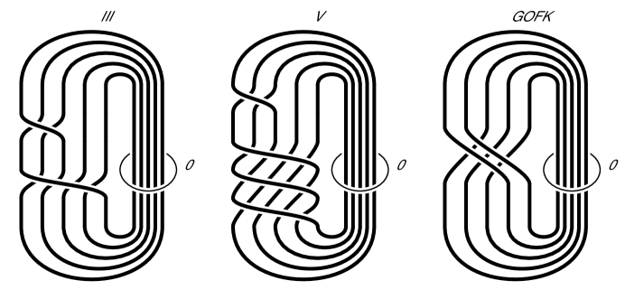
Figure 1.

1.6. Basic definitions and some notation

1.6.1. Dehn surgery

Consider a knot $K$ in a closed $3$–manifold $M$ with regular solid torus neighborhood $N(K)$. The isotopy classes of essential simple closed curves on $\partial N(K)\cong\partial(M-N(K))$ are called slopes. The meridian of $K$ is the slope that bounds a disk in $N(K)$ while the slopes that algebraically intersect the meridian once (and hence are isotopic to $K$ in $N(K)$) are longitudes. Given a slope $\gamma$, the manifold obtained by removing the solid torus $N(K)$ from $M$ and attaching another solid torus so that $\gamma$ is its meridian is the result of $\gamma$–Dehn surgery on $K$. The core of the attached solid torus is a new knot in the resulting manifold and is the surgery dual to $K$. If $\gamma$ is a longitude, then $\gamma$–Dehn surgery is a longitudinal surgery or simply a surgery. Fixing a choice of longitude and orienting both the meridian and this longitude so that they represent homology classes $\mu$ and $\lambda$ in $H_{1}(\partial N(K))$ with $\mu\cdot\lambda=+1$ enables a parametrization associating the slope $\gamma$ to the extended rational number $\frac{p}{q}\in\mathbb{Q}\cup\{1/0\}$, $\gcd(p,q)=1$, if for some orientation $[\gamma]=p\lambda+q\mu$. Then $\gamma$–Dehn surgery may also be denoted $\frac{p}{q}$–Dehn surgery. Consequentially longitudinal surgery is also called integral surgery.

1.6.2. Tangles and bandings

The knot $K$ in $M$ is said to be strongly invertible if there is an involution $u$ on $M$ that set-wise fixes $K$ and whose fixed set intersects $K$ exactly twice, and the involution is said to be a strong involution. The quotient of $M$ by $u$ is a $3$–manifold $M/\sim$, where $x\sim u(x)$, in which the fixed set of $u$ descends to a link $J$ and the knot $K$ descends to an embedded arc $\alpha$ such that $J\cap\alpha=\partial\alpha$. A small ball neighborhood $B=N(\alpha)$ of $\alpha$ intersects $J$ in a pair of arcs $t$ so that $(B,t)$ is a rational tangle, i.e. a tangle in a ball homeomorphic to $(D^{2}\times I,\{\pm\frac{1}{2}\}\times I)$ where $D^{2}$ is the unit disk in the complex plane and $I$ is the interval $[-1,1]$. The solid torus neighborhood $N(K)$ of $K$ may be chosen so that the image of its quotient under $u$ is $B$, and equivalently so that it is the double cover of $B$ branched along $t$. The Montesinos Trick refers to the correspondence through branched double covers and quotients by strong involutions between replacing the rational tangle $(B,t)$ with another and Dehn surgery on $K$. In particular, a banding of $J$ along the arc $\alpha$ corresponds to longitudinal surgery on $K$. A banding of $J$ is the act of embedding of a rectangle $I\times I$ in $M/\sim$ to meet $J$ in the pair of opposite edges $I\times\partial I$ and exchanging those sub-arcs of $J$ for the other pair of opposite edges $\partial I\times I$. The banding occurs along an arc $\alpha=\{0\}\times I$ and the banding produces the dual arc $I\times\{0\}$. Figure 3 illustrates the banding operation and both its framed arc and literal band depictions that we use in this article. Figure 3 shows how a rectangular box labeled with an integer $n$ denotes a sequence of $|n|$ twists in the longer direction. The twists are right handed if $n>0$ and left handed if $n<0$. To highlight cancellations, a pair of twist boxes will be colored the same if their labels have opposite sign.

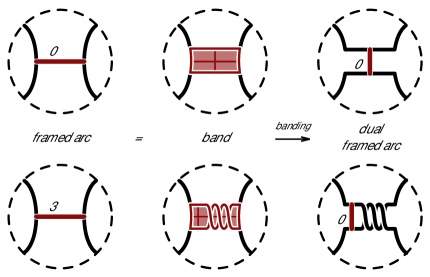
Figure 2.

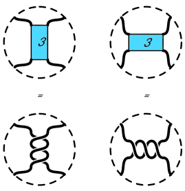
Figure 3.

1.6.3. Lens spaces, two bridge links, plumbing manifolds

The lens space $L(p,q)$ is defined as the result of $-p/q$–Dehn surgery on the unknot in $S^{3}$. The lens space $L(p,q)$ may be obtained by surgery on the linear chain link as shown at the top of Figure 4 with integral surgery coefficients $-a_{1},\dots,-a_{n}$ that are the negatives of the coefficients of a continued fraction expansion

$$\frac{p}{q}=[a_{1},\dots,a_{n}]^{-}=a_{1}-\cfrac{1}{a_{2}-\cfrac{1}{\quad\overset{\ddots}{a_{n-1}-\cfrac{1}{a_{n}}}}}.$$

The picture of this chain link also shows the axis of a strong involution $u$ that extends through the surgery to an involution of the lens space. The quotient of this involution of the lens space, via the involution of this surgery diagram, is $S^{3}$ in which the axis descends to the two-bridge link $K(p,q)$ with the diagram $L(-a_{1},\dots,-a_{n})$ as shown at the bottom of Figure 4. The orientation preserving double cover of $S^{3}$ branched over $K(p,q)$ is the lens space $L(p,q)$. Observe that the two-component unlink is $K(0,1)$, $0/1=[0]^{-}$, and we regard $S^{1}\times S^{2}$ as the lens space $L(0,1)$.

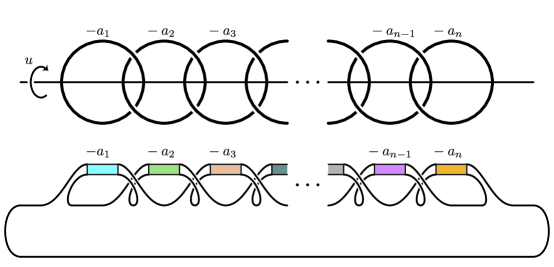
Figure 4.

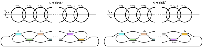
Figure 5.

From a $4$–manifold perspective, the top of Figure 4 is a Kirby diagram for a plumbing manifold whose boundary is $L(p,q)$. By an orientation preserving homeomorphism, we may take $p>q>0$ and restrict the continued fraction coefficients to be integers $a_{i}\geq 2$ so that $L(p,q)$ is the oriented boundary of the negative definite plumbing manifold $P(p,q)$ associated to the tuple $(-a_{1},\dots,-a_{n})$.

Figure 5 shows alternative (and isotopic) versions of this chain link and two-bridge link diagrams for the two cases of $n$ even and $n$ odd.

1.7. Acknowledgements

The authors would like to thank John Berge, Radu Cebanu, and Joshua Greene.

This work is partially supported by grant #209184 to Kenneth L. Baker from the Simons Foundation, by the Spanish GEOR MTM2011-22435 to Ana G. Lecuona, and EPSRC grants G039585/1 and H031367/1 to Dorothy Buck.

2. Generalizing Berge’s doubly primitive knots

Berge describes twelve families of doubly primitive knots in $S^{3}$, [9]. Greene confirms that this list is complete, [25]. The first author gives surgery descriptions of these knots and tangle descriptions of the quotients by their strong involutions, [4, 5]. (These knots admit unique strong involutions, [51].)

We partition Berge’s twelve families into three broader families: The Berge-Gabai knots, family bg, arising from knots in solid tori with longitudinal surgeries producing solid tori. The knots that embed in the fiber of a genus one fibered knot (the figure eight knot or a trefoil), family gofk. The so-called sporadic knots, family spor, which may be seen to embed in a genus one Seifert surface of a banding of a $(2,\pm 1)$–cable of a trefoil. (The framing of this cabling is with respect to the Heegaard torus containing the trefoil.)

Here, we generalize these three families of doubly primitive knots in $S^{3}$ to obtain three analogous families of doubly primitive knots in $S^{1}\times S^{2}$ that we also call bg, gofk, and spor. We provide explicit descriptions of these using tangle descriptions.

2.1. The bg knots

Let us say a strong involution of a knot in a solid torus is an involution of a solid torus whose fixed set is two properly embedded arcs such that the knot intersects this fixed set twice and is invariant under the involution. The quotient of the pair of the solid torus and fixed set under this involution is a rational tangle $(B,t)$ where $B$ is a $3$–ball and $t$ is a pair of properly embedded arcs together isotopic into $\partial B$. The image of the knot in this quotient is an arc $\alpha$ embedded in $B$ with $\partial\alpha=\alpha\cap t$. A knot with a strong involution is strongly invertible.

The Berge-Gabai knots in solid tori are all strongly invertible as evidenced by them being $1$–bridge braids (or torus knots) and hence tunnel number $1$. We say an arc $\alpha$ in a rational tangle is a Berge-Gabai arc if it is the image of a Berge-Gabai knot under the quotient by a strong involution. By virtue of the Berge-Gabai knots admitting longitudinal solid torus surgeries, there are bandings along these arcs that produce rational tangles. The dual arcs to these bandings in the new rational tangles are also Berge-Gabai arcs. Using these we obtain a proof of Theorem 1.3 along the lines of Rasmussen’s observation.

Tangle Proof of Theorem 1.3.

Doubling a rational tangle (by gluing it to its mirror) produces the two-component unlink $K(0,1)$. Therefore, if $(B,t)$ is a rational tangle and $\alpha$ is a Berge-Gabai arc in $(B,t)$ along which a banding produces the rational tangle $(B,t^{\prime})$, then banding the double $(B,t)\cup-(B,t)=(S^{3},K(0,1))$ along $\alpha$ produces the two-bridge link $(B,t^{\prime})\cup-(B,t)$.

In [6], descriptions of the Berge-Gabai arcs are derived from the quotient tangle descriptions in [5] of the knots in Berge’s doubly primitive families I – VI [9]. As done in [6], one may then explicitly observe that family VI is contained within family V, and (with mirroring) family V is dual to family III. Families I, II, and IV are each self-dual. (One family of Berge-Gabai arcs is dual to another if the arc dual to the banding along any arc in the first family, together with the resulting tangle, may be isotoped while fixing the boundary of the tangle into the form of a member of the second family.) It is also shown in [6] that these knots in solid tori admit a unique strong involution in which the solid torus quotients to a ball, and hence up to homeomorphism there is a unique arc in a rational tangle corresponding to each Berge-Gabai knot in the solid torus. The resulting classification of bandings between rational tangles up to homeomorphism from [6] is shown in Figure 6. Figures 7, 8, and 9 show the result of doubling these families (with their duals) to obtain $K(0,1)$ and then banding along a Berge-Gabai arc to obtain a two-bridge link. Observe that the two-bridge links produced by the dual pairs in families III and V in Figures 7 are equivalent as are the two-bridge links produced by the dual pairs in family IV. For the purposes of proving Theorem 1.3 only one among each of these dual pairs is required.

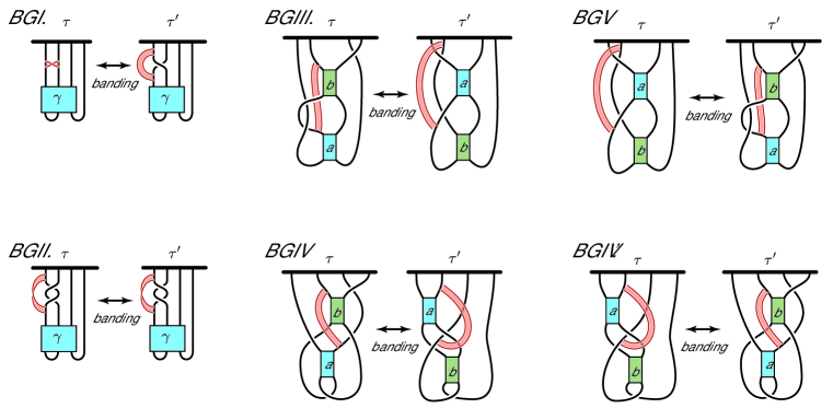
Figure 6. The bandings between rational tangles up to homeomorphism, corresponding to the double branched covers of the Berge-Gabai knots in solid tori. For bgi and bgii $\gamma$ is a $3$–braid.

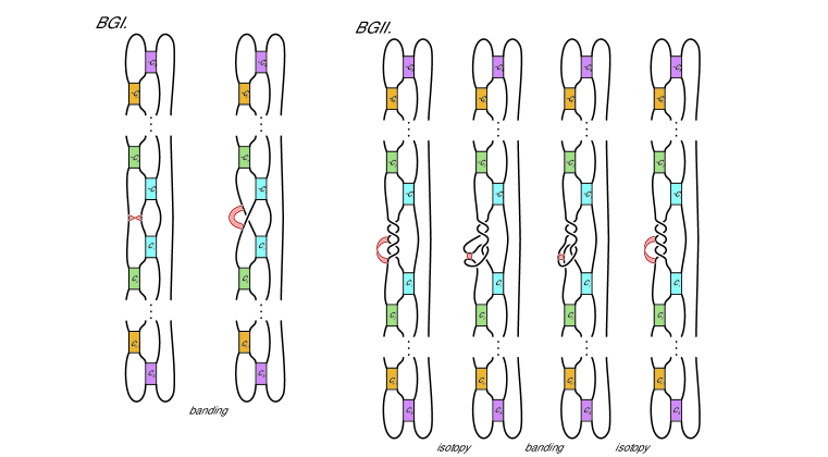
Figure 7. Left, a banding from the unlink to $K(p,q)$ where $\frac{p}{q}=[c_{k},\dots,c_{1},-1,-c_{1},\dots,-c_{k}]^{-}$ corresponding to family bgi. Right, a banding from the unlink to $K(p,q)$ where $\frac{p}{q}=[c_{k},\dots,c_{1},4,-c_{1},\dots,-c_{k}]^{-}$ corresponding to family bgii.

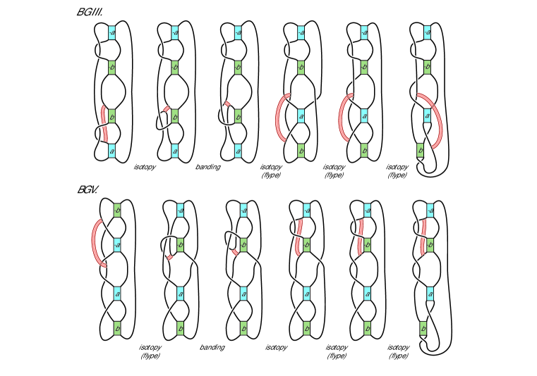
Figure 8. Two bandings between the unlink and $K(p,q)$ where $\frac{p}{q}=[a,2,b,2,-a+1,-b+1]^{-}$ corresponding to families bgiii and bgv.

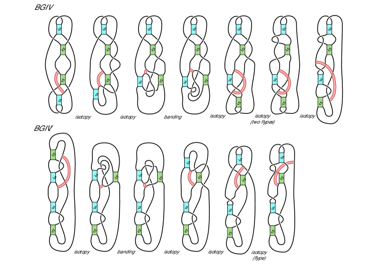
Figure 9. Two bandings between the unlink and $K(p,q)$ where $\frac{p}{q}=[a-1,-2,b,-a+1,2,-b]^{-}$ both corresponding to family bgiv.

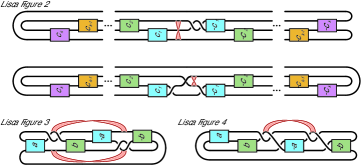
Figure 10.

We now observe that the two-bridge links produced match with those of Lisca’s Section 8 [33]. He shows that up to homeomorphism these links may be presented as in the first of one of his Figure 2, Figure 3, or Figure 4. We redraw these three in Figure 10 for the reader’s convenience, isotoping his Figure 2. In each of his Figure 2 and Figure 4 Lisca exhibits a single banding as shown in our Figure 10 that transforms those two-bridge links to the unlink. In his Figure 3 he uses two bandings as also shown in our Figure 10. As one may now observe, the two bridge links of Lisca’s Figures 2,3,4 correspond (with mirroring and reparametrizations as needed) to those produced respectively in families I, IV, III of Figures 7, 9, and 8. Note that family II produces two-bridge links not accounted for in Lisca’s pictures. Nevertheless the corresponding lens spaces are accounted for in his proof of [33, Lemma 7.2], as discussed in Remark 1.5. ∎

Remark 2.1.

In $S^{1}\times S^{2}$, as in $S^{3}$, family I consists of the torus knots while family II consists of the $(2,\pm 1)$–cables of torus knots. (This cable is taken with respect to the framing induced by the Heegaard torus containing the torus knot.) Families III, IV, and V contain hyperbolic knots.

2.2. The gofk knots

Conjecture 1.8 of [25] proposes that the knot surgeries corresponding to the double branched covers of the above bandings are, up to homeomorphisms, the only way that integral surgery on a knot in $S^{1}\times S^{2}$ may yield a lens space. However since $S^{1}\times S^{2}$ contains a genus one fibered knot, we may form the family gofk of knots that embed in the fiber of genus one fibered knots in $S^{1}\times S^{2}$ and then mimic [4] to produce our first infinite family of counterexamples.

The annulus together with the identity monodromy gives an open book for $S^{1}\times S^{2}$. Plumbing on a positive Hopf band along a spanning arc produces a once-punctured torus open book, i.e. a (null-homologous) genus one fibered knot. One may show (e.g. [3]) that this and its mirror are the only two genus one fibered knots in $S^{1}\times S^{2}$. Any essential simple closed curve in one of these fibers is then a doubly primitive knot in $S^{1}\times S^{2}$ and thus admits a lens space surgery along the slope of its page framing. We call the family of these essential simple closed curves the gofk. These knots are analogous to the knots in Berge’s families VII and VIII, [9]. Yamada had previously developed this family of knots with these lens space surgeries [53], though he constructs them from a different viewpoint.

Lemma 2.2.

There are gofk knots that are not Berge-Gabai knots. Moreover the gofk knots contain hyperbolic knots of arbitrarily large volume.

Proof.

Following [4] each gofk knot admits a surgery description on the Minimally Twisted $2n+1$ Chain link (the MT$(2n+1)$C for short) for some $n\in\mathbb{Z}$. Furthermore, for each positive integer $n$ and any value $N$, there is a doubly primitive knot on a once-punctured torus page of this open book with a surgery description on the MT$(2n+1)$C whose surgery coefficients all have magnitude greater than $N$. Therefore, as in [4], since MT$(2n+1)$C is hyperbolic for $n\geq 2$ we may conclude using Thurston’s Hyperbolic Dehn Surgery Theorem [49] and the lower bound on a hyperbolic manifold with $n$ cusps [1] that the set of volume of hyperbolic knots on this once-punctured torus page is unbounded. The Berge-Gabai knots in $S^{1}\times S^{2}$ of [25, Conjecture 1.8] however all admit surgery descriptions on the MT5C (as apparent from [5]) and thus have volume less than $\operatorname{vol}(MT5C)<11$. ∎

Any genus one fibered knot may be viewed as the lift of the braid axis in the double cover of $S^{3}$ branched over a closed $3$–braid. This enables a pleasant interpretation of the gofk knots and their lens space surgeries as corresponding to bandings from a closed $3$–braid presentation of the unlink to two-bridge links. Because Lisca’s list of two-bridge links that admit bandings to the unlink is complete, these bandings must give different bandings to the unlink for some (in a sense, most) two-bridge links. Indeed Figure 11 shows the two different bandings between the unlink and a two-bridge link corresponding to the gofk knots on the left and bgi knots on the right.

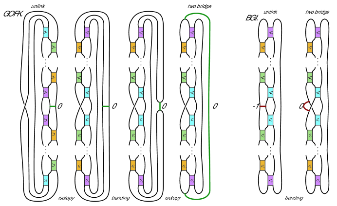
Figure 11. Left, a banding from the unlink to a two-bridge link corresponding to family gofk. Right, a banding from the unlink to the same two-bridge link corresponding to family bgi.

2.3. The spor knots

Berge’s families IX–XII of doubly primitive knots in $S^{3}$ condense to two families and are collectively referred to as the sporadic knots. In the double branched cover, the family of blue arcs ($n\in\mathbb{Z}$) in the second link of Figure 12 lifts to the analogous sporadic knots in $S^{1}\times S^{2}$, the $S^{1}\times S^{2}$–spor knots. (As one may confirm by examining the tangle descriptions in [5], Berge’s two sporadic knot families are obtained by placing $-3$ instead of $-2$ twists in either the top or bottom dashed oval, but not both.) This second link is the two-component unlink as illustrated by the subsequent isotopies. The link at the beginning of Figure 12 results from banding as shown. It is a two-bridge link and coincides with the two bridge link in family III of Figure 8 with $a=n$ and $b=-1$ and, after mirroring, with the two-bridge link of Lisca’s Figure 4 in our Figure 10 with $a=2$ and $b=-n+1$. In Section 3 we show these knots are generically distinct from the Berge-Gabai knots by examining the homology classes of the corresponding knots in the lens spaces.

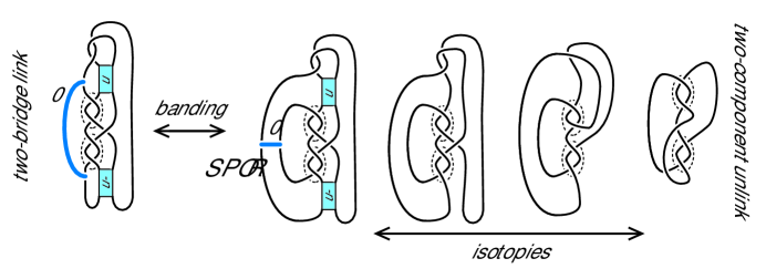
Figure 12. A banding between a two-bridge link and the unlink corresponding to the sporadic family of knots. Replace either of the $-2$ twists in the dashed ovals, but not both, with $-3$ twists to obtain bandings corresponding to Berge’s families of sporadic knots in $S^{3}$.

3. Homology classes of the dual knots in lens spaces

Figure 13 gives, up to homeomorphism, strongly invertible surgery descriptions of the lens space duals to the bg, gofk, and spor knots with their $S^{1}\times S^{2}$ surgery coefficient. Appendix section 6.2 shows how the quotients of these surgery descriptions produce the tangles in Figures 7, 8, 9, 11, and 12 that defined these knots. We will use these surgery descriptions to determine the homology classes of these knots.

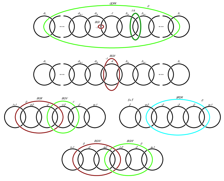
Figure 13. Chain link surgery description of the lens space duals to $S^{1}\times S^{2}$ doubly primitive knots.

3.1. Continued fractions

First we establish a few basic results about continued fractions. These appear throughout the literature in various forms, but it is useful to set notation and collect them here.

Given the continued fraction $[a_{1},\dots,a_{k}]^{-}$, define the numerators and denominators of the “forward” convergents as follows:

$$\begin{array}[]{lll}P_{-1}=0&P_{0}=1&P_{i}=a_{i}P_{i-1}-P_{i-2}\\ Q_{-1}=-1&Q_{0}=0&Q_{i}=a_{i}Q_{i-1}-Q_{i-2}\end{array}$$

Claim 3.1.

For $i=1,\dots,k$, $\frac{P_{i}}{Q_{i}}=[a_{1},\dots,a_{i}]^{-}$ and $P_{i-1}Q_{i}-P_{i}Q_{i-1}=1$.

Proof.

These are immediate when $i=1$, so assume they are true for continued fractions of length up to $i$. Writing

$$[a_{1},\dots,a_{i-1},a_{i},a_{i+1}]^{-}=[a_{1},\dots,a_{i-1},a^{\prime}_{i}]^{-}$$

where $a^{\prime}_{i}=a_{i}-\frac{1}{a_{i+1}}$, the numerator of the forward convergent of the continued fraction on the right hand side is

$$P^{\prime}_{i}=a^{\prime}_{i}P^{\prime}_{i-1}-P^{\prime}_{i-2}=(a_{i}-\frac{1}{a_{i+1}})P_{i-1}-P_{i-2}=-\frac{1}{a_{i+1}}P_{i-1}+a_{i}P_{i-1}-P_{i-2}=-\frac{1}{a_{i+1}}P_{i-1}+P_{i}.$$

Similarly the denominator is $Q^{\prime}_{i}=-\frac{1}{a_{i+1}}Q_{i-1}+Q_{i}$. Then

$$\frac{P_{i+1}}{Q_{i+1}}=\frac{a_{i+1}P_{i}-P_{i-1}}{a_{i+1}Q_{i}-Q_{i-1}}=\frac{P_{i}-\frac{1}{a_{i+1}}P_{i-1}}{Q_{i}-\frac{1}{a_{i+1}}Q_{i-1}}=\frac{P^{\prime}_{i}}{Q^{\prime}_{i}}=[a_{1},\dots,a_{i+1}]^{-}$$

as desired. Also

$$P_{i-1}Q_{i}-P_{i}Q_{i-1}=P_{i-1}(a_{i}Q_{i-1}-Q_{i-2})-(a_{i}P_{i-1}-P_{i-2})Q_{i-1}\\ =P_{i-2}Q_{i-1}-P_{i-1}Q_{i-2}=\dots=P_{-1}Q_{0}-P_{0}Q_{-1}=1.$$

∎

Given the continued fraction $[a_{k},\dots,a_{1}]^{-}$, define the numerators and denominators of the “backward” convergents as follows:

$$\begin{array}[]{lll}p_{-1}=0&p_{0}=1&p_{i}=a_{i}p_{i-1}-p_{i-2}\\ q_{-1}=-1&q_{0}=0&q_{i}=a_{i-1}q_{i-1}-q_{i-2}\end{array}$$

Claim 3.2.

For $i=1,\dots,k$, $\frac{p_{i}}{q_{i}}=[a_{i},\dots,a_{1}]^{-}$ and $q_{i}=p_{i-1}$.

Proof.

These are immediate when $i=1$, so assume they are true for continued fractions of length up to $i$. First $q_{i+1}=a_{i}q_{i}-q_{i-1}=a_{i}p_{i-1}-p_{i-2}=p_{i}$. Then

$$[a_{i+1},a_{i},\dots,a_{1}]^{-}=a_{i+1}-\frac{1}{[a_{i},\dots,a_{1}]^{-}}=a_{i+1}-\frac{1}{p_{i}/p_{i-1}}=\frac{a_{i+1}p_{i}-p_{i-1}}{p_{i}}=\frac{p_{i+1}}{q_{i+1}}.$$

∎

Lemma 3.3.

$\displaystyle[b_{1},\dots,b_{k},c,-b_{k},\dots,-b_{1}]^{-}=\frac{cP_{k}^{2}}{cP_{k}Q_{k}+1}$

Proof.

Notice that for this continued fraction we have $\frac{P_{i}}{Q_{i}}=[b_{1},\dots,b_{i}]^{-}$ and $\frac{p_{i}}{q_{i}}=[-b_{i},\dots,-b_{1}]^{-}$ for $i=1,\dots,k$. Using the definitions of $P_{i}$ and $p_{i}$ one can show that $p_{i}=(-1)^{i}P_{i}$ for $i=1,\dots,k$. Then we have:

$$[b_{1},\dots,b_{k},c,-b_{k},\dots,-b_{1}]^{-} =[b_{1},\dots,b_{k},c-\frac{1}{[-b_{k},\dots,-b_{1}]^{-}}]^{-}=[b_{1},\dots,b_{k},c-\frac{p_{k-1}}{p_{k}}]^{-}=\frac{(c-\frac{p_{k-1}}{p_{k}})P_{k}-P_{k-1}}{(c-\frac{p_{k-1}}{p_{k}})Q_{k}-Q_{k-1}}$$

$$=\frac{cp_{k}P_{k}-p_{k-1}P_{k}-p_{k}P_{k-1}}{cp_{k}Q_{k}-p_{k-1}Q_{k}-p_{k}Q_{k-1}}=\frac{(-1)^{k}cP_{k}P_{k}-(-1)^{k-1}P_{k-1}P_{k}-(-1)^{k}P_{k}P_{k-1}}{(-1)^{k}cP_{k}Q_{k}-(-1)^{k-1}P_{k-1}Q_{k}-(-1)^{k}P_{k}Q_{k-1}}$$

$$=\frac{(-1)^{k}cP_{k}^{2}}{(-1)^{k}cP_{k}Q_{k}+(-1)^{k}(P_{k-1}Q_{k}-P_{k}Q_{k-1})}=\frac{cP_{k}^{2}}{cP_{k}Q_{k}+1}$$

∎

3.2. Homology classes of the duals to the bg, gofk, and spor knots

We now calculate the homology classes of the knots indicated in Figure 13. To do so, orient and index each linear chain link $L=L_{1}\cup\dots\cup L_{n}$ of $n$ components from right to left as in Figure 14. Denote the exterior of this link by $X(L)=S^{3}-N(L)$. Let $\{\mu_{i},\lambda_{i}\}$ be the standard oriented meridian, longitude pair giving a basis for the homology of the boundary of a regular neighborhood of the $i$th component, $H_{1}(\partial N(L_{i}))$. Then $H_{1}(X(L))=\langle\mu_{1},\dots,\mu_{n}\rangle\cong\mathbb{Z}^{n}$. Take $\lambda_{i}$ so that it is represented by the boundary of a meridional disk in $H_{1}(S^{3}-N(L_{i}))$. Then in $H_{1}(X(L))$ we have $\lambda_{i}=\mu_{i-1}+\mu_{i+1}$ for $i\in\{1,\dots,n\}$ where $\mu_{0}=\mu_{n+1}=0$. Let $L(-a_{1},\dots,-a_{n})$ denote the lens space obtained by this surgery description on the chain link $L$ with $-a_{i}$ surgery on the $i$th component. The surgery induces the relation $\lambda_{i}=a_{i}\mu_{i}$ for each $i$ and hence the relation $0=\mu_{i-1}-a_{i}\mu_{i}+\mu_{i+1}$ in $H_{1}(X(L))$. Thus $H_{1}(L(-a_{1},\dots,-a_{n}))=\langle\mu_{1},\dots,\mu_{n}\quad\colon\quad\mu_{i-1}-a_{i}\mu_{i}+\mu_{i+1},i\in\{1,\dots,n\}\rangle$.

Lemma 3.4.

Let $L(p,q)=L(-a_{1},\dots,-a_{n})$ be the lens space described by surgery on the $n$ component chain link with surgery coefficient $-a_{i}$ on the $i$th component so that $\frac{p}{q}=[a_{1},\dots,a_{n}]^{-}$.

Then $\mu_{i}=P_{i-1}\mu_{1}$ in $H_{1}(L(p,q))$ for each $i=1,\dots,n$. In particular, $p=P_{n}$ and $q^{-1}=P_{n-1}$ so that $q\mu_{n}=\mu_{1}$.

Proof.

Since $\mu_{2}=a_{1}\mu_{1}=P_{1}\mu_{1}$ and $\mu_{i+1}=a_{i}\mu_{i}-\mu_{i-1}$, the result follows from the definition of $P_{i}$ and a simple induction argument. Assuming this statement is true up through $i$,

$$\mu_{i+1}=a_{i}\mu_{i}-\mu_{i-1}=a_{i}P_{i-1}\mu_{1}-P_{i-2}\mu_{1}=(a_{i}P_{i-1}-P_{i-2})\mu_{1}=P_{i}\mu_{1}.$$

The last statement follows since $P_{i-1}=Q_{i}^{-1}$ mod $P_{i}$ by Claim 3.1. ∎

Proof of Theorem 1.9.

Figure 13 shows linear chain link surgery descriptions of Lisca’s lens spaces with additional unknotted components that describe knots in these lens spaces. Orient these knots in Figure 13 counter-clockwise. The homology class of each such knot $K$ may be determined in terms of the meridians of the chain link by counting $\mu_{i}$ for each time $K$ runs under the $i$th component to the left and counting $-\mu_{i}$ for each time $K$ runs under the $i$th component to the right. Applying Lemma 3.4 allows us to write the homology class of $K$ in terms of $\mu_{1}$. For the four families of Theorem 1.3, and using its notation, we obtain the following:

• With $(-a_{1},\dots,-a_{4k+1})=(-b_{1},\dots,-b_{2k},-1,b_{2k},\dots,b_{1})$, $\frac{p}{q}=[b_{1},\dots,b_{2k},1,-b_{2k},\dots,b_{1}]^{-}=\frac{m^{2}}{q}$ where $m=P_{2k}$, $d=Q_{2k}$ and $q=P_{2k}Q_{2k}+1=md+1$. This gives both that $1-q=-dm$ and that $qm=m\mod p$. Furthermore $\mu_{1}=q\mu_{4k+1}$.

  • $[K_{\mbox{\sc bgi}}]=-\mu_{2k+1}=-P_{2k}\mu_{1}=-m\mu_{1}=-qm\mu_{4k+1}=-m\mu_{4k+1}$

  • $[K_{\mbox{\sc gofk}}]=\mu_{1}-\mu_{4k+1}=(1-q)\mu_{1}=-dm\mu_{1}=-dqm\mu_{4k+1}=-dm\mu_{4k+1}$

• With $(-a_{1},\dots,-a_{2k+1})=(-b_{1},-b_{2},\dots,-b_{k},-4,b_{k},\dots,b_{k})$, $\frac{p}{q}=[b_{1},\dots,b_{k},4,-b_{k},\dots,-b_{1}]=\frac{m^{2}}{q}$ where $m=2P_{k}$, $d=2Q_{k}$, and $q=4P_{k}Q_{k}+1=md+1$. This gives that $qm=m\mod p$. Furthermore $\mu_{1}=q\mu_{4k+1}$.

  • $[K_{\mbox{\sc bgii}}]=\mu_{k}-2\mu_{k+1}+\mu_{k+2}=(P_{k-1}-2P_{k}+P_{k+1})\mu_{1}=(P_{k-1}-2P_{k}+(4P_{k}-P_{k-1}))\mu_{1}=2P_{k}\mu_{1}=m\mu_{1}=qm\mu_{4k+1}=m\mu_{4k+1}$

• With $(-a_{1},\dots,-a_{6})=(t+1,-s-2,-2,-t-2,-2,s+1)$, $\frac{p}{q}=[-t-1,s+2,2,t+2,2,-s-1]^{-}=\frac{(4+3t+2s+2st)^{2}}{-(3+2s)^{2}(1+t)}$. Then take $m=4+3t+2s+2st$ so that $p=m^{2}$ and $d=-(3+2s)$ so that $q=d(m-1)$. This gives that $d$ is odd, that $(m-1)=-d(1+t)$ from which $d^{-1}m=(1+t)m\mod p$, and that $qm=-dm\mod p$. Furthermore $\mu_{1}=q\mu_{6}$.

  • $[K_{\mbox{\sc bgiii}}]=\mu_{1}+\mu_{4}=(1+P_{3})\mu_{1}=-(4+3t+2s+2st)\mu_{1}=-m\mu_{1}=-qm\mu_{6}=dm\mu_{6}$ and

  • $[K_{\mbox{\sc bgv}}]=\mu_{3}-\mu_{5}=(P_{2}-P_{4})\mu_{1}=(1+t)(4+3t+2s+2st)\mu_{1}=(1+t)m\mu_{1}=d^{-1}m\mu_{1}=d^{-1}qm\mu_{6}=-m\mu_{6}$

  When $t=1$ we have a third knot. Then $(-a_{1},\dots,-a_{6})=(2,-s-2,-2,-3,-2,s+1)$, $\frac{p}{q}=[-2,s+2,2,3,2,-s-1]^{-}=\frac{(7+4s)^{2}}{-2(3+2s)^{2}}$, and $m=1-2d$.

  • $[K_{\mbox{\sc bgiii}}]=-(7+4s)\mu_{1}=-m\mu_{1}=dm\mu_{6}$,

  • $[K_{\mbox{\sc bgv}}]=2(7+4s)\mu_{1}=2m\mu_{1}=-2dm\mu_{6}=(m-1)m\mu_{6}=-m\mu_{6}$, and

  • $[K_{\mbox{\sc spor}}]=\mu_{2}-\mu_{6}=(P_{1}-P_{5})\mu_{1}=4(7+4s)\mu_{1}=4m\mu_{1}=-2m\mu_{6}$.

• With $(-a_{1},\dots,-a_{6})=(t+1,-2,-s-2,-t-2,-2,s+1)$, $\frac{p}{q}=[-t-1,2,s+2,t+2,2,-s-1]^{-}=\frac{(4+3s+3t+2st)^{2}}{-(3+2s)(3+3s+3t+2st)}$. Then take $m=4+3s+3t+2st$ so that $p=m^{2}$ and $d=-(3+2s)$ so that $q=d(m-1)$. This gives both that $(2m+1)=-d(3+2t)$ from which $d^{-1}m=-(3+2t)m\mod p$ and that $qm=-dm\mod p$. Furthermore $\mu_{1}=q\mu_{6}$.

  • $[K_{\mbox{\sc bgiv}}]=\mu_{1}+\mu_{4}=(1+P_{3})\mu_{1}=-(4+3s+3t+2st)\mu_{1}=-m\mu_{1}=-qm\mu_{6}=dm\mu_{6}$

  • $[K^{\prime}_{\mbox{\sc bgiv}}]=\mu_{3}+\mu_{6}=(P_{2}+P_{5})\mu_{1}=-(3+2t)(4+3s+3t+2st)\mu_{1}=d^{-1}m\mu_{1}=d^{-1}qm\mu_{6}=-m\mu_{6}$.

Let $\mu$ and $\mu^{\prime}$ be the homology classes of the two cores of the Heegaard solid tori of $L(p,q)$ suitably oriented so that $q\mu=\mu^{\prime}$. Then, we have $\mu=\mu_{4k+1}$ for (1) and (2) and $\mu=\mu_{6}$ for (3) and (4) in the calculations above. Since a knot’s orientation does not effect its Dehn surgeries, taking both signs of the homology classes above competes the proof of Theorem 1.9. ∎

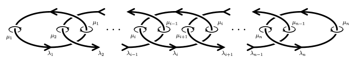
Figure 14.

Lemma 3.5.

The spor knots generically are not Berge-Gabai knots.

In particular, when $t=1$ and $n=s+2\neq-1,0$ the surgery duals to spor, bgiii, bgv are mutually distinct. When $t=1$ and $n=s+2=0$, these knots are all the unknot in $S^{3}$. When $t=1$ and $n=s+2=-1$ the knots spor and bgiii are isotopic but distinct from bgv.

Proof.

Up to mirroring, the lens space obtained by longitudinal surgery on a sporadic knot is $L(p,q)=L((7+4s)^{2},-2(3+2s)^{2})$. Let us reparametrize by $s=n-2$ so that $L(p,q)=L((4n-1)^{2},-2(2n-1)^{2})=L((4n-1)^{2},8n^{2}-1)$. Again, we take $\mu$ and $\mu^{\prime}$ to be the homology classes of the oriented cores of the Heegaard solid tori so that $q\mu=\mu^{\prime}$. Then by Theorem 1.9 the unoriented knot dual to the sporadic knot represents the homology classes $\pm 2(4n-1)\mu$ while the duals to the bgiii and bgv knots in this lens space represent the homology classes $\pm(2n-1)(4n-1)\mu$ and $\pm(4n-1)\mu$. Since $q^{2}\not\equiv\pm 1\pmod{p}$ for $n\neq-1,0$, the group of isotopy classes of diffeomorphisms of our lens space is $\mathbb{Z}/2\mathbb{Z}$, generated by the involution whose quotient is the two bridge link, [13, 28]. This involution acts on $H_{1}(L(p,q))$ as multiplication by $-1$. Therefore when $n\neq-1,0$ (and when $s\neq-3,-2$) the duals to bgiii, bgv, and spor are mutually non-isotopic.

For $n=0$, $L(p,q)=S^{3}$ so that the knot dual to spor, bgiii, and bgv are all the unknot.

For $n=-1$, $L(p,q)=L(25,7)$ the knots dual to spor and bgiii represent the homology classes $\pm 10\mu$. One may directly observe that the corresponding knots are isotopic. The knot dual to bgv represents the homology classes $\pm 5\mu$. The knots in $S^{1}\times S^{2}$ with integral surgeries yielding $L(25,7)$ are those shown to the left and center in Figure 1. ∎

Corollary 3.6.

The three bandings of the two-bridge links in Figure 19 are distinct up to homeomorphism of the two-bridge link.

4. Doubly primitive knots, waves, and simple knots

We now generalize Berge’s results that the duals to doubly primitive knots in $S^{3}$ (under the associated lens space surgery) are simple knots and that $(1,1)$–knots with longitudinal $S^{3}$ surgeries are simple knots. We will adapt Saito’s proofs given in the appendix of [46].

A wave of a genus $2$ Heegaard diagram $(S,\bar{x}=\{x_{1},x_{2}\},\bar{y}=\{y_{1},y_{2}\})$ is an arc $\alpha$ embedded in $S$ so that (up to swapping $x$’s and $y$’s) $\alpha\cap\bar{x}=\partial\alpha\subset x_{i}$ for $i=1$ or $2$, at each endpoint $\alpha$ encounters $x_{i}$ from the same side, and each component of $x_{i}-\alpha$ intersects $\bar{y}$. A regular neighborhood of $\alpha\cup x_{i}$ is a thrice-punctured sphere of which one boundary component is not isotopic to a member of $\bar{x}$. A wave move along $\alpha$ is the replacement of $x_{i}$ by this component.

Let us say two simple closed curves on an orientable surface coherently intersect if they may be oriented so that every intersection occurs with the same sign. (This includes the possibility that the two curves are disjoint.) We then say a Heegaard diagram is coherent if every pair of curves in the diagram coherently intersect.

Say a $3$–manifold $W$ of Heegaard genus at most $2$ is wave-coherent if any genus $2$ Heegaard diagram $(S,\bar{x}=\{x_{1},x_{2}\},\bar{y}=\{y_{1},y_{2}\})$ of $W$ either admits a wave move or is coherent.

Theorem 4.1.

1. If longitudinal surgery on a $(1,1)$–knot in a lens space produces a wave-coherent manifold, then the knot is simple.

2. Given a doubly primitive knot in a wave-coherent manifold of Heegaard genus at most $2$, the surgery dual to the associated lens space surgery is a simple knot.

Proof.

The proof of the first follows exactly the same as that of Saito’s Theorem A.5 (with Lemma A.6) in [46] except that we use Proposition 4.3 below in the stead of his Proposition A.1.

The second item then follows because the surgery dual to a doubly primitive knot is a $(1,1)$–knot. See Theorem A.4 [46] for example. ∎

Corollary 4.2.

A $3$–manifold of genus at most $2$ obtained by longitudinal surgery on a non-trivial $(1,1)$–knot in $S^{3}$ or $S^{1}\times S^{2}$ is not wave-coherent.

Proof.

Theorem 4.1 applies even if the $(1,1)$–knot is in $S^{3}$ or in $S^{1}\times S^{2}$. The trivial knot is the only simple knot in these two manifolds. ∎

Proof of Theorem 1.8.

$S^{1}\times S^{2}$ is wave-coherent by Theorem 1.7 ([35]) so the result follows from Theorem 4.1. ∎

Proposition 4.3 (Cf. Proposition A.1 [46]).

Let $(S;\bar{x}=\{x_{1},x_{2}\},\bar{y}=\{y_{1},y_{2}\})$ be a normalized Heegaard diagram of a $3$–manifold $W$. Assume $z$ is a simple closed curve in $S$ such that $z$ intersects each $x_{1}$ and $y_{1}$ once and is disjoint from both $x_{2}$ and $y_{2}$. If $W$ is wave-coherent, then $x_{2}$ and $y_{2}$ coherently intersect.

Sketch of Proof.

Saito’s proof of the analogous theorem for $W=S^{3}$ applies to any wave-coherent manifold of genus at most $2$ whose genus $2$ Heegaard diagrams enjoy the NEI Property: A Heegaard diagram $(S;\bar{x},\bar{y})$ is said to have the Non-Empty Intersecting (NEI) Property if every $x_{i}\in\bar{x}$ intersects some $y_{j}\in\bar{y}$ and every $y_{j}\in\bar{y}$ intersects some $x_{i}\in\bar{x}$. Any genus $2$ Heegaard diagram for $S^{3}$ (or any homology sphere) enjoys the NEI Property by [37, Lemma 1], and $S^{3}$ is wave-coherent by [29]. The main tool is Ochiai’s structure theorem for Whitehead graphs of genus $2$ Heegaard diagrams with the NEI Property, [37, Theorem 1].

Assume $(S,\bar{x},\bar{y})$ does not enjoy the NEI Property. Then the manifold $W$ contains a non-separating sphere and hence an $S^{1}\times S^{2}$ summand. It follows that $W$ is homeomorphic to $S^{1}\times S^{2}\#L(p,q)$ for some integer $p$. All such manifolds are all wave-coherent by [35, Theorem 1-4].

If $(S,\bar{x},\bar{y})$ is a standard Heegaard diagram for $W\cong S^{1}\times S^{2}\#L(p,q)$, then it is simple and the proposition is satisfied, so further assume the diagram is not standard. Assume $y_{0}\in\{y_{1},y_{2}\}$ does not intersect $x_{1}\cup x_{2}$. Then since the diagram is not standard, $y_{0}$ cannot be parallel to either $x_{1}$ or $x_{2}$. Because $y_{0}$ is non-separating, $y_{0}\cup x_{1}\cup x_{2}$ must be the boundary of thrice-punctured sphere in $S$. Since $z$ intersects $x_{1}$ just once and is disjoint from $x_{2}$, it must also intersect $y_{0}$. Therefore $y_{0}=y_{1}$. Hence the Heegaard diagram with $z$ must appear as in Figure 15 after gluing $x_{i}^{+}$ to $x_{i}^{-}$ for each $i=1,2$ to reform $S$. The thick arcs labeled $a$ and $b$ represent sets of $a$ or $b$ parallel arcs of $y_{2}-(x_{1}\cup x_{2})$. Because $z$ intersects $x_{1}$ once, it dictates how the ends of the rest of the arcs encountering $x_{1}$ must match up. Since these other arcs all together constitute the single curve $y_{2}$, we must have either $b=1$ and $a=0$ or $b=0$ and $a>0$. In either case the conclusion of the proposition holds. ∎

Figure 15.

Question 4.4.

Which $3$–manifolds are wave-coherent? Homma-Ochiai-Takahashi show $S^{3}$ is wave-coherent [29], and Negami-Ochiai show the manifolds $S^{1}\times S^{2}\#L(p,q)$ are wave-coherent [35]. In each of these cases, wave moves reduce genus $2$ Heegaard diagrams into a standard one. On the other hand, note that Osborne shows the lens spaces $L(173,78)$ and $L(85,32)$ admit genus $2$ diagrams with fewer crossings than the standard stabilization of a genus $1$ diagram [38], and hence wave moves alone will not necessarily transform any genus $2$ diagram of these lens spaces into the standard stabilized diagram. Nevertheless these minimal diagrams of Osborne are coherent. Are these lens spaces wave-coherent?

4.1. On the classification of doubly primitive knots in $S^{1}\times S^{2}$

By Theorem 1.8, the surgery dual to a doubly primitive knot in $S^{1}\times S^{2}$ is a simple knot. To prove our families bg, gofk, and spor constitute all doubly primitive knots in $S^{1}\times S^{2}$, it remains to show that no simple knot in Lisca’s lens spaces other than those in the homology classes of Theorem 1.9 admit a surgery to $S^{1}\times S^{2}$.

One approach is to (a) show that the simple knots of the correct homological order in Lisca’s lens spaces have fibered exterior and then (b) determine which of these have planar fibers. Cebanu has confirmed the part (a) employing theorems of Brown [14] and Stallings [47] in the vein of Ozsvath-Szabo’s proof that Berge’s doubly primitive knots are fibered [42]. As of this writing, Cebanu has completed part (b) for the first two types of Lisca’s lens spaces $L(m^{2},md\pm 1)$ where $\gcd(m,d)=1$ or $2$ [15].

One may care to consider alternative approaches of considering either the fundamental group of the result of the homologically correct surgery on the simple knots (see e.g. [48]) or the bandings of the associated tangles.

5. Knots in lens spaces with $S^{1}\times S^{2}$ surgeries from lattice embeddings

Recall from section 1.6 that the expression $\frac{p}{q}=[a_{1},...,a_{n}]^{-}$ with $a_{i}>2$ induces the Kirby diagram of Figure 16 for a negative definite plumbing manifold $P(p,q)$ whose boundary is the lens space $L(p,q)$, and that the $\pi$–rotation $u$ in the diagram describes an involution that expresses $L(p,q)$ as the double cover of $S^{3}$ branched over the two-bridge link $K(p,q)$. See also Figures 4 and 5.

Figure 16. A Kirby diagram of the $4$–manifold $P(p,q)$ with lens space boundary $L(p,q)$.

In his work [33] confirming the slice-ribbon conjecture for two-bridge knots, Lisca observes the following: Assuming $L(p,q)$ smoothly bounds a rational homology ball $W$, then $Z=P(p,q)\cup-W$ is a smooth, closed, negative definite $4$–manifold with $b_{2}(Z)=b_{2}(P(p,q))=n$. Then by Donaldson’s celebrated theorem, the intersection pairing on $H_{2}(Z;\mathbb{Z})$ is isomorphic to $-\operatorname{Id}$. Calling $Q_{p,q}$ the intersection pairing of $P(p,q)$, it follows that the lattice $(\mathbb{Z}^{n},Q_{p,q})$ must embed in the standard negative definite intersection lattice of equal rank; that is, there must exist a monomorphism $\phi\colon\mathbb{Z}^{n}\rightarrow\mathbb{Z}^{n}$ such that $Q_{p,q}(\alpha,\beta)=-\operatorname{Id}(\phi(\alpha),\phi(\beta))$ for all $\alpha,\beta\in\mathbb{Z}^{n}\simeq H_{2}(P(p,q);\mathbb{Z})/\rm{Tors}$.

In determining which lens spaces $L(p,q)$ bound rational homology balls, Lisca determines which of these lattices $(\mathbb{Z}^{n},Q_{p,q})$ admit such an embedding in terms of the coefficients in a continued fraction expansion of $\frac{p}{q}$ by explicitly describing an embedding. Moreover, these embeddings are essentially unique as discussed in Lemma 5.2.

In light of how Greene’s work [25] on embeddings of co-rank 1 lattices with an orthogonal “changemaker” vector yields a classification of the pairs $(L,\kappa)$ of a lens space $L$ and homology class $\kappa\in H_{1}(L)$ of the surgery duals to knots in $S^{3}$, in this section we examine Lisca’s lattice embeddings and determine how they may yield information about the knots dual to these surgeries. (Cf. Remark 1.12.) We observe that these embeddings suggest a method for finding knots in the corresponding lens spaces that admit longitudinal Dehn surgeries to $S^{1}\times S^{2}$. While we do not yet have a formal framework for this construction, the knots we obtain through this method are precisely (the duals to) the Berge-Gabai knots and the gofk knots. Curiously, the duals to the spor knots do not fall out so directly, though knowing they exist we may locate them.

In section 5.1 below we first review Lisca’s classification of which lens spaces bound rational homology balls and make explicit the corresponding lattice embeddings. Then in section 5.2 we describe our procedure for obtaining knots in these lens spaces with longitudinal $S^{1}\times S^{2}$ surgeries and state the results of its application to all of Lisca’s embeddings. We then demonstrate this procedure in section 5.3 with a key example that allows us to compare how the procedure yields bgiii and bgv knots while stops short of yielding the spor knots.

5.1. Lisca’s lens spaces and embeddings of lattices

We shall use the notational shortcut

$$(\dots,2^{[t]},\dots):=(\dots,\overbrace{2,\dots,2}^{t},\dots)$$

Lemma 5.1 (Lisca, [33] Lemmas 7.1, 7.2, 7.3).

If $L(p,q)$ bounds a rational homology ball then $\frac{p}{q}=[a_{1},\dots,a_{n}]^{-}$ or $\frac{p}{q}=[a_{n},\dots,a_{1}]^{-}$ where the string of integers $(-a_{1},\dots,-a_{n})$ is of one of the following types:

$$\begin{array}[]{rll}(1)&(-b_{k},-b_{k-1},\dots,-b_{1},-2,-c_{1},\dots,-c_{l-1},-c_{\ell}),&k,\ell\geq 1,\\ (2)&(-2^{[t]},-3,-2-s,-2-t,-3,-2^{[s]}),&s,t\geq 0,\\ (3)&(-2^{[t]},-3-s,-2,-2-t,-3,-2^{[s]}),&s,t\geq 0,\\ (4)&(-b_{k},-b_{k-1},\dots,-b_{1}-1,-2,-2,-1-c_{1},\dots,-c_{l-1},-c_{\ell}),&k,\ell\geq 1,\\ (5)&(-t-2,-s-2,-3,-2^{[t]},-4,-2^{[s]}),&s,t\geq 0,\\ (6)&(-t-2,-2,-3-s,-2^{[t]},-4,-2^{[s]}),&s,t\geq 0,\\ (7)&(-t-3,-2,-3-s,-3,-2^{[t]},-3,-2^{[s]}),&s,t\geq 0.\end{array}$$

where the $k$–tuple of integers $b_{1},\dots,b_{k}\geq 2$ is arbitrary and the numbers $c_{1},\dots,c_{\ell}\geq 2$ are such that if $\frac{p}{q}=[b_{1},\dots,b_{k}]^{-}$ and $\frac{r}{s}=[c_{1},\dots,c_{\ell}]^{-}$ then $\frac{q}{p}+\frac{s}{r}=1$.

In order to make explicit the embeddings $\phi$ of the lattices defined by the intersection pairings associated to the lens spaces in Lemma 5.1 we need to introduce some notation. Let $E=\{e_{1},\dots,e_{n}\}$ be a basis of the negative diagonal lattice (so that $-\mbox{Id}(e_{i},e_{j})=e_{i}\cdot e_{j}=-\delta_{ij}$) and let $V=\{v_{1},\dots,v_{n}\}$ denote the standard basis of $H_{2}(P(p,q))$ given by the Kirby diagram in Figure 16. We know, from Lisca’s work, that if $\phi(v_{i})=\sum_{j=1}^{n}\lambda_{j}e_{j}$ then $|\lambda_{j}|\leq 1$, and therefore we can summarize $\phi$ as in the following tables, where the signs $+$ and $-$ stand for $\lambda_{j}=+1$ and $\lambda_{j}=-1$ respectively, a blank stands for $\lambda_{j}=0$, and the number in the top left corner refers to the numbering of types in Lemma 5.1. Note that the following holds:

1. $Q_{p,q}(v_{i},v_{i})=\phi(v_{i})\cdot\phi(v_{i})=-a_{i}$,

2. $Q_{p,q}(v_{i},v_{j})=\phi(v_{i})\cdot\phi(v_{j})=1$ if $|i-j|=1$, and

3. $Q_{p,q}(v_{i},v_{j})=\phi(v_{i})\cdot\phi(v_{j})=0$ if $|i-j|>1$.

Whenever the meaning is clear we will drop the $\phi$ from the notation and write $v_{i}=\sum_{j=1}^{n}\lambda_{j}e_{j}$ for $\phi(v_{i})=\sum_{j=1}^{n}\lambda_{j}e_{j}$. First we give embeddings for types (2), (3), (5), (6), and (7) and then we give embeddings for types (1) and (4) as these latter two take on a different character. These are all implicit in [33, Section 7].

$$\begin{array}[]{r|c@{\hspace{0.5mm}}c@{\hspace{0.5mm}}c@{\hspace{0.5mm}}c@{\hspace{0.5mm}}c@{\hspace{0.5mm}}c@{\hspace{0.5mm}}c@{\hspace{0.5mm}}c@{\hspace{0.5mm} }c@{\hspace{0.5mm}}c@{\hspace{0.5mm}}c@{\hspace{0.5mm}}c@{\hspace{0.5mm}}c@{\hspace{0.5mm}}c}(2)&e_{1}\hfil\hskip 1.42262pt&e_{2}\hfil\hskip 1.42262pt&e_{3}\hfil\hskip 1.42262pt&e_{4}\hfil\hskip 1.42262pt&e_{5}\hfil\hskip 1.42262pt&e_{6}\hfil\hskip 1.42262pt&\cdots\hfil\hskip 1.42262pt&e_{t+3}\hfil\hskip 1.42262pt&e_{t+4}\hfil\hskip 1.42262pt&e_{t+5}\hfil\hskip 1.42262pt&e_{t+6}\hfil\hskip 1.42262pt&\cdots\hfil\hskip 1.42262pt&e_{t+s+3}\hfil\hskip 1.42262pt&e_{t+s+4}\\ \hline\cr v_{1}&\hfil\hskip 1.42262pt&\hfil\hskip 1.42262pt&\hfil\hskip 1.42262pt&\hfil\hskip 1.42262pt&\hfil\hskip 1.42262pt&\hfil\hskip 1.42262pt&\hfil\hskip 1.42262pt&-\hfil\hskip 1.42262pt&+\hfil\hskip 1.42262pt&\hfil\hskip 1.42262pt&\hfil\hskip 1.42262pt&\hfil\hskip 1.42262pt&\hfil\hskip 1.42262pt&\\ \vdots&\hfil\hskip 1.42262pt&\hfil\hskip 1.42262pt&\hfil\hskip 1.42262pt&\hfil\hskip 1.42262pt&\hfil\hskip 1.42262pt&\hfil\hskip 1.42262pt&\udots\hfil\hskip 1.42262pt&\hfil\hskip 1.42262pt&\hfil\hskip 1.42262pt&\hfil\hskip 1.42262pt&\hfil\hskip 1.42262pt&\hfil\hskip 1.42262pt&\hfil\hskip 1.42262pt&\\ v_{t-1}&\hfil\hskip 1.42262pt&\hfil\hskip 1.42262pt&\hfil\hskip 1.42262pt&\hfil\hskip 1.42262pt&-\hfil\hskip 1.42262pt&+\hfil\hskip 1.42262pt&\hfil\hskip 1.42262pt&\hfil\hskip 1.42262pt&\hfil\hskip 1.42262pt&\hfil\hskip 1.42262pt&\hfil\hskip 1.42262pt&\hfil\hskip 1.42262pt&\hfil\hskip 1.42262pt&\\ v_{t}&\hfil\hskip 1.42262pt&\hfil\hskip 1.42262pt&-\hfil\hskip 1.42262pt&\hfil\hskip 1.42262pt&+\hfil\hskip 1.42262pt&\hfil\hskip 1.42262pt&\hfil\hskip 1.42262pt&\hfil\hskip 1.42262pt&\hfil\hskip 1.42262pt&\hfil\hskip 1.42262pt&\hfil\hskip 1.42262pt&\hfil\hskip 1.42262pt&\hfil\hskip 1.42262pt&\\ v_{t+1}&\hfil\hskip 1.42262pt&+\hfil\hskip 1.42262pt&+\hfil\hskip 1.42262pt&+\hfil\hskip 1.42262pt&\hfil\hskip 1.42262pt&\hfil\hskip 1.42262pt&\hfil\hskip 1.42262pt&\hfil\hskip 1.42262pt&\hfil\hskip 1.42262pt&\hfil\hskip 1.42262pt&\hfil\hskip 1.42262pt&\hfil\hskip 1.42262pt&\hfil\hskip 1.42262pt&\\ v_{t+2}&+\hfil\hskip 1.42262pt&-\hfil\hskip 1.42262pt&\hfil\hskip 1.42262pt&\hfil\hskip 1.42262pt&\hfil\hskip 1.42262pt&\hfil\hskip 1.42262pt&\hfil\hskip 1.42262pt&\hfil\hskip 1.42262pt&\hfil\hskip 1.42262pt&-\hfil\hskip 1.42262pt&-\hfil\hskip 1.42262pt&\cdots\hfil\hskip 1.42262pt&-\hfil\hskip 1.42262pt&-\\ v_{t+3}&\hfil\hskip 1.42262pt&+\hfil\hskip 1.42262pt&-\hfil\hskip 1.42262pt&\hfil\hskip 1.42262pt&-\hfil\hskip 1.42262pt&-\hfil\hskip 1.42262pt&\cdots\hfil\hskip 1.42262pt&-\hfil\hskip 1.42262pt&-\hfil\hskip 1.42262pt&\hfil\hskip 1.42262pt&\hfil\hskip 1.42262pt&\hfil\hskip 1.42262pt&\hfil\hskip 1.42262pt&\\ v_{t+4}&-\hfil\hskip 1.42262pt&-\hfil\hskip 1.42262pt&\hfil\hskip 1.42262pt&+\hfil\hskip 1.42262pt&\hfil\hskip 1.42262pt&\hfil\hskip 1.42262pt&\hfil\hskip 1.42262pt&\hfil\hskip 1.42262pt&\hfil\hskip 1.42262pt&\hfil\hskip 1.42262pt&\hfil\hskip 1.42262pt&\hfil\hskip 1.42262pt&\hfil\hskip 1.42262pt&\\ v_{t+5}&+\hfil\hskip 1.42262pt&\hfil\hskip 1.42262pt&\hfil\hskip 1.42262pt&\hfil\hskip 1.42262pt&\hfil\hskip 1.42262pt&\hfil\hskip 1.42262pt&\hfil\hskip 1.42262pt&\hfil\hskip 1.42262pt&\hfil\hskip 1.42262pt&+\hfil\hskip 1.42262pt&\hfil\hskip 1.42262pt&\hfil\hskip 1.42262pt&\hfil\hskip 1.42262pt&\\ v_{t+6}&\hfil\hskip 1.42262pt&\hfil\hskip 1.42262pt&\hfil\hskip 1.42262pt&\hfil\hskip 1.42262pt&\hfil\hskip 1.42262pt&\hfil\hskip 1.42262pt&\hfil\hskip 1.42262pt&\hfil\hskip 1.42262pt&\hfil\hskip 1.42262pt&-\hfil\hskip 1.42262pt&+\hfil\hskip 1.42262pt&\hfil\hskip 1.42262pt&\hfil\hskip 1.42262pt&\\ \vdots&\hfil\hskip 1.42262pt&\hfil\hskip 1.42262pt&\hfil\hskip 1.42262pt&\hfil\hskip 1.42262pt&\hfil\hskip 1.42262pt&\hfil\hskip 1.42262pt&\hfil\hskip 1.42262pt&\hfil\hskip 1.42262pt&\hfil\hskip 1.42262pt&\hfil\hskip 1.42262pt&\hfil\hskip 1.42262pt&\ddots\hfil\hskip 1.42262pt&\hfil\hskip 1.42262pt&\\ v_{t+s+4}&\hfil\hskip 1.42262pt&\hfil\hskip 1.42262pt&\hfil\hskip 1.42262pt&\hfil\hskip 1.42262pt&\hfil\hskip 1.42262pt&\hfil\hskip 1.42262pt&\hfil\hskip 1.42262pt&\hfil\hskip 1.42262pt&\hfil\hskip 1.42262pt&\hfil\hskip 1.42262pt&\hfil\hskip 1.42262pt&\hfil\hskip 1.42262pt&-\hfil\hskip 1.42262pt&+\\ \end{array}$$

$$\begin{array}[]{r|c@{\hspace{0.5mm}}c@{\hspace{0.5mm}}c@{\hspace{0.5mm}}c@{\hspace{0.5mm}}c@{\hspace{0.5mm}}c@{\hspace{0.5mm}}c@{\hspace{0.5mm}}c@{\hspace{0.5mm} }c@{\hspace{0.5mm}}c@{\hspace{0.5mm}}c@{\hspace{0.5mm}}c@{\hspace{0.5mm}}c@{\hspace{0.5mm}}c}(3)&e_{1}\hfil\hskip 1.42262pt&e_{2}\hfil\hskip 1.42262pt&e_{3}\hfil\hskip 1.42262pt&e_{4}\hfil\hskip 1.42262pt&e_{5}\hfil\hskip 1.42262pt&e_{6}\hfil\hskip 1.42262pt&\cdots\hfil\hskip 1.42262pt&e_{t+3}\hfil\hskip 1.42262pt&e_{t+4}\hfil\hskip 1.42262pt&e_{t+5}\hfil\hskip 1.42262pt&e_{t+6}\hfil\hskip 1.42262pt&\cdots\hfil\hskip 1.42262pt&e_{t+s+3}\hfil\hskip 1.42262pt&e_{t+s+4}\\ \hline\cr v_{1}&\hfil\hskip 1.42262pt&\hfil\hskip 1.42262pt&\hfil\hskip 1.42262pt&\hfil\hskip 1.42262pt&\hfil\hskip 1.42262pt&\hfil\hskip 1.42262pt&\hfil\hskip 1.42262pt&-\hfil\hskip 1.42262pt&+\hfil\hskip 1.42262pt&\hfil\hskip 1.42262pt&\hfil\hskip 1.42262pt&\hfil\hskip 1.42262pt&\hfil\hskip 1.42262pt&\\ \vdots&\hfil\hskip 1.42262pt&\hfil\hskip 1.42262pt&\hfil\hskip 1.42262pt&\hfil\hskip 1.42262pt&\hfil\hskip 1.42262pt&\hfil\hskip 1.42262pt&\udots\hfil\hskip 1.42262pt&\hfil\hskip 1.42262pt&\hfil\hskip 1.42262pt&\hfil\hskip 1.42262pt&\hfil\hskip 1.42262pt&\hfil\hskip 1.42262pt&\hfil\hskip 1.42262pt&\\ v_{t-1}&\hfil\hskip 1.42262pt&\hfil\hskip 1.42262pt&\hfil\hskip 1.42262pt&\hfil\hskip 1.42262pt&-\hfil\hskip 1.42262pt&+\hfil\hskip 1.42262pt&\hfil\hskip 1.42262pt&\hfil\hskip 1.42262pt&\hfil\hskip 1.42262pt&\hfil\hskip 1.42262pt&\hfil\hskip 1.42262pt&\hfil\hskip 1.42262pt&\hfil\hskip 1.42262pt&\\ v_{t}&\hfil\hskip 1.42262pt&\hfil\hskip 1.42262pt&-\hfil\hskip 1.42262pt&\hfil\hskip 1.42262pt&+\hfil\hskip 1.42262pt&\hfil\hskip 1.42262pt&\hfil\hskip 1.42262pt&\hfil\hskip 1.42262pt&\hfil\hskip 1.42262pt&\hfil\hskip 1.42262pt&\hfil\hskip 1.42262pt&\hfil\hskip 1.42262pt&\hfil\hskip 1.42262pt&\\ v_{t+1}&\hfil\hskip 1.42262pt&+\hfil\hskip 1.42262pt&+\hfil\hskip 1.42262pt&+\hfil\hskip 1.42262pt&\hfil\hskip 1.42262pt&\hfil\hskip 1.42262pt&\hfil\hskip 1.42262pt&\hfil\hskip 1.42262pt&\hfil\hskip 1.42262pt&+\hfil\hskip 1.42262pt&+\hfil\hskip 1.42262pt&\cdots\hfil\hskip 1.42262pt&+\hfil\hskip 1.42262pt&+\\ v_{t+2}&+\hfil\hskip 1.42262pt&-\hfil\hskip 1.42262pt&\hfil\hskip 1.42262pt&\hfil\hskip 1.42262pt&\hfil\hskip 1.42262pt&\hfil\hskip 1.42262pt&\hfil\hskip 1.42262pt&\hfil\hskip 1.42262pt&\hfil\hskip 1.42262pt&\hfil\hskip 1.42262pt&\hfil\hskip 1.42262pt&\hfil\hskip 1.42262pt&\hfil\hskip 1.42262pt&\\ v_{t+3}&\hfil\hskip 1.42262pt&+\hfil\hskip 1.42262pt&-\hfil\hskip 1.42262pt&\hfil\hskip 1.42262pt&-\hfil\hskip 1.42262pt&-\hfil\hskip 1.42262pt&\cdots\hfil\hskip 1.42262pt&-\hfil\hskip 1.42262pt&-\hfil\hskip 1.42262pt&\hfil\hskip 1.42262pt&\hfil\hskip 1.42262pt&\hfil\hskip 1.42262pt&\hfil\hskip 1.42262pt&\\ v_{t+4}&-\hfil\hskip 1.42262pt&-\hfil\hskip 1.42262pt&\hfil\hskip 1.42262pt&+\hfil\hskip 1.42262pt&\hfil\hskip 1.42262pt&\hfil\hskip 1.42262pt&\hfil\hskip 1.42262pt&\hfil\hskip 1.42262pt&\hfil\hskip 1.42262pt&\hfil\hskip 1.42262pt&\hfil\hskip 1.42262pt&\hfil\hskip 1.42262pt&\hfil\hskip 1.42262pt&\\ v_{t+5}&\hfil\hskip 1.42262pt&\hfil\hskip 1.42262pt&\hfil\hskip 1.42262pt&-\hfil\hskip 1.42262pt&\hfil\hskip 1.42262pt&\hfil\hskip 1.42262pt&\hfil\hskip 1.42262pt&\hfil\hskip 1.42262pt&\hfil\hskip 1.42262pt&+\hfil\hskip 1.42262pt&\hfil\hskip 1.42262pt&\hfil\hskip 1.42262pt&\hfil\hskip 1.42262pt&\\ v_{t+6}&\hfil\hskip 1.42262pt&\hfil\hskip 1.42262pt&\hfil\hskip 1.42262pt&\hfil\hskip 1.42262pt&\hfil\hskip 1.42262pt&\hfil\hskip 1.42262pt&\hfil\hskip 1.42262pt&\hfil\hskip 1.42262pt&\hfil\hskip 1.42262pt&-\hfil\hskip 1.42262pt&+\hfil\hskip 1.42262pt&\hfil\hskip 1.42262pt&\hfil\hskip 1.42262pt&\\ \vdots&\hfil\hskip 1.42262pt&\hfil\hskip 1.42262pt&\hfil\hskip 1.42262pt&\hfil\hskip 1.42262pt&\hfil\hskip 1.42262pt&\hfil\hskip 1.42262pt&\hfil\hskip 1.42262pt&\hfil\hskip 1.42262pt&\hfil\hskip 1.42262pt&\hfil\hskip 1.42262pt&\hfil\hskip 1.42262pt&\ddots\hfil\hskip 1.42262pt&\hfil\hskip 1.42262pt&\\ v_{t+s+4}&\hfil\hskip 1.42262pt&\hfil\hskip 1.42262pt&\hfil\hskip 1.42262pt&\hfil\hskip 1.42262pt&\hfil\hskip 1.42262pt&\hfil\hskip 1.42262pt&\hfil\hskip 1.42262pt&\hfil\hskip 1.42262pt&\hfil\hskip 1.42262pt&\hfil\hskip 1.42262pt&\hfil\hskip 1.42262pt&\hfil\hskip 1.42262pt&-\hfil\hskip 1.42262pt&+\\ \end{array}$$

$$\begin{array}[]{r|c@{\hspace{0.5mm}}c@{\hspace{0.5mm}}c@{\hspace{0.5mm}}c@{\hspace{0.5mm}}c@{\hspace{0.5mm}}c@{\hspace{0.5mm}}c@{\hspace{0.5mm}}c@{\hspace{0.5mm} }c@{\hspace{0.5mm}}c@{\hspace{0.5mm}}c@{\hspace{0.5mm}}c@{\hspace{0.5mm}}c@{\hspace{0.5mm}}c}(5)&e_{1}\hfil\hskip 1.42262pt&e_{2}\hfil\hskip 1.42262pt&e_{3}\hfil\hskip 1.42262pt&e_{4}\hfil\hskip 1.42262pt&e_{5}\hfil\hskip 1.42262pt&e_{6}\hfil\hskip 1.42262pt&\cdots\hfil\hskip 1.42262pt&e_{t+3}\hfil\hskip 1.42262pt&e_{t+4}\hfil\hskip 1.42262pt&e_{t+5}\hfil\hskip 1.42262pt&e_{t+6}\hfil\hskip 1.42262pt&\cdots\hfil\hskip 1.42262pt&e_{t+s+3}\hfil\hskip 1.42262pt&e_{t+s+4}\\ \hline\cr v_{1}&+\hfil\hskip 1.42262pt&-\hfil\hskip 1.42262pt&\hfil\hskip 1.42262pt&\hfil\hskip 1.42262pt&+\hfil\hskip 1.42262pt&\hfil\hskip 1.42262pt&\cdots\hfil\hskip 1.42262pt&+\hfil\hskip 1.42262pt&+\hfil\hskip 1.42262pt&\hfil\hskip 1.42262pt&\hfil\hskip 1.42262pt&\hfil\hskip 1.42262pt&\hfil\hskip 1.42262pt&\\ v_{2}&\hfil\hskip 1.42262pt&+\hfil\hskip 1.42262pt&-\hfil\hskip 1.42262pt&\hfil\hskip 1.42262pt&\hfil\hskip 1.42262pt&\hfil\hskip 1.42262pt&\hfil\hskip 1.42262pt&\hfil\hskip 1.42262pt&\hfil\hskip 1.42262pt&-\hfil\hskip 1.42262pt&-\hfil\hskip 1.42262pt&\cdots\hfil\hskip 1.42262pt&-\hfil\hskip 1.42262pt&-\\ v_{3}&-\hfil\hskip 1.42262pt&-\hfil\hskip 1.42262pt&\hfil\hskip 1.42262pt&+\hfil\hskip 1.42262pt&\hfil\hskip 1.42262pt&\hfil\hskip 1.42262pt&\hfil\hskip 1.42262pt&\hfil\hskip 1.42262pt&\hfil\hskip 1.42262pt&\hfil\hskip 1.42262pt&\hfil\hskip 1.42262pt&\hfil\hskip 1.42262pt&\hfil\hskip 1.42262pt&\\ v_{4}&+\hfil\hskip 1.42262pt&\hfil\hskip 1.42262pt&\hfil\hskip 1.42262pt&\hfil\hskip 1.42262pt&-\hfil\hskip 1.42262pt&\hfil\hskip 1.42262pt&\hfil\hskip 1.42262pt&\hfil\hskip 1.42262pt&\hfil\hskip 1.42262pt&\hfil\hskip 1.42262pt&\hfil\hskip 1.42262pt&\hfil\hskip 1.42262pt&\hfil\hskip 1.42262pt&\\ v_{5}&\hfil\hskip 1.42262pt&\hfil\hskip 1.42262pt&\hfil\hskip 1.42262pt&\hfil\hskip 1.42262pt&+\hfil\hskip 1.42262pt&-\hfil\hskip 1.42262pt&\hfil\hskip 1.42262pt&\hfil\hskip 1.42262pt&\hfil\hskip 1.42262pt&\hfil\hskip 1.42262pt&\hfil\hskip 1.42262pt&\hfil\hskip 1.42262pt&\hfil\hskip 1.42262pt&\\ \vdots&\hfil\hskip 1.42262pt&\hfil\hskip 1.42262pt&\hfil\hskip 1.42262pt&\hfil\hskip 1.42262pt&\hfil\hskip 1.42262pt&\hfil\hskip 1.42262pt&\ddots\hfil\hskip 1.42262pt&\hfil\hskip 1.42262pt&\hfil\hskip 1.42262pt&\hfil\hskip 1.42262pt&\hfil\hskip 1.42262pt&\hfil\hskip 1.42262pt&\hfil\hskip 1.42262pt&\\ v_{t+3}&\hfil\hskip 1.42262pt&\hfil\hskip 1.42262pt&\hfil\hskip 1.42262pt&\hfil\hskip 1.42262pt&\hfil\hskip 1.42262pt&\hfil\hskip 1.42262pt&\hfil\hskip 1.42262pt&+\hfil\hskip 1.42262pt&-\hfil\hskip 1.42262pt&\hfil\hskip 1.42262pt&\hfil\hskip 1.42262pt&\hfil\hskip 1.42262pt&\hfil\hskip 1.42262pt&\\ v_{t+4}&\hfil\hskip 1.42262pt&+\hfil\hskip 1.42262pt&+\hfil\hskip 1.42262pt&+\hfil\hskip 1.42262pt&\hfil\hskip 1.42262pt&\hfil\hskip 1.42262pt&\hfil\hskip 1.42262pt&\hfil\hskip 1.42262pt&+\hfil\hskip 1.42262pt&\hfil\hskip 1.42262pt&\hfil\hskip 1.42262pt&\hfil\hskip 1.42262pt&\hfil\hskip 1.42262pt&\\ v_{t+5}&\hfil\hskip 1.42262pt&\hfil\hskip 1.42262pt&-\hfil\hskip 1.42262pt&\hfil\hskip 1.42262pt&\hfil\hskip 1.42262pt&\hfil\hskip 1.42262pt&\hfil\hskip 1.42262pt&\hfil\hskip 1.42262pt&\hfil\hskip 1.42262pt&+\hfil\hskip 1.42262pt&\hfil\hskip 1.42262pt&\hfil\hskip 1.42262pt&\hfil\hskip 1.42262pt&\\ v_{t+6}&\hfil\hskip 1.42262pt&\hfil\hskip 1.42262pt&\hfil\hskip 1.42262pt&\hfil\hskip 1.42262pt&\hfil\hskip 1.42262pt&\hfil\hskip 1.42262pt&\hfil\hskip 1.42262pt&\hfil\hskip 1.42262pt&\hfil\hskip 1.42262pt&-\hfil\hskip 1.42262pt&+\hfil\hskip 1.42262pt&\hfil\hskip 1.42262pt&\hfil\hskip 1.42262pt&\\ \vdots&\hfil\hskip 1.42262pt&\hfil\hskip 1.42262pt&\hfil\hskip 1.42262pt&\hfil\hskip 1.42262pt&\hfil\hskip 1.42262pt&\hfil\hskip 1.42262pt&\hfil\hskip 1.42262pt&\hfil\hskip 1.42262pt&\hfil\hskip 1.42262pt&\hfil\hskip 1.42262pt&\hfil\hskip 1.42262pt&\ddots\hfil\hskip 1.42262pt&\hfil\hskip 1.42262pt&\\ v_{t+s+4}&\hfil\hskip 1.42262pt&\hfil\hskip 1.42262pt&\hfil\hskip 1.42262pt&\hfil\hskip 1.42262pt&\hfil\hskip 1.42262pt&\hfil\hskip 1.42262pt&\hfil\hskip 1.42262pt&\hfil\hskip 1.42262pt&\hfil\hskip 1.42262pt&\hfil\hskip 1.42262pt&\hfil\hskip 1.42262pt&\hfil\hskip 1.42262pt&-\hfil\hskip 1.42262pt&+\\ \end{array}$$

$$\begin{array}[]{r|c@{\hspace{0.5mm}}c@{\hspace{0.5mm}}c@{\hspace{0.5mm}}c@{\hspace{0.5mm}}c@{\hspace{0.5mm}}c@{\hspace{0.5mm}}c@{\hspace{0.5mm}}c@{\hspace{0.5mm} }c@{\hspace{0.5mm}}c@{\hspace{0.5mm}}c@{\hspace{0.5mm}}c@{\hspace{0.5mm}}c@{\hspace{0.5mm}}c}(6)&e_{1}\hfil\hskip 1.42262pt&e_{2}\hfil\hskip 1.42262pt&e_{3}\hfil\hskip 1.42262pt&e_{4}\hfil\hskip 1.42262pt&e_{5}\hfil\hskip 1.42262pt&e_{6}\hfil\hskip 1.42262pt&\cdots\hfil\hskip 1.42262pt&e_{t+3}\hfil\hskip 1.42262pt&e_{t+4}\hfil\hskip 1.42262pt&e_{t+5}\hfil\hskip 1.42262pt&e_{t+6}\hfil\hskip 1.42262pt&\cdots\hfil\hskip 1.42262pt&e_{t+s+3}\hfil\hskip 1.42262pt&e_{t+s+4}\\ \hline\cr v_{1}&+\hfil\hskip 1.42262pt&-\hfil\hskip 1.42262pt&\hfil\hskip 1.42262pt&\hfil\hskip 1.42262pt&+\hfil\hskip 1.42262pt&\hfil\hskip 1.42262pt&\cdots\hfil\hskip 1.42262pt&+\hfil\hskip 1.42262pt&+\hfil\hskip 1.42262pt&\hfil\hskip 1.42262pt&\hfil\hskip 1.42262pt&\hfil\hskip 1.42262pt&\hfil\hskip 1.42262pt&\\ v_{2}&\hfil\hskip 1.42262pt&+\hfil\hskip 1.42262pt&-\hfil\hskip 1.42262pt&\hfil\hskip 1.42262pt&\hfil\hskip 1.42262pt&\hfil\hskip 1.42262pt&\hfil\hskip 1.42262pt&\hfil\hskip 1.42262pt&\hfil\hskip 1.42262pt&\hfil\hskip 1.42262pt&\hfil\hskip 1.42262pt&\hfil\hskip 1.42262pt&\hfil\hskip 1.42262pt&\\ v_{3}&-\hfil\hskip 1.42262pt&-\hfil\hskip 1.42262pt&\hfil\hskip 1.42262pt&+\hfil\hskip 1.42262pt&\hfil\hskip 1.42262pt&\hfil\hskip 1.42262pt&\hfil\hskip 1.42262pt&\hfil\hskip 1.42262pt&\hfil\hskip 1.42262pt&+\hfil\hskip 1.42262pt&+\hfil\hskip 1.42262pt&\cdots\hfil\hskip 1.42262pt&+\hfil\hskip 1.42262pt&+\\ v_{4}&+\hfil\hskip 1.42262pt&\hfil\hskip 1.42262pt&\hfil\hskip 1.42262pt&\hfil\hskip 1.42262pt&-\hfil\hskip 1.42262pt&\hfil\hskip 1.42262pt&\hfil\hskip 1.42262pt&\hfil\hskip 1.42262pt&\hfil\hskip 1.42262pt&\hfil\hskip 1.42262pt&\hfil\hskip 1.42262pt&\hfil\hskip 1.42262pt&\hfil\hskip 1.42262pt&\\ v_{5}&\hfil\hskip 1.42262pt&\hfil\hskip 1.42262pt&\hfil\hskip 1.42262pt&\hfil\hskip 1.42262pt&+\hfil\hskip 1.42262pt&-\hfil\hskip 1.42262pt&\hfil\hskip 1.42262pt&\hfil\hskip 1.42262pt&\hfil\hskip 1.42262pt&\hfil\hskip 1.42262pt&\hfil\hskip 1.42262pt&\hfil\hskip 1.42262pt&\hfil\hskip 1.42262pt&\\ \vdots&\hfil\hskip 1.42262pt&\hfil\hskip 1.42262pt&\hfil\hskip 1.42262pt&\hfil\hskip 1.42262pt&\hfil\hskip 1.42262pt&\hfil\hskip 1.42262pt&\ddots\hfil\hskip 1.42262pt&\hfil\hskip 1.42262pt&\hfil\hskip 1.42262pt&\hfil\hskip 1.42262pt&\hfil\hskip 1.42262pt&\hfil\hskip 1.42262pt&\hfil\hskip 1.42262pt&\\ v_{t+3}&\hfil\hskip 1.42262pt&\hfil\hskip 1.42262pt&\hfil\hskip 1.42262pt&\hfil\hskip 1.42262pt&\hfil\hskip 1.42262pt&\hfil\hskip 1.42262pt&\hfil\hskip 1.42262pt&+\hfil\hskip 1.42262pt&-\hfil\hskip 1.42262pt&\hfil\hskip 1.42262pt&\hfil\hskip 1.42262pt&\hfil\hskip 1.42262pt&\hfil\hskip 1.42262pt&\\ v_{t+4}&\hfil\hskip 1.42262pt&+\hfil\hskip 1.42262pt&+\hfil\hskip 1.42262pt&+\hfil\hskip 1.42262pt&\hfil\hskip 1.42262pt&\hfil\hskip 1.42262pt&\hfil\hskip 1.42262pt&\hfil\hskip 1.42262pt&+\hfil\hskip 1.42262pt&\hfil\hskip 1.42262pt&\hfil\hskip 1.42262pt&\hfil\hskip 1.42262pt&\hfil\hskip 1.42262pt&\\ v_{t+5}&\hfil\hskip 1.42262pt&\hfil\hskip 1.42262pt&\hfil\hskip 1.42262pt&-\hfil\hskip 1.42262pt&\hfil\hskip 1.42262pt&\hfil\hskip 1.42262pt&\hfil\hskip 1.42262pt&\hfil\hskip 1.42262pt&\hfil\hskip 1.42262pt&+\hfil\hskip 1.42262pt&\hfil\hskip 1.42262pt&\hfil\hskip 1.42262pt&\hfil\hskip 1.42262pt&\\ v_{t+6}&\hfil\hskip 1.42262pt&\hfil\hskip 1.42262pt&\hfil\hskip 1.42262pt&\hfil\hskip 1.42262pt&\hfil\hskip 1.42262pt&\hfil\hskip 1.42262pt&\hfil\hskip 1.42262pt&\hfil\hskip 1.42262pt&\hfil\hskip 1.42262pt&-\hfil\hskip 1.42262pt&+\hfil\hskip 1.42262pt&\hfil\hskip 1.42262pt&\hfil\hskip 1.42262pt&\\ \vdots&\hfil\hskip 1.42262pt&\hfil\hskip 1.42262pt&\hfil\hskip 1.42262pt&\hfil\hskip 1.42262pt&\hfil\hskip 1.42262pt&\hfil\hskip 1.42262pt&\hfil\hskip 1.42262pt&\hfil\hskip 1.42262pt&\hfil\hskip 1.42262pt&\hfil\hskip 1.42262pt&\hfil\hskip 1.42262pt&\ddots\hfil\hskip 1.42262pt&\hfil\hskip 1.42262pt&\\ v_{t+s+4}&\hfil\hskip 1.42262pt&\hfil\hskip 1.42262pt&\hfil\hskip 1.42262pt&\hfil\hskip 1.42262pt&\hfil\hskip 1.42262pt&\hfil\hskip 1.42262pt&\hfil\hskip 1.42262pt&\hfil\hskip 1.42262pt&\hfil\hskip 1.42262pt&\hfil\hskip 1.42262pt&\hfil\hskip 1.42262pt&\hfil\hskip 1.42262pt&-\hfil\hskip 1.42262pt&+\\ \end{array}$$

$$\begin{array}[]{r|c@{\hspace{0.5mm}}c@{\hspace{0.5mm}}c@{\hspace{0.5mm}}c@{\hspace{0.5mm}}c@{\hspace{0.5mm}}c@{\hspace{0.5mm}}c@{\hspace{0.5mm}}c@{\hspace{0.5mm} }c@{\hspace{0.5mm}}c@{\hspace{0.5mm}}c@{\hspace{0.5mm}}c@{\hspace{0.5mm}}c@{\hspace{0.5mm}}c@{\hspace{0.5mm}}c}(7)&e_{1}\hfil\hskip 1.42262pt&e_{2}\hfil\hskip 1.42262pt&e_{3}\hfil\hskip 1.42262pt&e_{4}\hfil\hskip 1.42262pt&e_{5}\hfil\hskip 1.42262pt&e_{6}\hfil\hskip 1.42262pt&e_{7}\hfil\hskip 1.42262pt&\cdots\hfil\hskip 1.42262pt&e_{t+4}\hfil\hskip 1.42262pt&e_{t+5}\hfil\hskip 1.42262pt&e_{t+6}\hfil\hskip 1.42262pt&e_{t+7}\hfil\hskip 1.42262pt&\cdots\hfil\hskip 1.42262pt&e_{t+s+4}\hfil\hskip 1.42262pt&e_{t+s+5}\\ \hline\cr v_{1}&+\hfil\hskip 1.42262pt&+\hfil\hskip 1.42262pt&+\hfil\hskip 1.42262pt&\hfil\hskip 1.42262pt&\hfil\hskip 1.42262pt&+\hfil\hskip 1.42262pt&+\hfil\hskip 1.42262pt&\cdots\hfil\hskip 1.42262pt&+\hfil\hskip 1.42262pt&+\hfil\hskip 1.42262pt&\hfil\hskip 1.42262pt&\hfil\hskip 1.42262pt&\hfil\hskip 1.42262pt&\hfil\hskip 1.42262pt&\\ v_{2}&\hfil\hskip 1.42262pt&\hfil\hskip 1.42262pt&-\hfil\hskip 1.42262pt&+\hfil\hskip 1.42262pt&\hfil\hskip 1.42262pt&\hfil\hskip 1.42262pt&\hfil\hskip 1.42262pt&\hfil\hskip 1.42262pt&\hfil\hskip 1.42262pt&\hfil\hskip 1.42262pt&\hfil\hskip 1.42262pt&\hfil\hskip 1.42262pt&\hfil\hskip 1.42262pt&\hfil\hskip 1.42262pt&\\ v_{3}&\hfil\hskip 1.42262pt&-\hfil\hskip 1.42262pt&+\hfil\hskip 1.42262pt&\hfil\hskip 1.42262pt&+\hfil\hskip 1.42262pt&\hfil\hskip 1.42262pt&\hfil\hskip 1.42262pt&\hfil\hskip 1.42262pt&\hfil\hskip 1.42262pt&\hfil\hskip 1.42262pt&+\hfil\hskip 1.42262pt&+\hfil\hskip 1.42262pt&\cdots\hfil\hskip 1.42262pt&+\hfil\hskip 1.42262pt&+\\ v_{4}&+\hfil\hskip 1.42262pt&\hfil\hskip 1.42262pt&-\hfil\hskip 1.42262pt&-\hfil\hskip 1.42262pt&\hfil\hskip 1.42262pt&\hfil\hskip 1.42262pt&\hfil\hskip 1.42262pt&\hfil\hskip 1.42262pt&\hfil\hskip 1.42262pt&\hfil\hskip 1.42262pt&\hfil\hskip 1.42262pt&\hfil\hskip 1.42262pt&\hfil\hskip 1.42262pt&\hfil\hskip 1.42262pt&\\ v_{5}&-\hfil\hskip 1.42262pt&\hfil\hskip 1.42262pt&\hfil\hskip 1.42262pt&\hfil\hskip 1.42262pt&\hfil\hskip 1.42262pt&+\hfil\hskip 1.42262pt&\hfil\hskip 1.42262pt&\hfil\hskip 1.42262pt&\hfil\hskip 1.42262pt&\hfil\hskip 1.42262pt&\hfil\hskip 1.42262pt&\hfil\hskip 1.42262pt&\hfil\hskip 1.42262pt&\hfil\hskip 1.42262pt&\\ v_{6}&\hfil\hskip 1.42262pt&\hfil\hskip 1.42262pt&\hfil\hskip 1.42262pt&\hfil\hskip 1.42262pt&\hfil\hskip 1.42262pt&-\hfil\hskip 1.42262pt&+\hfil\hskip 1.42262pt&\hfil\hskip 1.42262pt&\hfil\hskip 1.42262pt&\hfil\hskip 1.42262pt&\hfil\hskip 1.42262pt&\hfil\hskip 1.42262pt&\hfil\hskip 1.42262pt&\hfil\hskip 1.42262pt&\\ \vdots&\hfil\hskip 1.42262pt&\hfil\hskip 1.42262pt&\hfil\hskip 1.42262pt&\hfil\hskip 1.42262pt&\hfil\hskip 1.42262pt&\hfil\hskip 1.42262pt&\hfil\hskip 1.42262pt&\ddots\hfil\hskip 1.42262pt&\hfil\hskip 1.42262pt&\hfil\hskip 1.42262pt&\hfil\hskip 1.42262pt&\hfil\hskip 1.42262pt&\hfil\hskip 1.42262pt&\hfil\hskip 1.42262pt&\\ v_{t+4}&\hfil\hskip 1.42262pt&\hfil\hskip 1.42262pt&\hfil\hskip 1.42262pt&\hfil\hskip 1.42262pt&\hfil\hskip 1.42262pt&\hfil\hskip 1.42262pt&\hfil\hskip 1.42262pt&\hfil\hskip 1.42262pt&-\hfil\hskip 1.42262pt&+\hfil\hskip 1.42262pt&\hfil\hskip 1.42262pt&\hfil\hskip 1.42262pt&\hfil\hskip 1.42262pt&\hfil\hskip 1.42262pt&\\ v_{t+5}&\hfil\hskip 1.42262pt&+\hfil\hskip 1.42262pt&\hfil\hskip 1.42262pt&\hfil\hskip 1.42262pt&+\hfil\hskip 1.42262pt&\hfil\hskip 1.42262pt&\hfil\hskip 1.42262pt&\hfil\hskip 1.42262pt&\hfil\hskip 1.42262pt&-\hfil\hskip 1.42262pt&\hfil\hskip 1.42262pt&\hfil\hskip 1.42262pt&\hfil\hskip 1.42262pt&\hfil\hskip 1.42262pt&\\ v_{t+6}&\hfil\hskip 1.42262pt&\hfil\hskip 1.42262pt&\hfil\hskip 1.42262pt&\hfil\hskip 1.42262pt&-\hfil\hskip 1.42262pt&\hfil\hskip 1.42262pt&\hfil\hskip 1.42262pt&\hfil\hskip 1.42262pt&\hfil\hskip 1.42262pt&\hfil\hskip 1.42262pt&+\hfil\hskip 1.42262pt&\hfil\hskip 1.42262pt&\hfil\hskip 1.42262pt&\hfil\hskip 1.42262pt&\\ v_{t+7}&\hfil\hskip 1.42262pt&\hfil\hskip 1.42262pt&\hfil\hskip 1.42262pt&\hfil\hskip 1.42262pt&\hfil\hskip 1.42262pt&\hfil\hskip 1.42262pt&\hfil\hskip 1.42262pt&\hfil\hskip 1.42262pt&\hfil\hskip 1.42262pt&\hfil\hskip 1.42262pt&-\hfil\hskip 1.42262pt&+\hfil\hskip 1.42262pt&\hfil\hskip 1.42262pt&\hfil\hskip 1.42262pt&\\ \vdots&\hfil\hskip 1.42262pt&\hfil\hskip 1.42262pt&\hfil\hskip 1.42262pt&\hfil\hskip 1.42262pt&\hfil\hskip 1.42262pt&\hfil\hskip 1.42262pt&\hfil\hskip 1.42262pt&\hfil\hskip 1.42262pt&\hfil\hskip 1.42262pt&\hfil\hskip 1.42262pt&\hfil\hskip 1.42262pt&\hfil\hskip 1.42262pt&\ddots\hfil\hskip 1.42262pt&\hfil\hskip 1.42262pt&\\ v_{t+s+5}&\hfil\hskip 1.42262pt&\hfil\hskip 1.42262pt&\hfil\hskip 1.42262pt&\hfil\hskip 1.42262pt&\hfil\hskip 1.42262pt&\hfil\hskip 1.42262pt&\hfil\hskip 1.42262pt&\hfil\hskip 1.42262pt&\hfil\hskip 1.42262pt&\hfil\hskip 1.42262pt&\hfil\hskip 1.42262pt&\hfil\hskip 1.42262pt&\hfil\hskip 1.42262pt&-\hfil\hskip 1.42262pt&+\\ \end{array}$$

For the embeddings of types (1) and (4) in Lemma 5.1, consider the following two operations preformed on a string of integers

• $(-a_{1},\dots,-a_{n})\longrightarrow(-2,-a_{1},\dots,-a_{n}-1)$

• $(-a_{1},\dots,-a_{n})\longrightarrow(-a_{1}-1,\dots,-a_{n},-2).$

Type (1) strings are obtained from $(-2,-2,-2)$ by performing a sequence of operations (a) and (b). Type (4) strings are obtained analogously from the string $(-3,-2,-2,-3)$. Embeddings of these two strings are give below.

$$\begin{array}[]{r|c@{\hspace{0.5mm}}c@{\hspace{0.5mm}}c}&e_{1}\hfil\hskip 1.42262pt&e_{2}\hfil\hskip 1.42262pt&e_{3}\\ \hline\cr v_{1}&+\hfil\hskip 1.42262pt&-\hfil\hskip 1.42262pt&\\ v_{2}&\hfil\hskip 1.42262pt&+\hfil\hskip 1.42262pt&-\\ v_{3}&-\hfil\hskip 1.42262pt&-\hfil\hskip 1.42262pt&\\ \end{array}\quad\quad\quad\quad\quad\quad\begin{array}[]{r|c@{\hspace{0.5mm}}c@{\hspace{0.5mm}}c@{\hspace{0.5mm}}c}&e_{1}\hfil\hskip 1.42262pt&e_{2}\hfil\hskip 1.42262pt&e_{3}\hfil\hskip 1.42262pt&e_{4}\\ \hline\cr v_{1}&\hfil\hskip 1.42262pt&+\hfil\hskip 1.42262pt&+\hfil\hskip 1.42262pt&+\\ v_{2}&+\hfil\hskip 1.42262pt&-\hfil\hskip 1.42262pt&\hfil\hskip 1.42262pt&\\ v_{3}&\hfil\hskip 1.42262pt&+\hfil\hskip 1.42262pt&-\hfil\hskip 1.42262pt&\\ v_{4}&-\hfil\hskip 1.42262pt&-\hfil\hskip 1.42262pt&\hfil\hskip 1.42262pt&+\\ \end{array}$$

Notice that in both cases there is an $e_{i}$ that appears only in the extremal vectors: $e_{1}$ in type (1) and $e_{4}$ in type (4). This permits operations (a) and (b) to extend to the associated embeddings of the strings. For example, applying operation (a) to $(-2,-2,-2)$ gives $(-2,-2,-2,-3)$ and the embedding above becomes $v^{\prime}_{1}=-e_{1}+e_{4}$, $v_{2}^{\prime}=v_{1}$, $v_{3}^{\prime}=v_{2}$, and $v^{\prime}_{4}=v_{3}-e_{4}$. In a similar fashion one may explicitly obtain the embedding of any string of type (1) or (4).

Lemma 5.2.

The above embeddings are unique up to reindexing the basis vectors and scaling by a factor of $-1$.

Proof.

This follows from the proof of [33, Theorem 6.4] that states that if a negative plumbing associated to a lens space admits an embedding, then this embedding can be obtained from the embedding of the lattice associated to the string $(-2,-2,-2)$ by a sequence of operations called “expansions”. The embedding of $(-2,-2,-2)$ is unique up to reindexing and scaling, and the expansions share this property. On the other hand, the reader can easily check that whenever there is a $-2$–chain in the plumbing, that is $n\geq 1$ consecutive unknots with framing $-2$ in the diagram in Figure 16, the embedding of this chain is unique up to reindexing and scaling. Indeed, the only combination of basis vectors with square $-2$ are given by $\pm e_{i}\pm e_{j}$; and if another $-2$–framed unknot is linked to this one, then its embedding must be of the form $\mp e_{i}\pm e_{k}$ or $\pm e_{k}\mp e_{j}$. Families $(2),(3),(5),(6)$ and $(7)$ in Lemma 5.1 consist of $-2$–chains and at most $4$ unknots with framings different from $-2$. One can check that once the embedding of the $-2$–chains is fixed, the embedding of the rest of the unknots in the diagram is forced, and therefore the embedding is unique up to reindexing and scaling. It remains true for families $(1)$ and $(4)$ that once the embedding of the $-2$–chains is fixed the rest of the embedding is forced. However, since in these two families the number of unknots with framing different from $-2$ is arbitrary, it is more cumbersome to show it directly than to deduce it from Lisca’s general analysis on the embedding of lattices associated to lens spaces. ∎

5.2. Surgeries from lattice embeddings

Here we give a heuristic for finding knots in Lisca’s lens spaces with $S^{1}\times S^{2}$ surgeries from the lattice embeddings. With the assumption that such a knot should be suitably “simple” in some sense, we restrict attention to $-1$ surgery on unknots in the Kirby diagram (and hence blowdowns) that are equivariant with respect to the involution and have an “uncomplicated” presentation in hopes that blowing down such an unknot will lead to further reductions of the Kirby diagram.

To begin such a sequence of reductions we look for a coefficient $a_{j}$ that equals $2$. The corresponding component of the chain link has framing $-2$. A blowdown along an unknot linking this component once will change its framing to $-1$, prompting a subsequent blowdown. Given the lattice embedding, if $a_{j}=2$, then $Q_{p,q}(v_{j},v_{j})=-2$ and $\phi(v_{j})=\varepsilon_{k}e_{k}+\varepsilon_{\ell}e_{\ell}$ for some choices of $k,\ell$ and signs $\varepsilon_{k},\varepsilon_{\ell}=\pm 1$. Select either of these two basis vectors, say $e_{k}$. The vectors $v_{i}$ that have non-trivial $e_{k}$ component then indicate the components of the chain link that some unknot $K$ should link so that blowing down along $K$ should initiate a chain of blowdowns yielding $S^{1}\times S^{2}$.

Thus for each rank $n$ lattice embedding of Lemma 5.1 we have the following procedure:

1. Let $E_{2}\subset E$ be the set of basis vectors $e$ such that $e$ is a component vector of some vector $v$ of weight $-2$.

2. Let $E^{k}_{2}$ be the subset of $E_{2}$ consisting of keystone vectors. A basis vector $e\in E$ is a keystone for the embedding of $V$ if there is a filtration $E=E^{0}\supset E^{1}\supset\dots\supset E^{n}=\emptyset$ such that $E^{j-1}-E^{j}=\{e^{j}\}$, $e^{1}=e$, and for $2\leq j\leq n$ there exists a vector $v^{j}\in V$ whose embedding projects to $\pm e^{j}$ in the lattice spanned by $E^{j-1}$.

3. Given $e_{i}\in E^{k}_{2}$ let $(v_{j},\epsilon_{j})$ be the set of vectors $v_{j}$ with linking number $\epsilon_{j}=e_{i}\cdot v_{j}\neq 0$.

4. Find an oriented unknot $K$ that links component $j$ of the chain link with linking number $\epsilon_{j}$ and is invariant with respect to the involution $u$.

5. Check that $-1$ surgery on $K$ produces $S^{1}\times S^{2}$.

We say such a $K$ obtained by the above manner is “suggested by the lattice embedding”. Note that if $e\in E_{2}$ is a keystone for the embedding of $V$, then we may view $K$ as giving an embedded vector $\phi(v_{K})=\pm e$.

Lattice Embedding Proof of Theorem 1.3.

We need to show that for each lens space in the theorem there is at least one knot with a longitudinal surgery yielding $S^{1}\times S^{2}$. From Lemma 5.1 we know that the lens spaces we need to consider coincide with the lens spaces obtained by surgery on the black diagrams in Figure 17.

Applying the above described heuristic to the types (1)–(7) we find the red and green knots in Figure 17 finishing the proof. We sketch how the procedure runs for the various types.

For each type (2), (3), (5), (6), (7) the set $E_{2}$ is fixed and $E_{2}^{k}$ is easily determined. Moreover, notice that if a keystone vector appears in a $-2$-chain then all basis vectors appearing in the $-2$-chain are keystone vectors. Each of these keystones yields a different unknot in the fourth step of the above procedure. However, all the unknots thus obtained are related to one another by the handle slides described in Figure 18 and therefore yield the same linking types. The embedding suggests two different linking types yielding $S^{1}\times S^{2}$, in red and green in Figure 17, for types (2) and (3) and only one, in red, for types (5), (6), (7).

For types (1) and (4), the set $E_{2}$ depends on sequences $b_{1},\dots,b_{k}$ and $c_{1},\dots,c_{\ell}$. Recall from the end of section 5.1 that these two types, and hence these two sequences, are generated from the “seed” strings $(-2,-2,-2)$ and $(-3,-2,-2,-3)$ respectively by applications of the two operations (a) and (b). The corresponding lattice embeddings of these seeds and their expansions by the operations (a) and (b) are also indicated. For these embeddings of the seeds, the set $E_{2}^{k}$ is easily determined. Upon expansions by the operations (a) and (b), the set $E_{2}^{k}$ for type (1) is seen to partition according to a central $-2$–chain and a $-2$–chain at either end, while for type (4) $E_{2}^{k}$ remains associated to the central $-2$–chain. For each of these partitions we find a knot suggested by the embedding shown in red or green in Figure 17 types (1) and (4). ∎

Lemma 5.3.

The lens space duals to the bg and gofk knots are the knots suggested by the lattice embeddings.

Proof.

By Lemma 5.2 the lattice embeddings for types (1)–(7) above are essentially unique. The different knots suggested by the embedding are then, as explained in the preceding proof, precisely the red and green curves in Figure 17. In section 6.1 we show that these knots do correspond to the duals to the bg and gofk knots: using Kirby calculus we relate the diagrams in Figure 17 with the knots in Figure 13. ∎

Remark 5.4.

The dotted blue unknot in type (3) of Figure 17 corresponds to the family of spor knots when the parameter $t=1$, as shown in section 6.1. These are not suggested by the embedding as we now demonstrate.

Figure 17. Equivariant surgeries yielding $S^{1}\times S^{2}$

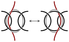
Figure 18. A handle slide of a red curve across a $-2$–framed component of a chain link. The lighter curve indicates the framing.

5.3. Explicit example: type (3), $t=1$, $s=n-2$

In order to understand the duals of the spor knots in the lens spaces we are going to work in full detail the case $L(p_{n},q_{n})=L(16n^{2}-8n+1,16n-2)$ where $\frac{p_{n}}{q_{n}}=\frac{16n^{2}-8n+1}{16n-2}=[2,n+1,2,3,3,2^{[n-2]}]^{-}$. The string of surgery coefficients for the chain link, $(-2,-n-1,-2,-3,-3,-2^{[n-2]})$, shows that all the lens spaces in this example are of type (3) of Lemma 5.1 with $t=1$ and $s=n-2$. From Lisca’s embeddings above we thus obtain the following explicit embedding of the intersection lattice $(\mathbb{Z}^{n+3},Q_{p_{n},q_{n}})$ into the standard negative diagonal lattice of rank $n+3$:

$$\begin{array}[]{r|rrrrrrrrrrrr}&e_{1}&e_{2}&e_{3}&e_{4}&e_{5}&e_{6}&e_{7}&e_{8}&\cdots&e_{n+2}&e_{n+3}\\ \hline\cr v_{1}&&&-&&+&&&&\\ v_{2}&&+&+&+&&+&+&+&\cdots&+&+\\ v_{3}&+&-&&&&&&&\\ v_{4}&&+&-&&-&&&&\\ v_{5}&-&-&&+&&&&&\\ v_{6}&&&&-&&+&&&\\ v_{7}&&&&&&-&+&&\\ v_{8}&&&&&&&-&+&\\ \vdots&&&&&&&&&\ddots\\ v_{n+3}&&&&&&&&&&-&+\\ \end{array}$$

Here we see that $E_{2}=E=\{e_{1},\dots,e_{n+3}\}$ and one may easily check that $E_{2}^{k}=\{e_{1},e_{2},e_{3},e_{5}\}$ and therefore the embedding suggests $4$ possible unknots. However, the reader may check that the unknots obtained from $e_{1}$ and $e_{2}$ are related by a handle slide and so are the two unknots defined by $e_{3}$ and $e_{5}$. A Kirby calculus argument shows that $-1$ surgery on either of these two unknots embedded in $L(p_{n},q_{n})$ yields $S^{1}\times S^{2}$. The unknot related to $e_{1}$ is shown embedded in $L(p_{n},q_{n})$ as the red $1$-framed curve on the top right diagram of Figure19 and the one defined by $e_{3}$ corresponds to the red $-1$-framed curve on the top left diagram of Figure19. Comparing the quotients with Figure 8 we obtain that the unknots suggested by the embedding correspond to the duals of bgiii and bgv.

In order to understand how the family spor in Figure 12 relates to the embedding we turn the surgery on the chain link with coefficients $(-2,-n-1,-2,-3,-3,-2^{[n-2]})$ into a surgery on a $6$ component chain link with coefficients $(-2,-n,2,-1,2,n)$ and lift the spor bands to $L(p_{n},q_{n})$. As a result we obtain that the spor bands lift to the red $0$–framed curve in the bottom diagram of Figure 19. This red curve corresponds to an unknot $K$ with framing $-1$ that satisfies $\phi(v_{K})=\pm e_{n+3}$. This basis vector is not a keystone, since blowing down the unknot $K$ does not prompt a sequence of blow downs yielding a single $0$-framed unknot. In fact, after blowing down $K$ we are led to a surgery diagram with coefficients $\{-2,-2,-2,-3,-2\}$ on a chain link in which the rightmost unknot is linked to the second. The corresponding embedding in the negative standard lattice of rank $5$ is

$$\begin{array}[]{r|c@{\hspace{0.5mm}}c@{\hspace{0.5mm}}c@{\hspace{0.5mm}}c@{\hspace{0.5mm}}c}&e_{1}\hfil\hskip 1.42262pt&e_{2}\hfil\hskip 1.42262pt&e_{3}\hfil\hskip 1.42262pt&e_{4}\hfil\hskip 1.42262pt&e_{5}\\ \hline\cr v^{\prime}_{1}&\hfil\hskip 1.42262pt&\hfil\hskip 1.42262pt&-\hfil\hskip 1.42262pt&\hfil\hskip 1.42262pt&+\\ v^{\prime}_{2}&\hfil\hskip 1.42262pt&+\hfil\hskip 1.42262pt&+\hfil\hskip 1.42262pt&\hfil\hskip 1.42262pt&\\ v^{\prime}_{3}&+\hfil\hskip 1.42262pt&-\hfil\hskip 1.42262pt&\hfil\hskip 1.42262pt&\hfil\hskip 1.42262pt&\\ v^{\prime}_{4}&\hfil\hskip 1.42262pt&+\hfil\hskip 1.42262pt&-\hfil\hskip 1.42262pt&\hfil\hskip 1.42262pt&-\\ v^{\prime}_{5}&-\hfil\hskip 1.42262pt&-\hfil\hskip 1.42262pt&\hfil\hskip 1.42262pt&\hfil\hskip 1.42262pt&\end{array}$$

and the $3$–manifold described by this surgery is $S^{1}\times S^{2}$.

Figure 19. Three copies of a chain link representing $L(16n^{2}-8n+1,16n-2)$ with its two-bridge quotient $K(16n^{2}-8n+1,16n-2)$ below are shown. For each chain link an additional framed red curve is shown representing a knot in a lens space with an $S^{1}\times S^{2}$ surgery; its corresponding banding of the two-bridge link is also shown. The red curves in the top diagrams represent the knots suggested by the embedding for the family of lens spaces $L(16n^{2}-8n+1,16n-2)$ which are the duals of the families bgiii and bgv. In the bottom diagram the red curve represents the dual of the spor band which we obtained by lifting to the lens space the corresponding band in the two bridge link $K(16n^{2}-8n+1,16n-2)$.

Notice that the two first surgeries, the ones corresponding to $e_{1}$ and $e_{3}$, turn the more general family of two bridge links with projection $L(-2^{[k]},-n-1,-2,-2+k,-3,-2^{[n-2]})$ into $S^{1}\times S^{2}$. However, the last surgery described, which corresponds to the spor knots, does not describe such a surgery in this more general family.

6. Kirby calculus and tangle quotients

6.1. Correspondence between Figure 17 and Figure 13

Using Kirby calculus we identify the colored curves in Figure 17 with the corresponding duals to the bg, the gokf and the spor knots shown in Figure 13. We will detail the transition from the first four types in Figure 17 to Figure 13 and sketch the remaining.

Types (1) and (4): Let $L(p,q)$, with $\frac{p}{q}=[a_{1},\dots,a_{n}]^{-}$ and $a_{i}\geq 2$, be the boundary of the $4$–dimensional plumbing manifold $P(p,q)$ given by the Kirby diagram in Figure 16. Blowing up several times one of the final unknots we can turn its framing to $-1$ and after blowing down this $-1$–framed unknot it is not difficult to see that we can continue blowing up and down all the curves in the diagram until we obtain a new Kirby diagram having only positive framings $\geq 2$ and whose boundary is still $L(p,q)$. The $\ell$–tuple of positive framings $(a^{\prime}_{1},\dots,a^{\prime}_{\ell})$ is related to $(-a_{1},\dots,-a_{n})$ by an easy algorithm known as Riemenscheneider point rule [45]. We have that $-L(p,q)=L(p,p-q)$ and a Kirby diagram for $-L(p,q)$ can be obtained from that of $L(p,q)$ by changing the sings of all the framings. It follows that the framings in the negative diagram associated to $L(p,q)$ and the framings in the negative diagram associated to $-L(p,q)$ are related to one another by Riemenschneider point rule. Notice that $\frac{q}{p}+\frac{p-q}{p}=1$, which is the condition defining the framings $(-c_{1},\dots,-c_{\ell})$ from $(-b_{1},\dots,-b_{k})$ for types $(1)$ and $(4)$ in Lemma 5.1. Therefore, a series of blow ups and blow downs changes the framings in types $(1)$ and $(4)$ as follows:

• $(-b_{k},-b_{k-1},\dots,-b_{1},-2,-c_{1},\dots,-c_{l-1},-c_{\ell})\longrightarrow(-b_{k},-b_{k-1},\dots,-b_{1},-1,b_{1},\dots,b_{k-1},b_{k})$

• $(-b_{k},-b_{k-1},\dots,-b_{1}-1,-2,-2,-1-c_{1},\dots,-c_{l-1},-c_{\ell})\longrightarrow(-b_{k},-b_{k-1},\dots,-b_{1}-1,-2,-1,2,b_{1},\dots,b_{k-1},b_{k}).$

In order to obtain the correspondence between Figure 17 and Figure 13 for types (1) and (4), we need to perform the Kirby moves that change the negative plumbing associated to $-L(p,q)$ into the positive one, while taking into account how do the colored curves in Figure 17 change.

The case of type $(4)$ is worked out in full detail in Figure 20. The second diagram is obtained from type $(4)$ in Figure 17 by blowing up the clasp between the $-2$ and the $-c_{1}-1$ framed unknots. Several blow downs and isotopies lead to the fifth diagram in Figure 20. At this point we start performing the above described suite of blowing ups and downs to turn the framings $-c_{i}$ to positive integers $\geq 2$; the first step corresponds to the sixth diagram. The third to last diagram corresponds to the mirror image of the second diagram in Figure 13 with opposite framings. This means that the corresponding lens spaces have the opposite orientation. It follows that type $(4)$ in Figure 17 corresponds to the mirror image of bgii understood as in Figure 13.

Figure 20. Kirby calculus from Type (4), Figure 17 to bgii, Figure 13.

The case of type (1) is very similar to that of type (4). On the one hand, if we consider the lens space diagram, in black, with the red curve, it is clear that when changing the $-c_{i}$ to positive integers the red curve is unaffected. In this way we obtain that the red curve in type $(1)$ corresponds to bgi in Figure 13.

The case of type $(1)$ with the green curve is slightly more delicate. The process of turning the $-c_{i}$ framings to positive integers yields the second diagram in Figure 21. Notice that the framing of the green curve changes to $0$ and that the clasps between each two consecutive unknots are opposite in both sides of the central $-1$. The black diagram cannot be isotoped into a chain of unknots with only right claps without twisting the green curve: in the process the last unknot gains $k$ half twists as illustrated in the last diagram of Figure 21. This diagram shows that the green curve in Family $1$ of Figure 17 corresponds to the gokf curve in Figure 13. Note that in Figure 13 there are $2k$ unknots at each side of the $-1$, this can always be achieved by blowing up once one of the clasps in the last diagram of Figure 21. In Figure 13 the $2k$ half twists are taken into account by means of the $\frac{1}{k}$ framed curve.

Figure 21. Kirby calculus from the green knot in Type (1), Figure 17 to gofk, Figure 13

Type (2): The transformation of type $(2)$ in Figure 17 is detailed in Figure 22. We start changing the two $-2$–chains into single unknots with framings $t$ and $s$. At this point we blow down the two black $-1$–framed curves, changing the framings of the red and green curves, and obtaining the last diagram in Figure 22 which shows that the red and green curve in type $(2)$ Figure 17 correspond to the bgiv in Figure 13 with $t,s\geq 0$.

Figure 22. Kirby calculus from Type (2), Figure 17 to bgiv, Figure 13.

Type (3): The green curve in type $(3)$ in Figure 17 coincides with the bgv diagram in Figure 13. In order to see this we start by changing the two final $-2$–chains in type $(3)$ into two unknots of framings $t+1$ and $s+1$ (just like for type $(2)$). Since the green curve is unaffected by this change in the black diagram it follows that it corresponds to bgv in Figure 13 with $s,t\geq 0$.

The case of the red curve in type $(3)$ is very similar. This time, the last blow down changing the $-2$–chain with $t$ unknots, changes the framing of the red curve to $0$. It is then easy to see that it corresponds to bgiii in Figure 13 with $s,t\geq 0$.

Finally, the case of the blue curve in type $(3)$, with a surgery changing the lens space into $S^{1}\times S^{2}$ when $t=1$, is considered in Figure 23. We start blowing up the clasp between the $-3$–framed unknot and the leftmost unknot in the $-2$–chain and changing the framing of the first unknot from $-2$ to $2$. After several blow downs we arrive to the third diagram of Figure 23. The final blow down of the $-1$–framed unknot changes the framing of the blue curve to $0$ showing that it corresponds to the spor curve in Figure 13 with $s,t\geq 0$.

Figure 23. Kirby calculus from blue knot in Type (3) with $t=1$, Figure 17 to spor, Figure 13

Types (5), (6), (7): Type $(5)$ in Figure 17 is the same as bgiii in Figure 13. The correspondence is established changing the two $-2$–chains into two unknots with framings $t+1$ and $s+1$. This yields a chain of $6$ unknots with framings $(-t-2,-s-2,-2,t+1,-2,s+1)$ which coincides with the framings in the third diagram in Figure 13 after rescaling the parameter $-t-2$ to $t+1$. In the process the red curve’s framing will change to $0$ (cf. type $(2)$) yielding bgiii in Figure 13 with $s\geq 0$ and $t\leq-3$.

By the same argument, type $(6)$ in Figure 17 corresponds to the red bgiv from Figure 13 with $s\geq 0$ and $t\leq-3$ (after rescaling of the parameter $t$ to $-t-3$).

Finally, the transformation of type $(7)$ starts again by changing the $-2$–chains into two unknots with framings $t+1$ and $s+1$. This does not change the red curve. We obtain a chain of six unknots with framings $(-t-3,-2,-3-s,-2,t+1,-1,s+1)$ that rescaled with $t$ replaced by $-s-4$ and $s$ by $t-1$ coincides with the bgv diagram in Figure 13 for $s\leq-4$ and $t\geq 1$.

6.2. From chain link surgery descriptions to tangle descriptions

Figures 24, 25 , 26, 27, and 28 explicitly show how the quotient of these knots with $S^{1}\times S^{2}$ surgeries by the involution $u$ correspond to the bandings of Figures 7, 8, 9, 11, and 12.

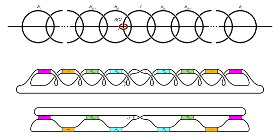
Figure 24.

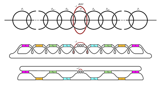
Figure 25.

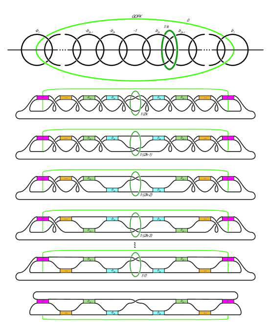
Figure 26.

Figure 27.

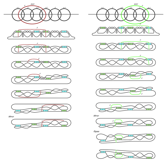
Figure 28.

7. Spherical braids: A proof of Theorem 1.17.

Proof of Theorem 1.17.

Any identification of a solid torus containing a braid with a Heegaard solid torus of $S^{1}\times S^{2}$, produces a spherical braid. Hence the Berge-Gabai knots are spherical braids. (Note that any two such identifications of a solid torus with a Heegaard torus are related by isotopy within $S^{1}\times S^{2}$, mirroring, and inverting the $S^{1}$ direction. Since Berge-Gabai knots in solid tori are invariant under inverting the $S^{1}$ direction, each Berge-Gabai knot in a solid torus gives a unique Berge-Gabai knot in $S^{1}\times S^{2}$ up to mirroring.)

View the genus one fibered knot in $S^{1}\times S^{2}$ as a Hopf band plumbed onto an annulus with trivial monodromy as displayed on the right-hand side of Figure 30. Figure 29 shows the effect of a particular isotopy of the once-punctured torus fiber, realizing the monodromy, upon the core of the annulus (red) and the core of the Hopf band (blue). While most of the isotopy of Figure 29 occurs near the original fiber, the last stage of the isotopy exploits that the ambient manifold is $S^{1}\times S^{2}$ much like the “lightbulb trick” and is highlighted in Figure 30. Using this isotopy or its inverse, one may arrange any curve that lies on the fiber to run along the train track shown on the left-hand side of Figure 31. (See, for example, [43] for the fundamentals of train tracks.) The right-hand side of Figure 31 shows an isotopy of the fiber and the train track so that any curve carried by the train track is a spherical braid. Thus every gofk knot is a spherical braid.

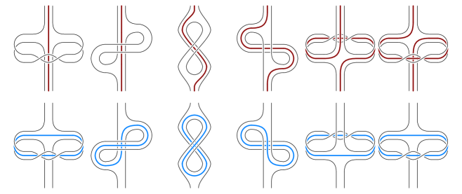
Figure 29.

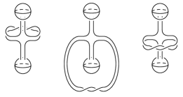
Figure 30.

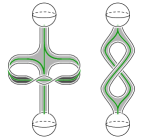
Figure 31. By an isotopy of the once-punctured torus containing this train track into a more “flattened” form, curves carried by the train track are seen to be spherical braids.

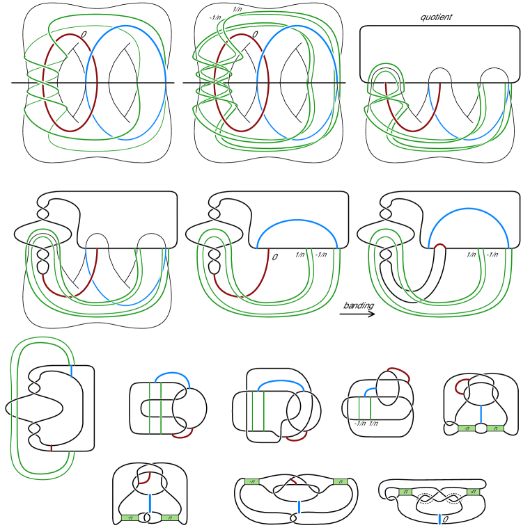
Figure 32.

The bottom right picture in Figure 32 is our tangle version of the sporadic knots in $S^{1}\times S^{2}$ also shown in the second picture of Figure 12. The top left picture of Figure 32 gives a doubly primitive presentation of these sporadic knots, in blue, in terms of Dehn twists along the green curve and $0$–surgery on the red curve as described in the caption. In this picture one may observe that right handed Dehn twists along the green curve keeps the blue curve braided about the red curve. One may also check that after an isotopy, left handed Dehn twists will braid the blue curve about the red too. Hence after $0$–surgery, the resulting blue curve is a spherical braid in $S^{1}\times S^{2}$. ∎

References

- [1] Colin C. Adams, Volumes of hyperbolic -orbifolds with multiple cusps, Indiana Univ. Math. J. 41 (1992), no. 1, 149–172. MR 1160907 (93c:57011)
- [2] James Bailey and Dale Rolfsen, An unexpected surgery construction of a lens space, Pacific J. Math. 71 (1977), no. 2, 295–298. MR 0488061 (58 #7633)
- [3] Kenneth L. Baker, Counting genus one fibered knots in lens spaces, preprint arXiv:math.GT/0510391.
- [4] by same author, Surgery descriptions and volumes of Berge knots. I. Large volume Berge knots, J. Knot Theory Ramifications 17 (2008), no. 9, 1077–1097. MR 2457837 (2009h:57025)
- [5] by same author, Surgery descriptions and volumes of Berge knots. II. Descriptions on the minimally twisted five chain link, J. Knot Theory Ramifications 17 (2008), no. 9, 1099–1120. MR 2457838 (2009h:57026)
- [6] Kenneth L. Baker and Dorothy Buck, The classification of rational subtangle replacements between rational tangles, preprint, To appear in Geom. Topol.
- [7] Kenneth L. Baker and J. Elisenda Grigsby, Grid diagrams and Legendrian lens space links, J. Symplectic Geom. 7 (2009), no. 4, 415–448. MR 2552000 (2011g:57003)
- [8] Kenneth L. Baker, J. Elisenda Grigsby, and Matthew Hedden, Grid diagrams for lens spaces and combinatorial knot Floer homology, Int. Math. Res. Not. IMRN (2008), no. 10, Art. ID rnm024, 39. MR 2429242 (2009h:57012)
- [9] John Berge, Some knots with surgeries yielding lens spaces, Unpublished manuscript.
- [10] by same author, The knots in which have nontrivial Dehn surgeries that yield , Topology Appl. 38 (1991), no. 1, 1–19. MR 1093862 (92d:57005)
- [11] Steven A. Bleiler, Craig D. Hodgson, and Jeffrey R. Weeks, Cosmetic surgery on knots, Proceedings of the Kirbyfest (Berkeley, CA, 1998), Geom. Topol. Monogr., vol. 2, Geom. Topol. Publ., Coventry, 1999, pp. 23–34 (electronic). MR 1734400 (2000j:57034)
- [12] Steven A. Bleiler and Richard A. Litherland, Lens spaces and Dehn surgery, Proc. Amer. Math. Soc. 107 (1989), no. 4, 1127–1131. MR 984783 (90e:57031)
- [13] Francis Bonahon, Difféotopies des espaces lenticulaires, Topology 22 (1983), no. 3, 305–314. MR 710104 (85d:57008)
- [14] Kenneth S. Brown, Trees, valuations, and the Bieri-Neumann-Strebel invariant, Invent. Math. 90 (1987), no. 3, 479–504. MR 914847 (89e:20060)
- [15] Radu Cebanu, Une généralisation de la propriété ”R”, Ph.D. thesis, Université du Québec à Montréal, Novemeber 2012.
- [16] Marc Culler, C. McA. Gordon, J. Luecke, and Peter B. Shalen, Dehn surgery on knots, Ann. of Math. (2) 125 (1987), no. 2, 237–300. MR 881270 (88a:57026)
- [17] Isabel K. Darcy, Kai Ishihara, Ram K. Medikonduri, and Koya Shimokawa, Rational tangle surgery and xer recombination on catenanes, preprint arXiv:1108.0724 [math.GT].
- [18] Ronald Fintushel and Ronald J. Stern, Constructing lens spaces by surgery on knots, Math. Z. 175 (1980), no. 1, 33–51. MR 595630 (82i:57009a)
- [19] David Gabai, Foliations and the topology of -manifolds. II, J. Differential Geom. 26 (1987), no. 3, 461–478. MR 910017 (89a:57014a)
- [20] by same author, Surgery on knots in solid tori, Topology 28 (1989), no. 1, 1–6. MR 991095 (90h:57005)
- [21] by same author, -bridge braids in solid tori, Topology Appl. 37 (1990), no. 3, 221–235. MR 1082933 (92b:57011)
- [22] C. McA. Gordon, Dehn surgery and satellite knots, Trans. Amer. Math. Soc. 275 (1983), no. 2, 687–708. MR 682725 (84d:57003)
- [23] C. McA. Gordon and J. Luecke, Knots are determined by their complements, J. Amer. Math. Soc. 2 (1989), no. 2, 371–415. MR 965210 (90a:57006a)
- [24] by same author, Knots are determined by their complements, J. Amer. Math. Soc. 2 (1989), no. 2, 371–415. MR 965210 (90a:57006a)
- [25] Joshua Evan Greene, The lens space realization problem, preprint arXiv:1010.6257v1 [math.GT], To appear in Ann. of Math.
- [26] Matthew Hedden, Notions of positivity and the Ozsváth-Szabó concordance invariant, J. Knot Theory Ramifications 19 (2010), no. 5, 617–629. MR 2646650 (2011j:57020)
- [27] by same author, On Floer homology and the Berge conjecture on knots admitting lens space surgeries, Trans. Amer. Math. Soc. 363 (2011), no. 2, 949–968. MR 2728591
- [28] Craig Hodgson and J. H. Rubinstein, Involutions and isotopies of lens spaces, Knot theory and manifolds (Vancouver, B.C., 1983), Lecture Notes in Math., vol. 1144, Springer, Berlin, 1985, pp. 60–96. MR 823282 (87h:57028)
- [29] Tatsuo Homma, Mitsuyuki Ochiai, and Moto-o Takahashi, An algorithm for recognizing in -manifolds with Heegaard splittings of genus two, Osaka J. Math. 17 (1980), no. 3, 625–648. MR 591141 (82i:57013)
- [30] Mark Jankins and Walter D. Neumann, Lectures on Seifert manifolds, Brandeis Lecture Notes, vol. 2, Brandeis University, Waltham, MA, 1983. MR 741334 (85j:57015)
- [31] Teruhisa Kadokami and Yuichi Yamada, Lens space surgeries along certain 2-component links related with Park’s rational blow down, and Reidemeister-Turaev torsion, preprint arXiv:1204.4577 [math.GT].
- [32] Ana G. Lecuona, On the slice-ribbon conjecture for Montesinos knots, Trans. Amer. Math. Soc. 364 (2012), no. 1, 233–285. MR 2833583 (2012i:57014)
- [33] Paolo Lisca, Lens spaces, rational balls and the ribbon conjecture, Geom. Topol. 11 (2007), 429–472. MR 2302495 (2008a:57008)
- [34] Louise Moser, Elementary surgery along a torus knot, Pacific J. Math. 38 (1971), 737–745. MR 0383406 (52 #4287)
- [35] Seiya Negami and Kazuo Okita, The splittability and triviality of -bridge links, Trans. Amer. Math. Soc. 289 (1985), no. 1, 253–280. MR 779063 (86h:57008)
- [36] Yi Ni, Knot Floer homology detects fibred knots, Invent. Math. 170 (2007), no. 3, 577–608. MR 2357503 (2008j:57053)
- [37] Mitsuyuki Ochiai, Heegaard diagrams and Whitehead graphs, Math. Sem. Notes Kobe Univ. 7 (1979), no. 3, 573–591. MR 567245 (81e:57003)
- [38] R. P. Osborne, Heegaard diagrams of lens spaces, Proc. Amer. Math. Soc. 84 (1982), no. 3, 412–414. MR 640243 (83c:57001)
- [39] Peter Ozsváth and Zoltán Szabó, Absolutely graded Floer homologies and intersection forms for four-manifolds with boundary, Adv. Math. 173 (2003), no. 2, 179–261. MR 1957829 (2003m:57066)
- [40] by same author, Holomorphic disks and three-manifold invariants: properties and applications, Ann. of Math. (2) 159 (2004), no. 3, 1159–1245. MR 2113020 (2006b:57017)
- [41] by same author, Holomorphic disks and topological invariants for closed three-manifolds, Ann. of Math. (2) 159 (2004), no. 3, 1027–1158. MR 2113019 (2006b:57016)
- [42] by same author, On knot Floer homology and lens space surgeries, Topology 44 (2005), no. 6, 1281–1300. MR 2168576 (2006f:57034)
- [43] R. C. Penner and J. L. Harer, Combinatorics of train tracks, Annals of Mathematics Studies, vol. 125, Princeton University Press, Princeton, NJ, 1992. MR 1144770 (94b:57018)
- [44] Jacob Rasmussen, Lens space surgeries and l-space homology spheres, preprint arXiv:0710.2531v1 [math.GT].
- [45] Oswald Riemenschneider, Deformationen von Quotientensingularitäten (nach zyklischen Gruppen), Math. Ann. 209 (1974), 211–248. MR 0367276 (51 #3518)
- [46] Toshio Saito, The dual knots of doubly primitive knots, Osaka J. Math. 45 (2008), no. 2, 403–421. MR 2441947 (2009e:57014)
- [47] John Stallings, On fibering certain -manifolds, Topology of 3-manifolds and related topics (Proc. The Univ. of Georgia Institute, 1961), Prentice-Hall, Englewood Cliffs, N.J., 1962, pp. 95–100. MR 0158375 (28 #1600)
- [48] Motoo Tange, Lens spaces given from -space homology 3-spheres, Experiment. Math. 18 (2009), no. 3, 285–301. MR 2555699 (2011c:57046)
- [49] William P. Thurston, Three-dimensional geometry and topology. Vol. 1, Princeton Mathematical Series, vol. 35, Princeton University Press, Princeton, NJ, 1997, Edited by Silvio Levy. MR 1435975 (97m:57016)
- [50] Shi Cheng Wang, Cyclic surgery on knots, Proc. Amer. Math. Soc. 107 (1989), no. 4, 1091–1094. MR 984820 (90e:57030)
- [51] Shi Cheng Wang and Qing Zhou, Symmetry of knots and cyclic surgery, Trans. Amer. Math. Soc. 330 (1992), no. 2, 665–676. MR 1031244 (92f:57017)
- [52] Ying Qing Wu, Cyclic surgery and satellite knots, Topology Appl. 36 (1990), no. 3, 205–208. MR 1070700 (91k:57009)
- [53] Yuichi Yamada, Generalized rational blow-down, torus knots and Euclidean algorithm, preprint arXiv:0708.2316 [math.GT].