11institutetext: The Mathematical Neuroscience Laboratory
Collège de France / CIRB and INRIA Bang Laboratory
11, place Marcelin Berthelot, 75005 Paris, France Tel.: +33-144271388
11email: jonathan.touboul@college-de-france.fr

Large deviations, dynamics and phase transitions in large stochastic heterogeneous neural networks

Tanguy Cabana    Jonathan Touboul
(Received: date / Accepted: date)
Abstract

We analyze the macroscopic behavior of multi-populations randomly connected neural networks with interaction delays. Similar to cases occurring in spin glasses, we show that the sequences of empirical measures satisfy a large deviation principle, and converge towards a self-consistent non-Markovian process. The proof differs in that we are working in infinite-dimensional spaces (interaction delays), non-centered interactions and multiple cell types. The limit equation is qualitatively analyzed, and we identify a number of phase transitions in such systems upon changes in delays, connectivity patterns and dispersion, particularly focusing on the emergence of non-equilibrium states involving synchronized oscillations.

Keywords:
Heterogeneous neuronal networks Large deviations Mean-field equations
pacs:
87.19.ll 87.19.lc 87.18.Sn 87.19.lm
journal:


1 Introduction

Brain’s activity results from the interplay of an extraordinary large number of neurons gathering into large-scale populations. This view is supported by anatomical evidences: neurons with the same dynamics and interconnection properties gather into cortical columns (neural populations) with a diameter of about 50μm50𝜇𝑚50\mu m to 1mm1𝑚𝑚1mm, containing of the order of few thousands to one hundred thousand neurons in charge of specific functions mountcastle:97 . This macroscopic signal emerging from the interaction of a large number of cells is recorded by most non-invasive imaging techniques (EEG/MEG/Optical Imaging and Local Field Potentials). These columns have specific functions and spatial locations resulting in the presence of delays in their interactions due to the transport of information through axons and to the typical time the synaptic machinery needs to transmit it. These delays have a clear role in shaping the neuronal activity, as established by different authors (see e.g. coombes-laing:11 ; series-fregnac:02 ). Each neuron involved in this processing has a nonlinear dynamics and is subject to an intense noise.

This picture motivated the development of models of large-scale activity for stochastic neuronal networks amari:72 ; wilson-cowan:73 ; brunel:00 ; bressloff:09 for different models. Some of the approaches are heuristic, and other based on statistical physics methods. Recently, extensions of the theory of mean-field limits to neuronal systems including spatial extension and delays have been developed in a mathematically rigorous framework touboulNeuralfields:11 ; touboul-hermann-faugeras:11 ; touboulNeuralFieldsDynamics:11 . These papers exhibited the limit as the number of neurons goes to infinity, of multi-population (up to a continuum) neuronal networks in the presence of external noise and delays, and showed an essential role of noise in the qualitative dynamics of the macroscopic activity.

However, all these work overlook a prominent aspect of brain networks. Indeed, deeper analysis of the brain’s connectivity evidence a high degree of heterogeneity, in particular in the interconnections parker:03 ; marder-goaillard:06 . These are due to a number of phenomena, among which intervene the precise number of receptors and the extremely slow plasticity mechanisms. All these phenomena induce a static disorder termed static random synaptic heterogeneities. Moreover, thermal noise, channel noise and the intrinsically noisy mechanisms of release and binding of neurotransmitter aldo-faisal:08 result in stochastic variations of the synaptic weights termed stochastic synaptic noise.

Experimental studies of cortical areas aradi-soltesz:02 showed that the degree of heterogeneity in the connections significantly impacts the input-output function, rhythmicity and synchrony. Yet, qualitative effects induced by connection heterogeneities are still poorly understood theoretically. One notable exception is the work of Sompolinsky and collaborators sompolinsky-crisanti-etal:88 . In the thermodynamic limit of a one-population firing-rate neuronal network with synaptic weights modeled as centered independent Gaussian random variables, they evidenced a phase transition between a stationary and a chaotic regime as the disorder is increased. More recently, we showed touboul-hermann:12 that an additional phase transition towards synchronized activity could occur upon increase of the heterogeneity in multi-populations networks.

The topic of the present manuscript is to analyze in a mathematically rigorous manner the effect of heterogeneities and noise in large-scale networks in the presence of delays. One objective of the present manuscript is to understand from a mathematical perspective the mean-field equations used by Sompolinsky and colleagues in sompolinsky-crisanti-etal:88 and to generalize their approach in order to be closer from the biological problem that motivates this study. The paper is organized as follows. In section 2, we will present the mathematical framework and the equations that will be studied throughout the paper, and in particular the inclusion of interaction delays between cells, multiple populations and non-centered synaptic coefficients which were not present of prior models analyzed. From a mathematical perspective, this problem falls in the class of interacting diffusions in a random environment and is reminiscent of the work developed by Ben Arous and Guionnet on the Sherrington-Kirpatrick model ben-arous-guionnet:95 ; guionnet:97 for spin-glass dynamics. Following their approach, we will extend their framework in order to address our biological problem. A heuristic physical argument and a summary of the results is provided in that section, and proofs will be presented in section 3 and appendix A. Similarly to their analysis of spin glass dynamics, we will use large-deviation techniques to characterize the macroscopic limits of these systems in the limit where the number of neurons tends to infinity. There are two main technical distinctions with existing literature. First is the fact that we deal with multi-populations networks, which involves highly nontrivial difficulties, some of which will be further analyzed in a forthcoming study. Second, the fact that the connectivity weights are not centered introduce additional terms that need special care. And third is the presence of delays in the interactions, leading to work in infinite-dimensional spaces.

The limit of the systems being found, we will analyze the solutions of the asymptotic system in section 4. Fortunately, we will show that the solutions of the limit system has Gaussian solutions that are exponentially attractive. These Gaussian solutions are univocally characterized by their mean and covariance functions, and these variables satisfy a closed set of deterministic equations, similar to the ones generally used by physicists from the dynamic mean-field theory sompolinsky-crisanti-etal:88 . The mean satisfies a delayed differential equation coupled to the variance of the solution. These are extremely hard to study analytically. In particular, in contrast with the case of deterministic synaptic weights touboul-hermann-faugeras:11 ; touboulNeuralFieldsDynamics:11 , the variance does not satisfies an ordinary differential equation but can be written as the solution of a fixed point equation. This distinction is fundamentally related to the non-Markovian nature of the asymptotic equation. However, based on the bifurcation analysis of the equation on the mean of the Gaussian solution, an alternative method to more usual analyzes of these mean-field equations, we will be able to characterize the solutions and demonstrate that noise is directly related to the emergence of synchronized oscillations, a highly relevant macroscopic state related to fundamental cortical functions such as memory, attention, sleep and consciousness, and its impairments relate to serious pathologies such as epilepsy or Parkinson’s disease uhlhaas-singer:06 ; buszaki:06 , and that may account for the results of Aradi and colleagues showing that increased heterogeneity was related with epilepsy.

2 Mathematical setting

In this section we introduce the model that we will be investigating in the present manuscript and the main results of the analysis. A heuristic discussion is provided to explain from a physical viewpoint the results that we will establish in section 3.

2.1 The Random Neural Network Model

In all the manuscript, we are working in a complete probability space (Ω,,)Ω(\Omega,\mathcal{F},\mathbbm{P}) endowed with a filtration (t)tsubscriptsubscript𝑡𝑡\big{(}\mathcal{F}_{t}\big{)}_{t} satisfying the usual conditions. We consider a network composed of N𝑁N neurons falling into one of M𝑀M populations. We define by p:{1,,M}:𝑝maps-to1𝑀p:\mathbbm{N}\mapsto\{1,\cdots,M\} the population function associating to a neuron index the population label it belongs to. The state of each neuron i𝑖i in population p(i)=α{1,,M}𝑝𝑖𝛼1𝑀p(i)=\alpha\in\{1,\cdots,M\} is described by its membrane potential xisuperscript𝑥𝑖x^{i}\in\mathbbm{R}, and considered to satisfy a firing-rate equation (similar to the Hopfield network well known to physicists, see amari:72 ; hopfield:82 ; wilson-cowan:72 ):

dxti=(1θαxti+γ=1Mj:p(j)=γJijSαγ(xtταγj))dt+λαdWti𝑑subscriptsuperscript𝑥𝑖𝑡1subscript𝜃𝛼subscriptsuperscript𝑥𝑖𝑡superscriptsubscript𝛾1𝑀subscript:𝑗𝑝𝑗𝛾subscript𝐽𝑖𝑗subscript𝑆𝛼𝛾subscriptsuperscript𝑥𝑗𝑡subscript𝜏𝛼𝛾𝑑𝑡subscript𝜆𝛼𝑑subscriptsuperscript𝑊𝑖𝑡dx^{i}_{t}=\left(-\frac{1}{\theta_{\alpha}}x^{i}_{t}+\sum_{\gamma=1}^{M}\sum_{j:p(j)=\gamma}J_{ij}S_{\alpha\gamma}(x^{j}_{t-\tau_{\alpha\gamma}})\right)\,dt+\lambda_{\alpha}dW^{i}_{t} (1)

where θαsubscript𝜃𝛼\theta_{\alpha} is the characteristic time of neurons of population α𝛼\alpha, Jijsubscript𝐽𝑖𝑗J_{ij} is the synaptic efficiency of the synapse between neuron j𝑗j and neuron i𝑖i, Sαγsubscript𝑆𝛼𝛾S_{\alpha\gamma} the sigmoidal voltage-to-rate function, ταγsubscript𝜏𝛼𝛾\tau_{\alpha\gamma} the propagation delay between neurons of population γ𝛾\gamma and neurons of population α𝛼\alpha, and λαsubscript𝜆𝛼\lambda_{\alpha} the noise intensity. The Brownian motions Wtisubscriptsuperscript𝑊𝑖𝑡W^{i}_{t} account for the noisy input received by all neurons, and the heterogeneity of the connections is integrated in the synaptic weights Jijsubscript𝐽𝑖𝑗J_{ij}. These weights are assumed to be independent Gaussian random variables, with law 𝒩(J¯p(i)p(j)Np(j),σp(i)p(j)Np(j))𝒩subscript¯𝐽𝑝𝑖𝑝𝑗subscript𝑁𝑝𝑗subscript𝜎𝑝𝑖𝑝𝑗subscript𝑁𝑝𝑗\mathcal{N}(\frac{\bar{J}_{p(i)p(j)}}{N_{p(j)}},\frac{\sigma_{p(i)p(j)}}{\sqrt{N_{p(j)}}}), and in the stochastic synaptic noise case, these will be assumed to be stochastic processes, further specified below. Let us emphasize that all the results readily generalize to neurons having a nonlinear intrinsic dynamics:

dxti=(fα(t,xti)+γ=1Mj:p(j)=γJijSαγ(xtταγj))dt+λαdWti𝑑subscriptsuperscript𝑥𝑖𝑡subscript𝑓𝛼𝑡subscriptsuperscript𝑥𝑖𝑡superscriptsubscript𝛾1𝑀subscript:𝑗𝑝𝑗𝛾subscript𝐽𝑖𝑗subscript𝑆𝛼𝛾subscriptsuperscript𝑥𝑗𝑡subscript𝜏𝛼𝛾𝑑𝑡subscript𝜆𝛼𝑑subscriptsuperscript𝑊𝑖𝑡dx^{i}_{t}=\left(f_{\alpha}(t,x^{i}_{t})+\sum_{\gamma=1}^{M}\sum_{j:p(j)=\gamma}J_{ij}S_{\alpha\gamma}(x^{j}_{t-\tau_{\alpha\gamma}})\right)\,dt+\lambda_{\alpha}dW^{i}_{t}

under the condition that the functions fαsubscript𝑓𝛼f_{\alpha} for α{1,,M}𝛼1𝑀\alpha\in\{1,\cdots,M\} satisfy two standard regularity conditions:

  1. 1.

    The functions fαsubscript𝑓𝛼f_{\alpha} are uniformly locally Lipschitz-continuous in their second variable.

  2. 2.

    They satisfy a uniform monotone growth condition: for any t𝑡t\in\mathbbm{R}, xfα(t,x)C(1+x2)𝑥subscript𝑓𝛼𝑡𝑥𝐶1superscript𝑥2xf_{\alpha}(t,x)\leq C(1+x^{2}).

These refinements allow considering more biologically relevant neuron models. However, generalizations of the interaction that would depend on both the pre- and post-synaptic neurons (consisting in replacing the function Sαγ(xtταγj)subscript𝑆𝛼𝛾subscriptsuperscript𝑥𝑗𝑡subscript𝜏𝛼𝛾S_{\alpha\gamma}(x^{j}_{t-\tau_{\alpha\gamma}}) by a nonlinear function b(xti,xtταγj)𝑏subscriptsuperscript𝑥𝑖𝑡subscriptsuperscript𝑥𝑗𝑡subscript𝜏𝛼𝛾b(x^{i}_{t},x^{j}_{t-\tau_{\alpha\gamma}}) in equation (1)) are harder to achieve and the methodology used in the present manuscript cannot be extended to these more general cases.

Let us define τ=maxαγταγ𝜏subscript𝛼𝛾subscript𝜏𝛼𝛾\tau=\max_{\alpha\gamma}\tau_{\alpha\gamma}, and let (μα)α{1M}subscriptsubscript𝜇𝛼𝛼1𝑀(\mu_{\alpha})_{\alpha\in\{1\cdots M\}} a collection of M𝑀M probability distributions on 𝒞τ=𝒞([τ,0],)subscript𝒞𝜏𝒞𝜏0\mathcal{C}_{\tau}=\mathcal{C}([-\tau,0],\mathbbm{R}) that will be used to characterize the initial condition of neurons in population α𝛼\alpha. The initial condition on the network are considered chaotic, given by:

Law of (xt)t[τ,0]=i=1Nμp(i).Law of subscriptsubscript𝑥𝑡𝑡𝜏0superscriptsubscripttensor-product𝑖1𝑁subscript𝜇𝑝𝑖\text{Law of }(x_{t})_{t\in[-\tau,0]}=\bigotimes_{i=1}^{N}\mu_{p(i)}. (2)

The function (Sαγ)α,γ{1,,M}::subscriptsubscript𝑆𝛼𝛾𝛼𝛾1𝑀maps-to(S_{\alpha\gamma})_{\alpha,\gamma\in\{1,\cdots,M\}}:\mathbbm{R}\mapsto\mathbbm{R} are Lipschitz-continuous sigmoidal functions, i.e. non-decreasing functions tending to 00 at -\infty and to 111 at \infty. This model differs from the work of Ben-Arous and Guionnet in that the voltage is not bounded, there exist multiple populations and the interactions are nonlinear and delayed, which sets the problem in an infinite-dimensional space. The first question that may arise at this point is the well-posedness of the system.

Proposition 1

For each JN×N𝐽superscript𝑁𝑁J\in\mathbbm{R}^{N\times N} and T>0𝑇0T>0, there exists a unique weak solution to the system (1) defined on [τ,T]𝜏𝑇[-\tau,T] with initial condition (2). Moreover, this solution is square integrable.

The proof of this result direct stems of standard theory of delayed stochastic differential equations da-prato:92 ; mao:08 . Indeed, the network equations correspond to delayed stochastic differential equation in dimension N𝑁N. For these equations, it is established that existence, uniqueness and square integrability of the solution hold under the assumption that the drift and diffusion functions are Lipschitz-continuous and enjoy a linear growth property, which clearly hold for our system.

Remark 1

Note that if the initial condition was given by (xti)t[τ,0]=ζisubscriptsubscriptsuperscript𝑥𝑖𝑡𝑡𝜏0superscript𝜁𝑖(x^{i}_{t})_{t\in[-\tau,0]}=\zeta^{i} with ζi=μp(i)superscript𝜁𝑖superscriptsubscript𝜇𝑝𝑖\zeta^{i}\operatorname{\stackrel{{\scriptstyle\mathcal{L}}}{{=}}}\mu_{p(i)}, we can also prove strong existence and uniqueness of solutions.

2.2 Heuristic approach to mean-field equations

The mean-field approach consists in reducing the N𝑁N-dimensional delayed stochastic differential equation (1) to a M𝑀M-dimensional equation on the law of the system in the limit where all Nαsubscript𝑁𝛼N_{\alpha}\to\infty. In (1), one needs to characterize the behavior of γ=1Mj:p(j)=γJijSαγ(xtταγj)superscriptsubscript𝛾1𝑀subscript:𝑗𝑝𝑗𝛾subscript𝐽𝑖𝑗subscript𝑆𝛼𝛾subscriptsuperscript𝑥𝑗𝑡subscript𝜏𝛼𝛾\sum_{\gamma=1}^{M}\sum_{j:p(j)=\gamma}J_{ij}S_{\alpha\gamma}(x^{j}_{t-\tau_{\alpha\gamma}}) in the large Nαsubscript𝑁𝛼N_{\alpha} limit. Following the idea of molecular chaos of Boltzmann (”Stoßzahlansatz”), we may assume that all neurons behave independently and independently of the disorder. This physical ansatz is the basis of our heuristical approach. Assuming that the processes xtταγjsubscriptsuperscript𝑥𝑗𝑡subscript𝜏𝛼𝛾x^{j}_{t-\tau_{\alpha\gamma}} and the coefficients Jijsubscript𝐽𝑖𝑗J_{ij} are independent, the local interaction term γ=1Mj:p(j)=γJijSαγ(xtταγj)superscriptsubscript𝛾1𝑀subscript:𝑗𝑝𝑗𝛾subscript𝐽𝑖𝑗subscript𝑆𝛼𝛾subscriptsuperscript𝑥𝑗𝑡subscript𝜏𝛼𝛾\sum_{\gamma=1}^{M}\sum_{j:p(j)=\gamma}J_{ij}S_{\alpha\gamma}(x^{j}_{t-\tau_{\alpha\gamma}}) is a sum of independent gaussian processes. A functional version of the central limit theorem (under suitable regularity and boundedness conditions) would ensure that

γ=1Mj:p(j)=γJijSαγ(xtταγj)Utα,X¯𝒩(γ=1MJ¯αγ𝔼[Sαγ(X¯tταγγ)],γ=1Mσαγ2𝔼[Sαγ(X¯tταγγ)2])superscriptsubscript𝛾1𝑀subscript:𝑗𝑝𝑗𝛾subscript𝐽𝑖𝑗subscript𝑆𝛼𝛾subscriptsuperscript𝑥𝑗𝑡subscript𝜏𝛼𝛾subscriptsuperscript𝑈𝛼¯𝑋𝑡similar-to𝒩superscriptsubscript𝛾1𝑀subscript¯𝐽𝛼𝛾𝔼delimited-[]subscript𝑆𝛼𝛾subscriptsuperscript¯𝑋𝛾𝑡subscript𝜏𝛼𝛾superscriptsubscript𝛾1𝑀superscriptsubscript𝜎𝛼𝛾2𝔼delimited-[]subscript𝑆𝛼𝛾superscriptsubscriptsuperscript¯𝑋𝛾𝑡subscript𝜏𝛼𝛾2\sum_{\gamma=1}^{M}\sum_{j:p(j)=\gamma}J_{ij}S_{\alpha\gamma}(x^{j}_{t-\tau_{\alpha\gamma}})\to U^{\alpha,\bar{X}}_{t}\sim\mathcal{N}\left(\sum_{\gamma=1}^{M}\bar{J}_{\alpha\gamma}\mathbbm{E}\big{[}S_{\alpha\gamma}(\bar{X}^{\gamma}_{t-\tau_{\alpha\gamma}})\big{]},\sum_{\gamma=1}^{M}\sigma_{\alpha\gamma}^{2}\mathbbm{E}\big{[}S_{\alpha\gamma}(\bar{X}^{\gamma}_{t-\tau_{\alpha\gamma}})^{2}\big{]}\right)

where the Gaussian limits are pairwise independent. In other words, under the molecular chaos hypothesis, averaging effects occur at the level of all neurons, and an effective interaction term in the form of a Gaussian process, will be obtained as an effective collective interaction term:

{dX¯tα=(1θαX¯tα+Utα,X¯)dt+λαdWtαUtα,X¯𝒩(γ=1MJ¯αγ𝔼[Sαγ(X¯tταγγ)],γ=1Mσαγ2𝔼[Sαγ(X¯tταγγ)2])pairwiseindependent.cases𝑑subscriptsuperscript¯𝑋𝛼𝑡1subscript𝜃𝛼subscriptsuperscript¯𝑋𝛼𝑡subscriptsuperscript𝑈𝛼¯𝑋𝑡𝑑𝑡subscript𝜆𝛼𝑑subscriptsuperscript𝑊𝛼𝑡otherwisesimilar-tosubscriptsuperscript𝑈𝛼¯𝑋𝑡𝒩superscriptsubscript𝛾1𝑀subscript¯𝐽𝛼𝛾𝔼delimited-[]subscript𝑆𝛼𝛾subscriptsuperscript¯𝑋𝛾𝑡subscript𝜏𝛼𝛾superscriptsubscript𝛾1𝑀superscriptsubscript𝜎𝛼𝛾2𝔼delimited-[]subscript𝑆𝛼𝛾superscriptsubscriptsuperscript¯𝑋𝛾𝑡subscript𝜏𝛼𝛾2𝑝𝑎𝑖𝑟𝑤𝑖𝑠𝑒𝑖𝑛𝑑𝑒𝑝𝑒𝑛𝑑𝑒𝑛𝑡otherwise\displaystyle\begin{cases}d\bar{X}^{\alpha}_{t}=\left(-\frac{1}{\theta_{\alpha}}\bar{X}^{\alpha}_{t}+U^{\alpha,\bar{X}}_{t}\right)\,dt+\lambda_{\alpha}dW^{\alpha}_{t}\\ U^{\alpha,\bar{X}}_{t}\sim\mathcal{N}\left(\sum_{\gamma=1}^{M}\bar{J}_{\alpha\gamma}\mathbbm{E}\big{[}S_{\alpha\gamma}(\bar{X}^{\gamma}_{t-\tau_{\alpha\gamma}})\big{]},\sum_{\gamma=1}^{M}\sigma_{\alpha\gamma}^{2}\mathbbm{E}\big{[}S_{\alpha\gamma}(\bar{X}^{\gamma}_{t-\tau_{\alpha\gamma}})^{2}\big{]}\right)pairwise\;independent.\end{cases} (3)

This is precisely the same kind of results one obtains in the mean-field theory for spin-glasses. From a mathematical viewpoint, the assumptions of independence of the variables xisuperscript𝑥𝑖x^{i} and of the Jijsubscript𝐽𝑖𝑗J_{ij} cannot be rigorously legitimated.

And unfortunately, as is the case in the theory of spin glasses, rigorous approaches up to now rely on relatively abstract methods using in particular large-deviations theory. This is the approach we will now develop. We shall eventually note that a posteriori validation of the intuition provided by this heuristic argument will be obtained as a side result of our analysis: we will indeed show that a propagation of chaos phenomenon occurs in the limit where all Nαsubscript𝑁𝛼N_{\alpha}\to\infty, i.e. that, provided the initial conditions are independent identically distributed for all neurons in the same population, then finite subsets of neurons behave independently for all times and have the same law given by the mean-field equation (3).

2.3 Summary of the results

Mathematical demonstration of such convergence results for multi-populations networks are still to be developed in general settings, and up to our knowledge no result of this kind for multi-populations networks with different population size exist in the literature. In particular, Sanov’s theorem, hinge of most studies for the convergence of large-scale networks with heterogeneities, is still to be proved for such systems where the elements are one of a few populations and not identically distributed. In order to show rigorous results on the dynamics, we will slightly specify the problem and consider that all populations have identical sizes n𝑛n (hence, N=Mn𝑁𝑀𝑛N=Mn). In that case, the analysis can be reduced to the analysis of one-populations systems but with M𝑀M-dimensional variables, whose α{1M}𝛼1𝑀\alpha\in\{1\cdots M\} component is the voltage of one of the neurons in population α𝛼\alpha.

We now group the N𝑁N variables (xi)i=1Nsubscriptsuperscript𝑥𝑖𝑖1𝑁(x^{i})_{i=1\cdots N} into M𝑀M-dimensional variables Xi=(xiα,α=1M)i=1nsuperscript𝑋𝑖subscriptsuperscript𝑥subscript𝑖𝛼𝛼1𝑀𝑖1𝑛X^{i}=(x^{i_{\alpha}},\alpha=1\cdots M)_{i=1\cdots n} where p(iα)=α𝑝subscript𝑖𝛼𝛼p(i_{\alpha})=\alpha, and such that for any ij𝑖𝑗i\neq j, iαjαsubscript𝑖𝛼subscript𝑗𝛼i_{\alpha}\neq j_{\alpha}. The dynamics of these variables, readily deduced from the original network dynamics, can be written in vector form as:

dXti=(LXti+j=1n𝐉ijS(Xt𝝉j))dt+Σd𝐖ti𝑑subscriptsuperscript𝑋𝑖𝑡𝐿subscriptsuperscript𝑋𝑖𝑡superscriptsubscript𝑗1𝑛direct-productsubscript𝐉𝑖𝑗𝑆subscriptsuperscript𝑋𝑗𝑡𝝉𝑑𝑡Σ𝑑subscriptsuperscript𝐖𝑖𝑡dX^{i}_{t}=\left(L\cdot X^{i}_{t}+\sum_{j=1}^{n}\mathbf{J}_{ij}\odot S(X^{j}_{t-\boldsymbol{\tau}})\right)\,dt+\Sigma\cdot d\mathbf{W}^{i}_{t} (4)

where L𝐿L is the diagonal matrix with coefficient (α,α)𝛼𝛼(\alpha,\alpha) equal to 1/θα1subscript𝜃𝛼-1/\theta_{\alpha}, 𝐉ijsubscript𝐉𝑖𝑗\mathbf{J}_{ij} is the M×M𝑀𝑀M\times M matrix with elements (Jiαjβ)α,β=1Msubscriptsubscript𝐽subscript𝑖𝛼subscript𝑗𝛽𝛼𝛽1𝑀(J_{i_{\alpha}j_{\beta}})_{\alpha,\beta=1\cdots M}, and S(Xt𝝉j)𝑆subscriptsuperscript𝑋𝑗𝑡𝝉S(X^{j}_{t-\boldsymbol{\tau}}) is the M×M𝑀𝑀M\times M matrix with elements (α,γ)𝛼𝛾(\alpha,\gamma) given by Sγα(Xtτγαjα)subscript𝑆𝛾𝛼subscriptsuperscript𝑋subscript𝑗𝛼𝑡subscript𝜏𝛾𝛼S_{\gamma\alpha}(X^{j_{\alpha}}_{t-\tau_{\gamma\alpha}}). The linear operator direct-product\odot acts on M×M𝑀𝑀M\times M matrices by giving the diagonal (as a M𝑀M-dimensional vector) of the classical matrix product of two matrices, so that the component α𝛼\alpha of 𝐉ijS(Xt𝝉j)direct-productsubscript𝐉𝑖𝑗𝑆subscriptsuperscript𝑋𝑗𝑡𝝉\mathbf{J}_{ij}\odot S(X^{j}_{t-\boldsymbol{\tau}}) is precisely equal to γ=1MJiαjγSαγ(xtταγjγ)superscriptsubscript𝛾1𝑀subscript𝐽subscript𝑖𝛼subscript𝑗𝛾subscript𝑆𝛼𝛾subscriptsuperscript𝑥subscript𝑗𝛾𝑡subscript𝜏𝛼𝛾\sum_{\gamma=1}^{M}J_{i_{\alpha}j_{\gamma}}S_{\alpha\gamma}(x^{j_{\gamma}}_{t-\tau_{\alpha\gamma}}). ΣΣ\Sigma is the diagonal matrix with diagonal element λαsubscript𝜆𝛼\lambda_{\alpha} and 𝐖ti=(Wtiα)α=1Msubscriptsuperscript𝐖𝑖𝑡subscriptsubscriptsuperscript𝑊subscript𝑖𝛼𝑡𝛼1𝑀\mathbf{W}^{i}_{t}=(W^{i_{\alpha}}_{t})_{\alpha=1\cdots M}.

We now work with an arbitrary fixed time T>0𝑇0T>0 and denote by n(J)superscript𝑛𝐽\mathbbm{Q}^{n}(J) the unique law solution of the network equations (4) restricted to the σ𝜎\sigma-algebra σ(Xsi,1in,τsT)\sigma(X^{i}_{s},1\leq i\leq n,-\tau\leq s\leq T). n(J)superscript𝑛𝐽\mathbbm{Q}^{n}(J) is a probability measure on 𝒞nsuperscript𝒞𝑛\mathcal{C}^{n} where 𝒞𝒞\mathcal{C} is the space of continuous functions of [τ,T]𝜏𝑇[-\tau,T] with value in Msuperscript𝑀\mathbbm{R}^{M}. When neurons are not coupled (i.e. Jij=0subscript𝐽𝑖𝑗0J_{ij}=0 for all (i,j)𝑖𝑗(i,j)), the law of all variables Xtisubscriptsuperscript𝑋𝑖𝑡X^{i}_{t} are identical, independent, and given by the unique solution P𝑃P of the one-dimensional standard SDE:

{dXt=LXtdt+Σd𝐖t(X0)=μ0cases𝑑subscript𝑋𝑡𝐿subscript𝑋𝑡𝑑𝑡Σ𝑑subscript𝐖𝑡otherwisesubscript𝑋0superscriptsuperscript𝜇0otherwise\begin{cases}dX_{t}=LX_{t}dt+\Sigma d\mathbf{W}_{t}\\ (X_{0})\operatorname{\stackrel{{\scriptstyle\mathcal{L}}}{{=}}}\mu^{0}\end{cases} (5)

The uncoupled system hence has the law of the Ornstein-Uhlenbeck process. P𝑃P is the law of this process restricted to the σ𝜎\sigma-algebra 𝒢T=σ(xs,sT)subscript𝒢𝑇𝜎subscript𝑥𝑠𝑠𝑇\mathcal{G}_{T}=\sigma(x_{s},s\leq T), it is a probability measure on the space 𝒞0subscript𝒞0\mathcal{C}_{0} of continuous functions of [0,T]0𝑇[0,T] in Msuperscript𝑀\mathbbm{R}^{M}. We will denote by Pαsubscript𝑃𝛼P_{\alpha} the law of its component α𝛼\alpha (in our case, P=α=1MPαP=\otimes_{\alpha=1}^{M}P_{\alpha}).

We want to study the behavior of the empirical law on each population:

μ^n=1ni=1nδXisubscript^𝜇𝑛1𝑛superscriptsubscript𝑖1𝑛subscript𝛿superscript𝑋𝑖\hat{\mu}_{n}=\frac{1}{n}\sum_{i=1}^{n}\delta_{X^{i}}

under n(J)superscript𝑛𝐽\mathbbm{Q}^{n}(J) where the coefficients Jijsubscript𝐽𝑖𝑗J_{ij} are independent Gaussian with law given above. By a direct application of Girsanov theorem, n(J)superscript𝑛𝐽\mathbbm{Q}^{n}(J) is absolutely continuous with respect to Pnsuperscript𝑃tensor-productabsent𝑛P^{\otimes n} and we have:

dn(J)dPn=exp(i=1n0T(Σ1j=1n𝐉ijS(Xt𝝉j))d𝐖ti120TΣ1j=1n𝐉ijS(Xt𝝉j)2dt)dsuperscript𝑛𝐽dsuperscript𝑃tensor-productabsent𝑛superscriptsubscript𝑖1𝑛superscriptsubscript0𝑇superscriptsuperscriptΣ1superscriptsubscript𝑗1𝑛direct-productsubscript𝐉𝑖𝑗𝑆superscriptsubscript𝑋𝑡𝝉𝑗𝑑superscriptsubscript𝐖𝑡𝑖12superscriptsubscript0𝑇superscriptdelimited-∥∥superscriptΣ1superscriptsubscript𝑗1𝑛direct-productsubscript𝐉𝑖𝑗𝑆subscriptsuperscript𝑋𝑗𝑡𝝉2𝑑𝑡\frac{\text{d}\mathbbm{Q}^{n}(J)}{\text{d}P^{\otimes n}}=\exp\Bigg{(}\sum_{i=1}^{n}\int_{0}^{T}\Big{(}\Sigma^{-1}\cdot\sum_{j=1}^{n}\mathbf{J}_{ij}\odot S(X_{t-\boldsymbol{\tau}}^{j})\Big{)}^{\prime}d\mathbf{W}_{t}^{i}\\ -\frac{1}{2}\int_{0}^{T}\Big{\|}\Sigma^{-1}\sum_{j=1}^{n}\mathbf{J}_{ij}\odot S(X^{j}_{t-\boldsymbol{\tau}})\Big{\|}^{2}dt\Bigg{)} (6)

where the prime denotes the transposition.

The aim of the present manuscript is to prove the following:

Theorem 2.1

Under Qn=𝔼J(n(J))superscript𝑄𝑛subscript𝔼𝐽superscript𝑛𝐽Q^{n}=\mathbbm{E}_{J}(\mathbbm{Q}^{n}(J)) the law of the N𝑁N-neurons system averaged over all possible configurations (realizations of the synaptic weights (Jij)subscript𝐽𝑖𝑗(J_{ij})), the sequence of empirical measures μ^nsubscript^𝜇𝑛\hat{\mu}_{n} converges towards δQsubscript𝛿𝑄\delta_{Q} as n𝑛n goes to infinity for some probability measure Q𝑄Q.

In detail, we will show that the sequence empirical measures μ^nsubscript^𝜇𝑛\hat{\mu}_{n} satisfies a weak large deviation upper bound property and is tight. Precisely, we will demonstrate that:

Theorem 2.2

There exists a good rate function H𝐻H such that for any compact subset K𝐾K of 1+(𝒞)superscriptsubscript1𝒞\mathcal{M}_{1}^{+}(\mathcal{C}) where 𝒞=𝒞([τ,T],M)𝒞𝒞𝜏𝑇superscript𝑀\mathcal{C}=\mathcal{C}([-\tau,T],\mathbbm{R}^{M}):

lim supn1nlogQn(μ^nK)infKH.subscriptlimit-supremum𝑛1𝑛superscript𝑄𝑛subscript^𝜇𝑛𝐾subscriptinfimum𝐾𝐻\limsup_{n\to\infty}\frac{1}{n}\log Q^{n}(\hat{\mu}_{n}\in K)\leq-\inf_{K}H.

Moreover, we will show a tightness result on that sequence, namely:

Theorem 2.3

For any real number ε>0𝜀0\varepsilon>0, there exists a compact subset Kεsubscript𝐾𝜀K_{\varepsilon} such that for any integer n𝑛n,

Qn(μ^nKε)ε.superscript𝑄𝑛subscript^𝜇𝑛subscript𝐾𝜀𝜀Q^{n}(\hat{\mu}_{n}\notin K_{\varepsilon})\leq\varepsilon.

These two results imply the convergence result provided that we characterize uniquely the minima of H𝐻H, which will be the subject of theorem:

Theorem 2.4

The good rate function H𝐻H is such that:

  1. 1.

    It achieves its minimal value at the probability measure QPmuch-less-than𝑄𝑃Q\ll P satisfying the implicit equation:

    dQdP=[α=1M1λα0TGtα,Qα𝑑Wtα12λα20T(Gtα,Qα)2𝑑t]d𝑄d𝑃delimited-[]superscriptsubscript𝛼1𝑀1subscript𝜆𝛼superscriptsubscript0𝑇superscriptsubscript𝐺𝑡𝛼superscript𝑄𝛼differential-dsubscriptsuperscript𝑊𝛼𝑡12superscriptsubscript𝜆𝛼2superscriptsubscript0𝑇superscriptsuperscriptsubscript𝐺𝑡𝛼superscript𝑄𝛼2differential-d𝑡\frac{\text{d}Q}{\text{d}P}=\mathcal{E}\left[\sum_{\alpha=1}^{M}\frac{1}{\lambda_{\alpha}}\int_{0}^{T}G_{t}^{\alpha,Q^{\alpha}}dW^{\alpha}_{t}-\frac{1}{2\lambda_{\alpha}^{2}}\int_{0}^{T}(G_{t}^{\alpha,Q^{\alpha}})^{2}dt\right]

    where \mathcal{E} denotes the expectation over GQ=(Gα,Qα)α=1Msuperscript𝐺𝑄subscriptsuperscript𝐺𝛼superscript𝑄𝛼𝛼1𝑀G^{Q}=(G^{\alpha,Q^{\alpha}})_{\alpha=1\cdots M} a Gaussian process with mean:

    [Gtα,Qα]=γ=1MJ¯αγSαγ(xtταβ)𝑑Qβ(x)delimited-[]subscriptsuperscript𝐺𝛼superscript𝑄𝛼𝑡superscriptsubscript𝛾1𝑀subscript¯𝐽𝛼𝛾subscript𝑆𝛼𝛾subscript𝑥𝑡subscript𝜏𝛼𝛽differential-dsuperscript𝑄𝛽𝑥\mathcal{E}[G^{\alpha,Q^{\alpha}}_{t}]=\sum_{\gamma=1}^{M}\bar{J}_{\alpha\gamma}\int S_{\alpha\gamma}(x_{t-\tau_{\alpha\beta}})dQ^{\beta}(x)

    and covariance:

    [Gtα,QαGsγ,Qγ]=δαγβ=1Mσαβ2Sαβ(xtταβ)Sαβ(xsταβ)𝑑Qβ(x)delimited-[]subscriptsuperscript𝐺𝛼superscript𝑄𝛼𝑡subscriptsuperscript𝐺𝛾superscript𝑄𝛾𝑠subscript𝛿𝛼𝛾superscriptsubscript𝛽1𝑀superscriptsubscript𝜎𝛼𝛽2subscript𝑆𝛼𝛽subscript𝑥𝑡subscript𝜏𝛼𝛽subscript𝑆𝛼𝛽subscript𝑥𝑠subscript𝜏𝛼𝛽differential-dsuperscript𝑄𝛽𝑥\mathcal{E}[G^{\alpha,Q^{\alpha}}_{t}G^{\gamma,Q^{\gamma}}_{s}]=\delta_{\alpha\gamma}\sum_{\beta=1}^{M}\sigma_{\alpha\beta}^{2}\int S_{\alpha\beta}(x_{t-\tau_{\alpha\beta}})S_{\alpha\beta}(x_{s-\tau_{\alpha\beta}})dQ^{\beta}(x)

    where δαγsubscript𝛿𝛼𝛾\delta_{\alpha\gamma} equals 111 if α=γ𝛼𝛾\alpha=\gamma and 00 otherwise.

  2. 2.

    This provides an implicit self-consistent equation on Q𝑄Q the limit distribution, which has a unique solution.

This theorem will be demonstrated in section 3.2.

Eventually, we will show that the unique solution has Gaussian local equilibria (theorem 3.3), with mean (μα(t))α=1Msubscriptsuperscript𝜇𝛼𝑡𝛼1𝑀(\mu^{\alpha}(t))_{\alpha=1\cdots M} and covariance Cαβ(s,t)superscript𝐶𝛼𝛽𝑠𝑡C^{\alpha\beta}(s,t) satisfying the well-posed system of deterministic equations:

μ˙α(t)=1θαμα(t)+γ=1MJ¯αγfαγ(μγ(tταγ),Cαα(tταγ,tταγ))superscript˙𝜇𝛼𝑡1subscript𝜃𝛼superscript𝜇𝛼𝑡superscriptsubscript𝛾1𝑀subscript¯𝐽𝛼𝛾subscript𝑓𝛼𝛾superscript𝜇𝛾𝑡subscript𝜏𝛼𝛾superscript𝐶𝛼𝛼𝑡subscript𝜏𝛼𝛾𝑡subscript𝜏𝛼𝛾\dot{\mu}^{\alpha}(t)=-\frac{1}{\theta_{\alpha}}\mu^{\alpha}(t)+\sum_{\gamma=1}^{M}\bar{J}_{\alpha\gamma}f_{\alpha\gamma}(\mu^{\gamma}(t-\tau_{\alpha\gamma}),C^{\alpha\alpha}(t-\tau_{\alpha\gamma},t-\tau_{\alpha\gamma})) (7)

where fαγ(μ,v)=Sαγ(x)e(xμ)2/2v2πv𝑑xsubscript𝑓𝛼𝛾𝜇𝑣subscriptsubscript𝑆𝛼𝛾𝑥superscript𝑒superscript𝑥𝜇22𝑣2𝜋𝑣differential-d𝑥f_{\alpha\gamma}(\mu,v)=\int_{\mathbbm{R}}S_{\alpha\gamma}(x)\frac{e^{-(x-\mu)^{2}/2v}}{\sqrt{2\pi v}}dx. The covariance is equal to zero when βα𝛽𝛼\beta\neq\alpha and:

Cα(t,s)=e(t+s)/θα[Cα(0,0)+θαλα22(exp2(ts)/θα1)+γ=1Pσαγ20t0se(u+v)/θαΔμ,Cαγ(uταγ,vταγ)𝑑u𝑑v]superscript𝐶𝛼𝑡𝑠superscript𝑒𝑡𝑠subscript𝜃𝛼delimited-[]superscript𝐶𝛼00subscript𝜃𝛼superscriptsubscript𝜆𝛼222𝑡𝑠subscript𝜃𝛼1superscriptsubscript𝛾1𝑃superscriptsubscript𝜎𝛼𝛾2superscriptsubscript0𝑡superscriptsubscript0𝑠superscript𝑒𝑢𝑣subscript𝜃𝛼superscriptsubscriptΔ𝜇𝐶𝛼𝛾𝑢subscript𝜏𝛼𝛾𝑣subscript𝜏𝛼𝛾differential-d𝑢differential-d𝑣C^{\alpha}(t,s)=e^{-(t+s)/\theta_{\alpha}}\Big{[}C^{\alpha}(0,0)+\frac{\theta_{\alpha}\lambda_{\alpha}^{2}}{2}(\exp{2(t\wedge s)/\theta_{\alpha}}-1)+\sum_{\gamma=1}^{P}\sigma_{\alpha\gamma}^{2}\int_{0}^{t}\int_{0}^{s}e^{(u+v)/\theta_{\alpha}}\Delta_{\mu,C}^{\alpha\gamma}(u-\tau_{\alpha\gamma},v-\tau_{\alpha\gamma})dudv\Big{]} (8)

where Δμ,Cαγ(u,v)=𝔼[Sαγ(Xuγ)Sαγ(Xvγ)]superscriptsubscriptΔ𝜇𝐶𝛼𝛾𝑢𝑣𝔼delimited-[]subscript𝑆𝛼𝛾superscriptsubscript𝑋𝑢𝛾subscript𝑆𝛼𝛾superscriptsubscript𝑋𝑣𝛾\Delta_{\mu,C}^{\alpha\gamma}(u,v)=\mathbb{E}\Big{[}S_{\alpha\gamma}(X_{u}^{\gamma})S_{\alpha\gamma}(X_{v}^{\gamma})\Big{]} is a nonlinear function of μγ(u)superscript𝜇𝛾𝑢\mu^{\gamma}(u), μγ(v)superscript𝜇𝛾𝑣\mu^{\gamma}(v), Cγγ(u,v)superscript𝐶𝛾𝛾𝑢𝑣C^{\gamma\gamma}(u,v), Cγγ(u,u)superscript𝐶𝛾𝛾𝑢𝑢C^{\gamma\gamma}(u,u) and Cγγ(v,v)superscript𝐶𝛾𝛾𝑣𝑣C^{\gamma\gamma}(v,v).

In other words, the solution can be written, in law, as the solution of an implicit equation:

dX¯tα=(1θαX¯tα+Utα,X¯)dt+λαdWtα𝑑subscriptsuperscript¯𝑋𝛼𝑡1subscript𝜃𝛼subscriptsuperscript¯𝑋𝛼𝑡subscriptsuperscript𝑈𝛼¯𝑋𝑡𝑑𝑡subscript𝜆𝛼𝑑subscriptsuperscript𝑊𝛼𝑡d\bar{X}^{\alpha}_{t}=\left(-\frac{1}{\theta_{\alpha}}\bar{X}^{\alpha}_{t}+U^{\alpha,\bar{X}}_{t}\right)\,dt+\lambda_{\alpha}dW^{\alpha}_{t} (9)

where the processes (Wtα)subscriptsuperscript𝑊𝛼𝑡(W^{\alpha}_{t}) are independent Brownian motions and the processes Utα,X¯subscriptsuperscript𝑈𝛼¯𝑋𝑡U^{\alpha,\bar{X}}_{t} are Gaussian processes with law as GQsuperscript𝐺𝑄G^{Q} as described in theorem 2.4. These characterizations will be very handy to analyze the qualitative dynamics and phase transitions of the system.

3 Large Deviations and Mean-Field limits

3.1 Construction of the good rate function

The aim of this section is to identify a good rate function for the system that we will use in Theorem 2.2 to show a large deviation principle. In order to introduce our good rate function, it is convenient to analyze for a moment a time-discretization of the equation (section 3.1.1), which will expedite the analysis of our continuous time problem.

3.1.1 Analysis of the discrete time system

Given an integer k𝑘k, we define Δk={0=t0<t1<<tk<tk+1=T}superscriptΔ𝑘0subscript𝑡0subscript𝑡1subscript𝑡𝑘subscript𝑡𝑘1𝑇\Delta^{k}=\big{\{}0=t_{0}<t_{1}<...<t_{k}<t_{k+1}=T\big{\}} a partition of [0,T]0𝑇[0,T] and consider the following dynamics for the neurons of population α𝛼\alpha:

{dxti=(1θαxti+γ=1Mj:p(j)=γJijSαp(j)(xt(k)ταp(j)j))dt+λαdWtit(k)=sup{tlΔk|tlt}Law of (xtα)t[τ,0]=μαNαcases𝑑subscriptsuperscript𝑥𝑖𝑡1subscript𝜃𝛼subscriptsuperscript𝑥𝑖𝑡superscriptsubscript𝛾1𝑀subscript:𝑗𝑝𝑗𝛾subscript𝐽𝑖𝑗subscript𝑆𝛼𝑝𝑗subscriptsuperscript𝑥𝑗superscript𝑡𝑘subscript𝜏𝛼𝑝𝑗𝑑𝑡subscript𝜆𝛼𝑑subscriptsuperscript𝑊𝑖𝑡otherwisesuperscript𝑡𝑘supremumconditional-setsubscript𝑡𝑙superscriptΔ𝑘subscript𝑡𝑙𝑡otherwiseLaw of subscriptsuperscriptsubscript𝑥𝑡𝛼𝑡𝜏0superscriptsubscript𝜇𝛼tensor-productabsentsubscript𝑁𝛼otherwise\begin{cases}dx^{i}_{t}=\left(-\frac{1}{\theta_{\alpha}}x^{i}_{t}+\sum_{\gamma=1}^{M}\sum_{j:p(j)=\gamma}J_{ij}S_{\alpha p(j)}(x^{j}_{t^{(k)}-\tau_{\alpha p(j)}})\right)\,dt+\lambda_{\alpha}dW^{i}_{t}\\ t^{(k)}=\sup\big{\{}t_{l}\in\Delta^{k}|t_{l}\leq t\big{\}}\\ \text{Law of }(x_{t}^{\alpha})_{t\in[-\tau,0]}=\mu_{\alpha}^{\otimes N_{\alpha}}\end{cases} (10)

As in Proposition 1, this system clearly admits a unique weak solution for any JN×N𝐽superscript𝑁𝑁J\in\mathbbm{R}^{N\times N}. We will denote Nα,n(J)superscriptsubscript𝑁𝛼𝑛𝐽\mathbbm{Q}^{N_{\alpha},n}(J) its restriction to the σ𝜎\sigma-algebra σ(xsi,1iN;p(i)=α,τsT)\sigma(x^{i}_{s},1\leq i\leq N;p(i)=\alpha,-\tau\leq s\leq T), and QNα,n=𝔼J(Nα,n(J))superscript𝑄subscript𝑁𝛼𝑛subscript𝔼𝐽superscriptsubscript𝑁𝛼𝑛𝐽Q^{N_{\alpha},n}=\mathbbm{E}_{J}(\mathbbm{Q}^{N_{\alpha},n}(J)). They are both probability measures on 𝒞([τ,T],)n𝒞superscript𝜏𝑇𝑛\mathcal{C}([-\tau,T],\mathbbm{R})^{n}. By Girsanov Theorem, Nα,n(J)Pαnmuch-less-thansuperscriptsubscript𝑁𝛼𝑛𝐽superscriptsubscript𝑃𝛼tensor-productabsent𝑛\mathbbm{Q}^{N_{\alpha},n}(J)\ll P_{\alpha}^{\otimes n} with:

dNα,n(J)dPαn=exp{i:p(i)=α0T(1λαγ=1Pj:p(j)=γJijSαγ(xt(k)ταγj))dWti0T(1λαγ=1Pj:p(j)=γJijSαγ(xt(k)ταγj))2dt}.dsuperscriptsubscript𝑁𝛼𝑛𝐽dsuperscriptsubscript𝑃𝛼tensor-productabsent𝑛subscript:𝑖𝑝𝑖𝛼superscriptsubscript0𝑇1subscript𝜆𝛼superscriptsubscript𝛾1𝑃subscript:𝑗𝑝𝑗𝛾subscript𝐽𝑖𝑗subscript𝑆𝛼𝛾superscriptsubscript𝑥superscript𝑡𝑘subscript𝜏𝛼𝛾𝑗𝑑superscriptsubscript𝑊𝑡𝑖superscriptsubscript0𝑇superscript1subscript𝜆𝛼superscriptsubscript𝛾1𝑃subscript:𝑗𝑝𝑗𝛾subscript𝐽𝑖𝑗subscript𝑆𝛼𝛾superscriptsubscript𝑥superscript𝑡𝑘subscript𝜏𝛼𝛾𝑗2𝑑𝑡\frac{\text{d}\mathbbm{Q}^{N_{\alpha},n}(J)}{\text{d}{P_{\alpha}}^{\otimes n}}=\exp\bigg{\{}\sum_{i:p(i)=\alpha}\int_{0}^{T}\Big{(}\frac{1}{\lambda_{\alpha}}\sum_{\gamma=1}^{P}\sum_{j:p(j)=\gamma}J_{ij}S_{\alpha\gamma}(x_{t^{(k)}-\tau_{\alpha\gamma}}^{j})\Big{)}dW_{t}^{i}\\ -\int_{0}^{T}\Big{(}\frac{1}{\lambda_{\alpha}}\sum_{\gamma=1}^{P}\sum_{j:p(j)=\gamma}J_{ij}S_{\alpha\gamma}(x_{t^{(k)}-\tau_{\alpha\gamma}}^{j})\Big{)}^{2}dt\bigg{\}}.

For every μ1+(𝒞)𝜇superscriptsubscript1𝒞\mu\in{\mathcal{M}_{1}^{+}(\mathcal{C})}, the relative entropy with respect to P𝑃P is defined by:

I(μ|P)={logdμdPdμif μP,otherwise .𝐼conditional𝜇𝑃cases𝑑𝜇𝑑𝑃𝑑𝜇much-less-thanif 𝜇𝑃otherwise I(\mu|P)=\begin{cases}\displaystyle{\int\log{\frac{d\mu}{dP}}}d\mu&\text{if }\mu\ll P,\\ \infty&\text{otherwise }.\end{cases}

We introduce, for μ1+(𝒞)𝜇superscriptsubscript1𝒞\mu\in\mathcal{M}_{1}^{+}(\mathcal{C}), the two following functions, respectively defined on [0,T]2superscript0𝑇2[0,T]^{2} and [0,T]0𝑇[0,T]:

{Kμα(s,t)=1λα2γ=1Pσαγ2𝒞Sαγ(xtταγγ)Sαγ(xsταγγ)𝑑μ(x)mμα(t)=1λαγ=1PJ¯αγ𝒞Sαγ(xtταγγ)𝑑μ(x).casessuperscriptsubscript𝐾𝜇𝛼𝑠𝑡absent1superscriptsubscript𝜆𝛼2superscriptsubscript𝛾1𝑃superscriptsubscript𝜎𝛼𝛾2subscript𝒞subscript𝑆𝛼𝛾subscriptsuperscript𝑥𝛾𝑡subscript𝜏𝛼𝛾subscript𝑆𝛼𝛾subscriptsuperscript𝑥𝛾𝑠subscript𝜏𝛼𝛾differential-d𝜇𝑥superscriptsubscript𝑚𝜇𝛼𝑡absent1subscript𝜆𝛼superscriptsubscript𝛾1𝑃subscript¯𝐽𝛼𝛾subscript𝒞subscript𝑆𝛼𝛾subscriptsuperscript𝑥𝛾𝑡subscript𝜏𝛼𝛾differential-d𝜇𝑥\begin{cases}K_{\mu}^{\alpha}(s,t)&=\displaystyle{\frac{1}{\lambda_{\alpha}^{2}}\sum_{\gamma=1}^{P}\sigma_{\alpha\gamma}^{2}\int_{\mathcal{C}}S_{\alpha\gamma}(x^{\gamma}_{t-\tau_{\alpha\gamma}})S_{\alpha\gamma}(x^{\gamma}_{s-\tau_{\alpha\gamma}})d\mu(x)}\\ m_{\mu}^{\alpha}(t)&=\displaystyle{\frac{1}{\lambda_{\alpha}}\sum_{\gamma=1}^{P}\bar{J}_{\alpha\gamma}\int_{\mathcal{C}}S_{\alpha\gamma}(x^{\gamma}_{t-\tau_{\alpha\gamma}})d\mu(x)}\end{cases}.

Remark that, since Sαγsubscript𝑆𝛼𝛾S_{\alpha\gamma} takes value in [0,1]01[0,1], both functions are bounded: Kμα(s,t)kαλα2subscriptsuperscript𝐾𝛼𝜇𝑠𝑡subscript𝑘𝛼superscriptsubscript𝜆𝛼2K^{\alpha}_{\mu}(s,t)\leq\frac{k_{\alpha}}{\lambda_{\alpha}^{2}} and mμα(t)J¯αλαsubscriptsuperscript𝑚𝛼𝜇𝑡subscript¯𝐽𝛼subscript𝜆𝛼m^{\alpha}_{\mu}(t)\leq\frac{\bar{J}_{\alpha}}{\lambda_{\alpha}}, with kα=γ=1Pσαγ2subscript𝑘𝛼superscriptsubscript𝛾1𝑃superscriptsubscript𝜎𝛼𝛾2k_{\alpha}=\sum_{\gamma=1}^{P}\sigma_{\alpha\gamma}^{2} and J¯α=γ=1P|J¯αγ|subscript¯𝐽𝛼superscriptsubscript𝛾1𝑃subscript¯𝐽𝛼𝛾\bar{J}_{\alpha}=\sum_{\gamma=1}^{P}|\bar{J}_{\alpha\gamma}|.

We now define

Kμ(s,t)=(Kμ1(s,t)000Kμ2(s,t)000KμM(s,t))subscript𝐾𝜇𝑠𝑡superscriptsubscript𝐾𝜇1𝑠𝑡000superscriptsubscript𝐾𝜇2𝑠𝑡000superscriptsubscript𝐾𝜇𝑀𝑠𝑡K_{\mu}(s,t)=\left(\begin{array}[]{cccc}K_{\mu}^{1}(s,t)&0&\ldots&0\\ 0&K_{\mu}^{2}(s,t)&\ddots&\vdots\\ \vdots&\ddots&\ddots&0\\ 0&\ldots&0&K_{\mu}^{M}(s,t)\end{array}\right)

It is well known that we can find a M𝑀M-dimensional stochastic process 𝐆=(Gα)α=1M𝐆subscriptsuperscript𝐺𝛼𝛼1𝑀\mathbf{G}=(G^{\alpha})_{\alpha=1\cdots M} on (Ω,,)Ω(\Omega,\mathcal{F},\mathbbm{P}) such that, for any M×M𝑀𝑀M\times M variance-covariance matrix K𝐾K on [0,T]2superscript0𝑇2[0,T]^{2}, there exists a probability measure γKsubscript𝛾𝐾\gamma_{K}, under which 𝐆𝐆\mathbf{G} is a centered gaussian process with covariance K𝐾K. We shall use the shorthand notation γμsubscript𝛾𝜇\gamma_{\mu} for γKμsubscript𝛾subscript𝐾𝜇\gamma_{K_{\mu}}, and μsubscript𝜇{\mathcal{E}}_{\mu} the expectation under γμsubscript𝛾𝜇\gamma_{\mu}. We now define for μ1+(𝒞)𝜇superscriptsubscript1𝒞\mu\in\mathcal{M}_{1}^{+}(\mathcal{C}):

Γk(μ)=𝒞log(exp{l=0k(𝐆tl(ω)+𝐦μ(tl))(𝐖tl+1𝐖tl)(x)12l=0k𝐆tl(ω)+𝐦μ(tl)2(tl+1tl)}dγKμ(ω))dμ(x)superscriptΓ𝑘𝜇subscript𝒞superscriptsubscript𝑙0𝑘superscriptsubscript𝐆subscript𝑡𝑙𝜔subscript𝐦𝜇subscript𝑡𝑙subscript𝐖subscript𝑡𝑙1subscript𝐖subscript𝑡𝑙𝑥12superscriptsubscript𝑙0𝑘superscriptdelimited-∥∥subscript𝐆subscript𝑡𝑙𝜔subscript𝐦𝜇subscript𝑡𝑙2subscript𝑡𝑙1subscript𝑡𝑙𝑑subscript𝛾subscript𝐾𝜇𝜔𝑑𝜇𝑥\Gamma^{k}(\mu)=\int_{\mathcal{C}}\log\bigg{(}\int\exp\bigg{\{}\sum_{l=0}^{k}\big{(}\mathbf{G}_{t_{l}}(\omega)+\mathbf{m}_{\mu}(t_{l})\big{)}^{\prime}\cdot\big{(}\mathbf{W}_{t_{l+1}}-\mathbf{W}_{t_{l}}\big{)}(x)\\ -\frac{1}{2}\sum_{l=0}^{k}\Big{\|}\mathbf{G}_{t_{l}}(\omega)+\mathbf{m}_{\mu}(t_{l})\Big{\|}^{2}(t_{l+1}-t_{l})\bigg{\}}d\gamma_{K_{\mu}}(\omega)\bigg{)}d\mu(x)
Γα,k(μ)=𝒞log(exp{l=0k(Gtlα(ω)+mμα(tl))(Wtk+1αWtlα)(x)12l=0k(Gtlα(ω)+mμα(tl))2(ω)(tl+1tl)}dγKμ(ω))dμ(x)superscriptΓ𝛼𝑘𝜇subscript𝒞superscriptsubscript𝑙0𝑘superscriptsubscript𝐺subscript𝑡𝑙𝛼𝜔superscriptsubscript𝑚𝜇𝛼subscript𝑡𝑙subscriptsuperscript𝑊𝛼subscript𝑡𝑘1subscriptsuperscript𝑊𝛼subscript𝑡𝑙𝑥12superscriptsubscript𝑙0𝑘superscriptsuperscriptsubscript𝐺subscript𝑡𝑙𝛼𝜔superscriptsubscript𝑚𝜇𝛼subscript𝑡𝑙2𝜔subscript𝑡𝑙1subscript𝑡𝑙𝑑subscript𝛾subscript𝐾𝜇𝜔𝑑𝜇𝑥\Gamma^{\alpha,k}(\mu)=\int_{\mathcal{C}}\log\bigg{(}\int\exp\bigg{\{}\sum_{l=0}^{k}\big{(}G_{t_{l}}^{\alpha}(\omega)+m_{\mu}^{\alpha}(t_{l})\big{)}\big{(}W^{\alpha}_{t_{k+1}}-W^{\alpha}_{t_{l}}\big{)}(x)\\ -\frac{1}{2}\sum_{l=0}^{k}\big{(}G_{t_{l}}^{\alpha}(\omega)+m_{\mu}^{\alpha}(t_{l})\big{)}^{2}(\omega)(t_{l+1}-t_{l})\bigg{\}}d\gamma_{K_{\mu}}(\omega)\bigg{)}d\mu(x)

where 𝐖t(x)=(Wtα(x)=xtαx0αλα+0txsαθαλα𝑑s)α=1Msubscript𝐖𝑡𝑥subscriptsubscriptsuperscript𝑊𝛼𝑡𝑥subscriptsuperscript𝑥𝛼𝑡subscriptsuperscript𝑥𝛼0subscript𝜆𝛼superscriptsubscript0𝑡subscriptsuperscript𝑥𝛼𝑠subscript𝜃𝛼subscript𝜆𝛼differential-d𝑠𝛼1𝑀\mathbf{W}_{t}(x)=\left(W^{\alpha}_{t}(x)=\frac{x^{\alpha}_{t}-x^{\alpha}_{0}}{\lambda_{\alpha}}+\int_{0}^{t}\frac{x^{\alpha}_{s}}{\theta_{\alpha}\lambda_{\alpha}}ds\right)_{\alpha=1\cdots M}, for x𝒞𝑥𝒞x\in\mathcal{C}. Eventually, we define the function:

Hk(μ)={I(μ|P)Γk(μ)if I(μ|P)<,otherwise .superscript𝐻𝑘𝜇cases𝐼conditional𝜇𝑃superscriptΓ𝑘𝜇if 𝐼conditional𝜇𝑃otherwise \displaystyle H^{k}(\mu)=\left\{\begin{array}[]{rl}I(\mu|P)-\Gamma^{k}(\mu)&\text{if }I(\mu|P)<\infty,\\ \infty&\text{otherwise }.\end{array}\right.

One can easily see that Γk=α=1MΓα,ksuperscriptΓ𝑘superscriptsubscript𝛼1𝑀superscriptΓ𝛼𝑘\Gamma^{k}=\sum_{\alpha=1}^{M}\Gamma^{\alpha,k}, as the components of 𝐆𝐆\mathbf{G} are independent under γμsubscript𝛾𝜇\gamma_{\mu}.

We further define:

Γ1k(μ)=log(exp(120T𝐆t(k)(ω)2𝑑t)𝑑γKμ(ω))120T𝐦μ(t(k))2𝑑tsuperscriptsubscriptΓ1𝑘𝜇12superscriptsubscript0𝑇superscriptnormsubscript𝐆superscript𝑡𝑘𝜔2differential-d𝑡differential-dsubscript𝛾subscript𝐾𝜇𝜔12superscriptsubscript0𝑇superscriptnormsubscript𝐦𝜇superscript𝑡𝑘2differential-d𝑡\Gamma_{1}^{k}(\mu)=\log\Big{(}\int\exp\big{(}-\frac{1}{2}\int_{0}^{T}\big{\|}\mathbf{G}_{t^{(k)}}(\omega)\big{\|}^{2}dt\big{)}\\ d\gamma_{K_{\mu}}(\omega)\Big{)}-\frac{1}{2}\int_{0}^{T}\big{\|}\mathbf{m}_{\mu}(t^{(k)})\big{\|}^{2}dt
Γ2k(μ)=12(0T𝐆t(k)d𝐖t(x)𝐦μ(t(k))dt))2dγK~μT,kdμ(x)+𝐦μ(t(k))d𝐖t(x)dμ(x)\Gamma_{2}^{k}(\mu)=\frac{1}{2}\int\int\Big{(}\int_{0}^{T}\mathbf{G}_{t^{(k)}}^{\prime}\cdot d\mathbf{W}_{t}(x)-\mathbf{m}_{\mu}(t^{(k)})dt)\Big{)}^{2}d\gamma_{\widetilde{K}_{\mu}^{T,k}}d\mu(x)+\\ \int\int\mathbf{m}_{\mu}(t^{(k)})^{\prime}\cdot d\mathbf{W}_{t}(x)d\mu(x)

where

K~μt,k(s,u)=(exp{120t(Gu(k)α(ω))2+𝟏αγ(Gu(k)γ(ω))2du}Gu(k)γ(ω)Gs(k)α(ω)exp{120t(Gu(k)α(ω))2+𝟏αγ(Gu(k)γ(ω))2du}𝑑γμ𝑑γμ)α,γ{1M}.superscriptsubscript~𝐾𝜇𝑡𝑘𝑠𝑢subscript12superscriptsubscript0𝑡superscriptsubscriptsuperscript𝐺𝛼superscript𝑢𝑘𝜔2subscript1𝛼𝛾superscriptsubscriptsuperscript𝐺𝛾superscript𝑢𝑘𝜔2𝑑𝑢subscriptsuperscript𝐺𝛾superscript𝑢𝑘𝜔subscriptsuperscript𝐺𝛼superscript𝑠𝑘𝜔12superscriptsubscript0𝑡superscriptsubscriptsuperscript𝐺𝛼superscript𝑢𝑘𝜔2subscript1𝛼𝛾superscriptsubscriptsuperscript𝐺𝛾superscript𝑢𝑘𝜔2𝑑𝑢differential-dsubscript𝛾𝜇differential-dsubscript𝛾𝜇𝛼𝛾1𝑀\widetilde{K}_{\mu}^{t,k}(s,u)=\Big{(}\int\frac{\exp\Big{\{}-\frac{1}{2}\int_{0}^{t}\big{(}G^{\alpha}_{u^{(k)}}(\omega)\big{)}^{2}+\mathbf{1}_{\alpha\neq\gamma}\big{(}G^{\gamma}_{u^{(k)}}(\omega)\big{)}^{2}du\Big{\}}G^{\gamma}_{u^{(k)}}(\omega)G^{\alpha}_{s^{(k)}}(\omega)}{\int\exp\Big{\{}-\frac{1}{2}\int_{0}^{t}(G^{\alpha}_{u^{(k)}}(\omega)\big{)}^{2}+\mathbf{1}_{\alpha\neq\gamma}\big{(}G^{\gamma}_{u^{(k)}}(\omega)\big{)}^{2}du\Big{\}}d\gamma_{\mu}}d\gamma_{\mu}\Big{)}_{\alpha,\gamma\in\{1\cdots M\}}.

One can easily see that this function takes values in the M×M𝑀𝑀M\times M diagonal positive matrices. Moreover, we can define γK~μT,ksubscript𝛾superscriptsubscript~𝐾𝜇𝑇𝑘\gamma_{\widetilde{K}_{\mu}^{T,k}}, probability measure on ΩΩ\Omega, such that

dγK~μT,k=α=1Mexp{120T(Gt(k)α(ω))2𝑑t}α=1Mexp{120T(Gt(k)α(ω))2𝑑t}dγμdγμ,𝑑subscript𝛾superscriptsubscript~𝐾𝜇𝑇𝑘superscriptsubscriptproduct𝛼1𝑀12superscriptsubscript0𝑇superscriptsubscriptsuperscript𝐺𝛼superscript𝑡𝑘𝜔2differential-d𝑡superscriptsubscriptproduct𝛼1𝑀12superscriptsubscript0𝑇superscriptsubscriptsuperscript𝐺𝛼superscript𝑡𝑘𝜔2differential-d𝑡𝑑subscript𝛾𝜇𝑑subscript𝛾𝜇d\gamma_{\widetilde{K}_{\mu}^{T,k}}=\frac{\prod_{\alpha=1}^{M}\exp\Big{\{}-\frac{1}{2}\int_{0}^{T}\big{(}G^{\alpha}_{t^{(k)}}(\omega)\big{)}^{2}dt\Big{\}}}{\int\prod_{\alpha=1}^{M}\exp\Big{\{}-\frac{1}{2}\int_{0}^{T}\big{(}G^{\alpha}_{t^{(k)}}(\omega)\big{)}^{2}dt\Big{\}}d\gamma_{\mu}}d\gamma_{\mu},

under which 𝐆𝐆\mathbf{G} is a M𝑀M-dimensional centered gaussian process with covariance K~μT,ksuperscriptsubscript~𝐾𝜇𝑇𝑘\widetilde{K}_{\mu}^{T,k} (this Gaussian calculus property is proved for instance in  (ben-arous-guionnet:95, , Appendix A)).

Proposition 2

We have:

Γk(μ)=Γ1k(μ)+Γ2k(μ)superscriptΓ𝑘𝜇superscriptsubscriptΓ1𝑘𝜇superscriptsubscriptΓ2𝑘𝜇\Gamma^{k}(\mu)=\Gamma_{1}^{k}(\mu)+\Gamma_{2}^{k}(\mu)
Proof

Let

Γ1α,k(μ)=log(exp(120TGt(k)α2(ω)𝑑t)𝑑γKμ(ω))120T(mμα(t(k)))2𝑑tsuperscriptsubscriptΓ1𝛼𝑘𝜇12superscriptsubscript0𝑇superscriptsubscriptsuperscript𝐺𝛼superscript𝑡𝑘2𝜔differential-d𝑡differential-dsubscript𝛾subscript𝐾𝜇𝜔12superscriptsubscript0𝑇superscriptsuperscriptsubscript𝑚𝜇𝛼superscript𝑡𝑘2differential-d𝑡\Gamma_{1}^{\alpha,k}(\mu)=\log\Big{(}\int\exp\big{(}-\frac{1}{2}\int_{0}^{T}{G^{\alpha}_{t^{(k)}}}^{2}(\omega)dt\big{)}\\ d\gamma_{K_{\mu}}(\omega)\Big{)}-\frac{1}{2}\int_{0}^{T}(m_{\mu}^{\alpha}(t^{(k)}))^{2}dt
Γ2α,k(μ)=12(0TGt(k)α(dWtα(x)mμα(t(k))dt))2𝑑γK~μT,k𝑑μ(x)+mμα(t(k))𝑑Wtα(x)𝑑μ(x)superscriptsubscriptΓ2𝛼𝑘𝜇12superscriptsuperscriptsubscript0𝑇superscriptsubscript𝐺superscript𝑡𝑘𝛼𝑑superscriptsubscript𝑊𝑡𝛼𝑥subscriptsuperscript𝑚𝛼𝜇superscript𝑡𝑘𝑑𝑡2differential-dsubscript𝛾superscriptsubscript~𝐾𝜇𝑇𝑘differential-d𝜇𝑥superscriptsubscript𝑚𝜇𝛼superscript𝑡𝑘differential-dsubscriptsuperscript𝑊𝛼𝑡𝑥differential-d𝜇𝑥\Gamma_{2}^{\alpha,k}(\mu)=\frac{1}{2}\int\int\Big{(}\int_{0}^{T}G_{t^{(k)}}^{\alpha}(dW_{t}^{\alpha}(x)-m^{\alpha}_{\mu}(t^{(k)})dt)\Big{)}^{2}d\gamma_{\widetilde{K}_{\mu}^{T,k}}d\mu(x)+\\ \int\int m_{\mu}^{\alpha}(t^{(k)})dW^{\alpha}_{t}(x)d\mu(x)

For Γik=α=1MΓiα,k,i{1,2}formulae-sequencesuperscriptsubscriptΓ𝑖𝑘superscriptsubscript𝛼1𝑀superscriptsubscriptΓ𝑖𝛼𝑘𝑖12\Gamma_{i}^{k}=\sum_{\alpha=1}^{M}\Gamma_{i}^{\alpha,k},i\in\{1,2\}, it is sufficient to prove that

Γα,k(μ)=Γ1α,k(μ)+Γ2α,k(μ).superscriptΓ𝛼𝑘𝜇superscriptsubscriptΓ1𝛼𝑘𝜇superscriptsubscriptΓ2𝛼𝑘𝜇\Gamma^{\alpha,k}(\mu)=\Gamma_{1}^{\alpha,k}(\mu)+\Gamma_{2}^{\alpha,k}(\mu).

But,

Γα,k(μ)=superscriptΓ𝛼𝑘𝜇absent\displaystyle\Gamma^{\alpha,k}(\mu)= log(exp{0T(Gt(k)α(ω)+mμα(t(k)))dWtα(x)\displaystyle\int\log\bigg{(}\int\exp\bigg{\{}\int_{0}^{T}\big{(}G^{\alpha}_{t^{(k)}}(\omega)+m_{\mu}^{\alpha}(t^{(k)})\big{)}dW_{t}^{\alpha}(x)
120T(Gt(k)α(ω)+mμα(t(k)))2dt}dγKμ(ω))dμ(x)\displaystyle-\frac{1}{2}\int_{0}^{T}\big{(}G_{t^{(k)}}^{\alpha}(\omega)+m_{\mu}^{\alpha}(t^{(k)})\big{)}^{2}dt\bigg{\}}d\gamma_{K_{\mu}}(\omega)\bigg{)}d\mu(x)
=\displaystyle= log{(exp{120T(mμα(t(k)))2dt}exp{120T(Gt(k)α)2dt}dγμ)\displaystyle\int\log\bigg{\{}\bigg{(}\exp\Big{\{}-\frac{1}{2}\int_{0}^{T}(m^{\alpha}_{\mu}(t^{(k)}))^{2}dt\Big{\}}\int\exp\Big{\{}-\frac{1}{2}\int_{0}^{T}(G^{\alpha}_{t^{(k)}})^{2}dt\Big{\}}d\gamma_{\mu}\bigg{)}
×(exp{0Tmμα(t(k))dWtα}exp{0TGt(k)α(dWtαmμα(t(k))dt)}dγK~μT,k)}dμ\displaystyle\times\bigg{(}\exp\Big{\{}\int_{0}^{T}m_{\mu}^{\alpha}(t^{(k)})dW_{t}^{\alpha}\Big{\}}\int\exp\Big{\{}\int_{0}^{T}G_{t^{(k)}}^{\alpha}\big{(}dW_{t}^{\alpha}-m_{\mu}^{\alpha}(t^{(k)})dt\big{)}\Big{\}}d\gamma_{\widetilde{K}_{\mu}^{T,k}}\bigg{)}\bigg{\}}d\mu
=\displaystyle= log{μ[exp(120T(Gt(k)α)2𝑑t)]}120T(mμα(t(k)))2𝑑t+0Tmμα(t(k))𝑑Wtα𝑑μsubscript𝜇delimited-[]12superscriptsubscript0𝑇superscriptsubscriptsuperscript𝐺𝛼superscript𝑡𝑘2differential-d𝑡12superscriptsubscript0𝑇superscriptsubscriptsuperscript𝑚𝛼𝜇superscript𝑡𝑘2differential-d𝑡superscriptsubscript0𝑇superscriptsubscript𝑚𝜇𝛼superscript𝑡𝑘differential-dsuperscriptsubscript𝑊𝑡𝛼differential-d𝜇\displaystyle\log\bigg{\{}{\mathcal{E}}_{\mu}\bigg{[}\exp{\bigg{(}-\frac{1}{2}\int_{0}^{T}(G^{\alpha}_{t^{(k)}})^{2}dt\bigg{)}}\bigg{]}\bigg{\}}-\frac{1}{2}\int_{0}^{T}(m^{\alpha}_{\mu}(t^{(k)}))^{2}dt+\int\int_{0}^{T}m_{\mu}^{\alpha}(t^{(k)})dW_{t}^{\alpha}d\mu
+log{exp(0TGt(k)α(dWtαmμα(t(k))dt))𝑑γK~μT,k}𝑑μsuperscriptsubscript0𝑇superscriptsubscript𝐺superscript𝑡𝑘𝛼𝑑superscriptsubscript𝑊𝑡𝛼superscriptsubscript𝑚𝜇𝛼superscript𝑡𝑘𝑑𝑡differential-dsubscript𝛾superscriptsubscript~𝐾𝜇𝑇𝑘differential-d𝜇\displaystyle+\int\log\bigg{\{}\int\exp{\bigg{(}\int_{0}^{T}G_{t^{(k)}}^{\alpha}\big{(}dW_{t}^{\alpha}-m_{\mu}^{\alpha}(t^{(k)})dt\big{)}\bigg{)}}d\gamma_{\widetilde{K}_{\mu}^{T,k}}\bigg{\}}d\mu

Standard gaussian calculus yields:

exp(0TGt(k)α(dWtαmμα(t(k))dt))𝑑γK~μT,k=exp{12(0TGt(k)α(dWtαmμα(t(k))dt))2𝑑γK~μT,k}superscriptsubscript0𝑇superscriptsubscript𝐺superscript𝑡𝑘𝛼𝑑superscriptsubscript𝑊𝑡𝛼superscriptsubscript𝑚𝜇𝛼superscript𝑡𝑘𝑑𝑡differential-dsubscript𝛾superscriptsubscript~𝐾𝜇𝑇𝑘12superscriptsuperscriptsubscript0𝑇superscriptsubscript𝐺superscript𝑡𝑘𝛼𝑑superscriptsubscript𝑊𝑡𝛼superscriptsubscript𝑚𝜇𝛼superscript𝑡𝑘𝑑𝑡2differential-dsubscript𝛾superscriptsubscript~𝐾𝜇𝑇𝑘\int\exp{\bigg{(}\int_{0}^{T}G_{t^{(k)}}^{\alpha}\big{(}dW_{t}^{\alpha}-m_{\mu}^{\alpha}(t^{(k)})dt\big{)}\bigg{)}}d\gamma_{\widetilde{K}_{\mu}^{T,k}}=\exp\bigg{\{}\frac{1}{2}\int\bigg{(}\int_{0}^{T}G_{t^{(k)}}^{\alpha}\big{(}dW_{t}^{\alpha}-m_{\mu}^{\alpha}(t^{(k)})dt\big{)}\bigg{)}^{2}d\gamma_{\widetilde{K}_{\mu}^{T,k}}\bigg{\}}

so that,

Γα,k(μ)superscriptΓ𝛼𝑘𝜇\displaystyle\Gamma^{\alpha,k}(\mu) =Γ1α,k(μ)absentsubscriptsuperscriptΓ𝛼𝑘1𝜇\displaystyle=\Gamma^{\alpha,k}_{1}(\mu)
+0Tmμα(t(k))𝑑Wtα𝑑μ+log{exp{12(0TGt(k)α(dWtαmμα(t(k))dt))2𝑑γK~μT,k}}𝑑μsuperscriptsubscript0𝑇superscriptsubscript𝑚𝜇𝛼superscript𝑡𝑘differential-dsuperscriptsubscript𝑊𝑡𝛼differential-d𝜇12superscriptsuperscriptsubscript0𝑇superscriptsubscript𝐺superscript𝑡𝑘𝛼𝑑superscriptsubscript𝑊𝑡𝛼superscriptsubscript𝑚𝜇𝛼superscript𝑡𝑘𝑑𝑡2differential-dsubscript𝛾superscriptsubscript~𝐾𝜇𝑇𝑘differential-d𝜇\displaystyle+\int\int_{0}^{T}m_{\mu}^{\alpha}(t^{(k)})dW_{t}^{\alpha}d\mu+\int\log\bigg{\{}\exp\bigg{\{}\frac{1}{2}\int\bigg{(}\int_{0}^{T}G_{t^{(k)}}^{\alpha}\big{(}dW_{t}^{\alpha}-m_{\mu}^{\alpha}(t^{(k)})dt\big{)}\bigg{)}^{2}d\gamma_{\widetilde{K}_{\mu}^{T,k}}\bigg{\}}\bigg{\}}d\mu
=Γ1α,n(μ)+0Tmμα(t(k))𝑑Wtα𝑑μ+12(0TGt(k)α(dWtαmμα(t(k))dt))2𝑑γK~μT,k𝑑μabsentsuperscriptsubscriptΓ1𝛼𝑛𝜇superscriptsubscript0𝑇superscriptsubscript𝑚𝜇𝛼superscript𝑡𝑘differential-dsuperscriptsubscript𝑊𝑡𝛼differential-d𝜇12superscriptsuperscriptsubscript0𝑇superscriptsubscript𝐺superscript𝑡𝑘𝛼𝑑superscriptsubscript𝑊𝑡𝛼superscriptsubscript𝑚𝜇𝛼superscript𝑡𝑘𝑑𝑡2differential-dsubscript𝛾superscriptsubscript~𝐾𝜇𝑇𝑘differential-d𝜇\displaystyle=\Gamma_{1}^{\alpha,n}(\mu)+\int\int_{0}^{T}m_{\mu}^{\alpha}(t^{(k)})dW_{t}^{\alpha}d\mu+\frac{1}{2}\int\int\bigg{(}\int_{0}^{T}G_{t^{(k)}}^{\alpha}\big{(}dW_{t}^{\alpha}-m_{\mu}^{\alpha}(t^{(k)})dt\big{)}\bigg{)}^{2}d\gamma_{\widetilde{K}_{\mu}^{T,k}}d\mu

which concludes the proof.

For all μ,ν1+(𝒞)𝜇𝜈superscriptsubscript1𝒞\mu,\nu\in\mathcal{M}_{1}^{+}(\mathcal{C}), let:

Γνk(μ)=𝒞log(exp{0T(𝐆t(k)(ω)+𝐦ν(t(k)))d𝐖t(x)120T𝐆t(k)(ω)+𝐦ν(t(k))2dt}dγKν(ω))dμ(x)subscriptsuperscriptΓ𝑘𝜈𝜇subscript𝒞superscriptsubscript0𝑇superscriptsubscript𝐆superscript𝑡𝑘𝜔subscript𝐦𝜈superscript𝑡𝑘𝑑subscript𝐖𝑡𝑥12superscriptsubscript0𝑇superscriptdelimited-∥∥subscript𝐆superscript𝑡𝑘𝜔subscript𝐦𝜈superscript𝑡𝑘2𝑑𝑡𝑑subscript𝛾subscript𝐾𝜈𝜔𝑑𝜇𝑥\Gamma^{k}_{\nu}(\mu)=\int_{\mathcal{C}}\log\bigg{(}\int\exp\bigg{\{}\int_{0}^{T}\big{(}\mathbf{G}_{t^{(k)}}(\omega)+\mathbf{m}_{\nu}(t^{(k)})\big{)}^{\prime}\cdot d\mathbf{W}_{t}(x)\\ -\frac{1}{2}\int_{0}^{T}\Big{\|}\mathbf{G}_{t^{(k)}}(\omega)+\mathbf{m}_{\nu}(t^{(k)})\Big{\|}^{2}dt\bigg{\}}d\gamma_{K_{\nu}}(\omega)\bigg{)}d\mu(x)
Γ2,να,k(μ)=12(Gt(k)α(dWtαmνα(t(k))dt))2𝑑γK~νT,n𝑑μ+mνα(t(k))𝑑Wtα𝑑μsuperscriptsubscriptΓ2𝜈𝛼𝑘𝜇12superscriptsubscriptsuperscript𝐺𝛼superscript𝑡𝑘𝑑subscriptsuperscript𝑊𝛼𝑡subscriptsuperscript𝑚𝛼𝜈superscript𝑡𝑘𝑑𝑡2differential-dsubscript𝛾superscriptsubscript~𝐾𝜈𝑇𝑛differential-d𝜇subscriptsuperscript𝑚𝛼𝜈superscript𝑡𝑘differential-dsubscriptsuperscript𝑊𝛼𝑡differential-d𝜇\displaystyle\Gamma_{2,\nu}^{\alpha,k}(\mu)=\frac{1}{2}\int\int\Big{(}\int G^{\alpha}_{t^{(k)}}(dW^{\alpha}_{t}-m^{\alpha}_{\nu}(t^{(k)})dt)\Big{)}^{2}d\gamma_{\widetilde{K}_{\nu}^{T,n}}d\mu+\int\int m^{\alpha}_{\nu}(t^{(k)})dW^{\alpha}_{t}d\mu
Γ2,νk=α=1MΓ2,να,ksuperscriptsubscriptΓ2𝜈𝑘superscriptsubscript𝛼1𝑀superscriptsubscriptΓ2𝜈𝛼𝑘\displaystyle\Gamma_{2,\nu}^{k}=\sum_{\alpha=1}^{M}\Gamma_{2,\nu}^{\alpha,k}
Γνα,k(μ)=Γ1α,k(ν)+Γ2,να,k(μ)superscriptsubscriptΓ𝜈𝛼𝑘𝜇superscriptsubscriptΓ1𝛼𝑘𝜈superscriptsubscriptΓ2𝜈𝛼𝑘𝜇\displaystyle\Gamma_{\nu}^{\alpha,k}(\mu)=\Gamma_{1}^{\alpha,k}(\nu)+\Gamma_{2,\nu}^{\alpha,k}(\mu)

One can easily see that Γνk=α=1MΓνα,ksubscriptsuperscriptΓ𝑘𝜈superscriptsubscript𝛼1𝑀superscriptsubscriptΓ𝜈𝛼𝑘\Gamma^{k}_{\nu}=\sum_{\alpha=1}^{M}\Gamma_{\nu}^{\alpha,k}. Let

Hνk:1+(𝒞):subscriptsuperscript𝐻𝑘𝜈superscriptsubscript1𝒞\displaystyle H^{k}_{\nu}:\mathcal{M}_{1}^{+}(\mathcal{C}) +absentsuperscript\displaystyle\rightarrow\mathbbm{R}^{+}
μ𝜇\displaystyle\mu {I(μ|P)Γνk(μ)if I(μ|P)<,otherwise .maps-toabsentcases𝐼conditional𝜇𝑃superscriptsubscriptΓ𝜈𝑘𝜇if 𝐼conditional𝜇𝑃otherwise \displaystyle\mapsto\begin{cases}\displaystyle{I(\mu|P)-\Gamma_{\nu}^{k}(\mu)}&\text{if }I(\mu|P)<\infty,\\ \infty&\text{otherwise }.\end{cases}

We eventually denote by dTsubscript𝑑𝑇d_{T} the Vaserstein distance on M1+(𝒞)superscriptsubscript𝑀1𝒞M_{1}^{+}(\mathcal{C}), compatible with the weak topology:

dT(μ,ν)=infξ{supτtT;γ{1,,M}|xtγytγ|2dξ(x,y)}12subscript𝑑𝑇𝜇𝜈subscriptinfimum𝜉superscriptsubscriptsupremumformulae-sequence𝜏𝑡𝑇𝛾1𝑀superscriptsubscriptsuperscript𝑥𝛾𝑡subscriptsuperscript𝑦𝛾𝑡2𝑑𝜉𝑥𝑦12d_{T}(\mu,\nu)=\inf_{\xi}\bigg{\{}\int\sup_{-\tau\leq t\leq T;\gamma\in\{1,...,M\}}|x^{\gamma}_{t}-y^{\gamma}_{t}|^{2}d\xi(x,y)\bigg{\}}^{\frac{1}{2}}

the infimum being taken on the laws ξ𝜉\xi with marginals μ𝜇\mu and ν𝜈\nu.

We now show the following regularity properties on the introduced functions:

Lemma 1
  1. 1.

    There exists a positive constant CTsubscript𝐶𝑇C_{T}, depending on T but not on n, such that: |Γ1k(μ)Γ1k(ν)|CTdT(μ,ν)superscriptsubscriptΓ1𝑘𝜇superscriptsubscriptΓ1𝑘𝜈subscript𝐶𝑇subscript𝑑𝑇𝜇𝜈|\Gamma_{1}^{k}(\mu)-\Gamma_{1}^{k}(\nu)|\leq C_{T}d_{T}(\mu,\nu).

  2. 2.

    ΓkI(.|P)\Gamma^{k}\leq I(.|P) i.e. Hksuperscript𝐻𝑘H^{k} is a positive function. In particular, ΓksuperscriptΓ𝑘\Gamma^{k} is finite whenever I(.|P)I(.|P) is.

  3. 3.

    There exists real constants a<1𝑎1a<1 and η>0𝜂0\eta>0 such that ΓkaI(.|P)+η\Gamma^{k}\leq aI(.|P)+\eta.

  4. 4.

    There exists a positive constant CTsubscript𝐶𝑇C_{T}, depending on T but not on n, such that: |Γ2,νk(μ)Γ2k(μ)|CT(1+I(μ|P))dT(μ,ν)superscriptsubscriptΓ2𝜈𝑘𝜇superscriptsubscriptΓ2𝑘𝜇subscript𝐶𝑇1𝐼conditional𝜇𝑃subscript𝑑𝑇𝜇𝜈|\Gamma_{2,\nu}^{k}(\mu)-\Gamma_{2}^{k}(\mu)|\leq C_{T}\big{(}1+I(\mu|P)\big{)}d_{T}(\mu,\nu).

  5. 5.

    Defining the following probability measure on 1+(𝒞)superscriptsubscript1𝒞\mathcal{M}_{1}^{+}(\mathcal{C}):

    dQνk(x)𝑑superscriptsubscript𝑄𝜈𝑘𝑥\displaystyle dQ_{\nu}^{k}(x) =expΓνk(δx)dP(x)absentsuperscriptsubscriptΓ𝜈𝑘subscript𝛿𝑥𝑑𝑃𝑥\displaystyle=\exp{\Gamma_{\nu}^{k}(\delta_{x})}dP(x)
    =exp(0T(𝐆t(k)+𝐦ν(t(k)))𝑑𝐖t(x)120T𝐆t(k)+𝐦ν(t(k))2𝑑t)𝑑γν𝑑P(x)absentsuperscriptsubscript0𝑇superscriptsubscript𝐆superscript𝑡𝑘subscript𝐦𝜈superscript𝑡𝑘differential-dsubscript𝐖𝑡𝑥12superscriptsubscript0𝑇superscriptnormsubscript𝐆superscript𝑡𝑘subscript𝐦𝜈superscript𝑡𝑘2differential-d𝑡differential-dsubscript𝛾𝜈differential-d𝑃𝑥\displaystyle=\int\exp{\Bigg{(}\int_{0}^{T}\big{(}\mathbf{G}_{t^{(k)}}+\mathbf{m}_{\nu}(t^{(k)})\big{)}^{\prime}\cdot\,d\mathbf{W}_{t}(x)-\frac{1}{2}\int_{0}^{T}\Big{\|}\mathbf{G}_{t^{(k)}}+\mathbf{m}_{\nu}(t^{(k)})\Big{\|}^{2}dt\Bigg{)}}\,d\gamma_{\nu}\,dP(x)

    we have Hνk=I(.|Qνk)H_{\nu}^{k}=I(.|Q_{\nu}^{k}), so that Hνksuperscriptsubscript𝐻𝜈𝑘H_{\nu}^{k} is lower semi-continuous on 1+(𝒞)superscriptsubscript1𝒞\mathcal{M}_{1}^{+}(\mathcal{C}).

  6. 6.

    Hksuperscript𝐻𝑘H^{k} is a good rate function.

This technical lemma is proved in appendix A.1

3.1.2 Analysis in continuous time

In this section, we shall prove theorem 2.1 as a consequence of theorems 2.2 and 2.3. We start by extending the function constructed in the previous section to our continuous time setting. To this purpose, let us define

Γ::Γabsent\displaystyle\Gamma: {μ1+(𝒞)|I(μ|P)<}conditional-set𝜇superscriptsubscript1𝒞𝐼conditional𝜇𝑃\displaystyle\{\mu\in\mathcal{M}_{1}^{+}(\mathcal{C})|I(\mu|P)<\infty\}\to\mathbbm{R}
μlog(exp(0T(𝐆t+𝐦μ(t))𝑑𝐖t120T𝐆t+𝐦μ(t)2𝑑t)𝑑γμ)𝑑μ,𝜇superscriptsubscript0𝑇superscriptsubscript𝐆𝑡subscript𝐦𝜇𝑡differential-dsubscript𝐖𝑡12superscriptsubscript0𝑇superscriptnormsubscript𝐆𝑡subscript𝐦𝜇𝑡2differential-d𝑡differential-dsubscript𝛾𝜇differential-d𝜇\displaystyle\mu\to\int\log{\bigg{(}\int\exp{\bigg{(}\int_{0}^{T}\big{(}\mathbf{G}_{t}+\mathbf{m}_{\mu}(t)\big{)}^{\prime}\cdot d\mathbf{W}_{t}-\frac{1}{2}\int_{0}^{T}\Big{\|}\mathbf{G}_{t}+\mathbf{m}_{\mu}(t)\Big{\|}^{2}dt\bigg{)}}d\gamma_{\mu}\bigg{)}}d\mu,
Γα::superscriptΓ𝛼absent\displaystyle\Gamma^{\alpha}: {μ1+(𝒞)|I(μ|P)<}conditional-set𝜇superscriptsubscript1𝒞𝐼conditional𝜇𝑃\displaystyle\{\mu\in\mathcal{M}_{1}^{+}(\mathcal{C})|I(\mu|P)<\infty\}\to\mathbbm{R}
μlog(exp(0T(Gtα+mμα(t))𝑑Wtα120T(Gtα+mμα(t))2𝑑t)𝑑γμ)𝑑μ,𝜇superscriptsubscript0𝑇subscriptsuperscript𝐺𝛼𝑡superscriptsubscript𝑚𝜇𝛼𝑡differential-dsubscriptsuperscript𝑊𝛼𝑡12superscriptsubscript0𝑇superscriptsubscriptsuperscript𝐺𝛼𝑡superscriptsubscript𝑚𝜇𝛼𝑡2differential-d𝑡differential-dsubscript𝛾𝜇differential-d𝜇\displaystyle\mu\to\int\log{\bigg{(}\int\exp{\bigg{(}\int_{0}^{T}\big{(}G^{\alpha}_{t}+m_{\mu}^{\alpha}(t)\big{)}dW^{\alpha}_{t}-\frac{1}{2}\int_{0}^{T}\big{(}G^{\alpha}_{t}+m_{\mu}^{\alpha}(t)\big{)}^{2}dt\bigg{)}}d\gamma_{\mu}\bigg{)}}d\mu,

and

H(μ)={I(μ|P)Γ(μ)if I(μ|P)<,otherwise .𝐻𝜇cases𝐼conditional𝜇𝑃Γ𝜇if 𝐼conditional𝜇𝑃otherwise \displaystyle H(\mu)=\left\{\begin{array}[]{rl}I(\mu|P)-\Gamma(\mu)&\text{if }I(\mu|P)<\infty,\\ \infty&\text{otherwise }.\end{array}\right.

Remark that, as for the discrete time case, Γ=α=1MΓαΓsuperscriptsubscript𝛼1𝑀superscriptΓ𝛼\Gamma=\sum_{\alpha=1}^{M}\Gamma^{\alpha}.

Proposition 3
  1. 1.

    On the compact set KL={μ1+(𝒞)|I(μ|P)L}subscript𝐾𝐿conditional-set𝜇superscriptsubscript1𝒞𝐼conditional𝜇𝑃𝐿K_{L}=\{\mu\in\mathcal{M}_{1}^{+}(\mathcal{C})|I(\mu|P)\leq L\}, ΓksuperscriptΓ𝑘\Gamma^{k} converges uniformly to ΓΓ\Gamma.

  2. 2.

    μKL,Γα(μ)=Γ1α(μ)+Γ2α(μ)formulae-sequencefor-all𝜇subscript𝐾𝐿superscriptΓ𝛼𝜇subscriptsuperscriptΓ𝛼1𝜇subscriptsuperscriptΓ𝛼2𝜇\forall\mu\in K_{L},\;\Gamma^{\alpha}(\mu)=\Gamma^{\alpha}_{1}(\mu)+\Gamma^{\alpha}_{2}(\mu) where

    Γ1α(μ)=logexp(120TGtα2𝑑t)𝑑γμ120Tmμα2(t)𝑑t,subscriptsuperscriptΓ𝛼1𝜇12superscriptsubscript0𝑇superscriptsubscriptsuperscript𝐺𝛼𝑡2differential-d𝑡differential-dsubscript𝛾𝜇12superscriptsubscript0𝑇superscriptsubscriptsuperscript𝑚𝛼𝜇2𝑡differential-d𝑡\Gamma^{\alpha}_{1}(\mu)=\log{\int\exp{\bigg{(}-\frac{1}{2}\int_{0}^{T}{G^{\alpha}_{t}}^{2}dt\bigg{)}}d\gamma_{\mu}}-\frac{1}{2}\int_{0}^{T}{m^{\alpha}_{\mu}}^{2}(t)dt,
    Γ2α(μ)=12(0TGtα(dWtαmμα(t)dt))2𝑑γK~μT𝑑μ+0Tmμα(t)𝑑Wtα𝑑μsubscriptsuperscriptΓ𝛼2𝜇12superscriptsuperscriptsubscript0𝑇subscriptsuperscript𝐺𝛼𝑡𝑑subscriptsuperscript𝑊𝛼𝑡superscriptsubscript𝑚𝜇𝛼𝑡𝑑𝑡2differential-dsubscript𝛾subscriptsuperscript~𝐾𝑇𝜇differential-d𝜇superscriptsubscript0𝑇superscriptsubscript𝑚𝜇𝛼𝑡differential-dsubscriptsuperscript𝑊𝛼𝑡differential-d𝜇\Gamma^{\alpha}_{2}(\mu)=\frac{1}{2}\int\int\bigg{(}\int_{0}^{T}G^{\alpha}_{t}\big{(}dW^{\alpha}_{t}-m_{\mu}^{\alpha}(t)dt\big{)}\bigg{)}^{2}d\gamma_{\widetilde{K}^{T}_{\mu}}d\mu+\int\int_{0}^{T}m_{\mu}^{\alpha}(t)dW^{\alpha}_{t}d\mu
  3. 3.

    ΓI(.|P)\Gamma\leq I(.|P) and a<1,η>0|ΓaI(.|P)+η\exists a<1,\eta>0|\;\Gamma\leq aI(.|P)+\eta.

  4. 4.

    H𝐻H is a good rate function.

Proof
(i), (ii)

Following the same demonstration as in Lemma.1 (i) and (iv), we find that there exists C1,Tsubscript𝐶1𝑇C_{1,T} and C2,Tsubscript𝐶2𝑇C_{2,T} such that (see (28) and (LABEL:gamma2))

|(Γ1α,kΓ1α,k+p)(μ)|superscriptsubscriptΓ1𝛼𝑘superscriptsubscriptΓ1𝛼𝑘𝑝𝜇\displaystyle\big{|}\big{(}\Gamma_{1}^{\alpha,k}-\Gamma_{1}^{\alpha,k+p}\big{)}(\mu)\big{|} C1,Tmaxγ=1,M(0T|Sαγ(xt(k)ταγγ)Sαγ(xt(k+p)ταγγ)|2dtdμ(x))12\displaystyle\leq C_{1,T}\max_{\gamma=1,M}\Big{(}\int\int_{0}^{T}\big{|}S_{\alpha\gamma}(x^{\gamma}_{t^{(k)}-\tau_{\alpha\gamma}})-S_{\alpha\gamma}(x^{\gamma}_{t^{(k+p)}-\tau_{\alpha\gamma}})\big{|}^{2}dt\,d\mu(x)\Big{)}^{\frac{1}{2}}
C1,TTmaxγ=1,M(sup|ts||Δk||Sαγ(xtγ)Sαγ(xsγ)|2dμ(x))12\displaystyle\leq C_{1,T}\sqrt{T}\max_{\gamma=1,M}\Big{(}\int\sup_{|t-s|\leq|\Delta_{k}|}\big{|}S_{\alpha\gamma}(x^{\gamma}_{t})-S_{\alpha\gamma}(x^{\gamma}_{s})\big{|}^{2}d\mu(x)\Big{)}^{\frac{1}{2}}
|(Γ2α,kΓ2α,k+p)(μ)|superscriptsubscriptΓ2𝛼𝑘superscriptsubscriptΓ2𝛼𝑘𝑝𝜇\displaystyle\big{|}\big{(}\Gamma_{2}^{\alpha,k}-\Gamma_{2}^{\alpha,k+p}\big{)}(\mu)\big{|} C2,T(I(μ|P)+1)maxγ=1,M(sup|ts||Δk||Sαγ(xtγ)Sαγ(xsγ)|2dμ(x))12\displaystyle\leq C_{2,T}\big{(}I(\mu|P)+1\big{)}\max_{\gamma=1,M}\Big{(}\int\sup_{|t-s|\leq|\Delta_{k}|}\big{|}S_{\alpha\gamma}(x^{\gamma}_{t})-S_{\alpha\gamma}(x^{\gamma}_{s})\big{|}^{2}d\mu(x)\Big{)}^{\frac{1}{2}}

But, according to (24), we have for any a0𝑎0a\geq 0

asup|ts||Δk||Sαγ(xtγ)Sαγ(xsγ)|2dμ(x)I(μ|P)+logexp{asup|ts||Δk||Sαγ(xtγ)Sαγ(xsγ)|2}𝑑P(x)𝑎subscriptsupremum𝑡𝑠subscriptΔ𝑘superscriptsubscript𝑆𝛼𝛾subscriptsuperscript𝑥𝛾𝑡subscript𝑆𝛼𝛾subscriptsuperscript𝑥𝛾𝑠2𝑑𝜇𝑥𝐼conditional𝜇𝑃𝑎subscriptsupremum𝑡𝑠subscriptΔ𝑘superscriptsubscript𝑆𝛼𝛾subscriptsuperscript𝑥𝛾𝑡subscript𝑆𝛼𝛾subscriptsuperscript𝑥𝛾𝑠2differential-d𝑃𝑥a\int\sup_{|t-s|\leq|\Delta_{k}|}\big{|}S_{\alpha\gamma}(x^{\gamma}_{t})-S_{\alpha\gamma}(x^{\gamma}_{s})\big{|}^{2}d\mu(x)\leq I(\mu|P)+\log{\int\exp{\bigg{\{}a\sup_{|t-s|\leq|\Delta_{k}|}\big{|}S_{\alpha\gamma}(x^{\gamma}_{t})-S_{\alpha\gamma}(x^{\gamma}_{s})\big{|}^{2}\bigg{\}}}dP(x)}

And by bounded convergence theorem

limklogexp{asup|ts||Δk||Sαγ(xtγ)Sαγ(xsγ)|2}𝑑P(x)=0subscript𝑘𝑎subscriptsupremum𝑡𝑠subscriptΔ𝑘superscriptsubscript𝑆𝛼𝛾subscriptsuperscript𝑥𝛾𝑡subscript𝑆𝛼𝛾subscriptsuperscript𝑥𝛾𝑠2differential-d𝑃𝑥0\lim_{k\to\infty}\log{\int\exp{\bigg{\{}a\sup_{|t-s|\leq|\Delta_{k}|}\big{|}S_{\alpha\gamma}(x^{\gamma}_{t})-S_{\alpha\gamma}(x^{\gamma}_{s})\big{|}^{2}\bigg{\}}}dP(x)}=0

Let ε>0𝜀0\varepsilon>0, choosing a=1ε2𝑎1superscript𝜀2a=\frac{1}{\varepsilon^{2}}, it is easy to see that there exists an integer k(ε)𝑘𝜀k(\varepsilon) such that, for kk(ε),γ{1,M}formulae-sequence𝑘𝑘𝜀for-all𝛾1𝑀k\geq k(\varepsilon),\forall\gamma\in\{1,...M\}:

sup|ts||Δk||Sαγ(xtγ)Sαγ(xsγ)|2dμ(x)(I(μ|P)+1)ε2subscriptsupremum𝑡𝑠subscriptΔ𝑘superscriptsubscript𝑆𝛼𝛾subscriptsuperscript𝑥𝛾𝑡subscript𝑆𝛼𝛾subscriptsuperscript𝑥𝛾𝑠2𝑑𝜇𝑥𝐼conditional𝜇𝑃1superscript𝜀2\int\sup_{|t-s|\leq|\Delta_{k}|}\big{|}S_{\alpha\gamma}(x^{\gamma}_{t})-S_{\alpha\gamma}(x^{\gamma}_{s})\big{|}^{2}d\mu(x)\leq\big{(}I(\mu|P)+1\big{)}\varepsilon^{2}

Hence, for any kk(ε)𝑘𝑘𝜀k\geq k(\varepsilon), any p𝑝p, and any μKL𝜇subscript𝐾𝐿\mu\in K_{L}:

|(Γ1α,kΓ1α,k+p)(μ)|superscriptsubscriptΓ1𝛼𝑘superscriptsubscriptΓ1𝛼𝑘𝑝𝜇\displaystyle\big{|}\big{(}\Gamma_{1}^{\alpha,k}-\Gamma_{1}^{\alpha,k+p}\big{)}(\mu)\big{|} CT(1+L)12εabsentsubscript𝐶𝑇superscript1𝐿12𝜀\displaystyle\leq C_{T}\big{(}1+L\big{)}^{\frac{1}{2}}\varepsilon
|(Γ2α,kΓ2α,k+p)(μ)|superscriptsubscriptΓ2𝛼𝑘superscriptsubscriptΓ2𝛼𝑘𝑝𝜇\displaystyle\big{|}\big{(}\Gamma_{2}^{\alpha,k}-\Gamma_{2}^{\alpha,k+p}\big{)}(\mu)\big{|} CT(1+L)32εabsentsubscript𝐶𝑇superscript1𝐿32𝜀\displaystyle\leq C_{T}\big{(}1+L\big{)}^{\frac{3}{2}}\varepsilon

Which shows that Γ1α,ksuperscriptsubscriptΓ1𝛼𝑘\Gamma_{1}^{\alpha,k}, Γ2α,ksuperscriptsubscriptΓ2𝛼𝑘\Gamma_{2}^{\alpha,k}, and thus Γα,ksuperscriptΓ𝛼𝑘\Gamma^{\alpha,k} converge uniformly on KLsubscript𝐾𝐿K_{L}. It is not difficult to see that the respective limits are Γ1αsuperscriptsubscriptΓ1𝛼\Gamma_{1}^{\alpha}, Γ2αsuperscriptsubscriptΓ2𝛼\Gamma_{2}^{\alpha} and ΓαsuperscriptΓ𝛼\Gamma^{\alpha}, which implies Γα=Γ1α+Γ2αsuperscriptΓ𝛼superscriptsubscriptΓ1𝛼superscriptsubscriptΓ2𝛼\Gamma^{\alpha}=\Gamma_{1}^{\alpha}+\Gamma_{2}^{\alpha} on KLsubscript𝐾𝐿K_{L}. Besides, as Γk=α=1MΓα,ksuperscriptΓ𝑘superscriptsubscript𝛼1𝑀superscriptΓ𝛼𝑘\Gamma^{k}=\sum_{\alpha=1}^{M}\Gamma^{\alpha,k} and Γ=α=1MΓαΓsuperscriptsubscript𝛼1𝑀superscriptΓ𝛼\Gamma=\sum_{\alpha=1}^{M}\Gamma^{\alpha}, we also have the uniform convergence of ΓksuperscriptΓ𝑘\Gamma^{k} towards ΓΓ\Gamma on KLsubscript𝐾𝐿K_{L}.

(iii)

The proof is identical to Lemma1 (iii) and (iv).

(iv)

Lets show that {HL}𝐻𝐿\big{\{}H\leq L\big{\}} is a compact set. H(1a)I(|P)ηH\geq(1-a)I(|P)-\eta so that I(|P)H+η1aI(|P)\leq\frac{H+\eta}{1-a}. Hence {HL}{I(|P)L+η1a}\big{\{}H\leq L\big{\}}\subset\big{\{}I(|P)\leq\frac{L+\eta}{1-a}\big{\}}. Let (μp)p{HL}{I(|P)L+η1a}(\mu_{p})_{p}\in\big{\{}H\leq L\big{\}}^{\mathbb{N}}\subset\big{\{}I(|P)\leq\frac{L+\eta}{1-a}\big{\}}^{\mathbb{N}}. As here {I(|P)L+η1a}\big{\{}I(|P)\leq\frac{L+\eta}{1-a}\big{\}} is a compact set, there exists a subsequence (μpm)msubscriptsubscript𝜇subscript𝑝𝑚𝑚(\mu_{p_{m}})_{m} such that μpmμsubscript𝜇subscript𝑝𝑚𝜇\mu_{p_{m}}\to\mu as m𝑚m\to\infty. We conclude by stating that, as Hksuperscript𝐻𝑘H^{k} converge uniformly towards H𝐻H on {I(|P)L+η1a}\big{\{}I(|P)\leq\frac{L+\eta}{1-a}\big{\}}, the latest inherits the lower semi-continuity of the firsts. Hence {HL}𝐻𝐿\big{\{}H\leq L\big{\}} is a closed set so that μ{HL}𝜇𝐻𝐿\mu\in\big{\{}H\leq L\big{\}} and (μpm)msubscriptsubscript𝜇subscript𝑝𝑚𝑚(\mu_{p_{m}})_{m} converges in {HL}𝐻𝐿\big{\{}H\leq L\big{\}}.

Lemma 2
dQndPn=exp{nΓ(μ^n)}𝑑superscript𝑄𝑛𝑑superscript𝑃tensor-productabsent𝑛𝑛Γsubscript^𝜇𝑛\frac{dQ^{n}}{dP^{\otimes n}}=\exp{\Big{\{}n\Gamma(\hat{\mu}_{n})\Big{\}}}
Proof

By (6), we have:

dn(J)dPn=exp(i=1n0T(Σ1j=1n𝐉ijS(Xt𝝉j))𝑑𝐖ti120TΣ1j=1n𝐉ijS(Xt𝝉j)2𝑑t)dsuperscript𝑛𝐽dsuperscript𝑃tensor-productabsent𝑛superscriptsubscript𝑖1𝑛superscriptsubscript0𝑇superscriptsuperscriptΣ1superscriptsubscript𝑗1𝑛direct-productsubscript𝐉𝑖𝑗𝑆superscriptsubscript𝑋𝑡𝝉𝑗differential-dsuperscriptsubscript𝐖𝑡𝑖12superscriptsubscript0𝑇superscriptdelimited-∥∥superscriptΣ1superscriptsubscript𝑗1𝑛direct-productsubscript𝐉𝑖𝑗𝑆subscriptsuperscript𝑋𝑗𝑡𝝉2differential-d𝑡\frac{\text{d}\mathbbm{Q}^{n}(J)}{\text{d}P^{\otimes n}}=\exp\Bigg{(}\sum_{i=1}^{n}\int_{0}^{T}\Big{(}\Sigma^{-1}\cdot\sum_{j=1}^{n}\mathbf{J}_{ij}\odot S(X_{t-\boldsymbol{\tau}}^{j})\Big{)}^{\prime}\cdot d\mathbf{W}_{t}^{i}-\frac{1}{2}\int_{0}^{T}\Big{\|}\Sigma^{-1}\sum_{j=1}^{n}\mathbf{J}_{ij}\odot S(X^{j}_{t-\boldsymbol{\tau}})\Big{\|}^{2}dt\Bigg{)}

Applying Fubini Theorem, we find that QnPnmuch-less-thansuperscript𝑄𝑛superscript𝑃tensor-productabsent𝑛Q^{n}\ll P^{\otimes n} and:

dQndPn=𝔼J[exp(i=1n0T(Σ1j=1n𝐉ijS(Xt𝝉j))𝑑𝐖ti120TΣ1j=1n𝐉ijS(Xt𝝉j)2𝑑t)].dsuperscript𝑄𝑛dsuperscript𝑃tensor-productabsent𝑛subscript𝔼𝐽delimited-[]superscriptsubscript𝑖1𝑛superscriptsubscript0𝑇superscriptsuperscriptΣ1superscriptsubscript𝑗1𝑛direct-productsubscript𝐉𝑖𝑗𝑆superscriptsubscript𝑋𝑡𝝉𝑗differential-dsuperscriptsubscript𝐖𝑡𝑖12superscriptsubscript0𝑇superscriptnormsuperscriptΣ1superscriptsubscript𝑗1𝑛direct-productsubscript𝐉𝑖𝑗𝑆subscriptsuperscript𝑋𝑗𝑡𝝉2differential-d𝑡\frac{\text{d}Q^{n}}{\text{d}P^{\otimes n}}={\mathbbm{E}}_{J}\bigg{[}\exp\Bigg{(}\sum_{i=1}^{n}\int_{0}^{T}\Big{(}\Sigma^{-1}\cdot\sum_{j=1}^{n}\mathbf{J}_{ij}\odot S(X_{t-\boldsymbol{\tau}}^{j})\Big{)}^{\prime}\cdot d\mathbf{W}_{t}^{i}-\frac{1}{2}\int_{0}^{T}\Big{\|}\Sigma^{-1}\sum_{j=1}^{n}\mathbf{J}_{ij}\odot S(X^{j}_{t-\boldsymbol{\tau}})\Big{\|}^{2}dt\Bigg{)}\bigg{]}.

But, under 𝔼Jsubscript𝔼𝐽{\mathbbm{E}}_{J}, the Jijsubscript𝐽𝑖𝑗J_{ij} are independent, so that:

dQndPn=i=1n𝔼J[exp(0T(Σ1j=1n𝐉ijS(Xt𝝉j))𝑑𝐖ti120TΣ1j=1n𝐉ijS(Xt𝝉j)2𝑑t)].dsuperscript𝑄𝑛dsuperscript𝑃tensor-productabsent𝑛superscriptsubscriptproduct𝑖1𝑛subscript𝔼𝐽delimited-[]superscriptsubscript0𝑇superscriptsuperscriptΣ1superscriptsubscript𝑗1𝑛direct-productsubscript𝐉𝑖𝑗𝑆superscriptsubscript𝑋𝑡𝝉𝑗differential-dsuperscriptsubscript𝐖𝑡𝑖12superscriptsubscript0𝑇superscriptnormsuperscriptΣ1superscriptsubscript𝑗1𝑛direct-productsubscript𝐉𝑖𝑗𝑆subscriptsuperscript𝑋𝑗𝑡𝝉2differential-d𝑡\frac{\text{d}Q^{n}}{\text{d}P^{\otimes n}}=\prod_{i=1}^{n}{\mathbbm{E}}_{J}\bigg{[}\exp\Bigg{(}\int_{0}^{T}\Big{(}\Sigma^{-1}\cdot\sum_{j=1}^{n}\mathbf{J}_{ij}\odot S(X_{t-\boldsymbol{\tau}}^{j})\Big{)}^{\prime}\cdot d\mathbf{W}_{t}^{i}-\frac{1}{2}\int_{0}^{T}\Big{\|}\Sigma^{-1}\sum_{j=1}^{n}\mathbf{J}_{ij}\odot S(X^{j}_{t-\boldsymbol{\tau}})\Big{\|}^{2}dt\Bigg{)}\bigg{]}.

Lets show that {(Σ1j=1n𝐉ijS(Xt𝝉j)),0tT}superscriptΣ1superscriptsubscript𝑗1𝑛direct-productsubscript𝐉𝑖𝑗𝑆superscriptsubscript𝑋𝑡𝝉𝑗0𝑡𝑇\bigg{\{}\Big{(}\Sigma^{-1}\cdot\sum_{j=1}^{n}\mathbf{J}_{ij}\odot S(X_{t-\boldsymbol{\tau}}^{j})\Big{)},0\leq t\leq T\bigg{\}} is an M𝑀M-dimensional Gaussian process with covariance Kμ^n(t,s)subscript𝐾subscript^𝜇𝑛𝑡𝑠K_{\hat{\mu}_{n}}(t,s), and mean 𝐦μ^n(t)subscript𝐦subscript^𝜇𝑛𝑡\mathbf{m}_{\hat{\mu}_{n}}(t). In fact

(Σ1j=1n𝐉ijS(Xt𝝉j))=(1λαj=1nγ=1MJiαjγSαγ(xtταγjγ))α=1MsuperscriptΣ1superscriptsubscript𝑗1𝑛direct-productsubscript𝐉𝑖𝑗𝑆superscriptsubscript𝑋𝑡𝝉𝑗subscript1subscript𝜆𝛼superscriptsubscript𝑗1𝑛superscriptsubscript𝛾1𝑀subscript𝐽subscript𝑖𝛼subscript𝑗𝛾subscript𝑆𝛼𝛾subscriptsuperscript𝑥subscript𝑗𝛾𝑡subscript𝜏𝛼𝛾𝛼1𝑀\Big{(}\Sigma^{-1}\cdot\sum_{j=1}^{n}\mathbf{J}_{ij}\odot S(X_{t-\boldsymbol{\tau}}^{j})\Big{)}=\left(\frac{1}{\lambda_{\alpha}}\sum_{j=1}^{n}\sum_{\gamma=1}^{M}J_{i_{\alpha}j_{\gamma}}S_{\alpha\gamma}(x^{j_{\gamma}}_{t-\tau_{\alpha\gamma}})\right)_{\alpha=1\cdots M}

Lets remember that the functions xj,j=1Nsuperscript𝑥𝑗𝑗1𝑁x^{j},j=1\cdots N are, in this equality, seen as determinists as arguments of the studied density. With this in mind and because of the independence of the gaussian random variables Jijsubscript𝐽𝑖𝑗J_{ij}, we can see that the components of the above vector are gaussian processes, mutually independents. Moreover, the mean and covariance of the component α{1M}𝛼1𝑀\alpha\in\{1\cdots M\} are the following:

𝔼[1λαj=1nγ=1MJiαjγSαγ(xtταγjγ)]𝔼delimited-[]1subscript𝜆𝛼superscriptsubscript𝑗1𝑛superscriptsubscript𝛾1𝑀subscript𝐽subscript𝑖𝛼subscript𝑗𝛾subscript𝑆𝛼𝛾subscriptsuperscript𝑥subscript𝑗𝛾𝑡subscript𝜏𝛼𝛾\displaystyle\mathbbm{E}\bigg{[}\frac{1}{\lambda_{\alpha}}\sum_{j=1}^{n}\sum_{\gamma=1}^{M}J_{i_{\alpha}j_{\gamma}}S_{\alpha\gamma}(x^{j_{\gamma}}_{t-\tau_{\alpha\gamma}})\bigg{]} =1λαγ=1MJ¯αγ1nj=1nSαγ(xtταγjγ)absent1subscript𝜆𝛼superscriptsubscript𝛾1𝑀subscript¯𝐽𝛼𝛾1𝑛superscriptsubscript𝑗1𝑛subscript𝑆𝛼𝛾subscriptsuperscript𝑥subscript𝑗𝛾𝑡subscript𝜏𝛼𝛾\displaystyle=\frac{1}{\lambda_{\alpha}}\sum_{\gamma=1}^{M}\bar{J}_{\alpha\gamma}\frac{1}{n}\sum_{j=1}^{n}S_{\alpha\gamma}(x^{j_{\gamma}}_{t-\tau_{\alpha\gamma}})
=mμ^nα(t)absentsubscriptsuperscript𝑚𝛼subscript^𝜇𝑛𝑡\displaystyle=m^{\alpha}_{\hat{\mu}_{n}}(t)
𝔼[(1λα\displaystyle\mathbbm{E}\bigg{[}\Big{(}\frac{1}{\lambda_{\alpha}} j=1nγ=1M(JiαjγJ¯αγn)Sαγ(xtταγjγ))(1λαj=1nγ=1M(JiαjγJ¯αγn)Sαγ(xsταγjγ))]\displaystyle\sum_{j=1}^{n}\sum_{\gamma=1}^{M}\big{(}J_{i_{\alpha}j_{\gamma}}-\frac{\bar{J}_{\alpha\gamma}}{n}\big{)}S_{\alpha\gamma}(x^{j_{\gamma}}_{t-\tau_{\alpha\gamma}})\Big{)}\Big{(}\frac{1}{\lambda_{\alpha}}\sum_{j=1}^{n}\sum_{\gamma=1}^{M}\big{(}J_{i_{\alpha}j_{\gamma}}-\frac{\bar{J}_{\alpha\gamma}}{n}\big{)}S_{\alpha\gamma}(x^{j_{\gamma}}_{s-\tau_{\alpha\gamma}})\Big{)}\bigg{]}
=1λα2γ=1Mσαγ21nj=1nSαγ(xtταγjγ)Sαγ(xsταγjγ)absent1superscriptsubscript𝜆𝛼2superscriptsubscript𝛾1𝑀superscriptsubscript𝜎𝛼𝛾21𝑛superscriptsubscript𝑗1𝑛subscript𝑆𝛼𝛾subscriptsuperscript𝑥subscript𝑗𝛾𝑡subscript𝜏𝛼𝛾subscript𝑆𝛼𝛾subscriptsuperscript𝑥subscript𝑗𝛾𝑠subscript𝜏𝛼𝛾\displaystyle=\frac{1}{\lambda_{\alpha}^{2}}\sum_{\gamma=1}^{M}\sigma_{\alpha\gamma}^{2}\frac{1}{n}\sum_{j=1}^{n}S_{\alpha\gamma}(x^{j_{\gamma}}_{t-\tau_{\alpha\gamma}})S_{\alpha\gamma}(x^{j_{\gamma}}_{s-\tau_{\alpha\gamma}})
=Kμ^nα(t)absentsubscriptsuperscript𝐾𝛼subscript^𝜇𝑛𝑡\displaystyle=K^{\alpha}_{\hat{\mu}_{n}}(t)

We eventually find that:

dQndPndsuperscript𝑄𝑛dsuperscript𝑃tensor-productabsent𝑛\displaystyle\frac{\text{d}Q^{n}}{\text{d}P^{\otimes n}} =exp{i=1nlog(exp{0T(𝐆t+𝐦μ^n(t))𝑑𝐖ti120T𝐆t+𝐦μ^n(t)2𝑑t}𝑑γμ^n)}absentsuperscriptsubscript𝑖1𝑛superscriptsubscript0𝑇superscriptsubscript𝐆𝑡subscript𝐦subscript^𝜇𝑛𝑡differential-dsubscriptsuperscript𝐖𝑖𝑡12superscriptsubscript0𝑇superscriptnormsubscript𝐆𝑡subscript𝐦subscript^𝜇𝑛𝑡2differential-d𝑡differential-dsubscript𝛾subscript^𝜇𝑛\displaystyle=\exp\bigg{\{}\sum_{i=1}^{n}\log{\bigg{(}\int\exp\Big{\{}\int_{0}^{T}\big{(}\mathbf{G}_{t}+\mathbf{m}_{\hat{\mu}_{n}}(t)\big{)}^{\prime}\cdot d\mathbf{W}^{i}_{t}-\frac{1}{2}\int_{0}^{T}\Big{\|}\mathbf{G}_{t}+\mathbf{m}_{\hat{\mu}_{n}}(t)\Big{\|}^{2}dt\Big{\}}d\gamma_{\hat{\mu}_{n}}\bigg{)}}\bigg{\}}
=exp{nlog(exp{0T(𝐆t+𝐦μ^n(t))𝑑𝐖ti120T𝐆t+𝐦μ^n(t)2𝑑t}𝑑γμ^n)𝑑μ^n}absent𝑛superscriptsubscript0𝑇superscriptsubscript𝐆𝑡subscript𝐦subscript^𝜇𝑛𝑡differential-dsubscriptsuperscript𝐖𝑖𝑡12superscriptsubscript0𝑇superscriptnormsubscript𝐆𝑡subscript𝐦subscript^𝜇𝑛𝑡2differential-d𝑡differential-dsubscript𝛾subscript^𝜇𝑛differential-dsubscript^𝜇𝑛\displaystyle=\exp\bigg{\{}n\int\log{\bigg{(}\int\exp\Big{\{}\int_{0}^{T}\big{(}\mathbf{G}_{t}+\mathbf{m}_{\hat{\mu}_{n}}(t)\big{)}^{\prime}\cdot d\mathbf{W}^{i}_{t}-\frac{1}{2}\int_{0}^{T}\Big{\|}\mathbf{G}_{t}+\mathbf{m}_{\hat{\mu}_{n}}(t)\Big{\|}^{2}dt\Big{\}}d\gamma_{\hat{\mu}_{n}}\bigg{)}}d\hat{\mu}_{n}\bigg{\}}

Let, for any ν1+(𝒞),μ1+(𝒞)formulae-sequence𝜈superscriptsubscript1𝒞𝜇superscriptsubscript1𝒞\nu\in\mathcal{M}_{1}^{+}(\mathcal{C}),\mu\in\mathcal{M}_{1}^{+}(\mathcal{C}),

Γν(μ)=exp{0T(𝐆t+𝐦ν(t))𝑑𝐖t120T𝐆t+𝐦ν(t)2𝑑t}𝑑γν𝑑μ,subscriptΓ𝜈𝜇superscriptsubscript0𝑇superscriptsubscript𝐆𝑡subscript𝐦𝜈𝑡differential-dsubscript𝐖𝑡12superscriptsubscript0𝑇superscriptnormsubscript𝐆𝑡subscript𝐦𝜈𝑡2differential-d𝑡differential-dsubscript𝛾𝜈differential-d𝜇\Gamma_{\nu}(\mu)=\int\int\exp\bigg{\{}\int_{0}^{T}(\mathbf{G}_{t}+\mathbf{m}_{\nu}(t))^{\prime}\cdot d\mathbf{W}_{t}-\frac{1}{2}\int_{0}^{T}\Big{\|}\mathbf{G}_{t}+\mathbf{m}_{\nu}(t)\Big{\|}^{2}dt\bigg{\}}d\gamma_{\nu}d\mu,
Γνα(μ)=exp{0T(Gtα+mνα(t))𝑑Wtα120T(Gtα+mνα(t))2𝑑t}𝑑γν𝑑μ,subscriptsuperscriptΓ𝛼𝜈𝜇superscriptsubscript0𝑇subscriptsuperscript𝐺𝛼𝑡subscriptsuperscript𝑚𝛼𝜈𝑡differential-dsubscriptsuperscript𝑊𝛼𝑡12superscriptsubscript0𝑇superscriptsubscriptsuperscript𝐺𝛼𝑡subscriptsuperscript𝑚𝛼𝜈𝑡2differential-d𝑡differential-dsubscript𝛾𝜈differential-d𝜇\Gamma^{\alpha}_{\nu}(\mu)=\int\int\exp\bigg{\{}\int_{0}^{T}(G^{\alpha}_{t}+m^{\alpha}_{\nu}(t))dW^{\alpha}_{t}-\frac{1}{2}\int_{0}^{T}\big{(}G^{\alpha}_{t}+m^{\alpha}_{\nu}(t)\big{)}^{2}dt\bigg{\}}d\gamma_{\nu}d\mu,
Hν(μ)={I(μ|P)Γν(μ)if I(μ|P)<,otherwise .subscript𝐻𝜈𝜇cases𝐼conditional𝜇𝑃subscriptΓ𝜈𝜇if 𝐼conditional𝜇𝑃otherwise \displaystyle H_{\nu}(\mu)=\left\{\begin{array}[]{rl}I(\mu|P)-\Gamma_{\nu}(\mu)&\text{if }I(\mu|P)<\infty,\\ \infty&\text{otherwise }.\end{array}\right.
dQν(x)=exp{Γν(δx)}dP(x).𝑑subscript𝑄𝜈𝑥subscriptΓ𝜈subscript𝛿𝑥𝑑𝑃𝑥dQ_{\nu}(x)=\exp\{\Gamma_{\nu}(\delta_{x})\}dP(x).

As in Lemma 1. (v)𝑣(v), we can show that Hν=I(|Qν)H_{\nu}=I(|Q_{\nu}) and is therefore semi-continuous.

Theorem 3.1

For any compact subset K𝐾K of 1+(𝒞)superscriptsubscript1𝒞\mathcal{M}_{1}^{+}(\mathcal{C}),

lim supn1nlogQn(μ^nK)infKH.subscriptlimit-supremum𝑛1𝑛superscript𝑄𝑛subscript^𝜇𝑛𝐾subscriptinfimum𝐾𝐻\limsup_{n\rightarrow\infty}\frac{1}{n}\log{Q^{n}(\hat{\mu}_{n}\in K)}\leq-\inf_{K}H.
Proof

Let δ<0𝛿0\delta<0. We can find an integer m𝑚m and a family (νi)1imsubscriptsubscript𝜈𝑖1𝑖𝑚(\nu_{i})_{1\leq i\leq m} of probability measure on 𝒞𝒞\mathcal{C} such that

Ki=1mB(νi,δ),𝐾superscriptsubscript𝑖1𝑚𝐵subscript𝜈𝑖𝛿K\subset\bigcup_{i=1}^{m}B(\nu_{i},\delta),

where B(νi,δ)={μ|dT(μ,νi)<δ}𝐵subscript𝜈𝑖𝛿conditional-set𝜇subscript𝑑𝑇𝜇subscript𝜈𝑖𝛿B(\nu_{i},\delta)=\big{\{}\mu|d_{T}(\mu,\nu_{i})<\delta\big{\}} and dTsubscript𝑑𝑇d_{T} denotes the Vaserstein distance on 1+(𝒞)superscriptsubscript1𝒞\mathcal{M}_{1}^{+}(\mathcal{C}). A very classical result (see e.g. (dembo-zeitouni:09, , lemma 1.2.15)), ensures that

lim sup1nlogQn(μ^nK)max1imlim sup1nlogQn(μ^nKB(νi,δ)).limit-supremum1𝑛superscript𝑄𝑛subscript^𝜇𝑛𝐾subscript1𝑖𝑚limit-supremum1𝑛superscript𝑄𝑛subscript^𝜇𝑛𝐾𝐵subscript𝜈𝑖𝛿\limsup\frac{1}{n}\log{Q^{n}(\hat{\mu}_{n}\in K)}\leq\max_{1\leq i\leq m}\limsup\frac{1}{n}\log{Q^{n}(\hat{\mu}_{n}\in K\cap B(\nu_{i},\delta))}.

Let ν1+(𝒞)𝜈superscriptsubscript1𝒞\nu\in\mathcal{M}_{1}^{+}(\mathcal{C}). Lemma 2 gives us:

Qn(μ^nKB(ν,δ))superscript𝑄𝑛subscript^𝜇𝑛𝐾𝐵𝜈𝛿\displaystyle Q^{n}(\hat{\mu}_{n}\in K\cap B(\nu,\delta)) =μ^nKB(ν,δ)exp{nΓ(μ^n)}𝑑Pnabsentsubscriptsubscript^𝜇𝑛𝐾𝐵𝜈𝛿𝑛Γsubscript^𝜇𝑛differential-dsuperscript𝑃tensor-productabsent𝑛\displaystyle=\int_{\hat{\mu}_{n}\in K\bigcap B(\nu,\delta)}\exp\Big{\{}n\Gamma(\hat{\mu}_{n})\Big{\}}dP^{\otimes n}
=μ^nKB(ν,δ)exp{n(Γ(μ^n)Γν(μ^n))}exp{nΓν(μ^n)}𝑑Pnabsentsubscriptsubscript^𝜇𝑛𝐾𝐵𝜈𝛿𝑛Γsubscript^𝜇𝑛subscriptΓ𝜈subscript^𝜇𝑛𝑛subscriptΓ𝜈subscript^𝜇𝑛differential-dsuperscript𝑃tensor-productabsent𝑛\displaystyle=\int_{\hat{\mu}_{n}\in K\bigcap B(\nu,\delta)}\exp\Big{\{}n\big{(}\Gamma(\hat{\mu}_{n})-\Gamma_{\nu}(\hat{\mu}_{n})\big{)}\Big{\}}\exp\Big{\{}n\Gamma_{\nu}(\hat{\mu}_{n})\Big{\}}dP^{\otimes n}

But, for any probability measure ν1+(𝒞)𝜈superscriptsubscript1𝒞\nu\in\mathcal{M}_{1}^{+}(\mathcal{C}), Qνn:=exp{nΓν(μ^n)}Pn=(Qν)nassignsuperscriptsubscript𝑄𝜈𝑛𝑛subscriptΓ𝜈subscript^𝜇𝑛superscript𝑃tensor-productabsent𝑛superscriptsubscript𝑄𝜈tensor-productabsent𝑛Q_{\nu}^{n}:=\exp{\Big{\{}n\Gamma_{\nu}(\hat{\mu}_{n})\Big{\}}}P^{\otimes n}=\big{(}Q_{\nu}\big{)}^{\otimes n} is a probability measure on (𝒞)nsuperscript𝒞tensor-productabsent𝑛\big{(}\mathcal{C}\big{)}^{\otimes n}. Hence, for any conjugate exponents (p,q)𝑝𝑞(p,q),

Qn(μ^nKB(ν,δ))superscript𝑄𝑛subscript^𝜇𝑛𝐾𝐵𝜈𝛿\displaystyle Q^{n}(\hat{\mu}_{n}\in K\cap B(\nu,\delta)) =μ^nKB(ν,δ)exp{n(Γ(μ^n)Γν(μ^n))}𝑑Qνnabsentsubscriptsubscript^𝜇𝑛𝐾𝐵𝜈𝛿𝑛Γsubscript^𝜇𝑛subscriptΓ𝜈subscript^𝜇𝑛differential-dsuperscriptsubscript𝑄𝜈𝑛\displaystyle=\int_{\hat{\mu}_{n}\in K\bigcap B(\nu,\delta)}\exp\Big{\{}n\big{(}\Gamma(\hat{\mu}_{n})-\Gamma_{\nu}(\hat{\mu}_{n})\big{)}\Big{\}}dQ_{\nu}^{n}
Qνn(μ^nKB(ν,δ))1p(μ^nKB(ν,δ)exp{qn(Γ(μ^n)Γν(μ^n))}𝑑Qνn)1qabsentsuperscriptsubscript𝑄𝜈𝑛superscriptsubscript^𝜇𝑛𝐾𝐵𝜈𝛿1𝑝superscriptsubscriptsubscript^𝜇𝑛𝐾𝐵𝜈𝛿𝑞𝑛Γsubscript^𝜇𝑛subscriptΓ𝜈subscript^𝜇𝑛differential-dsuperscriptsubscript𝑄𝜈𝑛1𝑞\displaystyle\leq Q_{\nu}^{n}\big{(}\hat{\mu}_{n}\in K\cap B(\nu,\delta)\big{)}^{\frac{1}{p}}\bigg{(}\int_{\hat{\mu}_{n}\in K\bigcap B(\nu,\delta)}\exp\Big{\{}qn\big{(}\Gamma(\hat{\mu}_{n})-\Gamma_{\nu}(\hat{\mu}_{n})\big{)}\Big{\}}dQ_{\nu}^{n}\bigg{)}^{\frac{1}{q}} (11)

We will first bound the second term of the right hand side by proving the following lemma 3. Once this step performed, concluding the proof amounts bounding the first term in the right hand side of (11) using the same arguments as in (guionnet:97, , Lemma 3.8). Remark that, as the space we work on remains a polish and the Xi,i=1nsuperscript𝑋𝑖𝑖1𝑛X^{i},i=1\cdots n are i.i.d under Qνsubscript𝑄𝜈Q_{\nu}, we can still resort to Sanov Theorem.

Lemma 3

For any real number a>1𝑎1a>1, there exists a strictly positive real number δasubscript𝛿𝑎\delta_{a} such that, for any δ<δa𝛿subscript𝛿𝑎\delta<\delta_{a}, there exists a function Ca(.)C_{a}(.) in \mathbbm{R} such that limδ0Ca(δ)=0subscript𝛿0subscript𝐶𝑎𝛿0\lim_{\delta\rightarrow 0}C_{a}(\delta)=0 and:

μ^nB(ν,δ)exp{an(Γ(μ^n)Γν(μ^n))}𝑑Qνnexp{Ca(δ)n}subscriptsubscript^𝜇𝑛𝐵𝜈𝛿𝑎𝑛Γsubscript^𝜇𝑛subscriptΓ𝜈subscript^𝜇𝑛differential-dsuperscriptsubscript𝑄𝜈𝑛subscript𝐶𝑎𝛿𝑛\int_{\hat{\mu}_{n}\in B(\nu,\delta)}\exp{\Big{\{}an\big{(}\Gamma(\hat{\mu}_{n})-\Gamma_{\nu}(\hat{\mu}_{n})\big{)}\Big{\}}}dQ_{\nu}^{n}\leq\exp\{C_{a}(\delta)n\}

The proof of this lemma is relatively technical, and it is provided in appendix A.2.

Theorem 3.2 (Tightness)

For any real number ε>0𝜀0\varepsilon>0, there exists a compact set Kεsubscript𝐾𝜀K_{\varepsilon} of 1+(𝒞)superscriptsubscript1𝒞\mathcal{M}_{1}^{+}(\mathcal{C}) such that, for any integer n𝑛n,

Qn(μ^nKε)ε.superscript𝑄𝑛subscript^𝜇𝑛subscript𝐾𝜀𝜀Q^{n}(\hat{\mu}_{n}\notin K_{\varepsilon})\leq\varepsilon.
Proof

The proof of this theorem consists in using the relative entropy inequality  (24) and to use the exponential tightness of the sequence of laws Pnsuperscript𝑃tensor-productabsent𝑛P^{\otimes n}. Indeed, defining A𝐴A an arbitrary set in 𝒞nsuperscript𝒞𝑛\mathcal{C}^{n} and applying (24) to the function Φ=log(1+Pn(A)1)𝟙AΦ1superscript𝑃tensor-productabsent𝑛superscript𝐴1subscript1𝐴\Phi=\log(1+P^{\otimes n}(A)^{-1})\mathbbm{1}_{A} yields:

Qn(A)log(2)+I(Q|Pn)log(1+Pn(A)1)superscript𝑄𝑛𝐴2𝐼conditional𝑄superscript𝑃tensor-productabsent𝑛1superscript𝑃tensor-productabsent𝑛superscript𝐴1Q^{n}(A)\leq\frac{\log(2)+I(Q|P^{\otimes n})}{\log(1+P^{\otimes n}(A)^{-1})}

and the exponential tightness of Pnsuperscript𝑃tensor-productabsent𝑛P^{\otimes n} (see e.g. (deuschel-stroock:89, , lemma 3.2.7)) ensures that for any ε>0𝜀0\varepsilon>0 there exists a compact subset Kεsubscript𝐾𝜀K_{\varepsilon} of 1+(𝒞)superscriptsubscript1𝒞\mathcal{M}_{1}^{+}(\mathcal{C}) such that

Pn(μ^nKε)exp{nε}.superscript𝑃𝑛subscript^𝜇𝑛subscript𝐾𝜀𝑛𝜀P^{n}(\hat{\mu}_{n}\notin K_{\varepsilon})\leq\exp\left\{-\frac{n}{\varepsilon}\right\}.

The theorem is hence proved as soon as we show that there exists a finite constant C𝐶C, such that for any integer n𝑛n, I(Qn|Pn)Cn𝐼conditionalsuperscript𝑄𝑛superscript𝑃tensor-productabsent𝑛𝐶𝑛I(Q^{n}|P^{\otimes n})\leq Cn. Using the expression of the relative entropy and the interchangeability of the neurons of the same population, we find:

I(Qn|Pn)=nlogμ^n[exp{0T(𝐆t+𝐦μ^n(t))𝑑𝐖t1120T𝐆t+𝐦μ^n(t)2𝑑t}]𝑑Qn𝐼conditionalsuperscript𝑄𝑛superscript𝑃tensor-productabsent𝑛𝑛subscriptsubscript^𝜇𝑛delimited-[]superscriptsubscript0𝑇superscriptsubscript𝐆𝑡subscript𝐦subscript^𝜇𝑛𝑡differential-dsubscriptsuperscript𝐖1𝑡12superscriptsubscript0𝑇superscriptnormsubscript𝐆𝑡subscript𝐦subscript^𝜇𝑛𝑡2differential-d𝑡differential-dsuperscript𝑄𝑛I(Q^{n}|P^{\otimes n})=n\int\log{{\mathcal{E}}_{\hat{\mu}_{n}}\bigg{[}\exp\bigg{\{}\int_{0}^{T}\big{(}\mathbf{G}_{t}+\mathbf{m}_{\hat{\mu}_{n}}(t)\big{)}^{\prime}\cdot d\mathbf{W}^{1}_{t}-\frac{1}{2}\int_{0}^{T}\Big{\|}\mathbf{G}_{t}+\mathbf{m}_{\hat{\mu}_{n}}(t)\Big{\|}^{2}dt\bigg{\}}\bigg{]}}dQ^{n} (12)

For every α{1M}𝛼1𝑀\alpha\in\{1\cdots M\} let,

dQNα=μ^n[exp{0T(Gtα+mμ^nα(t))𝑑Wt1α120T(Gtα+mμ^nα(t))2𝑑t}]dPαNα𝑑superscript𝑄subscript𝑁𝛼subscriptsubscript^𝜇𝑛delimited-[]superscriptsubscript0𝑇subscriptsuperscript𝐺𝛼𝑡subscriptsuperscript𝑚𝛼subscript^𝜇𝑛𝑡differential-dsubscriptsuperscript𝑊subscript1𝛼𝑡12superscriptsubscript0𝑇superscriptsubscriptsuperscript𝐺𝛼𝑡subscriptsuperscript𝑚𝛼subscript^𝜇𝑛𝑡2differential-d𝑡𝑑superscriptsubscript𝑃𝛼tensor-productabsentsubscript𝑁𝛼dQ^{N_{\alpha}}={\mathcal{E}}_{\hat{\mu}_{n}}\bigg{[}\exp\bigg{\{}\int_{0}^{T}\big{(}G^{\alpha}_{t}+m^{\alpha}_{\hat{\mu}_{n}}(t)\big{)}dW^{1_{\alpha}}_{t}-\frac{1}{2}\int_{0}^{T}\big{(}G^{\alpha}_{t}+m^{\alpha}_{\hat{\mu}_{n}}(t)\big{)}^{2}dt\bigg{\}}\bigg{]}dP_{\alpha}^{\otimes N_{\alpha}}

which is a probability measure on 𝒞([τ,T],)Nα𝒞superscript𝜏𝑇subscript𝑁𝛼\mathcal{C}([-\tau,T],\mathbbm{R})^{N_{\alpha}}. One can see that Qn=α=1MQNαQ^{n}=\otimes_{\alpha=1}^{M}Q^{N_{\alpha}}. After some gaussian computations (see (ben-arous-guionnet:95, , Lemma 5.15)), we find that:

μ^n[exp{0T(Gtα+mμ^nα(t))𝑑Wt1α120T(Gtα+mμ^nα(t))2𝑑t}]=exp{0THtα(QNα)𝑑Wt1α120T(Htα(QNα))2𝑑t}subscriptsubscript^𝜇𝑛delimited-[]superscriptsubscript0𝑇subscriptsuperscript𝐺𝛼𝑡subscriptsuperscript𝑚𝛼subscript^𝜇𝑛𝑡differential-dsubscriptsuperscript𝑊subscript1𝛼𝑡12superscriptsubscript0𝑇superscriptsubscriptsuperscript𝐺𝛼𝑡subscriptsuperscript𝑚𝛼subscript^𝜇𝑛𝑡2differential-d𝑡superscriptsubscript0𝑇subscriptsuperscript𝐻𝛼𝑡superscript𝑄subscript𝑁𝛼differential-dsubscriptsuperscript𝑊subscript1𝛼𝑡12superscriptsubscript0𝑇superscriptsubscriptsuperscript𝐻𝛼𝑡superscript𝑄subscript𝑁𝛼2differential-d𝑡{\mathcal{E}}_{\hat{\mu}_{n}}\bigg{[}\exp\bigg{\{}\int_{0}^{T}\big{(}G^{\alpha}_{t}+m^{\alpha}_{\hat{\mu}_{n}}(t)\big{)}dW^{1_{\alpha}}_{t}-\frac{1}{2}\int_{0}^{T}\big{(}G^{\alpha}_{t}+m^{\alpha}_{\hat{\mu}_{n}}(t)\big{)}^{2}dt\bigg{\}}\bigg{]}=\exp\bigg{\{}\int_{0}^{T}H^{\alpha}_{t}(Q^{N_{\alpha}})dW^{1_{\alpha}}_{t}-\frac{1}{2}\int_{0}^{T}\big{(}H^{\alpha}_{t}(Q^{N_{\alpha}})\big{)}^{2}dt\bigg{\}} (13)

where

Htα(QNα)subscriptsuperscript𝐻𝛼𝑡superscript𝑄subscript𝑁𝛼\displaystyle H^{\alpha}_{t}(Q^{N_{\alpha}}) =μ^n[GtαΛtNα0tGsα(dWs1αmμ^nα(s)ds)]+mμ^nα(t)absentsubscriptsubscript^𝜇𝑛delimited-[]subscriptsuperscript𝐺𝛼𝑡subscriptsuperscriptΛsubscript𝑁𝛼𝑡superscriptsubscript0𝑡subscriptsuperscript𝐺𝛼𝑠𝑑subscriptsuperscript𝑊subscript1𝛼𝑠subscriptsuperscript𝑚𝛼subscript^𝜇𝑛𝑠𝑑𝑠subscriptsuperscript𝑚𝛼subscript^𝜇𝑛𝑡\displaystyle={\mathcal{E}}_{\hat{\mu}_{n}}\bigg{[}G^{\alpha}_{t}\Lambda^{N_{\alpha}}_{t}\int_{0}^{t}G^{\alpha}_{s}\big{(}dW^{1_{\alpha}}_{s}-m^{\alpha}_{\hat{\mu}_{n}}(s)ds\big{)}\bigg{]}+m^{\alpha}_{\hat{\mu}_{n}}(t)
ΛtNα=exp{120tGsα2𝑑s}μ^n[exp{120tGsα2𝑑s}].subscriptsuperscriptΛsubscript𝑁𝛼𝑡12superscriptsubscript0𝑡superscriptsubscriptsuperscript𝐺𝛼𝑠2differential-d𝑠subscriptsubscript^𝜇𝑛delimited-[]12superscriptsubscript0𝑡superscriptsubscriptsuperscript𝐺𝛼𝑠2differential-d𝑠\Lambda^{N_{\alpha}}_{t}=\frac{\exp\bigg{\{}-\frac{1}{2}\int_{0}^{t}{G^{\alpha}_{s}}^{2}ds\bigg{\}}}{{\mathcal{E}}_{\hat{\mu}_{n}}\bigg{[}\exp\bigg{\{}-\frac{1}{2}\int_{0}^{t}{G^{\alpha}_{s}}^{2}ds\bigg{\}}\bigg{]}}.

Consequently, there exists a QNαsuperscript𝑄subscript𝑁𝛼Q^{N_{\alpha}} brownian motion B1αsuperscript𝐵subscript1𝛼B^{1_{\alpha}} such that:

Wt1α=Bt1α+0tHsα(QNα)𝑑ssubscriptsuperscript𝑊subscript1𝛼𝑡subscriptsuperscript𝐵subscript1𝛼𝑡superscriptsubscript0𝑡subscriptsuperscript𝐻𝛼𝑠superscript𝑄subscript𝑁𝛼differential-d𝑠W^{1_{\alpha}}_{t}=B^{1_{\alpha}}_{t}+\int_{0}^{t}H^{\alpha}_{s}(Q^{N_{\alpha}})ds

Using  (13) and this brownian motion in  (12), we have:

I(Qn|Pn)=n2α=1n0T(μ^n[ΛtNαGtα0tGsα(dWs1αmμ^nα(s)ds)]+mμ^nα(t))2𝑑t𝑑Qn𝐼conditionalsuperscript𝑄𝑛superscript𝑃tensor-productabsent𝑛𝑛2superscriptsubscript𝛼1𝑛superscriptsubscript0𝑇superscriptsubscriptsubscript^𝜇𝑛delimited-[]superscriptsubscriptΛ𝑡subscript𝑁𝛼subscriptsuperscript𝐺𝛼𝑡superscriptsubscript0𝑡subscriptsuperscript𝐺𝛼𝑠𝑑subscriptsuperscript𝑊subscript1𝛼𝑠subscriptsuperscript𝑚𝛼subscript^𝜇𝑛𝑠𝑑𝑠subscriptsuperscript𝑚𝛼subscript^𝜇𝑛𝑡2differential-d𝑡differential-dsuperscript𝑄𝑛\displaystyle I(Q^{n}|P^{\otimes n})=\frac{n}{2}\sum_{\alpha=1}^{n}\int\int_{0}^{T}\bigg{(}{\mathcal{E}}_{\hat{\mu}_{n}}\bigg{[}\Lambda_{t}^{N_{\alpha}}G^{\alpha}_{t}\int_{0}^{t}G^{\alpha}_{s}\big{(}dW^{1_{\alpha}}_{s}-m^{\alpha}_{\hat{\mu}_{n}}(s)ds\big{)}\bigg{]}+m^{\alpha}_{\hat{\mu}_{n}}(t)\bigg{)}^{2}dtdQ^{n}
nα=1n0T(μ^n[ΛtNαGtα×0tGsα(dWs1αmμ^nα(s)ds)])2+mμ^nα2(t)dtdQnabsent𝑛superscriptsubscript𝛼1𝑛superscriptsubscript0𝑇superscriptsubscriptsubscript^𝜇𝑛delimited-[]superscriptsubscriptΛ𝑡subscript𝑁𝛼subscriptsuperscript𝐺𝛼𝑡superscriptsubscript0𝑡subscriptsuperscript𝐺𝛼𝑠𝑑subscriptsuperscript𝑊subscript1𝛼𝑠subscriptsuperscript𝑚𝛼subscript^𝜇𝑛𝑠𝑑𝑠2superscriptsubscriptsuperscript𝑚𝛼subscript^𝜇𝑛2𝑡𝑑𝑡𝑑superscript𝑄𝑛\displaystyle\leq n\sum_{\alpha=1}^{n}\int\int_{0}^{T}\bigg{(}{\mathcal{E}}_{\hat{\mu}_{n}}\bigg{[}\Lambda_{t}^{N_{\alpha}}G^{\alpha}_{t}\times\int_{0}^{t}G^{\alpha}_{s}\big{(}dW^{1_{\alpha}}_{s}-m^{\alpha}_{\hat{\mu}_{n}}(s)ds\big{)}\bigg{]}\bigg{)}^{2}+{m^{\alpha}_{\hat{\mu}_{n}}}^{2}(t)dtdQ^{n}
nα=1n×{0T(μ^n[ΛtNαGtα×0tGsα(dWs1αmμ^nα(s)ds)])2𝑑QNαfα(t)d(γαQNγ)dt+J¯α2Tλα2}\displaystyle\leq n\sum_{\alpha=1}^{n}\times\bigg{\{}\int_{0}^{T}\int\underbrace{\int\bigg{(}{\mathcal{E}}_{\hat{\mu}_{n}}\bigg{[}\Lambda_{t}^{N_{\alpha}}G^{\alpha}_{t}\times\int_{0}^{t}G^{\alpha}_{s}\big{(}dW^{1_{\alpha}}_{s}-m^{\alpha}_{\hat{\mu}_{n}}(s)ds\big{)}\bigg{]}\bigg{)}^{2}dQ^{N_{\alpha}}}_{f^{\alpha}(t)}d(\otimes_{\gamma\neq\alpha}Q^{N_{\gamma}})dt+\frac{\bar{J}_{\alpha}^{2}T}{\lambda_{\alpha}^{2}}\bigg{\}} (14)

We now will bound fα(t)superscript𝑓𝛼𝑡f^{\alpha}(t):

fα(t)superscript𝑓𝛼𝑡\displaystyle f^{\alpha}(t) 3{μ^n[ΛtNαGtα0tGsαdBs1α]2dQNα+μ^n[ΛtNαGtα0tGsαmμ^nα(s)ds]2dQNα\displaystyle\leq 3\bigg{\{}\int{\mathcal{E}}_{\hat{\mu}_{n}}\bigg{[}\Lambda_{t}^{N_{\alpha}}G^{\alpha}_{t}\int_{0}^{t}G^{\alpha}_{s}dB^{1_{\alpha}}_{s}\bigg{]}^{2}dQ^{N_{\alpha}}+\int{\mathcal{E}}_{\hat{\mu}_{n}}\bigg{[}\Lambda_{t}^{N_{\alpha}}G^{\alpha}_{t}\int_{0}^{t}G^{\alpha}_{s}m^{\alpha}_{\hat{\mu}_{n}}(s)ds\;\bigg{]}^{2}dQ^{N_{\alpha}}
+(0tμ^n[ΛtNαGtαGsα]μ^n[ΛsNαGsα0sGuα(dWu1αmμ^nα(u)du)]ds)2dQNα}\displaystyle+\int\bigg{(}\int_{0}^{t}{\mathcal{E}}_{\hat{\mu}_{n}}\bigg{[}\Lambda_{t}^{N_{\alpha}}G^{\alpha}_{t}G^{\alpha}_{s}\bigg{]}{\mathcal{E}}_{\hat{\mu}_{n}}\bigg{[}\Lambda_{s}^{N_{\alpha}}G^{\alpha}_{s}\int_{0}^{s}G^{\alpha}_{u}\big{(}dW^{1_{\alpha}}_{u}-m^{\alpha}_{\hat{\mu}_{n}}(u)du\big{)}\bigg{]}ds\bigg{)}^{2}dQ^{N_{\alpha}}\bigg{\}}

But by Cauchy-Schwarz inequality,

μ^n[ΛtNαGtα×\displaystyle\int{\mathcal{E}}_{\hat{\mu}_{n}}\bigg{[}\Lambda_{t}^{N_{\alpha}}G^{\alpha}_{t}\times 0tGsαdBs1α]2dQNα{μ^n[(ΛtNαGtα)2]μ^n[(0tGsαdBs1α)2]}dQNα\displaystyle\int_{0}^{t}G^{\alpha}_{s}dB^{1_{\alpha}}_{s}\;\bigg{]}^{2}dQ^{N_{\alpha}}\leq\int\bigg{\{}{\mathcal{E}}_{\hat{\mu}_{n}}\bigg{[}\Big{(}\Lambda_{t}^{N_{\alpha}}G^{\alpha}_{t}\Big{)}^{2}\bigg{]}{\mathcal{E}}_{\hat{\mu}_{n}}\bigg{[}\Big{(}\int_{0}^{t}G^{\alpha}_{s}dB^{1_{\alpha}}_{s}\Big{)}^{2}\;\bigg{]}\bigg{\}}dQ^{N_{\alpha}}

As μ^n[(ΛtNαGtα)2]kαλα2subscriptsubscript^𝜇𝑛delimited-[]superscriptsuperscriptsubscriptΛ𝑡subscript𝑁𝛼subscriptsuperscript𝐺𝛼𝑡2subscript𝑘𝛼superscriptsubscript𝜆𝛼2{\mathcal{E}}_{\hat{\mu}_{n}}\bigg{[}\Big{(}\Lambda_{t}^{N_{\alpha}}G^{\alpha}_{t}\Big{)}^{2}\bigg{]}\leq\frac{k_{\alpha}}{\lambda_{\alpha}^{2}} (see ben-arous-guionnet:95 Appendix A), we have by Fubini Theorem and Ito’s isometry:

μ^n[ΛtNαGtα×\displaystyle\int{\mathcal{E}}_{\hat{\mu}_{n}}\bigg{[}\Lambda_{t}^{N_{\alpha}}G^{\alpha}_{t}\times 0tGsαdBs1α]2dQNαkαλα2{μ^n[(0tGsα2ds)]}dQNαkα2Tλα4\displaystyle\int_{0}^{t}G^{\alpha}_{s}dB^{1_{\alpha}}_{s}\;\bigg{]}^{2}dQ^{N_{\alpha}}\leq\frac{k_{\alpha}}{\lambda_{\alpha}^{2}}\int\bigg{\{}{\mathcal{E}}_{\hat{\mu}_{n}}\bigg{[}\bigg{(}\int_{0}^{t}{G^{\alpha}_{s}}^{2}ds\bigg{)}\bigg{]}\bigg{\}}dQ^{N_{\alpha}}\leq\frac{k_{\alpha}^{2}T}{\lambda_{\alpha}^{4}}

By similar arguments,

μ^n[ΛtNαGtα×0tGsαmμ^nα(s)𝑑s]2𝑑QNαsubscriptsubscript^𝜇𝑛superscriptdelimited-[]superscriptsubscriptΛ𝑡subscript𝑁𝛼subscriptsuperscript𝐺𝛼𝑡superscriptsubscript0𝑡subscriptsuperscript𝐺𝛼𝑠subscriptsuperscript𝑚𝛼subscript^𝜇𝑛𝑠differential-d𝑠2differential-dsuperscript𝑄subscript𝑁𝛼\displaystyle\int{\mathcal{E}}_{\hat{\mu}_{n}}\bigg{[}\Lambda_{t}^{N_{\alpha}}G^{\alpha}_{t}\times\int_{0}^{t}G^{\alpha}_{s}m^{\alpha}_{\hat{\mu}_{n}}(s)ds\;\bigg{]}^{2}dQ^{N_{\alpha}} {μ^n[(ΛtNαGtα)2]μ^n[(0tGsαmμ^nα(s)𝑑s)2]}𝑑QNαabsentsubscriptsubscript^𝜇𝑛delimited-[]superscriptsuperscriptsubscriptΛ𝑡subscript𝑁𝛼subscriptsuperscript𝐺𝛼𝑡2subscriptsubscript^𝜇𝑛delimited-[]superscriptsuperscriptsubscript0𝑡subscriptsuperscript𝐺𝛼𝑠subscriptsuperscript𝑚𝛼subscript^𝜇𝑛𝑠differential-d𝑠2differential-dsuperscript𝑄subscript𝑁𝛼\displaystyle\leq\int\bigg{\{}{\mathcal{E}}_{\hat{\mu}_{n}}\bigg{[}\Big{(}\Lambda_{t}^{N_{\alpha}}G^{\alpha}_{t}\Big{)}^{2}\bigg{]}{\mathcal{E}}_{\hat{\mu}_{n}}\bigg{[}\Big{(}\int_{0}^{t}G^{\alpha}_{s}m^{\alpha}_{\hat{\mu}_{n}}(s)ds\Big{)}^{2}\;\bigg{]}\bigg{\}}dQ^{N_{\alpha}}
kαλα2{μ^n[J¯α2Tλα2(0tGsα2𝑑s)2]}𝑑QNαJ¯α2kα2T2λα6absentsubscript𝑘𝛼superscriptsubscript𝜆𝛼2subscriptsubscript^𝜇𝑛delimited-[]superscriptsubscript¯𝐽𝛼2𝑇superscriptsubscript𝜆𝛼2superscriptsuperscriptsubscript0𝑡superscriptsubscriptsuperscript𝐺𝛼𝑠2differential-d𝑠2differential-dsuperscript𝑄subscript𝑁𝛼superscriptsubscript¯𝐽𝛼2superscriptsubscript𝑘𝛼2superscript𝑇2superscriptsubscript𝜆𝛼6\displaystyle\leq\frac{k_{\alpha}}{\lambda_{\alpha}^{2}}\int\bigg{\{}{\mathcal{E}}_{\hat{\mu}_{n}}\bigg{[}\frac{\bar{J}_{\alpha}^{2}T}{\lambda_{\alpha}^{2}}\bigg{(}\int_{0}^{t}{G^{\alpha}_{s}}^{2}ds\bigg{)}^{2}\;\bigg{]}\bigg{\}}dQ^{N_{\alpha}}\leq\frac{\bar{J}_{\alpha}^{2}k_{\alpha}^{2}T^{2}}{\lambda_{\alpha}^{6}}

And,

(0t\displaystyle\int\bigg{(}\int_{0}^{t} μ^n[ΛtNαGtαGsα]μ^n[ΛsNαGsα0sGuα(dWu1αmμ^nα(u)du)]ds)2dQNα(kαλα2)2T0tfα(s)ds.\displaystyle{\mathcal{E}}_{\hat{\mu}_{n}}\bigg{[}\Lambda_{t}^{N_{\alpha}}G^{\alpha}_{t}G^{\alpha}_{s}\bigg{]}{\mathcal{E}}_{\hat{\mu}_{n}}\bigg{[}\Lambda_{s}^{N_{\alpha}}G^{\alpha}_{s}\int_{0}^{s}G^{\alpha}_{u}\big{(}dW^{1_{\alpha}}_{u}-m^{\alpha}_{\hat{\mu}_{n}}(u)du\big{)}\bigg{]}ds\bigg{)}^{2}dQ^{N_{\alpha}}\leq\Big{(}\frac{k_{\alpha}}{\lambda_{\alpha}^{2}}\Big{)}^{2}T\int_{0}^{t}f^{\alpha}(s)ds.

Eventually, we proved the following inequality:

fα(t)3(kα2Tλα4+J¯α2kα2T2λα6)+3kα2Tλα40tfα(s)𝑑ssuperscript𝑓𝛼𝑡3superscriptsubscript𝑘𝛼2𝑇superscriptsubscript𝜆𝛼4superscriptsubscript¯𝐽𝛼2superscriptsubscript𝑘𝛼2superscript𝑇2superscriptsubscript𝜆𝛼63superscriptsubscript𝑘𝛼2𝑇superscriptsubscript𝜆𝛼4superscriptsubscript0𝑡superscript𝑓𝛼𝑠differential-d𝑠f^{\alpha}(t)\leq 3\Big{(}\frac{k_{\alpha}^{2}T}{\lambda_{\alpha}^{4}}+\frac{\bar{J}_{\alpha}^{2}k_{\alpha}^{2}T^{2}}{\lambda_{\alpha}^{6}}\Big{)}+3\frac{k_{\alpha}^{2}T}{\lambda_{\alpha}^{4}}\int_{0}^{t}f^{\alpha}(s)ds

So that, by Gronwall lemma,

suptTfα(t)3kα2Tλα4(1+J¯α2Tλα2)exp{3kα2Tλα4}.subscriptsupremum𝑡𝑇superscript𝑓𝛼𝑡3superscriptsubscript𝑘𝛼2𝑇superscriptsubscript𝜆𝛼41superscriptsubscript¯𝐽𝛼2𝑇superscriptsubscript𝜆𝛼23superscriptsubscript𝑘𝛼2𝑇superscriptsubscript𝜆𝛼4\sup_{t\leq T}f^{\alpha}(t)\leq 3\frac{k_{\alpha}^{2}T}{\lambda_{\alpha}^{4}}\big{(}1+\frac{\bar{J}_{\alpha}^{2}T}{\lambda_{\alpha}^{2}}\big{)}\exp{\Big{\{}3\frac{k_{\alpha}^{2}T}{\lambda_{\alpha}^{4}}\Big{\}}}.

Thus, (14) implies:

I(Qn|Pn)nα=1n(3kα2T2λα4(1+J¯α2Tλα2)exp{3kα2Tλα4}+J¯α2Tλα2)𝐼conditionalsuperscript𝑄𝑛superscript𝑃tensor-productabsent𝑛𝑛superscriptsubscript𝛼1𝑛3superscriptsubscript𝑘𝛼2superscript𝑇2superscriptsubscript𝜆𝛼41superscriptsubscript¯𝐽𝛼2𝑇superscriptsubscript𝜆𝛼23superscriptsubscript𝑘𝛼2𝑇superscriptsubscript𝜆𝛼4superscriptsubscript¯𝐽𝛼2𝑇superscriptsubscript𝜆𝛼2I(Q^{n}|P^{\otimes n})\leq n\sum_{\alpha=1}^{n}\Big{(}3\frac{k_{\alpha}^{2}T^{2}}{\lambda_{\alpha}^{4}}\big{(}1+\frac{\bar{J}_{\alpha}^{2}T}{\lambda_{\alpha}^{2}}\big{)}\exp{\Big{\{}3\frac{k_{\alpha}^{2}T}{\lambda_{\alpha}^{4}}\Big{\}}}+\frac{\bar{J}_{\alpha}^{2}T}{\lambda_{\alpha}^{2}}\Big{)}

3.2 Identification of the mean-field equations

We have seen that the empirical laws μ^nsubscript^𝜇𝑛\hat{\mu}_{n} satisfy a weak large deviations upper bound with good rate function H𝐻H. In order to identify the limit of the system, we study the minima of the functions H𝐻H through a variational study. We will show in section 3.2.1that any minimum of all H𝐻H are measures QPmuch-less-than𝑄𝑃Q\ll P satisfying the implicit equation:

dQdP=exp{α0TGtα+mQα(t)dWtα120T(Gtα+mQα(t))2𝑑t}𝑑γQd𝑄d𝑃subscript𝛼superscriptsubscript0𝑇superscriptsubscript𝐺𝑡𝛼subscriptsuperscript𝑚𝛼𝑄𝑡𝑑subscriptsuperscript𝑊𝛼𝑡12superscriptsubscript0𝑇superscriptsuperscriptsubscript𝐺𝑡𝛼subscriptsuperscript𝑚𝛼𝑄𝑡2differential-d𝑡differential-dsubscript𝛾𝑄\frac{\text{d}Q}{\text{d}P}=\int\exp\left\{\sum_{\alpha}\int_{0}^{T}G_{t}^{\alpha}+m^{\alpha}_{Q}(t)dW^{\alpha}_{t}-\frac{1}{2}\int_{0}^{T}(G_{t}^{\alpha}+m^{\alpha}_{Q}(t))^{2}dt\right\}d\gamma_{Q} (15)

We will then prove in section 3.3 that there exists a unique probability measure Q𝑄Q satisfying (15). This law will be further analyzed in the next section.

3.2.1 Variational characterization of the minima of the good rate function

The large deviation principle ensures that the sequence of empirical measures converge, and that the possible limits minimize the good rate functions. We hence need to identify the minima and show that these are uniquely defined by equation (15). To this purpose, we start by showing that any probability density achieving the minimum of all the H𝐻H is equivalent to P𝑃P. To this end, we show the following technical result:

Lemma 4

Let Q𝑄Q be a probability measure on 𝒞𝒞\mathcal{C} which minimizes H𝐻H. Then QPmuch-less-than𝑄𝑃Q\ll P. Moreover, noting B={ω;dQdP=0}𝐵𝜔d𝑄d𝑃0B=\{\omega;\frac{\text{d}Q}{\text{d}P}=0\} and δ=P(B)𝛿𝑃𝐵\delta=P(B), we have, noting Qs=Q+s𝟙BP1+sδsubscript𝑄𝑠𝑄𝑠subscript1𝐵𝑃1𝑠𝛿Q_{s}=\frac{Q+s\mathbbm{1}_{B}P}{1+s\delta}:

  • I(Qs|P)=I(Q|P)+sδlog(s)+O(s)𝐼conditionalsubscript𝑄𝑠𝑃𝐼conditional𝑄𝑃𝑠𝛿𝑠𝑂𝑠I(Q_{s}|P)=I(Q|P)+s\delta\log(s)+O(s)

  • Γ(Qs)=Γ(Q)+O(s)Γsubscript𝑄𝑠Γ𝑄𝑂𝑠\Gamma(Q_{s})=\Gamma(Q)+O(s)

Proof

If Q𝑄Q minimizes H𝐻H, then necessarily I(Q|P)𝐼conditional𝑄𝑃I(Q|P) is finite, meaning that QPmuch-less-than𝑄𝑃Q\ll P. Moreover, it is easy to see that:

I(Qs|P)𝐼conditionalsubscript𝑄𝑠𝑃\displaystyle I(Q_{s}|P) =log(dQsdP)𝑑Qsabsentdsubscript𝑄𝑠d𝑃differential-dsubscript𝑄𝑠\displaystyle=\int\log(\frac{\text{d}Q_{s}}{\text{d}P})dQ_{s}
=11+sδ{(log(dQdP+s𝟙B)log(1+sδ))(dQdP+s𝟙B)𝑑P}absent11𝑠𝛿d𝑄d𝑃𝑠subscript1𝐵1𝑠𝛿d𝑄d𝑃𝑠subscript1𝐵differential-d𝑃\displaystyle=\frac{1}{1+s\delta}\bigg{\{}\int(\log(\frac{\text{d}Q}{\text{d}P}+s\mathbbm{1}_{B})-\log(1+s\delta))(\frac{\text{d}Q}{\text{d}P}+s\mathbbm{1}_{B})dP\bigg{\}}
=11+sδ{Bclog(dQdP)dQdP𝑑P+slog(s)B𝑑Plog(1+sδ)(dQdP+s𝟙B)𝑑P}absent11𝑠𝛿subscriptsuperscript𝐵𝑐d𝑄d𝑃d𝑄d𝑃differential-d𝑃𝑠𝑠subscript𝐵differential-d𝑃1𝑠𝛿d𝑄d𝑃𝑠subscript1𝐵differential-d𝑃\displaystyle=\frac{1}{1+s\delta}\bigg{\{}\int_{B^{c}}\log(\frac{\text{d}Q}{\text{d}P})\frac{\text{d}Q}{\text{d}P}dP+s\log(s)\int_{B}dP-\log(1+s\delta)\int(\frac{\text{d}Q}{\text{d}P}+s\mathbbm{1}_{B})dP\bigg{\}}
=11+sδ(I(Q|P)+sδlog(s)(1+sδ)log(1+sδ))absent11𝑠𝛿𝐼conditional𝑄𝑃𝑠𝛿𝑠1𝑠𝛿1𝑠𝛿\displaystyle=\frac{1}{1+s\delta}\Big{(}I(Q|P)+s\delta\log(s)-(1+s\delta)\log(1+s\delta)\Big{)}

which proves the first point.

The second point is proved using standard Gaussian calculus noting that if G𝐺G and V𝑉V are independent centered Gaussian processes with covariance KQsubscript𝐾𝑄K_{Q} and K𝟙BPsubscript𝐾subscript1𝐵𝑃K_{\mathbbm{1}_{B}P}, then Gs=G+sV1+δssuperscript𝐺𝑠𝐺𝑠𝑉1𝛿𝑠G^{s}=\frac{G+\sqrt{s}V}{\sqrt{1+\delta s}} has the covariance KQssubscript𝐾subscript𝑄𝑠K_{Q_{s}}. We hence have 𝐦Qs(t)=𝐦Q(t)+s𝐦𝟙BP(t)(1+sδ)subscript𝐦subscript𝑄𝑠𝑡subscript𝐦𝑄𝑡𝑠subscript𝐦subscript1𝐵𝑃𝑡1𝑠𝛿\mathbf{m}_{Q_{s}}(t)=\frac{\mathbf{m}_{Q}(t)+s\,\mathbf{m}_{\mathbbm{1}_{B}P}(t)}{(1+s\delta)}, and we can write:

Γ(Qs)Γsubscript𝑄𝑠\displaystyle\Gamma(Q_{s}) =log(exp{0T(Gt+sVt1+sδ+𝐦Q(t)+s𝐦𝟙BP(t)1+sδ)d𝐖t\displaystyle=\int\log\Bigg{(}\int\exp\bigg{\{}\int_{0}^{T}\bigg{(}\frac{G_{t}+\sqrt{s}V_{t}}{\sqrt{1+s\delta}}+\frac{\mathbf{m}_{Q}(t)+s\,\mathbf{m}_{\mathbbm{1}_{B}P}(t)}{1+s\delta}\bigg{)}^{\prime}\cdot d\mathbf{W}_{t}
120TGt+sVt1+sδ+𝐦Q(t)+s𝐦𝟙BP(t)1+sδ2dt}dγQγ𝟙BP)dQs\displaystyle-\frac{1}{2}\int_{0}^{T}\left\|\frac{G_{t}+\sqrt{s}V_{t}}{\sqrt{1+s\delta}}+\frac{\mathbf{m}_{Q}(t)+s\,\mathbf{m}_{\mathbbm{1}_{B}P}(t)}{1+s\delta}\right\|^{2}\,dt\bigg{\}}d\gamma_{Q}\otimes\gamma_{\mathbbm{1}_{B}P}\Bigg{)}dQ_{s}

The exponential term is given by:

exp{α0T(Gtα+mQα(t))𝑑Wtα120T(Gtα+mQα(t))2𝑑t}subscript𝛼superscriptsubscript0𝑇superscriptsubscript𝐺𝑡𝛼superscriptsubscript𝑚𝑄𝛼𝑡differential-dsubscriptsuperscript𝑊𝛼𝑡12superscriptsubscript0𝑇superscriptsubscriptsuperscript𝐺𝛼𝑡subscriptsuperscript𝑚𝛼𝑄𝑡2differential-d𝑡\displaystyle\exp\bigg{\{}\sum_{\alpha}\int_{0}^{T}\Big{(}G_{t}^{\alpha}+m_{Q}^{\alpha}(t)\Big{)}\,dW^{\alpha}_{t}-\frac{1}{2}\int_{0}^{T}\left(G^{\alpha}_{t}+m^{\alpha}_{Q}(t)\right)^{2}\,dt\bigg{\}}
×(1+s{α0TVtα𝑑Wtα0TVtα(Gtα+mQα(t))𝑑t}+sR(s))absent1𝑠subscript𝛼superscriptsubscript0𝑇superscriptsubscript𝑉𝑡𝛼differential-dsubscriptsuperscript𝑊𝛼𝑡superscriptsubscript0𝑇superscriptsubscript𝑉𝑡𝛼subscriptsuperscript𝐺𝛼𝑡subscriptsuperscript𝑚𝛼𝑄𝑡differential-d𝑡𝑠𝑅𝑠\displaystyle\times\Bigg{(}1+\sqrt{s}\Big{\{}\sum_{\alpha}\int_{0}^{T}V_{t}^{\alpha}dW^{\alpha}_{t}-\int_{0}^{T}V_{t}^{\alpha}\,(G^{\alpha}_{t}+m^{\alpha}_{Q}(t))dt\Big{\}}+sR(s)\Bigg{)}

Using the fact that Gαsuperscript𝐺𝛼G^{\alpha} and Vαsuperscript𝑉𝛼V^{\alpha} are Gaussian processes with bounded covariances and using the fact that the mean quadratic variation of Wαsuperscript𝑊𝛼W^{\alpha} under Qsαsuperscriptsubscript𝑄𝑠𝛼Q_{s}^{\alpha} is also bounded (see ben-arous-guionnet:95 ) we can obtain that:

R(s)exp{α=1M0T(Gtα+mQα(t))𝑑Wtα120T(Gtα+mQα(t))2𝑑t}exp{α=1M0T(Gtα+mQα(t))𝑑Wtα120T(Gtα+mQα(t))2𝑑t}𝑑γQγ𝟙BP𝑑γQγ𝟙BP𝑑Qs=O(1)tensor-product𝑅𝑠superscriptsubscript𝛼1𝑀superscriptsubscript0𝑇subscriptsuperscript𝐺𝛼𝑡subscriptsuperscript𝑚𝛼𝑄𝑡differential-dsubscriptsuperscript𝑊𝛼𝑡12superscriptsubscript0𝑇superscriptsubscriptsuperscript𝐺𝛼𝑡subscriptsuperscript𝑚𝛼𝑄𝑡2differential-d𝑡tensor-productsuperscriptsubscript𝛼1𝑀superscriptsubscript0𝑇subscriptsuperscript𝐺𝛼𝑡subscriptsuperscript𝑚𝛼𝑄𝑡differential-dsubscriptsuperscript𝑊𝛼𝑡12superscriptsubscript0𝑇superscriptsubscriptsuperscript𝐺𝛼𝑡subscriptsuperscript𝑚𝛼𝑄𝑡2differential-d𝑡differential-dsubscript𝛾𝑄subscript𝛾subscript1𝐵𝑃differential-dsubscript𝛾𝑄subscript𝛾subscript1𝐵𝑃differential-dsubscript𝑄𝑠𝑂1\int\int R(s)\frac{\exp\bigg{\{}\sum_{\alpha=1}^{M}\int_{0}^{T}\Big{(}G^{\alpha}_{t}+m^{\alpha}_{Q}(t)\,\Big{)}dW^{\alpha}_{t}-\frac{1}{2}\int_{0}^{T}\left(G^{\alpha}_{t}+m^{\alpha}_{Q}(t)\right)^{2}\,dt\bigg{\}}}{\int\exp\bigg{\{}\sum_{\alpha=1}^{M}\int_{0}^{T}\Big{(}G^{\alpha}_{t}+m^{\alpha}_{Q}(t)\Big{)}\,dW^{\alpha}_{t}-\frac{1}{2}\int_{0}^{T}\left(G^{\alpha}_{t}+m^{\alpha}_{Q}(t)\right)^{2}\,dt\bigg{\}}d\gamma_{Q}\otimes\gamma_{\mathbbm{1}_{B}P}}d\gamma_{Q}\otimes\gamma_{\mathbbm{1}_{B}P}dQ_{s}=O(1)

and we finally obtain:

Γ(Qs)Γsubscript𝑄𝑠\displaystyle\Gamma(Q_{s}) =log(exp{α=1M0T(Gtα+mQα(t))dWtα120T(Gtα+mQα(t))2dt}\displaystyle=\int\log\Bigg{(}\int\exp\bigg{\{}\sum_{\alpha=1}^{M}\int_{0}^{T}\Big{(}G^{\alpha}_{t}+m^{\alpha}_{Q}(t)\Big{)}\,dW^{\alpha}_{t}-\frac{1}{2}\int_{0}^{T}\left(G^{\alpha}_{t}+m^{\alpha}_{Q}(t)\right)^{2}\,dt\bigg{\}}
×(1+s(α=1M0TVtαdWtα0TVtα(Gtα+mQα(t))dt))dγQγ𝟙BP)dQs+O(s)\displaystyle\times\left(1+\sqrt{s}\left(\sum_{\alpha=1}^{M}\int_{0}^{T}V_{t}^{\alpha}dW^{\alpha}_{t}-\int_{0}^{T}V_{t}^{\alpha}\,(G^{\alpha}_{t}+m^{\alpha}_{Q}(t))dt\right)\right)d\gamma_{Q}\otimes\gamma_{\mathbbm{1}_{B}P}\Bigg{)}dQ_{s}+O(s)

Integrating with respect to γ𝟙BPsubscript𝛾subscript1𝐵𝑃\gamma_{\mathbbm{1}_{B}P} and using the independence of G𝐺G and V𝑉V and the fact that V𝑉V is centered, we obtain the desired result.

This lemma ensures that any minimum of H𝐻H is equivalent to P𝑃P. Indeed, if δα>0superscript𝛿𝛼0\delta^{\alpha}>0, then the result of lemma 4 implies that H(Qs)H(Q)sδlog(s)similar-to𝐻subscript𝑄𝑠𝐻𝑄𝑠𝛿𝑠H(Q_{s})-H(Q)\sim s\delta\log(s) which is strictly negative for small s𝑠s, contradicting the fact that we assumed that Q𝑄Q minimized H𝐻H. We therefore necessarily have δ=P(B)=0𝛿𝑃𝐵0\delta=P(B)=0, that is QPsimilar-to-or-equals𝑄𝑃Q\simeq P.

Let us now characterize the minima of H𝐻H. To this purpose, we use a variational formulation to show that any minimum of H𝐻H satisfies equation (15), and start by proving the following technical result:

Lemma 5

Let ΦΦ\Phi be a positive and bounded measurable function on 𝒞𝒞\mathcal{C} such that Φ𝑑Q=1Φdifferential-d𝑄1\int\Phi dQ=1, and denote ψ=Φ1𝜓Φ1\psi=\Phi-1 and Qs(Φ)=1+sΦ1+sQsubscript𝑄𝑠Φ1𝑠Φ1𝑠𝑄Q_{s}(\Phi)=\frac{1+s\Phi}{1+s}Q. We have:

  • I(Qs(Φ)|P)=I(Q|P)+sΨlogdQdPdQ+O(s2)𝐼conditionalsubscript𝑄𝑠Φ𝑃𝐼conditional𝑄𝑃𝑠Ψd𝑄d𝑃𝑑𝑄𝑂superscript𝑠2I(Q_{s}(\Phi)|P)=I(Q|P)+s\int\Psi\log\frac{\text{d}Q}{\text{d}P}dQ+O(s^{2})

  • Γ(Qs(Φ))=Γ(Q)+s{(logexp{α0T(Gtα+mQα(t))𝑑Wtα120T(Gtα+mQα(t))2𝑑t}𝑑γQ+YT)𝑑ΨQ+YT(y)𝑑Q(y)+CQ(Φ)}+O(s32)Γsubscript𝑄𝑠ΦΓ𝑄𝑠subscript𝛼superscriptsubscript0𝑇superscriptsubscript𝐺𝑡𝛼subscriptsuperscript𝑚𝛼𝑄𝑡differential-dsubscriptsuperscript𝑊𝛼𝑡12superscriptsubscript0𝑇superscriptsuperscriptsubscript𝐺𝑡𝛼subscriptsuperscript𝑚𝛼𝑄𝑡2differential-d𝑡differential-dsubscript𝛾𝑄subscript𝑌𝑇differential-dΨ𝑄subscript𝑌𝑇𝑦differential-d𝑄𝑦subscript𝐶𝑄Φ𝑂superscript𝑠32\Gamma(Q_{s}(\Phi))=\Gamma(Q)+s\bigg{\{}\int\left(\log\int\exp\Big{\{}\sum_{\alpha}\int_{0}^{T}(G_{t}^{\alpha}+m^{\alpha}_{Q}(t))\,dW^{\alpha}_{t}-\frac{1}{2}\int_{0}^{T}(G_{t}^{\alpha}+m^{\alpha}_{Q}(t))^{2}dt\Big{\}}d\gamma_{Q}+Y_{T}\right)d\Psi Q+\int Y_{T}(y)dQ(y)+C_{Q}(\Phi)\bigg{\}}+O(s^{\frac{3}{2}}) where YTsubscript𝑌𝑇Y_{T} is an adapted process with finite variation and CQsubscript𝐶𝑄C_{Q} is a bounded function.

Proof

The first point is simply proved as follows:

I(Qs(Φ)|P)𝐼conditionalsubscript𝑄𝑠Φ𝑃\displaystyle I(Q_{s}(\Phi)|P) =log(1+sΦ1+s)1+sΦ1+s𝑑Q+log(dQdP)1+sΦ1+s𝑑Q.absent1𝑠Φ1𝑠1𝑠Φ1𝑠differential-d𝑄d𝑄d𝑃1𝑠Φ1𝑠differential-d𝑄\displaystyle=\int\log\left(\frac{1+s\Phi}{1+s}\right)\frac{1+s\Phi}{1+s}dQ+\int\log\left(\frac{\text{d}Q}{\text{d}P}\right)\frac{1+s\Phi}{1+s}dQ.

Noting that 1+sΦ1+s=1+sψ+O(s2)1𝑠Φ1𝑠1𝑠𝜓𝑂superscript𝑠2\frac{1+s\Phi}{1+s}=1+s\psi+O(s^{2}) and ψ𝑑Q=0𝜓differential-d𝑄0\int\psi dQ=0, we readily obtain the desired result.

The second point is slightly more delicate but based on the same argument as outlined in the proof of lemma 4. We introduce two independent centered Gaussian processes G𝐺G and V𝑉V with covariances KQsubscript𝐾𝑄K_{Q} and KΦQsubscript𝐾Φ𝑄K_{\Phi Q} respectively and build the Gaussian process G+sV1+s𝐺𝑠𝑉1𝑠\frac{G+\sqrt{s}V}{\sqrt{1+s}} that has the covariance given by KQs(Φ)subscript𝐾subscript𝑄𝑠ΦK_{Q_{s}(\Phi)}. We then express Γ(Qs(Φ))Γsubscript𝑄𝑠Φ\Gamma(Q_{s}(\Phi)) as:

Γ(Qs(Φ))=(logexp{α0TGtα+sVtα1+s+mQα(t)+smΦQα(t)1+sdWtα120T(Gtα+sVtα1+s+mQα(t)+smΦQα(t)1+s)2dt}dγQγΦQ)dQs(Φ)Γsubscript𝑄𝑠Φtensor-productsubscript𝛼superscriptsubscript0𝑇subscriptsuperscript𝐺𝛼𝑡𝑠superscriptsubscript𝑉𝑡𝛼1𝑠subscriptsuperscript𝑚𝛼𝑄𝑡𝑠subscriptsuperscript𝑚𝛼Φ𝑄𝑡1𝑠𝑑subscriptsuperscript𝑊𝛼𝑡12superscriptsubscript0𝑇superscriptsubscriptsuperscript𝐺𝛼𝑡𝑠subscriptsuperscript𝑉𝛼𝑡1𝑠subscriptsuperscript𝑚𝛼𝑄𝑡𝑠subscriptsuperscript𝑚𝛼Φ𝑄𝑡1𝑠2𝑑𝑡𝑑subscript𝛾𝑄subscript𝛾Φ𝑄𝑑subscript𝑄𝑠Φ\Gamma(Q_{s}(\Phi))=\int\Bigg{(}\log\int\exp\Big{\{}\sum_{\alpha}\int_{0}^{T}\frac{G^{\alpha}_{t}+\sqrt{s}V_{t}^{\alpha}}{\sqrt{1+s}}+\frac{m^{\alpha}_{Q}(t)+s\,m^{\alpha}_{\Phi Q}(t)}{1+s}dW^{\alpha}_{t}\\ -\frac{1}{2}\int_{0}^{T}\left(\frac{G^{\alpha}_{t}+\sqrt{s}V^{\alpha}_{t}}{\sqrt{1+s}}+\frac{m^{\alpha}_{Q}(t)+s\,m^{\alpha}_{\Phi Q}(t)}{1+s}\right)^{2}dt\Big{\}}d\gamma_{Q}\otimes\gamma_{\Phi Q}\Bigg{)}dQ_{s}(\Phi)

and a series expansion ensures that:

exp{α0T(Gtα+sVtα1+s+mQα(t)+smΦQα(t)1+s)𝑑Wtα120T(Gtα+sVtα1+s+mQα(t)+smΦQα(t)1+s)2𝑑t}subscript𝛼superscriptsubscript0𝑇subscriptsuperscript𝐺𝛼𝑡𝑠subscriptsuperscript𝑉𝛼𝑡1𝑠subscriptsuperscript𝑚𝛼𝑄𝑡𝑠subscriptsuperscript𝑚𝛼Φ𝑄𝑡1𝑠differential-dsubscriptsuperscript𝑊𝛼𝑡12superscriptsubscript0𝑇superscriptsubscriptsuperscript𝐺𝛼𝑡𝑠subscriptsuperscript𝑉𝛼𝑡1𝑠subscriptsuperscript𝑚𝛼𝑄𝑡𝑠subscriptsuperscript𝑚𝛼Φ𝑄𝑡1𝑠2differential-d𝑡\displaystyle\exp\Big{\{}\sum_{\alpha}\int_{0}^{T}\left(\frac{G^{\alpha}_{t}+\sqrt{s}V^{\alpha}_{t}}{\sqrt{1+s}}+\frac{m^{\alpha}_{Q}(t)+s\,m^{\alpha}_{\Phi Q}(t)}{1+s}\right)dW^{\alpha}_{t}-\frac{1}{2}\int_{0}^{T}\left(\frac{G^{\alpha}_{t}+\sqrt{s}V^{\alpha}_{t}}{\sqrt{1+s}}+\frac{m^{\alpha}_{Q}(t)+s\,m^{\alpha}_{\Phi Q}(t)}{1+s}\right)^{2}dt\Big{\}}
=exp{α0T(Gtα+mQα(t))𝑑Wtα120T(Gtα+mQα(t))2𝑑t}absentsubscript𝛼superscriptsubscript0𝑇subscriptsuperscript𝐺𝛼𝑡subscriptsuperscript𝑚𝛼𝑄𝑡differential-dsubscriptsuperscript𝑊𝛼𝑡12superscriptsubscript0𝑇superscriptsubscriptsuperscript𝐺𝛼𝑡subscriptsuperscript𝑚𝛼𝑄𝑡2differential-d𝑡\displaystyle=\exp\Big{\{}\sum_{\alpha}\int_{0}^{T}\left(G^{\alpha}_{t}+m^{\alpha}_{Q}(t)\right)dW^{\alpha}_{t}-\frac{1}{2}\int_{0}^{T}\left(G^{\alpha}_{t}+m^{\alpha}_{Q}(t)\right)^{2}dt\Big{\}}
×(1+s{α0TVtαdWtα0TVtα(Gtα+mQα(t))dt}\displaystyle\quad\times\Bigg{(}1+\sqrt{s}\bigg{\{}\sum_{\alpha}\int_{0}^{T}V^{\alpha}_{t}dW^{\alpha}_{t}-\int_{0}^{T}V^{\alpha}_{t}\left(G^{\alpha}_{t}+m^{\alpha}_{Q}(t)\right)dt\bigg{\}}
+s{[α12(0TVtαdWtα0TVtα(Gtα+mQα(t))dt)2+0T(Gtα2mQα(t)+mΦQα(t))dWtα\displaystyle\qquad+s\Bigg{\{}\Bigg{[}\sum_{\alpha}\frac{1}{2}\left(\int_{0}^{T}V^{\alpha}_{t}dW^{\alpha}_{t}-\int_{0}^{T}V^{\alpha}_{t}\left(G^{\alpha}_{t}+m^{\alpha}_{Q}(t)\right)dt\right)^{2}+\int_{0}^{T}\bigg{(}-\frac{G^{\alpha}_{t}}{2}-m^{\alpha}_{Q}(t)+m^{\alpha}_{\Phi Q}(t)\bigg{)}dW^{\alpha}_{t}
120T((Vtα)2+2(Gtα+mQα(t))(Gtα2+mΦQα(t)mQα(t)))dt]\displaystyle\qquad\qquad-\frac{1}{2}\int_{0}^{T}\left((V^{\alpha}_{t})^{2}+2(G^{\alpha}_{t}+m^{\alpha}_{Q}(t))(-\frac{G^{\alpha}_{t}}{2}+m^{\alpha}_{\Phi Q}(t)-m^{\alpha}_{Q}(t))\right)dt\Bigg{]}
+αγ(0TVtαdWtα0TVtα(Gtα+mQα(t))dt)(0TVtγdWtγ0TVtγ(Gtγ+mQγ(t))dt)}+O(s32))\displaystyle\qquad\qquad+\sum_{\alpha\neq\gamma}\bigg{(}\int_{0}^{T}V^{\alpha}_{t}dW^{\alpha}_{t}-\int_{0}^{T}V^{\alpha}_{t}\left(G^{\alpha}_{t}+m^{\alpha}_{Q}(t)\right)dt\bigg{)}\bigg{(}\int_{0}^{T}V^{\gamma}_{t}dW^{\gamma}_{t}-\int_{0}^{T}V^{\gamma}_{t}\left(G^{\gamma}_{t}+m^{\gamma}_{Q}(t)\right)dt\bigg{)}\Bigg{\}}+O(s^{\frac{3}{2}})\Bigg{)}

Integrating with respect to γΦQsubscript𝛾Φ𝑄\gamma_{\Phi Q} and injecting this expansion in the expression of ΓΓ\Gamma yields the expression:

Γ(Qs(Φ))=Γ(Q)+s{(logexp{α0T(Gtα+mQα)dWtα120T(Gtα+mQα)2dt}dγQ)ΨdQ+XT(x,Φ)dQ}+O(s32)Γsubscript𝑄𝑠ΦΓ𝑄𝑠subscript𝛼superscriptsubscript0𝑇subscriptsuperscript𝐺𝛼𝑡subscriptsuperscript𝑚𝛼𝑄𝑑subscriptsuperscript𝑊𝛼𝑡12superscriptsubscript0𝑇superscriptsubscriptsuperscript𝐺𝛼𝑡subscriptsuperscript𝑚𝛼𝑄2𝑑𝑡𝑑subscript𝛾𝑄Ψ𝑑𝑄subscript𝑋𝑇𝑥Φ𝑑𝑄𝑂superscript𝑠32\Gamma(Q_{s}(\Phi))=\Gamma(Q)+s\Bigg{\{}\int\Bigg{(}\log\int\exp\Big{\{}\sum_{\alpha}\int_{0}^{T}(G^{\alpha}_{t}+m^{\alpha}_{Q})dW^{\alpha}_{t}\\ -\frac{1}{2}\int_{0}^{T}\left(G^{\alpha}_{t}+m^{\alpha}_{Q}\right)^{2}dt\Big{\}}d\gamma_{Q}\Bigg{)}\Psi dQ+\int X_{T}(x,\Phi)dQ\Bigg{\}}+O(s^{\frac{3}{2}})

with

XT(x,Φ)=αdγxdγΦQ{12(0TVtαdWtα0TVtα(Gtα+mQα(t))dt)2+0T(Gtα2mQα(t)+mΦQα(t))dWtα120T((Vtα)2+2(Gtα+mQα(t))(Gtα2+mΦQα(t)mQα(t)))dt}subscript𝑋𝑇𝑥Φsubscript𝛼tensor-product𝑑superscript𝛾𝑥𝑑subscript𝛾Φ𝑄12superscriptsuperscriptsubscript0𝑇subscriptsuperscript𝑉𝛼𝑡𝑑subscriptsuperscript𝑊𝛼𝑡superscriptsubscript0𝑇subscriptsuperscript𝑉𝛼𝑡subscriptsuperscript𝐺𝛼𝑡subscriptsuperscript𝑚𝛼𝑄𝑡𝑑𝑡2superscriptsubscript0𝑇subscriptsuperscript𝐺𝛼𝑡2subscriptsuperscript𝑚𝛼𝑄𝑡subscriptsuperscript𝑚𝛼Φ𝑄𝑡𝑑subscriptsuperscript𝑊𝛼𝑡12superscriptsubscript0𝑇superscriptsubscriptsuperscript𝑉𝛼𝑡22subscriptsuperscript𝐺𝛼𝑡subscriptsuperscript𝑚𝛼𝑄𝑡subscriptsuperscript𝐺𝛼𝑡2subscriptsuperscript𝑚𝛼Φ𝑄𝑡subscriptsuperscript𝑚𝛼𝑄𝑡𝑑𝑡X_{T}(x,\Phi)=\sum_{\alpha}\int d\gamma^{x}\otimes d\gamma_{\Phi Q}\Bigg{\{}\frac{1}{2}\left(\int_{0}^{T}V^{\alpha}_{t}dW^{\alpha}_{t}-\int_{0}^{T}V^{\alpha}_{t}\left(G^{\alpha}_{t}+m^{\alpha}_{Q}(t)\right)dt\right)^{2}\\ +\int_{0}^{T}\bigg{(}-\frac{G^{\alpha}_{t}}{2}-m^{\alpha}_{Q}(t)+m^{\alpha}_{\Phi Q}(t)\bigg{)}dW^{\alpha}_{t}-\frac{1}{2}\int_{0}^{T}\left((V^{\alpha}_{t})^{2}+2(G^{\alpha}_{t}+m^{\alpha}_{Q}(t))(-\frac{G^{\alpha}_{t}}{2}+m^{\alpha}_{\Phi Q}(t)-m^{\alpha}_{Q}(t))\right)dt\Bigg{\}}

and

dγx(ω)=exp{α0T(Gtα(ω)+mQα(t))𝑑Wtα(x)120T(Gtα(ω)+mQα(t))2𝑑t}exp{α0T(Gtα(ω~)+mQα(t))𝑑Wtα(x)120T(Gtα(ω~)+mQα(t))2𝑑t}𝑑γQ(ω~)dγQ(ω)𝑑superscript𝛾𝑥𝜔subscript𝛼superscriptsubscript0𝑇subscriptsuperscript𝐺𝛼𝑡𝜔subscriptsuperscript𝑚𝛼𝑄𝑡differential-dsubscriptsuperscript𝑊𝛼𝑡𝑥12superscriptsubscript0𝑇superscriptsubscriptsuperscript𝐺𝛼𝑡𝜔subscriptsuperscript𝑚𝛼𝑄𝑡2differential-d𝑡subscript𝛼superscriptsubscript0𝑇subscriptsuperscript𝐺𝛼𝑡~𝜔subscriptsuperscript𝑚𝛼𝑄𝑡differential-dsubscriptsuperscript𝑊𝛼𝑡𝑥12superscriptsubscript0𝑇superscriptsubscriptsuperscript𝐺𝛼𝑡~𝜔subscriptsuperscript𝑚𝛼𝑄𝑡2differential-d𝑡differential-dsubscript𝛾𝑄~𝜔𝑑subscript𝛾𝑄𝜔d\gamma^{x}(\omega)=\frac{\exp\left\{\sum_{\alpha}\int_{0}^{T}\left(G^{\alpha}_{t}(\omega)+m^{\alpha}_{Q}(t)\right)dW^{\alpha}_{t}(x)-\frac{1}{2}\int_{0}^{T}\left(G^{\alpha}_{t}(\omega)+m^{\alpha}_{Q}(t)\right)^{2}dt\right\}}{\int\exp\left\{\sum_{\alpha}\int_{0}^{T}\left(G^{\alpha}_{t}(\tilde{\omega})+m^{\alpha}_{Q}(t)\right)dW^{\alpha}_{t}(x)-\frac{1}{2}\int_{0}^{T}\left(G^{\alpha}_{t}(\tilde{\omega})+m^{\alpha}_{Q}(t)\right)^{2}dt\right\}d\gamma_{Q}(\tilde{\omega})}\,d\gamma_{Q}(\omega)

It is easy to see that mΨQα=mΦQαmQαsubscriptsuperscript𝑚𝛼Ψ𝑄subscriptsuperscript𝑚𝛼Φ𝑄subscriptsuperscript𝑚𝛼𝑄m^{\alpha}_{\Psi Q}=m^{\alpha}_{\Phi Q}-m^{\alpha}_{Q}, so that:

XT(x,Φ)=α{12(0TVtαdWtα0TVtα(Gtα+mQα(t))dt)2+0T(Gtα2+mΨQα(t))dWtα120T((Vtα)2Gtα2)dt+0TGtα(mQα(t)2mΨQα(t))dt0TmΨQα(t)mQα(t)dt}dγxdγΦQsubscript𝑋𝑇𝑥Φsubscript𝛼tensor-product12superscriptsuperscriptsubscript0𝑇subscriptsuperscript𝑉𝛼𝑡𝑑subscriptsuperscript𝑊𝛼𝑡superscriptsubscript0𝑇subscriptsuperscript𝑉𝛼𝑡subscriptsuperscript𝐺𝛼𝑡subscriptsuperscript𝑚𝛼𝑄𝑡𝑑𝑡2superscriptsubscript0𝑇subscriptsuperscript𝐺𝛼𝑡2subscriptsuperscript𝑚𝛼Ψ𝑄𝑡𝑑subscriptsuperscript𝑊𝛼𝑡12superscriptsubscript0𝑇superscriptsubscriptsuperscript𝑉𝛼𝑡2superscriptsubscriptsuperscript𝐺𝛼𝑡2𝑑𝑡superscriptsubscript0𝑇subscriptsuperscript𝐺𝛼𝑡subscriptsuperscript𝑚𝛼𝑄𝑡2subscriptsuperscript𝑚𝛼Ψ𝑄𝑡𝑑𝑡superscriptsubscript0𝑇subscriptsuperscript𝑚𝛼Ψ𝑄𝑡subscriptsuperscript𝑚𝛼𝑄𝑡𝑑𝑡𝑑superscript𝛾𝑥𝑑subscript𝛾Φ𝑄X_{T}(x,\Phi)=\sum_{\alpha}\int\Bigg{\{}\frac{1}{2}\left(\int_{0}^{T}V^{\alpha}_{t}dW^{\alpha}_{t}-\int_{0}^{T}V^{\alpha}_{t}\left(G^{\alpha}_{t}+m^{\alpha}_{Q}(t)\right)dt\right)^{2}+\int_{0}^{T}\bigg{(}-\frac{G^{\alpha}_{t}}{2}+m^{\alpha}_{\Psi Q}(t)\bigg{)}dW^{\alpha}_{t}\\ -\frac{1}{2}\int_{0}^{T}((V^{\alpha}_{t})^{2}-{G^{\alpha}_{t}}^{2})dt+\int_{0}^{T}G^{\alpha}_{t}\left(\frac{m^{\alpha}_{Q}(t)}{2}-m^{\alpha}_{\Psi Q}(t)\right)dt-\int_{0}^{T}m^{\alpha}_{\Psi Q}(t)m^{\alpha}_{Q}(t)dt\Bigg{\}}d\gamma^{x}\otimes d\gamma_{\Phi Q}

or,

XT(x,Φ)=12YT(x,y)𝑑ΦQ(y)𝑑γx+CQ(x,Φ)subscript𝑋𝑇𝑥Φ12subscript𝑌𝑇𝑥𝑦differential-dΦ𝑄𝑦differential-dsuperscript𝛾𝑥subscript𝐶𝑄𝑥ΦX_{T}(x,\Phi)=\frac{1}{2}\int\int Y_{T}(x,y)d\Phi Q(y)d\gamma^{x}+C_{Q}(x,\Phi)

where

YT(x,y)=α,γσαγ2λα2(0TSαγ(ytταγγ)𝑑Wtα0TSαγ(ytταγγ)(Gtα+mQα(t))𝑑t)2.subscript𝑌𝑇𝑥𝑦subscript𝛼𝛾superscriptsubscript𝜎𝛼𝛾2superscriptsubscript𝜆𝛼2superscriptsuperscriptsubscript0𝑇subscript𝑆𝛼𝛾subscriptsuperscript𝑦𝛾𝑡subscript𝜏𝛼𝛾differential-dsubscriptsuperscript𝑊𝛼𝑡superscriptsubscript0𝑇subscript𝑆𝛼𝛾subscriptsuperscript𝑦𝛾𝑡subscript𝜏𝛼𝛾subscriptsuperscript𝐺𝛼𝑡subscriptsuperscript𝑚𝛼𝑄𝑡differential-d𝑡2Y_{T}(x,y)=\sum_{\alpha,\gamma}\frac{\sigma_{\alpha\gamma}^{2}}{\lambda_{\alpha}^{2}}\left(\int_{0}^{T}S_{\alpha\gamma}(y^{\gamma}_{t-\tau_{\alpha\gamma}})dW^{\alpha}_{t}-\int_{0}^{T}S_{\alpha\gamma}(y^{\gamma}_{t-\tau_{\alpha\gamma}})\left(G^{\alpha}_{t}+m^{\alpha}_{Q}(t)\right)dt\right)^{2}.

and

CQ(x,Φ)=α0T(Gtα2+mΨQα(t))𝑑Wtα+0T12Gtα2+Gtα(mQα(t)2mΨQα(t))dtdγx120TKΦQα(t,t)𝑑t0TmΨQα(t)mQα(t)𝑑tsubscript𝐶𝑄𝑥Φsubscript𝛼superscriptsubscript0𝑇subscriptsuperscript𝐺𝛼𝑡2subscriptsuperscript𝑚𝛼Ψ𝑄𝑡differential-dsubscriptsuperscript𝑊𝛼𝑡superscriptsubscript0𝑇12superscriptsubscriptsuperscript𝐺𝛼𝑡2subscriptsuperscript𝐺𝛼𝑡subscriptsuperscript𝑚𝛼𝑄𝑡2subscriptsuperscript𝑚𝛼Ψ𝑄𝑡𝑑𝑡𝑑superscript𝛾𝑥12superscriptsubscript0𝑇subscriptsuperscript𝐾𝛼Φ𝑄𝑡𝑡differential-d𝑡superscriptsubscript0𝑇subscriptsuperscript𝑚𝛼Ψ𝑄𝑡subscriptsuperscript𝑚𝛼𝑄𝑡differential-d𝑡C_{Q}(x,\Phi)=\sum_{\alpha}\int\int_{0}^{T}\bigg{(}-\frac{G^{\alpha}_{t}}{2}+m^{\alpha}_{\Psi Q}(t)\bigg{)}dW^{\alpha}_{t}+\int_{0}^{T}\frac{1}{2}{G^{\alpha}_{t}}^{2}+G^{\alpha}_{t}\left(\frac{m^{\alpha}_{Q}(t)}{2}-m^{\alpha}_{\Psi Q}(t)\right)dtd\gamma^{x}\\ -\frac{1}{2}\int_{0}^{T}K^{\alpha}_{\Phi Q}(t,t)dt-\int_{0}^{T}m^{\alpha}_{\Psi Q}(t)m^{\alpha}_{Q}(t)dt

Let YT(y)=YT(x,y)𝑑γx𝑑Q(x)subscript𝑌𝑇𝑦subscript𝑌𝑇𝑥𝑦differential-dsuperscript𝛾𝑥differential-d𝑄𝑥Y_{T}(y)=\int\int Y_{T}(x,y)d\gamma^{x}dQ(x). As YT(x,y)0subscript𝑌𝑇𝑥𝑦0Y_{T}(x,y)\geq 0, Fubini Theorem ensures that:

XT(x,Φ)𝑑Q(x)=YT(y)𝑑ΨQ(y)+YT(y)𝑑Q(y)+𝔼Q[CQ(x,Φ)]subscript𝑋𝑇𝑥Φdifferential-d𝑄𝑥subscript𝑌𝑇𝑦differential-dΨ𝑄𝑦subscript𝑌𝑇𝑦differential-d𝑄𝑦subscript𝔼𝑄delimited-[]subscript𝐶𝑄𝑥Φ\int X_{T}(x,\Phi)dQ(x)=\int Y_{T}(y)d\Psi Q(y)+\int Y_{T}(y)dQ(y)+\mathbbm{E}_{Q}\bigg{[}C_{Q}(x,\Phi)\bigg{]}\\

As α{1M}μ,Kμαkαλα2,mμαJ¯αλαformulae-sequencefor-all𝛼1𝑀for-all𝜇formulae-sequencesubscriptsuperscript𝐾𝛼𝜇subscript𝑘𝛼superscriptsubscript𝜆𝛼2subscriptsuperscript𝑚𝛼𝜇subscript¯𝐽𝛼subscript𝜆𝛼\forall\alpha\in\{1\cdots M\}\forall\mu,K^{\alpha}_{\mu}\leq\frac{k_{\alpha}}{\lambda_{\alpha}^{2}},m^{\alpha}_{\mu}\leq\frac{\bar{J}_{\alpha}}{\lambda_{\alpha}}, we conclude by stating that CQ(x,Φ)subscript𝐶𝑄𝑥ΦC_{Q}(x,\Phi) is an Q𝑄Q-integrable process, which ends the proof.

We are now able to prove that any minimum satisfies equation (15). A necessary condition for Q𝑄Q to minimize H𝐻H is

lims01s(H(Qs(Φ))H(Q))0.subscript𝑠01𝑠𝐻subscript𝑄𝑠Φ𝐻𝑄0\lim_{s\to 0}\frac{1}{s}\left(H(Q_{s}(\Phi))-H(Q)\right)\geq 0. (16)

But Lemma 5 implies that, for every ΦΦ\Phi such that Φ𝑑Q=1Φdifferential-d𝑄1\int\Phi dQ=1 ,

H(Qs(Φ))H(Q)=s{logdQdPlog(exp{α0TGtα+mQα(t)dWtα120T(Gtα+mQα(t))2dt}dγQ)YT}dΨQs{YTdQ+CQ(Φ)}+O(s32)𝐻subscript𝑄𝑠Φ𝐻𝑄𝑠d𝑄d𝑃subscript𝛼superscriptsubscript0𝑇subscriptsuperscript𝐺𝛼𝑡subscriptsuperscript𝑚𝛼𝑄𝑡𝑑subscriptsuperscript𝑊𝛼𝑡12superscriptsubscript0𝑇superscriptsubscriptsuperscript𝐺𝛼𝑡subscriptsuperscript𝑚𝛼𝑄𝑡2𝑑𝑡𝑑subscript𝛾𝑄subscript𝑌𝑇𝑑Ψ𝑄𝑠subscript𝑌𝑇𝑑𝑄subscript𝐶𝑄Φ𝑂superscript𝑠32H(Q_{s}(\Phi))-H(Q)=s\int\bigg{\{}\log{\frac{\text{d}Q}{\text{d}P}}-\log\bigg{(}\int\exp\Big{\{}\sum_{\alpha}\int_{0}^{T}G^{\alpha}_{t}+m^{\alpha}_{Q}(t)dW^{\alpha}_{t}\\ -\frac{1}{2}\int_{0}^{T}\Big{(}G^{\alpha}_{t}+m^{\alpha}_{Q}(t)\Big{)}^{2}dt\Big{\}}d\gamma_{Q}\bigg{)}-Y_{T}\bigg{\}}d\Psi Q-s\bigg{\{}\int Y_{T}dQ+C_{Q}(\Phi)\bigg{\}}+O(s^{\frac{3}{2}}) (17)

Let

ZT=logdQdPlog(exp{α0TGtα+mQα(t)dWtα120T(Gtα+mQα(t))2𝑑t}𝑑γQ)YT.subscript𝑍𝑇d𝑄d𝑃subscript𝛼superscriptsubscript0𝑇subscriptsuperscript𝐺𝛼𝑡subscriptsuperscript𝑚𝛼𝑄𝑡𝑑subscriptsuperscript𝑊𝛼𝑡12superscriptsubscript0𝑇superscriptsubscriptsuperscript𝐺𝛼𝑡subscriptsuperscript𝑚𝛼𝑄𝑡2differential-d𝑡differential-dsubscript𝛾𝑄subscript𝑌𝑇Z_{T}=\log{\frac{\text{d}Q}{\text{d}P}}-\log\bigg{(}\int\exp\Big{\{}\sum_{\alpha}\int_{0}^{T}G^{\alpha}_{t}+m^{\alpha}_{Q}(t)dW^{\alpha}_{t}-\frac{1}{2}\int_{0}^{T}\Big{(}G^{\alpha}_{t}+m^{\alpha}_{Q}(t)\Big{)}^{2}dt\Big{\}}d\gamma_{Q}\bigg{)}-Y_{T}.

We can rewrite  (17) as:

H(Qs(Φ))H(Q)=sZTΨ𝑑Qs{YT𝑑Q+CQ(Φ)}+O(s32).𝐻subscript𝑄𝑠Φ𝐻𝑄𝑠subscript𝑍𝑇Ψdifferential-d𝑄𝑠subscript𝑌𝑇differential-d𝑄subscript𝐶𝑄Φ𝑂superscript𝑠32H(Q_{s}(\Phi))-H(Q)=s\int Z_{T}\Psi dQ-s\bigg{\{}\int Y_{T}dQ+C_{Q}(\Phi)\bigg{\}}+O(s^{\frac{3}{2}}).

Lets show that for any bounded measurable function ΨΨ\Psi with Ψ𝑑Q=0Ψdifferential-d𝑄0\int\Psi dQ=0, we have ΨZT𝑑Q=0Ψsubscript𝑍𝑇differential-d𝑄0\int\Psi Z_{T}dQ=0 and, as a consequence, we can find a constant cQsubscript𝑐𝑄c_{Q} such that ZT=cQsubscript𝑍𝑇subscript𝑐𝑄Z_{T}=c_{Q} almost surely under Q𝑄Q, and thus P𝑃P-almost surely. Indeed, if not, we can find ΨΨ\Psi such that ZTΨ𝑑Q0subscript𝑍𝑇Ψdifferential-d𝑄0\int Z_{T}\Psi dQ\neq 0 and Ψ𝑑Q=0Ψdifferential-d𝑄0\int\Psi dQ=0. Now let Ψc=cΨsubscriptΨ𝑐𝑐Ψ\Psi_{c}=c\Psi. Choosing c=dsign(ZTΨ𝑑Q)𝑐𝑑signsubscript𝑍𝑇Ψdifferential-d𝑄c=-d\;\textrm{sign}(\int Z_{T}\Psi dQ) with d>0𝑑0d>0 large enough, it is clear that ΨcsubscriptΨ𝑐\Psi_{c} satisfies the condition of Lemma 5, and moreover:

lims01s(H(Qs(Φc))H(Q))subscript𝑠01𝑠𝐻subscript𝑄𝑠subscriptΦ𝑐𝐻𝑄\displaystyle\lim_{s\to 0}\frac{1}{s}\left(H(Q_{s}(\Phi_{c}))-H(Q)\right) =cZTΨ𝑑QYT𝑑QCQ(Φc)absent𝑐subscript𝑍𝑇Ψdifferential-d𝑄subscript𝑌𝑇differential-d𝑄subscript𝐶𝑄subscriptΦ𝑐\displaystyle=c\int Z_{T}\Psi dQ-\int Y_{T}dQ-C_{Q}(\Phi_{c})
d|ZTΨ𝑑Q|YT𝑑Q+cQabsent𝑑subscript𝑍𝑇Ψdifferential-d𝑄subscript𝑌𝑇differential-d𝑄subscript𝑐𝑄\displaystyle\leq-d|\int Z_{T}\Psi dQ|-\int Y_{T}dQ+{c_{Q}}

which is strictly negative for d𝑑d big enough. Hence, we find a contradiction with condition  (16), so that P𝑃P almost surely we have the equality ZT=cQsubscript𝑍𝑇subscript𝑐𝑄Z_{T}=c_{Q} . But (dQdPt)tTsubscriptevaluated-atd𝑄d𝑃subscript𝑡𝑡𝑇\left(\frac{\text{d}Q}{\text{d}P}\mid_{\mathcal{F}_{t}}\right)_{t\leq T} must be a (𝒞,(t)tT,T,P)𝒞subscriptsubscript𝑡𝑡𝑇subscript𝑇𝑃(\mathcal{C},(\mathcal{F}_{t})_{t\leq T},\mathcal{F}_{T},P) local martingale. Since (exp{α0TGtα+mQα(t)dWtα120T(Gtα+mQα(t))2𝑑t}𝑑γQ)tTsubscriptsubscript𝛼superscriptsubscript0𝑇subscriptsuperscript𝐺𝛼𝑡subscriptsuperscript𝑚𝛼𝑄𝑡𝑑subscriptsuperscript𝑊𝛼𝑡12superscriptsubscript0𝑇superscriptsubscriptsuperscript𝐺𝛼𝑡subscriptsuperscript𝑚𝛼𝑄𝑡2differential-d𝑡differential-dsubscript𝛾𝑄𝑡𝑇\left(\int\exp\Big{\{}\sum_{\alpha}\int_{0}^{T}G^{\alpha}_{t}+m^{\alpha}_{Q}(t)dW^{\alpha}_{t}-\frac{1}{2}\int_{0}^{T}\Big{(}G^{\alpha}_{t}+m^{\alpha}_{Q}(t)\Big{)}^{2}dt\Big{\}}d\gamma_{Q}\right)_{t\leq T} is a local martingale and (Yt)tTsubscriptsubscript𝑌𝑡𝑡𝑇(Y_{t})_{t\leq T} a process with finite variation, we have by uniqueness of semimartingale decomposition, we conclude that:

dQdP=exp{α0TGtα+mQα(t)dWtα120T(Gtα+mQα(t))2𝑑t}𝑑γQ.d𝑄d𝑃subscript𝛼superscriptsubscript0𝑇superscriptsubscript𝐺𝑡𝛼subscriptsuperscript𝑚𝛼𝑄𝑡𝑑subscriptsuperscript𝑊𝛼𝑡12superscriptsubscript0𝑇superscriptsuperscriptsubscript𝐺𝑡𝛼subscriptsuperscript𝑚𝛼𝑄𝑡2differential-d𝑡differential-dsubscript𝛾𝑄\frac{\text{d}Q}{\text{d}P}=\int\exp\left\{\sum_{\alpha}\int_{0}^{T}G_{t}^{\alpha}+m^{\alpha}_{Q}(t)dW^{\alpha}_{t}-\frac{1}{2}\int_{0}^{T}(G_{t}^{\alpha}+m^{\alpha}_{Q}(t))^{2}dt\right\}d\gamma_{Q}.

3.3 Existence, Uniqueness and precise characterization of the limit

As a consequence of the form of the density obtained from equation (15) and the fact that the law of the uncoupled process P𝑃P is Gaussian, it is easy to show that when considering Gaussian initial conditions, any possible minimum of H𝐻H is a Gaussian process. Indeed, the characterization of the minima readily implies (as a simple application of Girsanov theorem) that the possible limits of the network equations are the law of the solutions of the implicit equation:

dX¯tα=(1θαX¯tα+Utα,X¯)dt+λαdWtα𝑑subscriptsuperscript¯𝑋𝛼𝑡1subscript𝜃𝛼subscriptsuperscript¯𝑋𝛼𝑡subscriptsuperscript𝑈𝛼¯𝑋𝑡𝑑𝑡subscript𝜆𝛼𝑑subscriptsuperscript𝑊𝛼𝑡d\bar{X}^{\alpha}_{t}=\left(-\frac{1}{\theta_{\alpha}}\bar{X}^{\alpha}_{t}+U^{\alpha,\bar{X}}_{t}\right)\,dt+\lambda_{\alpha}dW^{\alpha}_{t} (18)

where the processes (Wtα)subscriptsuperscript𝑊𝛼𝑡(W^{\alpha}_{t}) are independent Brownian motions and the processes Utα,X¯subscriptsuperscript𝑈𝛼¯𝑋𝑡U^{\alpha,\bar{X}}_{t} are Gaussian processes with mean

mα(t)=γ=1MJ¯αγ𝔼[Sαγ(X¯tταγγ)]superscript𝑚𝛼𝑡superscriptsubscript𝛾1𝑀subscript¯𝐽𝛼𝛾𝔼delimited-[]subscript𝑆𝛼𝛾subscriptsuperscript¯𝑋𝛾𝑡subscript𝜏𝛼𝛾m^{\alpha}(t)=\sum_{\gamma=1}^{M}\bar{J}_{\alpha\gamma}\mathbbm{E}[S_{\alpha\gamma}(\bar{X}^{\gamma}_{t-\tau_{\alpha\gamma}})]

and covariance Cαγ(t,s)=0superscript𝐶𝛼𝛾𝑡𝑠0C^{\alpha\gamma}(t,s)=0 if αγ𝛼𝛾\alpha\neq\gamma and

Cαα(t,s)=γ=1Mσαγ2Δαγ,X¯(tταγ,sταγ)superscript𝐶𝛼𝛼𝑡𝑠superscriptsubscript𝛾1𝑀superscriptsubscript𝜎𝛼𝛾2superscriptΔ𝛼𝛾¯𝑋𝑡subscript𝜏𝛼𝛾𝑠subscript𝜏𝛼𝛾C^{\alpha\alpha}(t,s)=\sum_{\gamma=1}^{M}\sigma_{\alpha\gamma}^{2}\Delta^{\alpha\gamma,\bar{X}}(t-\tau_{\alpha\gamma},s-\tau_{\alpha\gamma})

where

Δαγ,X¯(t,s)=𝔼[Sαγ(X¯tγ)Sαγ(X¯sγ)]subscriptΔ𝛼𝛾¯𝑋𝑡𝑠𝔼delimited-[]subscript𝑆𝛼𝛾subscriptsuperscript¯𝑋𝛾𝑡subscript𝑆𝛼𝛾subscriptsuperscript¯𝑋𝛾𝑠\Delta_{\alpha\gamma,\bar{X}}(t,s)=\mathbbm{E}[S_{\alpha\gamma}(\bar{X}^{\gamma}_{t})S_{\alpha\gamma}(\bar{X}^{\gamma}_{s})]

The relation given by (15) provides a self-consistent equation on the moments of the Gaussian, which is given in the following:

Theorem 3.3

Considering that the initial conditions are Gaussian, then possible minimum Q=(Qα,α=1M)𝑄superscript𝑄𝛼𝛼1𝑀Q=(Q^{\alpha},\alpha=1\cdots M) of the good rate function is Gaussian. Denoting by μα(t)superscript𝜇𝛼𝑡\mu^{\alpha}(t) the mean of Qαsuperscript𝑄𝛼Q^{\alpha} and by Cαβ(t,s)=𝔼[XtαXsβ]superscript𝐶𝛼𝛽𝑡𝑠𝔼delimited-[]subscriptsuperscript𝑋𝛼𝑡subscriptsuperscript𝑋𝛽𝑠C^{\alpha\beta}(t,s)=\mathbbm{E}[X^{\alpha}_{t}X^{\beta}_{s}] their covariance, we have:

μ˙α(t)=1θαμα(t)+γ=1MJ¯αγfαγ(μγ(tταγ),Cαα(tταγ,tταγ))superscript˙𝜇𝛼𝑡1subscript𝜃𝛼superscript𝜇𝛼𝑡superscriptsubscript𝛾1𝑀subscript¯𝐽𝛼𝛾subscript𝑓𝛼𝛾superscript𝜇𝛾𝑡subscript𝜏𝛼𝛾superscript𝐶𝛼𝛼𝑡subscript𝜏𝛼𝛾𝑡subscript𝜏𝛼𝛾\dot{\mu}^{\alpha}(t)=-\frac{1}{\theta_{\alpha}}\mu^{\alpha}(t)+\sum_{\gamma=1}^{M}\bar{J}_{\alpha\gamma}f_{\alpha\gamma}(\mu^{\gamma}(t-\tau_{\alpha\gamma}),C^{\alpha\alpha}(t-\tau_{\alpha\gamma},t-\tau_{\alpha\gamma})) (19)

where fαγ(μ,v)=Sαγ(x)e(xμ)2/2v2πv𝑑xsubscript𝑓𝛼𝛾𝜇𝑣subscriptsubscript𝑆𝛼𝛾𝑥superscript𝑒superscript𝑥𝜇22𝑣2𝜋𝑣differential-d𝑥f_{\alpha\gamma}(\mu,v)=\int_{\mathbbm{R}}S_{\alpha\gamma}(x)\frac{e^{-(x-\mu)^{2}/2v}}{\sqrt{2\pi v}}dx. The covariance is equal to zero when βα𝛽𝛼\beta\neq\alpha and:

Cα(t,s)=e(t+s)/θα[Cα(0,0)+θαλα22(exp2(ts)/θα1)+γ=1Mσαγ20t0se(u+v)/θαΔμ,Cαγ(uταγ,vταγ)𝑑u𝑑v]superscript𝐶𝛼𝑡𝑠superscript𝑒𝑡𝑠subscript𝜃𝛼delimited-[]superscript𝐶𝛼00subscript𝜃𝛼superscriptsubscript𝜆𝛼222𝑡𝑠subscript𝜃𝛼1superscriptsubscript𝛾1𝑀superscriptsubscript𝜎𝛼𝛾2superscriptsubscript0𝑡superscriptsubscript0𝑠superscript𝑒𝑢𝑣subscript𝜃𝛼superscriptsubscriptΔ𝜇𝐶𝛼𝛾𝑢subscript𝜏𝛼𝛾𝑣subscript𝜏𝛼𝛾differential-d𝑢differential-d𝑣C^{\alpha}(t,s)=e^{-(t+s)/\theta_{\alpha}}\Big{[}C^{\alpha}(0,0)+\frac{\theta_{\alpha}\lambda_{\alpha}^{2}}{2}(\exp{2(t\wedge s)/\theta_{\alpha}}-1)+\sum_{\gamma=1}^{M}\sigma_{\alpha\gamma}^{2}\int_{0}^{t}\int_{0}^{s}e^{(u+v)/\theta_{\alpha}}\Delta_{\mu,C}^{\alpha\gamma}(u-\tau_{\alpha\gamma},v-\tau_{\alpha\gamma})dudv\Big{]} (20)

where Δμ,Cαγ(u,v)=𝔼[Sαγ(Xuγ)Sαγ(Xvγ)]superscriptsubscriptΔ𝜇𝐶𝛼𝛾𝑢𝑣𝔼delimited-[]subscript𝑆𝛼𝛾superscriptsubscript𝑋𝑢𝛾subscript𝑆𝛼𝛾superscriptsubscript𝑋𝑣𝛾\Delta_{\mu,C}^{\alpha\gamma}(u,v)=\mathbb{E}\Big{[}S_{\alpha\gamma}(X_{u}^{\gamma})S_{\alpha\gamma}(X_{v}^{\gamma})\Big{]} is a nonlinear function of μγ(u)superscript𝜇𝛾𝑢\mu^{\gamma}(u), μγ(v)superscript𝜇𝛾𝑣\mu^{\gamma}(v), Cγγ(u,v)superscript𝐶𝛾𝛾𝑢𝑣C^{\gamma\gamma}(u,v), Cγγ(u,u)superscript𝐶𝛾𝛾𝑢𝑢C^{\gamma\gamma}(u,u) and Cγγ(v,v)superscript𝐶𝛾𝛾𝑣𝑣C^{\gamma\gamma}(v,v).

Moreover, there exists a unique solutions to these self consistent equations (19) and (20).

The above theorem hence characterizes univocally the limits of the network equations considered. The proof of this proposition was done in faugeras-touboul-etal:09b starting from equations (18) which were introduced using a heuristic argument.

Note also that if the initial condition is not Gaussian, the solutions are not Gaussian. However, as time goes by, solutions get exponentially fast attracted to the Gaussian solutions described in theorem 3.3. That description hence provides a handy procedure to analyze the solutions of the mean-field equations and their dynamics as a function of the parameters. In particular, we observe that the levels of heterogeneity, (σαγ)subscript𝜎𝛼𝛾(\sigma_{\alpha\gamma}), appear as parameters of the equations. The moment equations provided above hence allow analyzing the qualitative effects of heterogeneity on the behavior of the network.

If one is interested in the possible solutions of the mean-field equations for non-Gaussian initial conditions, or when the intrinsic dynamics of the system is not linear (i.e. P𝑃P is not a Gaussian measure), existence and uniqueness of solutions to the implicit equations (15) also hold, but the demonstration of this property is more involved. The basic idea of the proof is based on a contraction principle, as usually done for proving existence and uniqueness of solutions. It is possible to show that one has a contraction in the Vaserstein distance. The steps of the proof are given in a different context in (ben-arous-guionnet:95, , Section 5.2), and is not given here since we are not dealing with these more general cases.

3.4 Convergence of the process

We are now in a position to prove theorem 2.1.

Proof (Theorem 2.1)

Indeed, for δ𝛿\delta a strictly positive real number and B(Q,δ)𝐵𝑄𝛿B(Q,\delta) the open ball of radius δ𝛿\delta centered in Q𝑄Q for the Vaserstein distance. We prove that Qn(μ^nB(Q,δ))superscript𝑄𝑛subscript^𝜇𝑛𝐵𝑄𝛿Q^{n}(\hat{\mu}_{n}\notin B(Q,\delta)) tends to zero as n𝑛n goes to infinity. Indeed, for Kεsubscript𝐾𝜀K_{\varepsilon} a compact defined in theorem 3.2, we have for any ε>0𝜀0\varepsilon>0:

Qn(μ^nB(Q,δ))ε+Qn(μ^nB(Q,δ)cKε).superscript𝑄𝑛subscript^𝜇𝑛𝐵𝑄𝛿𝜀superscript𝑄𝑛subscript^𝜇𝑛𝐵superscript𝑄𝛿𝑐subscript𝐾𝜀Q^{n}(\hat{\mu}_{n}\notin B(Q,\delta))\leq\varepsilon+Q^{n}(\hat{\mu}_{n}\in B(Q,\delta)^{c}\cap K_{\varepsilon}).

The set B(Q,δ)cKε𝐵superscript𝑄𝛿𝑐subscript𝐾𝜀B(Q,\delta)^{c}\cap K_{\varepsilon} is a compact, and theorem 3.1 now ensures that

lim supn1nlogQn(μ^nB(Q,δ)cKε)infB(Q,δ)cKεHsubscriptlimit-supremum𝑛1𝑛superscript𝑄𝑛subscript^𝜇𝑛𝐵superscript𝑄𝛿𝑐subscript𝐾𝜀subscriptinfimum𝐵superscript𝑄𝛿𝑐subscript𝐾𝜀𝐻\limsup_{n\to\infty}\frac{1}{n}\log Q^{n}(\hat{\mu}_{n}\in B(Q,\delta)^{c}\cap K_{\varepsilon})\leq-\inf_{B(Q,\delta)^{c}\cap K_{\varepsilon}}H

and eventually, theorem 2.4 ensures that the righthand side of the inequality is strictly negative, which implies that

limnQn(μ^nB(Q,δ))ε,subscript𝑛superscript𝑄𝑛subscript^𝜇𝑛𝐵𝑄𝛿𝜀\lim_{n\to\infty}Q^{n}(\hat{\mu}_{n}\notin B(Q,\delta))\leq\varepsilon,

that is:

limnQn(μ^nB(Q,δ))=0.subscript𝑛superscript𝑄𝑛subscript^𝜇𝑛𝐵𝑄𝛿0\lim_{n\to\infty}Q^{n}(\hat{\mu}_{n}\notin B(Q,\delta))=0.

Based on this result, we can further conclude on the following:

Theorem 3.4

The system enjoys the propagation of chaos property. In other terms, Qn=𝔼J[n(J)]superscript𝑄𝑛subscript𝔼𝐽delimited-[]superscript𝑛𝐽Q^{n}=\mathbbm{E}_{J}[\mathbbm{Q}^{n}(J)] is Q𝑄Q-chaotic, i.e. for any bounded continuous functions (f1,,fm)subscript𝑓1subscript𝑓𝑚(f_{1},\cdots,f_{m}) and any neuron indexes (k1,,km)subscript𝑘1subscript𝑘𝑚(k_{1},\cdots,k_{m}), we have:

limNj=1mfj(xkj)dQN(x)=j=1mfj(x)𝑑Qp(j)(x)subscript𝑁superscriptsubscriptproduct𝑗1𝑚subscript𝑓𝑗superscript𝑥subscript𝑘𝑗𝑑superscript𝑄𝑁𝑥superscriptsubscriptproduct𝑗1𝑚subscript𝑓𝑗𝑥differential-dsuperscript𝑄𝑝𝑗𝑥\lim_{N\to\infty}\int\prod_{j=1}^{m}f_{j}(x^{k_{j}})dQ^{N}(x)=\prod_{j=1}^{m}\int f_{j}(x)dQ^{p(j)}(x)

This is a direct consequence theorem 2.1, thanks to a result due to Alain-Sol Sznitman, see (sznitman:84, , Lemma 3.1).

All these results can be readily confirmed by numerical simulations of the network equations. Considering for instance a two-populations network with parameters given in section 4.4, we simulated a network of 12 0001200012\,000 neurons (6 00060006\,000 in each population) and considered the distribution of the values of the membrane potentials as a statistical sample. The empirical distribution, superimposed with the theoretical Gaussian distribution, is plotted in figure Fig. 1 and shows a very clear fit, which we confirmed using the Kolmogorov-Smirnov test. For each population, the Kolmogorov-Smirnov test comparing the sample obtained by numerical simulations with the predicted Gaussian distribution ensures that the sample has indeed the Gaussian distribution, with a p-value equal to 111. Moreover, we used a chi-square test of independence which validates the independence between the two populations and this independence test was validated with a p-value of 0.870.870.87.

Refer to caption
Figure 1: Empirical distribution (colored histogram with dotted lines) and theoretical Gaussian distributions for a 2 populations neuronal network (parameters given in section 4.4 with common heterogeneity parameter σ=1𝜎1\sigma=1 and noise λ=0.5𝜆0.5\lambda=0.5).

4 Dynamics and phase transitions

In this section, we analyze the obtained limit equations to analyze the qualitative macroscopic behavior of networks, with a particular focus on the effect of the disorder parameters. The first step of this analysis consists in confronting our results with the seminal study of Sompolinsky, Crisanti and Sommers (SCS) sompolinsky-crisanti-etal:88 dealing with one population model with centered coefficients, centered sigmoidal functions S𝑆S and no delays. We will then discuss the persistence of the phase transition they identified when the assumptions on the parameters (non-centered synaptic weights or sigmoids, delays, multiple populations…) are relaxed. A particularly important phenomenon in neuroscience essentially absent of their initial study, synchronized oscillations, will be an important focus of the present section.

Let us eventually note that the results of SCS hold for zero-noise limits (λα=0subscript𝜆𝛼0\lambda_{\alpha}=0). We will also sometimes consider this limit equations, even if rigorously, the proofs of section 3 hold for non-trivial noise. These non-noisy regimes correspond to limits of the mean-field equations where λα0subscript𝜆𝛼0\lambda_{\alpha}\to 0, and correspond to a sort of viscosity solution of the system: all the properties of convergence, existence and uniqueness of solution hold for arbitrarily small λαsubscript𝜆𝛼\lambda_{\alpha} and provide solutions that have a limit when λα0subscript𝜆𝛼0\lambda_{\alpha}\to 0.

4.1 The generalized Somplinsky-Crisanti-Sommers Equations

In their article, Sompolinsky, Crisanti and Sommers (SCS) introduce a set of equations governing the dynamics of covariance of possible stationary solutions to the mean-field equations. These equations are used to analyze the dynamics of the limit process and in particular to show a striking transition between stationary and chaotic solutions. We derive here a generalized equation of the type of the SCS equations in our framework with multiple populations and delays, and use these equations to explore the boundaries of the SCS phase transition when considering different models.

Proposition 4

Possible stationary solutions are Gaussian with mean μ¯αsuperscript¯𝜇𝛼\bar{\mu}^{\alpha} and covariance C¯α(τ)=Cαα(t+τ,t)superscript¯𝐶𝛼𝜏superscript𝐶𝛼𝛼𝑡𝜏𝑡\bar{C}^{\alpha}(\tau)=C^{\alpha\alpha}(t+\tau,t) for any t0𝑡0t\geq 0. These two variables satisfy the system of equations:

{0=1θαμ¯α+γ=1MJ¯αγfαγ(μ¯γ,C¯α(0))C¯¨α(ζ)=C¯α(ζ)θα2+γ=1MΔ¯μ¯,C¯αγ(ζ)cases01subscript𝜃𝛼superscript¯𝜇𝛼superscriptsubscript𝛾1𝑀subscript¯𝐽𝛼𝛾subscript𝑓𝛼𝛾superscript¯𝜇𝛾superscript¯𝐶𝛼0otherwisesuperscript¨¯𝐶𝛼𝜁superscript¯𝐶𝛼𝜁superscriptsubscript𝜃𝛼2superscriptsubscript𝛾1𝑀subscriptsuperscript¯Δ𝛼𝛾¯𝜇¯𝐶𝜁otherwise\begin{cases}\displaystyle{0=-\frac{1}{\theta_{\alpha}}\bar{\mu}^{\alpha}+\sum_{\gamma=1}^{M}\bar{J}_{\alpha\gamma}f_{\alpha\gamma}(\bar{\mu}^{\gamma},\bar{C}^{\alpha}(0)})\\ \displaystyle{\ddot{\bar{C}}^{\alpha}(\zeta)=\frac{\bar{C}^{\alpha}(\zeta)}{\theta_{\alpha}^{2}}+\sum_{\gamma=1}^{M}\bar{\Delta}^{\alpha\gamma}_{\bar{\mu},\bar{C}}(\zeta)}\end{cases} (21)
Remark 2

Note that the above equations do not constitute a dynamical system, but rather correspond to implicit equations. In particular, an important difficulty is the choice of the initial condition Cα(0)superscript𝐶𝛼0C^{\alpha}(0) which corresponds to the variance of the stationary solution, which is obviously unknown. This quantity parametrizes both the equation on the first moment and the form of the term ΔαγsuperscriptΔ𝛼𝛾\Delta^{\alpha\gamma} on the second moment equations.

Proof

The equation on the mean μ¯αsuperscript¯𝜇𝛼\bar{\mu}^{\alpha} is a simple rewriting of equation (7) under stationarity condition. The equation on the stationary covariance requires more care. For arbitrary time t𝑡t, denoting Xtαsubscriptsuperscript𝑋𝛼𝑡X^{\alpha}_{t} the solution of the mean-field equation with for all α𝛼\alpha, λα=0subscript𝜆𝛼0\lambda_{\alpha}=0, we have, using equation (9):

C˙α(ζ)superscript˙𝐶𝛼𝜁\displaystyle\dot{C}^{\alpha}(\zeta) =ddζ𝔼[(X¯α(t+ζ)μα(t+ζ))(X¯α(t)μα(t))]absentdd𝜁𝔼delimited-[]superscript¯𝑋𝛼𝑡𝜁superscript𝜇𝛼𝑡𝜁superscript¯𝑋𝛼𝑡superscript𝜇𝛼𝑡\displaystyle=\frac{\text{d}}{\text{d}\zeta}\mathbbm{E}{[(\bar{X}^{\alpha}(t+\zeta)-\mu^{\alpha}(t+\zeta))(\bar{X}^{\alpha}(t)-\mu^{\alpha}(t))]}
=Cα(ζ)θα+𝔼[X¯α(t)Uα,X¯(t+ζ)].absentsuperscript𝐶𝛼𝜁subscript𝜃𝛼𝔼delimited-[]superscript¯𝑋𝛼𝑡superscript𝑈𝛼¯𝑋𝑡𝜁\displaystyle=-\frac{C^{\alpha}(\zeta)}{\theta_{\alpha}}+\mathbbm{E}{[\bar{X}^{\alpha}(t){U}^{\alpha,\bar{X}}(t+\zeta)]}. (22)

The second term is not easy to characterize. The method used by Sompolinsky and collaborators to deal with this term is to derive a second time with respect to ζ𝜁\zeta. However, the differential of Uαsuperscript𝑈𝛼U^{\alpha} is unknown. Fortunately, we can express this term as a function of δα(ζ)=𝔼[X¯α(t+ζ)Uα(t)]superscript𝛿𝛼𝜁𝔼delimited-[]superscript¯𝑋𝛼𝑡𝜁superscript𝑈𝛼𝑡\delta^{\alpha}(\zeta)=\mathbbm{E}[\bar{X}^{\alpha}(t+\zeta){U}^{\alpha}(t)]. This function is way easier to handle since using the differential equation (18) and differentiating this expression with respect to ξ𝜉\xi, one obtains:

δ˙α(ζ)=δαθα+β=1Mσαβ2Δμ¯,C¯αβ(ζ)superscript˙𝛿𝛼𝜁superscript𝛿𝛼subscript𝜃𝛼superscriptsubscript𝛽1𝑀superscriptsubscript𝜎𝛼𝛽2subscriptsuperscriptΔ𝛼𝛽¯𝜇¯𝐶𝜁\dot{\delta}^{\alpha}(\zeta)=-\frac{\delta^{\alpha}}{\theta_{\alpha}}+\sum_{\beta=1}^{M}\sigma_{\alpha\beta}^{2}\Delta^{\alpha\beta}_{\bar{\mu},\bar{C}}(\zeta)

where we denoted with a slight abuse of notations Δμ¯,C¯αβ(ζ)subscriptsuperscriptΔ𝛼𝛽¯𝜇¯𝐶𝜁\Delta^{\alpha\beta}_{\bar{\mu},\bar{C}}(\zeta) the common value of Δμ¯,C¯αβ(t+ζ,t)subscriptsuperscriptΔ𝛼𝛽¯𝜇¯𝐶𝑡𝜁𝑡\Delta^{\alpha\beta}_{\bar{\mu},\bar{C}}(t+\zeta,t) for any t>0𝑡0t>0 using the assumed stationarity of the solution.

In order to relate the second term of the righthand side of (22) with δαsuperscript𝛿𝛼\delta^{\alpha}, we compute C˙(ζ+ξ)˙𝐶𝜁𝜉\dot{C}(\zeta+\xi) expressing it the differential with respect to ξ𝜉\xi of 𝔼[X¯α(t+ζ+ξ/2)X¯α(tξ/2)]𝔼delimited-[]superscript¯𝑋𝛼𝑡𝜁𝜉2superscript¯𝑋𝛼𝑡𝜉2\mathbbm{E}[{\bar{X}^{\alpha}(t+\zeta+\xi/2)\bar{X}^{\alpha}(t-\xi/2)}]. In this computation, most of the terms cancel out and we obtain the simple expression at ξ=0𝜉0\xi=0:

2C˙α(ζ)=𝔼[X¯α(t)Uα,X¯(t+ζ)]δα(ζ).2superscript˙𝐶𝛼𝜁𝔼delimited-[]superscript¯𝑋𝛼𝑡superscript𝑈𝛼¯𝑋𝑡𝜁superscript𝛿𝛼𝜁2\dot{C}^{\alpha}(\zeta)=\mathbbm{E}{[\bar{X}^{\alpha}(t)U^{\alpha,\bar{X}}(t+\zeta)]}-\delta^{\alpha}(\zeta).

Plugging this expression into (22) we obtain:

C˙α(ζ)=Cα(ζ)θαδα(ζ).superscript˙𝐶𝛼𝜁superscript𝐶𝛼𝜁subscript𝜃𝛼superscript𝛿𝛼𝜁\dot{C}^{\alpha}(\zeta)=\frac{C^{\alpha}(\zeta)}{\theta_{\alpha}}-\delta^{\alpha}(\zeta).

Differentiating this expression with respect to ζ𝜁\zeta and reinjecting the latter equation in the obtained expression, we get:

C¨α(ζ)superscript¨𝐶𝛼𝜁\displaystyle\ddot{C}^{\alpha}(\zeta) =C˙α(ζ)θα(δαθα+β=1Mσαβ2Δαβ(ζ))absentsuperscript˙𝐶𝛼𝜁subscript𝜃𝛼superscript𝛿𝛼subscript𝜃𝛼superscriptsubscript𝛽1𝑀superscriptsubscript𝜎𝛼𝛽2superscriptΔ𝛼𝛽𝜁\displaystyle=\frac{\dot{C}^{\alpha}(\zeta)}{\theta_{\alpha}}-\left(-\frac{\delta^{\alpha}}{\theta_{\alpha}}+\sum_{\beta=1}^{M}\sigma_{\alpha\beta}^{2}\Delta^{\alpha\beta}(\zeta)\right)
=Cα(ζ)θα2β=1Mσαβ2Δαβ(ζ).absentsuperscript𝐶𝛼𝜁superscriptsubscript𝜃𝛼2superscriptsubscript𝛽1𝑀superscriptsubscript𝜎𝛼𝛽2superscriptΔ𝛼𝛽𝜁\displaystyle=\frac{C^{\alpha}(\zeta)}{\theta_{\alpha}^{2}}-\sum_{\beta=1}^{M}\sigma_{\alpha\beta}^{2}\Delta^{\alpha\beta}(\zeta). (23)

This equation is very similar to the original SCS equation. As they remarked, this equation does not characterize the process. Indeed, we know that C˙α(0)=0superscript˙𝐶𝛼00\dot{C}^{\alpha}(0)=0 using the fact that the covariance is even, but the initial condition Cα(0)superscript𝐶𝛼0C^{\alpha}(0) is not fixed: it is the asymptotic stationary variance of the process, when it exists, and this initial condition is a parameter of both the stationary mean equation and stationary covariance equation. Let us emphasize also the that it does not involve the average of the synaptic coefficients J¯αβsubscript¯𝐽𝛼𝛽\bar{J}_{\alpha\beta}, and that the function Δαβ(ζ)superscriptΔ𝛼𝛽𝜁\Delta^{\alpha\beta}(\zeta) is a nonlinear function of Cβ(ζ)superscript𝐶𝛽𝜁C^{\beta}(\zeta) and Cβ(0)superscript𝐶𝛽0C^{\beta}(0) which can be written as:

Δαβ(ζ)superscriptΔ𝛼𝛽𝜁\displaystyle\Delta^{\alpha\beta}(\zeta) =𝔼[Sαβ(Vβ(ζ))Sαβ(Vβ(0))]absent𝔼delimited-[]subscript𝑆𝛼𝛽superscript𝑉𝛽𝜁subscript𝑆𝛼𝛽superscript𝑉𝛽0\displaystyle=\mathbbm{E}{[S_{\alpha\beta}(V^{\beta}(\zeta))S_{\alpha\beta}(V^{\beta}(0))]}
=2Sαβ(C¯β(0)2C¯β(ζ)2C¯β(0)x+C¯β(ζ)C¯β(0)y+μ¯β)Sαβ(C¯β(ζ)y+μ¯β)DxDyabsentsubscriptsuperscript2subscript𝑆𝛼𝛽superscript¯𝐶𝛽superscript02superscript¯𝐶𝛽superscript𝜁2superscript¯𝐶𝛽0𝑥superscript¯𝐶𝛽𝜁superscript¯𝐶𝛽0𝑦superscript¯𝜇𝛽subscript𝑆𝛼𝛽superscript¯𝐶𝛽𝜁𝑦superscript¯𝜇𝛽𝐷𝑥𝐷𝑦\displaystyle=\int_{\mathbbm{R}^{2}}S_{\alpha\beta}\left(\sqrt{\frac{\bar{C}^{\beta}(0)^{2}-\bar{C}^{\beta}(\zeta)^{2}}{\bar{C}^{\beta}(0)}}x+\frac{\bar{C}^{\beta}(\zeta)}{\sqrt{\bar{C}^{\beta}(0)}}y+\bar{\mu}^{\beta}\right)\quad S_{\alpha\beta}\left(\sqrt{\bar{C}^{\beta}(\zeta)}y+\bar{\mu}^{\beta}\right)Dx\,Dy

where Dx𝐷𝑥Dx and Dy𝐷𝑦Dy are the probability measure of standard Gaussian random variables (Dx=ex2/2/2πdx𝐷𝑥superscript𝑒superscript𝑥222𝜋𝑑𝑥Dx=e^{-x^{2}/2}/\sqrt{2\pi}dx and similarly for y𝑦y). The linear term has a positive sign, hallmark of diverging systems. And indeed, the solution can be formally written as:

C¯α(ζ)=C¯α(0)cosh(ζτα)β=1Mσαβ2τα2(0ζeξζταΔβ(ξ)𝑑ξ0ζeξζταΔβ(ξ)𝑑ξ).superscript¯𝐶𝛼𝜁superscript¯𝐶𝛼0𝜁subscript𝜏𝛼superscriptsubscript𝛽1𝑀superscriptsubscript𝜎𝛼𝛽2subscript𝜏𝛼2superscriptsubscript0𝜁superscript𝑒𝜉𝜁subscript𝜏𝛼subscriptΔ𝛽𝜉differential-d𝜉superscriptsubscript0𝜁superscript𝑒𝜉𝜁subscript𝜏𝛼subscriptΔ𝛽𝜉differential-d𝜉\bar{C}^{\alpha}(\zeta)=\bar{C}^{\alpha}(0)\cosh(\frac{\zeta}{\tau_{\alpha}})-\sum_{\beta=1}^{M}\frac{\sigma_{\alpha\beta}^{2}\tau_{\alpha}}{2}\Big{(}\int_{0}^{\zeta}e^{\frac{\xi-\zeta}{\tau_{\alpha}}}\Delta_{\beta}(\xi)d\xi-\int_{0}^{\zeta}e^{-\frac{\xi-\zeta}{\tau_{\alpha}}}\Delta_{\beta}(\xi)d\xi\Big{)}.

In that equation, the term in hyperbolic cosine diverges very fast, and the nonlinear term can overcome the divergence. When one does not consider the precise initial condition corresponding to stationary solutions, the solutions of the second order ODE in C¯αsuperscript¯𝐶𝛼\bar{C}^{\alpha} diverge very fast, as remarked by Sompolinsky and colleagues in sompolinsky-crisanti-etal:88 , and therefore one needs to analyze the stability of the possible solutions, which is relatively complex to perform. Numerical simulations of the system are very intricate as well, because of the time-consuming calculation of of the nonlinear function ΔΔ\Delta and because of the possible divergence of the solutions.

However, Sompolinsky and collaborators show very elegantly an important phase transition taking place in this system, analyzing the shape of the potential together with a stability analysis of the solutions. We revisit their results in our more general framework, first in one population systems, and then in higher dimensional systems, and particularly focus on the effects of delays, non-zero mean connectivity and non-centered sigmoids.

4.2 One population networks

The heterogeneity level appears as a parameter in (23). In their one-population setting, equation (23) can be written the equation of the position of a particle submitted to a force deriving from a potential Φ1subscriptΦ1\Phi_{1} (the label 111 denotes the number of populations) which is equal to 12C2+σ2ψ12superscript𝐶2superscript𝜎2𝜓-\frac{1}{2}C^{2}+\sigma^{2}\psi where ψ𝜓\psi is a primitive of ΔΔ\Delta considered as a function of C𝐶C. The shape of the potential showing a transition from convex to double-well as σ𝜎\sigma is increased allowed the authors to conclude on a phase transition between a stationary solution where (23) has a unique equilibrium equal to zero and a chaotic regime where the covariance is non-zero. The value of the noise at this transition corresponds to σS(0)=1/τ𝜎superscript𝑆01𝜏\sigma\,S^{\prime}(0)=1/\tau.

4.2.1 Non-delayed networks with non-centered synapses

Let us start by a one-population network with no delays and J¯0¯𝐽0\bar{J}\neq 0. In that case, it is easy to see that fixed point with mean μ=0𝜇0\mu=0 is stable if and only if Jfμ(0,C(0))<1𝐽𝑓𝜇0𝐶01J\,\frac{\partial f}{\partial\mu}(0,C(0))<1. When letting σ𝜎\sigma fixed and increasing J𝐽J, we can see that at J=fμ(0,C(0))1𝐽𝑓𝜇superscript0𝐶01J=\frac{\partial f}{\partial\mu}(0,C(0))^{-1}, the system undergoes a pitchfork bifurcation, and two new equilibria μ+>0superscript𝜇0\mu^{+}>0 and μ<0superscript𝜇0\mu^{-}<0 appear, which are stable. For these equilibria, the null covariance is no more a solution to the equations, and we observe a stationary behavior of neurons with a non-zero standard deviation, i.e. a dispersion of the individual trajectories, that remain stationary. At these points, the system undergoes also a phase transition from stationary to chaotic activity when the heterogeneity coefficient crosses the critical value σ=1/fμ(μ±,C(0))𝜎1𝑓𝜇superscript𝜇plus-or-minus𝐶0\sigma=1/\frac{\partial f}{\partial\mu}(\mu^{\pm},C(0)). This equation is an implicit equation since the righthand side depends on σ𝜎\sigma through the stationary variance of the process. Let us denote by Γ(σ)Γ𝜎\Gamma(\sigma) the stationary standard deviation C(0)𝐶0C(0). It is clear that Γ(σ)Γ𝜎\Gamma(\sigma) is an increasing function of σ𝜎\sigma, and to fix ideas, let us consider that the sigmoid used is an erf function S(x)=erf(gx)=0gxex2/2𝑆𝑥erf𝑔𝑥superscriptsubscript0𝑔𝑥superscript𝑒superscript𝑥22S(x)=\text{erf}(g\,x)=\int_{0}^{gx}e^{-x^{2}/2}. Then it is easy to show using a change of variables (see touboul-hermann-faugeras:11 ) that

f(x,σ)=erf(gx1+g2Γ(σ))𝑓𝑥𝜎erf𝑔𝑥1superscript𝑔2Γ𝜎f(x,\sigma)=\text{erf}(\frac{g\,x}{\sqrt{1+g^{2}\Gamma(\sigma)}})

and therefore the pitchfork bifurcation arises along the parameter curve J=1g2+Γ(σ)𝐽1superscript𝑔2Γ𝜎J=\sqrt{\frac{1}{g^{2}}+\Gamma(\sigma)}, and the phase transition from stationary to chaotic behavior along the curve 1+σS(μ±)=01𝜎superscript𝑆superscript𝜇plus-or-minus0-1+\sigma S^{\prime}(\mu^{\pm})=0. Since the differential of S𝑆S takes its maximum at 00 and decreases to zero at ±plus-or-minus\pm\infty, the value of σ𝜎\sigma corresponding to the secondary phase transition to chaos is an increasing function of σ𝜎\sigma. Moreover, in that case, the chaotic activity will be no more centered around zero but around the new fixed point μ±superscript𝜇plus-or-minus\mu^{\pm}. Eventually, it is interesting to note that for J𝐽J smaller than the value corresponding to the pitchfork bifurcation, the stationary covariance Γ(σ)Γ𝜎\Gamma(\sigma) precisely equal to zero. A hand-drawn bifurcation diagram reflecting this behavior, together with simulations of the trajectories, is plotted in figure Fig. 2.
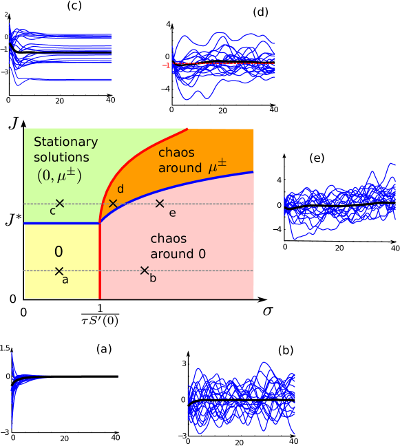
Refer to caption
Figure 2: Behavior of a one-population system with non-centered synaptic coefficients. Center: Bifurcation diagram (hand-drawn) segmented into four regions: two regions of stationary behavior (yellow: centered at zero and green: centered on μ±superscript𝜇plus-or-minus\mu^{\pm}) and two chaotic regions (pink: centered around zero and orange: centered around μ±superscript𝜇plus-or-minus\mu^{\pm}). The boundaries of these regions are: a pitchfork bifurcation (blue curve) separating the stationary or chaotic regions centered on 00 to the ones centered on μ±superscript𝜇plus-or-minus\mu^{\pm}, and a generalized SCS phase transition (red curve) separating the stationary and chaotic regimes. The subfigures (a)-(e) show the time course of 303030 arbitrarily chosen neurons in the network corresponding to the points a-e of the diagram: τ=1𝜏1\tau=1, S(0)=1superscript𝑆01S^{\prime}(0)=1, (a): J=0.5𝐽0.5J=0.5, σ=0.5𝜎0.5\sigma=0.5, (b): J=0.5𝐽0.5J=0.5, σ=1.5𝜎1.5\sigma=1.5, (c): J=1.5𝐽1.5J=1.5, σ=1.5𝜎1.5\sigma=1.5, (d): J=1.5𝐽1.5J=1.5, σ=1.7𝜎1.7\sigma=1.7, (e): J=1.5𝐽1.5J=1.5, σ=2𝜎2\sigma=2.

4.2.2 Delay-induced oscillations

We now consider a one-population network with delays. Without loss of generality, we consider that the time constant is equal to 111. The solutions of the mean-field equations with no heterogeneity are Gaussian processes whose moments reduce to a dynamical system:

{μ˙=μ+Jf(μ(tτ),v(tτ))v˙=2v+λ2cases˙𝜇absent𝜇𝐽𝑓𝜇𝑡𝜏𝑣𝑡𝜏˙𝑣absent2𝑣superscript𝜆2\begin{cases}\dot{\mu}&=-\mu+Jf(\mu(t-\tau),v(t-\tau))\\ \dot{v}&=-2\,v+\lambda^{2}\end{cases}

and hence the variance converges towards λ2/2superscript𝜆22\lambda^{2}/2. To fix ideas, we consider S(x)=erf(gx)𝑆𝑥erf𝑔𝑥S(x)=\text{erf}(gx), so that f(x,σ)=erf(gx1+g2Γ(σ))𝑓𝑥𝜎erf𝑔𝑥1superscript𝑔2Γ𝜎f(x,\sigma)=\text{erf}(\frac{g\,x}{\sqrt{1+g^{2}\Gamma(\sigma)}}). Since for any v𝑣v, f(0,v)=0𝑓0𝑣0f(0,v)=0, the null mean is a stationary solution of the equation. Its stability depends on the roots of the characteristic equation (or dispersion relationship):

ξ=1+Jfμ|0,λ22eξτ=1+Jg1+g2λ22eξτ.𝜉1evaluated-at𝐽𝑓𝜇0superscript𝜆22superscript𝑒𝜉𝜏1𝐽𝑔1superscript𝑔2superscript𝜆22superscript𝑒𝜉𝜏\xi=-1+J\left.\frac{\partial f}{\partial\mu}\right|_{0,\frac{\lambda^{2}}{2}}e^{-\xi\tau}=-1+J\frac{g}{\sqrt{1+g^{2}\frac{\lambda^{2}}{2}}}e^{-\xi\tau}.

If all characteristic roots have negative real part, the fixed point μ=0𝜇0\mu=0 is stable. As a function of the parameters of the system, characteristic roots can cross the imaginary axis and yield a destabilization of the fixed point. Turing-Hopf instabilities arise when there exists purely imaginary characteristic roots ξ=𝐢ω𝜉𝐢𝜔\xi=\mathbf{i}\omega. In that case, we obtain the following equivalent system:

{1+Jg1+g2λ22cos(ωτ)=0ω=Jg1+g2λ22sin(ωτ)cases1𝐽𝑔1superscript𝑔2superscript𝜆22𝜔𝜏0otherwise𝜔𝐽𝑔1superscript𝑔2superscript𝜆22𝜔𝜏otherwise\begin{cases}-1+J\frac{g}{\sqrt{1+g^{2}\frac{\lambda^{2}}{2}}}\cos(\omega\tau)=0\\ \omega=-J\frac{g}{\sqrt{1+g^{2}\frac{\lambda^{2}}{2}}}\sin(\omega\tau)\end{cases}

which has real solutions only for Jg1+g2λ22>1𝐽𝑔1superscript𝑔2superscript𝜆221J\frac{g}{\sqrt{1+g^{2}\frac{\lambda^{2}}{2}}}>1. It is then easy to show that Turing-Hopf bifurcations arise when the parameters satisfy the relationship:

τ=arccos(1+g2λ22Jg)J2g21+g2λ221𝜏1superscript𝑔2superscript𝜆22𝐽𝑔superscript𝐽2superscript𝑔21superscript𝑔2superscript𝜆221\tau=\frac{\arccos\left(\frac{\sqrt{1+g^{2}\frac{\lambda^{2}}{2}}}{Jg}\right)}{\sqrt{\frac{J^{2}g^{2}}{1+g^{2}\frac{\lambda^{2}}{2}}-1}}

and these correspond to characteristic roots ω=J2g21+g2λ221𝜔superscript𝐽2superscript𝑔21superscript𝑔2superscript𝜆221\omega=\sqrt{\frac{J^{2}g^{2}}{1+g^{2}\frac{\lambda^{2}}{2}}-1}. These result into oscillations of the solutions at a pulsation equal by ω𝜔\omega.

Let us now return to the case of random coefficients with variance σ𝜎\sigma and no additive noise λ=0𝜆0\lambda=0. The mean of the Gaussian solution satisfy the same equation as the one studied above with λ=Γ(σ)𝜆Γ𝜎\lambda=\Gamma(\sigma), and as noted in the previous section, the stationary covariance is an increasing function of σ𝜎\sigma. For J>fμ(0,0)𝐽𝑓𝜇00J>\frac{\partial f}{\partial\mu}(0,0), the fixed point 00 is unstable, and the covariance is non-zero. This implies that for sufficiently large values of the delay, the network displays oscillations. Thanks to the propagation of chaos property, all neurons have the same distribution, which is a Gaussian with oscillatory mean, and hence the network displays phase-locked oscillations. Eventually, as noise is increased beyond a critical value, a SCS phase transition occurs and the system no more displays phase locked oscillations but asynchronous chaotic activity. This is illustrated in figure Fig. 3
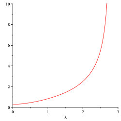
Refer to caption
(a) Turing-Hopf bifurcation curve
Refer to caption
(b) τ=0.1,σ=0.5formulae-sequence𝜏0.1𝜎0.5\tau=0.1,\;\sigma=0.5
Refer to caption
(c) τ=0.5,σ=0.5formulae-sequence𝜏0.5𝜎0.5\tau=0.5,\;\sigma=0.5
Refer to caption
(d) τ=0.5,σ=1formulae-sequence𝜏0.5𝜎1\tau=0.5,\;\sigma=1
Figure 3: One population delayed system, τ=1𝜏1\tau=1, S(x)=erf(gx)𝑆𝑥erf𝑔𝑥S(x)=\text{erf}(gx), g=3𝑔3g=3 and J=2𝐽2J=-2. (a) represents the curve of Turing-Hopf bifurcations in the plane (τ,λ)𝜏𝜆(\tau,\lambda) obtained analytically. (b): τ𝜏\tau small: no oscillations. As the delays are increased, a Turing Hopf bifurcation occurs and oscillations appear (b), which disappear when the heterogeneity σ𝜎\sigma is increased beyond a critical value in favor a chaotic activity (c).

4.3 Multi-population networks

In this section, we analyze the dynamics of randomly coupled neuronal networks in the case of the deterministic coupling of several original SCS networks, before turning the analysis of the dynamics of a more biologically plausible neuronal network composed of an excitatory and an inhibitory population. As demonstrated by Sompolinsky and coworkers in sompolinsky-crisanti-etal:88 , the study of the stationary states using equations (21) is very useful to analyze the dynamics of their networks. Unfortunately, this method does not persists in higher dimensions, since the equation does not necessarily derive from a potential. Indeed, in order for the equation to derive from a potential ΦM:M:subscriptΦ𝑀maps-tosuperscript𝑀\Phi_{M}:\mathbbm{R}^{M}\mapsto\mathbbm{R} in dimension M𝑀M greater than 111, we need that for any α{1,,M}𝛼1𝑀\alpha\in\{1,\ldots,M\}:

ΦMCα=Cα+β=1Mσαβ2ΔβsubscriptΦ𝑀superscript𝐶𝛼superscript𝐶𝛼superscriptsubscript𝛽1𝑀superscriptsubscript𝜎𝛼𝛽2superscriptΔ𝛽\frac{\partial\Phi_{M}}{\partial C^{\alpha}}=-C^{\alpha}+\sum_{\beta=1}^{M}\sigma_{\alpha\beta}^{2}\Delta^{\beta}

The only case where this is possible is the case where σαβ2=0superscriptsubscript𝜎𝛼𝛽20\sigma_{\alpha\beta}^{2}=0 for any αβ𝛼𝛽\alpha\neq\beta. Indeed, shall the above relationship be true, the equality 2ΦMCαCβ=2ΦMCβCαsuperscript2subscriptΦ𝑀superscript𝐶𝛼superscript𝐶𝛽superscript2subscriptΦ𝑀superscript𝐶𝛽superscript𝐶𝛼\frac{\partial^{2}\Phi_{M}}{\partial C^{\alpha}\partial C^{\beta}}=\frac{\partial^{2}\Phi_{M}}{\partial C^{\beta}\partial C^{\alpha}} directly yields σαβ2ΔβCβ=σβα2ΔαCαsuperscriptsubscript𝜎𝛼𝛽2superscriptΔ𝛽superscript𝐶𝛽superscriptsubscript𝜎𝛽𝛼2superscriptΔ𝛼superscript𝐶𝛼\sigma_{\alpha\beta}^{2}\frac{\partial\Delta^{\beta}}{\partial C^{\beta}}=\sigma_{\beta\alpha}^{2}\frac{\partial\Delta^{\alpha}}{\partial C^{\alpha}}. The lefthand side is a function of Cαsuperscript𝐶𝛼C^{\alpha} only and the righthand side a function of Cβsuperscript𝐶𝛽C^{\beta} only, they for αβ𝛼𝛽\alpha\neq\beta these functions are necessarily constant. For regular functions S𝑆S, this necessitates to have σαβ=σβα=0subscript𝜎𝛼𝛽subscript𝜎𝛽𝛼0\sigma_{\alpha\beta}=\sigma_{\beta\alpha}=0. This is precisely the case of deterministic lateral connections between randomly coupled networks, which will now study.

4.3.1 Deterministic lateral coupling of SCS networks

In this section we analyze the coupling of different SCS networks, called lateral coupling, with deterministic coefficients. The only randomness in the models is included in the random synaptic coefficients between neurons belonging to the same population. In that particular case, equation (23) derives from the potential ΦM(C1CM)=α=1MΦ1(Cα)subscriptΦ𝑀superscript𝐶1superscript𝐶𝑀superscriptsubscript𝛼1𝑀subscriptΦ1superscript𝐶𝛼\Phi_{M}(C^{1}\cdots C^{M})=\sum_{\alpha=1}^{M}\Phi_{1}(C^{\alpha}), and in that case the analysis driven by Sompolinsky and collaborators can be adapted to the multi-dimensional case. Since the potential is now the sum of the individual potentials at each population, we observe a strange phenomenon of localization of chaos in the populations that display a large heterogeneity (namely, in our notations, when the SCS condition σαα2Sαα(0)τα>1superscriptsubscript𝜎𝛼𝛼2subscriptsuperscript𝑆𝛼𝛼0subscript𝜏𝛼1\sigma_{\alpha\alpha}^{2}S^{\prime}_{\alpha\alpha}(0)\tau_{\alpha}>1 is satisfied). Only the populations that individually would be in a chaotic state are in a chaotic state, and the other populations converge to zero with a Dirac delta covariance at zero, and the input received by such populations from chaotic populations do not perturb this state. Let us for instance illustrate this phenomenon on a two-populations network with parameters:

J¯=(0J21J120)andσ=(σ100σ2)formulae-sequence¯𝐽0subscript𝐽21subscript𝐽120and𝜎subscript𝜎100subscript𝜎2\bar{J}=\left(\begin{array}[]{cc}0&J_{21}\\ J_{12}&0\end{array}\right)\qquad\text{and}\qquad\sigma=\left(\begin{array}[]{cc}\sigma_{1}&0\\ 0&\sigma_{2}\end{array}\right)

Each population receives input from the neurons of the other population, with a constant synaptic weight equal to Jαβsubscript𝐽𝛼𝛽J_{\alpha\beta}, and the intra-population synaptic weights are noisy.
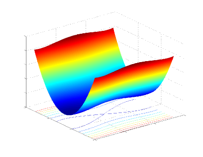
Refer to caption
(a) Shape of the potential
Refer to caption
(b) Trajectories
Figure 4: Dynamics for a 2-populations network with Hamiltonian dynamics (no variance on the cross-population synaptic weights): τ1=τ2=1subscript𝜏1subscript𝜏21\tau_{1}=\tau_{2}=1, σ1=3>1subscript𝜎131\sigma_{1}=3>1, σ2=0.5<1subscript𝜎20.51\sigma_{2}=0.5<1, J12=J21=3subscript𝐽12𝐽213J_{12}=J21=3. The potential shows a double-well shape, corresponding to a chaotic state on population 1 and a stationary state on population 2. Simulation of a 4 00040004\,000 neurons network illustrate this phenomenon (right): blue (resp. red): 303030 arbitrarily chosen trajectories population from 1 (resp. 2).

Further analysis of this networks as a function of the coupling reveals a similar phenomenon as the one described in the one-population network of section 4.2.1. Indeed, as the strength of the lateral coupling J12subscript𝐽12J_{12} and J21subscript𝐽21J_{21} are increased, additional stationary solutions with non-zero covariance appear. Let us for instance denote by μsuperscript𝜇\mu^{*} the mean of one of these stationary solutions. Following SCS analysis, we are ensured that the behavior of the trajectories of neurons in population α𝛼\alpha around μαsubscriptsuperscript𝜇𝛼\mu^{*}_{\alpha} is stationary as long as σα<1ταS(μα)subscript𝜎𝛼1subscript𝜏𝛼superscript𝑆subscriptsuperscript𝜇𝛼\sigma_{\alpha}<\frac{1}{\tau_{\alpha}S^{\prime}(\mu^{*}_{\alpha})} and chaotic otherwise, and this independently of the behavior of the other population. This phenomenon is illustrated in figure Fig. 5.
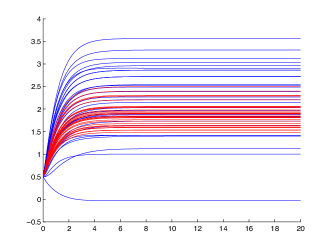
Refer to caption
(a) Stationary States
Refer to caption
(b) Localized Chaos
Figure 5: Stationary and partially chaotic solutions of a two populations network with deterministic lateral around non-zero fixed points. J12=J21=4subscript𝐽12subscript𝐽214J_{12}=J_{21}=4, σ2=0.5subscript𝜎20.5\sigma_{2}=0.5, (left): σ1=2subscript𝜎12\sigma_{1}=2: both populations display a stationary behavior, (right): σ1=5subscript𝜎15\sigma_{1}=5: only population 1 is chaotic and the irregularity is not transmitted to population 2.

4.4 Heterogeneity-induced oscillations in two-populations networks

We eventually discuss the effect of heterogeneities in a more biologically plausible neuronal network including one excitatory and one inhibitory population, with strictly positive sigmoidal transforms (since these functions model the input to firing-rate transformation), that tend to zero at -\infty and to 111 at \infty. This system was analyzed in touboul-hermann:12 . Considering M=2𝑀2M=2 populations, all sigmoids equal to erf(gx)=gxey2/2/2π𝑑yerf𝑔𝑥superscriptsubscript𝑔𝑥superscript𝑒superscript𝑦222𝜋differential-d𝑦\text{erf}(gx)=\int_{-\infty}^{gx}e^{-y^{2}/2}/\sqrt{2\pi}\,dy (yielding fαβ(x,v)=erf(gx/1+g2v)subscript𝑓𝛼𝛽𝑥𝑣erf𝑔𝑥1superscript𝑔2𝑣f_{\alpha\beta}(x,v)=\text{erf}(gx/\sqrt{1+g^{2}v})), all time constants θα=1subscript𝜃𝛼1\theta_{\alpha}=1, and the connectivity matrix, inspired from the seminal article of Wilson and Cowan wilson-cowan:72 :

J¯=(1512165).¯𝐽1512165\bar{J}=\left(\begin{array}[]{cc}15&-12\\ 16&-5\end{array}\right).

we showed that the system presents phase transitions as a function of the heterogeneity parameter, between stationary distributions to periodic oscillations (see figure Fig. 6): considering all σαβsubscript𝜎𝛼𝛽\sigma_{\alpha\beta} equal and denoting σ𝜎\sigma the common value, we observe that for small heterogeneity parameter σ𝜎\sigma, the network converges towards a stationary solution with non-zero mean. For intermediate values of the heterogeneity, phase-locked perfectly periodic behaviors appear at the network level, that disappear, as heterogeneity is further increased, through a SCS phase transition yielding chaotic activity.
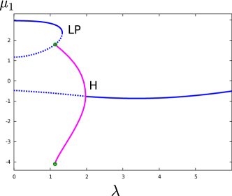
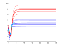
Refer to caption
(a) Bifurcation Diagram
Refer to caption
(b) σ=0.9𝜎0.9\sigma=0.9
Refer to caption
(c) σ=1.6𝜎1.6\sigma=1.6
Refer to caption
(d) σ=3.5𝜎3.5\sigma=3.5
Figure 6: Heterogeneity-induced oscillations in a two populations excitatory-inhibitory network. (a) Bifurcation diagram of the system of ODEs (19) as a function of a presumably constant common value Γ(σ)Γ𝜎\Gamma(\sigma). LP: saddle-node bifurcation, H: Hopf bifurcation, Sh: Saddle-homoclinic bifurcation, blue: fixed points (solid: stable, dashed: unstable), magenta: limit cycles. (b)-(d): simulations of the heterogeneous network with 2 00020002\,000 neurons per population, for increasing values of the heterogeneity parameter σ𝜎\sigma displays a transition from stationary to periodic phase-locked behaviors, and then to chaotic behavior. blue (resp. red): 30 arbitrary trajectories of population 1 (resp. 2), cyan (resp. magenta): average on all neurons of population 1 (resp. 2).

This phenomenon relates the level of heterogeneity to the presence of synchronized oscillations in networks, an essential phenomenon, as we discuss in the conclusion.

5 Discussion

In this manuscript, we analyzed randomly coupled neuronal networks and derived their limit as the number of neurons tends to infinity. To this purpose, we showed that the system satisfied a large deviation principle and exhibited the related good rate function. This approach generalized the work of Gerard Ben Arous and Alice Guionnet ben-arous-guionnet:95 ; guionnet:97 developed for spin glasses in three main directions: (i) the synaptic weights are not centered, introducing additional, deterministic terms in the coupling, (ii) interactions are delayed, which projects the problem into infinite dimensions, and (iii) the system is composed of several populations, which was handled showing that empirical measures on each populations simultaneously satisfy a large deviation principle. The proof is made on a particular model very popular in physics and neurosciences, the Wilson and Cowan system, which is close of the famous Hopfield model, but as mentioned, can be easily generalized to nonlinear neuron models. Indeed, most of the proofs deal a quantity which is related to the density of the coupled network with respect to the uncoupled dynamics, and this quantity is independent of the dynamics of individual cells. Our approach can be also readily extended to networks with distributed delays. Eventually, let us note that this result provides large-deviations estimates on the convergence of deterministically coupled networks as studied in touboul-hermann-faugeras:11 .

From the neuroscience viewpoint, this approach has the interest to justify an equation which has been widely used in the analysis of large-scale networks, and introduced in the seminal paper of Sompolinsky and collaborators sompolinsky-crisanti-etal:88 . Moreover, our setting substantially extends their result by taking into account important features present in cortical networks: interconnection delays, multiple populations with non-zero average synaptic connection. All these refinements allowed going deeper into the understanding of the dynamics of neuronal networks. In particular, we showed that delays can induce oscillations in one-populations networks modulated by the level of heterogeneity, and that non-zero average connectivity yields non-trivial dynamics that were not present in the original SCS model. Moreover, we showed that networks with multiple populations can show relative counter-intuitive phenomena such as the localization of chaos: a few populations can have a chaotic behavior which is not transmitted to the other populations, whatever the connection strength. Another phenomenon we illustrated was the apparition of heterogeneity-induced oscillations, phenomenon first presented in a very recent article touboul-hermann:12 . As discussed in that article, the latter phenomenon can be related to experimental studies that showed that the cortex of developing rats subject to absence seizures (abnormal synchronization of some cortical areas) was characterized by the same mean synaptic connectivity, but increased dispersion of the synaptic weights aradi-soltesz:02 . We further showed here that such oscillations were facilitated by the presence of delays. Let us eventually underline that the particular form of our system is not essential in the apparition of such phenomena, and in touboul-hermann:12 , it is shown that the transition to synchronized activity as a function of heterogeneity levels persists for realistic neuronal networks made of excitable cells, the Fitzhugh-Nagumo model.

An important observations is that in all the examples treated, the SCS phase transition to chaos is present as the heterogeneity is increased. This phenomenon seems relatively universal in this kind of randomly coupled neuronal networks. It was very recently related to the topological complexity of the underlying vector field in wainrib-touboul:2012 in the original SCS framework, and we conjecture that the same phenomenon occurs in our more complex settings.

The analysis of the present manuscript underlines the fact that the structure of connectivity maps is essential to the function of the networks, and illustrated the fact that averaging effects do not cancel the structure into populations and allow serving functions such as oscillations. However, actual brain connectivity maps are not recurrent, and can display different topologies, with different computational capabilities. The extension of our methods to such networks is an active part of our future research. Moreover, our analysis did not take into account the plasticity mechanisms, resulting in the slow evolution of the synaptic weights as a function of the activity of neurons, which tends to correlate the synaptic weights to the voltage variables. Techniques to rigorously address the dynamics of neuronal networks with non-recurrent connectivity, with specific topologies, or with correlated synaptic weights, are deep questions that are still largely left unexplored, and we can expect that a wide range of novel phenomena will arise from the analysis of such networks.

Appendix A Proofs

A.1 Proof of Lemma 1

This appendix is the proof of lemma 1 concerned with the properties of the functions used in our large deviation principle in a discrete time framework.

Proof

Before proceeding to the proof of the lemma, let us start by showing an inequality which will be very useful in several steps of the demonstration. We recall the following well known formula (see (deuschel-stroock:89, , Lemma 3.2.13) for instance):

I(μ|P)=sup(𝒞Φ𝑑μlog𝒞expΦdP;Φ𝒞b(𝒞))𝐼conditional𝜇𝑃supremumsubscript𝒞Φdifferential-d𝜇subscript𝒞Φ𝑑𝑃Φsubscript𝒞𝑏𝒞I(\mu|P)=\sup\left(\int_{\mathcal{C}}\Phi d\mu-\log\int_{\mathcal{C}}\exp\Phi dP\;;\;\Phi\in\mathcal{C}_{b}(\mathcal{C})\right)

so that, for any bounded measurable function ΦΦ\Phi on 𝒞𝒞\mathcal{C}, we have:

𝒞Φ𝑑μI(μ|P)+log𝒞expΦdPsubscript𝒞Φdifferential-d𝜇𝐼conditional𝜇𝑃subscript𝒞Φ𝑑𝑃\int_{\mathcal{C}}\Phi d\mu\leq I(\mu|P)+\log\int_{\mathcal{C}}\exp\Phi dP (24)

The result hold for positive measurable functions by the monotone convergence theorem.

Proof of Lemma 1.(i).
Lets prove the lipschitzianity result for Γ1α,ksubscriptsuperscriptΓ𝛼𝑘1\Gamma^{\alpha,k}_{1}. We have:

|log(1+\displaystyle\Big{|}\log\Big{(}1+ exp(12l=0kGtlα2(tl+1tl))d(γKμγKν)exp(12l=0kGtlα2(tl+1tl))𝑑γKν)|=|Γ1α,k(μ)Γ1α,k(ν)+12((mμα)2(mνα)2)(t(k))dt|\displaystyle\frac{\int\exp\big{(}-\frac{1}{2}\sum_{l=0}^{k}{G^{\alpha}_{t_{l}}}^{2}(t_{l+1}-t_{l})\big{)}d(\gamma_{K_{\mu}}-\gamma_{K_{\nu}})}{\int\exp\big{(}-\frac{1}{2}\sum_{l=0}^{k}{G^{\alpha}_{t_{l}}}^{2}(t_{l+1}-t_{l})\big{)}d\gamma_{K_{\nu}}}\Big{)}\Big{|}=\Big{|}\Gamma_{1}^{\alpha,k}(\mu)-\Gamma_{1}^{\alpha,k}(\nu)+\frac{1}{2}\int((m^{\alpha}_{\mu})^{2}-(m^{\alpha}_{\nu})^{2})(t^{(k)})dt\Big{|}
exp{kαT2λα2}|exp(120TGt(k)α2𝑑t)d(γKμγKν)|absentsubscript𝑘𝛼𝑇2superscriptsubscript𝜆𝛼212superscriptsubscript0𝑇superscriptsubscriptsuperscript𝐺𝛼superscript𝑡𝑘2differential-d𝑡𝑑subscript𝛾subscript𝐾𝜇subscript𝛾subscript𝐾𝜈\displaystyle\leq\exp\Big{\{}\frac{k_{\alpha}T}{2\lambda_{\alpha}^{2}}\Big{\}}\Big{|}\int\exp\big{(}-\frac{1}{2}\int_{0}^{T}{G^{\alpha}_{t^{(k)}}}^{2}dt\big{)}d(\gamma_{K_{\mu}}-\gamma_{K_{\nu}})\Big{|}

Let ξ𝜉\xi be a probability measure on 𝒞×𝒞𝒞𝒞\mathcal{C}\times\mathcal{C} with marginals μ𝜇\mu and ν𝜈\nu, and let γξsubscript𝛾𝜉\gamma_{\xi} be the law of a bidimensional centered gaussian process (Gα,Gα~)superscript𝐺𝛼~superscript𝐺𝛼(G^{\alpha},\widetilde{G^{\alpha}}) with covariance Kξαsubscriptsuperscript𝐾𝛼𝜉K^{\alpha}_{\xi}:

Kξα(s,t)=γ=1Mσαγ2λα2(Sαγ(xsταγγ)Sαγ(xtταγγ)𝑑ξ(x,y)Sαγ(xsταγγ)Sαγ(ytταγγ)𝑑ξ(x,y)Sαγ(ysταγγ)Sαγ(xtταγγ)𝑑ξ(x,y)Sαγ(ysταγγ)Sαγ(ytταγγ)𝑑ξ(x,y)),subscriptsuperscript𝐾𝛼𝜉𝑠𝑡superscriptsubscript𝛾1𝑀superscriptsubscript𝜎𝛼𝛾2superscriptsubscript𝜆𝛼2subscript𝑆𝛼𝛾subscriptsuperscript𝑥𝛾𝑠subscript𝜏𝛼𝛾subscript𝑆𝛼𝛾subscriptsuperscript𝑥𝛾𝑡subscript𝜏𝛼𝛾differential-d𝜉𝑥𝑦subscript𝑆𝛼𝛾subscriptsuperscript𝑥𝛾𝑠subscript𝜏𝛼𝛾subscript𝑆𝛼𝛾subscriptsuperscript𝑦𝛾𝑡subscript𝜏𝛼𝛾differential-d𝜉𝑥𝑦missing-subexpressionsubscript𝑆𝛼𝛾subscriptsuperscript𝑦𝛾𝑠subscript𝜏𝛼𝛾subscript𝑆𝛼𝛾subscriptsuperscript𝑥𝛾𝑡subscript𝜏𝛼𝛾differential-d𝜉𝑥𝑦subscript𝑆𝛼𝛾subscriptsuperscript𝑦𝛾𝑠subscript𝜏𝛼𝛾subscript𝑆𝛼𝛾subscriptsuperscript𝑦𝛾𝑡subscript𝜏𝛼𝛾differential-d𝜉𝑥𝑦missing-subexpressionK^{\alpha}_{\xi}(s,t)=\sum_{\gamma=1}^{M}\frac{\sigma_{\alpha\gamma}^{2}}{\lambda_{\alpha}^{2}}\left(\begin{array}[]{ccc}\int S_{\alpha\gamma}(x^{\gamma}_{s-\tau_{\alpha\gamma}})S_{\alpha\gamma}(x^{\gamma}_{t-\tau_{\alpha\gamma}})\,d\xi(x,y)&\int S_{\alpha\gamma}(x^{\gamma}_{s-\tau_{\alpha\gamma}})S_{\alpha\gamma}(y^{\gamma}_{t-\tau_{\alpha\gamma}})\,d\xi(x,y)\\ \int S_{\alpha\gamma}(y^{\gamma}_{s-\tau_{\alpha\gamma}})S_{\alpha\gamma}(x^{\gamma}_{t-\tau_{\alpha\gamma}})\,d\xi(x,y)&\int S_{\alpha\gamma}(y^{\gamma}_{s-\tau_{\alpha\gamma}})S_{\alpha\gamma}(y^{\gamma}_{t-\tau_{\alpha\gamma}})\,d\xi(x,y)\\ \end{array}\right), (25)

Then,

|exp(120TGt(k)α2𝑑t)d(γKμγKν)|=|{exp(120TGt(k)α2𝑑t)exp(120TGt(k)α~2𝑑t)}𝑑γξ|120T|Gt(k)α2Gt(k)α~2|𝑑t𝑑γξ12ε=±1(0T(Gt(k)α+εGt(k)α~)2𝑑t𝑑γξ)1212superscriptsubscript0𝑇superscriptsubscriptsuperscript𝐺𝛼superscript𝑡𝑘2differential-d𝑡𝑑subscript𝛾subscript𝐾𝜇subscript𝛾subscript𝐾𝜈12superscriptsubscript0𝑇superscriptsubscriptsuperscript𝐺𝛼superscript𝑡𝑘2differential-d𝑡12superscriptsubscript0𝑇superscript~subscriptsuperscript𝐺𝛼superscript𝑡𝑘2differential-d𝑡differential-dsubscript𝛾𝜉12superscriptsubscript0𝑇superscriptsubscriptsuperscript𝐺𝛼superscript𝑡𝑘2superscript~subscriptsuperscript𝐺𝛼superscript𝑡𝑘2differential-d𝑡differential-dsubscript𝛾𝜉12subscriptproduct𝜀plus-or-minus1superscriptsuperscriptsubscript0𝑇superscriptsubscriptsuperscript𝐺𝛼superscript𝑡𝑘𝜀~subscriptsuperscript𝐺𝛼superscript𝑡𝑘2differential-d𝑡differential-dsubscript𝛾𝜉12\Big{|}\int\exp\big{(}-\frac{1}{2}\int_{0}^{T}{G^{\alpha}_{t^{(k)}}}^{2}dt\big{)}d(\gamma_{K_{\mu}}-\gamma_{K_{\nu}})\Big{|}=\Big{|}\int\bigg{\{}\exp\big{(}-\frac{1}{2}\int_{0}^{T}{G^{\alpha}_{t^{(k)}}}^{2}dt\big{)}-\exp\big{(}-\frac{1}{2}\int_{0}^{T}\widetilde{G^{\alpha}_{t^{(k)}}}^{2}dt\big{)}\bigg{\}}d\gamma_{\xi}\Big{|}\\ \qquad\leq\frac{1}{2}\int\int_{0}^{T}\big{|}{G^{\alpha}_{t^{(k)}}}^{2}-\widetilde{G^{\alpha}_{t^{(k)}}}^{2}\big{|}dtd\gamma_{\xi}\\ \leq\frac{1}{2}\prod_{\varepsilon=\pm 1}\bigg{(}\int\int_{0}^{T}(G^{\alpha}_{t^{(k)}}+\varepsilon\widetilde{G^{\alpha}_{t^{(k)}}})^{2}dtd\gamma_{\xi}\bigg{)}^{\frac{1}{2}}

by Cauchy-Schwarz inequality. Then, using the covariance of (Gα,Gα~)superscript𝐺𝛼~superscript𝐺𝛼(G^{\alpha},\widetilde{G^{\alpha}}) under γξsubscript𝛾𝜉\gamma_{\xi}, we find:

|Γ1α,k(μ)Γ1α,k(ν)+12((mμα)2(mνα)2)(t(k))𝑑t|superscriptsubscriptΓ1𝛼𝑘𝜇superscriptsubscriptΓ1𝛼𝑘𝜈12superscriptsubscriptsuperscript𝑚𝛼𝜇2superscriptsubscriptsuperscript𝑚𝛼𝜈2superscript𝑡𝑘differential-d𝑡\displaystyle\Big{|}\Gamma_{1}^{\alpha,k}(\mu)-\Gamma_{1}^{\alpha,k}(\nu)+\frac{1}{2}\int((m^{\alpha}_{\mu})^{2}-(m^{\alpha}_{\nu})^{2})(t^{(k)})dt\Big{|} (26)
12exp{kαT2λα2}(4kαTλα2)12{1λα2γ=1Mσαγ20T(Sαγ(xtταγγ)Sαγ(ytταγγ))2𝑑t𝑑ξ(x,y)}12absent12subscript𝑘𝛼𝑇2superscriptsubscript𝜆𝛼2superscript4subscript𝑘𝛼𝑇superscriptsubscript𝜆𝛼212superscript1superscriptsubscript𝜆𝛼2superscriptsubscript𝛾1𝑀superscriptsubscript𝜎𝛼𝛾2superscriptsubscript0𝑇superscriptsubscript𝑆𝛼𝛾subscriptsuperscript𝑥𝛾𝑡subscript𝜏𝛼𝛾subscript𝑆𝛼𝛾subscriptsuperscript𝑦𝛾𝑡subscript𝜏𝛼𝛾2differential-d𝑡differential-d𝜉𝑥𝑦12\displaystyle\leq\frac{1}{2}\exp\Big{\{}\frac{k_{\alpha}T}{2\lambda_{\alpha}^{2}}\Big{\}}\Big{(}\frac{4k_{\alpha}T}{\lambda_{\alpha}^{2}}\Big{)}^{\frac{1}{2}}\bigg{\{}\frac{1}{\lambda_{\alpha}^{2}}\sum_{\gamma=1}^{M}\sigma_{\alpha\gamma}^{2}\int\int_{0}^{T}(S_{\alpha\gamma}(x^{\gamma}_{t-\tau_{\alpha\gamma}})-S_{\alpha\gamma}(y^{\gamma}_{t-\tau_{\alpha\gamma}}))^{2}dt\,d\xi(x,y)\bigg{\}}^{\frac{1}{2}}
kαλα2Texp{kαT2λα2}maxγ=1M{0T|Sαγ(xtταγγ)Sαγ(ytταγγ)|2dtdξ(x,y)}12\displaystyle\leq\frac{k_{\alpha}}{\lambda_{\alpha}^{2}}\sqrt{T}\exp\Big{\{}\frac{k_{\alpha}T}{2\lambda_{\alpha}^{2}}\Big{\}}\max_{\gamma=1\cdots M}\bigg{\{}\int\int_{0}^{T}\big{|}S_{\alpha\gamma}(x^{\gamma}_{t-\tau_{\alpha\gamma}})-S_{\alpha\gamma}(y^{\gamma}_{t-\tau_{\alpha\gamma}})\big{|}^{2}dt\,d\xi(x,y)\bigg{\}}^{\frac{1}{2}} (27)

Moreover, we have:

|mμα(t(k))2mνα(t(k))2dt|subscriptsuperscript𝑚𝛼𝜇superscriptsuperscript𝑡𝑘2subscriptsuperscript𝑚𝛼𝜈superscriptsuperscript𝑡𝑘2𝑑𝑡\displaystyle\Big{|}\int{m^{\alpha}_{\mu}(t^{(k)})}^{2}-{m^{\alpha}_{\nu}(t^{(k)})}^{2}dt\Big{|} =|(mμα(t(k))mνα(t(k)))(mμα(t(k))+mνα(t(k)))|𝑑tabsentsubscriptsuperscript𝑚𝛼𝜇superscript𝑡𝑘subscriptsuperscript𝑚𝛼𝜈superscript𝑡𝑘subscriptsuperscript𝑚𝛼𝜇superscript𝑡𝑘subscriptsuperscript𝑚𝛼𝜈superscript𝑡𝑘differential-d𝑡\displaystyle=\int\Big{|}\Big{(}m^{\alpha}_{\mu}(t^{(k)})-m^{\alpha}_{\nu}(t^{(k)})\Big{)}\Big{(}m^{\alpha}_{\mu}(t^{(k)})+m^{\alpha}_{\nu}(t^{(k)})\Big{)}\Big{|}dt
2J¯αλα|mμα(t(k))mνα(t(k))|𝑑tabsent2subscript¯𝐽𝛼subscript𝜆𝛼subscriptsuperscript𝑚𝛼𝜇superscript𝑡𝑘subscriptsuperscript𝑚𝛼𝜈superscript𝑡𝑘differential-d𝑡\displaystyle\leq 2\frac{\bar{J}_{\alpha}}{\lambda_{\alpha}}\int\big{|}m^{\alpha}_{\mu}(t^{(k)})-m^{\alpha}_{\nu}(t^{(k)})\big{|}dt

But

0T|(mμαmνα)(t)|𝑑tsuperscriptsubscript0𝑇subscriptsuperscript𝑚𝛼𝜇subscriptsuperscript𝑚𝛼𝜈𝑡differential-d𝑡\displaystyle\int_{0}^{T}|(m^{\alpha}_{\mu}-m^{\alpha}_{\nu})(t)|dt =0T|1λαγ=1MJ¯αγSαγ(xtτγ)d(μν)(x)|𝑑tabsentsuperscriptsubscript0𝑇1subscript𝜆𝛼superscriptsubscript𝛾1𝑀subscript¯𝐽𝛼𝛾subscript𝑆𝛼𝛾subscriptsuperscript𝑥𝛾𝑡𝜏𝑑𝜇𝜈𝑥differential-d𝑡\displaystyle=\int_{0}^{T}\Big{|}\frac{1}{\lambda_{\alpha}}\sum_{\gamma=1}^{M}\bar{J}_{\alpha\gamma}\int S_{\alpha\gamma}(x^{\gamma}_{t-{\tau}})d(\mu-\nu)(x)\Big{|}\,dt
1λαγ=1M|J¯αγ|0T|Sαγ(xtταγγ)d(μν)(x)|𝑑tabsent1subscript𝜆𝛼superscriptsubscript𝛾1𝑀subscript¯𝐽𝛼𝛾superscriptsubscript0𝑇subscript𝑆𝛼𝛾subscriptsuperscript𝑥𝛾𝑡subscript𝜏𝛼𝛾𝑑𝜇𝜈𝑥differential-d𝑡\displaystyle\leq\frac{1}{\lambda_{\alpha}}\sum_{\gamma=1}^{M}|\bar{J}_{\alpha\gamma}|\>\int_{0}^{T}\Big{|}\int S_{\alpha\gamma}(x^{\gamma}_{t-{\tau_{\alpha\gamma}}})d(\mu-\nu)(x)\Big{|}\,dt
1λαγ=1M|J¯αγ|0T|Sαγ(xtταγγ)Sαγ(ytτγ)|𝑑t𝑑ξ(x,y)absent1subscript𝜆𝛼superscriptsubscript𝛾1𝑀subscript¯𝐽𝛼𝛾superscriptsubscript0𝑇subscript𝑆𝛼𝛾subscriptsuperscript𝑥𝛾𝑡subscript𝜏𝛼𝛾subscript𝑆𝛼𝛾subscriptsuperscript𝑦𝛾𝑡𝜏differential-d𝑡differential-d𝜉𝑥𝑦\displaystyle\leq\frac{1}{\lambda_{\alpha}}\sum_{\gamma=1}^{M}|\bar{J}_{\alpha\gamma}|\>\int\int_{0}^{T}|S_{\alpha\gamma}(x^{\gamma}_{t-{\tau_{\alpha\gamma}}})-S_{\alpha\gamma}(y^{\gamma}_{t-{\tau}})|dt\,d\xi(x,y)
J¯αλαmaxγ=1M(0T|Sαγ(xtταγγ)Sαγ(ytτγ)|2dtdξ(x,y))12\displaystyle\leq\frac{\bar{J}_{\alpha}}{\lambda_{\alpha}}\max_{\gamma=1\cdots M}\Big{(}\int\int_{0}^{T}\big{|}S_{\alpha\gamma}(x^{\gamma}_{t-{\tau_{\alpha\gamma}}})-S_{\alpha\gamma}(y^{\gamma}_{t-{\tau}})\big{|}^{2}dt\,d\xi(x,y)\Big{)}^{\frac{1}{2}}

by Cauchy-Schwarz inequality.
Consequently:

|Γ1α,k(μ)Γ1α,k(ν)|(J¯α2λα2+kαλα2Texp{kαT2λα2})maxγ=1M(0T|Sαγ(xt(k)ταγγ)Sαγ(yt(k)ταγγ)|2dtdξ(x,y))12|\Gamma_{1}^{\alpha,k}(\mu)-\Gamma_{1}^{\alpha,k}(\nu)|\leq\big{(}\frac{\bar{J}_{\alpha}^{2}}{\lambda_{\alpha}^{2}}+\frac{k_{\alpha}}{\lambda_{\alpha}^{2}}\sqrt{T}\exp\Big{\{}\frac{k_{\alpha}T}{2\lambda_{\alpha}^{2}}\Big{\}}\big{)}\max_{\gamma=1\cdots M}\Big{(}\int\int_{0}^{T}\big{|}S_{\alpha\gamma}(x^{\gamma}_{t^{(k)}-\tau_{\alpha\gamma}})-S_{\alpha\gamma}(y^{\gamma}_{t^{(k)}-\tau_{\alpha\gamma}})\big{|}^{2}dt\,d\xi(x,y)\Big{)}^{\frac{1}{2}} (28)

As the Sαγsubscript𝑆𝛼𝛾S_{\alpha\gamma} are KSsubscript𝐾𝑆K_{S} Lipschitz, we have:

|Γ1α,k(μ)Γ1α,k(ν)|KST(J¯α2λα2+kαλα2Texp{kαT2λα2})dT(μ,ν),superscriptsubscriptΓ1𝛼𝑘𝜇superscriptsubscriptΓ1𝛼𝑘𝜈subscript𝐾𝑆𝑇superscriptsubscript¯𝐽𝛼2superscriptsubscript𝜆𝛼2subscript𝑘𝛼superscriptsubscript𝜆𝛼2𝑇subscript𝑘𝛼𝑇2superscriptsubscript𝜆𝛼2subscript𝑑𝑇𝜇𝜈|\Gamma_{1}^{\alpha,k}(\mu)-\Gamma_{1}^{\alpha,k}(\nu)|\leq K_{S}\sqrt{T}\big{(}\frac{\bar{J}_{\alpha}^{2}}{\lambda_{\alpha}^{2}}+\frac{k_{\alpha}}{\lambda_{\alpha}^{2}}\sqrt{T}\exp\Big{\{}\frac{k_{\alpha}T}{2\lambda_{\alpha}^{2}}\Big{\}}\big{)}d_{T}(\mu,\nu), (29)

so that Γ1α,ksuperscriptsubscriptΓ1𝛼𝑘\Gamma_{1}^{\alpha,k} is Lipschitz for the Vaserstein distance. Using the triangle inequality, the result holds for Γ1ksuperscriptsubscriptΓ1𝑘\Gamma_{1}^{k}.

Proof of Lemma1.(ii):
Let

Fμ(x)=log{exp{0T(𝐆t(k)(ω)+𝐦μ(t(k)))𝑑𝐖t(x)120T𝐆t(k)(ω)+𝐦μ(t(k))2𝑑t}𝑑γμ}.subscript𝐹𝜇𝑥superscriptsubscript0𝑇superscriptsubscript𝐆superscript𝑡𝑘𝜔subscript𝐦𝜇superscript𝑡𝑘differential-dsubscript𝐖𝑡𝑥12superscriptsubscript0𝑇superscriptnormsubscript𝐆superscript𝑡𝑘𝜔subscript𝐦𝜇superscript𝑡𝑘2differential-d𝑡differential-dsubscript𝛾𝜇F_{\mu}(x)=\log\bigg{\{}\int\exp\Big{\{}\int_{0}^{T}\big{(}\mathbf{G}_{t^{(k)}}(\omega)+\mathbf{m}_{\mu}(t^{(k)})\big{)}^{\prime}\cdot d\mathbf{W}_{t}(x)\\ -\frac{1}{2}\int_{0}^{T}\Big{\|}\mathbf{G}_{t^{(k)}}(\omega)+\mathbf{m}_{\mu}(t^{(k)})\Big{\|}^{2}dt\Big{\}}d\gamma_{\mu}\bigg{\}}.

This function is a.s. finite but not bounded, let us hence define for A+𝐴superscriptA\in\mathbbm{R}^{+}

FμA(x)=log{Aexp{0T(𝐆t(k)(ω)+𝐦μ(t(k)))𝑑𝐖t(x)120T𝐆t(k)(ω)+𝐦μ(t(k))2𝑑t}dγμ}.superscriptsubscript𝐹𝜇𝐴𝑥𝐴superscriptsubscript0𝑇superscriptsubscript𝐆superscript𝑡𝑘𝜔subscript𝐦𝜇superscript𝑡𝑘differential-dsubscript𝐖𝑡𝑥12superscriptsubscript0𝑇superscriptnormsubscript𝐆superscript𝑡𝑘𝜔subscript𝐦𝜇superscript𝑡𝑘2differential-d𝑡𝑑subscript𝛾𝜇F_{\mu}^{A}(x)=\log\bigg{\{}\int A\wedge\exp\Big{\{}\int_{0}^{T}\big{(}\mathbf{G}_{t^{(k)}}(\omega)+\mathbf{m}_{\mu}(t^{(k)})\big{)}^{\prime}\cdot d\mathbf{W}_{t}(x)\\ -\frac{1}{2}\int_{0}^{T}\Big{\|}\mathbf{G}_{t^{(k)}}(\omega)+\mathbf{m}_{\mu}(t^{(k)})\Big{\|}^{2}dt\Big{\}}d\gamma_{\mu}\bigg{\}}.

By the monotone convergence theorem and using equation (24), we have for any a1𝑎1a\geq 1:

aFμ(x)𝑑μ(x)I(μ|P)+log{expaFμ(x)𝑑P(x)}.𝑎subscript𝐹𝜇𝑥differential-d𝜇𝑥𝐼conditional𝜇𝑃𝑎subscript𝐹𝜇𝑥differential-d𝑃𝑥a\int F_{\mu}(x)d\mu(x)\leq I(\mu|P)+\log\bigg{\{}\int\exp{aF_{\mu}(x)}dP(x)\bigg{\}}.\\

By Jensen inequality and Fubini theorem,

exp(aFμ(x))𝑑P(x)𝑎subscript𝐹𝜇𝑥differential-d𝑃𝑥\displaystyle\int\exp{(aF_{\mu}(x)})dP(x) α=1Mexp{a0T(Gt(k)α+mμα(t(k)))𝑑Wtα(x)}𝑑Pα(x)absentsuperscriptsubscriptproduct𝛼1𝑀𝑎superscriptsubscript0𝑇subscriptsuperscript𝐺𝛼superscript𝑡𝑘subscriptsuperscript𝑚𝛼𝜇superscript𝑡𝑘differential-dsubscriptsuperscript𝑊𝛼𝑡𝑥differential-dsubscript𝑃𝛼𝑥\displaystyle\leq\int\prod_{\alpha=1}^{M}\int\exp\Big{\{}a\int_{0}^{T}\big{(}G^{\alpha}_{t^{(k)}}+m^{\alpha}_{\mu}(t^{(k)})\big{)}dW^{\alpha}_{t}(x)\Big{\}}dP_{\alpha}(x)
exp{a20T𝐆t(k)(ω)+𝐦μ(t(k))2𝑑t}dγμ.𝑎2superscriptsubscript0𝑇superscriptnormsubscript𝐆superscript𝑡𝑘𝜔subscript𝐦𝜇superscript𝑡𝑘2differential-d𝑡𝑑subscript𝛾𝜇\displaystyle\exp\Big{\{}-\frac{a}{2}\int_{0}^{T}\Big{\|}\mathbf{G}_{t^{(k)}}(\omega)+\mathbf{m}_{\mu}(t^{(k)})\Big{\|}^{2}dt\Big{\}}d\gamma_{\mu}.

But, as Wαsuperscript𝑊𝛼W^{\alpha} is a Pαsubscript𝑃𝛼P_{\alpha}-Brownian motion,

exp{a0T(Gt(k)α+mμα(t(k)))dWtα(x)}dPα(x)=exp{a220T(Gt(k)α+mμα(t(k)))2dt}].\int\exp\bigg{\{}a\int_{0}^{T}\big{(}G^{\alpha}_{t^{(k)}}+m^{\alpha}_{\mu}(t^{(k)})\big{)}dW^{\alpha}_{t}(x)\bigg{\}}dP_{\alpha}(x)=\exp\bigg{\{}\frac{a^{2}}{2}\int_{0}^{T}\big{(}G^{\alpha}_{t^{(k)}}+m^{\alpha}_{\mu}(t^{(k)})\big{)}^{2}dt\bigg{\}}\bigg{]}.\\

so that,

aFμ(x)𝑑μ(x)I(μ|P)+log{exp{a2a20T𝐆t(k)(ω)+𝐦μ(t(k))2𝑑t}𝑑γμ}.𝑎subscript𝐹𝜇𝑥differential-d𝜇𝑥𝐼conditional𝜇𝑃superscript𝑎2𝑎2superscriptsubscript0𝑇superscriptnormsubscript𝐆superscript𝑡𝑘𝜔subscript𝐦𝜇superscript𝑡𝑘2differential-d𝑡differential-dsubscript𝛾𝜇a\int F_{\mu}(x)d\mu(x)\leq I(\mu|P)+\log\bigg{\{}\int\exp\Big{\{}\frac{a^{2}-a}{2}\int_{0}^{T}\Big{\|}\mathbf{G}_{t^{(k)}}(\omega)+\mathbf{m}_{\mu}(t^{(k)})\Big{\|}^{2}dt\Big{\}}d\gamma_{\mu}\bigg{\}}.\\

Letting a=1𝑎1a=1 proves that ΓkI(|P)\Gamma^{k}\leq I(|P).

Proof of Lemma1 (iii):
As the components of 𝐆𝐆\mathbf{G} are independent under γμsubscript𝛾𝜇\gamma_{\mu}, we only have to check that, for every b>0𝑏0b>0, there exists a finite constant Cbsubscript𝐶𝑏C_{b} such that

μ[exp(b20T(Gsα+mμα(s))2𝑑s)]expbCbkαTλα2.subscript𝜇delimited-[]𝑏2superscriptsubscript0𝑇superscriptsubscriptsuperscript𝐺𝛼𝑠subscriptsuperscript𝑚𝛼𝜇𝑠2differential-d𝑠𝑏subscript𝐶𝑏subscript𝑘𝛼𝑇superscriptsubscript𝜆𝛼2{\mathcal{E}}_{\mu}\bigg{[}\exp{\Big{(}\frac{b}{2}\int_{0}^{T}\big{(}G^{\alpha}_{s}+m^{\alpha}_{\mu}(s)\big{)}^{2}ds\Big{)}}\bigg{]}\leq\exp{\frac{bC_{b}k_{\alpha}T}{\lambda_{\alpha}^{2}}}. (30)

It was proved in (ben-arous-guionnet:95, , Lemma A.3(2)) in their particular framework that for every b𝑏b verifying bkαTλα2<1𝑏subscript𝑘𝛼𝑇superscriptsubscript𝜆𝛼21\frac{bk_{\alpha}T}{\lambda_{\alpha}^{2}}<1, there exists a finite constant cbsubscript𝑐𝑏c_{b} such that:

exp(b20TGs2𝑑s)𝑑γμexpbcbkαTλα2.𝑏2superscriptsubscript0𝑇superscriptsubscript𝐺𝑠2differential-d𝑠differential-dsubscript𝛾𝜇𝑏subscript𝑐𝑏subscript𝑘𝛼𝑇superscriptsubscript𝜆𝛼2\int\exp{\Big{(}\frac{b}{2}\int_{0}^{T}G_{s}^{2}ds\Big{)}}d\gamma_{\mu}\leq\exp{\frac{bc_{b}k_{\alpha}T}{\lambda_{\alpha}^{2}}}.

In our case, the covariance function is slightly different of that of ben-arous-guionnet:95 , but the proof and result remain unchanged and can be readily extended.

Moreover, since we have

(Gsα+mμα(s))22Gsα2+2mμα(s)22Gsα2+2J¯α2λα2superscriptsubscriptsuperscript𝐺𝛼𝑠subscriptsuperscript𝑚𝛼𝜇𝑠22superscriptsubscriptsuperscript𝐺𝛼𝑠22subscriptsuperscript𝑚𝛼𝜇superscript𝑠22superscriptsubscriptsuperscript𝐺𝛼𝑠22superscriptsubscript¯𝐽𝛼2superscriptsubscript𝜆𝛼2\big{(}G^{\alpha}_{s}+m^{\alpha}_{\mu}(s)\big{)}^{2}\leq 2{G^{\alpha}_{s}}^{2}+2{m^{\alpha}_{\mu}(s)}^{2}\leq 2{G^{\alpha}_{s}}^{2}+2\frac{\bar{J}_{\alpha}^{2}}{\lambda_{\alpha}^{2}}

we obtain the desired result with the following constant Cb=2c2b+J¯α2kαsubscript𝐶𝑏2subscript𝑐2𝑏superscriptsubscript¯𝐽𝛼2subscript𝑘𝛼C_{b}=2c_{2b}+\frac{\bar{J}_{\alpha}^{2}}{k_{\alpha}}, under the condition 2bkαTλα2<12𝑏subscript𝑘𝛼𝑇superscriptsubscript𝜆𝛼21\frac{2bk_{\alpha}T}{\lambda_{\alpha}^{2}}<1.

Proof of Lemma1.(iv)
As above, lets prove the result for |Γ2,να,kΓ2α,k|subscriptsuperscriptΓ𝛼𝑘2𝜈subscriptsuperscriptΓ𝛼𝑘2\big{|}\Gamma^{\alpha,k}_{2,\nu}-\Gamma^{\alpha,k}_{2}\big{|}. We have:

|Γ2,να,k(μ)Γ2α,k(μ)|12|{(Gt(k)α(dWtαmμα(t(k))dt))2(Gt(k)α(dWtαmνα(t(k))dt))2}𝑑γK~μT,k𝑑μ|+12|(Gt(k)α(dWtαmνα(t(k))dt))2d(γK~νT,kγK~μT,k)𝑑μ|+|(mναmμα)(t(k))𝑑Wtα𝑑μ|superscriptsubscriptΓ2𝜈𝛼𝑘𝜇superscriptsubscriptΓ2𝛼𝑘𝜇12superscriptsubscriptsuperscript𝐺𝛼superscript𝑡𝑘𝑑subscriptsuperscript𝑊𝛼𝑡subscriptsuperscript𝑚𝛼𝜇superscript𝑡𝑘𝑑𝑡2superscriptsubscriptsuperscript𝐺𝛼superscript𝑡𝑘𝑑subscriptsuperscript𝑊𝛼𝑡subscriptsuperscript𝑚𝛼𝜈superscript𝑡𝑘𝑑𝑡2differential-dsubscript𝛾superscriptsubscript~𝐾𝜇𝑇𝑘differential-d𝜇12superscriptsubscriptsuperscript𝐺𝛼superscript𝑡𝑘𝑑subscriptsuperscript𝑊𝛼𝑡subscriptsuperscript𝑚𝛼𝜈superscript𝑡𝑘𝑑𝑡2𝑑subscript𝛾superscriptsubscript~𝐾𝜈𝑇𝑘subscript𝛾superscriptsubscript~𝐾𝜇𝑇𝑘differential-d𝜇subscriptsuperscript𝑚𝛼𝜈subscriptsuperscript𝑚𝛼𝜇superscript𝑡𝑘differential-dsubscriptsuperscript𝑊𝛼𝑡differential-d𝜇|\Gamma_{2,\nu}^{\alpha,k}(\mu)-\Gamma_{2}^{\alpha,k}(\mu)|\leq\frac{1}{2}\Big{|}\int\int\bigg{\{}\Big{(}\int G^{\alpha}_{t^{(k)}}(dW^{\alpha}_{t}-m^{\alpha}_{\mu}(t^{(k)})dt)\Big{)}^{2}-\Big{(}\int G^{\alpha}_{t^{(k)}}(dW^{\alpha}_{t}-m^{\alpha}_{\nu}(t^{(k)})dt)\Big{)}^{2}\bigg{\}}d\gamma_{\widetilde{K}_{\mu}^{T,k}}d\mu\Big{|}\\ +\frac{1}{2}\Big{|}\int\int\Big{(}\int G^{\alpha}_{t^{(k)}}(dW^{\alpha}_{t}-m^{\alpha}_{\nu}(t^{(k)})dt)\Big{)}^{2}d\big{(}\gamma_{\widetilde{K}_{\nu}^{T,k}}-\gamma_{\widetilde{K}_{\mu}^{T,k}}\big{)}d\mu|+|\int\int(m^{\alpha}_{\nu}-m^{\alpha}_{\mu})(t^{(k)})dW^{\alpha}_{t}d\mu\Big{|}

Let ξ𝜉\xi be a probability measure on 𝒞×𝒞𝒞𝒞\mathcal{C}\times\mathcal{C} with marginals μ𝜇\mu and ν𝜈\nu, and let γξsubscript𝛾𝜉\gamma_{\xi} be the law of a bidimensional centered gaussian process (Gα,Gα~)superscript𝐺𝛼~superscript𝐺𝛼(G^{\alpha},\widetilde{G^{\alpha}}) with covariance Kξαsubscriptsuperscript𝐾𝛼𝜉K^{\alpha}_{\xi}. Let

ΛTα,k(Gα)=exp(120TGt(k)α2𝑑t)exp(120TGt(k)α2𝑑t)𝑑γξ.superscriptsubscriptΛ𝑇𝛼𝑘superscript𝐺𝛼12superscriptsubscript0𝑇superscriptsubscriptsuperscript𝐺𝛼superscript𝑡𝑘2differential-d𝑡12superscriptsubscript0𝑇superscriptsubscriptsuperscript𝐺𝛼superscript𝑡𝑘2differential-d𝑡differential-dsubscript𝛾𝜉\Lambda_{T}^{\alpha,k}(G^{\alpha})=\frac{\exp{\bigg{(}-\frac{1}{2}\int_{0}^{T}{G^{\alpha}_{t^{(k)}}}^{2}dt\bigg{)}}}{\int\exp{\bigg{(}-\frac{1}{2}\int_{0}^{T}{G^{\alpha}_{t^{(k)}}}^{2}dt\bigg{)}}\,d\gamma_{\xi}}.

As in (ben-arous-guionnet:95, , lemma 3.4), we can show that:

|Γ2,να,k(μ)Γ2α,k(μ)|12|ΛTα,k(Gα)ΛTα,k(Gα~)|(Gt(k)α(dWtαmνα(t(k))dt))2𝑑γξ𝑑μB1+12ε=±1(ΛTα,k(Gα~)((Gt(k)α+εGα~t(k))(dWtαmνα(t(k))dt))2𝑑γξ𝑑μ)12B2+12|ΛTα,k(Gα){(Gt(k)α(dWtαmμα(t(k))dt))2(Gt(k)α(dWtαmνα(t(k))dt))2}𝑑γξ𝑑μ|B3+(|(mναmμα)(t(k))𝑑Wtα|2𝑑μ)12B4superscriptsubscriptΓ2𝜈𝛼𝑘𝜇superscriptsubscriptΓ2𝛼𝑘𝜇12superscriptsuperscriptsubscriptΛ𝑇𝛼𝑘superscript𝐺𝛼superscriptsubscriptΛ𝑇𝛼𝑘~superscript𝐺𝛼superscriptsubscriptsuperscript𝐺𝛼superscript𝑡𝑘𝑑subscriptsuperscript𝑊𝛼𝑡subscriptsuperscript𝑚𝛼𝜈superscript𝑡𝑘𝑑𝑡2differential-dsubscript𝛾𝜉differential-d𝜇subscript𝐵1subscript12subscriptproduct𝜀plus-or-minus1superscriptsuperscriptsubscriptΛ𝑇𝛼𝑘~superscript𝐺𝛼superscriptsubscriptsuperscript𝐺𝛼superscript𝑡𝑘𝜀subscript~superscript𝐺𝛼superscript𝑡𝑘𝑑subscriptsuperscript𝑊𝛼𝑡subscriptsuperscript𝑚𝛼𝜈superscript𝑡𝑘𝑑𝑡2differential-dsubscript𝛾𝜉differential-d𝜇12subscript𝐵212subscriptsuperscriptsubscriptΛ𝑇𝛼𝑘superscript𝐺𝛼superscriptsubscriptsuperscript𝐺𝛼superscript𝑡𝑘𝑑subscriptsuperscript𝑊𝛼𝑡subscriptsuperscript𝑚𝛼𝜇superscript𝑡𝑘𝑑𝑡2superscriptsubscriptsuperscript𝐺𝛼superscript𝑡𝑘𝑑subscriptsuperscript𝑊𝛼𝑡subscriptsuperscript𝑚𝛼𝜈superscript𝑡𝑘𝑑𝑡2differential-dsubscript𝛾𝜉differential-d𝜇subscript𝐵3subscriptsuperscriptsuperscriptsubscriptsuperscript𝑚𝛼𝜈subscriptsuperscript𝑚𝛼𝜇superscript𝑡𝑘differential-dsubscriptsuperscript𝑊𝛼𝑡2differential-d𝜇12subscript𝐵4|\Gamma_{2,\nu}^{\alpha,k}(\mu)-\Gamma_{2}^{\alpha,k}(\mu)|\leq\frac{1}{2}\overbrace{\int\int\Big{|}\Lambda_{T}^{\alpha,k}(G^{\alpha})-\Lambda_{T}^{\alpha,k}(\widetilde{G^{\alpha}})\Big{|}\Big{(}\int G^{\alpha}_{t^{(k)}}(dW^{\alpha}_{t}-m^{\alpha}_{\nu}(t^{(k)})dt)\Big{)}^{2}d\gamma_{\xi}d\mu}^{B_{1}}\\ +\underbrace{\frac{1}{2}\!\prod_{\varepsilon=\pm 1}\Bigg{(}\int\!\int\Lambda_{T}^{\alpha,k}(\widetilde{G^{\alpha}})\Big{(}\int(G^{\alpha}_{t^{(k)}}+\varepsilon\widetilde{G^{\alpha}}_{t^{(k)}})(dW^{\alpha}_{t}-m^{\alpha}_{\nu}(t^{(k)})dt)\Big{)}^{2}d\gamma_{\xi}d\mu\Bigg{)}^{\frac{1}{2}}}_{B_{2}}\\ +\frac{1}{2}\underbrace{|\int\int\Lambda_{T}^{\alpha,k}(G^{\alpha})\bigg{\{}\Big{(}\int G^{\alpha}_{t^{(k)}}(dW^{\alpha}_{t}-m^{\alpha}_{\mu}(t^{(k)})dt)\Big{)}^{2}-\Big{(}\int G^{\alpha}_{t^{(k)}}(dW^{\alpha}_{t}-m^{\alpha}_{\nu}(t^{(k)})dt)\Big{)}^{2}\bigg{\}}d\gamma_{\xi}d\mu|}_{B_{3}}\\ +\underbrace{\bigg{(}\int\Big{|}\int(m^{\alpha}_{\nu}-m^{\alpha}_{\mu})(t^{(k)})dW^{\alpha}_{t}\Big{|}^{2}d\mu\bigg{)}^{\frac{1}{2}}}_{B_{4}} (31)

and

ΛTα,k(Gα)=exp{Γ1α,k(μ)120Tmμα2(t(k))𝑑t120TGt(k)α2𝑑t}superscriptsubscriptΛ𝑇𝛼𝑘superscript𝐺𝛼superscriptsubscriptΓ1𝛼𝑘𝜇12superscriptsubscript0𝑇superscriptsubscriptsuperscript𝑚𝛼𝜇2superscript𝑡𝑘differential-d𝑡12superscriptsubscript0𝑇superscriptsubscriptsuperscript𝐺𝛼superscript𝑡𝑘2differential-d𝑡\Lambda_{T}^{\alpha,k}(G^{\alpha})=\exp\bigg{\{}-\Gamma_{1}^{\alpha,k}(\mu)-\frac{1}{2}\int_{0}^{T}{m^{\alpha}_{\mu}}^{2}(t^{(k)})dt-\frac{1}{2}\int_{0}^{T}{G^{\alpha}_{t^{(k)}}}^{2}dt\bigg{\}}

Hence, we have by Jensen inequality,

ΛTα,k(Gα)exp{kαT2λα2}superscriptsubscriptΛ𝑇𝛼𝑘superscript𝐺𝛼subscript𝑘𝛼𝑇2superscriptsubscript𝜆𝛼2\displaystyle\Lambda_{T}^{\alpha,k}(G^{\alpha})\leq\exp\Big{\{}\frac{k_{\alpha}T}{2\lambda_{\alpha}^{2}}\Big{\}}

so that

|ΛTα,k(Gα)ΛTα,k(Gα~)|exp{kαT2λα2}(120T|Gt(k)α2Gα~t(k)2|𝑑t+|Γ1α,k(μ)Γ1α,k(ν)+12((mμα)2(mνα)2)(t(k))𝑑t|)superscriptsubscriptΛ𝑇𝛼𝑘superscript𝐺𝛼superscriptsubscriptΛ𝑇𝛼𝑘~superscript𝐺𝛼subscript𝑘𝛼𝑇2superscriptsubscript𝜆𝛼212superscriptsubscript0𝑇superscriptsubscriptsuperscript𝐺𝛼superscript𝑡𝑘2superscriptsubscript~superscript𝐺𝛼superscript𝑡𝑘2differential-d𝑡superscriptsubscriptΓ1𝛼𝑘𝜇superscriptsubscriptΓ1𝛼𝑘𝜈12superscriptsubscriptsuperscript𝑚𝛼𝜇2superscriptsubscriptsuperscript𝑚𝛼𝜈2superscript𝑡𝑘differential-d𝑡\displaystyle\big{|}\Lambda_{T}^{\alpha,k}(G^{\alpha})-\Lambda_{T}^{\alpha,k}(\widetilde{G^{\alpha}})\big{|}\leq\exp\Big{\{}\frac{k_{\alpha}T}{2\lambda_{\alpha}^{2}}\Big{\}}\Big{(}\frac{1}{2}\int_{0}^{T}\big{|}{G^{\alpha}_{t^{(k)}}}^{2}-\widetilde{G^{\alpha}}_{t^{(k)}}^{2}\big{|}dt+\big{|}\Gamma_{1}^{\alpha,k}(\mu)-\Gamma_{1}^{\alpha,k}(\nu)+\frac{1}{2}\int((m^{\alpha}_{\mu})^{2}-(m^{\alpha}_{\nu})^{2})(t^{(k)})dt\big{|}\Big{)}

which eventually gives,

B112exp{kαT2λα2}(|Γ1α,k(μ)Γ1α,k(ν)+12((mμα)2(mνα)2)(t(k))dt|(0TGt(k)α(dWtαmνα(t(k))dt))2dγξdμ+(0T|(Gt(k)α)2Gα~t(k)2|dt)(0TGt(k)α(dWtαmνα(t(k))dt))2dγξdμ)subscript𝐵112subscript𝑘𝛼𝑇2superscriptsubscript𝜆𝛼2superscriptsubscriptΓ1𝛼𝑘𝜇superscriptsubscriptΓ1𝛼𝑘𝜈12superscriptsubscriptsuperscript𝑚𝛼𝜇2superscriptsubscriptsuperscript𝑚𝛼𝜈2superscript𝑡𝑘𝑑𝑡superscriptsuperscriptsubscript0𝑇subscriptsuperscript𝐺𝛼superscript𝑡𝑘𝑑subscriptsuperscript𝑊𝛼𝑡subscriptsuperscript𝑚𝛼𝜈superscript𝑡𝑘𝑑𝑡2𝑑subscript𝛾𝜉𝑑𝜇superscriptsubscript0𝑇superscriptsubscriptsuperscript𝐺𝛼superscript𝑡𝑘2superscriptsubscript~superscript𝐺𝛼superscript𝑡𝑘2𝑑𝑡superscriptsuperscriptsubscript0𝑇subscriptsuperscript𝐺𝛼superscript𝑡𝑘𝑑subscriptsuperscript𝑊𝛼𝑡subscriptsuperscript𝑚𝛼𝜈superscript𝑡𝑘𝑑𝑡2𝑑subscript𝛾𝜉𝑑𝜇B_{1}\leq\frac{1}{2}\exp\Big{\{}\frac{k_{\alpha}T}{2\lambda_{\alpha}^{2}}\Big{\}}\bigg{(}\big{|}\Gamma_{1}^{\alpha,k}(\mu)-\Gamma_{1}^{\alpha,k}(\nu)+\frac{1}{2}\int((m^{\alpha}_{\mu})^{2}-(m^{\alpha}_{\nu})^{2})(t^{(k)})dt\big{|}\int\int\Big{(}\int_{0}^{T}G^{\alpha}_{t^{(k)}}(dW^{\alpha}_{t}-m^{\alpha}_{\nu}(t^{(k)})dt)\Big{)}^{2}d\gamma_{\xi}d\mu\\ +\int\int\Big{(}\int_{0}^{T}\big{|}(G^{\alpha}_{t^{(k)}})^{2}-\widetilde{G^{\alpha}}_{t^{(k)}}^{2}\big{|}dt\Big{)}\Big{(}\int_{0}^{T}G^{\alpha}_{t^{(k)}}(dW^{\alpha}_{t}-m^{\alpha}_{\nu}(t^{(k)})dt)\Big{)}^{2}d\gamma_{\xi}d\mu\bigg{)}

Let h,mL2([0;T],dt)𝑚superscript𝐿20𝑇𝑑𝑡h,m\in L^{2}([0;T],dt), with m𝑚m bounded. By Cauchy-Schwarz and the relative entropy inequality (24) (with Φ(x)=(0Tht𝑑Wtα(x))2𝒩(0,0Tht2𝑑t)2Φ𝑥superscriptsuperscriptsubscript0𝑇subscript𝑡differential-dsubscriptsuperscript𝑊𝛼𝑡𝑥2similar-to𝒩superscript0superscriptsubscript0𝑇superscriptsubscript𝑡2differential-d𝑡2\Phi(x)=\Big{(}\int_{0}^{T}h_{t}dW^{\alpha}_{t}(x)\Big{)}^{2}\sim\mathcal{N}\left(0,\int_{0}^{T}h_{t}^{2}dt\right)^{2} under Pαsubscript𝑃𝛼P_{\alpha}, and besides is a positive and measurable function of 𝒞𝒞\mathcal{C}), we have the existence of a finite constant C𝐶C such that,

(0Tht(dWtα(x)m(t)dt))2𝑑μ(x)superscriptsuperscriptsubscript0𝑇subscript𝑡𝑑subscriptsuperscript𝑊𝛼𝑡𝑥𝑚𝑡𝑑𝑡2differential-d𝜇𝑥\displaystyle\int\Big{(}\int_{0}^{T}h_{t}(dW^{\alpha}_{t}(x)-m(t)dt)\Big{)}^{2}d\mu(x) 2{(0Tht𝑑Wtα)2+(0Thtmt𝑑t)2dμ}absent2superscriptsuperscriptsubscript0𝑇subscript𝑡differential-dsubscriptsuperscript𝑊𝛼𝑡2superscriptsuperscriptsubscript0𝑇subscript𝑡subscript𝑚𝑡differential-d𝑡2𝑑𝜇\displaystyle\leq 2\bigg{\{}\int\Big{(}\int_{0}^{T}h_{t}dW^{\alpha}_{t}\Big{)}^{2}+\Big{(}\int_{0}^{T}h_{t}m_{t}dt\Big{)}^{2}d\mu\bigg{\}}
2{(C(1+I(μ|P))+m2T)(0Tht2dt)\displaystyle\leq 2\bigg{\{}\bigg{(}C\big{(}1+I(\mu|P)\big{)}+m^{2}_{\infty}T\bigg{)}\Big{(}\int_{0}^{T}h_{t}^{2}dt\Big{)}
C(1+I(μ|P))(0Tht2𝑑t)absentsuperscript𝐶1𝐼conditional𝜇𝑃superscriptsubscript0𝑇superscriptsubscript𝑡2differential-d𝑡\displaystyle\leq C^{\prime}\big{(}1+I(\mu|P)\big{)}\Big{(}\int_{0}^{T}h_{t}^{2}dt\Big{)} (32)

We can now bound the different terms in inequality (31).

In fact, as ht=Gt(k)αsubscript𝑡subscriptsuperscript𝐺𝛼superscript𝑡𝑘h_{t}=G^{\alpha}_{t^{(k)}} and mt=mνα(t(k))subscript𝑚𝑡subscriptsuperscript𝑚𝛼𝜈superscript𝑡𝑘m_{t}=m^{\alpha}_{\nu}(t^{(k)}) verify the required condition, (32) gives the existence of cTsubscript𝑐𝑇c_{T},

(0TGt(k)α(dWtα(x)mνα(t(k))dt))2𝑑μ(x)superscriptsuperscriptsubscript0𝑇subscriptsuperscript𝐺𝛼superscript𝑡𝑘𝑑subscriptsuperscript𝑊𝛼𝑡𝑥subscriptsuperscript𝑚𝛼𝜈superscript𝑡𝑘𝑑𝑡2differential-d𝜇𝑥\displaystyle\int\Big{(}\int_{0}^{T}G^{\alpha}_{t^{(k)}}(dW^{\alpha}_{t}(x)-m^{\alpha}_{\nu}(t^{(k)})dt)\Big{)}^{2}d\mu(x) cT(1+I(μ|P))0T(Gt(k)α)2𝑑tabsentsubscript𝑐𝑇1𝐼conditional𝜇𝑃superscriptsubscript0𝑇superscriptsubscriptsuperscript𝐺𝛼superscript𝑡𝑘2differential-d𝑡\displaystyle\leq\>c_{T}\big{(}1+I(\mu|P)\big{)}\int_{0}^{T}(G^{\alpha}_{t^{(k)}})^{2}dt

Hence, we can find a finite constant cTsubscriptsuperscript𝑐𝑇c^{\prime}_{T} such that

B1cT(1+I(μ|P))maxγ=1M(0T|Sαγ(xt(k)ταγγ)Sαγ(yt(k)ταγγ)|2dtdξ(x,y))12\displaystyle B_{1}\leq c^{\prime}_{T}\big{(}1+I(\mu|P)\big{)}\max_{\gamma=1\cdots M}\Big{(}\int\int_{0}^{T}\big{|}S_{\alpha\gamma}(x^{\gamma}_{t^{(k)}-\tau_{\alpha\gamma}})-S_{\alpha\gamma}(y^{\gamma}_{t^{(k)}-\tau_{\alpha\gamma}})\big{|}^{2}dt\,d\xi(x,y)\Big{)}^{\frac{1}{2}}

Similarly, there exists a constant cTsubscript𝑐𝑇c_{T} such that

B2subscript𝐵2\displaystyle B_{2} 12exp{kαT2λα2}ε=±1(cT(1+I(μ|P))(Gt(k)α+εGα~t(k))2𝑑t𝑑γξ)12absent12subscript𝑘𝛼𝑇2superscriptsubscript𝜆𝛼2subscriptproduct𝜀plus-or-minus1superscriptsubscript𝑐𝑇1𝐼conditional𝜇𝑃superscriptsubscriptsuperscript𝐺𝛼superscript𝑡𝑘𝜀subscript~superscript𝐺𝛼superscript𝑡𝑘2differential-d𝑡differential-dsubscript𝛾𝜉12\displaystyle\leq\frac{1}{2}\exp\Big{\{}\frac{k_{\alpha}T}{2\lambda_{\alpha}^{2}}\Big{\}}\prod_{\varepsilon=\pm 1}\Bigg{(}c_{T}\big{(}1+I(\mu|P)\big{)}\int\int(G^{\alpha}_{t^{(k)}}+\varepsilon\widetilde{G^{\alpha}}_{t^{(k)}})^{2}dtd\gamma_{\xi}\Bigg{)}^{\frac{1}{2}}
cT(1+I(μ|P))maxγ=1M(0T|Sαγ(xt(k)ταγγ)Sαγ(yt(k)ταγγ)|2dtdξ(x,y))12\displaystyle\leq c^{\prime}_{T}\big{(}1+I(\mu|P)\big{)}\max_{\gamma=1\cdots M}\Big{(}\int\int_{0}^{T}\big{|}S_{\alpha\gamma}(x^{\gamma}_{t^{(k)}-\tau_{\alpha\gamma}})-S_{\alpha\gamma}(y^{\gamma}_{t^{(k)}-\tau_{\alpha\gamma}})\big{|}^{2}dt\,d\xi(x,y)\Big{)}^{\frac{1}{2}}

To bound B3subscript𝐵3B_{3}, we first use Cauchy-Schwarz inequality:

B3subscript𝐵3\displaystyle B_{3} 12exp{kαT2λα2}ε=±1{|0TGt(k)α((1+ε)dWtα(mνα(t(k))+εmμα(t(k)))dt)|2𝑑γξ𝑑μ}12absent12subscript𝑘𝛼𝑇2superscriptsubscript𝜆𝛼2subscriptproduct𝜀plus-or-minus1superscriptsuperscriptsuperscriptsubscript0𝑇subscriptsuperscript𝐺𝛼superscript𝑡𝑘1𝜀𝑑subscriptsuperscript𝑊𝛼𝑡subscriptsuperscript𝑚𝛼𝜈superscript𝑡𝑘𝜀subscriptsuperscript𝑚𝛼𝜇superscript𝑡𝑘𝑑𝑡2differential-dsubscript𝛾𝜉differential-d𝜇12\displaystyle\leq\frac{1}{2}\exp\Big{\{}\frac{k_{\alpha}T}{2\lambda_{\alpha}^{2}}\Big{\}}\prod_{\varepsilon=\pm 1}\bigg{\{}\int\int\Big{|}\int_{0}^{T}G^{\alpha}_{t^{(k)}}\big{(}(1+\varepsilon)dW^{\alpha}_{t}-(m^{\alpha}_{\nu}(t^{(k)})+\varepsilon m^{\alpha}_{\mu}(t^{(k)}))dt\big{)}\Big{|}^{2}d\gamma_{\xi}d\mu\bigg{\}}^{\frac{1}{2}} (33)

But

|0TGt(k)α(mμα(t(k))mνα(t(k)))𝑑t|2superscriptsuperscriptsubscript0𝑇subscriptsuperscript𝐺𝛼superscript𝑡𝑘subscriptsuperscript𝑚𝛼𝜇superscript𝑡𝑘subscriptsuperscript𝑚𝛼𝜈superscript𝑡𝑘differential-d𝑡2\displaystyle\Big{|}\int_{0}^{T}G^{\alpha}_{t^{(k)}}\big{(}m^{\alpha}_{\mu}(t^{(k)})-m^{\alpha}_{\nu}(t^{(k)})\big{)}dt\Big{|}^{2} (0TGt(k)α2𝑑t)(0T(mμα(t(k))mνα(t(k)))2𝑑t)absentsuperscriptsubscript0𝑇superscriptsuperscriptsubscript𝐺superscript𝑡𝑘𝛼2differential-d𝑡superscriptsubscript0𝑇superscriptsubscriptsuperscript𝑚𝛼𝜇superscript𝑡𝑘subscriptsuperscript𝑚𝛼𝜈superscript𝑡𝑘2differential-d𝑡\displaystyle\leq\Big{(}\int_{0}^{T}{G_{t^{(k)}}^{\alpha}}^{2}dt\Big{)}\Big{(}\int_{0}^{T}\big{(}m^{\alpha}_{\mu}(t^{(k)})-m^{\alpha}_{\nu}(t^{(k)})\big{)}^{2}dt\Big{)}

Remark that

0T(mμα(t(k))mνα(t(k)))2𝑑tsuperscriptsubscript0𝑇superscriptsubscriptsuperscript𝑚𝛼𝜇superscript𝑡𝑘subscriptsuperscript𝑚𝛼𝜈superscript𝑡𝑘2differential-d𝑡\displaystyle\int_{0}^{T}\Big{(}m^{\alpha}_{\mu}(t^{(k)})-m^{\alpha}_{\nu}(t^{(k)})\Big{)}^{2}dt =0T(γ=1MJ¯αγλαSαγ(xt(k)ταγγ)d(μν)(x))2𝑑tabsentsuperscriptsubscript0𝑇superscriptsuperscriptsubscript𝛾1𝑀subscript¯𝐽𝛼𝛾subscript𝜆𝛼subscript𝑆𝛼𝛾subscriptsuperscript𝑥𝛾superscript𝑡𝑘subscript𝜏𝛼𝛾𝑑𝜇𝜈𝑥2differential-d𝑡\displaystyle=\int_{0}^{T}\Big{(}\sum_{\gamma=1}^{M}\frac{\bar{J}_{\alpha\gamma}}{\lambda_{\alpha}}\int S_{\alpha\gamma}(x^{\gamma}_{t^{(k)}-\tau_{\alpha\gamma}})d(\mu-\nu)(x)\Big{)}^{2}dt
J¯α2λα2maxγ=1M0T(Sαγ(xt(k)ταγγ)d(μν)(x))2𝑑tabsentsuperscriptsubscript¯𝐽𝛼2superscriptsubscript𝜆𝛼2subscript𝛾1𝑀superscriptsubscript0𝑇superscriptsubscript𝑆𝛼𝛾subscriptsuperscript𝑥𝛾superscript𝑡𝑘subscript𝜏𝛼𝛾𝑑𝜇𝜈𝑥2differential-d𝑡\displaystyle\leq\frac{\bar{J}_{\alpha}^{2}}{\lambda_{\alpha}^{2}}\max_{\gamma=1\cdots M}\int_{0}^{T}\Big{(}\int S_{\alpha\gamma}(x^{\gamma}_{t^{(k)}-\tau_{\alpha\gamma}})d(\mu-\nu)(x)\Big{)}^{2}dt
J¯α2λα2maxγ=1M0T(|Sαγ(xt(k)ταγγ)Sαγ(yt(k)ταγγ)|𝑑ξ(x,y))2𝑑tabsentsuperscriptsubscript¯𝐽𝛼2superscriptsubscript𝜆𝛼2subscript𝛾1𝑀superscriptsubscript0𝑇superscriptsubscript𝑆𝛼𝛾subscriptsuperscript𝑥𝛾superscript𝑡𝑘subscript𝜏𝛼𝛾subscript𝑆𝛼𝛾subscriptsuperscript𝑦𝛾superscript𝑡𝑘subscript𝜏𝛼𝛾differential-d𝜉𝑥𝑦2differential-d𝑡\displaystyle\leq\frac{\bar{J}_{\alpha}^{2}}{\lambda_{\alpha}^{2}}\max_{\gamma=1\cdots M}\int_{0}^{T}\Big{(}\int|S_{\alpha\gamma}(x^{\gamma}_{t^{(k)}-\tau_{\alpha\gamma}})-S_{\alpha\gamma}(y^{\gamma}_{t^{(k)}-\tau_{\alpha\gamma}})|d\xi(x,y)\Big{)}^{2}dt

So that

|0TGt(k)α(mμα(t(k))mνα(t(k)))𝑑t|2J¯α2λα2(0TGt(k)2𝑑t)maxγ=1M0T(|Sαγ(xt(k)ταγγ)Sαγ(yt(k)ταγγ)|𝑑ξ(x,y))2𝑑tsuperscriptsuperscriptsubscript0𝑇subscriptsuperscript𝐺𝛼superscript𝑡𝑘subscriptsuperscript𝑚𝛼𝜇superscript𝑡𝑘subscriptsuperscript𝑚𝛼𝜈superscript𝑡𝑘differential-d𝑡2superscriptsubscript¯𝐽𝛼2superscriptsubscript𝜆𝛼2superscriptsubscript0𝑇subscriptsuperscript𝐺2superscript𝑡𝑘differential-d𝑡subscript𝛾1𝑀superscriptsubscript0𝑇superscriptsubscript𝑆𝛼𝛾subscriptsuperscript𝑥𝛾superscript𝑡𝑘subscript𝜏𝛼𝛾subscript𝑆𝛼𝛾subscriptsuperscript𝑦𝛾superscript𝑡𝑘subscript𝜏𝛼𝛾differential-d𝜉𝑥𝑦2differential-d𝑡\Big{|}\int_{0}^{T}G^{\alpha}_{t^{(k)}}\big{(}m^{\alpha}_{\mu}(t^{(k)})-m^{\alpha}_{\nu}(t^{(k)})\big{)}dt\Big{|}^{2}\\ \leq\frac{\bar{J}_{\alpha}^{2}}{\lambda_{\alpha}^{2}}\Big{(}\int_{0}^{T}G^{2}_{t^{(k)}}dt\Big{)}\max_{\gamma=1\cdots M}\int_{0}^{T}\Big{(}\int|S_{\alpha\gamma}(x^{\gamma}_{t^{(k)}-\tau_{\alpha\gamma}})-S_{\alpha\gamma}(y^{\gamma}_{t^{(k)}-\tau_{\alpha\gamma}})|d\xi(x,y)\Big{)}^{2}dt

Moreover, (32) gives:

{0T2Gt(k)α(dWtαmμα(t(k))+mνα(t(k))2dt)}2𝑑μsuperscriptsuperscriptsubscript0𝑇2subscriptsuperscript𝐺𝛼superscript𝑡𝑘𝑑subscriptsuperscript𝑊𝛼𝑡subscriptsuperscript𝑚𝛼𝜇superscript𝑡𝑘subscriptsuperscript𝑚𝛼𝜈superscript𝑡𝑘2𝑑𝑡2differential-d𝜇\displaystyle\int\Big{\{}\int_{0}^{T}2G^{\alpha}_{t^{(k)}}\big{(}dW^{\alpha}_{t}-\frac{m^{\alpha}_{\mu}(t^{(k)})+m^{\alpha}_{\nu}(t^{(k)})}{2}dt\big{)}\Big{\}}^{2}d\mu cT(1+I(μ|P))40TGt(k)α2𝑑tabsentsubscript𝑐𝑇1𝐼conditional𝜇𝑃4superscriptsubscript0𝑇superscriptsubscriptsuperscript𝐺𝛼superscript𝑡𝑘2differential-d𝑡\displaystyle\leq c_{T}\big{(}1+I(\mu|P)\big{)}4\int_{0}^{T}{G^{\alpha}_{t^{(k)}}}^{2}dt

Using the last two inequalities in (33) we have:

B3subscript𝐵3\displaystyle B_{3} 12exp{kαT2λα2}{cT(1+I(μ|P))4(0TGt(k)α2𝑑t)𝑑γξ}12absent12subscript𝑘𝛼𝑇2superscriptsubscript𝜆𝛼2superscriptsubscript𝑐𝑇1𝐼conditional𝜇𝑃4superscriptsubscript0𝑇superscriptsubscriptsuperscript𝐺𝛼superscript𝑡𝑘2differential-d𝑡differential-dsubscript𝛾𝜉12\displaystyle\leq\frac{1}{2}\exp\Big{\{}\frac{k_{\alpha}T}{2\lambda_{\alpha}^{2}}\Big{\}}\Big{\{}\int c_{T}\big{(}1+I(\mu|P)\big{)}4\Big{(}\int_{0}^{T}{G^{\alpha}_{t^{(k)}}}^{2}dt\Big{)}d\gamma_{\xi}\Big{\}}^{\frac{1}{2}}
{\displaystyle\Big{\{}\int J¯α2λα2(0TGt(k)α2dt)maxγ=1M0T(|Sαγ(xt(k)ταγγ)Sαγ(yt(k)ταγγ)|dξ(x,y))2dtdγξ}12\displaystyle\frac{\bar{J}_{\alpha}^{2}}{\lambda_{\alpha}^{2}}\Big{(}\int_{0}^{T}{G^{\alpha}_{t^{(k)}}}^{2}dt\Big{)}\max_{\gamma=1\cdots M}\int_{0}^{T}\Big{(}\int|S_{\alpha\gamma}(x^{\gamma}_{t^{(k)}-\tau_{\alpha\gamma}})-S_{\alpha\gamma}(y^{\gamma}_{t^{(k)}-\tau_{\alpha\gamma}})|d\xi(x,y)\Big{)}^{2}dtd\gamma_{\xi}\Big{\}}^{\frac{1}{2}}
cT(1+I(μ|P))maxγ=1M{0T|Sαγ(xt(k)ταγγ)Sαγ(yt(k)ταγγ)|2dξ(x,y)dt}12\displaystyle\leq c^{\prime}_{T}\big{(}1+I(\mu|P)\big{)}\max_{\gamma=1\cdots M}\bigg{\{}\int_{0}^{T}\int|S_{\alpha\gamma}(x^{\gamma}_{t^{(k)}-\tau_{\alpha\gamma}})-S_{\alpha\gamma}(y^{\gamma}_{t^{(k)}-\tau_{\alpha\gamma}})|^{2}d\xi(x,y)dt\bigg{\}}^{\frac{1}{2}}

as I(|P)0I(|P)\geq 0.

As of the last term, we have

B4subscript𝐵4\displaystyle B_{4} (cT(1+I(μ|P))0T(mμα(t(k))mνα(t(k)))2𝑑t)12absentsuperscriptsubscript𝑐𝑇1𝐼conditional𝜇𝑃superscriptsubscript0𝑇superscriptsubscriptsuperscript𝑚𝛼𝜇superscript𝑡𝑘subscriptsuperscript𝑚𝛼𝜈superscript𝑡𝑘2differential-d𝑡12\displaystyle\leq\Bigg{(}c_{T}\big{(}1+I(\mu|P)\big{)}\int_{0}^{T}\big{(}m^{\alpha}_{\mu}(t^{(k)})-m^{\alpha}_{\nu}(t^{(k)})\big{)}^{2}dt\Bigg{)}^{\frac{1}{2}}
J¯αλα(cT(1+I(μ|P)))12maxγ=1M(0T(|Sαγ(xt(k)ταγγ)Sαγ(yt(k)ταγγ)|dξ(x,y))2dt)12\displaystyle\leq\frac{\bar{J}_{\alpha}}{\lambda_{\alpha}}\Big{(}c_{T}\big{(}1+I(\mu|P)\big{)}\Big{)}^{\frac{1}{2}}\max_{\gamma=1\cdots M}\bigg{(}\int_{0}^{T}\Big{(}\int|S_{\alpha\gamma}(x^{\gamma}_{t^{(k)}-\tau_{\alpha\gamma}})-S_{\alpha\gamma}(y^{\gamma}_{t^{(k)}-\tau_{\alpha\gamma}})|d\xi(x,y)\Big{)}^{2}dt\bigg{)}^{\frac{1}{2}}
cT(1+I(μ|P))maxγ=1M(0T|Sαγ(xt(k)ταγγ)Sαγ(yt(k)ταγγ)|2dξ(x,y)dt)12\displaystyle\leq c^{\prime}_{T}\big{(}1+I(\mu|P)\big{)}\max_{\gamma=1\cdots M}\bigg{(}\int_{0}^{T}\int|S_{\alpha\gamma}(x^{\gamma}_{t^{(k)}-\tau_{\alpha\gamma}})-S_{\alpha\gamma}(y^{\gamma}_{t^{(k)}-\tau_{\alpha\gamma}})|^{2}d\xi(x,y)dt\bigg{)}^{\frac{1}{2}}

We have proved that there exist a constant cTsubscript𝑐𝑇c_{T} such that

|Γ2,να,k(μ)Γ2α,k(μ)|cT(1+I(μ|P))maxγ=1M(0T|Sαγ(xt(k)ταγγ)Sαγ(yt(k)ταγγ)|2dξ(x,y)dt)12|\Gamma_{2,\nu}^{\alpha,k}(\mu)-\Gamma_{2}^{\alpha,k}(\mu)|\leq c_{T}\big{(}1+I(\mu|P)\big{)}\max_{\gamma=1\cdots M}\bigg{(}\int_{0}^{T}\int|S_{\alpha\gamma}(x^{\gamma}_{t^{(k)}-\tau_{\alpha\gamma}})-S_{\alpha\gamma}(y^{\gamma}_{t^{(k)}-\tau_{\alpha\gamma}})|^{2}d\xi(x,y)dt\bigg{)}^{\frac{1}{2}}\\ (34)

And, therefore

|Γ2,να,k(μ)Γ2α,k(μ)|cTKST(1+I(μ|P))dT(μ,ν).superscriptsubscriptΓ2𝜈𝛼𝑘𝜇superscriptsubscriptΓ2𝛼𝑘𝜇subscript𝑐𝑇subscript𝐾𝑆𝑇1𝐼conditional𝜇𝑃subscript𝑑𝑇𝜇𝜈|\Gamma_{2,\nu}^{\alpha,k}(\mu)-\Gamma_{2}^{\alpha,k}(\mu)|\leq c_{T}K_{S}\sqrt{T}\big{(}1+I(\mu|P)\big{)}d_{T}(\mu,\nu).

so that using the triangle inequality

|Γ2,νk(μ)Γ2k(μ)|CT(1+I(μ|P))dT(μ,ν).superscriptsubscriptΓ2𝜈𝑘𝜇superscriptsubscriptΓ2𝑘𝜇subscript𝐶𝑇1𝐼conditional𝜇𝑃subscript𝑑𝑇𝜇𝜈|\Gamma_{2,\nu}^{k}(\mu)-\Gamma_{2}^{k}(\mu)|\leq C_{T}\big{(}1+I(\mu|P)\big{)}d_{T}(\mu,\nu).

. Proof of Lemma1.(v):

For all α{1M}𝛼1𝑀\alpha\in\{1\cdots M\}, let

dQνα,k(x)𝑑superscriptsubscript𝑄𝜈𝛼𝑘𝑥\displaystyle dQ_{\nu}^{\alpha,k}(x) =expΓνα,k(δx)dPα(x)absentsuperscriptsubscriptΓ𝜈𝛼𝑘subscript𝛿𝑥𝑑subscript𝑃𝛼𝑥\displaystyle=\exp{\Gamma_{\nu}^{\alpha,k}(\delta_{x})}dP_{\alpha}(x)
=exp(0T(Gt(k)α+mνα(t(k)))𝑑Wtα(x)120T(Gt(k)α+mνα(t(k)))2𝑑t)𝑑γν𝑑Pα(x)absentsuperscriptsubscript0𝑇subscriptsuperscript𝐺𝛼superscript𝑡𝑘subscriptsuperscript𝑚𝛼𝜈superscript𝑡𝑘differential-dsubscriptsuperscript𝑊𝛼𝑡𝑥12superscriptsubscript0𝑇superscriptsubscriptsuperscript𝐺𝛼superscript𝑡𝑘subscriptsuperscript𝑚𝛼𝜈superscript𝑡𝑘2differential-d𝑡differential-dsubscript𝛾𝜈differential-dsubscript𝑃𝛼𝑥\displaystyle=\int\exp{\Bigg{(}\int_{0}^{T}(G^{\alpha}_{t^{(k)}}+m^{\alpha}_{\nu}(t^{(k)}))\,dW^{\alpha}_{t}(x)-\frac{1}{2}\int_{0}^{T}(G^{\alpha}_{t^{(k)}}+m^{\alpha}_{\nu}(t^{(k)}))^{2}dt\Bigg{)}}\,d\gamma_{\nu}\,dP_{\alpha}(x)

The equality between the two expression of Qνα,ksuperscriptsubscript𝑄𝜈𝛼𝑘Q_{\nu}^{\alpha,k} is easily obtained by gaussian calculus (see the proof of proposition 2). We deduce by the martingale property of this density that it is a probability measure on 𝒞([τ,T],)𝒞𝜏𝑇\mathcal{C}([-\tau,T],\mathbbm{R}).

Remark that

Qνk=α=1MQνα,kQ_{\nu}^{k}=\otimes_{\alpha=1}^{M}Q_{\nu}^{\alpha,k}
dQνkdP(x)=α=1MdQνα,kdPα(xα)dsuperscriptsubscript𝑄𝜈𝑘d𝑃𝑥superscriptsubscriptproduct𝛼1𝑀dsuperscriptsubscript𝑄𝜈𝛼𝑘dsubscript𝑃𝛼superscript𝑥𝛼\frac{\text{d}Q_{\nu}^{k}}{\text{d}P}(x)=\prod_{\alpha=1}^{M}\frac{\text{d}Q_{\nu}^{\alpha,k}}{\text{d}P_{\alpha}}(x^{\alpha})

It follows that Qνk1+(𝒞)superscriptsubscript𝑄𝜈𝑘superscriptsubscript1𝒞Q_{\nu}^{k}\in\mathcal{M}_{1}^{+}(\mathcal{C}), and

dQνk(x)𝑑superscriptsubscript𝑄𝜈𝑘𝑥\displaystyle dQ_{\nu}^{k}(x) =expΓνk(δx)dP(x)absentsuperscriptsubscriptΓ𝜈𝑘subscript𝛿𝑥𝑑𝑃𝑥\displaystyle=\exp{\Gamma_{\nu}^{k}(\delta_{x})}dP(x)
=exp(0T(𝐆t(k)+𝐦ν(t(k)))𝑑𝐖t(x)120T𝐆t(k)+𝐦ν(t(k))2𝑑t)𝑑γν𝑑P(x)absentsuperscriptsubscript0𝑇superscriptsubscript𝐆superscript𝑡𝑘subscript𝐦𝜈superscript𝑡𝑘differential-dsubscript𝐖𝑡𝑥12superscriptsubscript0𝑇superscriptnormsubscript𝐆superscript𝑡𝑘subscript𝐦𝜈superscript𝑡𝑘2differential-d𝑡differential-dsubscript𝛾𝜈differential-d𝑃𝑥\displaystyle=\int\exp{\Bigg{(}\int_{0}^{T}\big{(}\mathbf{G}_{t^{(k)}}+\mathbf{m}_{\nu}(t^{(k)})\big{)}^{\prime}\cdot\,d\mathbf{W}_{t}(x)-\frac{1}{2}\int_{0}^{T}\Big{\|}\mathbf{G}_{t^{(k)}}+\mathbf{m}_{\nu}(t^{(k)})\Big{\|}^{2}dt\Bigg{)}}\,d\gamma_{\nu}\,dP(x)

Lets now prove that Hνk=I(.|Qνk)H^{k}_{\nu}=I(.|Q^{k}_{\nu}). We will first show that I(Qνk|P)𝐼conditionalsubscriptsuperscript𝑄𝑘𝜈𝑃I(Q^{k}_{\nu}|P) is finite. In fact,

dQνα,kdPα(x)=(exp{120TGt(k)α2+mνα2(t(k))dt}𝑑γν)exp{0Tmνα(t(k))𝑑Wtα(x)}exp{12(0TGt(k)α(dWtα(x)mνα(t(k))dt))2𝑑γK~νT,k}dsuperscriptsubscript𝑄𝜈𝛼𝑘dsubscript𝑃𝛼𝑥12superscriptsubscript0𝑇superscriptsubscriptsuperscript𝐺𝛼superscript𝑡𝑘2superscriptsubscriptsuperscript𝑚𝛼𝜈2superscript𝑡𝑘𝑑𝑡differential-dsubscript𝛾𝜈superscriptsubscript0𝑇subscriptsuperscript𝑚𝛼𝜈superscript𝑡𝑘differential-dsubscriptsuperscript𝑊𝛼𝑡𝑥12superscriptsuperscriptsubscript0𝑇subscriptsuperscript𝐺𝛼superscript𝑡𝑘𝑑subscriptsuperscript𝑊𝛼𝑡𝑥subscriptsuperscript𝑚𝛼𝜈superscript𝑡𝑘𝑑𝑡2differential-dsubscript𝛾superscriptsubscript~𝐾𝜈𝑇𝑘\frac{\text{d}Q_{\nu}^{\alpha,k}}{\text{d}P_{\alpha}}(x)=\bigg{(}\int\exp\bigg{\{}-\frac{1}{2}\int_{0}^{T}{G^{\alpha}_{t^{(k)}}}^{2}+{m^{\alpha}_{\nu}}^{2}(t^{(k)})dt\bigg{\}}d\gamma_{\nu}\bigg{)}\exp\Big{\{}\int_{0}^{T}m^{\alpha}_{\nu}(t^{(k)})dW^{\alpha}_{t}(x)\Big{\}}\\ \exp\bigg{\{}\frac{1}{2}\int\bigg{(}\int_{0}^{T}G^{\alpha}_{t^{(k)}}\Big{(}dW^{\alpha}_{t}(x)-m^{\alpha}_{\nu}(t^{(k)})dt\Big{)}\bigg{)}^{2}d\gamma_{\widetilde{K}_{\nu}^{T,k}}\bigg{\}} (35)

Which becomes, after some gaussian computations (see (ben-arous-guionnet:95, , Lemma 5.15)):

dQνα,kdPα=exp{0THt(k)α(Qνα,k)𝑑Wtα120THt(k)α2(Qνα,k)𝑑t}dsuperscriptsubscript𝑄𝜈𝛼𝑘dsubscript𝑃𝛼superscriptsubscript0𝑇subscriptsuperscript𝐻𝛼superscript𝑡𝑘superscriptsubscript𝑄𝜈𝛼𝑘differential-dsubscriptsuperscript𝑊𝛼𝑡12superscriptsubscript0𝑇superscriptsubscriptsuperscript𝐻𝛼superscript𝑡𝑘2superscriptsubscript𝑄𝜈𝛼𝑘differential-d𝑡\displaystyle\frac{\text{d}Q_{\nu}^{\alpha,k}}{\text{d}P_{\alpha}}=\exp\bigg{\{}\int_{0}^{T}H^{\alpha}_{t^{(k)}}(Q_{\nu}^{\alpha,k})dW^{\alpha}_{t}-\frac{1}{2}\int_{0}^{T}{H^{\alpha}_{t^{(k)}}}^{2}(Q_{\nu}^{\alpha,k})dt\bigg{\}}

where

Ht(k)α(Qνα,k)subscriptsuperscript𝐻𝛼superscript𝑡𝑘subscriptsuperscript𝑄𝛼𝑘𝜈\displaystyle H^{\alpha}_{t^{(k)}}(Q^{\alpha,k}_{\nu}) =(Gt(k)α0tGs(k)α(dWsαmνα(s(k))ds)𝑑γK~νt,k)+mνα(t(k))absentsubscriptsuperscript𝐺𝛼superscript𝑡𝑘superscriptsubscript0𝑡subscriptsuperscript𝐺𝛼superscript𝑠𝑘𝑑subscriptsuperscript𝑊𝛼𝑠subscriptsuperscript𝑚𝛼𝜈superscript𝑠𝑘𝑑𝑠differential-dsubscript𝛾superscriptsubscript~𝐾𝜈𝑡𝑘subscriptsuperscript𝑚𝛼𝜈superscript𝑡𝑘\displaystyle=\bigg{(}\int G^{\alpha}_{t^{(k)}}\int_{0}^{t}G^{\alpha}_{s^{(k)}}\big{(}dW^{\alpha}_{s}-m^{\alpha}_{\nu}(s^{(k)})ds\big{)}\;d\gamma_{\widetilde{K}_{\nu}^{t,k}}\bigg{)}+m^{\alpha}_{\nu}(t^{(k)})
=0t(K~νt,k(t(k),s(k)))αα(dWsαmνα(s(k))ds)+mνα(t(k))absentsuperscriptsubscript0𝑡subscriptsuperscriptsubscript~𝐾𝜈𝑡𝑘superscript𝑡𝑘superscript𝑠𝑘𝛼𝛼𝑑subscriptsuperscript𝑊𝛼𝑠subscriptsuperscript𝑚𝛼𝜈superscript𝑠𝑘𝑑𝑠subscriptsuperscript𝑚𝛼𝜈superscript𝑡𝑘\displaystyle=\int_{0}^{t}\big{(}\widetilde{K}_{\nu}^{t,k}(t^{(k)},s^{(k)})\big{)}_{\alpha\alpha}\big{(}dW^{\alpha}_{s}-m^{\alpha}_{\nu}(s^{(k)})ds\big{)}+m^{\alpha}_{\nu}(t^{(k)})
=l=0,..,k;tl+1t(Wtl+1αWtlαmνα(tl)(tl+1tl))(K~νt,k(t(k),tk))αα+mνα(t(k))\displaystyle=\sum_{l=0,..,k;t_{l+1}\leq t}\Big{(}W^{\alpha}_{t_{l+1}}-W^{\alpha}_{t_{l}}-m^{\alpha}_{\nu}(t_{l})(t_{l+1}-t_{l})\Big{)}\big{(}\widetilde{K}_{\nu}^{t,k}(t^{(k)},t_{k})\big{)}_{\alpha\alpha}+m^{\alpha}_{\nu}(t^{(k)})

Hence, according to Girsanov Theorem, there exists a Qνα,ksuperscriptsubscript𝑄𝜈𝛼𝑘Q_{\nu}^{\alpha,k}-brownian motion Bαsuperscript𝐵𝛼B^{\alpha} such that:

Wtα=Btα+0tHs(k)α(Qνα,k)𝑑ssubscriptsuperscript𝑊𝛼𝑡subscriptsuperscript𝐵𝛼𝑡superscriptsubscript0𝑡subscriptsuperscript𝐻𝛼superscript𝑠𝑘superscriptsubscript𝑄𝜈𝛼𝑘differential-d𝑠W^{\alpha}_{t}=B^{\alpha}_{t}+\int_{0}^{t}H^{\alpha}_{s^{(k)}}(Q_{\nu}^{\alpha,k})ds

As W𝑊W is an affine function of Bαsuperscript𝐵𝛼B^{\alpha}, it is, under Qνα,ksuperscriptsubscript𝑄𝜈𝛼𝑘Q_{\nu}^{\alpha,k}, a gaussian variable with finite moments. In particular, I(Qνα,k|Pα)𝐼conditionalsuperscriptsubscript𝑄𝜈𝛼𝑘subscript𝑃𝛼I(Q_{\nu}^{\alpha,k}|P_{\alpha}) is finite. But

I(Qνk|P)=𝒞log(dQνkdP(x))𝑑Qνk(x)=α=1M𝒞([τ,T],)log(dQνα,kdPα(xα))𝑑Qνα,k(xα)=α=1MI(Qνα,k|Pα)𝐼conditionalsuperscriptsubscript𝑄𝜈𝑘𝑃subscript𝒞dsubscriptsuperscript𝑄𝑘𝜈d𝑃𝑥differential-dsubscriptsuperscript𝑄𝑘𝜈𝑥superscriptsubscript𝛼1𝑀subscript𝒞𝜏𝑇dsubscriptsuperscript𝑄𝛼𝑘𝜈dsubscript𝑃𝛼superscript𝑥𝛼differential-dsubscriptsuperscript𝑄𝛼𝑘𝜈superscript𝑥𝛼superscriptsubscript𝛼1𝑀𝐼conditionalsuperscriptsubscript𝑄𝜈𝛼𝑘subscript𝑃𝛼I(Q_{\nu}^{k}|P)=\int_{\mathcal{C}}\log\big{(}\frac{\text{d}Q^{k}_{\nu}}{\text{d}P}(x)\big{)}dQ^{k}_{\nu}(x)=\sum_{\alpha=1}^{M}\int_{\mathcal{C}([-\tau,T],\mathbbm{R})}\log\big{(}\frac{\text{d}Q^{\alpha,k}_{\nu}}{\text{d}P_{\alpha}}(x^{\alpha})\big{)}dQ^{\alpha,k}_{\nu}(x^{\alpha})=\sum_{\alpha=1}^{M}I(Q_{\nu}^{\alpha,k}|P_{\alpha})

so that I(Qνk|P)𝐼conditionalsuperscriptsubscript𝑄𝜈𝑘𝑃I(Q_{\nu}^{k}|P) is finite.

Now, let

(τmα(x)=inf{t0;|0tmνα(s(k))𝑑Wsα(x)|m})msubscriptsubscriptsuperscript𝜏𝛼𝑚𝑥infimumformulae-sequence𝑡0superscriptsubscript0𝑡subscriptsuperscript𝑚𝛼𝜈superscript𝑠𝑘differential-dsubscriptsuperscript𝑊𝛼𝑠𝑥𝑚𝑚\bigg{(}\tau^{\alpha}_{m}(x)=\inf\bigg{\{}t\geq 0;\bigg{|}\int_{0}^{t}m^{\alpha}_{\nu}(s^{(k)})dW^{\alpha}_{s}(x)\bigg{|}\geq m\bigg{\}}\bigg{)}_{m\in\mathbbm{N}}

be a sequence of stopping times for the brownian filtration σ(Wsα,0sT)𝜎subscriptsuperscript𝑊𝛼𝑠0𝑠𝑇\sigma(W^{\alpha}_{s},0\leq s\leq T). As Wαsuperscript𝑊𝛼W^{\alpha} is a Pαsubscript𝑃𝛼P_{\alpha}-MB, we have limmτmαsubscript𝑚subscriptsuperscript𝜏𝛼𝑚\lim_{m\to\infty}\tau^{\alpha}_{m}\to\infty almost surely under Pαsubscript𝑃𝛼P_{\alpha}. (τm=minα=1Mτmα)msubscriptsubscript𝜏𝑚subscript𝛼1𝑀subscriptsuperscript𝜏𝛼𝑚𝑚\big{(}\tau_{m}=\min_{\alpha=1\cdots M}\tau^{\alpha}_{m}\big{)}_{m\in\mathbbm{N}} defines a sequence stopping times for σ(Wsα,α=1M,0sT)\sigma(W^{\alpha}_{s},\alpha=1\cdots M,0\leq s\leq T) which tends to infinity along with m𝑚m P𝑃P a.s. We define:

Qν,tk=exp{(0t(𝐆s(k)+𝐦ν(s(k)))𝑑𝐖s120t𝐆s(k)+𝐦ν(s(k))2𝑑s)}𝑑γνPsuperscriptsubscript𝑄𝜈𝑡𝑘superscriptsubscript0𝑡superscriptsubscript𝐆superscript𝑠𝑘subscript𝐦𝜈superscript𝑠𝑘differential-dsubscript𝐖𝑠12superscriptsubscript0𝑡superscriptnormsubscript𝐆superscript𝑠𝑘subscript𝐦𝜈superscript𝑠𝑘2differential-d𝑠differential-dsubscript𝛾𝜈𝑃Q_{\nu,t}^{k}=\int\exp\bigg{\{}\Bigg{(}\int_{0}^{t}(\mathbf{G}_{s^{(k)}}+\mathbf{m}_{\nu}(s^{(k)}))^{\prime}\cdot\,d\mathbf{W}_{s}-\frac{1}{2}\int_{0}^{t}\Big{\|}\mathbf{G}_{s^{(k)}}+\mathbf{m}_{\nu}(s^{(k)})\Big{\|}^{2}ds\Bigg{)}\bigg{\}}\,d\gamma_{\nu}\,P
Γν,tk(μ)=𝒞log(exp{0t(𝐆s(k)(ω)+𝐦ν(s(k)))d𝐖s(x)120t𝐆s(k)(ω)+𝐦ν(s(k))2ds}dγKνt(ω))dμ(x)subscriptsuperscriptΓ𝑘𝜈𝑡𝜇subscript𝒞superscriptsubscript0𝑡superscriptsubscript𝐆superscript𝑠𝑘𝜔subscript𝐦𝜈superscript𝑠𝑘𝑑subscript𝐖𝑠𝑥12superscriptsubscript0𝑡superscriptdelimited-∥∥subscript𝐆superscript𝑠𝑘𝜔subscript𝐦𝜈superscript𝑠𝑘2𝑑𝑠𝑑subscript𝛾subscriptsuperscript𝐾𝑡𝜈𝜔𝑑𝜇𝑥\Gamma^{k}_{\nu,t}(\mu)=\int_{\mathcal{C}}\log\bigg{(}\int\exp\bigg{\{}\int_{0}^{t}\big{(}\mathbf{G}_{s^{(k)}}(\omega)+\mathbf{m}_{\nu}(s^{(k)})\big{)}^{\prime}\cdot d\mathbf{W}_{s}(x)\\ -\frac{1}{2}\int_{0}^{t}\Big{\|}\mathbf{G}_{s^{(k)}}(\omega)+\mathbf{m}_{\nu}(s^{(k)})\Big{\|}^{2}ds\bigg{\}}d\gamma_{K^{t}_{\nu}}(\omega)\bigg{)}d\mu(x)

as well as Qν,tα,ksuperscriptsubscript𝑄𝜈𝑡𝛼𝑘Q_{\nu,t}^{\alpha,k} and Γν,tα,ksubscriptsuperscriptΓ𝛼𝑘𝜈𝑡\Gamma^{\alpha,k}_{\nu,t} where

Kμt(s,u)=(𝟏α=β1λα2γ=1Mσαγ2𝒞Sαγ(xsταγγ)Sαγ(xuταγγ)𝑑μ(x))α,β{1M}.superscriptsubscript𝐾𝜇𝑡𝑠𝑢subscriptsubscript1𝛼𝛽1superscriptsubscript𝜆𝛼2superscriptsubscript𝛾1𝑀superscriptsubscript𝜎𝛼𝛾2subscript𝒞subscript𝑆𝛼𝛾subscriptsuperscript𝑥𝛾𝑠subscript𝜏𝛼𝛾subscript𝑆𝛼𝛾subscriptsuperscript𝑥𝛾𝑢subscript𝜏𝛼𝛾differential-d𝜇𝑥𝛼𝛽1𝑀K_{\mu}^{t}(s,u)=\Big{(}\mathbf{1}_{\alpha=\beta}\displaystyle{\frac{1}{\lambda_{\alpha}^{2}}\sum_{\gamma=1}^{M}\sigma_{\alpha\gamma}^{2}\int_{\mathcal{C}}S_{\alpha\gamma}(x^{\gamma}_{s-\tau_{\alpha\gamma}})S_{\alpha\gamma}(x^{\gamma}_{u-\tau_{\alpha\gamma}})d\mu(x)}\Big{)}_{\alpha,\beta\in\{1\cdots M\}}.

is define on [0,t]2superscript0𝑡2[0,t]^{2}.

These functions are clearly continuous in time on [0,T]0𝑇[0,T]. The result I(Qν,τmTk|P)<𝐼conditionalsuperscriptsubscript𝑄𝜈subscript𝜏𝑚𝑇𝑘𝑃I(Q_{\nu,\tau_{m}\wedge T}^{k}|P)<\infty obviously remains.

By Jensen inequality, we have:

dQν,τmαTα,kdPα(x)dsuperscriptsubscript𝑄𝜈subscriptsuperscript𝜏𝛼𝑚𝑇𝛼𝑘dsubscript𝑃𝛼𝑥\displaystyle\frac{\text{d}Q_{\nu,\tau^{\alpha}_{m}\wedge T}^{\alpha,k}}{\text{d}P_{\alpha}}(x) exp{kα(τmα(x)T)2λα2}exp{J¯α2(τmα(x)T)2λα2}exp{0τmα(x)Tmνα(t(k))𝑑Wtα(x)}absentsubscript𝑘𝛼subscriptsuperscript𝜏𝛼𝑚𝑥𝑇2superscriptsubscript𝜆𝛼2superscriptsubscript¯𝐽𝛼2subscriptsuperscript𝜏𝛼𝑚𝑥𝑇2superscriptsubscript𝜆𝛼2superscriptsubscript0subscriptsuperscript𝜏𝛼𝑚𝑥𝑇subscriptsuperscript𝑚𝛼𝜈superscript𝑡𝑘differential-dsubscriptsuperscript𝑊𝛼𝑡𝑥\displaystyle\geq\exp\Big{\{}-\frac{k_{\alpha}(\tau^{\alpha}_{m}(x)\wedge T)}{2\lambda_{\alpha}^{2}}\Big{\}}\exp\Big{\{}-\frac{\bar{J}_{\alpha}^{2}(\tau^{\alpha}_{m}(x)\wedge T)}{2\lambda_{\alpha}^{2}}\Big{\}}\exp\bigg{\{}\int_{0}^{\tau^{\alpha}_{m}(x)\wedge T}m^{\alpha}_{\nu}(t^{(k)})dW^{\alpha}_{t}(x)\bigg{\}}
exp{(kα+J¯α2)T2λα2m}absentsubscript𝑘𝛼superscriptsubscript¯𝐽𝛼2𝑇2superscriptsubscript𝜆𝛼2𝑚\displaystyle\geq\exp\Big{\{}-\frac{(k_{\alpha}+\bar{J}_{\alpha}^{2})T}{2\lambda_{\alpha}^{2}}-m\Big{\}}

so that,

dQν,τmTkdP(x)exp{α=1M(kα+J¯α2)T2λα2Mm}dsuperscriptsubscript𝑄𝜈subscript𝜏𝑚𝑇𝑘d𝑃𝑥superscriptsubscript𝛼1𝑀subscript𝑘𝛼superscriptsubscript¯𝐽𝛼2𝑇2superscriptsubscript𝜆𝛼2𝑀𝑚\frac{\text{d}Q_{\nu,\tau_{m}\wedge T}^{k}}{\text{d}P}(x)\geq\exp\Big{\{}-\sum_{\alpha=1}^{M}\frac{(k_{\alpha}+\bar{J}_{\alpha}^{2})T}{2\lambda_{\alpha}^{2}}-Mm\Big{\}}

We then apply the same proof as in (ben-arous-guionnet:95, , Appendix B) to find:

μ1+(𝒞),Hν,τmTk=I(μ|Qν,τmTk)formulae-sequencefor-all𝜇superscriptsubscript1𝒞superscriptsubscript𝐻𝜈subscript𝜏𝑚𝑇𝑘𝐼conditional𝜇superscriptsubscript𝑄𝜈subscript𝜏𝑚𝑇𝑘\forall\mu\in\mathcal{M}_{1}^{+}(\mathcal{C}),\;\;H_{\nu,\tau_{m}\wedge T}^{k}=I(\mu|Q_{\nu,\tau_{m}\wedge T}^{k})

Letting m𝑚m to infinity, we conclude using the continuity of Hν,tksuperscriptsubscript𝐻𝜈𝑡𝑘H_{\nu,t}^{k} and I(.|Qν,tk)I(.|Q_{\nu,t}^{k}) on [0,T]0𝑇[0,T].

Proof of Lemma1.(vi): In order to demonstrate that Hksuperscript𝐻𝑘H^{k} is a good rate function, we need to show that it is lower semi-continuous and that it has compact level sets, i.e. {HkL}superscript𝐻𝑘𝐿\{H^{k}\leq L\} is a compact set for any L>0𝐿0L>0. This is a direct consequence of points (i)-(iv) proved above.

A.2 Proof of Lemma 3

This appendix is concerned with the proof of lemma 3 ensuring an exponential bound that will be used to show a tightness result on the sequence of empirical laws.

Proof

Let

Bn=μ^nB(ν,δ)exp{an(Γ(μ^n)Γν(μ^n))}𝑑Qνnsuperscript𝐵𝑛subscriptsubscript^𝜇𝑛𝐵𝜈𝛿𝑎𝑛Γsubscript^𝜇𝑛subscriptΓ𝜈subscript^𝜇𝑛differential-dsuperscriptsubscript𝑄𝜈𝑛B^{n}=\int_{\hat{\mu}_{n}\in B(\nu,\delta)}\exp\Big{\{}an\big{(}\Gamma(\hat{\mu}_{n})-\Gamma_{\nu}(\hat{\mu}_{n})\big{)}\Big{\}}dQ_{\nu}^{n}

Writing the definitions of ΓΓ\Gamma and ΓνsubscriptΓ𝜈\Gamma_{\nu}, we find:

Bn=μ^nB(ν,δ)i=1n(μ^n[exp{0T(𝐆t+𝐦μ^n(t))𝑑𝐖ti120T𝐆t+𝐦μ^n(t)2𝑑t}]ν[exp{0T(𝐆t+𝐦ν(t))𝑑𝐖ti120T𝐆t+𝐦ν(t)2𝑑t}])ad(Qν)nsuperscript𝐵𝑛subscriptsubscript^𝜇𝑛𝐵𝜈𝛿superscriptsubscriptproduct𝑖1𝑛superscriptsubscriptsubscript^𝜇𝑛delimited-[]superscriptsubscript0𝑇superscriptsubscript𝐆𝑡subscript𝐦subscript^𝜇𝑛𝑡differential-dsubscriptsuperscript𝐖𝑖𝑡12superscriptsubscript0𝑇superscriptnormsubscript𝐆𝑡subscript𝐦subscript^𝜇𝑛𝑡2differential-d𝑡subscript𝜈delimited-[]superscriptsubscript0𝑇superscriptsubscript𝐆𝑡subscript𝐦𝜈𝑡differential-dsubscriptsuperscript𝐖𝑖𝑡12superscriptsubscript0𝑇superscriptnormsubscript𝐆𝑡subscript𝐦𝜈𝑡2differential-d𝑡𝑎𝑑superscriptsubscript𝑄𝜈tensor-productabsent𝑛B^{n}=\int_{\hat{\mu}_{n}\in B(\nu,\delta)}\prod_{i=1}^{n}\Bigg{(}\frac{{\mathcal{E}}_{\hat{\mu}_{n}}\bigg{[}\exp\bigg{\{}\int_{0}^{T}\big{(}\mathbf{G}_{t}+\mathbf{m}_{\hat{\mu}_{n}}(t)\big{)}^{\prime}\cdot d\mathbf{W}^{i}_{t}-\frac{1}{2}\int_{0}^{T}\Big{\|}\mathbf{G}_{t}+\mathbf{m}_{\hat{\mu}_{n}}(t)\Big{\|}^{2}dt\bigg{\}}\bigg{]}}{{\mathcal{E}}_{\nu}\bigg{[}\exp\bigg{\{}\int_{0}^{T}\big{(}\mathbf{G}_{t}+\mathbf{m}_{\nu}(t)\big{)}^{\prime}\cdot d\mathbf{W}^{i}_{t}-\frac{1}{2}\int_{0}^{T}\Big{\|}\mathbf{G}_{t}+\mathbf{m}_{\nu}(t)\Big{\|}^{2}dt\bigg{\}}\bigg{]}}\Bigg{)}^{a}d(Q_{\nu})^{\otimes n}

Let ξ𝜉\xi be a probability measure on 𝒞×𝒞𝒞𝒞\mathcal{C}\times\mathcal{C} with marginals μ^nsubscript^𝜇𝑛\hat{\mu}_{n} and ν𝜈\nu. We then have:

Bn=μ^nB(ν,δ)i=1n(ξ[exp{0T(𝐆t+𝐦μ^n(t))𝑑𝐖ti120T𝐆t+𝐦μ^n(t)2𝑑t}]ξ[exp{0T(𝐆t+𝐦ν(t))𝑑𝐖ti120T𝐆t+𝐦ν(t)2𝑑t}])ad(Qν)nsuperscript𝐵𝑛subscriptsubscript^𝜇𝑛𝐵𝜈𝛿superscriptsubscriptproduct𝑖1𝑛superscriptsubscript𝜉delimited-[]superscriptsubscript0𝑇superscriptsubscript𝐆𝑡subscript𝐦subscript^𝜇𝑛𝑡differential-dsubscriptsuperscript𝐖𝑖𝑡12superscriptsubscript0𝑇superscriptnormsubscript𝐆𝑡subscript𝐦subscript^𝜇𝑛𝑡2differential-d𝑡subscript𝜉delimited-[]superscriptsubscript0𝑇superscriptsubscript𝐆𝑡subscript𝐦𝜈𝑡differential-dsubscriptsuperscript𝐖𝑖𝑡12superscriptsubscript0𝑇superscriptnormsuperscriptsubscript𝐆𝑡subscript𝐦𝜈𝑡2differential-d𝑡𝑎𝑑superscriptsubscript𝑄𝜈tensor-productabsent𝑛B^{n}=\int_{\hat{\mu}_{n}\in B(\nu,\delta)}\prod_{i=1}^{n}\Bigg{(}\frac{{\mathcal{E}}_{\xi}\bigg{[}\exp\bigg{\{}\int_{0}^{T}\big{(}\mathbf{G}_{t}+\mathbf{m}_{\hat{\mu}_{n}}(t)\big{)}^{\prime}\cdot d\mathbf{W}^{i}_{t}-\frac{1}{2}\int_{0}^{T}\Big{\|}\mathbf{G}_{t}+\mathbf{m}_{\hat{\mu}_{n}}(t)\Big{\|}^{2}dt\bigg{\}}\bigg{]}}{{\mathcal{E}}_{\xi}\bigg{[}\exp\bigg{\{}\int_{0}^{T}\big{(}\mathbf{G}_{t}^{\prime}+\mathbf{m}_{\nu}(t)\big{)}d\mathbf{W}^{i}_{t}-\frac{1}{2}\int_{0}^{T}\Big{\|}\mathbf{G}_{t}^{\prime}+\mathbf{m}_{\nu}(t)\Big{\|}^{2}dt\bigg{\}}\bigg{]}}\Bigg{)}^{a}d(Q_{\nu})^{\otimes n}

where (𝐆,𝐆)𝐆superscript𝐆(\mathbf{G},\mathbf{G}^{\prime}) is a 2M-dimensional gaussian centered process with covariance Kξsubscript𝐾𝜉K_{\xi} (see (25)).

Kξ(s,t)=(Kμ(s,t)(𝟏{α=γ}Kξα(s,t))α,γ=1M(𝟏{α=γ}Kξα(s,t))α,γ=1MKν(s,t)),subscript𝐾𝜉𝑠𝑡subscript𝐾𝜇𝑠𝑡subscriptsubscript1𝛼𝛾subscriptsuperscript𝐾𝛼𝜉𝑠𝑡𝛼𝛾1𝑀missing-subexpressionsubscriptsubscript1𝛼𝛾subscriptsuperscript𝐾𝛼𝜉𝑠𝑡𝛼𝛾1𝑀subscript𝐾𝜈𝑠𝑡missing-subexpressionK_{\xi}(s,t)=\left(\begin{array}[]{ccc}K_{\mu}(s,t)&\big{(}\mathbf{1}_{\{\alpha=\gamma\}}K^{\alpha}_{\xi}(s,t)\big{)}_{\alpha,\gamma=1\cdots M}\\ \big{(}\mathbf{1}_{\{\alpha=\gamma\}}K^{\alpha}_{\xi}(s,t)\big{)}_{\alpha,\gamma=1\cdots M}&K_{\nu}(s,t)\\ \end{array}\right), (36)

Let

Yi=0T(𝐆t+𝐦μ^n(t))𝑑𝐖ti120T𝐆t+𝐦μ^n(t)2𝑑t,subscript𝑌𝑖superscriptsubscript0𝑇superscriptsubscript𝐆𝑡subscript𝐦subscript^𝜇𝑛𝑡differential-dsubscriptsuperscript𝐖𝑖𝑡12superscriptsubscript0𝑇superscriptnormsubscript𝐆𝑡subscript𝐦subscript^𝜇𝑛𝑡2differential-d𝑡Y_{i}=\int_{0}^{T}\big{(}\mathbf{G}_{t}+\mathbf{m}_{\hat{\mu}_{n}}(t)\big{)}^{\prime}\cdot d\mathbf{W}^{i}_{t}-\frac{1}{2}\int_{0}^{T}\Big{\|}\mathbf{G}_{t}+\mathbf{m}_{\hat{\mu}_{n}}(t)\Big{\|}^{2}dt,
Yi=0T(𝐆t+𝐦ν(t))𝑑𝐖ti120T𝐆t+𝐦ν(t)2𝑑t.superscriptsubscript𝑌𝑖superscriptsubscript0𝑇superscriptsubscriptsuperscript𝐆𝑡subscript𝐦𝜈𝑡differential-dsubscriptsuperscript𝐖𝑖𝑡12superscriptsubscript0𝑇superscriptnormsuperscriptsubscript𝐆𝑡subscript𝐦𝜈𝑡2differential-d𝑡Y_{i}^{\prime}=\int_{0}^{T}\big{(}\mathbf{G}^{\prime}_{t}+\mathbf{m}_{\nu}(t)\big{)}^{\prime}\cdot d\mathbf{W}^{i}_{t}-\frac{1}{2}\int_{0}^{T}\Big{\|}\mathbf{G}_{t}^{\prime}+\mathbf{m}_{\nu}(t)\Big{\|}^{2}dt.

Then

Bnsuperscript𝐵𝑛\displaystyle B^{n} =μ^nB(ν,δ)i=1n(ξ[exp{Yi}]ξ[exp{Yi}])ad(Qν)nabsentsubscriptsubscript^𝜇𝑛𝐵𝜈𝛿superscriptsubscriptproduct𝑖1𝑛superscriptsubscript𝜉delimited-[]subscript𝑌𝑖subscript𝜉delimited-[]superscriptsubscript𝑌𝑖𝑎𝑑superscriptsubscript𝑄𝜈tensor-productabsent𝑛\displaystyle=\int_{\hat{\mu}_{n}\in B(\nu,\delta)}\prod_{i=1}^{n}\bigg{(}\frac{{\mathcal{E}}_{\xi}\Big{[}\exp\Big{\{}Y_{i}\Big{\}}\Big{]}}{{\mathcal{E}}_{\xi}\Big{[}\exp\Big{\{}Y_{i}^{\prime}\Big{\}}\Big{]}}\bigg{)}^{a}d(Q_{\nu})^{\otimes n}
=μ^nB(ν,δ)i=1n(ξ[expYiξ[expYi]exp(YiYi)])ad(Qν)nabsentsubscriptsubscript^𝜇𝑛𝐵𝜈𝛿superscriptsubscriptproduct𝑖1𝑛superscriptsubscript𝜉delimited-[]superscriptsubscript𝑌𝑖subscript𝜉delimited-[]superscriptsubscript𝑌𝑖subscript𝑌𝑖superscriptsubscript𝑌𝑖𝑎𝑑superscriptsubscript𝑄𝜈tensor-productabsent𝑛\displaystyle=\int_{\hat{\mu}_{n}\in B(\nu,\delta)}\prod_{i=1}^{n}\Bigg{(}{\mathcal{E}}_{\xi}\Bigg{[}\frac{\exp{Y_{i}^{\prime}}}{{\mathcal{E}}_{\xi}\Big{[}\exp{Y_{i}^{\prime}}\Big{]}}\exp{\Big{(}Y_{i}-Y_{i}^{\prime}\Big{)}}\Bigg{]}\Bigg{)}^{a}d(Q_{\nu})^{\otimes n}
μ^nB(ν,δ)i=1nξ[expYiξ[expYi]expa(YiYi)]d(Qν)nabsentsubscriptsubscript^𝜇𝑛𝐵𝜈𝛿superscriptsubscriptproduct𝑖1𝑛subscript𝜉delimited-[]superscriptsubscript𝑌𝑖subscript𝜉delimited-[]superscriptsubscript𝑌𝑖𝑎subscript𝑌𝑖superscriptsubscript𝑌𝑖𝑑superscriptsubscript𝑄𝜈tensor-productabsent𝑛\displaystyle\leq\int_{\hat{\mu}_{n}\in B(\nu,\delta)}\prod_{i=1}^{n}{\mathcal{E}}_{\xi}\Bigg{[}\frac{\exp{Y_{i}^{\prime}}}{{\mathcal{E}}_{\xi}\Big{[}\exp{Y_{i}^{\prime}}\Big{]}}\exp{a\Big{(}Y_{i}-Y_{i}^{\prime}\Big{)}}\Bigg{]}d(Q_{\nu})^{\otimes n}

by Jensen inequality.
Then, using Holder inequality twice with conjugate exponents (p,q)𝑝𝑞(p,q) and (σ,η)𝜎𝜂(\sigma,\eta), one finds:

Bn{i=1nξ[exppYi](ξ[expYi])pd(Qν)nB1n}1p{exp{nσΓν(μ^n)}𝑑PnB2n}1qσ×{μ^nB(ν,δ)i=1nξ[expaηq(YiYi)]dPnB3n}1qηsuperscript𝐵𝑛superscriptsuperscriptsuperscriptsubscriptproduct𝑖1𝑛subscript𝜉delimited-[]𝑝superscriptsubscript𝑌𝑖superscriptsubscript𝜉delimited-[]superscriptsubscript𝑌𝑖𝑝𝑑superscriptsubscript𝑄𝜈tensor-productabsent𝑛subscriptsuperscript𝐵𝑛11𝑝superscriptsuperscript𝑛𝜎subscriptΓ𝜈subscript^𝜇𝑛differential-dsuperscript𝑃tensor-productabsent𝑛subscriptsuperscript𝐵𝑛21𝑞𝜎superscriptsubscriptsubscriptsubscript^𝜇𝑛𝐵𝜈𝛿superscriptsubscriptproduct𝑖1𝑛subscript𝜉delimited-[]𝑎𝜂𝑞subscript𝑌𝑖superscriptsubscript𝑌𝑖𝑑superscript𝑃tensor-productabsent𝑛subscriptsuperscript𝐵𝑛31𝑞𝜂B^{n}\leq\Bigg{\{}\overbrace{\int\prod_{i=1}^{n}\frac{{\mathcal{E}}_{\xi}\Big{[}\exp{pY_{i}^{\prime}}\Big{]}}{\Big{(}{\mathcal{E}}_{\xi}\Big{[}\exp{Y_{i}^{\prime}}\Big{]}\Big{)}^{p}}d(Q_{\nu})^{\otimes n}}^{B^{n}_{1}}\Bigg{\}}^{\frac{1}{p}}\Bigg{\{}\overbrace{\int\exp\Big{\{}n\sigma\Gamma_{\nu}(\hat{\mu}_{n})\Big{\}}dP^{\otimes n}}^{B^{n}_{2}}\Bigg{\}}^{\frac{1}{q\sigma}}\\ \times\Bigg{\{}\underbrace{\int_{\hat{\mu}_{n}\in B(\nu,\delta)}\prod_{i=1}^{n}{\mathcal{E}}_{\xi}\Big{[}\exp{a\eta q\Big{(}Y_{i}-Y_{i}^{\prime}\Big{)}}\Big{]}dP^{\otimes n}}_{B^{n}_{3}}\Bigg{\}}^{\frac{1}{q\eta}} (37)

We first bound the first term of the right hand side. Let γp,K~μTsubscript𝛾𝑝subscriptsuperscript~𝐾𝑇𝜇\gamma_{p,\widetilde{K}^{T}_{\mu}} be a probability measure on ΩΩ\Omega such that dγp,K~μT=γ=1Mexpp20TGtγ2𝑑tγ=1Mexpp20TGtγ2𝑑t𝑑γμdγμ𝑑subscript𝛾𝑝subscriptsuperscript~𝐾𝑇𝜇superscriptsubscriptproduct𝛾1𝑀𝑝2superscriptsubscript0𝑇superscriptsubscriptsuperscript𝐺𝛾𝑡2differential-d𝑡superscriptsubscriptproduct𝛾1𝑀𝑝2superscriptsubscript0𝑇superscriptsubscriptsuperscript𝐺𝛾𝑡2differential-d𝑡differential-dsubscript𝛾𝜇𝑑subscript𝛾𝜇d\gamma_{p,\widetilde{K}^{T}_{\mu}}=\frac{\prod_{\gamma=1}^{M}\exp{-\frac{p}{2}\int_{0}^{T}{G^{\gamma}_{t}}^{2}dt}}{\int\prod_{\gamma=1}^{M}\exp{-\frac{p}{2}\int_{0}^{T}{G^{\gamma}_{t}}^{2}dt}d\gamma_{\mu}}d\gamma_{\mu}.
According to appendix A of ben-arous-guionnet:95 (where p=β2𝑝superscript𝛽2p=\beta^{2}), we have, for any p0𝑝0p\geq 0, that 𝐆𝐆\mathbf{G} is a M-dimensional centered gaussian process under γp,K~μTsubscript𝛾𝑝subscriptsuperscript~𝐾𝑇𝜇\gamma_{p,\widetilde{K}^{T}_{\mu}}.
Consequently, using the independence of (𝐆,𝐆)𝐆superscript𝐆(\mathbf{G},\mathbf{G}^{\prime})’s components:

ξ[exppYi]subscript𝜉delimited-[]𝑝superscriptsubscript𝑌𝑖\displaystyle{\mathcal{E}}_{\xi}\Big{[}\exp{pY_{i}^{\prime}}\Big{]} =α=1Mexp{p(0Tmνα(t)𝑑Wtiα120Tmνα2(t)𝑑t)}ξ[exp{p20TGtα2𝑑t}]absentsuperscriptsubscriptproduct𝛼1𝑀𝑝superscriptsubscript0𝑇superscriptsubscript𝑚𝜈𝛼𝑡differential-dsubscriptsuperscript𝑊subscript𝑖𝛼𝑡12superscriptsubscript0𝑇superscriptsubscriptsuperscript𝑚𝛼𝜈2𝑡differential-d𝑡subscript𝜉delimited-[]𝑝2superscriptsubscript0𝑇superscriptsuperscriptsubscriptsuperscript𝐺𝛼𝑡2differential-d𝑡\displaystyle=\prod_{\alpha=1}^{M}\exp\bigg{\{}p\Big{(}\int_{0}^{T}m_{\nu}^{\alpha}(t)dW^{i_{\alpha}}_{t}-\frac{1}{2}\int_{0}^{T}{m^{\alpha}_{\nu}}^{2}(t)dt\Big{)}\bigg{\}}\;{\mathcal{E}}_{\xi}\Big{[}\exp\bigg{\{}-\frac{p}{2}\int_{0}^{T}{{G^{\alpha}_{t}}^{\prime}}^{2}dt\bigg{\}}\Big{]}
×exp{p(0TGtα(dWtiαmνα(t)dt))}dγp,K~νT\displaystyle\times\int\exp\bigg{\{}p\Big{(}\int_{0}^{T}{G^{\alpha}_{t}}^{\prime}\big{(}dW^{i_{\alpha}}_{t}-m_{\nu}^{\alpha}(t)dt\big{)}\Big{)}\bigg{\}}d\gamma_{p,\widetilde{K}^{T}_{\nu}}
=α=1Mexp{p(0Tmνα(t)𝑑Wtiα120Tmνα2(t)𝑑t)}ξ[exp{p20TGtα2𝑑t}]absentsuperscriptsubscriptproduct𝛼1𝑀𝑝superscriptsubscript0𝑇superscriptsubscript𝑚𝜈𝛼𝑡differential-dsubscriptsuperscript𝑊subscript𝑖𝛼𝑡12superscriptsubscript0𝑇superscriptsubscriptsuperscript𝑚𝛼𝜈2𝑡differential-d𝑡subscript𝜉delimited-[]𝑝2superscriptsubscript0𝑇superscriptsuperscriptsubscriptsuperscript𝐺𝛼𝑡2differential-d𝑡\displaystyle=\prod_{\alpha=1}^{M}\exp\bigg{\{}p\Big{(}\int_{0}^{T}m_{\nu}^{\alpha}(t)dW^{i_{\alpha}}_{t}-\frac{1}{2}\int_{0}^{T}{m^{\alpha}_{\nu}}^{2}(t)dt\Big{)}\bigg{\}}\;{\mathcal{E}}_{\xi}\Big{[}\exp\bigg{\{}-\frac{p}{2}\int_{0}^{T}{{G^{\alpha}_{t}}^{\prime}}^{2}dt\bigg{\}}\Big{]}
exp{(p22(0TGtα(dWtiαmνα(t)dt))2exp(p20TGtα2𝑑t)exp(p20TGtα2𝑑t)𝑑γν𝑑γν)}superscript𝑝22superscriptsuperscriptsubscript0𝑇subscriptsuperscript𝐺𝛼𝑡𝑑subscriptsuperscript𝑊subscript𝑖𝛼𝑡superscriptsubscript𝑚𝜈𝛼𝑡𝑑𝑡2𝑝2superscriptsubscript0𝑇superscriptsubscriptsuperscript𝐺𝛼𝑡2differential-d𝑡𝑝2superscriptsubscript0𝑇superscriptsubscriptsuperscript𝐺𝛼𝑡2differential-d𝑡differential-dsubscript𝛾𝜈differential-dsubscript𝛾𝜈\displaystyle\exp\bigg{\{}\Big{(}\frac{p^{2}}{2}\int\Big{(}\int_{0}^{T}G^{\alpha}_{t}\big{(}dW^{i_{\alpha}}_{t}-m_{\nu}^{\alpha}(t)dt\big{)}\Big{)}^{2}\frac{\exp{\left(-\frac{p}{2}\int_{0}^{T}{G^{\alpha}_{t}}^{2}dt\right)}}{\int\exp{\left(-\frac{p}{2}\int_{0}^{T}{G^{\alpha}_{t}}^{2}dt\right)}d\gamma_{\nu}}d\gamma_{\nu}\Big{)}\bigg{\}}

Hence,

ξ[exppYi]ξ[expYi]psubscript𝜉delimited-[]𝑝superscriptsubscript𝑌𝑖subscript𝜉superscriptdelimited-[]superscriptsubscript𝑌𝑖𝑝\displaystyle\frac{{\mathcal{E}}_{\xi}\Big{[}\exp{pY_{i}^{\prime}}\Big{]}}{{\mathcal{E}}_{\xi}\Big{[}\exp{Y_{i}^{\prime}}\Big{]}^{p}} =α=1Mξ[expp20TGtα2𝑑t]ξ[exp120TGtα2𝑑t]pfα(p)exp{p2(0TGtα(dWtiαmνα(t)dt))2\displaystyle=\prod_{\alpha=1}^{M}\underbrace{\frac{{\mathcal{E}}_{\xi}\Big{[}\exp{-\frac{p}{2}\int_{0}^{T}{{G^{\alpha}_{t}}^{\prime}}^{2}dt}\Big{]}}{{\mathcal{E}}_{\xi}\Big{[}\exp{-\frac{1}{2}\int_{0}^{T}{{G^{\alpha}_{t}}^{\prime}}^{2}dt}\Big{]}^{p}}}_{f^{\alpha}(p)}\exp\bigg{\{}\frac{p}{2}\int\Big{(}\int_{0}^{T}G^{\alpha}_{t}\big{(}dW^{i_{\alpha}}_{t}-m_{\nu}^{\alpha}(t)dt\big{)}\Big{)}^{2}
×(pexpp20TGtα2𝑑texpp20TGtα2𝑑t𝑑γνΛT(Gα))gα(p)dγν}\displaystyle\times\underbrace{\big{(}p\frac{\exp{-\frac{p}{2}\int_{0}^{T}{G^{\alpha}_{t}}^{2}dt}}{\int\exp{-\frac{p}{2}\int_{0}^{T}{G^{\alpha}_{t}}^{2}dt}d\gamma_{\nu}}-\Lambda_{T}(G^{\alpha})\big{)}}_{g^{\alpha}(p)}d\gamma_{\nu}\bigg{\}}

Remark thatfα(p)superscript𝑓𝛼𝑝f^{\alpha}(p) is bounded for p>0𝑝0p>0. In fact, on one hand it is clear that

p[0,+[,ξ[expp20TGtα2dt]1,\forall p\in[0,+\infty[,{\mathcal{E}}_{\xi}\Big{[}\exp{-\frac{p}{2}\int_{0}^{T}{{G^{\alpha}_{t}}^{\prime}}^{2}dt}\Big{]}\leq 1,

furthermore Jensen inequality and Fubini theorem give us:

ν[exp{p20TGtα2𝑑t}]exp{p20Tν[Gtα2]𝑑t}exp{pTkα2λα2}.subscript𝜈delimited-[]𝑝2superscriptsubscript0𝑇superscriptsubscriptsuperscript𝐺𝛼𝑡2differential-d𝑡𝑝2superscriptsubscript0𝑇subscript𝜈delimited-[]superscriptsubscriptsuperscript𝐺𝛼𝑡2differential-d𝑡𝑝𝑇subscript𝑘𝛼2superscriptsubscript𝜆𝛼2{\mathcal{E}}_{\nu}\Big{[}\exp\Big{\{}-\frac{p}{2}\int_{0}^{T}{G^{\alpha}_{t}}^{2}dt\Big{\}}\Big{]}\geq\exp\bigg{\{}-\frac{p}{2}\int_{0}^{T}{\mathcal{E}}_{\nu}\Big{[}{G^{\alpha}_{t}}^{2}\Big{]}dt\bigg{\}}\geq\exp\Big{\{}-\frac{pTk_{\alpha}}{2\lambda_{\alpha}^{2}}\Big{\}}.\\

Therefore, bounded convergence monotone gives fα(p)1superscript𝑓𝛼𝑝1f^{\alpha}(p)\to 1 and, similarly, gα(p)0superscript𝑔𝛼𝑝0g^{\alpha}(p)\to 0 as p1𝑝1p\searrow 1. Moreover, as (0TGtα(dWtiαmνα(t)dt))2superscriptsuperscriptsubscript0𝑇superscriptsubscriptsuperscript𝐺𝛼𝑡𝑑subscriptsuperscript𝑊subscript𝑖𝛼𝑡superscriptsubscript𝑚𝜈𝛼𝑡𝑑𝑡2\Big{(}\int_{0}^{T}{G^{\alpha}_{t}}^{\prime}\big{(}dW^{i_{\alpha}}_{t}-m_{\nu}^{\alpha}(t)dt\big{)}\Big{)}^{2} has finite moments under γνsubscript𝛾𝜈\gamma_{\nu}, we can find a finite constant C1(p)subscript𝐶1𝑝C_{1}(p), C1(p)0subscript𝐶1𝑝0C_{1}(p)\searrow 0 as p1𝑝1p\searrow 1, such that:

B1n=(ξ[exppYi](ξ[expYi])p𝑑Qν)neC1(p)nsubscriptsuperscript𝐵𝑛1superscriptsubscript𝜉delimited-[]𝑝superscriptsubscript𝑌𝑖superscriptsubscript𝜉delimited-[]superscriptsubscript𝑌𝑖𝑝differential-dsubscript𝑄𝜈𝑛superscript𝑒subscript𝐶1𝑝𝑛B^{n}_{1}=\Bigg{(}\int\frac{{\mathcal{E}}_{\xi}\Big{[}\exp{pY_{i}^{\prime}}\Big{]}}{\Big{(}{\mathcal{E}}_{\xi}\Big{[}\exp{Y_{i}^{\prime}}\Big{]}\Big{)}^{p}}dQ_{\nu}\Bigg{)}^{n}\leq e^{C_{1}(p)n} (38)

Moreover:

B2nsubscriptsuperscript𝐵𝑛2\displaystyle B^{n}_{2} =(ν[exp{0T(𝐆t+𝐦ν(t))𝑑𝐖t(x)120T𝐆t+𝐦ν(t)2𝑑t}]σ𝑑P(x))nabsentsuperscriptsubscript𝜈superscriptdelimited-[]superscriptsubscript0𝑇superscriptsubscript𝐆𝑡subscript𝐦𝜈𝑡differential-dsubscript𝐖𝑡𝑥12superscriptsubscript0𝑇superscriptnormsubscript𝐆𝑡subscript𝐦𝜈𝑡2differential-d𝑡𝜎differential-d𝑃𝑥𝑛\displaystyle=\Bigg{(}\int{\mathcal{E}}_{\nu}\bigg{[}\exp\bigg{\{}\int_{0}^{T}\big{(}\mathbf{G}_{t}+\mathbf{m}_{\nu}(t)\big{)}^{\prime}\cdot d\mathbf{W}_{t}(x)-\frac{1}{2}\int_{0}^{T}\Big{\|}\mathbf{G}_{t}+\mathbf{m}_{\nu}(t)\Big{\|}^{2}dt\bigg{\}}\bigg{]}^{\sigma}dP(x)\Bigg{)}^{n}
(ν[exp{σ0T(𝐆t+𝐦ν(t))𝑑𝐖t(x)}𝑑P(x)exp{σ20T𝐆t+𝐦ν(t)2𝑑t}])nabsentsuperscriptsubscript𝜈delimited-[]𝜎superscriptsubscript0𝑇superscriptsubscript𝐆𝑡subscript𝐦𝜈𝑡differential-dsubscript𝐖𝑡𝑥differential-d𝑃𝑥𝜎2superscriptsubscript0𝑇superscriptnormsubscript𝐆𝑡subscript𝐦𝜈𝑡2differential-d𝑡𝑛\displaystyle\leq\Bigg{(}{\mathcal{E}}_{\nu}\bigg{[}\int\exp\bigg{\{}\sigma\int_{0}^{T}\big{(}\mathbf{G}_{t}+\mathbf{m}_{\nu}(t)\big{)}^{\prime}\cdot d\mathbf{W}_{t}(x)\bigg{\}}dP(x)\;\exp\bigg{\{}-\frac{\sigma}{2}\int_{0}^{T}\Big{\|}\mathbf{G}_{t}+\mathbf{m}_{\nu}(t)\Big{\|}^{2}dt\bigg{\}}\bigg{]}\Bigg{)}^{n}
=(ν[exp{σ2σ20T𝐆t+𝐦ν(t)2𝑑t}])nabsentsuperscriptsubscript𝜈delimited-[]superscript𝜎2𝜎2superscriptsubscript0𝑇superscriptnormsubscript𝐆𝑡subscript𝐦𝜈𝑡2differential-d𝑡𝑛\displaystyle=\Bigg{(}{\mathcal{E}}_{\nu}\bigg{[}\exp\bigg{\{}\frac{\sigma^{2}-\sigma}{2}\int_{0}^{T}\Big{\|}\mathbf{G}_{t}+\mathbf{m}_{\nu}(t)\Big{\|}^{2}dt\bigg{\}}\bigg{]}\Bigg{)}^{n}

So that if we take σ𝜎\sigma close enough to 1, we can find a finite constant C2(σ),limσ1C2(σ)=0subscript𝐶2𝜎subscript𝜎1subscript𝐶2𝜎0C_{2}(\sigma),\lim_{\sigma\to 1}C_{2}(\sigma)=0, such that (see inequality (30)):

B2n(ν[exp{σ2σ20T𝐆t+𝐦ν(t)2𝑑t}])n<eC2(σ)nsubscriptsuperscript𝐵𝑛2superscriptsubscript𝜈delimited-[]superscript𝜎2𝜎2superscriptsubscript0𝑇superscriptnormsubscript𝐆𝑡subscript𝐦𝜈𝑡2differential-d𝑡𝑛superscript𝑒subscript𝐶2𝜎𝑛B^{n}_{2}\leq\Bigg{(}{\mathcal{E}}_{\nu}\bigg{[}\exp\bigg{\{}\frac{\sigma^{2}-\sigma}{2}\int_{0}^{T}\Big{\|}\mathbf{G}_{t}+\mathbf{m}_{\nu}(t)\Big{\|}^{2}dt\bigg{\}}\bigg{]}\Bigg{)}^{n}<e^{C_{2}(\sigma)n} (39)

We now will bound the last term of the right hand side of (37). By Cauchy-Schwarz inequality, if κ=qaη𝜅𝑞𝑎𝜂\kappa=qa\eta:

B3n{μ^nB(ν,δ)i=1n\displaystyle B^{n}_{3}\leq\Bigg{\{}\int_{\hat{\mu}_{n}\in B(\nu,\delta)}\prod_{i=1}^{n} ξ[exp{2κ0T(𝐆t𝐆t+(𝐦μ^n𝐦ν)(t))d𝐖ti\displaystyle{\mathcal{E}}_{\xi}\bigg{[}\exp\Big{\{}2\kappa\int_{0}^{T}\big{(}\mathbf{G}_{t}-\mathbf{G}_{t}^{\prime}+(\mathbf{m}_{\hat{\mu}_{n}}-\mathbf{m}_{\nu})(t)\big{)}^{\prime}\cdot d\mathbf{W}^{i}_{t}
2κ20T𝐆t𝐆t+conditional2superscript𝜅2superscriptsubscript0𝑇subscript𝐆𝑡limit-fromsuperscriptsubscript𝐆𝑡\displaystyle-2\kappa^{2}\!\int_{0}^{T}\!\Big{\|}\mathbf{G}_{t}\!-\!\mathbf{G}_{t}^{\prime}\!+ (𝐦μ^n𝐦ν)(t)2dt}]dPn}12{μ^nB(ν,δ)ξ[exp{2κ20T𝐆t𝐆t+(𝐦μ^n𝐦ν)(t)2dt\displaystyle\!(\mathbf{m}_{\hat{\mu}_{n}}\!-\mathbf{m}_{\nu})(t)\Big{\|}^{2}dt\Big{\}}\bigg{]}dP^{\otimes n}\Bigg{\}}^{\frac{1}{2}}\!\Bigg{\{}\!\int_{\hat{\mu}_{n}\in B(\nu,\delta)}\!{\mathcal{E}}_{\xi}\bigg{[}\exp\Big{\{}2\kappa^{2}\!\int_{0}^{T}\!\Big{\|}\mathbf{G}_{t}\!-\!\mathbf{G}_{t}^{\prime}\!+\!(\mathbf{m}_{\hat{\mu}_{n}}\!-\!\mathbf{m}_{\nu})(t)\Big{\|}^{2}\!dt
κ0T𝐆t+𝐦μ^n(t)2𝐆t+𝐦ν(t)2dt}]ndPn}12\displaystyle-\kappa\int_{0}^{T}\Big{\|}\mathbf{G}_{t}+\mathbf{m}_{\hat{\mu}_{n}}(t)\Big{\|}^{2}-\Big{\|}\mathbf{G}_{t}^{\prime}+\mathbf{m}_{\nu}(t)\Big{\|}^{2}dt\Big{\}}\bigg{]}^{n}dP^{\otimes n}\Bigg{\}}^{\frac{1}{2}}

The first term is the square root of a martingale’s expectation, thus equal to one. For the second term, we remark that:

0T(Gtα+mμ^Nα(t))2(Gtα+mνα(t))2dtδ122(1δ0T(GtαGtα+(mμ^Nα(t)mνα)(t))2dt+0T(Gtα+Gtα+(mμ^Nα(t)+mνα)(t))2dt)superscriptsubscript0𝑇superscriptsubscriptsuperscript𝐺𝛼𝑡subscriptsuperscript𝑚𝛼subscript^𝜇𝑁𝑡2superscriptsuperscriptsubscriptsuperscript𝐺𝛼𝑡superscriptsubscript𝑚𝜈𝛼𝑡2𝑑𝑡superscript𝛿1221𝛿superscriptsubscript0𝑇superscriptsubscriptsuperscript𝐺𝛼𝑡superscriptsubscriptsuperscript𝐺𝛼𝑡subscriptsuperscript𝑚𝛼subscript^𝜇𝑁𝑡superscriptsubscript𝑚𝜈𝛼𝑡2𝑑𝑡superscriptsubscript0𝑇superscriptsubscriptsuperscript𝐺𝛼𝑡superscriptsubscriptsuperscript𝐺𝛼𝑡subscriptsuperscript𝑚𝛼subscript^𝜇𝑁𝑡subscriptsuperscript𝑚𝛼𝜈𝑡2𝑑𝑡-\int_{0}^{T}\big{(}G^{\alpha}_{t}+m^{\alpha}_{\hat{\mu}_{N}}(t)\big{)}^{2}-\big{(}{G^{\alpha}_{t}}^{\prime}+m_{\nu}^{\alpha}(t)\big{)}^{2}dt\leq\frac{\delta^{\frac{1}{2}}}{2}\bigg{(}\frac{1}{\delta}\int_{0}^{T}\big{(}G^{\alpha}_{t}-{G^{\alpha}_{t}}^{\prime}+(m^{\alpha}_{\hat{\mu}_{N}}(t)-m_{\nu}^{\alpha})(t)\big{)}^{2}dt\\ +\int_{0}^{T}\big{(}G^{\alpha}_{t}+{G^{\alpha}_{t}}^{\prime}+(m^{\alpha}_{\hat{\mu}_{N}}(t)+m^{\alpha}_{\nu})(t)\big{)}^{2}dt\bigg{)}

so that, by Cauchy-Schwarz inequality:

B3nsubscriptsuperscript𝐵𝑛3\displaystyle B^{n}_{3} {ξ[exp{(4κ2+κδ12)0T𝐆t𝐆t+(𝐦μ^n𝐦ν)(t(k))2𝑑t}]n𝑑Pn}14absentsuperscriptsubscript𝜉superscriptdelimited-[]4superscript𝜅2𝜅superscript𝛿12superscriptsubscript0𝑇superscriptnormsubscript𝐆𝑡superscriptsubscript𝐆𝑡subscript𝐦subscript^𝜇𝑛subscript𝐦𝜈superscript𝑡𝑘2differential-d𝑡𝑛differential-dsuperscript𝑃tensor-productabsent𝑛14\displaystyle\leq\Bigg{\{}\int{\mathcal{E}}_{\xi}\bigg{[}\exp\Big{\{}\big{(}4\kappa^{2}+\kappa\delta^{-\frac{1}{2}}\big{)}\int_{0}^{T}\Big{\|}\mathbf{G}_{t}-\mathbf{G}_{t}^{\prime}+(\mathbf{m}_{\hat{\mu}_{n}}-\mathbf{m}_{\nu})(t^{(k)})\Big{\|}^{2}dt\Big{\}}\bigg{]}^{n}dP^{\otimes n}\Bigg{\}}^{\frac{1}{4}}
×{ξ[exp{κδ120T𝐆t+𝐆t+(𝐦μ^n+𝐦ν)(t)2𝑑t}]n𝑑Pn}14absentsuperscriptsubscript𝜉superscriptdelimited-[]𝜅superscript𝛿12superscriptsubscript0𝑇superscriptnormsubscript𝐆𝑡superscriptsubscript𝐆𝑡subscript𝐦subscript^𝜇𝑛subscript𝐦𝜈𝑡2differential-d𝑡𝑛differential-dsuperscript𝑃tensor-productabsent𝑛14\displaystyle\times\Bigg{\{}\int{\mathcal{E}}_{\xi}\bigg{[}\exp\Big{\{}\kappa\delta^{\frac{1}{2}}\int_{0}^{T}\Big{\|}\mathbf{G}_{t}+\mathbf{G}_{t}^{\prime}+(\mathbf{m}_{\hat{\mu}_{n}}+\mathbf{m}_{\nu})(t)\Big{\|}^{2}dt\Big{\}}\bigg{]}^{n}dP^{\otimes n}\Bigg{\}}^{\frac{1}{4}}
expα=1n{12(4κ2+κδ12)J¯α2KS2λα2Tδ2+(2κδ12TJ¯α2λα2)}absentsuperscriptsubscript𝛼1𝑛124superscript𝜅2𝜅superscript𝛿12superscriptsubscript¯𝐽𝛼2superscriptsubscript𝐾𝑆2superscriptsubscript𝜆𝛼2𝑇superscript𝛿22𝜅superscript𝛿12𝑇superscriptsubscript¯𝐽𝛼2superscriptsubscript𝜆𝛼2\displaystyle\leq\exp{\sum_{\alpha=1}^{n}\Big{\{}\frac{1}{2}(4\kappa^{2}+\kappa\delta^{-\frac{1}{2}})\frac{\bar{J}_{\alpha}^{2}K_{S}^{2}}{\lambda_{\alpha}^{2}}T\delta^{2}+(2\kappa\delta^{\frac{1}{2}}T\frac{\bar{J}_{\alpha}^{2}}{\lambda_{\alpha}^{2}})\Big{\}}}
×{ξ[exp{2(4κ2+κδ12)0T𝐆t𝐆t2𝑑t}]n𝑑Pn}14absentsuperscriptsubscript𝜉superscriptdelimited-[]24superscript𝜅2𝜅superscript𝛿12superscriptsubscript0𝑇superscriptnormsubscript𝐆𝑡superscriptsubscript𝐆𝑡2differential-d𝑡𝑛differential-dsuperscript𝑃tensor-productabsent𝑛14\displaystyle\times\Bigg{\{}\int{\mathcal{E}}_{\xi}\bigg{[}\exp\Big{\{}2\big{(}4\kappa^{2}+\kappa\delta^{-\frac{1}{2}}\big{)}\int_{0}^{T}\Big{\|}\mathbf{G}_{t}-\mathbf{G}_{t}^{\prime}\Big{\|}^{2}dt\Big{\}}\bigg{]}^{n}dP^{\otimes n}\Bigg{\}}^{\frac{1}{4}}
×{ξ[exp{2κδ120T𝐆t+𝐆t2𝑑t}]n𝑑Pn}14absentsuperscriptsubscript𝜉superscriptdelimited-[]2𝜅superscript𝛿12superscriptsubscript0𝑇superscriptnormsubscript𝐆𝑡superscriptsubscript𝐆𝑡2differential-d𝑡𝑛differential-dsuperscript𝑃tensor-productabsent𝑛14\displaystyle\times\Bigg{\{}\int{\mathcal{E}}_{\xi}\bigg{[}\exp\Big{\{}2\kappa\delta^{\frac{1}{2}}\int_{0}^{T}\Big{\|}\mathbf{G}_{t}+\mathbf{G}_{t}^{\prime}\Big{\|}^{2}dt\Big{\}}\bigg{]}^{n}dP^{\otimes n}\Bigg{\}}^{\frac{1}{4}}

As ξ[0T𝐆t𝐆t2𝑑t]=α,γ=1Mσαγ2KS2λα20T|Sαγ(xtταγγ)Sαγ(ytταγγ)|2𝑑ξ(x,y)𝑑tα,γ=1Mσαγ2Tλα2δ2subscript𝜉delimited-[]superscriptsubscript0𝑇superscriptnormsubscript𝐆𝑡superscriptsubscript𝐆𝑡2differential-d𝑡superscriptsubscript𝛼𝛾1𝑀superscriptsubscript𝜎𝛼𝛾2superscriptsubscript𝐾𝑆2superscriptsubscript𝜆𝛼2superscriptsubscript0𝑇superscriptsubscript𝑆𝛼𝛾subscriptsuperscript𝑥𝛾𝑡subscript𝜏𝛼𝛾subscript𝑆𝛼𝛾subscriptsuperscript𝑦𝛾𝑡subscript𝜏𝛼𝛾2differential-d𝜉𝑥𝑦differential-d𝑡superscriptsubscript𝛼𝛾1𝑀superscriptsubscript𝜎𝛼𝛾2𝑇superscriptsubscript𝜆𝛼2superscript𝛿2{\mathcal{E}}_{\xi}\Big{[}\int_{0}^{T}\Big{\|}\mathbf{G}_{t}-\mathbf{G}_{t}^{\prime}\Big{\|}^{2}dt\Big{]}=\sum_{\alpha,\gamma=1}^{M}\frac{\sigma_{\alpha\gamma}^{2}K_{S}^{2}}{\lambda_{\alpha}^{2}}\int_{0}^{T}\int\big{|}S_{\alpha\gamma}(x^{\gamma}_{t-\tau_{\alpha\gamma}})-S_{\alpha\gamma}(y^{\gamma}_{t-\tau_{\alpha\gamma}})\big{|}^{2}d\xi(x,y)dt\leq\sum_{\alpha,\gamma=1}^{M}\frac{\sigma_{\alpha\gamma}^{2}T}{\lambda_{\alpha}^{2}}\delta^{2} (in fact, dT(μ^n,ν)δ)d_{T}(\hat{\mu}_{n},\nu)\leq\delta), we can use appendix A, lemma 3.2 of ben-arous-guionnet:95 to bound the two last term of the previous inequality: there exists two finite constants C1κ(δ)subscriptsuperscript𝐶𝜅1𝛿C^{\kappa}_{1}(\delta) and C2κ(δ)subscriptsuperscript𝐶𝜅2𝛿C^{\kappa}_{2}(\delta) such that,

ξ[exp{2(4κ2+κδ12)0T𝐆t𝐆t2𝑑t}]exp{4(4κ2+κδ12)C1κ(δ)CTδ2}subscript𝜉delimited-[]24superscript𝜅2𝜅superscript𝛿12superscriptsubscript0𝑇superscriptnormsubscript𝐆𝑡superscriptsubscript𝐆𝑡2differential-d𝑡44superscript𝜅2𝜅superscript𝛿12subscriptsuperscript𝐶𝜅1𝛿subscript𝐶𝑇superscript𝛿2{\mathcal{E}}_{\xi}\bigg{[}\exp\Big{\{}2\big{(}4\kappa^{2}+\kappa\delta^{-\frac{1}{2}}\big{)}\int_{0}^{T}\Big{\|}\mathbf{G}_{t}-\mathbf{G}_{t}^{\prime}\Big{\|}^{2}dt\Big{\}}\bigg{]}\leq\exp\Big{\{}4\big{(}4\kappa^{2}+\kappa\delta^{-\frac{1}{2}}\big{)}C^{\kappa}_{1}(\delta)C_{T}\delta^{2}\Big{\}}
ξ[exp{2κδ120T𝐆t+𝐆t2𝑑t}]exp{4κδ12C2κ(δ)α=1M4kαTλα2}subscript𝜉delimited-[]2𝜅superscript𝛿12superscriptsubscript0𝑇superscriptnormsubscript𝐆𝑡superscriptsubscript𝐆𝑡2differential-d𝑡4𝜅superscript𝛿12subscriptsuperscript𝐶𝜅2𝛿superscriptsubscript𝛼1𝑀4subscript𝑘𝛼𝑇superscriptsubscript𝜆𝛼2{\mathcal{E}}_{\xi}\bigg{[}\exp{\Big{\{}2\kappa\delta^{\frac{1}{2}}\int_{0}^{T}\Big{\|}\mathbf{G}_{t}+\mathbf{G}_{t}^{\prime}\Big{\|}^{2}dt\Big{\}}}\bigg{]}\leq\exp{\Big{\{}4\kappa\delta^{\frac{1}{2}}C^{\kappa}_{2}(\delta)\sum_{\alpha=1}^{M}\frac{4k_{\alpha}T}{\lambda_{\alpha}^{2}}\Big{\}}}

Hence, we can find Cκ(δ),limδ0Cκ(δ)=0subscript𝐶𝜅𝛿subscript𝛿0subscript𝐶𝜅𝛿0C_{\kappa}(\delta),\lim_{\delta\to 0}C_{\kappa}(\delta)=0, such that

B3neCκ(δ)nsubscriptsuperscript𝐵𝑛3superscript𝑒subscript𝐶𝜅𝛿𝑛B^{n}_{3}\leq e^{C_{\kappa}(\delta)n} (40)

We conclude by using (38), (39) and (40) in (37).

References

  • (1) Amari, S. (1972). Characteristics of random nets of analog neuron-like elements. Syst. Man Cybernet. SMC-2.
  • (2) Aradi, I. and Soltesz, I. (2002). Modulation of network behaviour by changes in variance in interneuronal properties. The Journal of physiology 538, 227.
  • (3) Ben-Arous, G. and Guionnet, A. (1995). Large deviations for langevin spin glass dynamics. Probability Theory and Related Fields 102, 455–509.
  • (4) Bressloff, P. (2009). Stochastic neural field theory and the system-size expansion. SIAM J. on Applied Mathematics 70, 1488–1521.
  • (5) Brunel, N. (2000). Dynamics of sparsely connected networks of excitatory and inhibitory spiking neurons. Journal of Computational Neuroscience 8, 183–208.
  • (6) Buzsaki, G. (2004). Rhythms of the brain. Oxford University Press, USA.
  • (7) Coombes, S. and Laing, C. (2011). Delays in activity based neural networks. Submitted to the Royal Society.
  • (8) Da Prato, G. and Zabczyk, J. (1992). Stochastic equations in infinite dimensions. Cambridge Univ Pr.
  • (9) Dembo, A. and Zeitouni, O. (2009). Large deviations techniques and applications vol. 38. Springer Verlag.
  • (10) Deuschel, J. and Stroock, D. (1989). Large deviations vol. 137. Academic Pr.
  • (11) Faisal, A., Selen, L. and Wolpert, D. (2008). Noise in the nervous system. Nat. Rev. Neurosci. 9, 292–303.
  • (12) Faugeras, O., Touboul, J. and Cessac, B. (2009). A constructive mean-field analysis of multi population neural networks with random synaptic weights. In COSYNE 09.
  • (13) Guionnet, A. (1997). Averaged and quenched propagation of chaos for spin glass dynamics. Probability Theory and Related Fields 109, 183–215.
  • (14) Hopfield, J. J. (1982). Neural networks and physical systems with emergent collective computational abilities. Proc. National Academy of Sciences, USA 79, 2554–2558.
  • (15) Mao, X. (2008). Stochastic Differential Equations and Applications. Horwood publishing.
  • (16) Marder, E. and Goaillard, J. (2006). Variability, compensation and homeostasis in neuron and network function. Nature Reviews Neuroscience 7, 563–574
  • (17) Mountcastle, V. (1997). The columnar organization of the neocortex. Brain 120, 701–722.
  • (18) Parker, D. (2003). Variable properties in a single class of excitatory spinal synapse. The Journal of neuroscience 23, 3154–3163.
  • (19) Series, P., Georges, S., Lorenceau, J. and Frégnac, Y. (2002). Orientation dependent modulation of apparent speed: a model based on the dynamics of feed-forward and horizontal connectivity in v1 cortex. Vision research 42, 2781–2797.
  • (20) Sompolinsky, H., Crisanti, A. and Sommers, H. (1988). Chaos in Random Neural Networks. Physical Review Letters 61, 259–262.
  • (21) Sznitman, A. (1984). Equations de type de boltzmann, spatialement homogenes. Probability Theory and Related Fields 66, 559–592.
  • (22) Touboul, J. On the dynamics of mean-field equations for stochastic neural fields with delays.
  • (23) Touboul, J. (2011). Mean-field equations for stochastic neural fields with spatio-temporal delays. (submitted).
  • (24) Touboul, J. and Hermann, G. (2012). Heterogeneous connections induce oscillations in large-scale networks. Physical Review Letters (in press),.
  • (25) Touboul, J., Hermann, G. and Faugeras, O. (2011). Noise-induced behaviors in neural mean field dynamics. SIAM J. on Dynamical Systems 11,.
  • (26) Uhlhaas, P. and Singer, W. (2006). Neural synchrony in brain disorders: relevance for cognitive dysfunctions and pathophysiology. Neuron 52, 155–168
  • (27) Wainrib, G. and Touboul, J. (2012). Topological and dynamical complexity of random neural networks. (submitted) http://arxiv.org/abs/1210.5082/,.
  • (28) Wilson, H. and Cowan, J. (1972). Excitatory and inhibitory interactions in localized populations of model neurons. Biophys. J. 12, 1–24.
  • (29) Wilson, H. and Cowan, J. (1973). A mathematical theory of the functional dynamics of cortical and thalamic nervous tissue. Biological Cybernetics 13, 55–80.