Online Learning for Time Series Prediction

Oren Anava
Technion, Haifa, Israel
soanava@tx.technion.ac.il
   Elad Hazan
Technion, Haifa, Israel
ehazan@ie.technion.ac.il
   Shie Mannor
Technion, Haifa, Israel
shie@ee.technion.ac.il
   Ohad Shamir
Microsoft Research, MA, USA
ohadsh@microsoft.com
Abstract

In this paper we address the problem of predicting a time series using the ARMA (autoregressive moving average) model, under minimal assumptions on the noise terms. Using regret minimization techniques, we develop effective online learning algorithms for the prediction problem, without assuming that the noise terms are Gaussian, identically distributed or even independent. Furthermore, we show that our algorithm’s performances asymptotically approaches the performance of the best ARMA model in hindsight.

1 Introduction

A time series is a sequence of real-valued signals that are measured at successive time intervals. Autoregressive (AR), moving average (MA), and autoregressive moving average (ARMA) models are often used for the purpose of time-series modeling, analysis and prediction. These models have been successfully used in a wide range of applications such as speech analysis, noise cancelation, and stock market analysis ([Ham94, BJR94, SS05, BD09]). Roughly speaking, they are based on the assumption that each new signal is a noisy linear combination of the last few signals and independent noise terms.

A great deal of work has been done on parameter identification and signal prediction using these models, mainly in the “proper learning” setting, in which the fitted model tries to mimic the assumed underlying model. Most of this work relied on strong assumptions regarding the noise terms, such as independence and identical Gaussian distribution. These assumptions are quite strict in general and the following statement from [Tho94] is sometimes quoted:

Experience with real-world data, however, soon convinces one that both stationarity and Gaussianity are fairy tales invented for the amusement of undergraduates.

In this paper we argue that these assumptions can be relaxed into less strict assumptions on the noise terms. Moreover, we offer a novel approach for time series analysis and prediction — an online learning approach that allows the noise to be arbitrarily or even (to some extent) adversarially generated. The goal of this paper is to show that the new approach is more general, and is capable of coping with a wider range of time series and loss functions (rather than only the squared loss).

1.1 Summary of results

We present and analyze two online algorithms for the prediction problem, one designed for general convex loss functions and the other for exp-concave ones. Each of these algorithms attains sublinear regret bound against the best ARMA prediction in hindsight, under weak assumptions on the noise terms. We apply our results to the most commonly used loss function in time series analysis, the squared loss, and achieve a regret bound of O(log2(T))𝑂superscript2𝑇O\left(\log^{2}(T)\right) against the best ARMA prediction in hindsight. Finally, we present an empirical study that verifies our theoretical results.

1.2 Related work

In standard time series analysis, the squared loss is usually considered and the noise terms are assumed to be independent with bounded variance and zero-mean. In this specific setting, one can assume without loss of generality that the noise terms have identical Gaussian distribution (see [Ham94, BJR94, BD09] for more information). This allows the use of statistical methods, such as least squares and maximum likelihood based methods, for the tasks of analysis and prediction. However, when different loss functions are considered these assumptions do not hold in general, and the aforementioned methods are not applicable. We are not aware of a previous approach that tries to relax these assumptions for general convex loss functions. We note that there has been previous work which tries to relax such assumptions for the squared loss, usually under additional modelling assumptions such as t-distribution of the noise (e.g., [DES89, TWVB00]). We emphasize that the independence assumption is rather strict and previous works that relax this assumption usually offer specific dependency model, e.g., as proposed by [Eng82] for the ARCH model.

Furthermore, an online approach that relies on regret minimization techniques was never considered for ARMA prediction, and hence regret bounds of the type we are interested simply do not exist. Yet, results on the convergence rate of the coefficient vectors do exist, and regret bounds can be derived from these results. E.g., in [DSC06] such results are presented, and a regret bound of O(log2(T))𝑂superscript2𝑇O\left(\log^{2}(T)\right) can be derived for the squared loss. We are not familiar of these kind of results for general convex loss functions.

2 Preliminaries and model

2.1 Time series modelling

A time series is a sequence of signals, measured at successive times, which are assumed to be spaced at uniform intervals. We denote by Xtsubscript𝑋𝑡X_{t} the signal measured at time t𝑡t, and by ϵtsubscriptitalic-ϵ𝑡\epsilon_{t} the noise term at time t𝑡t. The AR(k)AR𝑘\mathrm{AR}(k) (short for autoregressive) model, parameterized by a horizon k𝑘k and a coefficient vector αk𝛼superscript𝑘\alpha\in\mathbb{R}^{k}, assumes that the time series is generated according to the following model, where ϵtsubscriptitalic-ϵ𝑡\epsilon_{t} is a zero-mean random noise term:

Xt=i=1kαiXti+ϵt.subscript𝑋𝑡superscriptsubscript𝑖1𝑘subscript𝛼𝑖subscript𝑋𝑡𝑖subscriptitalic-ϵ𝑡X_{t}=\sum_{i=1}^{k}\alpha_{i}X_{t-i}+\epsilon_{t}. (1)

In words, the model assumes that each Xtsubscript𝑋𝑡X_{t} is a noisy linear combination of the previous k𝑘k signals. A more sophisticated model is the ARMA(k,q)ARMA𝑘𝑞\mathrm{ARMA}(k,q) (short for autoregressive moving average) model, which is parameterized by two horizon terms k,q𝑘𝑞k,q and coefficient vectors αk𝛼superscript𝑘\alpha\in\mathbb{R}^{k} and βq𝛽superscript𝑞\beta\in\mathbb{R}^{q}. This model assumes that Xtsubscript𝑋𝑡X_{t} is generated via the formula:

Xt=i=1kαiXti+i=1qβiϵti+ϵt,subscript𝑋𝑡superscriptsubscript𝑖1𝑘subscript𝛼𝑖subscript𝑋𝑡𝑖superscriptsubscript𝑖1𝑞subscript𝛽𝑖subscriptitalic-ϵ𝑡𝑖subscriptitalic-ϵ𝑡X_{t}=\sum_{i=1}^{k}\alpha_{i}X_{t-i}+\sum_{i=1}^{q}\beta_{i}\epsilon_{t-i}+\epsilon_{t}, (2)

where again ϵtsubscriptitalic-ϵ𝑡\epsilon_{t} are zero-mean noise terms. Sometimes, an additional constant bias term is added to the equation (to indicate constant drift), but we will ignore this for simplicity. Note that the AR(k)AR𝑘\mathrm{AR}(k) model is a special case of the ARMA(k,q)ARMA𝑘𝑞\mathrm{ARMA}(k,q) model, where the βisubscript𝛽𝑖\beta_{i} coefficients are all zero.

2.2 The online setting for ARMA prediction

Online learning is usually defined in a game-theoretic framework, where the data, rather than being chosen stochastically, are chosen arbitrarily, possibly by an all-powerful adversary with full knowledge of our learning algorithm (see for instance [CBL06]). In our context, we will describe the setting as follows: First, some coefficient vectors (α,β)𝛼𝛽(\alpha,\beta) are fixed by the adversary. At each time point t𝑡t, the adversary chooses ϵtsubscriptitalic-ϵ𝑡\epsilon_{t} and generates the resulting signal Xtsubscript𝑋𝑡X_{t} using the formula in Equation 2. We emphasize that (α,β)𝛼𝛽(\alpha,\beta) and the noise terms are not revealed to us at any time point.

At iteration t𝑡t, we need to make a prediction X~tsubscript~𝑋𝑡\tilde{X}_{t} for the signal, after which the real signal Xtsubscript𝑋𝑡X_{t} is revealed, and we suffer a loss denoted by t(Xt,X~t)subscript𝑡subscript𝑋𝑡subscript~𝑋𝑡\ell_{t}\big{(}X_{t},\tilde{X}_{t}\big{)}. Our goal is to minimize the sum of losses over a predefined number of iterations T𝑇T. A reasonable benchmark is to try to be not much worse than the best possible ARMA model. More precisely, we let

ft(α,β)=t(Xt,X~t(α,β))=t(Xt,(i=1kαiXti+i=1qβiϵti))subscript𝑓𝑡𝛼𝛽subscript𝑡subscript𝑋𝑡subscript~𝑋𝑡𝛼𝛽subscript𝑡subscript𝑋𝑡superscriptsubscript𝑖1𝑘subscript𝛼𝑖subscript𝑋𝑡𝑖superscriptsubscript𝑖1𝑞subscript𝛽𝑖subscriptitalic-ϵ𝑡𝑖f_{t}(\alpha,\beta)=\ell_{t}\big{(}X_{t},\tilde{X}_{t}(\alpha,\beta)\big{)}=\ell_{t}\left(X_{t},\left(\sum_{i=1}^{k}\alpha_{i}X_{t-i}+\sum_{i=1}^{q}\beta_{i}\epsilon_{t-i}\right)\right) (3)

denote the loss at time t𝑡t of the (conditionally expected) prediction given by an ARMA model with some coefficients (α,β)𝛼𝛽(\alpha,\beta). We then define the regret as

RT=t=1Tt(Xt,X~t)minα,βt=1Tt(Xt,X~t(α,β)).subscript𝑅𝑇superscriptsubscript𝑡1𝑇subscript𝑡subscript𝑋𝑡subscript~𝑋𝑡subscript𝛼𝛽superscriptsubscript𝑡1𝑇subscript𝑡subscript𝑋𝑡subscript~𝑋𝑡𝛼𝛽R_{T}=\sum_{t=1}^{T}\ell_{t}\big{(}X_{t},\tilde{X}_{t}\big{)}-\min_{\alpha,\beta}\sum_{t=1}^{T}\ell_{t}\big{(}X_{t},\tilde{X}_{t}(\alpha,\beta)\big{)}. (4)

We wish to obtain efficient algorithms, whose regret grows sublinearly in T𝑇T, corresponding to an average per-round regret going to zero as T𝑇T increases. 111The iterations in which tk𝑡𝑘t\leq k are usually ignored since we assume that the loss per iteration is bounded by a constant, this adds at most a constant to the final regret bound.

A major challenge in our setting is that the noise terms {ϵt}t=1Tsuperscriptsubscriptsubscriptitalic-ϵ𝑡𝑡1𝑇\{\epsilon_{t}\}_{t=1}^{T} are unknown. As a result, we cannot use existing online convex optimization algorithms over the space of coefficient vectors (α,β)𝛼𝛽(\alpha,\beta). Moreover, even if we are given some (α,β)𝛼𝛽(\alpha,\beta), we cannot generate a prediction X~tsubscript~𝑋𝑡\tilde{X}_{t} using the ARMA model. This lack of information makes it also hard to compute the best coefficient vectors in hindsight, and hence competing against the best ARMA model is ill-defined in this case.

2.3 Our assumptions

Throughout Section 3 we assume the following:

  1. 1.

    The noise terms are stochastically and independently generated, each from a zero-mean distribution which might be chosen adversarially (up to the assumptions below). In Section 4 we show how to relax this assumption to adversarial noise. Also, we assume that 𝔼[|ϵt|]<Mmax<𝔼delimited-[]subscriptitalic-ϵ𝑡subscript𝑀\mathbb{E}\left[|\epsilon_{t}|\right]<M_{\max}<\infty and 𝔼[t(Xt,Xtϵt)]<𝔼delimited-[]subscript𝑡subscript𝑋𝑡subscript𝑋𝑡subscriptitalic-ϵ𝑡\mathbb{E}\left[\ell_{t}\left(X_{t},X_{t}-\epsilon_{t}\right)\right]<\infty for all t𝑡t.

  2. 2.

    The loss function tsubscript𝑡\ell_{t} is Lipshitz continuous for some Lipshitz constant L>0𝐿0L>0. This is a standard assumption and it holds in particular for the squared loss, as well as for other convex loss functions, with compact domain.

  3. 3.

    The coefficients αisubscript𝛼𝑖\alpha_{i} satisfy |αi|<csubscript𝛼𝑖𝑐|\alpha_{i}|<c for some c𝑐c\in\mathbb{R}. This assumption is also standard, and needed in general for the decision set (defined in Subsection 3.1) to be bounded. We assume that c=1𝑐1c=1 without loss of generality.

  4. 4.

    The coefficients βisubscript𝛽𝑖\beta_{i} satisfy i=1q|βi|<1εsuperscriptsubscript𝑖1𝑞subscript𝛽𝑖1𝜀\sum_{i=1}^{q}|\beta_{i}|<1-\varepsilon, for some ε>0𝜀0\varepsilon>0.

  5. 5.

    The signal is bounded (by constant which is independent of T𝑇T). Without loss of generality we assume that |Xt|<1subscript𝑋𝑡1\left|X_{t}\right|<1 for all t𝑡t.

3 Online time series prediction

As said before, we cannot use existing online convex optimization algorithms over the space of coefficient vectors (α,β)𝛼𝛽(\alpha,\beta) since the noise terms are unknown to us at any stage. Instead, we use an improper learning approach, where our predictions at each time point will not come from an ARMA model that tries to mimic the underlying model. More specifically, we fix some m𝑚m\in\mathbb{N}, and at each time point t𝑡t, we choose an (m+k)𝑚𝑘\left(m+k\right)-dimensional coefficient vector γm+k𝛾superscript𝑚𝑘\gamma\in\mathbb{R}^{m+k} and predict by X~t(γ)=i=1m+kγiXtisubscript~𝑋𝑡𝛾superscriptsubscript𝑖1𝑚𝑘subscript𝛾𝑖subscript𝑋𝑡𝑖\tilde{X}_{t}(\gamma)=\sum_{i=1}^{m+k}\gamma_{i}X_{t-i}. It follows that our loss at iteration t𝑡t is determined by the loss function

tm(γt)=t(Xt,X~t(γt))=t(Xt,(i=1m+kγitXti)).subscriptsuperscript𝑚𝑡superscript𝛾𝑡subscript𝑡subscript𝑋𝑡subscript~𝑋𝑡superscript𝛾𝑡subscript𝑡subscript𝑋𝑡superscriptsubscript𝑖1𝑚𝑘subscriptsuperscript𝛾𝑡𝑖subscript𝑋𝑡𝑖\ell^{m}_{t}(\gamma^{t})=\ell_{t}\big{(}X_{t},\tilde{X}_{t}(\gamma^{t})\big{)}=\ell_{t}\left(X_{t},\left(\sum_{i=1}^{m+k}\gamma^{t}_{i}X_{t-i}\right)\right). (5)

This can be seen as an AR model with horizon (m+k)𝑚𝑘\left(m+k\right). This leads to one of our key results: we can learn ARMA(k,q)ARMA𝑘𝑞\mathrm{ARMA}(k,q) model using AR(m+k)AR𝑚𝑘\mathrm{AR}(m+k) model, for a properly chosen value of m𝑚m. We quantify this result in Theorem 3.1 in terms of regret.

3.1 Algorithm parameters definition and calculation

Before presenting the algorithm and stating our main theorem, we need to define the following parameters. The decision set 𝒦𝒦\mathcal{K} is the set of candidates ((m+k)𝑚𝑘\left(m+k\right)-dimensional coefficient vectors) we can choose from at each iteration; it is defined as

𝒦={γm+k,|γj|1,j=1,,m}.𝒦formulae-sequence𝛾superscript𝑚𝑘formulae-sequencesubscript𝛾𝑗1𝑗1𝑚\mathcal{K}=\left\{\gamma\in\mathbb{R}^{m+k}\ ,\ |\gamma_{j}|\leq 1\ ,\ j=1,\ldots,m\right\}.

Intuitively, the structure of 𝒦𝒦\mathcal{K} follows from Assumptions 3-4 on α𝛼\alpha and β𝛽\beta, which restrict our improper learning variable γ𝛾\gamma. We denote by D𝐷D the diameter of 𝒦𝒦\mathcal{K}, and bound:

D=supγ1,γ2𝒦γ1γ22=2(m+k).𝐷subscriptsupremumsubscript𝛾1subscript𝛾2𝒦subscriptnormsubscript𝛾1subscript𝛾222𝑚𝑘D=\sup_{\gamma_{1},\gamma_{2}\in\mathcal{K}}\|\gamma_{1}-\gamma_{2}\|_{2}=\sqrt{2\left(m+k\right)}. (6)

Next, we denote by G𝐺G the upper-bound of tm(γ)normsubscriptsuperscript𝑚𝑡𝛾\|\nabla\ell^{m}_{t}(\gamma)\| for all t𝑡t and γ𝒦𝛾𝒦\gamma\in\mathcal{K}. This parameter depends on the loss function considered, and its computation is done accordingly. E.g., for the squared loss we get that G=2m+kD𝐺2𝑚𝑘𝐷G=2\sqrt{m+k}D, relying on Assumption 5. Finally, we denote by λ𝜆\lambda the exp-concavity parameter of the loss functions {tm}t=1Tsuperscriptsubscriptsuperscriptsubscript𝑡𝑚𝑡1𝑇\{\ell_{t}^{m}\}_{t=1}^{T}, i.e., it holds that eλtm(γ)superscript𝑒𝜆subscriptsuperscript𝑚𝑡𝛾e^{-\lambda\cdot\ell^{m}_{t}(\gamma)} is concave for all t𝑡t 222It is easy to show that every exp-concave function is convex, the opposite is not correct.. This parameter is relevant only for exp-concave loss functions, and its computation is also done according to the loss function considered. It can be shown that λ=1m+k𝜆1𝑚𝑘\lambda=\frac{1}{m+k} when the squared loss is considered.

3.2 ARMA Online Newton Step (ARMA-ONS)

Algorithm 1 shows how to choose γtsuperscript𝛾𝑡\gamma^{t} in each iteration, when the loss functions {tm}t=1Tsuperscriptsubscriptsuperscriptsubscript𝑡𝑚𝑡1𝑇\{\ell_{t}^{m}\}_{t=1}^{T} are assumed to be λ𝜆\lambda-exp-concave in γ𝛾\gamma. The notation Π𝒦AtsuperscriptsubscriptΠ𝒦subscript𝐴𝑡\Pi_{\mathcal{K}}^{A_{t}} refers to the projection onto 𝒦𝒦\mathcal{K} in the norm induced by Atsubscript𝐴𝑡A_{t}, i.e., Π𝒦At(y)=argminx𝒦(yx)At(yx).\Pi_{\mathcal{K}}^{A_{t}}(y)=\arg\min_{x\in\mathcal{K}}(y-x)^{\top}A_{t}(y-x).

Algorithm 1 ARMA-ONS(k,q)
1:  Input: ARMA order k,q; learning rate η𝜂\eta; an initial (m+k)×(m+k)𝑚𝑘𝑚𝑘\left(m+k\right)\times\left(m+k\right) matrix A0subscript𝐴0A_{0}.
2:  Set m=qlog1ε((TLMmax)1)𝑚𝑞subscript1𝜀superscript𝑇𝐿subscript𝑀1m=q\cdot\log_{1-\varepsilon}\left(\left(TLM_{\max}\right)^{-1}\right).
3:  Choose γ1𝒦superscript𝛾1𝒦\gamma^{1}\in\mathcal{K} arbitrarily.
4:  for t=1𝑡1t=1 to (T1)𝑇1(T-1) do
5:     Predict X~t(γt)=i=1m+kγitXtisubscript~𝑋𝑡superscript𝛾𝑡superscriptsubscript𝑖1𝑚𝑘subscriptsuperscript𝛾𝑡𝑖subscript𝑋𝑡𝑖\tilde{X}_{t}(\gamma^{t})=\sum_{i=1}^{m+k}\gamma^{t}_{i}X_{t-i}.
6:     Observe Xtsubscript𝑋𝑡X_{t} and suffer loss tm(γt)subscriptsuperscript𝑚𝑡superscript𝛾𝑡\ell^{m}_{t}(\gamma^{t}).
7:     Let t=tm(γt)subscript𝑡subscriptsuperscript𝑚𝑡superscript𝛾𝑡\nabla_{t}=\nabla\ell^{m}_{t}(\gamma^{t}), update AtAt1+ttsubscript𝐴𝑡subscript𝐴𝑡1subscript𝑡superscriptsubscript𝑡topA_{t}\leftarrow A_{t-1}+\nabla_{t}\nabla_{t}^{\top}
8:     Set γt+1Π𝒦At(γt1ηAt1t)superscript𝛾𝑡1superscriptsubscriptΠ𝒦subscript𝐴𝑡superscript𝛾𝑡1𝜂subscriptsuperscript𝐴1𝑡subscript𝑡\gamma^{t+1}\leftarrow\Pi_{\mathcal{K}}^{A_{t}}\Big{(}\gamma^{t}-\frac{1}{\eta}A^{-1}_{t}\nabla_{t}\Big{)}
9:  end for

In case the dimension (m+k)𝑚𝑘\left(m+k\right) of Atsubscript𝐴𝑡A_{t} is large, we note that its inverse can be efficiently re-computed after each update using the Sherman-Morrison formula.

For Algorithm 1 we can prove the following:

Theorem 3.1.

Let k,q1𝑘𝑞1k,q\geq 1, and set A0=ϵIm+ksubscript𝐴0italic-ϵsubscript𝐼𝑚𝑘A_{0}=\epsilon I_{m+k}, ϵ=1η2D2italic-ϵ1superscript𝜂2superscript𝐷2\epsilon=\frac{1}{\eta^{2}D^{2}}, η=12min{4GD,λ}𝜂124𝐺𝐷𝜆\eta=\frac{1}{2}\min\{4GD,\lambda\}. Then, for any data sequence {Xt}t=1Tsuperscriptsubscriptsubscript𝑋𝑡𝑡1𝑇\{X_{t}\}_{t=1}^{T} that satisfies the assumptions from Section 2.3, Algorithm 1 generates an online sequence {γt}t=1Tsuperscriptsubscriptsuperscript𝛾𝑡𝑡1𝑇\{\gamma^{t}\}_{t=1}^{T}, for which the following holds:

t=1Ttm(γt)minα,βt=1T𝔼[ft(α,β)]=O((GD+1λ)log(T)).superscriptsubscript𝑡1𝑇subscriptsuperscript𝑚𝑡superscript𝛾𝑡subscript𝛼𝛽superscriptsubscript𝑡1𝑇𝔼delimited-[]subscript𝑓𝑡𝛼𝛽𝑂𝐺𝐷1𝜆𝑇\displaystyle\sum_{t=1}^{T}\ell^{m}_{t}(\gamma^{t})-\min_{\alpha,\beta}\sum_{t=1}^{T}\mathbb{E}\left[f_{t}(\alpha,\beta)\right]=O\left(\left(GD+\frac{1}{\lambda}\right)\log(T)\right). (7)

Remark: The expectation is necessary since the noise terms ϵtsubscriptitalic-ϵ𝑡\epsilon_{t} are unknown. Also, obtaining a high probability bound on the regret is possible but requires additional assumptions on the noise process such as boundedness or light tail.

Proof.

Intuitively, Theorem 3.1 states that we can have a regret as low as the best ARMA(k,q)ARMA𝑘𝑞\mathrm{ARMA}(k,q) model, using only an AR(m+k)AR𝑚𝑘\mathrm{AR}(m+k) model. The proof consists of two steps. In the first step we bound the regret suffered by an AR(m+k)AR𝑚𝑘\mathrm{AR}(m+k) prediction using familiar techniques of online convex optimization. In the second step we bound the distance between the AR(m+k)AR𝑚𝑘\mathrm{AR}(m+k) loss function and the ARMA(k,q)ARMA𝑘𝑞\mathrm{ARMA}(k,q) loss function, using a chain of bounds and inequalities. Integrating both steps yields the requested regret bound for the ARMA(k,q)ARMA𝑘𝑞\mathrm{ARMA}(k,q) loss function.
Step 1: Relying on the fact that the loss functions {tm}t=1Tsuperscriptsubscriptsuperscriptsubscript𝑡𝑚𝑡1𝑇\{\ell_{t}^{m}\}_{t=1}^{T} are λ𝜆\lambda-exp-concave, we can guarantee that

t=1Ttm(γt)minγt=1Ttm(γ)=O((GD+1λ)log(T)),superscriptsubscript𝑡1𝑇subscriptsuperscript𝑚𝑡superscript𝛾𝑡subscript𝛾superscriptsubscript𝑡1𝑇subscriptsuperscript𝑚𝑡𝛾𝑂𝐺𝐷1𝜆𝑇\sum_{t=1}^{T}\ell^{m}_{t}(\gamma^{t})-\min_{\gamma}\sum_{t=1}^{T}\ell^{m}_{t}(\gamma)=O\Big{(}\Big{(}GD+\frac{1}{\lambda}\Big{)}\log(T)\Big{)},

using the Online Newton Step (ONS) algorithm, presented in [HAK07].
Step 2: Define recursively

Xt(α,β)=i=1kαiXti+i=1qβi(XtiXti(α,β)),superscriptsubscript𝑋𝑡𝛼𝛽superscriptsubscript𝑖1𝑘subscript𝛼𝑖subscript𝑋𝑡𝑖superscriptsubscript𝑖1𝑞subscript𝛽𝑖subscript𝑋𝑡𝑖superscriptsubscript𝑋𝑡𝑖𝛼𝛽X_{t}^{\infty}(\alpha,\beta)=\sum_{i=1}^{k}\alpha_{i}X_{t-i}+\sum_{i=1}^{q}\beta_{i}\left(X_{t-i}-X_{t-i}^{\infty}(\alpha,\beta)\right),

with initial condition X1(α,β)=X1superscriptsubscript𝑋1𝛼𝛽subscript𝑋1X_{1}^{\infty}(\alpha,\beta)=X_{1}. We then denote by

ft(α,β)=t(Xt,Xt(α,β))subscriptsuperscript𝑓𝑡𝛼𝛽subscript𝑡subscript𝑋𝑡superscriptsubscript𝑋𝑡𝛼𝛽f^{\infty}_{t}(\alpha,\beta)=\ell_{t}\left(X_{t},X_{t}^{\infty}(\alpha,\beta)\right) (8)

the loss suffered by the prediction Xt(α,β)superscriptsubscript𝑋𝑡𝛼𝛽X_{t}^{\infty}(\alpha,\beta) at iteration t𝑡t. From this definition it follows that Xt(α,β)superscriptsubscript𝑋𝑡𝛼𝛽X_{t}^{\infty}(\alpha,\beta) is of the form Xt(α,β)=i=1t1ci(α,β)Xtisuperscriptsubscript𝑋𝑡𝛼𝛽superscriptsubscript𝑖1𝑡1subscript𝑐𝑖𝛼𝛽subscript𝑋𝑡𝑖X_{t}^{\infty}(\alpha,\beta)=\sum_{i=1}^{t-1}c_{i}(\alpha,\beta)X_{t-i} for some appropriate coefficients ci(α,β)subscript𝑐𝑖𝛼𝛽c_{i}(\alpha,\beta). The motivation behind the definition of ftsubscriptsuperscript𝑓𝑡f^{\infty}_{t} follows from the need to replace ftsubscript𝑓𝑡f_{t} with a loss function that fits the full information online optimization model (no unknown parameters). We set m𝑚m\in\mathbb{N}, and define

Xtm(α,β)=i=1kαiXti+i=1qβi(XtiXtimi(α,β)),superscriptsubscript𝑋𝑡𝑚𝛼𝛽superscriptsubscript𝑖1𝑘subscript𝛼𝑖subscript𝑋𝑡𝑖superscriptsubscript𝑖1𝑞subscript𝛽𝑖subscript𝑋𝑡𝑖superscriptsubscript𝑋𝑡𝑖𝑚𝑖𝛼𝛽X_{t}^{m}(\alpha,\beta)=\sum_{i=1}^{k}\alpha_{i}X_{t-i}+\sum_{i=1}^{q}\beta_{i}\left(X_{t-i}-X_{t-i}^{m-i}(\alpha,\beta)\right),

with initial condition Xtm(α,β)=Xtsubscriptsuperscript𝑋𝑚𝑡𝛼𝛽subscript𝑋𝑡X^{m}_{t}(\alpha,\beta)=X_{t} for all t𝑡t and m0𝑚0m\leq 0. We denote by

ftm(α,β)=t(Xt,Xtm(α,β))subscriptsuperscript𝑓𝑚𝑡𝛼𝛽subscript𝑡subscript𝑋𝑡superscriptsubscript𝑋𝑡𝑚𝛼𝛽f^{m}_{t}(\alpha,\beta)=\ell_{t}\left(X_{t},X_{t}^{m}(\alpha,\beta)\right) (9)

the loss suffered by the prediction Xtm(α,β)superscriptsubscript𝑋𝑡𝑚𝛼𝛽X_{t}^{m}(\alpha,\beta) at iteration t𝑡t. The motivation here is simple: it is easier to generate predictions using only the last (m+k)𝑚𝑘\left(m+k\right) signals, and the distance between the loss function is relatively small. Now, let

(α,β)=argminα,βt=1T𝔼[ft(α,β)]superscript𝛼superscript𝛽subscript𝛼𝛽superscriptsubscript𝑡1𝑇𝔼delimited-[]subscript𝑓𝑡𝛼𝛽\left(\alpha^{\star},\beta^{\star}\right)=\arg\min_{\alpha,\beta}\sum_{t=1}^{T}\mathbb{E}\left[f_{t}(\alpha,\beta)\right] (10)

denote the best ARMA coefficient in hindsight for predicting the signal {Xt}t=1Tsuperscriptsubscriptsubscript𝑋𝑡𝑡1𝑇\{X_{t}\}_{t=1}^{T}.

Then, from Lemma 3.2, stated and proven below, we have that

minγt=1Ttm(γ)t=1Tftm(α,β),subscript𝛾superscriptsubscript𝑡1𝑇subscriptsuperscript𝑚𝑡𝛾superscriptsubscript𝑡1𝑇subscriptsuperscript𝑓𝑚𝑡superscript𝛼superscript𝛽\min_{\gamma}\sum_{t=1}^{T}\ell^{m}_{t}(\gamma)\leq\sum_{t=1}^{T}f^{m}_{t}\left(\alpha^{\star},\beta^{\star}\right),

and it follows that

t=1Ttm(γt)t=1Tftm(α,β)=O((GD+1λ)log(T)).superscriptsubscript𝑡1𝑇subscriptsuperscript𝑚𝑡superscript𝛾𝑡superscriptsubscript𝑡1𝑇subscriptsuperscript𝑓𝑚𝑡superscript𝛼superscript𝛽𝑂𝐺𝐷1𝜆𝑇\sum_{t=1}^{T}\ell^{m}_{t}(\gamma^{t})-\sum_{t=1}^{T}f^{m}_{t}\left(\alpha^{\star},\beta^{\star}\right)=O\Big{(}\Big{(}GD+\frac{1}{\lambda}\Big{)}\log(T)\Big{)}.

From Lemma 3.3 below we know that

|t=1T𝔼[ft(α,β)]t=1T𝔼[ftm(α,β)]|=O(1),superscriptsubscript𝑡1𝑇𝔼delimited-[]subscriptsuperscript𝑓𝑡superscript𝛼superscript𝛽superscriptsubscript𝑡1𝑇𝔼delimited-[]subscriptsuperscript𝑓𝑚𝑡superscript𝛼superscript𝛽𝑂1\left|\sum_{t=1}^{T}\mathbb{E}\left[f^{\infty}_{t}\left(\alpha^{\star},\beta^{\star}\right)\right]-\sum_{t=1}^{T}\mathbb{E}\left[f^{m}_{t}\left(\alpha^{\star},\beta^{\star}\right)\right]\right|=O(1),

for m=qlog1ε((TLMmax)1)𝑚𝑞subscript1𝜀superscript𝑇𝐿subscript𝑀1m=q\cdot\log_{1-\varepsilon}\left(\left(TLM_{\max}\right)^{-1}\right), which implies that

t=1Ttm(γt)t=1T𝔼[ft(α,β)]=O((GD+1λ)log(T)).superscriptsubscript𝑡1𝑇subscriptsuperscript𝑚𝑡superscript𝛾𝑡superscriptsubscript𝑡1𝑇𝔼delimited-[]subscriptsuperscript𝑓𝑡superscript𝛼superscript𝛽𝑂𝐺𝐷1𝜆𝑇\sum_{t=1}^{T}\ell^{m}_{t}(\gamma^{t})-\sum_{t=1}^{T}\mathbb{E}\left[f^{\infty}_{t}\left(\alpha^{\star},\beta^{\star}\right)\right]=O\Big{(}\Big{(}GD+\frac{1}{\lambda}\Big{)}\log(T)\Big{)}.

Finally, from Lemma 3.4 below we know that

|t=1T𝔼[ft(α,β)]t=1T𝔼[ft(α,β)]|=O(1),superscriptsubscript𝑡1𝑇𝔼delimited-[]subscriptsuperscript𝑓𝑡superscript𝛼superscript𝛽superscriptsubscript𝑡1𝑇𝔼delimited-[]subscript𝑓𝑡superscript𝛼superscript𝛽𝑂1\left|\sum_{t=1}^{T}\mathbb{E}\left[f^{\infty}_{t}\left(\alpha^{\star},\beta^{\star}\right)\right]-\sum_{t=1}^{T}\mathbb{E}\left[f_{t}\left(\alpha^{\star},\beta^{\star}\right)\right]\right|=O\big{(}1),

and thus

t=1Ttm(γt)minα,βt=1T𝔼[ft(α,β)]=O((GD+1λ)log(T)).superscriptsubscript𝑡1𝑇subscriptsuperscript𝑚𝑡superscript𝛾𝑡subscript𝛼𝛽superscriptsubscript𝑡1𝑇𝔼delimited-[]subscript𝑓𝑡𝛼𝛽𝑂𝐺𝐷1𝜆𝑇\sum_{t=1}^{T}\ell^{m}_{t}(\gamma^{t})-\min_{\alpha,\beta}\sum_{t=1}^{T}\mathbb{E}\left[f_{t}(\alpha,\beta)\right]=O\left(\left(GD+\frac{1}{\lambda}\right)\log(T)\right).

Next, we prove the lemmas we used.

Lemma 3.2.

Let tm(γ)superscriptsubscript𝑡𝑚𝛾\ell_{t}^{m}(\gamma), ftm(α,β)superscriptsubscript𝑓𝑡𝑚𝛼𝛽f_{t}^{m}(\alpha,\beta) and (α,β)superscript𝛼superscript𝛽\left(\alpha^{\star},\beta^{\star}\right) be as denoted in Equations 5, 9 and 10. Then, for all m𝑚m\in\mathbb{N} and data sequence {Xt}t=1Tsuperscriptsubscriptsubscript𝑋𝑡𝑡1𝑇\{X_{t}\}_{t=1}^{T} that satisfies the assumptions from Section 2.3, it holds that

minγt=1Ttm(γ)t=1Tftm(α,β).subscript𝛾superscriptsubscript𝑡1𝑇subscriptsuperscript𝑚𝑡𝛾superscriptsubscript𝑡1𝑇subscriptsuperscript𝑓𝑚𝑡superscript𝛼superscript𝛽\min_{\gamma}\sum_{t=1}^{T}\ell^{m}_{t}(\gamma)\leq\sum_{t=1}^{T}f^{m}_{t}\left(\alpha^{\star},\beta^{\star}\right).
Proof.

Note that if we set γi=ci(α,β)superscriptsubscript𝛾𝑖subscript𝑐𝑖superscript𝛼superscript𝛽\gamma_{i}^{\star}=c_{i}(\alpha^{\star},\beta^{\star}), we immediately get that

t=1Ttm(γ)=t=1Tftm(α,β).superscriptsubscript𝑡1𝑇subscriptsuperscript𝑚𝑡superscript𝛾superscriptsubscript𝑡1𝑇subscriptsuperscript𝑓𝑚𝑡superscript𝛼superscript𝛽\sum_{t=1}^{T}\ell^{m}_{t}(\gamma^{\star})=\sum_{t=1}^{T}f^{m}_{t}\left(\alpha^{\star},\beta^{\star}\right).

Trivially, it always holds that

minγt=1Ttm(γ)t=1Ttm(γ),subscript𝛾superscriptsubscript𝑡1𝑇subscriptsuperscript𝑚𝑡𝛾superscriptsubscript𝑡1𝑇subscriptsuperscript𝑚𝑡superscript𝛾\min_{\gamma}\sum_{t=1}^{T}\ell^{m}_{t}(\gamma)\leq\sum_{t=1}^{T}\ell^{m}_{t}(\gamma^{\star}),

which completes the proof. ∎

Lemma 3.3.

Let ft(α,β)superscriptsubscript𝑓𝑡𝛼𝛽f_{t}^{\infty}(\alpha,\beta), ftm(α,β)superscriptsubscript𝑓𝑡𝑚𝛼𝛽f_{t}^{m}(\alpha,\beta) and (α,β)superscript𝛼superscript𝛽\left(\alpha^{\star},\beta^{\star}\right) be as denoted in Equations 8, 9 and 10. Then, for any data sequence {Xt}t=1Tsuperscriptsubscriptsubscript𝑋𝑡𝑡1𝑇\{X_{t}\}_{t=1}^{T} that satisfies the assumptions from Section 2.3, it holds that

|t=1T𝔼[ft(α,β)]t=1T𝔼[ftm(α,β)]|=O(1),superscriptsubscript𝑡1𝑇𝔼delimited-[]subscriptsuperscript𝑓𝑡superscript𝛼superscript𝛽superscriptsubscript𝑡1𝑇𝔼delimited-[]subscriptsuperscript𝑓𝑚𝑡superscript𝛼superscript𝛽𝑂1\left|\sum_{t=1}^{T}\mathbb{E}\left[f^{\infty}_{t}\left(\alpha^{\star},\beta^{\star}\right)\right]-\sum_{t=1}^{T}\mathbb{E}\left[f^{m}_{t}\left(\alpha^{\star},\beta^{\star}\right)\right]\right|=O(1),

if we choose m=qlog1ε((TLMmax)1)𝑚𝑞subscript1𝜀superscript𝑇𝐿subscript𝑀1m=q\cdot\log_{1-\varepsilon}\left(\left(TLM_{\max}\right)^{-1}\right).

Proof.

We set t𝑡t, and look at the distance between ft(α,β)subscriptsuperscript𝑓𝑡superscript𝛼superscript𝛽f^{\infty}_{t}(\alpha^{\star},\beta^{\star}) and ftm(α,β)subscriptsuperscript𝑓𝑚𝑡superscript𝛼superscript𝛽f^{m}_{t}(\alpha^{\star},\beta^{\star}) in expectation. We show by induction that

𝔼[|Xtm(α,β)Xt(α,β)|]2Mmax(1ε)mq.𝔼delimited-[]superscriptsubscript𝑋𝑡𝑚superscript𝛼superscript𝛽superscriptsubscript𝑋𝑡superscript𝛼superscript𝛽2subscript𝑀superscript1𝜀𝑚𝑞\mathbb{E}\left[|X_{t}^{m}\left(\alpha^{\star},\beta^{\star}\right)-X_{t}^{\infty}\left(\alpha^{\star},\beta^{\star}\right)|\right]\leq 2M_{\max}\cdot\left(1-\varepsilon\right)^{\frac{m}{q}}.

For m=0𝑚0m=0 we have that Xt0(α,β)=Xtsuperscriptsubscript𝑋𝑡0superscript𝛼superscript𝛽subscript𝑋𝑡X_{t}^{0}\left(\alpha^{\star},\beta^{\star}\right)=X_{t} from the definition, and hence

|Xt0(α,β)Xt(α,β)||XtXt(α,β)||XtXt(α,β)ϵt|+|ϵt|.superscriptsubscript𝑋𝑡0superscript𝛼superscript𝛽superscriptsubscript𝑋𝑡superscript𝛼superscript𝛽subscript𝑋𝑡superscriptsubscript𝑋𝑡superscript𝛼superscript𝛽subscript𝑋𝑡superscriptsubscript𝑋𝑡superscript𝛼superscript𝛽subscriptitalic-ϵ𝑡subscriptitalic-ϵ𝑡|X_{t}^{0}\left(\alpha^{\star},\beta^{\star}\right)-X_{t}^{\infty}\left(\alpha^{\star},\beta^{\star}\right)|\leq|X_{t}-X_{t}^{\infty}\left(\alpha^{\star},\beta^{\star}\right)|\leq|X_{t}-X_{t}^{\infty}\left(\alpha^{\star},\beta^{\star}\right)-\epsilon_{t}|+|\epsilon_{t}|.

Now, 𝔼[|ϵt|]<Mmax<𝔼delimited-[]subscriptitalic-ϵ𝑡subscript𝑀\mathbb{E}\left[\left|\epsilon_{t}\right|\right]<M_{\max}<\infty for all t𝑡t and 𝔼[|XtXt(α,β)ϵt|]𝔼delimited-[]subscript𝑋𝑡superscriptsubscript𝑋𝑡superscript𝛼superscript𝛽subscriptitalic-ϵ𝑡\mathbb{E}\left[|X_{t}-X_{t}^{\infty}\left(\alpha^{\star},\beta^{\star}\right)-\epsilon_{t}|\right] decays exponentially as proven in lemma 3.4, and hence the inductive basis holds for m=0𝑚0m=0. Next, we prove that the inductive basis holds for m=1,,q1𝑚1𝑞1m=1,\ldots,q-1:

|Xtm(α,β)Xt(α,β)|subscriptsuperscript𝑋𝑚𝑡superscript𝛼superscript𝛽superscriptsubscript𝑋𝑡superscript𝛼superscript𝛽\displaystyle|X^{m}_{t}\left(\alpha^{\star},\beta^{\star}\right)-X_{t}^{\infty}\left(\alpha^{\star},\beta^{\star}\right)|
=\displaystyle= |i=1qβi(XtiXtimi(α,β))i=1qβi(XtiXti(α,β))|superscriptsubscript𝑖1𝑞subscriptsuperscript𝛽𝑖subscript𝑋𝑡𝑖superscriptsubscript𝑋𝑡𝑖𝑚𝑖superscript𝛼superscript𝛽superscriptsubscript𝑖1𝑞subscriptsuperscript𝛽𝑖subscript𝑋𝑡𝑖superscriptsubscript𝑋𝑡𝑖superscript𝛼superscript𝛽\displaystyle\left|\sum_{i=1}^{q}\beta^{\star}_{i}\left(X_{t-i}-X_{t-i}^{m-i}\left(\alpha^{\star},\beta^{\star}\right)\right)-\sum_{i=1}^{q}\beta^{\star}_{i}\left(X_{t-i}-X_{t-i}^{\infty}\left(\alpha^{\star},\beta^{\star}\right)\right)\right|
=\displaystyle= |i=1mβi(Xti(α,β)Xtimi(α,β))+i=m+1qβi(Xti(α,β)Xtimi(α,β))|superscriptsubscript𝑖1𝑚subscriptsuperscript𝛽𝑖superscriptsubscript𝑋𝑡𝑖superscript𝛼superscript𝛽superscriptsubscript𝑋𝑡𝑖𝑚𝑖superscript𝛼superscript𝛽superscriptsubscript𝑖𝑚1𝑞subscriptsuperscript𝛽𝑖superscriptsubscript𝑋𝑡𝑖superscript𝛼superscript𝛽superscriptsubscript𝑋𝑡𝑖𝑚𝑖superscript𝛼superscript𝛽\displaystyle\left|\sum_{i=1}^{m}\beta^{\star}_{i}\left(X_{t-i}^{\infty}\left(\alpha^{\star},\beta^{\star}\right)-X_{t-i}^{m-i}\left(\alpha^{\star},\beta^{\star}\right)\right)+\sum_{i=m+1}^{q}\beta^{\star}_{i}\left(X_{t-i}^{\infty}\left(\alpha^{\star},\beta^{\star}\right)-X_{t-i}^{m-i}\left(\alpha^{\star},\beta^{\star}\right)\right)\right|
(1)superscript1\displaystyle\stackrel{{\scriptstyle(1)}}{{\leq}} i=1m|βi||Xti(α,β)Xtimi(α,β)|+i=m+1q|βi||Xti(α,β)Xt|superscriptsubscript𝑖1𝑚subscriptsuperscript𝛽𝑖superscriptsubscript𝑋𝑡𝑖superscript𝛼superscript𝛽superscriptsubscript𝑋𝑡𝑖𝑚𝑖superscript𝛼superscript𝛽superscriptsubscript𝑖𝑚1𝑞subscriptsuperscript𝛽𝑖superscriptsubscript𝑋𝑡𝑖superscript𝛼superscript𝛽subscript𝑋𝑡\displaystyle\sum_{i=1}^{m}\left|\beta^{\star}_{i}\right|\cdot\left|X_{t-i}^{\infty}\left(\alpha^{\star},\beta^{\star}\right)-X_{t-i}^{m-i}\left(\alpha^{\star},\beta^{\star}\right)\right|+\sum_{i=m+1}^{q}\left|\beta^{\star}_{i}\right|\cdot\left|X_{t-i}^{\infty}\left(\alpha^{\star},\beta^{\star}\right)-X_{t}\right|
(2)superscript2\displaystyle\stackrel{{\scriptstyle(2)}}{{\leq}} i=1m|βi|2Mmax(1ε)miq+i=m+1q|βi|2Mmax(3)i=1q|βi|2Mmax(1ε)mqqsuperscript3superscriptsubscript𝑖1𝑚subscriptsuperscript𝛽𝑖2subscript𝑀superscript1𝜀𝑚𝑖𝑞superscriptsubscript𝑖𝑚1𝑞subscriptsuperscript𝛽𝑖2subscript𝑀superscriptsubscript𝑖1𝑞subscriptsuperscript𝛽𝑖2subscript𝑀superscript1𝜀𝑚𝑞𝑞\displaystyle\sum_{i=1}^{m}\left|\beta^{\star}_{i}\right|\cdot 2M_{\max}\cdot\left(1-\varepsilon\right)^{\frac{m-i}{q}}+\sum_{i=m+1}^{q}\left|\beta^{\star}_{i}\right|\cdot 2M_{\max}\stackrel{{\scriptstyle(3)}}{{\leq}}\sum_{i=1}^{q}\left|\beta^{\star}_{i}\right|\cdot 2M_{\max}\cdot\left(1-\varepsilon\right)^{\frac{m-q}{q}}
\displaystyle\leq 2Mmax(1ε)mq.2subscript𝑀superscript1𝜀𝑚𝑞\displaystyle 2M_{\max}\cdot\left(1-\varepsilon\right)^{\frac{m}{q}}.

(1)1(1) is true from the triangle inequality and from the definition of Xtmsuperscriptsubscript𝑋𝑡𝑚X_{t}^{m} for m0𝑚0m\leq 0. (2)2(2) is true from the inductive hypothesis on m𝑚m. (3)3(3) is true since 1(1ε)mqq1superscript1𝜀𝑚𝑞𝑞1\leq\left(1-\varepsilon\right)^{\frac{m-q}{q}} for m=1,,q1𝑚1𝑞1m=1,\ldots,q-1.

For the inductive step we assume that

|Xτμ(α,β)Xτ(α,β)|2Mmax(1ε)μqsuperscriptsubscript𝑋𝜏𝜇superscript𝛼superscript𝛽superscriptsubscript𝑋𝜏superscript𝛼superscript𝛽2subscript𝑀superscript1𝜀𝜇𝑞|X_{\tau}^{\mu}\left(\alpha^{\star},\beta^{\star}\right)-X_{\tau}^{\infty}\left(\alpha^{\star},\beta^{\star}\right)|\leq 2M_{\max}\cdot\left(1-\varepsilon\right)^{\frac{\mu}{q}}

for qμ<m𝑞𝜇𝑚q\leq\mu<m and τ<t𝜏𝑡\tau<t, and prove that

|Xtm(α,β)Xt(α,β)|2Mmax(1ε)mq.subscriptsuperscript𝑋𝑚𝑡superscript𝛼superscript𝛽superscriptsubscript𝑋𝑡superscript𝛼superscript𝛽2subscript𝑀superscript1𝜀𝑚𝑞|X^{m}_{t}\left(\alpha^{\star},\beta^{\star}\right)-X_{t}^{\infty}\left(\alpha^{\star},\beta^{\star}\right)|\leq 2M_{\max}\cdot\left(1-\varepsilon\right)^{\frac{m}{q}}.

Thus,

|Xtm(α,β)Xt(α,β)|subscriptsuperscript𝑋𝑚𝑡superscript𝛼superscript𝛽superscriptsubscript𝑋𝑡superscript𝛼superscript𝛽\displaystyle|X^{m}_{t}\left(\alpha^{\star},\beta^{\star}\right)-X_{t}^{\infty}\left(\alpha^{\star},\beta^{\star}\right)|
=\displaystyle= |i=1qβi(XtiXtimi(α,β))i=1qβi(XtiXti(α,β))|superscriptsubscript𝑖1𝑞subscriptsuperscript𝛽𝑖subscript𝑋𝑡𝑖superscriptsubscript𝑋𝑡𝑖𝑚𝑖superscript𝛼superscript𝛽superscriptsubscript𝑖1𝑞subscriptsuperscript𝛽𝑖subscript𝑋𝑡𝑖superscriptsubscript𝑋𝑡𝑖superscript𝛼superscript𝛽\displaystyle\left|\sum_{i=1}^{q}\beta^{\star}_{i}\left(X_{t-i}-X_{t-i}^{m-i}\left(\alpha^{\star},\beta^{\star}\right)\right)-\sum_{i=1}^{q}\beta^{\star}_{i}\left(X_{t-i}-X_{t-i}^{\infty}\left(\alpha^{\star},\beta^{\star}\right)\right)\right|
=\displaystyle= |i=1qβi(Xti(α,β)Xtimi(α,β))|i=1q|βi||Xti(α,β)Xtimi(α,β)|superscriptsubscript𝑖1𝑞subscriptsuperscript𝛽𝑖superscriptsubscript𝑋𝑡𝑖superscript𝛼superscript𝛽superscriptsubscript𝑋𝑡𝑖𝑚𝑖superscript𝛼superscript𝛽superscriptsubscript𝑖1𝑞subscriptsuperscript𝛽𝑖superscriptsubscript𝑋𝑡𝑖superscript𝛼superscript𝛽superscriptsubscript𝑋𝑡𝑖𝑚𝑖superscript𝛼superscript𝛽\displaystyle\left|\sum_{i=1}^{q}\beta^{\star}_{i}\left(X_{t-i}^{\infty}\left(\alpha^{\star},\beta^{\star}\right)-X_{t-i}^{m-i}\left(\alpha^{\star},\beta^{\star}\right)\right)\right|\leq\sum_{i=1}^{q}\left|\beta^{\star}_{i}\right|\cdot\left|X_{t-i}^{\infty}\left(\alpha^{\star},\beta^{\star}\right)-X_{t-i}^{m-i}\left(\alpha^{\star},\beta^{\star}\right)\right|
\displaystyle\leq i=1q|βi|2Mmax(1ε)miqi=1q|βi|2Mmax(1ε)mqqsuperscriptsubscript𝑖1𝑞subscriptsuperscript𝛽𝑖2subscript𝑀superscript1𝜀𝑚𝑖𝑞superscriptsubscript𝑖1𝑞subscriptsuperscript𝛽𝑖2subscript𝑀superscript1𝜀𝑚𝑞𝑞\displaystyle\sum_{i=1}^{q}\left|\beta^{\star}_{i}\right|\cdot 2M_{\max}\cdot\left(1-\varepsilon\right)^{\frac{m-i}{q}}\leq\sum_{i=1}^{q}\left|\beta^{\star}_{i}\right|\cdot 2M_{\max}\cdot\left(1-\varepsilon\right)^{\frac{m-q}{q}}
\displaystyle\leq (1ε)2Mmax(1ε)mqq=2Mmax(1ε)mq,1𝜀2subscript𝑀superscript1𝜀𝑚𝑞𝑞2subscript𝑀superscript1𝜀𝑚𝑞\displaystyle\left(1-\varepsilon\right)\cdot 2M_{\max}\cdot\left(1-\varepsilon\right)^{\frac{m-q}{q}}=2M_{\max}\cdot\left(1-\varepsilon\right)^{\frac{m}{q}},

which completes the induction. Recall that tsubscript𝑡\ell_{t} is Lipshitz continuous for some Lipshitz constant L>0𝐿0L>0 from Assumption 2, and hence it follows that

|𝔼[ft(α,β)]𝔼[ftm(α,β)]|=|𝔼[t(Xt,Xt(α,β))]𝔼[t(Xt,Xtm(α,β))]|𝔼delimited-[]subscriptsuperscript𝑓𝑡superscript𝛼superscript𝛽𝔼delimited-[]subscriptsuperscript𝑓𝑚𝑡superscript𝛼superscript𝛽𝔼delimited-[]subscript𝑡subscript𝑋𝑡superscriptsubscript𝑋𝑡superscript𝛼superscript𝛽𝔼delimited-[]subscript𝑡subscript𝑋𝑡superscriptsubscript𝑋𝑡𝑚superscript𝛼superscript𝛽\displaystyle\left|\mathbb{E}\left[f^{\infty}_{t}\left(\alpha^{\star},\beta^{\star}\right)\right]-\mathbb{E}\left[f^{m}_{t}\left(\alpha^{\star},\beta^{\star}\right)\right]\right|=\left|\mathbb{E}\left[\ell_{t}\left(X_{t},X_{t}^{\infty}\left(\alpha^{\star},\beta^{\star}\right)\right)\right]-\mathbb{E}\left[\ell_{t}\left(X_{t},X_{t}^{m}\left(\alpha^{\star},\beta^{\star}\right)\right)\right]\right|
\displaystyle\leq 𝔼[|t(Xt,Xt(α,β))t(Xt,Xtm(α,β))|]L𝔼[|Xtm(α,β)Xt(α,β)|]𝔼delimited-[]subscript𝑡subscript𝑋𝑡superscriptsubscript𝑋𝑡superscript𝛼superscript𝛽subscript𝑡subscript𝑋𝑡superscriptsubscript𝑋𝑡𝑚superscript𝛼superscript𝛽𝐿𝔼delimited-[]subscriptsuperscript𝑋𝑚𝑡superscript𝛼superscript𝛽superscriptsubscript𝑋𝑡superscript𝛼superscript𝛽\displaystyle\mathbb{E}\left[\left|\ell_{t}\left(X_{t},X_{t}^{\infty}\left(\alpha^{\star},\beta^{\star}\right)\right)-\ell_{t}\left(X_{t},X_{t}^{m}\left(\alpha^{\star},\beta^{\star}\right)\right)\right|\right]\leq L\cdot\mathbb{E}\left[|X^{m}_{t}\left(\alpha^{\star},\beta^{\star}\right)-X_{t}^{\infty}\left(\alpha^{\star},\beta^{\star}\right)|\right]
\displaystyle\leq L2Mmax(1ε)mq,𝐿2subscript𝑀superscript1𝜀𝑚𝑞\displaystyle L\cdot 2M_{\max}\cdot\left(1-\varepsilon\right)^{\frac{m}{q}},

where the first inequality follows from Jensen’s inequality. By summing the above for all t𝑡t we get that

|t=1T𝔼[ft(α,β)]t=1T𝔼[ftm(α,β)]|TL2Mmax(1ε)mq.superscriptsubscript𝑡1𝑇𝔼delimited-[]subscriptsuperscript𝑓𝑡superscript𝛼superscript𝛽superscriptsubscript𝑡1𝑇𝔼delimited-[]subscriptsuperscript𝑓𝑚𝑡superscript𝛼superscript𝛽𝑇𝐿2subscript𝑀superscript1𝜀𝑚𝑞\left|\sum_{t=1}^{T}\mathbb{E}\left[f^{\infty}_{t}\left(\alpha^{\star},\beta^{\star}\right)\right]-\sum_{t=1}^{T}\mathbb{E}\left[f^{m}_{t}\left(\alpha^{\star},\beta^{\star}\right)\right]\right|\leq TL\cdot 2M_{\max}\cdot\left(1-\varepsilon\right)^{\frac{m}{q}}.

Finally, choosing m=qlog1ε((TLMmax)1)𝑚𝑞subscript1𝜀superscript𝑇𝐿subscript𝑀1m=q\cdot\log_{1-\varepsilon}\left(\left(TLM_{\max}\right)^{-1}\right) yields

|t=1T𝔼[ft(α,β)]t=1T𝔼[ftm(α,β)]|=O(1).superscriptsubscript𝑡1𝑇𝔼delimited-[]subscriptsuperscript𝑓𝑡superscript𝛼superscript𝛽superscriptsubscript𝑡1𝑇𝔼delimited-[]subscriptsuperscript𝑓𝑚𝑡superscript𝛼superscript𝛽𝑂1\left|\sum_{t=1}^{T}\mathbb{E}\left[f^{\infty}_{t}\left(\alpha^{\star},\beta^{\star}\right)\right]-\sum_{t=1}^{T}\mathbb{E}\left[f^{m}_{t}\left(\alpha^{\star},\beta^{\star}\right)\right]\right|=O(1).

Lemma 3.4.

Let ft(α,β)subscript𝑓𝑡𝛼𝛽f_{t}(\alpha,\beta), ft(α,β)superscriptsubscript𝑓𝑡𝛼𝛽f_{t}^{\infty}(\alpha,\beta) and (α,β)superscript𝛼superscript𝛽\left(\alpha^{\star},\beta^{\star}\right) be as denoted in Equations 3, 8 and 10. Then, for any data sequence {Xt}t=1Tsuperscriptsubscriptsubscript𝑋𝑡𝑡1𝑇\{X_{t}\}_{t=1}^{T} that satisfies the assumptions from Subsection 2.3, it holds that

|t=1T𝔼[ft(α,β)]t=1T𝔼[ft(α,β)]|=O(1).superscriptsubscript𝑡1𝑇𝔼delimited-[]subscriptsuperscript𝑓𝑡superscript𝛼superscript𝛽superscriptsubscript𝑡1𝑇𝔼delimited-[]subscript𝑓𝑡superscript𝛼superscript𝛽𝑂1\left|\sum_{t=1}^{T}\mathbb{E}\left[f^{\infty}_{t}\left(\alpha^{\star},\beta^{\star}\right)\right]-\sum_{t=1}^{T}\mathbb{E}\left[f_{t}\left(\alpha^{\star},\beta^{\star}\right)\right]\right|=O\left(1\right).
Proof.

First, denote by (α,β)superscript𝛼superscript𝛽\left(\alpha^{\prime},\beta^{\prime}\right) the coefficient vectors that have generated the signal. Trivially, it holds that

t=1Tft(α,β)=t=1Tt(Xt,Xtϵt).superscriptsubscript𝑡1𝑇subscript𝑓𝑡superscript𝛼superscript𝛽superscriptsubscript𝑡1𝑇subscript𝑡subscript𝑋𝑡subscript𝑋𝑡subscriptitalic-ϵ𝑡\sum_{t=1}^{T}f_{t}\left(\alpha^{\prime},\beta^{\prime}\right)=\sum_{t=1}^{T}\ell_{t}\left(X_{t},X_{t}-\epsilon_{t}\right).

From Assumption 1, ϵtsubscriptitalic-ϵ𝑡\epsilon_{t} is independent of ϵ1,,ϵt1subscriptitalic-ϵ1subscriptitalic-ϵ𝑡1\epsilon_{1},\ldots,\epsilon_{t-1}, and hence the best prediction available at time t𝑡t will cause a loss of at least t(Xt,Xtϵt)subscript𝑡subscript𝑋𝑡subscript𝑋𝑡subscriptitalic-ϵ𝑡\ell_{t}\left(X_{t},X_{t}-\epsilon_{t}\right) in expectation. We can think of it in the following way: at time t𝑡t, the online player has no previous information regarding the adversary’s choice of ϵtsubscriptitalic-ϵ𝑡\epsilon_{t}. Since 𝔼[ϵt]=0𝔼delimited-[]subscriptitalic-ϵ𝑡0\mathbb{E}\left[\epsilon_{t}\right]=0 and tsubscript𝑡\ell_{t} is convex, predicting the expected signal is the optimal policy of the online player at time t𝑡t. It follows that (α,β)=(α,β)superscript𝛼superscript𝛽superscript𝛼superscript𝛽\left(\alpha^{\star},\beta^{\star}\right)=\left(\alpha^{\prime},\beta^{\prime}\right), meaning the best ARMA coefficients in hindsight are those that have generated the signal.

Next, we show by induction that 𝔼[|XtXt(α,β)ϵt|]𝔼delimited-[]subscript𝑋𝑡superscriptsubscript𝑋𝑡superscript𝛼superscript𝛽subscriptitalic-ϵ𝑡\mathbb{E}\left[|X_{t}-X_{t}^{\infty}\left(\alpha^{\star},\beta^{\star}\right)-\epsilon_{t}|\right] decays exponentially as t𝑡t grows linearly. Without loss of generality, we can assume that for t=1,,q𝑡1𝑞t=1,\dots,q we have that 𝔼[|XtXt(α,β)ϵt|]<ρ𝔼delimited-[]subscript𝑋𝑡superscriptsubscript𝑋𝑡superscript𝛼superscript𝛽subscriptitalic-ϵ𝑡𝜌\mathbb{E}\left[|X_{t}-X_{t}^{\infty}\left(\alpha^{\star},\beta^{\star}\right)-\epsilon_{t}|\right]<\rho for some ρ>0𝜌0\rho>0, as the inductive basis. Now, for the inductive step we assume that

𝔼[|XτXτ(α,β)ϵτ|]<ρ(1ε)τq𝔼delimited-[]subscript𝑋𝜏superscriptsubscript𝑋𝜏superscript𝛼superscript𝛽subscriptitalic-ϵ𝜏𝜌superscript1𝜀𝜏𝑞\mathbb{E}\left[\left|X_{\tau}-X_{\tau}^{\infty}\left(\alpha^{\star},\beta^{\star}\right)-\epsilon_{\tau}\right|\right]<\rho\cdot\left(1-\varepsilon\right)^{\frac{\tau}{q}}

for q<τ<t𝑞𝜏𝑡q<\tau<t, and prove that

𝔼[|XtXt(α,β)ϵt|]ρ(1ε)tq.𝔼delimited-[]subscript𝑋𝑡superscriptsubscript𝑋𝑡superscript𝛼superscript𝛽subscriptitalic-ϵ𝑡𝜌superscript1𝜀𝑡𝑞\mathbb{E}\left[|X_{t}-X_{t}^{\infty}\left(\alpha^{\star},\beta^{\star}\right)-\epsilon_{t}|\right]\leq\rho\cdot\left(1-\varepsilon\right)^{\frac{t}{q}}.

Thus,

𝔼[|XtXt(α,β)ϵt|]𝔼delimited-[]subscript𝑋𝑡superscriptsubscript𝑋𝑡superscript𝛼superscript𝛽subscriptitalic-ϵ𝑡\displaystyle\mathbb{E}\left[|X_{t}-X_{t}^{\infty}\left(\alpha^{\star},\beta^{\star}\right)-\epsilon_{t}|\right]
=\displaystyle= 𝔼[|i=1kαiXti+i=1qβiϵti+ϵti=1kαiXtii=1qβi(XtiXti(α,β))ϵt|]𝔼delimited-[]superscriptsubscript𝑖1𝑘subscriptsuperscript𝛼𝑖subscript𝑋𝑡𝑖superscriptsubscript𝑖1𝑞subscriptsuperscript𝛽𝑖subscriptitalic-ϵ𝑡𝑖subscriptitalic-ϵ𝑡superscriptsubscript𝑖1𝑘subscriptsuperscript𝛼𝑖subscript𝑋𝑡𝑖superscriptsubscript𝑖1𝑞subscriptsuperscript𝛽𝑖subscript𝑋𝑡𝑖superscriptsubscript𝑋𝑡𝑖superscript𝛼superscript𝛽subscriptitalic-ϵ𝑡\displaystyle\mathbb{E}\left[\left|\sum_{i=1}^{k}\alpha^{\star}_{i}X_{t-i}+\sum_{i=1}^{q}\beta^{\star}_{i}\epsilon_{t-i}+\epsilon_{t}-\sum_{i=1}^{k}\alpha^{\star}_{i}X_{t-i}-\sum_{i=1}^{q}\beta^{\star}_{i}\left(X_{t-i}-X_{t-i}^{\infty}\left(\alpha^{\star},\beta^{\star}\right)\right)-\epsilon_{t}\right|\right]
=\displaystyle= 𝔼[|i=1qβi(Xti(α,β)Xtiϵti)|]i=1q|βi|𝔼[|Xti(α,β)Xtiϵti|]𝔼delimited-[]superscriptsubscript𝑖1𝑞subscriptsuperscript𝛽𝑖superscriptsubscript𝑋𝑡𝑖superscript𝛼superscript𝛽subscript𝑋𝑡𝑖subscriptitalic-ϵ𝑡𝑖superscriptsubscript𝑖1𝑞subscriptsuperscript𝛽𝑖𝔼delimited-[]superscriptsubscript𝑋𝑡𝑖superscript𝛼superscript𝛽subscript𝑋𝑡𝑖subscriptitalic-ϵ𝑡𝑖\displaystyle\mathbb{E}\left[\left|\sum_{i=1}^{q}\beta^{\star}_{i}\left(X_{t-i}^{\infty}\left(\alpha^{\star},\beta^{\star}\right)-X_{t-i}-\epsilon_{t-i}\right)\right|\right]\leq\sum_{i=1}^{q}\left|\beta^{\star}_{i}\right|\cdot\mathbb{E}\left[\left|X_{t-i}^{\infty}\left(\alpha^{\star},\beta^{\star}\right)-X_{t-i}-\epsilon_{t-i}\right|\right]
\displaystyle\leq i=1q|βi|ρ(1ε)tiqi=1q|βi|ρ(1ε)tqq(1ε)ρ(1ε)tqq=ρ(1ε)tqsuperscriptsubscript𝑖1𝑞subscriptsuperscript𝛽𝑖𝜌superscript1𝜀𝑡𝑖𝑞superscriptsubscript𝑖1𝑞subscriptsuperscript𝛽𝑖𝜌superscript1𝜀𝑡𝑞𝑞1𝜀𝜌superscript1𝜀𝑡𝑞𝑞𝜌superscript1𝜀𝑡𝑞\displaystyle\sum_{i=1}^{q}\left|\beta^{\star}_{i}\right|\cdot\rho\cdot\left(1-\varepsilon\right)^{\frac{t-i}{q}}\leq\sum_{i=1}^{q}\left|\beta^{\star}_{i}\right|\cdot\rho\cdot\left(1-\varepsilon\right)^{\frac{t-q}{q}}\leq\left(1-\varepsilon\right)\cdot\rho\left(1-\varepsilon\right)^{\frac{t-q}{q}}=\rho\cdot\left(1-\varepsilon\right)^{\frac{t}{q}}

which ends the induction. Recall that tsubscript𝑡\ell_{t} is assumed to be Lipshitz continuous for some constant L>0𝐿0L>0, and hence it follows that

|𝔼[ft(α,β)]𝔼[ft(α,β)]|=|𝔼[t(Xt,Xt(α,β))]𝔼[t(Xt,Xtϵt)]|𝔼delimited-[]subscriptsuperscript𝑓𝑡superscript𝛼superscript𝛽𝔼delimited-[]subscript𝑓𝑡superscript𝛼superscript𝛽𝔼delimited-[]subscript𝑡subscript𝑋𝑡superscriptsubscript𝑋𝑡superscript𝛼superscript𝛽𝔼delimited-[]subscript𝑡subscript𝑋𝑡subscript𝑋𝑡subscriptitalic-ϵ𝑡\displaystyle\left|\mathbb{E}\left[f^{\infty}_{t}\left(\alpha^{\star},\beta^{\star}\right)\right]-\mathbb{E}\left[f_{t}\left(\alpha^{\star},\beta^{\star}\right)\right]\right|=\left|\mathbb{E}\left[\ell_{t}\left(X_{t},X_{t}^{\infty}\left(\alpha^{\star},\beta^{\star}\right)\right)\right]-\mathbb{E}\left[\ell_{t}\left(X_{t},X_{t}-\epsilon_{t}\right)\right]\right|
=\displaystyle= |𝔼[t(Xt,Xt(α,β))t(Xt,Xtϵt)]|𝔼delimited-[]subscript𝑡subscript𝑋𝑡superscriptsubscript𝑋𝑡superscript𝛼superscript𝛽subscript𝑡subscript𝑋𝑡subscript𝑋𝑡subscriptitalic-ϵ𝑡\displaystyle\left|\mathbb{E}\left[\ell_{t}\left(X_{t},X_{t}^{\infty}\left(\alpha^{\star},\beta^{\star}\right)\right)-\ell_{t}\left(X_{t},X_{t}-\epsilon_{t}\right)\right]\right|
\displaystyle\leq 𝔼[|t(Xt,Xt(α,β))t(Xt,Xtϵt)|]L𝔼[|XtXt(α,β)ϵt|]𝔼delimited-[]subscript𝑡subscript𝑋𝑡superscriptsubscript𝑋𝑡superscript𝛼superscript𝛽subscript𝑡subscript𝑋𝑡subscript𝑋𝑡subscriptitalic-ϵ𝑡𝐿𝔼delimited-[]subscript𝑋𝑡superscriptsubscript𝑋𝑡superscript𝛼superscript𝛽subscriptitalic-ϵ𝑡\displaystyle\mathbb{E}\left[\left|\ell_{t}\left(X_{t},X_{t}^{\infty}\left(\alpha^{\star},\beta^{\star}\right)\right)-\ell_{t}\left(X_{t},X_{t}-\epsilon_{t}\right)\right|\right]\leq L\cdot\mathbb{E}\left[|X_{t}-X_{t}^{\infty}\left(\alpha^{\star},\beta^{\star}\right)-\epsilon_{t}|\right]
\displaystyle\leq ρL(1ε)tq.𝜌𝐿superscript1𝜀𝑡𝑞\displaystyle\rho L\cdot\left(1-\varepsilon\right)^{\frac{t}{q}}.

Finally, summing over all iterations yields

|t=1T𝔼[ft(α,β)]t=1T𝔼[ft(α,β)]|=O(1).superscriptsubscript𝑡1𝑇𝔼delimited-[]subscriptsuperscript𝑓𝑡superscript𝛼superscript𝛽superscriptsubscript𝑡1𝑇𝔼delimited-[]subscript𝑓𝑡superscript𝛼superscript𝛽𝑂1\left|\sum_{t=1}^{T}\mathbb{E}\left[f^{\infty}_{t}\left(\alpha^{\star},\beta^{\star}\right)\right]-\sum_{t=1}^{T}\mathbb{E}\left[f_{t}\left(\alpha^{\star},\beta^{\star}\right)\right]\right|=O\left(1\right).

Remark: In Lemma 3.4 we assume here that ρqL=O(1)𝜌𝑞𝐿𝑂1\rho qL=O\left(1\right). Otherwise, an element of O(ρqL)𝑂𝜌𝑞𝐿O\left(\rho qL\right) is added to the regret bound in Theorems 3.1, which does not affect the asymptotic result.

3.3 ARMA Online Gradient Descent (ARMA-OGD)

We now turn to present a different algorithm for choosing γtsuperscript𝛾𝑡\gamma^{t} at each time point. This algorithm is applicable to general convex loss functions, as well as to exp-concave ones. It is computationally simpler but has a somewhat worse theoretical (and empirical) performance compared to the previous one, when considering an exp-concave loss function. The notation Π𝒦subscriptΠ𝒦\Pi_{\mathcal{K}} refers to the Euclidean projection onto 𝒦𝒦\mathcal{K}, i.e., Π𝒦(y)=argminx𝒦yx2subscriptΠ𝒦𝑦subscript𝑥𝒦subscriptnorm𝑦𝑥2\Pi_{\mathcal{K}}(y)=\arg\min_{x\in\mathcal{K}}\|y-x\|_{2} .

Algorithm 2 ARMA-OGD(k,q)
1:  Input: ARMA order k,q. Learning rate η𝜂\eta.
2:  Set m=qlog1ε((TLMmax)1)𝑚𝑞subscript1𝜀superscript𝑇𝐿subscript𝑀1m=q\cdot\log_{1-\varepsilon}\left(\left(TLM_{\max}\right)^{-1}\right).
3:  Choose γ1𝒦superscript𝛾1𝒦\gamma^{1}\in\mathcal{K} arbitrarily.
4:  for t=1𝑡1t=1 to (T1)𝑇1(T-1) do
5:     Predict X~t(γt)=i=1m+kγitXtisubscript~𝑋𝑡superscript𝛾𝑡superscriptsubscript𝑖1𝑚𝑘subscriptsuperscript𝛾𝑡𝑖subscript𝑋𝑡𝑖\tilde{X}_{t}(\gamma^{t})=\sum_{i=1}^{m+k}\gamma^{t}_{i}X_{t-i}.
6:     Observe Xtsubscript𝑋𝑡X_{t} and suffer loss tm(γt)subscriptsuperscript𝑚𝑡subscript𝛾𝑡\ell^{m}_{t}(\gamma_{t}).
7:     Let t=tm(γt)subscript𝑡subscriptsuperscript𝑚𝑡superscript𝛾𝑡\nabla_{t}=\nabla\ell^{m}_{t}(\gamma^{t})
8:     Set γt+1Π𝒦(γt1ηt)superscript𝛾𝑡1subscriptΠ𝒦superscript𝛾𝑡1𝜂subscript𝑡\gamma^{t+1}\leftarrow\Pi_{\mathcal{K}}\Big{(}\gamma^{t}-\frac{1}{\eta}\nabla_{t}\Big{)}
9:  end for

For Algorithm 2 we can prove the following:

Theorem 3.5.

Let k,q1𝑘𝑞1k,q\geq 1, and set η=DGT𝜂𝐷𝐺𝑇\eta=\frac{D}{G\sqrt{T}}. Then, for any data sequence {Xt}t=1Tsuperscriptsubscriptsubscript𝑋𝑡𝑡1𝑇\{X_{t}\}_{t=1}^{T} that satisfies the assumptions from Section 2.3, Algorithm 2 generates an online sequence {γt}t=1Tsuperscriptsubscriptsuperscript𝛾𝑡𝑡1𝑇\{\gamma^{t}\}_{t=1}^{T}, for which the following holds:

t=1Ttm(γt)minα,βt=1T𝔼[ft(α,β)]=O(GDT).superscriptsubscript𝑡1𝑇subscriptsuperscript𝑚𝑡superscript𝛾𝑡subscript𝛼𝛽superscriptsubscript𝑡1𝑇𝔼delimited-[]subscript𝑓𝑡𝛼𝛽𝑂𝐺𝐷𝑇\sum_{t=1}^{T}\ell^{m}_{t}(\gamma^{t})-\min_{\alpha,\beta}\sum_{t=1}^{T}\mathbb{E}\left[f_{t}(\alpha,\beta)\right]=O\left(GD\sqrt{T}\right). (11)

The proof of this theorem is very similar to the proof of Theorem 3.1, albeit plugging into our framework the Online Gradient Descent (OGD) algorithm of [Zin03] rather than the Online Newton Step algorithm.

4 Additional results

In this section we present an analysis for the case when the noise terms are allowed to be adversarial, and also an application of Theorem 3.1 for squared loss.

4.1 Adversarial noise

The results presented in Theorems 3.1 and 3.5 rely on the assumptions that the noise terms are independent and zero-mean. Under these assumptions, the best coefficient vectors in hindsight are those that have generated the signal. However, if we allow the noise terms to be adversarially generated (the adversary chooses ϵtsubscriptitalic-ϵ𝑡\epsilon_{t} at time t𝑡t with no limitations), the best coefficient vectors in hindsight are not necessarily the ones used for generating the signal. For this case we have the following theorem:

Theorem 4.1.

Denote by (α,β)superscript𝛼superscript𝛽\left(\alpha^{\prime},\beta^{\prime}\right) the coefficient vectors that have generated the signal, and assume that {Xt}t=1Tsuperscriptsubscriptsubscript𝑋𝑡𝑡1𝑇\{X_{t}\}_{t=1}^{T} satisfies Assumptions 2-5 from Section 2.3, when the noise terms are allowed to be chosen adversarially. Then, for exp-concave loss functions Algorithm 1 generates an online sequence {γt}t=1Tsuperscriptsubscriptsuperscript𝛾𝑡𝑡1𝑇\{\gamma^{t}\}_{t=1}^{T}, for which the following holds:

t=1Ttm(γt)t=1T𝔼[ft(α,β)]=O((GD+1λ)log(T)),superscriptsubscript𝑡1𝑇subscriptsuperscript𝑚𝑡superscript𝛾𝑡superscriptsubscript𝑡1𝑇𝔼delimited-[]subscript𝑓𝑡superscript𝛼superscript𝛽𝑂𝐺𝐷1𝜆𝑇\displaystyle\sum_{t=1}^{T}\ell^{m}_{t}(\gamma^{t})-\sum_{t=1}^{T}\mathbb{E}\left[f_{t}\left(\alpha^{\prime},\beta^{\prime}\right)\right]=O\left(\left(GD+\frac{1}{\lambda}\right)\log(T)\right),

and for convex loss functions, Algorithm 2 generates an online sequence {γt}t=1Tsuperscriptsubscriptsuperscript𝛾𝑡𝑡1𝑇\{\gamma^{t}\}_{t=1}^{T}, for which the following holds:

t=1Ttm(γt)t=1T𝔼[ft(α,β)]=O(GDT).superscriptsubscript𝑡1𝑇subscriptsuperscript𝑚𝑡superscript𝛾𝑡superscriptsubscript𝑡1𝑇𝔼delimited-[]subscript𝑓𝑡superscript𝛼superscript𝛽𝑂𝐺𝐷𝑇\displaystyle\sum_{t=1}^{T}\ell^{m}_{t}(\gamma^{t})-\sum_{t=1}^{T}\mathbb{E}\left[f_{t}\left(\alpha^{\prime},\beta^{\prime}\right)\right]=O\left(GD\sqrt{T}\right).

Notice that we compare here the total loss suffered by our algorithms to the expected loss suffered by ARMA prediction with the coefficient vectors that have generated the signal, and not to the expected loss of the best ARMA prediction in hindsight. Nevertheless, this theorem captures interesting cases (e.g., correlated noise), in which traditional approaches fail to perform properly. The proof of this theorem resembles the proof of Theorem 3.1, with the modification of plugging (α,β)superscript𝛼superscript𝛽\left(\alpha^{\prime},\beta^{\prime}\right) into Lemmas 3.3 and 3.4, instead of (α,β)superscript𝛼superscript𝛽\left(\alpha^{\star},\beta^{\star}\right).

4.2 Application of Theorem 3.1 to squared loss

As already mentioned, the squared loss is the most commonly used loss function in time series analysis. It is defined as t(Xt,X~t)=(XtX~t)2subscript𝑡subscript𝑋𝑡subscript~𝑋𝑡superscriptsubscript𝑋𝑡subscript~𝑋𝑡2\ell_{t}(X_{t},\tilde{X}_{t})=(X_{t}-\tilde{X}_{t})^{2} for prediction X~tsubscript~𝑋𝑡\tilde{X}_{t} and signal Xtsubscript𝑋𝑡X_{t}. In our case, the predictions come from an AR model with horizon (m+k)𝑚𝑘\left(m+k\right), and hence our loss at time t𝑡t is (Xti=1m+kγitXti)2superscriptsubscript𝑋𝑡superscriptsubscript𝑖1𝑚𝑘superscriptsubscript𝛾𝑖𝑡subscript𝑋𝑡𝑖2(X_{t}-\sum_{i=1}^{m+k}\gamma_{i}^{t}X_{t-i})^{2}, when {γt}t=1Tsuperscriptsubscriptsuperscript𝛾𝑡𝑡1𝑇\{\gamma^{t}\}_{t=1}^{T} are generated using Algorithm 1. Substituting the values of G𝐺G, D𝐷D and λ𝜆\lambda, as defined and computed in Subsection 3.1 for the squared loss, yields the following result:

t=1Ttm(γt)minα,βt=1T𝔼[ft(α,β)]=O(klog(T)+qlog2(T)).superscriptsubscript𝑡1𝑇subscriptsuperscript𝑚𝑡superscript𝛾𝑡subscript𝛼𝛽superscriptsubscript𝑡1𝑇𝔼delimited-[]subscript𝑓𝑡𝛼𝛽𝑂𝑘𝑇𝑞superscript2𝑇\sum_{t=1}^{T}\ell^{m}_{t}(\gamma^{t})-\min_{\alpha,\beta}\sum_{t=1}^{T}\mathbb{E}\left[f_{t}(\alpha,\beta)\right]=O\left(k\log\left(T\right)+q\log^{2}\left(T\right)\right). (12)

This result implies that the average loss suffered by Algorithm 1 converges asymptotically to the average loss suffered by the best ARMA prediction in hindsight, under the assumptions from Section 2.3. In section 5 we empirically verify this theoretical result, under some different settings.

5 Experiments

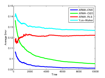
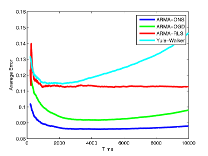
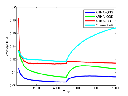
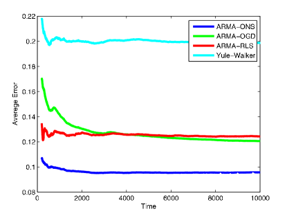
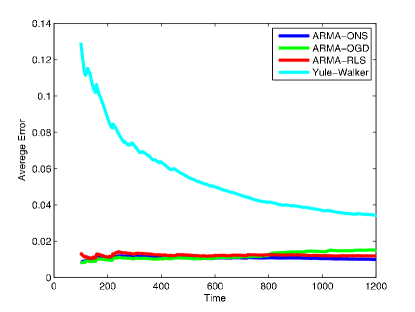
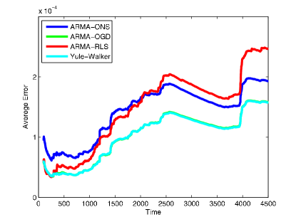
The following experiments demonstrate the prediction effectiveness of the proposed algorithms, under some different settings. We compare the performance to the ARMA-RLS algorithm, which was presented in [DSC06]. In a few words, the ARMA-RLS is a “proper learning” algorithm — it tries to mimic the underlying model. It estimates the noise terms using a recursive least squares based method, and satisfies a prediction using these estimations and the previous signals. The ARMA-RLS does not assume noise stationarity or ergodicity. We also benchmark the standard Yule-Walker estimation method333Yule-Walker estimation method is offline. We use it as an online prediction method by a simple adaptation — we let it predict the signal at time t𝑡t with the knowledge of the signal at times 1,,t11𝑡11,\ldots,t-1.. The results are displayed in the figures below. In all cases, the x𝑥x-axis is time (number of samples), and the y𝑦y-axis is the average squared loss.

5.1 Experiments with artificial data

In all experimental settings below we have averaged the results over 20 runs for stability. Also, we choose the order of our AR prediction to be m+k=10𝑚𝑘10m+k=10 in all settings.

Refer to caption
(a) Setting 1. Sanity check
Refer to caption
(b) Setting 2. Slowly changing coefficients
Refer to caption
(c) Setting 3. Abrupt change
Refer to caption
(d) Setting 4. Correlated noise
Figure 1: Experimental results for artificial data, all averaged over 20 runs.

Setting 1. We started with a simple sanity check using Gaussian noise. We generated a stationary ARMA process using the coefficient vectors α=[0.6,0.5,0.4,0.4,0.3]𝛼0.60.50.40.40.3\alpha=[0.6,-0.5,0.4,-0.4,0.3] and β=[0.3,0.2]𝛽0.30.2\beta=[0.3,-0.2], when the noise terms are uncorrelated and normally distributed as 𝒩(0,0.32)𝒩0superscript0.32\mathcal{N}(0,0.3^{2}). Note that since predicting the noise is impossible, a perfect predictor will suffer an average error rate of at least the variance of the noise — 0.09 in this setting. As can be seen in Figure 1(a) the ARMA-ONS algorithm outperforms the other online algorithms due to its lower regret in this setting of exp-concave loss functions, and quickly approaches the performance of the perfect predictor.

Setting 2. We generated the non-stationary ARMA process using the coefficient vectors β=[0.32,0.2]𝛽0.320.2\beta=[0.32,-0.2] and

α(t)𝛼𝑡\displaystyle\alpha(t) =\displaystyle= [0.4,0.5,0.4,0.4,0.1](t104)+[0.6,0.4,0.4,0.5,0.4](1t104),0.40.50.40.40.1𝑡superscript1040.60.40.40.50.41𝑡superscript104\displaystyle[-0.4,-0.5,0.4,0.4,0.1]*\Big{(}\frac{t}{10^{4}}\Big{)}+[0.6,-0.4,0.4,-0.5,0.4]*\Big{(}1-\frac{t}{10^{4}}\Big{)},

i.e., the coefficient vectors change slowly in time. The noise terms are uncorrelated and distributed uniformly on [0.5,0.5]0.50.5[-0.5,0.5] (denoted as Uni[0.5,0.5]𝑈𝑛𝑖0.50.5Uni[-0.5,0.5]). In this setting, a perfect predictor will suffer average error rate of at least 0.0833, due to the variance of the noise. The motivation behind this setting is to demonstrate the effectiveness of the online algorithms in the non-stationary case, in which the coefficients change in time. This is especially important when dealing with real data time series, since the stationarity assumption is rather strict. In Figure 1(b) we can see the clear advantage of our online algorithms. Here again, ARMA-ONS is superior to the other algorithms, despite it being less adaptive — as the theoretical bounds predict; see [HS09] for discussion of adaptivity of OGD vs. ONS.

Setting 3. Here we consider the non-stationary ARMA process that is generated using two different sets of coefficient vectors. The first set is α=[0.6,0.5,0.4,0.4,0.3]𝛼0.60.50.40.40.3\alpha=[0.6,-0.5,0.4,-0.4,0.3] and β=[0.3,0.2]𝛽0.30.2\beta=[0.3,-0.2], and it is used for generating the signal at the first half of the iterations. The second set is α=[0.4,0.5,0.4,0.4,0.1]𝛼0.40.50.40.40.1\alpha=[-0.4,-0.5,0.4,0.4,0.1] and β=[0.3,0.2]𝛽0.30.2\beta=[-0.3,0.2], and it is used for generating the signal at the second half of the iterations. The noise terms are uncorrelated and distributed Uni[0.5,0.5]𝑈𝑛𝑖0.50.5Uni[-0.5,0.5]. In Figure 1(c) we demonstrate the effectiveness of online algorithms in a scenario when the coefficients abruptly change. Here again, a perfect predictor will suffer average error rate of at least 0.0833, due to the variance of the noise.

Setting 4. Consider an ARMA process that is generated using the coefficient vectors α=[0.11,0.5]𝛼0.110.5\alpha=[0.11,-0.5] and β=[0.41,0.39,0.685,0.1]𝛽0.410.390.6850.1\beta=[0.41,-0.39,-0.685,0.1]. Each noise term is distributed normally, with expectation that is the value of the previous noise term, and variance 0.32superscript0.320.3^{2}. I.e., the noise terms are positively correlated. In Figure 1(d) one can clearly see the robustness of online algorithms to correlated noise. Note that despite the correlativity introduced in this setting, ARMA-ONS achieves an average error rate that converges approximately to the variance of the noise — 0.09.

5.2 Experiments with real data

In this section we provide some preliminary results on real data time series, and show that for such data as well, our online learning approach is reasonably effective compared to existing approaches. For robustness, we consider time series from different fields.
Refer to caption
(a) Monthly average temperature
Refer to caption
(b) S&P 500 daily returns
Figure 2: Experimental results for real data.

The first time series is taken from the field of weather research. Each data point in this time series is the monthly average temperature of the sea surface, measured at a specific point. The data is taken from the Global Climate Observing System (GCOS) website. Since we are dealing with a weather related time series, and considering the monthly average temperature, it is rather reasonable that the time series follows a certain pattern. As can be seen in Figure 2(a), this pattern can be well learned using the ARMA model by all four algorithms. However, the results clearly indicate the superiority of online algorithms.

The second time series is taken from the field of finance. Each data point in this time series is the daily return of the S&P 500 index. The data is taken from Yahoo! Finance. The results in Figure 2(b) indicate that the ARMA model is probably not a good model for predicting the returns of the S&P 500 index. A possible reason is that the ARMA model is not rich enough, i.e., knowing the history of returns is not sufficient for satisfying a good prediction. The fact that offline familiar methods also fail here, strengthens this claim. See Section 6 for further discussion about fitting a time series model for financial data.

6 Conclusion and discussion

In this paper we developed a new approach for time series analysis — an online learning approach. Our main result in this paper is that one can predict time series as well as the best ARMA model, regardless of the loss function considered, under weak assumptions on the noise terms — zero mean distribution. This result is strengthened in light of the fact that the noise terms in the underlying model are unknown to us at any stage. We overcome this difficulty by using improper learning techniques. Additionally, we present an analytical extension of our approach to adversarially generated noise terms. The main powerful properties of the online approach, as pointed out in our work, are generality, simplicity and efficiency, in comparison to existing methods.

There are three issues that remain for further research. First, in our analysis we assume that i=1q|βi|<1εsuperscriptsubscript𝑖1𝑞subscript𝛽𝑖1𝜀\sum_{i=1}^{q}|\beta_{i}|<1-\varepsilon for some ε>0𝜀0\varepsilon>0, which seems to limit the freedom of the β𝛽\beta coefficients. This assumption appears sometimes in the literature (e.g. in GARCH models) and is a sufficient condition for the MA component to be causally invertible, yet not necessary. In our case, we believe that this assumption follows from our proof techniques and the results would still hold for any β𝛽\beta coefficients. Second, in Section 4 we present results in which the total loss suffered by our algorithms is compared to the expected loss suffered by ARMA prediction with the coefficient vectors that have generated the signal. Whereas competing against the best ARMA prediction under adversarial noise is impossible because of identifiability issues, it would be interesting to study intermediate setups such as correlated or adversarial noise to some extent. Third, the ARMA model is not compatible for any time series, as can be seen in Section 5.2, when a finance related time series is considered. However, [Eng82] showed that some finance related time series can be well predicted using the ARCH model and its expansions. Therefore, it would be interesting to generalize our work to other time series models, such as ARCH and ARIMA.

References

  • [BD09] P. Brockwell and R. Davis. Time Series: Theory and Methods. Springer, 2 edition, 2009.
  • [BJR94] G. Box, G. Jenkins, and G. Reinsel. Time Series Analysis: Forecasting and Control. Prentice-Hall, 3 edition, 1994.
  • [CBL06] N. Cesa-Bianchi and G. Lugosi. Prediction, learning, and games. Cambridge University Press, 2006.
  • [DES89] E. Damsleth and A. H. El-Shaarawi. ARMA models with double-exponentially distributed noise. Journal of the Royal Statistical Society. Series B, 51(1):61–69, 1989.
  • [DSC06] F. Ding, Y. Shi, and T. Chen. Performance analysis of estimation algorithms of nonstationary ARMA processes. IEEE Transactions on Signal Processing, 33(3):1041–1053, 2006.
  • [Eng82] R.F. Engle. Autoregressive conditional heteroscedasticity with estimates of the variance of united kingdom inflation. Econometrica, 50:987–1007, 1982.
  • [HAK07] E. Hazan, A. Agarwal, and S. Kale. Logarithmic regret algorithms for online convex optimization. Machine Learning, 69(2-3):169–192, 2007.
  • [Ham94] J. Hamilton. Time Series Analysis. Princeton Univ. Press, 1994.
  • [HS09] E. Hazan and C. Seshadhri. Efficient learning algorithms for changing environments. In ICML, page 50, 2009.
  • [SS05] R. Shumway and D. Stoffer. Time Series Analysis and Its Applications. Springer, 2005.
  • [Tho94] D. Thomson. Jackknifing multiple-window spectra. In ICASSP, volume 6, pages VI/73 – VI/76, April 1994.
  • [TWVB00] M. Tiku, W. K. Wong, D. Vaughan, and G. Bian. Time series models in non-normal situations: Symmetric innovations. Journal of Time Series Analysis, 21(5):571–596, 2000.
  • [Zin03] M. Zinkevich. Online convex programming and generalized infinitesimal gradient ascent. In ICML, pages 928–936, 2003.