Thermostated Hamiltonian dynamics with log-oscillators

Abstract

With this work we present two new methods for the generation of thermostated, manifestly Hamiltonian dynamics and provide corresponding illustrations. The basis for this new class of thermostats are the peculiar thermodynamics as exhibited by logarithmic oscillators. These two schemes are best suited when applied to systems with a small number of degrees of freedom.

I Introduction

Back in 1984 Nosé put forward a method for the generation of equations of motion that sample the canonical ensemble Nose84JCP81 . The method is based on the Nosé Hamiltonian, reading:

$$H=\sum_{i}\frac{p_{i}^{2}}{2m_{i}X^{2}}+V(\mathbf{x})+\frac{P^{2}}{2M}+k_{B}T\ln{X}$$ (1)

where a log-oscillator with Hamiltonian ${P^{2}}/{2M}+k_{B}T\ln{X}$, is non-linearly coupled to a “virtual” system $(\mathbf{x},\mathbf{p})$. The thermostated dynamics of the “real” system are obtained after a time-rescaling and the application of a non-canonical transformation. The method was later further developed by Hoover Hoover85PRA31 , and is currently widely used and known as the Nosé-Hoover thermostat.

In this paper we unveil those special thermodynamic properties of log-oscillators which provide them with the power to act as thermostats and, based on them, show two more ways in which log-oscillators can be employed to generate thermostated dynamics. At variance with the method of Nosé, these methods are genuinely Hamiltonian, in the sense that the thermostated dynamics are obtained directly from Hamilton’s equations of motion, with no need to perform a time rescaling nor the use of non-canonical transformations Klages ; Kusnezov . Consequently these methods not only constitute a numerical means but, as well, can even be implemented in situ with real experiments aimed at thermostating a physical system. The first of the two methods has been reported recently with a letter, see in Ref. 5. Its feasibility has been further discussed with a short account in Ref. 6, providing there the response which dispels a criticism raised by Hoover and co-workers Melendez13PRL110 .

It is important to stress that, just like the Nosé-Hoover method, these methods only work provided the overall dynamics are ergodic, which might present a problem, – especially when applied to small systems. In the case of Nosé-Hoover thermostating one possible solution was offered by Martyna et al. Martyna92JCP97 , who proposed the use of chains of Nosé- Hoover thermostats. Our first method, at least in the implementation we have explored [that is considering a system of particles which interact with each other and with a log-oscillator via short range hard core repulsion, see 21 below] seemingly is immune in reference to this ergodicity issue Campisi12PRL108 ; Campisi12UNPUB1 ; Campisi12UNPUB2 . Regarding our second method, see 29 below, the absence of ergodicity may present an issue; this second method, however, is sufficiently flexible as to overcome this challenge.

II Helmholtz Theorem

The fact that logarithmic oscillators have a thermostating power is a consequence of their peculiar thermodynamic properties. In this section we shall clarify in what sense it is meaningful to talk about the thermodynamics of mechanical systems that have only one or few degrees of freedom, – as it is the case of logarithmic oscillators, and demonstrate how to calculate their thermodynamic properties.

Our starting point is the salient equation of thermodynamics:

$$\delta Q/T=\text{exact differential}=dS$$ (2)

also known as the heat theorem GallavottiBook . As early as 1884, Helmholtz proved that this mathematical structure of thermodynamics is inherent to the classical Hamiltonian dynamics of systems having only one single trajectory for each energy, which he called monocyclic systems HelmholtzINBOOK . Arguably, this seldom appreciated and rarely known fact was one of the cornerstones on which ergodic theory (which generalizes Helmholtz monociclicity) and statistical mechanics were later built up by Boltzmann and others GallavottiBook ; Campisi05SHPMP36 ; Campisi10AJP78 ; Hertz10AP338a .

The Helmholtz theorem goes as follows: Consider a classical particle in a confining potential $\varphi(X;\lambda)$, where $\lambda$ is an external parameter. To each couple ($E,\lambda$) of values of the energy and the external parameter is associated one closed trajectory in the system phase space. For each trajectory one can calculate the average quantities:

$$k_{B}T(E,\lambda) :=\left\langle\frac{P^{2}}{M}\right\rangle_{E,\lambda}$$ (3)

$$F(E,\lambda) :=-\left\langle\frac{\partial\varphi}{\partial\lambda}\right\rangle_{E,\lambda}$$ (4)

where $P,M$ are the particle momentum and mass respectively, and $\langle\cdot\rangle_{E,\lambda}$ denotes time average over the trajectory specified by $(E,\lambda)$. Noticing that $F(E,\lambda)$ is the average force that the particle exerts against the external agent, keeping the parameter $\lambda$ at a fixed value, one realizes that

$$\delta Q=dE+F(E,\lambda)d\lambda$$ (5)

represents the heat differential. The Helmholtz theorem states that $1/T(E,\lambda)$ is an integrating factor for $\delta Q$,

$$\frac{dE+F(E,\lambda)d\lambda}{T(E,\lambda)}=\text{exact differential}=dS$$ (6)

and that

$$S(E,\lambda)=k_{B}\ln\Phi(E,\lambda)$$ (7)

where

$$\Phi(E,\lambda) =\left[2\int_{X_{-}(E,\lambda)}^{X_{+}(E,\lambda)}\sqrt{2M(E-\varphi(X;\lambda))}dX/h\right]$$

$$=\int dXdP\,\theta[E-H(X,P)]\,.$$ (8)

Here, ${X_{\pm}(E,\lambda)}$ are the turning points of the trajectory, $h$ is a constant with the units of an action, and $\theta(x)$ denotes Heaviside step function. Accordingly it is meaningful to call $T(E,\lambda)$ the temperature of the particle and $S(E,\lambda)$ its entropy. $S(E,\lambda)$ in 7 is also known as the Hertz entropy Hertz10AP338a .

Once the function $S(E,\lambda)$ is known, one can then quickly calculate $T(E,\lambda)$ and $F(E,\lambda)$ in accordance to 6, as:

$$T =\left(\frac{\partial S}{\partial E}\right)^{-1}$$ (9)

$$F =\frac{\partial S}{\partial\lambda}\left(\frac{\partial S}{\partial E}\right)^{-1}$$ (10)

and so obtain the thermodynamics of the system: equation of state, specific heat, etc..

Following this scheme, in the next section, we will proceed to derive the thermodynamics of log-oscillators and highlight the peculiar properties that provide them with thermostating power.

III The peculiar thermodynamics of a log-oscillator

III.1 The heat capacity is infinite

Let us consider a log-oscillator with Hamiltonian:

$$H_{\text{log}}(X,P)=\frac{P^{2}}{2M}+k_{B}T\ln\frac{|X|}{b}\,,$$ (11)

where $M$ is the mass and $b$ some positive constant with the dimension of length. Figure 1 depicts some trajectories in phase space of different energies. Solving the equation $H_{\text{log}}(X,P)=E$ for $X$, one sees that the trajectories are given by the equations:

$$X=\pm\,b\,e^{E/k_{B}T}e^{-P^{2}/2Mk_{B}T}\;.$$ (12)

That is the trajectories possess a Gaussian shape. Note that, accordingly, the maximal excursion grows exponentially with $E/k_{B}T$: $X_{max}=b\,e^{E/k_{B}T}$.

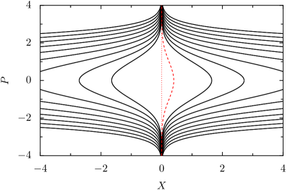
Figure 1: (Color online) Black solid lines: Phase space trajectories of a log-oscillator at energies $E=1/2,1,3/2,\dots 9/2$, inner curves have lower energies. Red dashed line: the momentum distribution function, 17. Here $M=1$, $k_{B}T=1$.

A straightforward calculation gives:

$$\Phi_{\text{log}}(E)=\int dXdP\,\theta[E-H_{\text{log}}(X,P)]=2b\sqrt{2\pi Mk_{B}T}e^{E/k_{B}T}\,.$$ (13)

Here, and in what follows we have set for convenience $h=1$. Accordingly, the entropy, 7, reads:

$$S(E) =\frac{E}{T}+k_{B}\ln[2b\sqrt{2\pi Mk_{B}T}].$$ (14)

Using the Helmholtz theorem, we get:

$$\langle P^{2}/M\rangle_{E}=(\partial S/\partial E)^{-1}=k_{B}T.$$ (15)

This expresses the major feature of the thermodynamics of a log-oscillator: all its trajectories inherit one and the same absolute temperature, which is given by $T$, where $T$ is the strength of the logarithmic potential. This fact is very peculiar: Consider for example the 1D harmonic oscillator, in this case $k_{B}T(E)=E$, namely the higher the energy, the higher the temperature. Similarly this is the case for a particle in a 1D box, where $k_{B}T(E)=E/2$.

It therefore follows that the log-oscillator possesses a spectacular property: it has an infinite heat capacity; i.e.,

$$C(E) =(\partial T/\partial E)^{-1}=\infty$$ (16)

thus, it mimics a bath composed of an infinite collection of harmonic oscillators Chaos2005 , or one with an infinite number of particles in a box.

III.2 Log-oscillators sample the Maxwell distribution

Yet another peculiar feature of the log-oscillator is that the probability density $f(P)$ to find it with momentum $P$, is given by the Maxwell distribution at temperature $T$:

$$f(P)=(2\pi Mk_{B}T)^{-1/2}e^{-P^{2}/2Mk_{B}T}\;.$$ (17)

This holds independent of its energy $E$. To see this, consider the trajectory of the log-oscillator of some energy $E$. The probability to find the system at $X,P$, is given by the microcanonical distribution:

$$\rho(X,P)=\delta[E-H_{\text{log}}(X,P)]/\Omega_{\text{log}}(E)$$ (18)

where $\delta(x)$ denotes Dirac’s delta function, and

$$\Omega_{\text{log}}(E) =\int dXdP\,\delta[E-H_{\text{log}}(X,P)]$$

$$=\frac{\partial\Phi_{\text{log}}(E)}{\partial E}=2b\sqrt{2\pi M/k_{B}T}\,e^{E/k_{B}T}\,.$$ (19)

Therefore, the probability to find the log-oscillator at momentum $P$, is obtained by the marginal distribution:

$$f(P) =\int dX\rho(X,P)=\int dX\delta[E-H_{\text{log}}(X,P)]/\Omega_{\text{log}}(E)$$

$$=\frac{1}{\Omega_{\text{log}}(E)}\frac{\partial}{\partial E}\int dX\theta[E-P^{2}/2M-k_{B}T\ln\frac{|X|}{b}]$$

$$=\frac{2}{\Omega_{\text{log}}(E)}\frac{\partial}{\partial E}\int_{0}^{b\exp[(E-P^{2}/2M)k_{B}T]}dX$$

$$=\frac{2}{\Omega_{\text{log}}(E)}\frac{\partial}{\partial E}be^{(E-P^{2}/2M)/k_{B}T}=\frac{e^{-P^{2}/2Mk_{B}T}}{\sqrt{2\pi Mk_{B}T}}$$ (20)

where we have used $\delta(y)=d\theta(y)/dy$.

From 17 it is immediate to obtain that $T(E)=\langle P^{2}\rangle_{E}/Mk_{B}=T$, in accordance with 15.

The red dashed curve in Fig. 1 illustrates 17. When projecting the microcanonical distribution of the log-oscillator onto the $P$ axis, the Maxwell distribution is obtained, regardless of the energy.

IV Method I

The central feature of a thermal bath is that its heat capacity is infinite, hence, in this sense a single log-oscillator does indeed act like a thermal bath. Based on this observation it is reasonable to expect that when a system interacts weakly with a log-oscillator, the latter should induce thermostated dynamics at temperature $T$ in the system.

That this is indeed the case can be seen formally in the following manner Campisi12PRL108 . Consider the total Hamiltonian:

$$H(\mathbf{x},\mathbf{p},X,P)=H_{S}(\mathbf{x},\mathbf{p})+H_{\text{log}}(X,P)+h(\mathbf{x},X)$$ (21)

where

$$H_{S}(\mathbf{x},\mathbf{p})=\mathbf{p}^{2}/2m+U(\mathbf{x})$$ (22)

is the system Hamiltonian, and $h(\mathbf{x},X)$ is a weak interaction term that couples the system to the log-oscillator. Under the assumption that the total dynamics are ergodic, the probability density function $p(\mathbf{x},\mathbf{p})$ for finding the system at $(\mathbf{x},\mathbf{p})$ reads Khinchin49Book :

$$p(\mathbf{x},\mathbf{p})=\frac{\Omega_{\text{log}}[E_{\text{tot}}-H_{S}(\mathbf{x},\mathbf{p})]}{\Omega(E_{\text{tot}})}$$ (23)

where $E_{\text{tot}}$ is the total energy of the compound system and

$$\Omega(E_{\text{tot}})=\int\mathrm{d}{X}\mathrm{d}{P}\mathrm{d}\mathbf{x}\mathrm{d}\mathbf{p}\,\delta[E_{\text{tot}}-H(\mathbf{x},\mathbf{p},X,P)]$$ (24)

is the density of states of the compound system. Note that the shape of the distribution $p(\mathbf{x},\mathbf{p})$ is given by the numerator, whereas the denominator only represents a normalization factor. Thus, from the fact that the density of states of a log-oscillator is exponential in ${E/k_{B}T}$, see 19, it immediately follows that:

$$p(\mathbf{x},\mathbf{p})=\frac{e^{-H_{S}(\mathbf{x},\mathbf{p})/k_{B}T}}{Z(T)}$$ (25)

where $Z(T)=\int d\mathbf{x}d\mathbf{p}\,e^{-H_{S}(\mathbf{x},\mathbf{p})/k_{B}T}$. Thus, the constant temperature equations of motion read:

$$\left\{\begin{array}[]{lll}\dot{\mathbf{x}}=\mathbf{p}/m,\\ \dot{\mathbf{p}}=-\partial_{\mathbf{x}}U(\mathbf{x})-\partial_{\mathbf{x}}h(\mathbf{x},X)\\ \dot{X}=P/M\\ \dot{P}=-k_{B}T/X-\partial_{X}h(\mathbf{x},X)\end{array}\right.$$

where $\partial_{\mathbf{x}}$ denotes the gradient operator in the $\mathbf{x}$ space and $\partial_{X}$ is a short notation for $\partial/\partial X$. Note that for $h=0$, i.e., in absence of interaction, the system undergoes constant energy dynamics.

Illustration

Ref. 5 illustrates the numerical implementation of this method for small systems composed of few particles contained in a box and interacting through a repulsive hard core potential

$$V_{LJ}(q)=\left\{\begin{array}[]{ll}0\,,&|q|>2^{1/6}\sigma\\ 4\varepsilon\left[\left(\frac{\sigma}{q}\right)^{12}-\left(\frac{\sigma}{q}\right)^{6}\right]+\varepsilon\,,&|q|<2^{1/6}\sigma\end{array}\right.\,,$$ (26)

The main limitation of this method comes from the fact that, in practical realizations, the logarithmic potential needs to be truncated at low values of $X$, for example by substituting it with:

$$\varphi_{b}(X)=\frac{k_{B}T}{2}\ln\frac{X^{2}+b^{2}}{b^{2}}\,.$$ (27)

This truncation results in a deviation of the single particle velocity distribution from the target Maxwell distribution. This deviation becomes more and more pronounced as the number of particles in the system increases, see Fig. 3 of Ref. 5, and can be compensated by rising the system energy as $E\sim fk_{B}T/2$, where $f$ is the number of degrees of freedom of the system. This energy rising, however, is accompanied by an exponential increase of the corresponding length and time scales involved in the dynamics which go as $e^{E/k_{B}T}\sim e^{f/2}$, thus limiting the applicability of the method to systems with a small number of degrees of freedom.

A prominent novel aspect of this method when compared to the other existing methods discussed in the literature is that it can be implemented not only with computer simulations but also in analogue simulations, provided one is able to implement the Hamiltonian in 21 in a real experiment Campisi12PRL108 . Reference 6 discusses such an experimental feasibility of this method using cold atoms and laser fields.

Figure 2 illustrates this method for a system composed of either one particle or two particles in a one-dimensional box performing short range, hard core collisions, 26, with the truncated log-oscillator in 27. It reports the probability $\rho(E_{S})$ to find the particle at energy $E_{S}$ during a long simulation run. A symplectic integrator was used to produce the trajectory of the total system and the initial condition was sampled randomly from the shell $E_{\text{tot}}=5k_{B}T$. The numerically computed probability (relative frequency) $\rho(E_{S})$ is compared to the expected Gibbs distribution calculated from 25 according to the standard rules of probability theory as

$$\rho(E_{S})=\frac{e^{-E_{S}/T}\Omega_{S}(E_{S})}{Z(T)}=\frac{e^{-E_{S}/T}\Omega_{S}(E_{S})}{\int_{0}^{\infty}e^{-E_{S}/T}\Omega_{S}(E_{S})dE_{S}}\,,$$ (28)

where $\Omega_{S}(E_{S})$ is the density of states of the system. In calculating it we neglect the contribution coming from the short range interaction, thus obtaining $\Omega_{S}(E_{S})\propto E_{S}^{n/2-1}$, with $n=1,2$ being the number of particles in the system. For $n=1$ this yields $\Omega_{S}(E_{S})\propto E_{S}^{-1/2}$ while for $n=2$ we find that $\Omega_{S}(E_{S})$ is a constant. The agreement between theory and simulations is excellent. Further details and discussion can be found in Refs. 5 and 10.

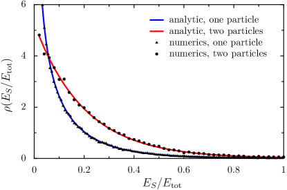
Figure 2: (Color online) Illustration of Method I. Normalized probability density function of energy for a system of $n$ particles in a 1D box performing short ranged collisions, 26, with a truncated log-oscillator, 27, of strength $k_{B}T=15\varepsilon$. The total simulation energy is $E_{\text{tot}}=5k_{B}T$, the box length is $L=10e^{E_{\text{tot}}/k_{B}T}\sigma\simeq 1484\sigma$ and the log-oscillator cutoff length was set to $b=\sigma$. Black triangles: numerical simulation with $n=1$. Black dots: numerical simulation with $n=2$. Blue line: Gibbs distribution at temperature $k_{B}T=15\varepsilon$ for $n=1$, as it follows from 28. Red line: Corresponding Gibbs distribution at temperature $k_{B}T=15\varepsilon$ for $n=2$ as it follows from 28. This Figure has been provided by Fei Zhan and is adapted here from our Ref. 10.

V Method II

An alternative method to produce thermostated dynamics is to couple the system to a free particle via a logarithmic interaction potential. More explicitly, the statement is that the extended Hamiltonian

$$H(\mathbf{x},\mathbf{p},X,P) =H_{S}(\mathbf{x},\mathbf{p})+P^{2}/2M+k_{B}T\ln\left(|g(\mathbf{x},\mathbf{p})-X|/b\right)$$ (29)

produces thermostated system dynamics, provided the (otherwise arbitrary) function $g(\mathbf{x},\mathbf{p})$ induces ergodic dynamics of the total system.

To demonstrate this, consider the probability $\rho(\mathbf{x},\mathbf{p},X,P)$ to find the total system at $(\mathbf{x},\mathbf{p},X,P)$. Thanks to the ergodic assumption, this is given by the microcanonical distribution

$$\rho(\mathbf{x},\mathbf{p},X,P)=\delta[E_{\text{tot}}-H(\mathbf{x},\mathbf{p},X,P)]/\Omega(E_{\text{tot}})\,,$$ (30)

hence:

$$p(\mathbf{x},\mathbf{p})=\frac{\int dXdP\delta[E_{\text{tot}}-H_{S}-P^{2}/2M-T\ln(|g-X|/b)]}{\Omega(E_{\text{tot}})}$$ (31)

Making the change of variable $X^{\prime}=X-g(\mathbf{x},\mathbf{p})$, one obtains, irrespective of $g(\mathbf{x},\mathbf{p})$

$$p(\mathbf{x},\mathbf{p})=\frac{\int dX^{\prime}dP\delta[E_{\text{tot}}-H_{S}-P^{2}/2M-k_{B}T\ln(|X^{\prime}|/b)]}{\Omega(E_{\text{tot}})}$$ (32)

Note that the numerator is the log-oscillator density of states $\Omega_{\text{log}}$ taken at $E_{\text{tot}}-H_{S}$. Therefore, just as with Method I:

$$p(\mathbf{x},\mathbf{p})=\frac{\Omega_{\text{log}}[E_{\text{tot}}-H_{S}(\mathbf{x},\mathbf{p})]}{\Omega(E_{\text{tot}})}=\frac{e^{-H_{S}(\mathbf{x},\mathbf{p})/k_{B}T}}{Z(T)}.$$ (33)

The constant temperature equations of motion of this second method read:

$$\left\{\begin{array}[]{lll}\dot{\mathbf{x}}=\mathbf{p}/m+k_{B}T[g(\mathbf{x},\mathbf{p})-X]^{-1}\partial_{\mathbf{p}}g(\mathbf{x},\mathbf{p})\\ \dot{\mathbf{p}}=-\partial_{\mathbf{x}}U(\mathbf{x},\mathbf{p})-k_{B}T[g(\mathbf{x},\mathbf{p})-X]^{-1}\partial_{\mathbf{x}}g(\mathbf{x},\mathbf{p})\\ \dot{X}=P/M\\ \dot{P}=k_{B}T[g(\mathbf{x},\mathbf{p})-X]^{-1}\end{array}\right.$$

note that for $T=0$ the system undergoes constant energy dynamics.

It is important to repeat that thermostated system dynamics are only reached if the global dynamics are ergodic. As illustrated below, this requirement is however not too restrictive, because we have the freedom to chose the function $g(\mathbf{x},\mathbf{p})$.

Illustration

To illustrate the method we considered a quartic oscillator:

$$H_{S}=p^{2}/2m+kx^{4}/4$$ (34)

We simulated the compound system dynamics using a symplectic integrator with a time step $\Delta t=10^{-2}b\sqrt{M/k_{B}T}$ for a total simulation time $\mathcal{T}=1.287\times 10^{9}\Delta t$ time steps. In our simulations we set $k_{B}T,b$ and $M$ as units of energy, length and mass, respectively. We took $(x_{0},X_{0},p_{0},P_{0})=(2,-1,1,-1)$ as the initial condition, $k=k_{B}Tb^{-4}$, and $m=M$. We computed the probability distribution function $\rho(E_{S})$ to find the system at energy $E_{S}$, and compared it with the target Gibbs distribution, 28. The latter reads

$$\rho(E_{S})=\frac{e^{-E_{S}/k_{B}T}E_{S}^{-1/4}}{\int_{0}^{\infty}\mathrm{d}E_{S}e^{-E_{S}/k_{B}T}E_{S}^{-1/4}}$$ (35)

where the factor $E_{S}^{-1/4}$ stems from the density of states of the quartic oscillator: $\int\mathrm{d}x\mathrm{d}p\delta[E_{S}-p^{2}/2m+kx^{4}/4]\propto E_{S}^{-1/4}$. We further computed the probability distribution function to find the system with a velocity of modulus $v$, and compared it to the target Maxwell distribution, reading:

$$p(v)=\frac{e^{-mv^{2}/2k_{B}T}}{\int_{0}^{\infty}e^{-mv^{2}/2k_{B}T}}$$ (36)

Following Ref. 5, the numerical evaluation of $\rho(E_{S})$ proceeded by recording the value of $E_{S}$, once every 100 time steps. We divided the energy interval $[0,E_{tot}]$ in 50 bins, and counted how many times $E_{S}$ was within each bin, so as to construct a histogram, which, after normalization gives an approximation to the actual $\rho(E_{S})$. A similar procedure was followed for the calculation of $p(v)$.

To begin with we chose $g(x,p)=x$. Notwithstanding the long integration time, the method fails to converge to the desired target distributions, see Fig. 3, panel a). This means that with the choice of $g(x,p)=x$, the overall dynamics is not sufficiently ergodic to make the system sample the canonical ensemble.

The ergodicity of the overall dynamics can be improved by choosing a different form for the function $g(x,p)$. Panel b) of Fig. 3 reports the result of a dynamical simulation of the same system as in panel a), with the same time-step $\Delta t$ and simulation time, but with $g(x,p)=kx^{4}/4$, namely we chose $g(x,p)$ as the system potential energy. While we found a very good agreement between the computed energy probability distribution function and the Gibbs distribution, the agreement between the computed absolute velocity distribution and the target Maxwell distribution is still not very good. With $g(x,p)=\sin(kx^{4}/4)$, see in panel c) of Fig. 3, reasonably good agreement between simulation and Maxwell distributions was achieved, while the agreement between the energy distribution and the Gibbs distribution is excellent. Excellent agreement is achieved with longer simulation times, see in panel d) of Fig. 3.

Figure 3: Illustration of Method II. Each panel reports the analytically and numerically computed probability distribution for system energy $E_{S}$ (rescaled by the total fixed energy $E_{\rm{tot}}$) and system speed $v$ (rescaled by the maximal speed $v_{\rm{max}}=\sqrt{2E_{\rm{tot}}/m}$), for various choices of $g(x,p)$. Panel d) has the same $g(x,p)$ as panel c), but for a longer simulation time.

VI Remarks

As emphasized above, ergodicity of the global dynamics constitutes the crucial prerequisite for the presented methods to work properly. Ergodicity suffices and no stronger condition, e.g., the system being mixing, Lebowitz73PT26 is necessary because all that is needed for the system to sample the Gibbs distribution is that the compound system samples the microcanonical distribution. It should also be mentioned that ergodicity is a sufficient but not necessary condition for the methods to work, namely in some cases the methods might work even if ergodicity does not hold.

In Method I, whether ergodicity holds depends on the specific choice of the interaction energy $h(\mathbf{x},X)$, which must be chosen in any case weak. In Ref. 5 $h(\mathbf{x},X)$ was chosen as a hard-core, short range repulsive interparticle potential, 26, and that was sufficient for achieving thermostating. In Method II, the ergodicity property depends on the choice of $g(\mathbf{x},\mathbf{p})$, which in turn fixes the interaction term $k_{B}T\ln|g(\mathbf{x},\mathbf{p})-X|$. It must be emphasized however that our analysis does neither show formally nor numerically that the total dynamics are indeed ergodic in the examples presented, but only that, loosely speaking, the system appears “ergodic enough” for the methods to work.

Note that in method II the interaction term $k_{B}T\ln|g(\mathbf{x},\mathbf{p})-X|$ gives rise to long-range forces. So at variance with the implementation of Method I in Ref. 5, where the system and the “bath” interacted sporadically through almost instantaneous collisions, in Method II they constantly influence each other, due to the long range force.

We have shown how different choices of $g(\mathbf{x},\mathbf{p})$ can result in different ergodic properties of Method II. An important subject for further studies would be to derive a set of criteria for appropriately choosing $g(\mathbf{x},\mathbf{p})$, given the properties of the system, as encoded in its Hamiltonian $H_{S}(\mathbf{x},\mathbf{p})$.

Besides choosing $h(\mathbf{x},X)$ or $g(\mathbf{x},\mathbf{p})$, the ergodicity of both methods can be improved also by substituting the log-oscillator with a multi-dimensional log-oscillator, which will add more degrees of freedom to the whole system, see in Appendix.

In implementing Method II, we have replaced the logarithmic potential with the same truncated potential, 27, used for Method I. Therefore, just as with Method I, this truncation can lead to deviations to the target Maxwell distribution when the number of particles in the system increases. An interesting line for future studies would then be to put forward implementations that avoid the truncation and treat the singularity by some other means, which might allow for applying the methods to large systems as well.

VII Conclusions

With this study we presented two Hamiltonian schemes which allow a system $H_{S}$ to sample a canonical Gibbs distribution. This being so, the method of thermostating is achieved here in a deterministic time-reversal invariant and symplectic manner. Both schemes rest upon the spectacular thermodynamic property of logarithmic oscillators of having an infinite heat capacity. Hence, in our methods a single log-oscillator substitutes an infinite heat bath coupled weakly to the system. With our Method I we couple the system weakly to a log-oscillator where the absolute temperature $T$ denotes the strength of the logarithmic potential. In Method II we consider a composite system of $H_{S}$ and a free particle which is coupled with a long range log-interaction of strength $T$ to the system of interest $H_{S}$. Note that Gibbs thermalization occurs here independent of the interaction-strength $T$, being either strong (large $T$) or weak (small $T$). A prominent property inherent to both schemes is that these are manifestly Hamiltonian Campisi12UNPUB1 . Also, at variance with the Nosé Hamiltonian, 1, our Hamilton functions possess standard (i.e. coordinate-independent) kinetic energy contributions. This fact in turn allows not only an implementation with numerical means but as well a physical realization. This advantage should be contrasted nevertheless with the limitation that both methods inherit from performing a truncation of the logarithmic potential as in 27, which, as thoroughly emphasized in our previous accounts Campisi12PRL108 ; Campisi13PRL110 , limits an efficient thermostating to systems with a small number of degrees of freedom. Notably, the investigation of such nano-scale systems is in the limelight of present day research activities Campisi11RMP83 ; Jarzynski11ARCMP2 ; Seifert08EPJB64 ; Bloch08RMP80 .

Appendix A Appendix. $f$ dimensional log-oscillators

Consider a $f$ dimensional log-oscillator:

$$H_{\text{log}}(\mathbf{X},\mathbf{P})=\frac{\mathbf{P}^{2}}{2M}+fk_{B}T\ln\frac{|\mathbf{X}|}{b}\,,$$ (37)

Where $\mathbf{X}=(X_{1},X_{2},...X_{f})$, $\mathbf{P}=(P_{1},P_{2},...P_{f})$. For the phase volume $\Phi_{\text{log}}(E)=\int_{H\leq E}d\mathbf{X}d\mathbf{P}$ one obtains:

$$\Phi_{\text{log}}(E)=\frac{\left(8\pi^{2}b^{2}Mk_{B}T/f\right)^{f/2}}{\Gamma(f+1)}e^{E/k_{B}T}$$ (38)

where $\Gamma$ denotes the Gamma function. Therefore, the density of states is exponential in $E/k_{B}T$; reading

$$\Omega_{\text{log}}(E)=\frac{\partial\Phi_{\text{log}}(E)}{\partial E}=\frac{\left(8\pi^{2}b^{2}Mk_{B}T/f\right)^{f/2}}{k_{B}T\,\Gamma(f+1)}e^{E/k_{B}T}\;.$$ (39)

Consequently, the methods presented above can also be implemented with an $f$ dimensional oscillators replacing the 1 dimensional oscillator: In this case Method I becomes:

$$\left\{\begin{array}[]{lll}\dot{\mathbf{x}}=\mathbf{p}/m,\\ \dot{\mathbf{p}}=-\partial_{\mathbf{x}}U(\mathbf{x})-\partial_{\mathbf{x}}h(\mathbf{x},X)\\ \dot{\mathbf{X}}={\mathbf{P}}/M\\ \dot{\mathbf{P}}=-[k_{B}T/\mathbf{X}^{2}]{\mathbf{X}}-\partial_{\mathbf{X}}h(\mathbf{x},X)\end{array}\right.$$

and Method II becomes

$$\left\{\begin{array}[]{l}\dot{\mathbf{x}}=\mathbf{p}/m+[k_{B}T/(\mathbf{g}-\mathbf{X})^{2}]\sum_{k}(g_{k}-X_{k})\partial_{\mathbf{p}}\,g_{k}\\ \dot{\mathbf{p}}=-\partial_{\mathbf{x}}U-[k_{B}T/(\mathbf{g}-\mathbf{X})^{2}]\sum_{k}(g_{k}-X_{k})\partial_{\mathbf{x}}\,g_{k}\\ \dot{\mathbf{X}}=\mathbf{P}/M\\ \dot{\mathbf{P}}=[k_{B}T/(\mathbf{g}-\mathbf{X})^{2}](\mathbf{g}-\mathbf{X})\end{array}\right.$$

where $\mathbf{g}$, a short notation for $\mathbf{g}(\mathbf{x},\mathbf{p})=(g_{1}(\mathbf{x},\mathbf{p}),\dots,g_{f}(\mathbf{x},\mathbf{p}))$, is an $f$-dimensional field.

References

- (1) Nosé, S. A Unified Formulation of the Constant Temperature Molecular Dynamics Methods. J. Chem. Phys. 1984, 81, 511.
- (2) Hoover, W. G. Canonical Dynamics: Equilibrium Phase-space Distributions. Phys. Rev. A 1985, 31, 1695.
- (3) Klages, R. Microscopic Chaos, Fractals and Transport in Noneq. Statistical Mechanics, Adv. Ser. Nonl. Dyn. 24 (World Scientific, Singapore, 2007), cf. Part II.
- (4) Kusnezov, D.; Bulgac, A.; Bauer, W. Canonical Ensembles from Chaos. Ann. Phys. (N.Y.) 1990 204, 155; see p. 160, below Eq. (12).
- (5) Campisi, M.; Zhan, F.; Talkner, P.; Hänggi, P. Logarithmic Oscillators: Ideal Hamiltonian Thermostats. Phys. Rev. Lett. 2012, 108, 250601.
- (6) Campisi, M.; Zhan, F.; Talkner, P.; Hänggi, P. Campisi et al. Reply. Phys. Rev. Lett. 2013, 110, 028902.
- (7) Meléndez, M.; Hoover, W. G.; Español, P. Comment on “Logarithmic Oscillators: Ideal Hamiltonian Thermostats”. Phys. Rev. Lett. 2013, 110, 028901.
- (8) Martyna, G. J.; Klein, M. L.; Tuckerman, M. Nosé–Hoover chains: The Canonical Ensemble via Continuous Dynamics. J. Chem. Phys. 1992, 97, 2635.
- (9) Campisi, M.; Zhan, F.; Talkner, P.; Hänggi, P. Reply to W. G. Hoover. arXiv:1204.4412 2012.
- (10) Campisi, M.; Zhan, F.; Talkner, P.; Hänggi, P. Reply to M. Meléndez and W. G. Hoover. arXiv:1207.1859 2012.
- (11) Gallavotti, G. Statistical Mechanics: a Short Treatise; Springer: Berlin, 1999.
- (12) Helmholtz, H. In: Wissenschaftliche Abhandlungen; Wiedemann, G., Ed.; Johann Ambrosius Barth: Leipzig, 1895; Vol. 3; pp 142–162, 163–178, 179–202.
- (13) Campisi, M. On the Mechanical Foundations of Thermodynamics: The Generalized Helmholtz Theorem. Stud. Hist. Phil. Mod. Phys. 2005, 36, 275–290.
- (14) Campisi, M.; Kobe, D. H. Derivation of the Boltzmann Principle. Am. J. Phys. 2010, 78, 608–615.
- (15) Hertz, P. Über die mechanischen Grundlagen der Thermodynamik. Ann. Phys. (Leipzig) 1910, 338, 225–274, 537–552.
- (16) Hänggi, P.; Ingold, G. L. Fundamental Aspects of Quantum Brownian Motion. Chaos 2005 15, 026105.
- (17) Khinchin, A. Mathematical foundations of statistical mechanics; Dover: New York, 1949.
- (18) Lebowitz, J. L.; Penrose, O. Modern Ergodic Theory. Physics Today 1973 26, 23-29.
- (19) Campisi, M.; Hänggi, P.; Talkner P. Colloquium: Quantum Fluctuation Relations: Foundations and Applications. Rev. Mod. Phys. 2011 83, 771–79; Rev. Mod. Phys. 2011 83, 1653.
- (20) Jarzynski, C. Equalities and Inequalities: Irreversibility and the Second Law of Thermodynamics at the Nanoscale. Annu. Rev. Condens. Matter Phys. 2011 2, 329–351.
- (21) Seifert U. Stochastic Thermodynamics, Fluctuation Theorems and Molecular Machines. Rep. Prog. Phys. 2012 75, 126001
- (22) Bloch, I; Dalibard, J.; Zwerger W. Many-body Physics with Ultracold Gases. Rev. Mod. Phys. 2008 80, 885.