Ferromagnetic to antiferromagnetic transition of one-dimensional spinor Bose gases with spin-orbit coupling

Abstract

We investigate the interacting two-component bosonic gases with spin-orbit (SO) coupling in one dimension. Through a gauge transformation, the effect of SO coupling is incorporated into a spin-dependent twisted boundary condition. We solve the SO coupled system analytically by using the BA method. Our result shows that the SO coupling can influence the eigenenergy in a periodical pattern. The interplay between interaction and SO coupling may induce the energy level crossings for the lowest energy spectrum, which leads to a transition from the ferromagnetic to antiferromagnetic state.

I Introduction

The experimental success in manipulating cold atoms in effective one-dimensional (1D) waveguides has deepened our understanding of the properties of the low-dimensional quantum gases Paredes ; Toshiya ; Cazalilla ; GuanXW . Meanwhile, studies of synthetic gauge field in cold atom systems have also made great progresses: pioneering experiments of NIST group have generated the effective magnetic fields, electric fields and spin-orbit (SO) coupling in ultracold Bose gases Y.-J. Lin . The SO-coupled Fermionic gases have also been realized recently Zhang ; Zwierlein . Intriguing phenomena in condensed matter physics, such as quantum spin Hall effect and topological insulators X. L. Qi ; M. Z. Hasan , where electrons play the elemental role in these physical systems, are revealed in the SO coupling systems. The realization of SO coupling in cold bosonic systems opens a completely new avenue for studying the physics of Abelian or non-Abelian gauge potentials beyond the traditional condensed matter physics.

Many theoretical researches have revealed interesting phenomena for SO coupled bosonic systems. For example, a single plane wave phase or a stripe phase in spin-1/2 Bose-Einstein condensates (BECs) with SO coupling has been predicted depending on the intraspecies interaction larger or smaller than that of interspecies C. Wang ; Ho . The collective modes W. Zheng , stability of BECs with SO coupling Ozawa ; BiaoWu , and the phases in the presence of harmonic traps and rotation Wu ; X.-Q. Xu ; J. Radi'c ; B. Ramachandhran ; S. Sinha ; ZFXu have also been studied. Most of these investigations restricted on mean-field approximation in the weakly interacting regime. However, mean-field theory fails in the strong interaction limit. In order to get a complete physical picture of SO coupled system, the exact solution for SO coupled cold atom system is highly desirable.

In this paper, we solve analytically the SO coupled spin-1/2 bosonic system in a ring trap by the Bethe-ansatz (BA) method. In this system, SO coupling affect the eigenenergy periodically. A pioneering research proposed to realize the spatially periodic Raman coupling for a two component Bose-Einstein condensates by using two intersecting laser beam, which provides a platform to investigate these system experimentally J. Higbie . The SO coupling brings new physics to Bosonic system, particularly in the strongly interacting regime. In the absence of SO coupling, the ground state of the spin-1/2 bosonic system is the ferromagnetic state by solving BA equations Y. Q. Li ; Guan Xiwen ; Yajiang Hao ; Fuchs . By adding the SO coupling, we find that the competition between the SO coupling and interaction produce energy level crossings for the lowest energy spectrum in the strongly interacting regime. The ground state of the system may change from a ferromagnetic state to an antiferromagnetic state.

The present paper is organized as follows. In Section II, we introduce the model and solve it by using BA method. By employing a rather general transformation, SO coupling effect could be transformed to the twisted boundary condition. The eigenenergy is got by solving the BA equtions and the energy level crossings are shown. In Section III, we study the BA equations in the strongly interacting regime and demonstrate that the antiferromagnetic state can be the ground state. A summary is given in Section IV.

II Model and solution

We consider a two-component bosonic gas confined in a 1D ring trap in the presence of SO coupling with the Hamiltonian given by $\hat{H}=\hat{H}_{0}+\hat{H}_{\text{int}}$ with

$$\hat{H}_{0}=\int dx\hat{\Psi}^{{\dagger}}\left(x\right)\left(-\frac{\hbar^{2}}{2m}\frac{\partial^{2}}{\partial x^{2}}-2i\alpha\sigma_{z}\frac{\partial}{\partial x}\right)\hat{\Psi}\left(x\right),$$ (1)

where $\hat{\Psi}^{{\dagger}}=(\hat{\Psi}_{\uparrow}^{{\dagger}},\hat{\Psi}_{\downarrow}^{{\dagger}})$ represents two internal states of bosonic atoms, $\alpha$ denotes the spin-orbit coupling strength and $\sigma_{z}$ is the Pauli matrix. Here, we consider a quasi-one-dimensional situation with the transverse motion tightly confined in its ground state. The ring trap enforces the periodic boundary condition $\hat{\Psi}_{\sigma}\left(x\right)=\hat{\Psi}_{\sigma}\left(x+L\right)$. The interaction term is generally represented as $\hat{H}_{\text{int}}=\int dx(g_{1}\hat{n}_{\uparrow}^{2}+g_{2}\hat{n}_{\downarrow}^{2}+2g_{12}\hat{n}_{\uparrow}\hat{n}_{\downarrow})$, where $g_{1,2}$ and $g_{12}$ denote the strengths of intraspecies and interspecies interaction, which are experimentally tunable. In this work, we shall focus on the case with spin-independent interaction, i.e., $g_{1}=g_{2}=g_{12}=c$, for which interaction term can be represented as $\hat{H}_{\text{int}}=c\int dx\hat{n}^{2}$ with $\hat{n}=\hat{n}_{\uparrow}+\hat{n}_{\downarrow}$. We shall set $\frac{\hbar^{2}}{2m}=1$ in the following text for convenience.

It is difficult to solve the Hamiltonian with spin and momentum coupled together. Using a rather general transformation Shun Uchino

$$\hat{\Psi}_{\sigma}\left(x\right)=\hat{\Phi}_{\sigma}\left(x\right)e^{-i\alpha x\sigma_{z}},$$ (2)

the Hamiltonian is rewritten as follows,

$$\hat{H}_{0}=-\sum_{\sigma}\int dx\hat{\Phi}_{\sigma}^{{\dagger}}\left(x\right)\frac{\partial^{2}}{\partial x^{2}}\hat{\Phi}_{\sigma}\left(x\right)-N\alpha^{2},$$ (3)

and the form of $\hat{H}_{\text{int}}=c\int dx\hat{n}^{2}$ is invariant with $\hat{n}=\hat{\Phi}^{{\dagger}}\hat{\Phi}$ and $\hat{\Phi}^{{\dagger}}=(\hat{\Phi}_{\uparrow}^{{\dagger}},\hat{\Phi}_{\downarrow}^{{\dagger}})$. The operator $\hat{\Phi}_{\sigma}\left(x\right)$ and $\hat{\Phi}_{\sigma}^{{\dagger}}\left(x^{\prime}\right)$ also satisfy commutation relation $[\hat{\Phi}_{\sigma}^{{\dagger}}\left(x\right),\hat{\Phi}_{\sigma^{\prime}}\left(x\right)]=\delta_{\sigma\sigma^{\prime}}\delta(x-x^{\prime})$. Meanwhile, the total momentum now is represented as $\hat{K}=\sum_{\sigma}\int dx\hat{\Phi}_{\sigma}^{{\dagger}}\left(x\right)\left(-i\frac{\partial}{\partial x}-\alpha\sigma_{z}\right)\hat{\Phi}_{\sigma}\left(x\right)$ which is spin-dependent. The Schrödinger equation is $\hat{H}|\Phi\rangle=E|\Phi\rangle$, where the wave function is given by

$$|\Phi\rangle=\sum_{\kappa}\int\phi_{\kappa}\left(x_{1}...x_{N}\right)\prod_{i=1...N}\hat{\Phi}_{\sigma_{i}}^{+}\left(x_{i}\right)dx_{i}\left|0\right\rangle,$$ (4)

here $\kappa$ denotes $\sigma_{1},\sigma_{2}...,\sigma_{N}$ corresponding to the spin index for different particles. By applying the wave function to the Schrödinger equation, we get

$$H\phi_{\kappa}\left(x_{1},...,x_{N}\right)=E\phi_{\kappa}\left(x_{1},...,x_{N}\right)$$ (5)

with

$$H=-\sum_{i=1}^{N}\frac{\partial^{2}}{\partial x_{i}^{2}}+2c\sum_{i<j}\delta\left(x_{i}-x_{j}\right)-\alpha^{2}N,$$ (6)

It is worth mentioning that SO effect is not omitting but transformed to the spin-dependent twisted boundary condition. Explicitly, the periodic boundary condition $\hat{\Psi}_{\sigma}\left(x+L\right)=\hat{\Psi}_{\sigma}\left(x\right)$ under the transformation Eq.(2) is changed to be

$$\hat{\Phi}_{\sigma}\left(x+L\right)=\hat{\Phi}_{\sigma}\left(x\right)e^{i\sigma_{z}\alpha L},$$ (7)

Correspondingly, the wave function now should satisfy

$$\phi_{\kappa}\left(x_{1},...x_{j}+L...,x_{N}\right)=e^{i\sigma_{j,z}\alpha L}\phi_{\kappa}\left(x_{1},...x_{j}...,x_{N}\right).$$ (8)

The model of two-component bosons described by Eq.(6) is analytically solvable by BA under periodic boundary condition Y. Q. Li . The eigenstates can be characterized by the total spin $S$ of the system which varies from $0$ to $N/2$. The ground state of interacting two-component bosons corresponds to the ferromagnetic state with $S=N/2$. Now the problem of solving one-dimensional interacting two-component bosonic gases with SO coupling is simplified as solving the integrable model of (6) under the twisted boundary condition of (8), for which we can still obtain exact solutions by the same method as originally developed in B. S. Shastry . The system is solvable by the same Bethe-type wavefunction as below

$$\phi_{\kappa}\left(x_{1}...x_{N}\right) = \sum_{P,Q}\theta\left(x_{q_{N}}-x_{q_{N-1}}\right)...\theta\left(x_{q_{2}}-x_{q_{1}}\right)$$ (9)

$$\times A\left(Q,P\right)e^{i\sum_{j}k_{p_{j}}x_{q_{j}}},$$

where $Q=\{q_{1},q_{2},...,q_{N}\}$ and $P=\{p_{1},p_{2},...,p_{N}\}$ denote permutations of $1,...,N$. $\theta\left(x_{2}-x_{1}\right)$ is the step function and $\{k_{j}\}$ represent quasimomenta with $j=1,...,N$. $A\left(Q,P\right)$ are coefficients to be determined, which should fulfill the following relations

$$A\left(Q;...i,j...\right)=Y_{ji}^{ab}A\left(Q;...j,i...\right),$$ (10)

where $Y_{jl}^{ab}=\frac{\left(k_{j}-k_{l}\right)P_{q_{a}q_{b}}-ic}{k_{j}-k_{l}+ic}$ with $P_{q_{a},q_{b}}$ permutating $q_{a}$, $q_{b}$ in $A\left(...q_{a},q_{b}...,P\right)$. The scattering matrix remains the same as in the model with periodic boundary conditions. For eigenstate with total spin $S=\frac{1}{2}\left(N-2M\right)$ $(0\leq M\leq N/2)$ under the twisted boundary condition (8), we obtain the following BA equations

$$e^{i\left(k_{j}-\alpha\right)L}=-\prod_{l=1}^{N}\frac{k_{j}-k_{l}+ic}{k_{j}-k_{l}-ic}\prod_{\beta=1}^{M}\frac{k_{j}-\lambda_{\beta}-ic^{\prime}}{k_{j}-\lambda_{\beta}+ic^{\prime}},$$ (11)

$$\prod_{j=1}^{N}\frac{\lambda_{\zeta}-k_{j}-ic^{\prime}}{\lambda_{\zeta}-k_{j}+ic^{\prime}}=-e^{i2\alpha L}\prod_{\beta=1}^{M}\frac{\lambda_{\zeta}-\lambda_{\beta}-ic}{\lambda_{\zeta}-\lambda_{\beta}+ic},$$ (12)

where $c^{\prime}=c/2$ and $\{\lambda_{\beta}\}$ denote the spin rapidities. From the above BA equations Eq.(11) and Eq.(12), one can observe that the quasimomenta periodically depend on $\alpha$. So we let $\alpha=\alpha_{0}+\frac{2\pi n}{L}$ with $\alpha_{0}\in\left[0,\frac{2\pi}{L}\right]$ and $n$ being integer. In fact, we need only consider $\alpha_{0}\in\left[0,\frac{\pi}{L}\right]$. The quasimomentum for $\alpha_{0}\in\left[\frac{\pi}{L},\frac{2\pi}{L}\right]$ can be deduced from $\alpha_{0}\in\left[0,\frac{\pi}{L}\right]$ by two steps: first by taking $-\alpha_{0}\in\left[-\frac{\pi}{L},0\right]$ with solution $-k_{j}$ and $-\lambda_{\zeta}$, second by shifting $\alpha_{0}$ to $-\alpha_{0}+\frac{2\pi}{L}\in\left[\frac{\pi}{L},\frac{2\pi}{L}\right]$ with the solution unchanging.

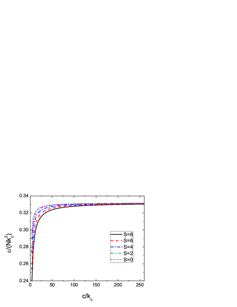
Figure 1: (Color online) The lowest energy spectrum as a function of $c$ and the total spin $S$ without SOC while $N=16$, $\alpha=0$. Here $\varepsilon$ is in units of $Nk_{c}^{2}$ and $c$ is in units of $k_{c}$. The ground state is a ferromagnetic state with $S=8$. These energy levels satisfy $E(S)<E(S^{\prime})$ for $S>S^{\prime}$.

Taking logarithm of the above equations Eq.(11) and Eq.(12), we get

$$\left(k_{j}-\alpha\right)L = 2\pi I_{j}-\sum_{l=1}^{N}2\tan^{-1}\frac{k_{j}-k_{l}}{c}$$ (13)

$$+\sum_{\beta=1}^{M}2\tan^{-1}\frac{k_{j}-\lambda_{\beta}}{c^{\prime}},$$

$$\sum_{j=1}^{N}2\tan^{-1}\frac{\lambda_{\zeta}-k_{j}}{c^{\prime}}=2\pi J_{\zeta}+2\alpha L+\sum_{\beta}2\tan^{-1}\frac{\lambda_{\zeta}-\lambda_{\beta}}{c},$$ (14)

where $I_{j}$ with $j=1,...,N$ and $J_{\zeta}$ with $\zeta=1,...,M$ denote the density quantum numbers and the spin quantum numbers, resepectively. Here $I_{j}$ and $J_{\zeta}$ are integer (half-integer) depending on $N-M$ is odd (even). Taking the periodic property of $\alpha$ into account and letting $I_{j}=I_{j_{0}}-n$ and $J_{\zeta}=J_{\zeta_{0}}-2n$, the above equations could be reduced to

$$\left(k_{j}-\alpha_{0}\right)L = 2\pi I_{j_{0}}-\sum_{l=1}^{N}2\tan^{-1}\frac{k_{j}-k_{l}}{c}$$ (15)

$$+\sum_{\zeta=1}^{M}2\tan^{-1}\frac{k_{j}-\lambda_{\zeta}}{c^{\prime}},$$

$$\sum_{j=1}^{N}2\tan^{-1}\frac{\lambda_{\zeta}-k_{j}}{c^{\prime}} = 2\pi J_{\zeta_{0}}+2\alpha_{0}L$$ (16)

$$+\sum_{\beta=1}^{M}2\tan^{-1}\frac{\lambda_{\zeta}-\lambda_{\beta}}{c}.$$

The corresponding eigenenergy is given by

$$E=\varepsilon-N\alpha^{2}$$ (17)

with $\varepsilon=\sum_{j}k_{j}^{2}$. The total momentum is given by

$$K=\tilde{K}-2S\alpha,$$ (18)

with

$$\tilde{K}=\sum_{j}k_{j}=\frac{2\pi}{L}\left(\sum_{j=1}^{N}I_{j_{0}}-\sum_{\zeta=1}^{M}J_{\zeta_{0}}\right)+2S\alpha_{0}.$$ (19)

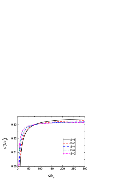
Figure 2: (Color online) The lowest energy spectrum versus $c$ for different $S$ with SOC while $N=16$ and $\alpha=0.95k_{c}/N$. The energy level crossings are shown. In the strong interaction limit, the ground state is transformed to the antiferromagnetic state with $S=0$.

In the absence of the SO coupling, the model is reduced to the SU(2) integrable two-component bosonic model Y. Q. Li ; Fuchs ; Guan Xiwen . For a given $S$, we can get the eigenenergy by solving BA equations. The ground state of this system is ferromagnetic state with $S={N}/{2}$ and the corresponding ground energy is degenerate for $S_{z}\in\left[-S,S\right]$. For a system with $N=16$, we calculate the lowest energies versus the interaction strength $c$ for different total spin $S$, as shown in Fig. 1. Here the parameters $c$ and $E$ are in units of $k_{c}$ and $Nk_{c}^{2}$ where $k_{c}$ is defined as $k_{c}=\pi\rho=\pi{N}/{L}$. Apparently, $E(S)<E(S^{\prime})$ for $S>S^{\prime}$ in the whole regime of interaction strength and the ground state is a ferromagnetic state with maximum $S$. This is different from the case of spin-$1/2$ fermionic gases, where the ground state is antiferromagnetic state with $S=0$ and $E(S)<E(S^{\prime})$ for $S<S^{\prime}$ Lieb-Mattis . In the strong interaction limit, the ground energy for different $S$ go to the same value and become degenerate in the infinite interaction limit Girardeau07 ; GuanLM ; Deuretzbacher .

In the presence of the SO coupling, the energy of ground state for different $S$ can be obtained by solving the BA equations. Fig.2 shows the lowest energy spectrum as the function of the interaction strength for different $S$ with $\alpha={0.95k_{c}}/{N}={0.95\pi}/{L}$. For weak interaction, the energies satisfy $E(S)<E(S^{\prime})$ for $S>S^{\prime}$. When interaction increases, the level crossing would appear and the ferromagnetic state is no longer ground state. For the strong enough interaction, the energy levels fulfill the relation of $E(S)<E(S^{\prime})$ for $S<S^{\prime}$, which is opposite to the law in Fig. 1. That is to say, the ground state of the two-component bosonic system transfers from the ferromagnetic state to the antiferromagnetic state.

III Strong Coupling Limit

To futher investigate how the SO coupling affects the ground state energy, we discuss the strong interaction limit, which permits us to get some analytical expressions for the energy spectrum. In the strong coupling limit, $\lambda_{\zeta}$ are proportional to the interaction strength $c$ whereas $k_{j}$ remain finite GuanLM2 . Applying the Taylor expansion to Eq.(15) and Eq.(16), the equations of $k_{j}$ and $\lambda_{\zeta}$ are simplified as

$$\left(k_{j}-\frac{\tilde{K}}{N}\right) = \frac{2\pi}{L}I_{j_{0}}-\frac{2\pi}{LN}\sum_{j=1}^{N}I_{j_{0}}$$ (20)

$$-\frac{2\rho}{c}\left(k_{j}-\frac{\tilde{K}}{N}\right)\left(1-\frac{v}{2N}\right),$$

$$2N\tan^{-1}\frac{\lambda_{\zeta}}{c^{\prime}}=2\pi J_{\zeta_{0}}+2\alpha_{0}L+\sum_{\beta=1}^{M}2\tan^{-1}\frac{\lambda_{\zeta}-\lambda_{\beta}}{c}$$ (21)

with $v=\sum_{\zeta=1}^{M}\frac{1}{1/4+\left(\lambda_{\zeta}/c\right)^{2}}$. For the state of $M=0$ (or even $M$), $I_{j_{0}}=-\left(N-1\right)/2...\left(N-1\right)/2$, from Eq.(20), we can get

$$\tilde{k}_{j}=\frac{2\pi}{L}I_{j_{0}}-\frac{2\rho}{c}\tilde{k}_{j}\left(1-\frac{v}{2N}\right)$$

with $\tilde{k}_{j}=k_{j}-\frac{\tilde{K}}{N}$. For elementary spin excitations of $M=1$ (odd $M$)Fuchs , $I_{j_{0}}^{1}=-N/2,...,N/2-1$, similarly, $\tilde{k}_{j}$ is given by

$$\tilde{k}_{j}=\frac{2\pi}{L}\left(I_{j_{0}}^{1}+\frac{1}{2}\right)-\frac{2\rho}{c}\tilde{k}_{j}\left(1-\frac{v}{2N}\right)$$

Since $I_{j_{0}}^{1}+\frac{1}{2}=I_{j_{{}_{0}}}$, in general, the equations for quasimomenta $k_{j}$ are represented as

$$k_{j}=\frac{2\pi I_{j_{0}}}{L\left(1+\frac{2\rho}{c}\left(1-\frac{v}{2N}\right)\right)}+\frac{\tilde{K}}{N},$$ (22)

In the strong coupling limit $c/\rho\rightarrow\infty$, $k_{j}=2\pi I_{j_{0}}/L+\tilde{K}/N$. From Eq.(19), it can be seen that $\tilde{K}$ is influenced by the total spin. Without SO coupling, the quasimomenta $\left\{k_{j}\right\}$ are independent on the total spin. In contrast, with SO coupling, the quasimomenta $\left\{k_{j}\right\}$ are shifted by the term $2\alpha_{0}S/N$ for various total spin $S$. Substituting the above equation into $\varepsilon=\sum_{j}k_{j}^{2}$, we get

$$\varepsilon=\frac{\pi^{2}}{3}\frac{N(N^{2}-1)}{L^{2}(1+\frac{2\rho}{c}\left(1-\frac{v}{2N}\right))^{2}}+\frac{\tilde{K}^{2}}{N}.$$ (23)

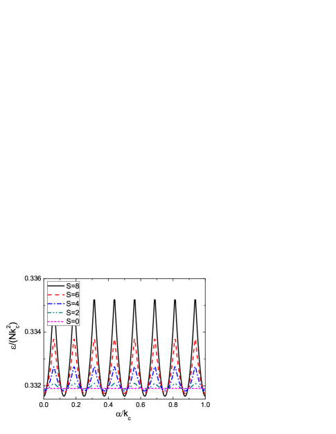
Figure 3: (Color online) The lowest energy spectrum as a function of $\alpha$ for different $S$ with $N=16$, $c/k_{c}=1000$. The SOC strength $\alpha$ is in units of $k_{c}$ and $\alpha\in(0,k_{c})$. The energy changes cyclically versus $\alpha$.

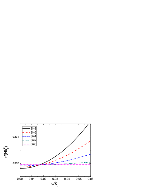
Figure 4: (Color online) An enlargement of the energy spectrum shown in Fig.3 for $\alpha\in(0,k_{c}/N)$. The energy crossings are clearly shown. The ferromagnetic state is the ground state while $\alpha=0$. With the increase of $\alpha$, the ground state is transformed to the antiferromagnetic state.

From Eq.(23), it is shown that the ground energy depends on SO coupling parameter $\alpha$ in two aspects. First, the spin rapidity $\lambda_{\zeta}$ is dependent on $\alpha_{0}$ from its self-consistent Eq.(21). Second, from Eq.(19), $\tilde{K}$ is the function of $\alpha_{0}$. In the strong interaction limit $c/\rho\rightarrow\infty$, as $\rho/c\rightarrow 0$, the contribution of spin rapidity can be ignored. Only the term $\tilde{K}^{2}/N$ will affect the energy for different $S$.

In the case of even $N$ and $M$, the quantum numbers $J_{\zeta_{0}}=-(M+1)/2-\zeta$ with $\zeta=1...M$. Here from Eq.(19), $\tilde{K}=2S\alpha_{0}$ and $\tilde{K}$ is proportional to $S$. From Eq.(22), while $c/\rho\rightarrow\infty$, the quasimomenta satisfy $k_{j}=2\pi I_{j_{0}}/L+2\alpha_{0}S/N$. From Eq.(23), the energy is given by

$$\frac{\varepsilon}{k_{c}^{2}N}=\frac{N^{2}-1}{3N^{2}}+\left(\frac{\alpha_{0}}{k_{c}}\right)^{2}\left(\frac{2S}{N}\right)^{2}.$$ (24)

It is obvious that the energy takes lowest value for $S=0$. The SO coupling favors antiferromagnetic state as the ground state. As large but finite interaction, the energy level crossings occur due to competition between SO coupling and interaction. In Fig. 3, we show the lowest energy levels versus $\alpha$ in the strongly interacting case with $c/k_{c}=1000$, where the SO coupling parameter is chosen in the range of $\alpha/k_{c}\in\left(0,1\right)$. The cyclical change of energy with the increase of $\alpha$ coincides with our previous discussion. In Fig. 4, the lowest energy spectrum is plotted versus $\alpha$ with the range $\alpha/k_{c}\in\left(0,\pi/L\right)$ which is the half of the period of $\alpha$ in Fig. 3. When $\alpha=0$, the energy levels fulfill $E(S)<E(S^{\prime})$ for $S<S^{\prime}$. With the increase of $\alpha$, energy level crossings appear for different $S$. When $\alpha$ is large enough, the energy levels satisfy the opposite law. After the crossing, the energy differences for various $S$ become larger with increasing $\alpha$.

Before ending the paper, we would like to give a remark on the interacting spin-$1/2$ fermionic model with SO coupling, for which the SO coupling induced level crossing is absent. As for the 1D interacting spin-$1/2$ fermionic gas CNYang , the ground state is an antiferromagnetic state ($S=0$) in the absence of SO coupling. In the presence of SO coupling, one can still use the gauge transformation to transform the problem into an integrable spin-$1/2$ fermionic model with a spin-dependent twisted boundary condition Shun Uchino ; B. S. Shastry , and the system is determined by the following BA equations

$$\left(k_{j}-\alpha\right)L=2\pi I_{j}-\sum_{\zeta=1}^{M}2\tan^{-1}\frac{k_{j}-\lambda_{\zeta}}{c^{\prime}},$$ (25)

$$\sum_{j=1}^{N}\tan^{-1}\frac{\lambda_{\zeta}-k_{j}}{c^{\prime}}=2\pi J_{\zeta}-2\alpha L+\sum_{\beta=1}^{M}2\tan^{-1}\frac{\lambda_{\zeta}-\lambda_{\beta}}{c}.$$ (26)

In the strong interaction limit, the energy is

$$\varepsilon=\frac{\pi^{2}}{3}\frac{N(N^{2}-1)}{L^{2}\left(1+\frac{v}{cL}\right)^{2}}+\frac{\tilde{K}^{2}}{N}.$$

Similar to the bosonic case, the SO coupling still favors the antiferromagnetic state as the ground state. The SO coupling does not lead to level crossing for spin-$1/2$ fermions, i.e., the ground state will always be an antiferromagnetic state.

IV Summary

In summary, we have analytically solved 1D interacting spin-1/2 bosonic gases with SO coupling. As the effect of SO coupling can be absorbed into the twisted boundary condition, we get the exact solution to this system by BA method and find that the corresponding eigenenergies are periodically dependent on the SO coupling. The interplay between interaction and SO coupling has revealed the existence of energy level crossing and the ground state phase transition from the ferromagnetic state to antiferromagnetic state.

References

• (1) B. Paredes, et al., Nature 429, 277 (2004).
• (2) T. Kinoshita, T. Wenger and D. S. Weiss, Science 305, 1125 (2004).
• (3) M. A. Cazalilla, R. Citro, T. Giamarchi, E. Orignac, and M. Rigol, Rev. Mod. Phys. 83, 1405 (2011).
• (4) X.-W. Guan, M. T. Batchelor and C. H. Lee, arXiv:1301.6446.
• (5) Y.-J. Lin et al., Nature(London) 462, 628 (2009); Y.-J. Lin et al., Nat. Phys. (London) 7, 531 (2011); Y.-J. Lin, K. J. Garcis , I. B. Spielman, Nature(London) 83, 471 (2011).
• (6) P. Wang, Z.-Q. Yu, Z. K. Fu, J. Miao, L. H. Huang, S. J. Chai, H. Zhai, and J. Zhang, Phys. Rev. Lett. 109, 095301(2012).
• (7) L. W. Cheuk, A, T. Sommer, Z. Hadzibabic, T. Yefsah, W. S. Bakr, and M. W. Zwierlein, Phys. Rev. Lett.109, 095302(2012).
• (8) J. Higbie and D. M. Stamper-Kurn, Phys. Rev. Lett. 88, 090401 (2002).
• (9) X. L. Qi and S. C. Zhang, Phys. Rev. Lett. 52, 2111 (2010).
• (10) M. Z. Hasan and C. L. Kane, Rev. Mod. Phys. 82, 3045 (2010).
• (11) C. Wang, C. Gao, C.-M. Jian, and H. Zhai, Phys. Rev. Lett. 105, 160403 (2010).
• (12) T.-L. Ho and S. Z.Zhang, Phys. Rev. Lett. 107, 150403 (2011).
• (13) W. Zheng and Z. Li, Phys. Rev. A 85, 053607 (2012).
• (14) T. Ozawa and G. Baym, Phys. Rev. Lett. 109, 025301 (2012).
• (15) Q. Z. Zhu, C. W. Zhang, B. Wu, EPL 100, 50003 (2012).
• (16) C. J. Wu, I. Mondragon-Shem and X. F. Zhou, Chin. Phys. Lett. 28, 097102 (2011).
• (17) B. Ramachandhran B. Opanchuk, X.-J. Liu, H. Pu, P. D. Drummond and Hui Hu, Phys. Rev. A 85, 023606 (2012).
• (18) S. Sinha, R. Nath, and L. Santos, Phys. Rev. Lett. 107, 270401 (2011)
• (19) X.-Q. Xu and J. H. Han, Phys. Rev. Lett. 107, 200401 (2011).
• (20) J. Radi’c, T. Sedrakyan, I. B. Spielman, and V. Galitski, Phys. Rev. A 84, 063604 (2011).
• (21) Z. F. Xu, R. L u, and L. You, Phys. Rev. A 83, 053602 (2011); Z. F. Xu, Y. Kawaguchi, L. You, and M. Ueda, Phys. Rev. A 86, 033628 (2012).
• (22) Y. Q. Li, S. J. Gu, Z.J. Ying and U. Echern, Europhys. Lett. 61, 368 (2003).
• (23) J. N. Fuchs, D. M. Gangardt, T. Keilmann, and G. V. Shlyapnikov, Phys. Rev. Lett. 95, 150402 (2005).
• (24) X. W. Guan and M. T. Batchelor and M. Takahashi, Phys. Rev. A 76, 043617 (2007).
• (25) Y. J. Hao, Y. B. Zhang, X. W. Guan and S. Chen, Phys. Rev. A 79, 033607 (2009).
• (26) S. Uchino and N. Kawakami, Phys. Rev. A 85, 013610 (2012).
• (27) B. S. Shastry and B. Sutherland, Phys. Rev. Lett. 65, 243 (1990).
• (28) E. H. Lieb and D. Mattis, Phys. Rev. 125, 164 (1962).
• (29) M. D. Girardeau and A. Minguzzi, Phys. Rev. Lett. 99, 230402 (2007).
• (30) L. Guan, S. Chen, Y. Wang, and Z. Q. Ma, Phys. Rev. Lett. 102, 160402 (2009).
• (31) F. Deuretzbacher, K. Fredenhagen, D. Becker, K. Bongs, K. Sengstock, and D. Pfannkuche , Phys. Rev. Lett. 100, 160405 (2008).
• (32) L. Guan and S. Chen, Phys. Rev. Lett. 105, 175301 (2010).
• (33) C. N. Yang, Phys. Rev. Lett. 19, 1312 (1967).