Selection theory of free dendritic growth in a potential flow

Abstract

The Kruskal-Segur approach to selection theory in diffusion-limited or Laplacian growth is extended via combination with the Zauderer decomposition scheme. This way nonlinear bulk equations become tractable. To demonstrate the method, we apply it to two-dimensional crystal growth in a potential flow. We omit the simplifying approximations used in a preliminary calculation for the same system [T. Fischaleck, K. Kassner, EPL 81, 54004 (2008)], thus exhibiting the capability of the method to extend mathematical rigor to more complex problems than hitherto accessible.

I Introduction

Pattern formation is ubiquitous in nature. Snowflakes constitute an everyday-paradigm of a self-organized structure, apparently the first that was the subject of scientific study kepler1611 . Any physical pattern possesses at least one characteristic length scale, and if it is dynamic, it also has a characteristic time scale. The foremost task of scientific endeavour in the field of pattern formation is to explain the emergence of these scales and to determine them quantitatively. Since systems with linear dynamics will, due to the superposition principle, not normally single out a particular length scale, an essential ingredient of pattern-forming systems is the nonlinearity of their dynamics .

As it turns out, snowflake-like structures – dendritic morphologies – also arise at microscopic scales in the casting of metals and they determine structural properties such as the strength of the material, which imparted considerably more importance to scientific preoccupation with them than just fundamental interest would have.

The first models of dendritic crystal growth assumed transport of heat away from or material to, the growing nucleus to be simply diffusive, so the term diffusion-limited growth was coined. Understanding the selection of dynamical features such as a basic length scale and the growth velocity turned out to be remarkably difficult even within these simplifying models. Almost forty years passed between Ivantsov’s approximate solution ivantsov47 that did not exhibit selection and the development of an analytic theory explaining the mechanism of structure selection langer86b ; caroli86 ; benamar86 . This may seem even more surprising considering that the bulk equations of diffusion-limited systems are linear and the nonlinearity of the dynamics emerges solely via the equations of motion for the two-phase interface. In fact, the analytic approaches developed had to rely heavily on this linearity.

Ivantsov’s theory, neglecting surface tension at the boundary between the melt and the solid, predicts only the product of the tip radius of a dendrite and its growth velocity, as a function of the undercooling. In experiments, the undercooling determines both quantities separately. A decisive step towards the solution was the insight that without surface tension the problem is ill-posed benjacob84b ; kessler85 and that the capillary length has to be taken into account, even if it is much smaller than any length scale of the arising pattern. Surface tension regularizes the mathematical problem and drastically alters the solution space. Without surface tension, there is a continuum of parabolic needle crystal solutions. With isotropic surface tension, there are no solutions with a shape close to one of these Ivantsov parabolas (or paraboloids), no matter how small the surface tension, a fact that testifies to the singular nature of the “perturbation” surface tension. With anisotropic surface tension, the continuum of Ivantsov solutions is reduced to a discrete set, with the fastest of the needle crystal solutions being the only linearly stable one . Hence, the selection problem is broken down into two parts – an existence problem for a discrete set of solutions and the stability analysis singling out one element of the set as the one that should be observed. A completely analogous theory was developed for Saffman-Taylor fingers in viscous fingering hong86 ; shraiman86 ; combescot86 , where selection is also due to surface tension, albeit not, of course, to its anisotropy.

These theories were two-dimensional, just as the original numerical work giving evidence for a selection mechanism based on solvability meiron86a ; kessler86 ; kessler86d . Three-dimensional situations considered initially referred to axisymmetric crystals kessler86 ; barbieri87 , hence were not very realistic. Later, steps were taken to extend the theory towards non-axisymmetric needle-crystal shapes kessler87 ; kessler88a and eventually, an analytic theory was developed for the fully non-axisymmetric case benamar93 ; brener93a ; all the necessary elements of the final complete theory were not present before Ref. brener93a, .

From the outset, two different analytic approaches were pursued. With the first method, the equation of motion of the two-phase interface is linearized, which leads to an integro-differential equation in non-local problems (such as dendritic growth or viscous fingering). Using Fredholm’s alternative, a solvability condition is derived that is satisfied only by a discrete set of values of the selection parameter (a nondimensionalized surface tension or its inverse) langer86 ; hong86 ; barbieri87 . The second approach, pioneered by Kruskal and Segur kruskal91 , consists in solving the interface equation far from singular points in the complex plane via a perturbation expansion in terms of the small selection parameter and in the vicinity of these points via a scale transformation and reduction to a local equation. The two solutions then have to be asymptotically matched to obtain a globally valid solution. Parameter relationships established in the matching procedure yield the selection criterion benamar86 ; tanveer89 ; benamar90 ; brener91 ; tanveer00 . There is general agreement that only the second approach is mathematically rigorous combescot86 ; hong87 ; barbieri89 ; tanveer89 . The linearization of the first method introduces approximations that normally will not invalidate the scaling relations obtained; but it will not reproduce their prefactors correctly nor provide a globally valid approximate solution. Moreover, if the equations contain more than one small parameter (say, a kinetic coefficient or a characteristic number describing the flow, besides the usual selection parameter), the linearization may produce even worse results due to the structural instability of the problem tanveer89 .

In both approaches, it is necessary to first derive an (integro-differential) equation for the interface position depending on a single independent variable. This can be achieved, e.g., by eliminating the bulk field variables via conformal mapping (in the viscous fingering case) or using Green’s function methods (in crystal growth). These techniques are applicable only for linear bulk equations, which seemed to preclude utilization of the method for convection problems.

For a long time, the only exception to this restriction has been the work on two-dimensional crystal growth in an Oseen flow by Bouissou and Pelcé bouissou89b . To obtain the selection criterion, they used a method, outlined in Ref. pelce88, , which is closely related to the first of the two approaches mentioned, hence not rigorous. Their method has recently been extended by Alexandrov et al. alexandrov10 to include solute diffusion. The equation of motion for the deviation of the solution from that of the problem without surface tension is simplified in the style of a linear stability analysis which allows to avoid the derivation of an integro-differential equation. Moreover, the adjoint linear operator is constructed heuristically in Fourier space to obtain a solvability condition in the spirit of the Fredholm alternative, a procedure that may introduce additional (possibly problematic) approximations.

A different method, having the potential of achieving the same level of rigor for problems with nonlinear bulk equations as the asymptotic matching approach, was recently introduced fischaleck08 ; fischaleck08b . It consists in a combination of Zauderer’s decomposition scheme zauderer78 for partial differential equations with the Kruskal-Segur approach. Zauderer decomposition is the step allowing reduction of nonlinear bulk equations to an interface equation and thus circumventing the necessity of an exact integral equation, available only for linear bulk equations. Reference fischaleck08, , dealing with potential flow, was more or less a proof of concept, in which we copiously used additional approximations to simplify the result to an easily digestable form, allowing to map it in the end to the flowless finite Péclet number case treated by Ben Amar benamar90 . The main purpose of the present paper is to remove these approximations, which renders the treatment more complex, but does not impose insurmountable obstacles. Of course, the mapping obtained gets lost, because it was only approximate. Clearly, potential flow is not a very realistic assumption, but it has the advantage that the unperturbed problem is exactly solvable; the analog of Ivantsov’s analytic solution exists. This is different in the case treated by Bouissou and Pelcé bouissou89b , where already the zeroth-order problem is solved within an approximation, replacing the Navier-Stokes equations with the Oseen problem (which in two dimensions does not even give a uniform approximation to the true flow saville88 ). We will consider more realistic flows and a better approach than the Oseen approximation in a later publication.

The paper is organized as follows. In Sec. II, the model equations are given. They are nondimensionalized and rewritten in parabolic coordinates in Sec. III. Section IV gives the analog of the Ivantsov solution in the presence of a potential flow. Then the method of Zauderer decomposition is explained in Sec. V, allowing us to reduce the set of partial differential equations of the full problem to an integro-differential equation for the interface alone, without losing the terms decisive for solvability theory. Next, the decomposed equations are solved to first order (in the small parameter $\sigma^{2/7}$) in Sec. VI. Near the solid-liquid interface, the relevant behavior beyond all orders of regular perturbation theory is obtained in Sec. VII from a WKB analysis. On the other hand, in Sec. VIII, the asymptotic Kruskal-Segur reduction to a locally valid equation, applicable near a singularity in the complex plane, is carried out. It leads to a nonlinear integro-differential equation constituting an eigenvalue problem. The numerical solution of this eigenvalue problem determines the selected velocity (and other properties) of the needle crystal. Detailed results are given for a set of parameters corresponding to a particular experimental system, which however does not exhibit potential flow, so the comparison is only qualitative. Some conclusions are offered in Sec. IX. A few general calculations and slightly elaborate mathematical conversions are relegated to two appendices.

II Model equations

Heat transport in the liquid and solid phases is described by the diffusion-advection equations

$$\frac{\partial T}{\partial{t}}+\left(\mathbf{w}\cdot\nabla\right)T=D\nabla^{2}T$$ (1)

with $\mathbf{w}$ the flow velocity in the liquid and $\mathbf{w}\equiv 0$ in the solid. The advection term coupling the temperature and flow equations renders the bulk problem nonlinear, despite the simplifying assumption of potential flow made below (which reduces the flow description to a linear equation). As the notation suggests, we assume the thermal diffusivity $D$ to be the same in both phases (symmetric model). We consider an incompressible flow, which means that a stream function can be introduced. In two dimensions, its defining equation takes the form

$$\mathbf{w}=\nabla\times(\psi\mathbf{e}_{z})=\psi_{y}\mathbf{e}_{x}-\psi_{x}\mathbf{e}_{y}\>.$$ (2)

Because $\psi$ depends on $x$ and $y$ only, we obtain $\nabla\times\mathbf{w}=-\nabla^{2}\psi\,\mathbf{e}_{z}$ and taking the flow to be potential, we have

$$\nabla^{2}\psi=0\>.$$ (3)

When specializing Eq. (1) to one of the phases, we will denote the temperature variable by $T^{l}$ and $T^{s}$ in the liquid and the solid, respectively. Equations (2) and (3) are the bulk equations of motion for the flow.

Because we are looking for steady-state solutions, we need not prescribe detailed initial conditions. We must however specify boundary conditions for each of the bulk equations. At infinity in either the liquid or solid we require homogeneous Dirichlet boundary conditions for the temperature fields, i.e., we set the temperature constant:

$$T^{l}(\mathbf{x}) \to T_{\infty} \text{for }d(\mathbf{x},\Gamma)\to\infty\>,$$ (4a)

$$T^{s}(\mathbf{x}) \to T_{M} \text{for }d(\mathbf{x},\Gamma)\to-\infty\>.$$ (4b)

Herein, $\Gamma$ is the interface and $d(\mathbf{x},\Gamma)$ denotes a signed distance function, increasing towards the liquid. $T_{M}$ is the bulk melting temperature of the solid, and for crystal growth to occur in a pure system, we must have $T_{\infty}<T_{M}$. The dimensionless parameter characterizing this undercooling is

$$\Delta=\frac{T_{M}-T_{\infty}}{L/c_{p}}\>,$$ (5)

where $L$ and $c_{p}$ are the latent heat and specific heat, both referred to a unit volume.

Moreover, there are boundary conditions at the interface, reading

$$T^{s}|_{\Gamma}=T^{l}|_{\Gamma}\>,$$ (6a)

$$T^{l}|_{\Gamma}=T_{M}-\frac{L}{c_{p}}d_{0}\kappa a(\theta)\>,$$ (6b)

$$LV_{n}=Dc_{p}\left[\nabla T^{s}|_{\Gamma}-\nabla T^{l}|_{\Gamma}\right]\cdot\mathbf{n}\>.$$ (6c)

Equation (6a) describes continuity of the temperature across the interface, Eq. (6b) is the Gibbs-Thomson condition giving the equilibrium temperature of a melt-crystal interface with curvature $\kappa$. That is, we assume kinetic effects to be negligible, implying local thermal equilibrium at the interface. If the interface is given by $y=h(x)$, then $\kappa=-h^{\prime\prime}(x)/\left(1+h^{\prime}(x)^{2}\right)^{3/2}$. $d_{0}$ is the average capillary length,

$$d_{0}=\gamma_{0}\frac{T_{M}c_{p}}{L^{2}}\>,$$ (7)

where $\gamma_{0}$ is the angular average of the orientation dependent surface tension $\gamma(\theta)$. $\theta$ is the angle of the interface normal with some fixed direction, for example the direction of the $y$ axis. From the thermodynamics of interfaces we know nozieres92 that the angular dependence of the non-averaged capillary length is not that of the surface tension but that of the surface stiffness $\gamma(\theta)+\gamma^{\prime\prime}(\theta)$. This is described by the factor $a(\theta)\equiv(\gamma(\theta)+\gamma^{\prime\prime}(\theta))/\gamma_{0}$. For simplicity, we will assume fourfold anisotropy here, described by a single harmonic, i.e.

$$a(\theta)=1-\beta\cos(4\theta)\>.$$ (8)

From a mathematical point of view, Eqs. (6a,6b) together with the boundary conditions at infinity and some initial condition for the two temperature fields are sufficient to solve the diffusion problem in the two phases, with given flow field and interface position. However, the interface position is a priori unknown, its determination is part of the problem. Therefore, an additional interface equation is needed. This is the third boundary condition, the Stefan condition (6c). Physically, it follows from energy conservation across the interface. $V_{n}$ is the interface normal velocity and the left-hand term describes latent heat production due to advancement of the interface, whereas the right-hand side gives the sum of the heat currents into the solid and liquid phases. The normal vector $\mathbf{n}$ points from the solid into the liquid.

The flow field $\mathbf{w}$ is dynamic only in the liquid. We need a boundary condition at infinity, where we impose a constant flow directed opposite to the growth direction of the needle crystal:

$$\mathbf{w}(\mathbf{x}) \to-U\mathbf{e}_{y} \text{for }d(\mathbf{x},\Gamma)\to\infty\>.$$ (9)

Because we have potential flow, we cannot impose conditions for all three components of the flow velocity at the interface; the Laplace equation for the stream function does not admit prescription of more than one scalar quantity. Physically, this is reasonable, since potential flow is frictionless, hence we cannot prescribe the tangential velocity at the interface, there is no no-slip condition. The normal velocity, on the other hand, follows from mass conservation. We assume the simplest case, viz. equal mass densities in the solid and the liquid. Then the liquid is neither sucked towards the solid (which would be the case if the density of the solid were higher than that of the liquid), nor ejected from it. Since the solid does not move , the normal velocity of the liquid must be zero:

$$\mathbf{n}\cdot\mathbf{w}(\mathbf{x})|_{\Gamma}=0\>.$$ (10)

Equations (1) through (10), supplemented by initial conditions for all the fields, constitute the complete mathematical description of an idealized physical system. Requiring the solution to be stationary and to correspond to a crystal growing at constant velocity $V$ along the $y$ direction we may replace $V_{n}$ in Eq. (6c) by $V\mathbf{e}_{y}\cdot\mathbf{n}=Vn_{y}$. Transforming to a moving frame of reference,

$$\mathbf{r} \to\mathbf{r}+Vt\mathbf{e}_{y}\>,$$ (11a)

$$\mathbf{w} \to\mathbf{w}+V\mathbf{e}_{y}\>,$$ (11b)

in which the interface is at rest, all time derivatives $\partial_{t}$ get replaced by $-V\partial_{y}$. Note that due to the transformation of $\mathbf{w}$, Eq. (1) is invariant under this change of frame. Nevertheless, the time derivative can be dropped after the transformation, because we seek a time-independent solution. Moreover, the “flow velocity in the solid” becomes $-V\mathbf{e}_{y}$ by virtue of the transformation.

III Parabolic coordinates and nondimensionalization

A family of exact analytic steady-state solutions to the model equations exists for vanishing capillary length and, similar to Ivantsov’s solution in the flowless case, the crystal interface is parabolic das84 ; benamar88c ; cummings99 . Therefore, it is useful to introduce parabolic coordinates. We employ conformal parabolic coordinates

$$x=\eta\xi\>,\qquad y=\frac{1}{2}\left(\eta^{2}-\xi^{2}\right)\>,$$ (12)

their advantage being equality of the scale factors $g_{\xi}=g_{\eta}=\sqrt{\xi^{2}+\eta^{2}}$. In the appendix, some of the transformation formulas and a graphical representation of the coordinate lines are given.

To nondimensionalize the equations, we use the tip radius $\rho$ of the Ivantsov like solution, defined as the inverse of the curvature at the tip, as a length scale. The corresponding diffusion time $\rho^{2}/D$ is taken as a time scale

$$x,y\to\rho x,\rho y,\;\kappa\to\frac{\kappa}{\rho}\,,\quad t\to\frac{\rho^{2}}{D}t\>.$$ (13)

Note that this implies $\xi$ and $\eta$ to scale with $\sqrt{\rho}\,$: $\xi,\eta\to\sqrt{\rho}\,\xi,\sqrt{\rho}\,\eta$.

The nondimensional form of the flow velocity follows immediately

$$\mathbf{w}\to\frac{D}{\rho}\mathbf{w}\>.$$ (14)

(This implies $\psi\to D\psi$.) The nondimensional flow velocity at infinity then becomes

$$P_{f}\equiv\frac{\rho U}{D}\>,$$ (15)

the so-called flow Péclet number. Moreover, it will turn out useful to include the growth Péclet number

$$P_{c}\equiv\frac{\rho V}{D}\>,$$ (16)

into the prescription for nondimensionalization of temperature

$$T\to T_{M}+\frac{L}{c_{p}}P_{c}T\>,$$ (17)

which means that the nondimensional temperature in the liquid approaches $-\Delta/P_{c}$ at infinity.

With these transformations and dropping time derivatives, as we are interested in stationary solutions, we obtain the following set of bulk equations

$$\psi_{\eta}T^{l}_{\xi}-\psi_{\xi}T^{l}_{\eta} =T^{l}_{\xi\xi}+T^{l}_{\eta\eta}\,,$$ (18a)

$$P_{c}\left(\xi T^{s}_{\xi}-\eta T^{s}_{\eta}\right) =T^{s}_{\xi\xi}+T^{s}_{\eta\eta}\,,$$ (18b)

$$\psi_{\xi\xi}+\psi_{\eta\eta} =0\>.$$ (18c)

The boundary conditions for the fields at the interface now read

$$T^{s} =T^{l}\>,$$ (19a)

$$T^{l} =-\frac{1}{2}\sigma\kappa a(\theta)\>,$$ (19b)

$$\left[\xi\eta_{s}\right]^{\prime} =-\eta_{s}^{\prime}\left(T_{\xi}^{s}-T_{\xi}^{l}\right)+T_{\eta}^{s}-T_{\eta}^{l}\>,$$ (19c)

$$\psi_{\xi}+\eta_{s}^{\prime}\psi_{\eta} =P_{c}\left(\eta_{s}+\eta_{s}^{\prime}\xi\right)\>,$$ (19d)

where $\eta_{s}(\xi)$ is the interface position, a prime means a derivative with respect to $\xi$ along the interface, and

$$\sigma=\frac{2d_{0}}{\rho P_{c}}$$ (20)

is the selection or stability parameter. (In order not to overburden the notation, we have dropped the qualifier $|_{\Gamma}$ next to the fields and their derivatives, indicating that these quantities have to be evaluated at the interface position.)

Finally, the boundary conditions at infinity may be written (see Fig. 5)

$$T^{l} \to-\frac{\Delta}{P_{c}} (\eta\to\infty)\>,$$ (21a)

$$T^{s} \to 0 (\eta<1,\>\left\lvert\xi\right\rvert\to\infty)\>,$$ (21b)

$$\psi \sim\left(P_{f}+P_{c}\right)\eta\xi (\eta\to\infty)\>,$$ (21c)

the last equation being an asymptotic equality bender78 .

IV Exact solution in the absence of surface tension

If we neglect surface tension in the spirit of Ivantsov, eqs. (19a,19b) tell us that with vanishing capillary length the interface becomes an isotherm, $T^{l}|_{\Gamma}=T^{s}|_{\Gamma}=0$. Assuming it to be a coordinate line suggests the temperature field to depend on one of the coordinates only, i.e. $T=T(\eta)$. Inserting this into (18a,18b), we have

$$-\psi_{\xi}T^{l}_{\eta} =T^{l}_{\eta\eta}\>,$$ (22a)

$$-P_{c}\eta T^{s}_{\eta} =T^{s}_{\eta\eta}\>.$$ (22b)

In view of boundary condition (21b), we see that the second equation is solved by $T^{s}\equiv 0$. The first can have a purely $\eta$ dependent solution only if

$$\psi=\xi f(\eta)\>.$$ (23)

Inserting this into (18c), we find

$$f^{\prime\prime}(\eta)=0\quad\Rightarrow\quad f(\eta)=c_{1}\eta+c_{2}\>,$$ (24)

with constants $c_{1}$ and $c_{2}$ to be determined from the two boundary conditions (19d,21c). By assumption, the interface is at $\eta_{s}(\xi)\equiv 1$, so (19d) simplifies into $\psi_{\xi}(1)=P_{c}$. We find $c_{1}=P_{f}+P_{c}$ and $c_{2}=-P_{f}$. Therefore,

$$\psi=\psi^{\text{Iv}}=\xi\left(P_{c}\eta+P_{f}(\eta-1)\right).$$ (25)

This leaves us with the ordinary second-order differential equation (22a) $T^{l}_{\eta\eta}+\left(P_{c}\eta+P_{f}(\eta-1)\right)T^{l}_{\eta}=0$ subject to the boundary conditions $T^{l}(1)=0$ and (21a). The solution is straightforward:

$$T^{l}=T^{\text{Iv}}(\eta)=-\mathrm{e}^{\frac{P_{c}}{2}}\int\limits_{1}^{\eta}\mathrm{e}^{-\frac{P_{c}}{2}\eta^{\prime 2}-\frac{P_{f}}{2}\left(\eta^{\prime}-1\right)^{2}}\mathrm{d}\eta^{\prime}\>,$$ (26)

where $P_{c}$ is determined as a function of $\Delta$ and $P_{f}$ from

$$\frac{\Delta}{P_{c}}=\mathrm{e}^{\frac{P_{c}}{2}}\int\limits_{1}^{\infty}\mathrm{e}^{-\frac{P_{c}}{2}\eta^{\prime 2}-\frac{P_{f}}{2}\left(\eta^{\prime}-1\right)^{2}}\mathrm{d}\eta^{\prime}\>.$$ (27)

In the limit $P_{f}\to 0$, this becomes identical to the usual Ivantsov relation for diffusion-limited dendritic growth, whereas for $P_{c}\ll P_{f}$ we can evaluate the formula analytically, which yields $\Delta=P_{c}\sqrt{\pi/2P_{f}}$. The selection problem arises in the same way here as in the flowless case: only $P_{c}$ is determined, given the undercooling and the imposed flow, by the Ivantsov-like solution. Given $P_{c}$, we can calculate the product of the growth rate $V$ and the tip radius $\rho$ but not both quantities separately. Ivantsov’s approach eliminates the parameter $\sigma$ from the equations. As (20) tells us, we may calculate $\rho$ once we know $\sigma$ and $P_{c}$. So the aim must be to include $\sigma$ into the theory and to obtain a value for it.

For easy reference, we will call the solution (25) – (27) the flow-Ivantsov solution.

V Zauderer decomposition and continuation to the complex plane

The approach to be followed is singular perturbation theory about the flow-Ivantsov solution . Thus, we shall consider small deviations from it

$$T\to T^{\text{Iv}}+T\quad\text{and}\quad\psi\to\psi^{\text{Iv}}+\psi\>,$$ (28)

but we will be careful to avoid illegitimate linearizations. In particular, we will not linearize terms containing derivatives of the interface position.

In this first approach, we shall restrict ourselves to the limit of small growth Péclet number, i.e., $P_{c}\ll 1$. As it turns out, interesting results for the selection parameter arise only, if we also assume $P_{c}\ll P_{f}$. In particular, this means that terms with a factor of $P_{c}$ will be neglected in the exponentials of Eqs. (26) and (27).

The diffusion-advection equation (18a) then becomes an inhomogeneous equation for the temperature deviation, in the liquid, from the flow-Ivantsov solution

$$T^{l}_{\xi\xi}+T^{l}_{\eta\eta} -\left(\psi_{\eta}+\xi P_{f}\right)T^{l}_{\xi}$$

$$+\left(\psi_{\xi}+P_{f}(\eta-1)\right)T^{l}_{\eta}=\psi_{\xi}\mathrm{e}^{-\frac{P_{f}}{2}\left(\eta-1\right)^{2}}\>.$$ (29)

The only approximation in this equation is that $P_{c}$ has been set equal to zero. All field nonlinearities are still present.

In the solid (Eq. (18b)), we just drop the terms multiplied by $P_{c}$ and obtain a Laplace equation

$$T^{s}_{\xi\xi}+T^{s}_{\eta\eta}=0\>,$$ (30)

and Eq. (18c), being linear, remains formally unchanged,

$$\psi_{\xi\xi}+\psi_{\eta\eta}=0\>,$$ (31)

but the meaning of $\psi$ is now different (it is the deviation of the stream function from its form in the flow-Ivantsov solution).

To rewrite the boundary conditions, we set $\eta_{s}=1+h(\xi)$. While it is legitimate to view $h(\xi)$ as a small quantity, this may not be true for $h^{\prime}(\xi)$ and higher derivatives. Expanding (19a) about the flow-Ivantsov solution, we have $T^{\text{Iv}}|_{\Gamma}+T^{l}|_{\Gamma}=\partial_{\eta}T^{\text{Iv}}|_{\eta=1}\,h+T^{l}(\xi,1)=T^{s}|_{\Gamma}=T^{s}(\xi,1)$. Later, we will need the derivative of the interface temperature with respect to $\xi$. We are then not allowed to simply take the partial derivative of the temperature field with respect to $\xi$, which would give $T^{l}_{\xi}-h^{\prime}(\xi)=T^{s}_{\xi}$ (because $\partial_{\eta}T^{\text{Iv}}|_{\eta=1}=-1$). Actually, the derivative must be taken along the interface, so we obtain $T^{l}_{\xi}+T^{l}_{\eta}h^{\prime}(\xi)-h^{\prime}(\xi)=T^{s}_{\xi}+T^{s}_{\eta}h^{\prime}(\xi)$ instead. Keeping this proviso in mind, we may use the simpler form before differentiation as the shortest description of the appropriate boundary condition. The full set of interface boundary conditions then reads

$$T^{s}+h =T^{l}\>,$$ (32a)

$$T^{s} =-\frac{1}{2}\sigma\kappa a(\theta)\>,$$ (32b)

$$\left[\xi h\right]^{\prime} =\left(\frac{\partial}{\partial{\eta}}-h^{\prime}\frac{\partial}{\partial{\xi}}\right)\left(T^{s}-T^{l}\right)\>,$$ (32c)

$$\psi_{\xi}+h^{\prime}\psi_{\eta} =-P_{f}\left[h\xi\right]^{\prime}\>.$$ (32d)

All of these are evaluated at $\eta=1$, but if they are to be differentiated, then this has to be done before setting $\eta=1$ and field derivatives with respect to $\eta$ will arise.

Zauderer’s asymptotic decomposition zauderer78 is a projection scheme reducing the solution of a system of partial differential equations (PDEs) to the solution of a series of first-order equations. These may be decoupled within a perturbative approach, if a small parameter or slow variable is available. (Otherwise, the series of first-order equations does not offer any simplification over the original system of PDEs.) Originally conceived for hyperbolic equations, the method generalizes to elliptic systems in the complex plane.

Asymptotic decomposition seems to have largely passed into oblivion (at least in the physics world), possibly because often multi-scale expansions are superior to it, leading to more easily tractable equations. Nevertheless, for the problem considered here, Zauderer decomposition is particularly well-suited, not losing information about transcendentally small terms (if the “principal part” zauderer78 of the set of equations is chosen correctly).

In fischaleck08 , we discussed that in the case of purely diffusive transport and in the limit of small growth Péclet number, Zauderer decomposition of the transport equations is equivalent to their factorization

$$\left(\partial_{\xi}+\mathrm{i}\partial_{\eta}\right)T^{l}=0\>,\quad\left(\partial_{\xi}-\mathrm{i}\partial_{\eta}\right)T^{s}=0\>,$$ (33)

and that a few simple manipulations of these partial differential equations using the boundary conditions lead to a local equation for the interface position $h(\xi)$,

$$\sigma a(\theta)\kappa=(1-\mathrm{i}\xi)h(\xi)\>.$$ (34)

This equation contains the complete information needed to compute the mismatch function that has to be zero at the tip of the needle crystal for selection to be possible. Near the singularity $\xi=-\mathrm{i}$ in the complex plane, Eq. (34) describes the dominant behavior of the solution.

Equations (33) are, due to their simplicity, well-suited for a discussion of the strategy of our approach. Typically, Zauderer decompostion produces, from the basic partial differential equations of the problem, a leading-order or “principal-part” equation in each domain that is first order and easily solvable (for example by the method of characteristics). The complete solution will be a sum of this leading term and other contributions that may be calculated in subsequent steps of the perturbative scheme. In the simple case considered here for explanatory purposes, the temperature field satisfies the Laplace equation factorizing in the complex plane (a formal Zauderer decomposition just reproduces this factorization). Solving the factorized equations, one finds

$$T(\xi,\eta)=f_{1}(\xi+\mathrm{i}(\eta-1))+f_{2}(\xi-\mathrm{i}(\eta-1))$$ (35)

with analytic functions $f_{1}$ and $f_{2}$. Inserting this solution into the boundary conditions at $\eta=1$ and analytically continuing the resulting equations to $w=-\mathrm{i}$ (where $w$ is the analytic continuation of $\xi$), some of their terms must become singular in the limit $h(\xi)\ll 1$ ($\sigma\to 0$), because the curvature term in (34) becomes singular in that limit [see Eq. (83)]. The solution for $T^{l}$ must be analytic in the liquid, i.e., for $\eta>1$, corresponding to the upper half complex plane. Hence the $f_{2}$ term will remain analytic near $w=-\mathrm{i}$ . The important contribution to $T^{l}$ that may diverge near the singularity will then come from $f_{1}$, and this function is the solution to the first equation of (33). Similarly, it may be argued that in the solid the $f_{2}$ term is the important one; it solves the second equation of (33). Thus, Eqs. (33) give us a solution that is valid near the singularity. At the interface, far away from the singularity, this approximation is also justified (albeit to a lesser degree), because there the curvature term in the boundary conditions can be linearized. For the (homogenous part of) the linearized equations, each of the $f_{1}$ and $f_{2}$ terms alone is a solution. To obtain the full solution, the second singularity at $w=\mathrm{i}$ has to be taken into account. To treat that case, the lowest order equations for $T^{l}$ and $T^{s}$ would have to be interchanged. So the choice of the sign of the $\partial_{\eta}$ term in the factorization depends on the singularity considered, and the signs for the liquid and solid domains must be opposite to each other. In our simple example, it is sufficient to just consider one singularity, because the result for the second will be the complex conjugate of that for the first.

Having an asymptotic solution that is valid both near the singularity and all the way to the interface, we may then impose the solvability condition of vanishing mismatch function on this solution .

In the general case, we cannot simply factorize the basic partial differential equation but achieve the reduction of order enabling analytic solutions by Zauderer decomposition. Analytic continuation to the complex plane will again prove useful. A convenient starting point consists in representing the partial differential equations as a set of first order equations. We define

$$\mathbf{W} =\begin{pmatrix}T^{l}_{\xi}\\ \rule{0.0pt}{11.38109pt}T^{l}_{\eta}\end{pmatrix}\>,\qquad\mathbf{W}^{s}=\begin{pmatrix}T^{s}_{\xi}\\ \rule{0.0pt}{11.38109pt}T^{s}_{\eta}\end{pmatrix}\>,\qquad\mathbf{V}=\begin{pmatrix}\psi_{\xi}\\ \psi_{\eta}\end{pmatrix}\>,$$

$$A =\begin{pmatrix}0&1\\ -1&0\end{pmatrix}\>,\qquad B=\begin{pmatrix}-u_{0}&-v_{0}\\ 0&0\end{pmatrix}\>,\qquad C=\begin{pmatrix}F_{0}&0\\ 0&0\end{pmatrix}\>,$$

$$u_{0} =\psi_{\eta}+\xi P_{f}\>,\qquad v_{0}=-\psi_{\xi}-P_{f}\left(\eta-1\right)\>,\qquad$$

$$F_{0} =-\mathrm{e}^{-\frac{P_{f}}{2}\left(\eta-1\right)^{2}}\>.$$ (36)

The governing equations then become

$$\mathbf{W}_{\xi}+A\mathbf{W}_{\eta}+B\mathbf{W}+C\mathbf{V} =0$$ (37a)

$$\mathbf{W}^{s}_{\xi}+A\mathbf{W}^{s}_{\eta} =0$$ (37b)

$$\mathbf{V}_{\xi}+A\mathbf{V}_{\eta} =0$$ (37c)

$A$ is a constant matrix, $B$ and $C$ are assumed to vary slowly as functions of $\eta$ and $\xi$ in the vicinity of the Kruskal-Segur point ($w=-\mathrm{i}$). This suggests a scale transformation $\xi,\,\eta\to\varepsilon\xi,\,\varepsilon\eta$, emphasizing the derivative terms in (37). As discussed in fischaleck08 , $\varepsilon$ may be related to the stability parameter after solution of the selection problem, giving $\varepsilon\propto\sigma^{2/7}$. We will expand equations in powers of $\varepsilon$, drop terms of order $\varepsilon^{2}$ and higher and set $\varepsilon=1$ afterwards to simplify the notation. A key of Zauderer’s approach is to rewrite the system of equations in terms of eigenvectors of the matrix $A$ appearing in its principal part (here given by expressions of the form $\mathbf{f}_{\xi}+A\mathbf{f}_{\eta}$) and to obtain decoupled equations for their coefficients, using appropriate projections onto the eigenvectors. The eigenvectors of $A$ are

$$\mathbf{r}_{1}=\begin{pmatrix}-\mathrm{i}\\ 1\end{pmatrix}\>,\qquad\mathbf{r}_{2}=\begin{pmatrix}\mathrm{i}\\ 1\end{pmatrix}\>,$$ (38)

corresponding to the eigenvalues $\mathrm{i}$ and $-\mathrm{i}$, respectively. Since $A$ is antihermitean and the eigenvalues different, these eigenvectors are orthogonal (but the formalism does not rely on this). We expand the field vectors in terms of $\mathbf{r}_{1}$ and $\mathbf{r}_{2}$

$$\mathbf{W} =M\mathbf{r}_{1}+\varepsilon N\mathbf{r}_{2}\>,$$ (39a)

$$\mathbf{W}^{s} =N^{s}\mathbf{r}_{2}\>,$$ (39b)

$$\mathbf{V} =\chi\mathbf{r}_{1}\>,$$ (39c)

where the choice of a prefactor $\varepsilon$ in front of the coefficient function $N$ is dictated by our expectation of this term being small in the liquid, because $\mathbf{r}_{1}$ is the eigenvector leading to an equation of the form $M_{\xi}+\mathrm{i}M_{\eta}=0$ in the limit $\varepsilon\to 0$ that can be identified with the flowless case (see Eq. (37a), where the $B$ and $C$ terms become negligible after the scale transformation in the limit $\varepsilon\to 0$). For the case without flow, we have identified this form to correspond to the equation generating the relevant component of our solution in the vicinity of the singularity $w=-\mathrm{i}$. With flow, there will be corrections of order $\varepsilon$ that we wish to calculate. That we have completely dropped one of the eigenvectors in Eqs. (39b) and (39c) is due to the fact that Eqs. (37b) and (37c) have only principal parts, so the coefficients of the dropped eigenvectors decouple completely. Equation (37b) holds in the solid, so we expect the $\mathbf{r}_{2}$ term to be dominant, Eq. (37c) refers to the liquid domain, so the $\mathbf{r}_{1}$ term should be dominant. Once we have calculated the coefficient functions $M$, $N$, $N^{s}$, and $\chi$, we may obtain the temperature and flow fields from

$$T_{\xi} =-\mathrm{i}\left(M-\varepsilon N\right)\>, T_{\eta} =M+\varepsilon N\>,$$ (40a)

$$T_{\xi}^{s} =\mathrm{i}N^{s}\>, T_{\eta}^{s} =N^{s}\>,$$ (40b)

$$\psi_{\xi} =-\mathrm{i}\chi\>, \psi_{\eta} =\chi\>,$$ (40c)

equations that also allow us to obtain boundary conditions for the coefficient functions from Eqs. (32).

Plugging Eq. (39) into Eq. (37) and neglecting terms of order $\varepsilon^{2}$, we find

$$M_{\xi}\mathbf{r}_{1}+\varepsilon N_{\xi}\mathbf{r}_{2}+\mathrm{i}M_{\eta}\mathbf{r}_{1}-\mathrm{i}\varepsilon N_{\eta}\mathbf{r}_{2}$$

$$+\varepsilon BM\mathbf{r}_{1}+\varepsilon C\chi\mathbf{r}_{1} =0$$ (41a)

$$N^{s}_{\xi}-\mathrm{i}N^{s}_{\eta} =0$$ (41b)

$$\chi_{\xi}+\mathrm{i}\chi_{\eta} =0.$$ (41c)

Next, we project these equations onto the eigenvectors to cast them in the simplest possible scalar form. Projection operators on the two eigenvectors are easily constructed by tensorial multiplication with the dual vectors of the biorthogonal system constructed from $\mathbf{r}_{1}$ and $\mathbf{r}_{2}$. We have

$$P_{1}=\frac{1}{2}\begin{pmatrix}1&-\mathrm{i}\\ \mathrm{i}&1\end{pmatrix}\>,\quad P_{2} =\frac{1}{2}\begin{pmatrix}1&\mathrm{i}\\ -\mathrm{i}&1\end{pmatrix}\>,$$ (42)

$$P_{i}\mathbf{r}_{k} =\delta_{i,k}\mathbf{r}_{k}\>,\quad i,k=1,2\>.$$

Abbreviating $a=\frac{1}{2}\left(u_{0}+\mathrm{i}v_{0}\right)$, we may write the projections of $B\mathbf{r}_{i}$ and $C\mathbf{r}_{i}$ as

$$P_{1}B\mathbf{r}_{1} =-a\mathbf{r}_{1}\>, P_{1}C\mathbf{r}_{1} =\frac{F_{0}}{2}\mathbf{r}_{1}\>,$$ (43)

$$P_{2}B\mathbf{r}_{1} =a\mathbf{r}_{2}\>, P_{2}C\mathbf{r}_{1} =-\frac{F_{0}}{2}\mathbf{r}_{2}\>.$$

Applying the projection operators to (41a) and setting $\varepsilon=1$, we obtain

$$M_{\xi}+\mathrm{i}M_{\eta}-aM+\frac{F_{0}}{2}\chi =0\>,$$ (44a)

$$N_{\xi}-\mathrm{i}N_{\eta}+aM-\frac{F_{0}}{2}\chi =0\>,$$ (44b)

which together with (41b) and (41c) gives us four equations for the four quantities $M$, $N$, $N_{s}$, and $\chi$.

Finally, the boundary conditions (32) have to be transformed into boundary conditions for our new fields. Because $\mathbf{W}$, $\mathbf{W}^{s}$, and $\mathbf{V}$ are defined in terms of derivatives of the temperature field and the stream function, we have to take derivatives in (41c), wherever non-differentiated temperatures appear. It is here, where care has to be taken that the boundary conditions hold along the interface and hence we do not obtain a boundary condition for $T_{\xi}$ directly from (32a) or (32b) but one for $\mathrm{d}T/\mathrm{d}\xi=T_{\xi}+h^{\prime}T_{\eta}$. Using (40), we find the interface conditions:

$$M =\frac{\mathrm{i}}{2}\frac{\left[\left(1+\mathrm{i}\xi\right)h\right]^{\prime}}{1+\mathrm{i}h^{\prime}}\>,$$ (45a)

$$N-N^{s} =-\frac{\mathrm{i}}{2}\frac{\left[\left(1-\mathrm{i}\xi\right)h\right]^{\prime}}{1-\mathrm{i}h^{\prime}}\>,$$ (45b)

$$N^{s} =\frac{\mathrm{i}}{2}\frac{\sigma(\kappa a(\theta))^{\prime}}{1-\mathrm{i}h^{\prime}}\>,$$ (45c)

$$\chi =-\frac{\mathrm{i}P_{f}\left[\xi h\right]^{\prime}}{1+\mathrm{i}h^{\prime}}\>,$$ (45d)

where the prime always denotes a derivative with respect to $\xi$. Combining the second and third equations, we see that the equations for $M$ and $N$ decouple from that for $N^{s}$, because we can give their boundary condition at the interface without solving the equation for $N^{s}$ explicitly. (Of course, we have to make sure that there is a solution in the solid, so the behavior of $N^{s}$ near the singularity in question is important.)

The boundary conditions at infinity follow from (21) combined with (28) and simply require all fields to go to zero in the appropriate infinite limit:

$$M \to 0 (\eta\to\infty)\>,$$ (46a)

$$N \to 0 (\eta\to\infty)\>,$$ (46b)

$$N^{s} \to 0 (\eta<1,\>\left\lvert\xi\right\rvert\to\infty)\>,$$ (46c)

$$\chi \to 0 (\eta\to\infty)\>.$$ (46d)

The alert reader may be surprised that we have eight boundary conditions [Eqs. (45) and (46)] for four first-order differential equations [Eqs. (44), (41b), and (41c)]. The system looks heavily overdetermined. Normally, this problem does not arise. If the Zauderer method is applied to a typical boundary value problem, for example, solving the Laplace equation with Dirichlet boundary conditions on part of the boundary and Neumann conditions on the remainder , then we will obtain boundary conditions for some combinations of variables at the first boundary and for others at the second, with the total number of conditions just corresponding to the total number of equations. However, our problem is not typical, as is well-known. The interface position itself is an unknown of the problem, requiring the imposition of an additional boundary condition at the interface. As a consequence, we obtain a full set of boundary conditions already from (45), but it is in terms of the unknown interface position $h(\xi)$. The remaining boundary conditions (46) then are solvability conditions to be imposed on that unknown function. It will turn out that three of these conditions can be satisfied automatically by requiring $h(\xi)$ or the curvature to approach zero sufficiently fast at infinity. The last one is a non-trivial equation for $h(\xi)$ which replaces the integro-differential equation derivable in problems with linear bulk equations. Applying the Kruskal-Segur method to this interface equation, we may then derive the selection equations.

VI Solution of the decomposed equations

All equations to be solved are now first order with linear derivative terms. This suggests to try their analytic solution via the method of characteristics, a step allowing to make progress despite the nonlinearity of the basic equations.

The principal parts of Eqs. (41) correspond to two sets of characteristic coordinates. We start with (41c) and (44a), first setting $\chi=\chi(s,\tau)$ with $s=s(\xi,\eta)$ and $\tau=\tau(\xi,\eta)$. The linear combination of derivatives should correspond to a derivative with respect to $s$ only, which yields the characteristic equations

$$\frac{\mathrm{d}\xi}{\mathrm{d}{s}}=1\>,\quad\frac{\mathrm{d}\eta}{\mathrm{d}{s}}=\mathrm{i}\>,\quad\frac{\mathrm{d}\chi}{\mathrm{d}{s}}=0\>.$$ (47)

Solving this system with the initial condition

$$\eta(s=0)=1\>,\quad\xi(s=0)=\tau$$ (48)

we obtain

$$s =-\mathrm{i}\left(\eta-1\right)\>,$$ (49a)

$$\tau =\xi+\mathrm{i}\left(\eta-1\right)\>,$$ (49b)

$$\chi =\chi(\tau)=-\frac{\mathrm{i}P_{f}\left[\tau h(\tau)\right]^{\prime}}{1+\mathrm{i}h^{\prime}}\>,$$ (49c)

i.e., $\chi$ is simply the analytic continuation into the upper $\eta$ half plane of the function represented by the boundary condition at $\eta=1$ (45d). This was to be expected, since Eq. (41c) contains only a principal part. Analyticity requires $\chi$ to remain bounded for $\eta\to\infty$; in fact we have the stronger condition (46d). To make sure it is satisfied, we may impose the perturbation $h(\tau)$ to decay fast enough for $\tau\to\mathrm{i}\infty$ so that $\left[\tau h(\tau)\right]^{\prime}\to 0$.

The case of the function $M$ is more interesting. We have the same characteristic coordinates $s$ and $\tau$, and the equation for $M$ takes the form

$$M_{s}-\frac{P_{f}}{2}\left(2s+\tau\right)M+\frac{\mathrm{i}P_{f}\left[\tau h(\tau)\right]^{\prime}}{2\left(1+\mathrm{i}h^{\prime}\right)}\mathrm{e}^{\frac{P_{f}}{2}s^{2}}=0\>.$$ (50)

Solving this with initial condition (45a), we find

$$M(s,\tau)=\frac{\mathrm{i}}{2} \mathrm{e}^{\frac{P_{f}}{2}\left(s^{2}+s\tau\right)}\left[\rule{0.0pt}{14.22636pt}\right.\frac{\left[\left(1+\mathrm{i}\tau\right)h\right]^{\prime}}{\left(1+\mathrm{i}h^{\prime}\right)}$$

$$-\frac{2\left[\tau h\right]^{\prime}}{\tau\left(1+\mathrm{i}h^{\prime}\right)}\left(1-\mathrm{e}^{-\frac{P_{f}}{2}s\tau}\right)\left.\rule{0.0pt}{14.22636pt}\right]$$ (51)

and boundary condition (46a) is satisfied, if again we assume $h(\tau)\to 0$ for $\tau\to\mathrm{i}\infty$.

The characteristic coordinates for the other two equations are

$$\bar{s} =\mathrm{i}\left(\eta-1\right)\>,\quad\bar{\tau}=\xi-\mathrm{i}\left(\eta-1\right)$$ (52)

and we obtain

$$\frac{\mathrm{d}N^{s}}{\mathrm{d}{\bar{s}}}=0\>,$$ (53)

giving the obvious solution

$$N^{s} =\frac{\mathrm{i}}{2}\frac{\sigma\left[\kappa(\bar{\tau})a(\theta)\right]^{\prime}}{1-\mathrm{i}h^{\prime}(\bar{\tau})}\>,$$ (54)

and boundary condition (46c) is satisfied, if we require the (derivative of the) curvature term $\kappa a$ to vanish for $\bar{\tau}\to-\mathrm{i}\infty$ .

Finally, the equation for $N$ becomes

$$N_{\bar{s}}=-\frac{P_{f}}{2}\bar{\tau}M(-\bar{s},\bar{\tau}+2\bar{s})+\frac{\mathrm{i}P_{f}\left[(\bar{\tau}+2\bar{s})h(\bar{\tau}+2\bar{s})\right]^{\prime}}{2\left(1+\mathrm{i}h^{\prime}(\bar{\tau}+2\bar{s})\right)}\mathrm{e}^{\frac{P_{f}}{2}\bar{s}^{2}}$$ (55)

with the boundary condition at $\bar{s}=0$, following from (45b) and (45c) with $\xi=\bar{\tau}$:

$$N(\bar{s}=0)=\frac{\mathrm{i}}{2}\frac{\sigma(\kappa a)^{\prime}(\bar{\tau})}{1-\mathrm{i}h^{\prime}(\bar{\tau})}-\frac{\mathrm{i}}{2}\frac{\left[\left(1-\mathrm{i}\bar{\tau}\right)h(\bar{\tau})\right]^{\prime}}{1-\mathrm{i}h^{\prime}(\bar{\tau})}.$$ (56)

Equation (55) can be solved by direct quadrature, with the result:

$$N(\bar{s},\bar{\tau})= -\frac{P_{f}}{2}\bar{\tau}\int\limits_{0}^{\bar{s}}M\left(-\bar{s}^{\prime},\bar{\tau}+2\bar{s}^{\prime}\right)\mathrm{d}\bar{s}^{\prime}$$

$$+\frac{\mathrm{i}P_{f}}{2}\int\limits_{0}^{\bar{s}}\frac{\left[\left(\bar{\tau}+2\bar{s}^{\prime}\right)h(\bar{\tau}+2\bar{s}^{\prime})\right]^{\prime}}{1+\mathrm{i}h^{\prime}(\bar{\tau}+2\bar{s}^{\prime})}\mathrm{e}^{\frac{P_{f}}{2}\bar{s}^{\prime 2}}\mathrm{d}\bar{s}^{\prime}$$

$$+\frac{\mathrm{i}}{2}\left[\frac{\sigma(\kappa a)^{\prime}(\bar{\tau})}{1-\mathrm{i}h^{\prime}(\bar{\tau})}-\frac{\left[\left(1-\mathrm{i}\bar{\tau}\right)h(\bar{\tau})\right]^{\prime}}{1-\mathrm{i}h^{\prime}(\bar{\tau})}\right]$$ (57)

and a sufficient condition for boundary condition (46b) to be satisfied is

$$\lim\limits_{\bar{s}\to\mathrm{i}\infty}N(\bar{s},\bar{\tau})=0.$$ (58)

Evaluation of this requirement will produce the central equation, to which the Kruskal-Segur method can be applied. Note that Eq. (58) is an equation for the interface position $h(\bar{\tau})$ that has to be satisfied identically in the single complex variable $\bar{\tau}$. The next task is to cast this equation into a useful form. Since this is purely technical, we relegate the calculation to the appendix. The resulting interface equation is

$$\sigma\kappa(\xi)a(\xi)= \,\left(1-\mathrm{i}\xi\right)h(\xi)+\frac{P_{f}}{4}\mathrm{e}^{\frac{P_{f}}{8}\xi^{2}}\int\limits^{\xi}\mathrm{e}^{-\frac{P_{f}}{8}\xi^{\prime 2}}\left[\rule{0.0pt}{25.6073pt}\frac{1-\mathrm{i}h^{\prime}(\xi^{\prime})}{1+\mathrm{i}h^{\prime}(\xi^{\prime})}\xi^{\prime}\left(1-\mathrm{i}\xi^{\prime}\right)h(\xi^{\prime})\right.$$ (59)

$$\left.+\frac{P_{f}}{2}\left(1-\mathrm{i}h^{\prime}(\xi^{\prime})\right)\int\limits_{\xi^{\prime}}^{\mathrm{i}\infty}\xi^{\prime\prime}h(\xi^{\prime\prime})\frac{\xi^{\prime\prime}-\xi^{\prime}}{1+\mathrm{i}h^{\prime}(\xi^{\prime\prime})}\mathrm{e}^{\frac{P_{f}}{8}\left(\xi^{\prime}-\xi^{\prime\prime}\right)^{2}}\mathrm{d}\xi^{\prime\prime}\right]\mathrm{d}\xi^{\prime}$$

$$-\frac{P_{f}}{2}\mathrm{e}^{\frac{P_{f}}{8}\xi^{2}}\int\limits^{\xi}\mathrm{e}^{-\frac{P_{f}}{8}\xi^{\prime 2}}\left[\left(1-\mathrm{i}h^{\prime}(\xi^{\prime})\right)\int\limits_{\xi^{\prime}}^{\mathrm{i}\infty}\xi^{\prime\prime}h(\xi^{\prime\prime})\frac{\mathrm{i}h^{\prime\prime}(\xi^{\prime\prime})}{\left(1+\mathrm{i}h^{\prime}(\xi^{\prime\prime})\right)^{2}}\mathrm{e}^{\frac{P_{f}}{8}\left(\xi^{\prime}-\xi^{\prime\prime}\right)^{2}}\mathrm{d}\xi^{\prime\prime}\right.$$

$$\left.+\xi^{\prime}\int\limits^{\xi^{\prime}}h^{\prime\prime}(\xi^{\prime\prime})\left(\frac{\mathrm{i}\left(1+\mathrm{i}\xi^{\prime\prime}\right)h(\xi^{\prime\prime})}{\left(1+\mathrm{i}h^{\prime}(\xi^{\prime\prime})\right)^{2}}+\int\limits_{\xi^{\prime\prime}}^{\mathrm{i}\infty}M\left(\frac{1}{2}(\xi^{\prime\prime}-\xi^{\prime\prime\prime}),\xi^{\prime\prime\prime}\right)\mathrm{d}\xi^{\prime\prime\prime}\right)\mathrm{d}\xi^{\prime\prime}\right]\mathrm{d}\xi^{\prime}\>,$$

where we have renamed $\bar{\tau}$ into $\xi$ for convenience and replaced the argument $\theta$ of the anisotropy function also by $\xi$ (the dependence $a(\xi)$ is given in the appendix). Note that we can immediately read off the limit of vanishing flow ($P_{f}\to 0$) and verify that it agrees with the local equation (34). [This may of course already be seen from Eqs. (57) and (58).] The full equation is nonlocal but it is tractable via asymptotic methods.

In principle, Zauderer’s scheme may be used to solve the system of equations (37) perturbatively. To carry out this (complicated) calculation, one would have to keep the dropped terms of order $\varepsilon^{2}$ and to add terms containing the missing eigenvectors (and a factor $\varepsilon$) to Eqs. (39b) and (39c). Inspection immediately reveals that this expansion in powers of $\varepsilon$ does not correspond to a perturbation series about the flow-Ivantsov solution: setting $\varepsilon=0$ does not give us the full flow-Ivantsov solution but only the solutions of the first-order equations obtained from the projection onto eigenvectors of $A$; e.g., in the case of the Laplace equation for $\chi$ we would just obtain a solution to $\chi_{\xi}+\mathrm{i}\chi_{\eta}=0$. However, these pieces of the full solution are the ones that diverge in the limit $\sigma\to 0$ near the singularity of interest, whereas the other terms remain finite. Hence, the lowest-order Zauderer solution corresponds to the exact solution of the problem near the singularity. So the perturbative scheme arising from Zauderer decomposition corresponds to an expansion about the analytic continuation of the flow-Ivantsov solution in the vicinity of the singularity. This may be seen as the deeper reason why a condition for the transcendental term which is beyond all orders in regular perturbation theory appears already at first order in our approach – near the singularity this term is not small, so it has to be present in a Zauderer type perturbation theory.

We have carried this perturbative approach beyond first order for the simpler problem without flow. If we expand $h$ and $\kappa$ in powers of $\varepsilon$ as well, i.e., $h=h_{0}+\varepsilon h_{1}+\ldots$ and $\kappa=\kappa_{0}+\varepsilon\kappa_{1}+\ldots$, a solvability condition similar to (34) appears to turn up at the next order involving $h_{1}$ and $\kappa_{1}$ – but it is automatically satisfied. Hence, it seems that the lowest-order solvability condition does indeed capture the mismatch function needed to obtain the selection criterion. While we knew this to be true from comparison with known results in the case of (34), these arguments suggest it to hold in general, i.e., also for Eq. (59).

In order to obtain the mismatch function (or the contribution to it by the singularity considered) at the interface, we have to solve Eq. (59). Far from the singularity, this can be done by linearization in terms of the interface position $h$ and its derivatives, which may all be considered small. The appropriate tool is WKB analysis. Due to the linearity of the problem, this will provide the solution up to a constant factor only. Using asymptotic analysis, we can then solve Eq. (59) near the singularity, taking all important nonlinearities into account. Asymptotic matching of the two solutions provides the prefactor of the near-interface solution. The mismatch function calculated from it must vanish at the tip of the needle crystal – this is the solvability condition.

VII WKB analysis far from the singularity

Linearizing  (59), we obtain the inhomogeneous linear equation

$$\sigma\left(\frac{1}{\left(1+\xi^{2}\right)^{\frac{3}{2}}}-\frac{h^{\prime\prime}(\xi)}{\sqrt{1+\xi^{2}}}-\frac{\xi h^{\prime}(\xi)}{\left(1+\xi^{2}\right)^{\frac{3}{2}}}\right)=\left(1-\mathrm{i}\xi\right)h(\xi)$$

$$\quad+\frac{P_{f}}{4}\mathrm{e}^{\frac{P_{f}}{8}\xi^{2}}\int\limits^{\xi}\mathrm{e}^{-\frac{P_{f}}{8}\xi^{\prime 2}}\xi^{\prime}\left(1-\mathrm{i}\xi^{\prime}\right)h(\xi^{\prime})\mathrm{d}\xi^{\prime}\>.$$ (60)

The solution of this consists of a particular solution to the inhomogeneous equation (which will be captured by regular perturbation theory) plus the general solution of the homogeneous equation (with integration constants to be determined from boundary conditions on $h$). The latter consists of an exponentially small and an exponentially large term. The large term is suppressed already within regular perturbation theory, but the small one will not appear therein at any finite order. It becomes important, when, due to symmetries of the problem, all terms of regular perturbation theory vanish. In the needle-crystal problem, this is the case at the tip of the crystal. So the transcendentally small term that must be suppressed can be identified with the decaying solution of the homogeneous linear equation corresponding to (60). Alternatively, we could argue that the general solution to the inhomogeneous equation may be obtained, within WKB theory, via the method of variation of constants bender78 . Again, the exponentially large term must be eliminated by an appropriate choice of an integration parameter. The exponentially small one has the same form as the decaying solution of the homogeneous equation, except that there is now a slowly varying prefactor. Since the mismatch function is to be evaluated at the tip position in the end, it has the same form as this solution.

The only tricky part of the calculation of the WKB solution is the evaluation of the integral in (60), which can be done via integration by parts. We obtain

$$h(\xi)=B_{1}\mathrm{e}^{\frac{P_{f}}{16}}\left(1+\mathrm{i}\xi\right)^{-\frac{3}{8}}\left(1-\mathrm{i}\xi\right)^{-\frac{5}{8}}\mathrm{e}^{\frac{S_{0}(\xi)}{\sqrt{\sigma}}+\frac{P_{f}}{16}\xi^{2}}$$ (61)

with an unknown constant $B_{1}$ and

$$S_{0}(\xi)=\mathrm{i}\int\limits_{-\mathrm{i}}^{\xi}\left(1+\mathrm{i}\xi^{\prime}\right)^{\frac{1}{4}}\left(1-\mathrm{i}\xi^{\prime}\right)^{\frac{3}{4}}\mathrm{d}\xi^{\prime}.$$ (62)

VIII Solution near the singularity

The most appropriate form of Eq. (59) for a local analysis near the singularity seems to be Eq. (95). With $M$ given explicitly, it reads

$$F(\xi)= \frac{P_{f}}{4}\int\limits^{\xi}\int\limits_{\xi^{\prime}}^{\mathrm{i}\infty}\frac{\bar{z}(\xi^{\prime})}{z(\xi^{\prime\prime})}\left[\xi^{\prime}\mathrm{e}^{\frac{P_{f}}{8}\left(\xi^{\prime 2}-\xi^{\prime\prime 2}\right)}\left(\vphantom{\mathrm{e}^{\frac{P_{f}}{4}}}\left[\left(1+\mathrm{i}\xi^{\prime\prime}\right)h(\xi^{\prime\prime})\right]^{\prime}\right.\right.$$

$$-\frac{2}{\xi^{\prime\prime}}\left[\xi^{\prime\prime}h(\xi^{\prime\prime})\right]^{\prime}\left.\left.\cdot\left(1-\mathrm{e}^{\frac{P_{f}}{4}\xi^{\prime\prime}\left(\xi^{\prime\prime}-\xi^{\prime}\right)}\right)\right)\right.$$

$$\left.-2\left[\xi^{\prime\prime}h(\xi^{\prime\prime})\right]^{\prime}\mathrm{e}^{\frac{P_{f}}{8}\left(\xi^{\prime}-\xi^{\prime\prime}\right)^{2}}\right]\mathrm{d}\xi^{\prime\prime}\mathrm{d}\xi^{\prime}.$$ (63)

Introducing the stretching transformation

$$\xi=-\mathrm{i}\left(1-\sigma^{\alpha}t\right)$$ (64)

with $\alpha=\frac{2}{7}$ (obtained from a dominant balance consideration), we set

$$h(\xi)=\sigma^{\alpha}\phi(t)$$ (65)

from which we get

$$h^{\prime} =-\mathrm{i}\dot{\phi}$$ (66a)

$$h^{\prime\prime} =-\sigma^{-\alpha}\ddot{\phi}$$ (66b)

$$\left(1-\mathrm{i}\xi\right)h =\sigma^{2\alpha}\phi t$$ (66c)

and find, to leading order in $\sigma$

$$F=\sigma^{2\alpha} \left[\rule{0.0pt}{22.76219pt}\right.\frac{1}{\sqrt{2t+2\phi}}\left(\rule{0.0pt}{21.33955pt}\right.\frac{\ddot{\phi}}{\left(1-\dot{\phi}^{2}\right)^{\frac{3}{2}}}$$

$$\quad+\frac{1+\dot{\phi}}{\left(2t+2\phi\right)\sqrt{1-\dot{\phi}^{2}}}\left.\rule{0.0pt}{21.33955pt}\right)-\phi t\left.\rule{0.0pt}{22.76219pt}\right].$$ (67)

Rewriting the right-hand side of Eq. (63) in terms of the new variable is a bit more involved and leads to

$$F =\frac{P_{f}}{4}\sigma^{3\alpha}\int\limits^{t}\int\limits_{\infty}^{t^{\prime}}\frac{1-\dot{\phi}(t^{\prime})}{1+\dot{\phi}(t^{\prime\prime})}\left[\rule{0.0pt}{14.22636pt}\right.\mathrm{e}^{\frac{P_{f}}{4}\sigma^{\alpha}(t^{\prime}-t^{\prime\prime})}\left(t^{\prime\prime}\dot{\phi}-\phi\right)$$

$$+2\left(t^{\prime}-t^{\prime\prime}\right)\dot{\phi}\left.\rule{0.0pt}{14.22636pt}\right]\mathrm{d}t^{\prime\prime}\mathrm{d}t^{\prime}\>.$$ (68)

An important result is that the leading order of $\sigma$ is $\sigma^{3\alpha}$ which in the limit $\sigma\to 0$ vanishes faster than the leading order of Eq. (67). This means that for finite $P_{f}$ the selected stability parameter will be the same as in the flowless case with otherwise equal parameters. Hence, for the same $P_{c}$, the same tip radius (and velocity) will be selected with and without flow. For given undercooling, the selected velocity and tip radius will be different from the corresponding quantity of the flowless case only due to the different relationship (27) between undercooling and growth Péclet number, which contains a dependency on $P_{f}$ (i.e., for the same $\Delta$, $P_{c}$ is different in the two cases). In fact, this result has been used as an assumption in the past to compute selected growth velocities in convective situations ananth90 . Here, it has been proved for the case of potential flow, but our experience with other flow patterns suggests this to be a general feature of convection. To our knowledge, no general proof has been given so far.

To obtain a nontrivial dependency of the stability parameter on the flow Péclet number, we have to assume large flow velocities, e.g. $P_{f}=\mathcal{O}(\sigma^{-\alpha})=\mathcal{O}(\sigma^{-2/7})$. Hence we set

$$P_{1}=\frac{P_{f}}{4}\sigma^{\alpha}.$$ (69)

Since we expect that there is no solution in the isotropic case, we take surface tension anisotropy into account right away. Performing the stretching transformation for $a(\theta)$, we find

$$a(\theta)=1-\frac{2\beta\sigma^{-2\alpha}\left(1-\dot{\phi}\right)^{2}}{\left(t+\phi\right)^{2}\left(1+\dot{\phi}\right)^{2}}\>.$$ (70)

The anisotropy parameter $\beta$ usually is numerically small. Setting

$$\beta=\sigma^{2\alpha}b=\sigma^{4/7}b\>,$$ (71)

we may cast our interface equation into the form

$$\phi t +P_{1}\int\limits^{t}\int\limits_{\infty}^{t^{\prime}}\frac{1-\dot{\phi}(t^{\prime})}{1+\dot{\phi}(t^{\prime\prime})}\left[\rule{0.0pt}{14.22636pt}\right.\mathrm{e}^{P_{1}(t^{\prime}-t^{\prime\prime})}\left(t^{\prime\prime}\dot{\phi}-\phi\right)$$

$$\qquad\qquad+2\left(t^{\prime}-t^{\prime\prime}\right)\dot{\phi}\left.\rule{0.0pt}{14.22636pt}\right]\mathrm{d}t^{\prime\prime}\mathrm{d}t^{\prime}=$$

$$\frac{1}{\sqrt{2t+2\phi}}\left[\frac{\ddot{\phi}}{\left(1-\dot{\phi}^{2}\right)^{\frac{3}{2}}}+\frac{1+\dot{\phi}}{\left(2t+2\phi\right)\sqrt{1-\dot{\phi}^{2}}}\right]$$

$$\qquad\quad\times\left[1-\frac{2b\left(1-\dot{\phi}\right)^{2}}{\left(t+\phi\right)^{2}\left(1+\dot{\phi}\right)^{2}}\right]\>.$$ (72)

Given the boundary condition that the imaginary part of $\dot{\phi}$ vanishes for $t\to\infty$ (which is the condition that the tip slope of the needle crystal is equal to zero) and a prescribed value of $P_{1}$, this constitutes a nonlinear eigenvalue problem for $b$. We have solved this numerically in the complex plane, using a scheme similar to the one given by Tanveer tanveer89 ; we employ a relaxation method along two straight intersecting lines in the complex plane, one of them parallel to the imaginary, the other lying on the real $t$ axis. Details of the numerical approach, which is a root finding problem involving the integration of several ordinary differential equations and exhibits a certain level of complexity, will be given elsewhere.

We do not find any solutions with $b=0$, suggesting that there does not exist, as anticipated, any steady-state needle crystal close to a flow-Ivantsov parabola in the case of isotropic surface tension.

For anisotropic surface tension, we have the usual relationship between the selected stability parameter and the anisotropy parameter

$$\sigma=\left(\frac{\beta}{b}\right)^{\frac{7}{4}}\>.$$ (73)

If the general solution behavior is similar to that of the flowless case, the solution corresponding to the lowest eigenvalue $b$ should be the only one that is linearly stable. We assume this to be true, but have not yet been able to check it.

The relationship between the physical flow Péclet number and our $P_{1}$ is

$$P_{f}=4P_{1}\sqrt{\frac{b}{\beta}}\>.$$ (74)

Once we have $P_{f}$ and $\sigma$, we may determine $P_{c}$ (numerically ) from Eq. (27) and using the definitions (16) of $P_{c}$ and (20) of $\sigma$ we can evaluate both the selected tip radius $\rho$ and tip velocity $V$.

Note that while our approximations hold in the limit $P_{c}\ll P_{f}$, which implies in particular an approximation for $T^{l}$ in Eq. (26) that does not approach the limit $P_{f}\to 0$ uniformly in $\eta$, the eigenvalue $b$ obtained numerically will still be correct in that limit, due to the structure of Eq. (59) which reduces to the selection criterion without flow. Indeed, we have verified that we obtain the same value of $b$ as Tanveer tanveer89 in the case without flow.

Although our model is definitely a toy model – experimental flow patterns and velocities will not be well described by a potential flow – we carry the calculation to its end using parameters determined for an experimental substance, pivalic acid. Since it is not to be expected that this will give more than qualitative trends, the purpose of this exercise is mostly to demonstrate that the (relatively elaborate) formalism produces numbers finally and that these numbers do not have unreasonable orders of magnitude.

Caveats to be kept in mind are:
– We use the symmetric model, whereas the one-sided model would be more appropriate for experiments with solute diffusion. However, this is known to just make a difference of a factor of two in the selected velocity misbah87 in the diffusion-limited case. We expect a similar closeness of results of the two models in the presence of convection.
– Our model is only two-dimensional, which certainly impedes its quantitative applicability to experiments. On the other hand, typically the predictions of microscopic solvability theory do not differ much for two-dimensional and (axisymmetric) three-dimensional systems muschol92 .
– More importantly, pivalic acid has kinetic anisotropy, so it is not to be expected anyway that a model imposing local equilibrium at the interface will yield a good description. We chose the experiments from Ref. bouissou89, for comparison, because they have flow velocities that are in the range of numerical accessibility for our code, whereas in experiments with succinonitrile lee93 (a system expected to be better suited for comparison on physical grounds), the imposed flow velocities were very large, leading to convergence problems in our eigenvalue computation.
– Potential flow and hence our relationship between $P_{c}$ and $P_{f}$ is not realized in the experiments.

Material parameters were taken from Refs. bouissou89, , RG91, , and dougherty91, and an undercooling of about 0.2 K (equivalent to $\Delta=0.0169$) was assumed, corresponding to a situation considered in the experiments. Results are shown in Figs. 1 to 4.

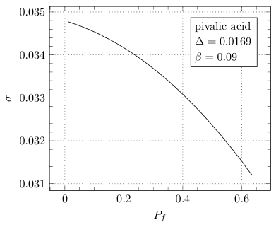
Figure 1: The stability parameter $\sigma$ as a function of the flow Péclet number $P_{f}$. Material parameters used correspond to pivalic acid with $\Delta=0.0169$ and $\beta=0.08$ dougherty91 .

Figure 1 gives the selected value of $\sigma$ as a function of the flow Péclet number for fixed undercooling $\Delta$ and an anisotropy parameter that corresponds to a measured value dougherty91 .

Figure 2: The crystal growth velocity $V$ as a function of the flow velocity $U$.

Figure 3: The tip radius of the needle crystal $\rho$ as a function of the flow velocity $U$.

In Figs. 2 and 3 we give the selected growth velocity $V$ and tip radius $\rho$ in dimensional form. We refrain from comparing these numerical results with a concrete experiment, because there are too many uncertainties regarding the applicability of the toy model to real life.

All that we wish to point out here is that there are power law scaling relations between the growth velocity and the velocity of the imposed flow as well as between the tip radius and the flow velocity, valid in a range of undercoolings. This feature will probably not disappear in a more quantitative calculation. In fact, we have checked for an extended range of anisotropies, thus varying $\sigma$ between small and very large values, that the scaling exponents change only slightly.

Finally, we do compare the values of $\rho^{2}V$ obtained from this calculation with experimental values in a flow situation bouissou89 , because $\rho^{2}V$ is expected to be a slowly varying quantity and therefore what matters mostly is the overall order of magnitude. As Fig. 4 demonstrates, this quantity compares reasonably with experiment. In fact, considering that the experimentalists describe their flow pattern as approximate Oseen flow, the agreement is not too bad. This should of course not be taken too seriously either. A real comparison will have to await a calculation with a more realistic flow (and, for pivalic acid, a different interface boundary condition).

To conclude this section, it may be noted that a local asymptotic analysis of Eq. (72) for $t\to\infty$ yields the same transcendental behavior as Eq. (61) and provides the prefactor $B_{1}$ in terms of the solution of the nonlinear equation (72) as a function of $P_{1}$ and $b$. Since the boundary condition on the tip slope was however already incorporated into the numerical scheme for the solution of Eq. (72), this calculation does not provide anything new.

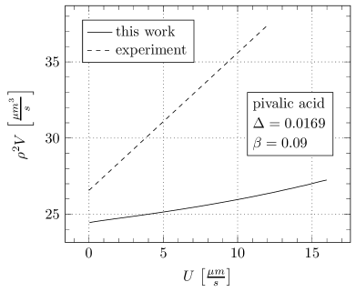
Figure 4: The product $\rho^{2}V$ as a function of the flow velocity $U$, compared with an experiment bouissou89 .

IX Conclusions

After introducing the combination of Zauderer decomposition with the Kruskal-Segur approach recently fischaleck08 ; fischaleck08b , we have now presented the method in more detail. The analytic part of the calculation has been exemplified with a fully nonlinear problem. Approximations that were introduced in fischaleck08 for didactic reasons have been removed, rendering the full power of the method visible.

We believe our approach to be the only one presented so far that has the potential of a rigorous solution of pattern selection problems with nonlinear bulk equations. Essentially, our belief that the method is rigorous rests on two facts: first, the Zauderer decomposition scheme produces a solution that becomes exact near the appropriate complex-plane singularity; second, the WKB solution derived from the interface equation within the scheme generates the same transcendental terms that a WKB solution derived from the full system of partial differential equations would. The second statement has been shown to be true for the flowless case fischaleck08b and we have given arguments here, why it should carry over to the nonlinear case as well.

The elegance and power of the method show up in its rendering the purely diffusion-limited case almost trivial fischaleck08 ; fischaleck08b . When applied to a problem with nonlinear bulk equations, calculations certainly become involved. But the problem remains solvable in a controlled manner, not provided by other methods. That in the final step the numerical determination of an eigenvalue becomes necessary should not prevent us from considering the approach basically analytical. A similar final step is necessary in almost all related problems with simpler bulk equations, even though the nonlinear equation to be solved numerically is less difficult in these cases.

We are convinced that our method will render a number of selection problems accessible to solvability theory for which controlled approximations could not be developed in the past, thus opening a new line of research. These problems would include nonlinear diffusion kurtze87 , density-driven convection sun09 (for which we have given a preliminary treatment before fischaleck02 ), Oseen flow emsellem95 ; bouissou89 , the effect of the Kapitza resistance on dendritic growth of helium franck86 ; rolley94 , but also pattern selection problems outside of crystal growth such as, for example, the motion of the two-phase front between superconducting and normal conducting parts of a material chapman95 .

Acknowledgments Financial support of this work by the German Research Foundation (DFG) under grant no. KA 672/10-1 is gratefully acknowledged.

Appendix A Conformal parabolic coordinates

The unnormalized coordinate basis is given by

$$\boldsymbol{\mathcal{E}}_{\xi}\equiv\frac{\partial\mathbf{x}}{\partial{\xi}}=\begin{pmatrix}\eta\\ -\xi\end{pmatrix}\>,\qquad\boldsymbol{\mathcal{E}}_{\eta}\equiv\frac{\partial\mathbf{x}}{\partial{\eta}}=\begin{pmatrix}\xi\\ \eta\end{pmatrix}\>,$$ (75)

which yields $g_{\xi}^{2}\equiv\left\lvert\boldsymbol{\mathcal{E}}_{\xi}\right\rvert^{2}=\xi^{2}+\eta^{2}=\left\lvert\boldsymbol{\mathcal{E}}_{\eta}\right\rvert^{2}\equiv g_{\eta}^{2}$.

Figure 5: Coordinate lines for conformal parabolic coordinates. Note that these coordinates will cover the $xy$ plane twice, if negative values for $\eta$ are admitted.

For the nabla operator, we get

$$\nabla=\frac{1}{\sqrt{\xi^{2}+\eta^{2}}}\left[\mathbf{e}_{\xi}\frac{\partial}{\partial{\xi}}+\mathbf{e}_{\eta}\frac{\partial}{\partial{\eta}}\right]\>,$$ (76)

whereas the Laplacian reads

$$\nabla^{2}=\frac{1}{\xi^{2}+\eta^{2}}\left[\frac{\partial^{2}}{\partial{\xi}^{2}}+\frac{\partial^{2}}{\partial{\eta}^{2}}\right].$$ (77)

After normalization, the basis vectors are

$$\mathbf{e}_{\xi} =\frac{1}{\sqrt{\xi^{2}+\eta^{2}}}\left(\eta\mathbf{e}_{x}-\xi\mathbf{e}_{y}\right)\>,$$ (78)

$$\mathbf{e}_{\eta} =\frac{1}{\sqrt{\xi^{2}+\eta^{2}}}\left(\xi\mathbf{e}_{x}+\eta\mathbf{e}_{y}\right)\>,$$

which can be inverted to express the Cartesian basis by the orthonormal parabolic one

$$\mathbf{e}_{x} =\frac{1}{\sqrt{\xi^{2}+\eta^{2}}}\left(\eta\mathbf{e}_{\xi}+\xi\mathbf{e}_{\eta}\right)\>,$$ (79)

$$\mathbf{e}_{y} =\frac{1}{\sqrt{\xi^{2}+\eta^{2}}}\left(\eta\mathbf{e}_{\eta}-\xi\mathbf{e}_{\xi}\right)\>.$$

Let $\eta_{s}(\xi)-\eta=0$ describe the interface, then the normal vector $\mathbf{n}$ can be derived from Frenet’s formulas. The position vector at the interface may be written

$$\mathbf{x}=\eta_{s}\xi\mathbf{e}_{x}+\frac{1}{2}\left(\eta_{s}^{2}-\xi^{2}\right)\mathbf{e}_{y}$$ (80)

and the differential line element along this curve is

$$\mathrm{d}s=\sqrt{\mathrm{d}x^{2}+\mathrm{d}y^{2}}=\sqrt{\left(\eta_{s}^{2}+\xi^{2}\right)\left(1+\eta_{s}^{\prime 2}\right)}\,\mathrm{d}\xi.$$ (81)

The tangential vector at the interface is given by $\mathrm{d}\mathbf{x}/\mathrm{d}s$, the normal vector must be orthogonal to it. By this condition, it is determined up to a sign that we choose so as to make the normal vector point into the liquid. This procedure yields

$$\mathbf{n}=\frac{1}{\sqrt{1+\eta_{s}^{\prime 2}}}\left(\mathbf{e}_{\eta}-\eta_{s}^{\prime}\mathbf{e}_{\xi}\right)\>.$$ (82)

The curvature is given by

$$\kappa =-\mathbf{n}\cdot\frac{\mathrm{d}^{2}\mathbf{r}}{\mathrm{d}{s}^{2}}$$

$$=-\frac{1}{\sqrt{\xi^{2}+\eta_{s}^{2}}}\left[\frac{\eta_{s}^{\prime\prime}}{\left(1+\eta_{s}^{\prime 2}\right)^{\frac{3}{2}}}+\frac{\eta_{s}^{\prime}\xi-\eta_{s}}{\left(\xi^{2}+\eta_{s}^{2}\right)\sqrt{1+\eta_{s}^{\prime 2}}}\right]$$ (83)

and it is positive for a convex solid.

We assume the usual model of four-fold crystalline anisotropy:

$$a(\theta)=1-\beta\cos 4\theta=1-\beta\left(1-8\cos^{2}\theta\sin^{2}\theta\right)$$ (84)

The small parameter $\beta$ is the strength of the anisotropy. $\theta$ is the angle of the interface normal with the $y$ axis, so we have $\cos\theta=\mathbf{n}\cdot\mathbf{e}_{y}$ and $\sin\theta=\mathbf{n}\cdot\mathbf{e}_{x}$, which allows us to find the anisotropy function expressed in parabolic coordinates.

$$a(\theta)=1-\beta\left[1-8\frac{\left(\xi-\eta_{s}\eta_{s}^{\prime}\right)^{2}\left(\eta_{s}+\xi\eta_{s}^{\prime}\right)^{2}}{\left(\xi^{2}+\eta_{s}^{2}\right)^{2}\left(1+\eta_{s}^{\prime 2}\right)^{2}}\right]$$ (85)

Finally, the flow velocity is given by

$$\mathbf{w}=\frac{1}{\sqrt{\xi^{2}+\eta^{2}}}\left(\psi_{\eta}\mathbf{e}_{\xi}-\psi_{\xi}\mathbf{e}_{\eta}\right)\>.$$ (86)

Appendix B Derivation of the interface equation

We first introduce some simplifications of notation. Substituting $\bar{\tau}=\xi$ and $\bar{s}^{\prime}=\frac{1}{2}(u-\xi)$ and defining

$$F(\xi) =\sigma\kappa(\xi)a(\theta(\xi))-\left(1-\mathrm{i}\xi\right)h(\xi)\>,$$ (87)

$$z(\xi) =1+\mathrm{i}h^{\prime}(\xi)\>,$$ (88)

$$\bar{z}(\xi) =1-\mathrm{i}h^{\prime}(\xi)\>,$$ (89)

we have from Eq. (57) with (58)

$$F^{\prime}(\xi) =-\frac{\mathrm{i}}{2}P_{f}\xi\bar{z}(\xi)\int\limits_{\xi}^{\mathrm{i}\infty}M\left(\frac{1}{2}(\xi-u),u\right)\mathrm{d}u$$

$$-\frac{1}{2}P_{f}\bar{z}(\xi)\int\limits_{\xi}^{\mathrm{i}\infty}\frac{\left[uh\right]^{\prime}}{z(u)}\mathrm{e}^{\frac{P_{f}}{8}\left(\xi-u\right)^{2}}\mathrm{d}u$$ (90)

with the prime denoting a derivative with respect to $\xi$ or $u$, depending on whether the term concerned is outside or inside an integral. Writing out $M$, we have

$$M\left(\frac{1}{2}(\xi-u),u\right)=\frac{\mathrm{i}}{2z(u)}\mathrm{e}^{\frac{P_{f}}{8}\left(\xi^{2}-u^{2}\right)}$$

$$\hskip 14.22636pt\times\left[\left[\left(1+\mathrm{i}u\right)h\right]^{\prime}-\frac{2\left[uh\right]^{\prime}}{u}\left(1-\mathrm{e}^{-\frac{P_{f}}{4}\left(\xi-u\right)u}\right)\right]$$ (91)

and

$$\frac{\partial}{\partial{\xi}}M\left(\frac{1}{2}(\xi-u),u\right) =\frac{P_{f}\xi}{4}M\left(\frac{1}{2}(\xi-u),u\right)$$

$$\;\;-\frac{\mathrm{i}P_{f}}{4}\frac{\left[uh\right]^{\prime}}{z(u)}\mathrm{e}^{\frac{P_{f}}{8}\left(\xi-u\right)^{2}}.$$ (92)

Inserting this into (90), we obtain a useful expression for the derivative of $F$:

$$F^{\prime}(\xi) =-2\mathrm{i}\bar{z}(\xi)\int\limits_{\xi}^{\mathrm{i}\infty}\frac{\partial}{\partial{\xi}}M\left(\frac{1}{2}(\xi-u),u\right)\mathrm{d}u$$

$$=-2\mathrm{i}\bar{z}(\xi)\left[\frac{\partial}{\partial{\xi}}\int\limits_{\xi}^{\mathrm{i}\infty}M\left(\frac{1}{2}(\xi-u),u\right)\mathrm{d}u+M(0,\xi)\right]$$

$$=-2\mathrm{i}\bar{z}(\xi)\frac{\partial}{\partial{\xi}}\int\limits_{\xi}^{\mathrm{i}\infty}M\left(\frac{1}{2}(\xi-u),u\right)\mathrm{d}u$$

$$\hskip 14.22636pt+\frac{\bar{z}(\xi)}{z(\xi)}\left[\left(1+\mathrm{i}\xi\right)h(\xi)\right]^{\prime}.$$ (93)

This can be integrated by parts. Using

$$\left[\frac{\bar{z}}{z}\right]^{\prime}=-2\mathrm{i}\frac{h^{\prime\prime}}{z^{2}}\>,$$ (94)

we arrive at

$$F(\xi)= -2\mathrm{i}\bar{z}(\xi)\int\limits_{\xi}^{\mathrm{i}\infty}M\left(\frac{1}{2}(\xi-u),u\right)\mathrm{d}u$$

$$+2\int\limits^{\xi}h^{\prime\prime}(\xi^{\prime})\int\limits_{\xi^{\prime}}^{\mathrm{i}\infty}M\left(\frac{1}{2}(\xi^{\prime}-u),u\right)\mathrm{d}u\,\mathrm{d}\xi^{\prime}$$

$$+\frac{\bar{z}(\xi)}{z(\xi)}\left(1+\mathrm{i}\xi\right)h(\xi)$$

$$+2\mathrm{i}\int\limits^{\xi}\frac{h^{\prime\prime}(\xi^{\prime})}{z^{2}(\xi^{\prime})}\left(1+\mathrm{i}\xi^{\prime}\right)h(\xi^{\prime})\mathrm{d}\xi^{\prime}\>,$$ (95)

which is not quite the form we want. On the one hand, equation (95) manifests a certain generality, since it is valid for arbitrary flows. But on the other hand, we would appreciate to have a right hand side that obviously vanishes for $P_{f}\to 0$. To achieve this, we use (95) to eliminate the first term on the right hand side of (90):

$$F^{\prime}(\xi)= \frac{P_{f}}{4}\xi F(\xi)-\frac{P_{f}}{4}\xi\frac{\bar{z}(\xi)}{z(\xi)}\left(1+\mathrm{i}\xi\right)h(\xi)$$

$$-\frac{\mathrm{i}}{2}P_{f}\xi\int\limits^{\xi}\frac{h^{\prime\prime}(\xi^{\prime})}{z^{2}(\xi^{\prime})}\left(1+\mathrm{i}\xi^{\prime}\right)h(\xi^{\prime})\mathrm{d}\xi^{\prime}$$

$$-\frac{P_{f}}{2}\xi\int\limits^{\xi}h^{\prime\prime}(\xi^{\prime})\int\limits_{\xi^{\prime}}^{\mathrm{i}\infty}M\left(\frac{1}{2}(\xi^{\prime}-u),u\right)\mathrm{d}u\,\mathrm{d}\xi^{\prime}$$

$$-\frac{P_{f}}{2}\bar{z}(\xi)\int\limits_{\xi}^{\mathrm{i}\infty}\frac{\left[uh\right]^{\prime}}{z(u)}\mathrm{e}^{\frac{P_{f}}{8}\left(\xi-u\right)^{2}}\mathrm{d}u$$ (96)

Employing the identities

$$\int\limits_{\xi}^{\mathrm{i}\infty}\frac{\left[uh\right]^{\prime}}{z(u)}\mathrm{e}^{\frac{P_{f}}{8}\left(\xi-u\right)^{2}}\mathrm{d}u =-\frac{\xi h(\xi)}{z(\xi)}$$

$$-\int\limits_{\xi}^{\mathrm{i}\infty}\left[uh(u)\left(\frac{\left(u-\xi\right)P_{f}}{4z(u)}-\frac{\mathrm{i}h^{\prime\prime}(u)}{z^{2}(u)}\right)\mathrm{e}^{\frac{P_{f}}{8}\left(\xi-u\right)^{2}}\right]\mathrm{d}u\>,$$ (97)

$$F^{\prime}(\xi)-\frac{P_{f}}{4}\xi F(\xi) =\mathrm{e}^{\frac{P_{f}}{8}\xi^{2}}\frac{\mathrm{d}}{\mathrm{d}{\xi}}\left[F(\xi)\mathrm{e}^{-\frac{P_{f}}{8}\xi^{2}}\right]\>,$$ (98)

the first of which is obtained via integration by parts again, we may rewrite (96) as follows

$$\mathrm{e}^{\frac{P_{f}}{8}\xi^{2}} \frac{\mathrm{d}}{\mathrm{d}{\xi}}\left[F(\xi)\mathrm{e}^{-\frac{P_{f}}{8}\xi^{2}}\right]=\,\frac{P_{f}}{4}\frac{\bar{z}(\xi)}{z(\xi)}\xi\left(1-\mathrm{i}\xi\right)h(\xi)$$

$$+\frac{P_{f}}{2}\bar{z}(\xi)\int\limits_{\xi}^{\mathrm{i}\infty}\left[\rule{0.0pt}{17.07164pt}\right.uh(u)\left(\rule{0.0pt}{12.80373pt}\right.\frac{\left(u-\xi\right)P_{f}}{4z(u)}$$

$$\hskip 56.9055pt-\frac{\mathrm{i}h^{\prime\prime}(u)}{z^{2}(u)}\left.\rule{0.0pt}{12.51918pt}\right)\mathrm{e}^{\frac{P_{f}}{8}\left(\xi-u\right)^{2}}\left.\rule{0.0pt}{17.07164pt}\right]\mathrm{d}u$$

$$-\frac{\mathrm{i}}{2}P_{f}\xi\int\limits^{\xi}\frac{h^{\prime\prime}(\xi^{\prime})}{z^{2}(\xi^{\prime})}\left(1+\mathrm{i}\xi^{\prime}\right)h(\xi^{\prime})\mathrm{d}\xi^{\prime}$$

$$-\frac{P_{f}}{2}\xi\int\limits^{\xi}h^{\prime\prime}(\xi^{\prime})\int\limits_{\xi^{\prime}}^{\mathrm{i}\infty}M\left(\frac{1}{2}(\xi^{\prime}-u),u\right)\mathrm{d}u\,\mathrm{d}\xi^{\prime}.$$ (99)

With one further integration, we arrive at Eq. (59).

References

- (1) J. Kepler, “Strena seu de nive sexangula,” G. Tampach, editor, Frankfurt (1611), A New Year’s Gift or on the Six-Cornered Snowflake. Editor and Trans. C. Hardie (Oxford at the Clarendon Press, Oxford, 1966) p. 74
- (2) Linear systems may display interesting patterns due to boundary conditions. Chladni figures are a well-known example. However, we rather speak of pattern formation, when scale selection is intrinsic to the dynamics.
- (3) G. P. Ivantsov, Dokl. Akad. Naut. SSSR 58, 567 (1947)
- (4) J. Langer, Phys. Rev. A 33, 435 (1986)
- (5) B. Caroli, C. Caroli, B. Roulet, and J. Langer, Phys. Rev. A 33, 442 (1986)
- (6) M. B. Amar and Y. Pomeau, Europhys. Lett. 2, 307 (1986)
- (7) E. Ben-Jacob, N. Goldenfeld, B. G. Kotliar, and J. S. Langer, Phys. Rev. Lett. 53, 2110 (1984)
- (8) D. Kessler, J. Koplik, and H. Levine, Phys. Rev. A 31, 1712 (1985)
- (9) What is said here for surface tension, holds, mutatis mutandis, also for interfacial kinetics. With an anisotropic term for the velocitity-dependent deviation of the interface temperature from its equilibrium value, selection happens even if the Gibbs-Thomson effect is not taken into account brener91 . If both surface tension and the kinetic term are isotropic, there is no selection of parabolic shapes in free growth.
- (10) D. C. Hong and J. S. Langer, Phys. Rev. Lett. 56, 2032 (1986)
- (11) B. I. Shraiman, Phys. Rev. Lett. 56, 2028 (1986)
- (12) R. Combescot, T. Dombre, V. Hakim, Y. Pomeau, and A. Pumir, Phys. Rev. Lett. 56, 2036 (1986)
- (13) D. I. Meiron, Phys. Rev. A 33, 2704 (1986)
- (14) D. A. Kessler, J. Koplik, and H. Levine, Phys. Rev. A 33, 3352 (1986)
- (15) D. A. Kessler and H. Levine, Phys. Rev. B 33, 7867 (1986)
- (16) A. Barbieri, D. C. Hong, and J. S. Langer, Phys. Rev. A 35, 1802 (1987)
- (17) D. A. Kessler and H. Levine, Phys. Rev. A 36, 4123 (1987)
- (18) D. A. Kessler and H. Levine, Acta Metall. 36, 2693 (1988)
- (19) M. B. Amar and E. Brener, Phys. Rev. Lett. 71, 589 (1993)
- (20) E. Brener, Phys. Rev. Lett. 71, 3653 (1993)
- (21) J. S. Langer, Phys. Rev. A 33, 435 (1986)
- (22) M. D. Kruskal and H. Segur, Stud. Appl. Math. 85, 129 (1991), this paper has been often quoted as A.R.A.P. Tech. Memo 25, 1985
- (23) S. Tanveer, Phys. Rev. A 40, 4756 (1989)
- (24) M. B. Amar, Phys. Rev. A 41, 2080 (1990)
- (25) E. Brener and V. Mel′nikov, Advances in Physics 40, 53 (1991)
- (26) S. Tanveer, J. Fluid Mech. 409, 273 (2000)
- (27) D. C. Hong and J. S. Langer, Phys. Rev. A 36, 2325 (1987)
- (28) A. Barbieri and J. S. Langer, Phys. Rev. A 39, 5314 (1989)
- (29) P. Bouissou and P. Pelcé, Phys. Rev. A 40, 6673 (1989)
- (30) P. Pelcé, Dynamics of curved Fronts (Academic Press, Boston, 1988)
- (31) D. Alexandrov, P. Galenko, and D. Herlach, J. Cryst. Growth 312, 2122 (2010)
- (32) T. Fischaleck and K. Kassner, EPL 81, 54004 (2008)
- (33) T. Fischaleck, An Approach to Selection Theory for Dendritic Growth Enabling the Treatment of General Bulk Equations, Ph.D. thesis, Otto-von-Guericke Universität (2008)
- (34) E. Zauderer, SIAM J. Appl. Math. 35, 575 (1978)
- (35) D. Saville and P. Beaghton, Phys. Rev. A 37, 3423 (1988)
- (36) P. Nozières, “Shape and growth of crystals,” in Solids far from Equilibrium, edited by C. Godrèche (Cambridge University Press, Cambridge, 1992) pp. 1–154
- (37) Meaning that no volume element of the solid is in motion. The interface moves, of course, due to the addition of solid.
- (38) S. K. Dash and W. N. Gill, Int. J. Heat Mass Transfer 27, 1345 (1984)
- (39) M. Ben Amar, P. Bouissou, and P. Pelcé, J. Cryst. Growth 92, 97 (1988)
- (40) L. Cummings, Y. Hohlov, S. Howison, and K. Kornev, J. Fluid Mech. 378, 1 (1999)
- (41) C. M. Bender and S. A. Orszag, Advanced Mathematical Methods for Scientists and Engineers (McGraw-Hill, New York, 1978)
- (42) As we shall see later, we do not precisely expand about the flow-Ivantsov solution but rather about an approximation to it that becomes accurate in the vicinity of the appropriate complex-plane singularity.
- (43) The argument to obtained by setting and can alternatively be constructed setting and .
- (44) Actually, what is important is not that the solution remains a good approximation near the interface but only that it captures the transcendental term which in regular perturbation theory lies beyond all orders.
- (45) In the form we employ, the method is not suited for Dirichlet boundary conditions, due to the transformation to a first-order system.
- (46) Note that the curvature vanishes for and becomes equal to the curvature of the Ivantsov parabola for , hence vanishes for in that case.
- (47) It should be kept in mind that the variable introduced here has nothing to do with a time. Nevertheless, we denote derivatives with respect to by overdots.
- (48) R. Ananth and W. N. Gill, J. Cryst. Growth 108, 173 (1990)
- (49) Since our calculation is valid for , we may also, for finite , use the analytic approximation obtained by setting on the right-hand side of Eq. (27\@@italiccorr), without changing the order in up to which the calculation is correct; in the case of , we first have to evaluate the integral on the right-hand side, but still may set in the exponential prefactor. The numerical evaluation of interpolates smoothly between these two limits, corresponding to and , respectively.
- (50) A potential flow would be expected around solid helium growing into its superfluid. For such a system, the Gibbs-Thomson condition will not describe the interface temperature correctly anymore due to the appearance of a Kapitza resistance. Moreover, the only experiments on dendritic growth with solid helium we are aware of franck86 ; rolley94 (4He, 3He) were done at temperatures well above the transition to superfluidity.
- (51) C. Misbah, J. Phys. France 48, 1265 (1987)
- (52) M. Muschol, D. Liu, and H. Z. Cummins, Phys. Rev. A 46, 1038 (1992)
- (53) P. Bouissou, B. Perrin, and P. Tabeling, Phys. Rev. A 40, 509 (1989)
- (54) Y.-W. Lee, R. Ananth, and W. N. Gill, J. Cryst. Growth 132, 226 (1993)
- (55) E. Rubinstein and M. Glicksman, J. Crystal Growth 112, 84 (1991)
- (56) A. Dougherty, J. Cryst. Growth 110, 501 (1991)
- (57) This is not the radius of curvature at the tip of the true crystal but the one corresponding to a flow-Ivantsov solution traveling at the same velocity, i.e., the radius should be obtained by fitting the tail of an experimental needle crystal – after removal of noise-induced side branches – to a parabola. Since correction for side branches is tricky, one may instead fit to an appropriate piece of the needle crystal ahead of the side-branching region but not too close to the tip.
- (58) D. A. Kurtze, Phys. Rev. A 36, 232 (1987)
- (59) Y. Sun and C. Beckerman, J. Cryst. Growth 311, 4447 (2009)
- (60) T. Fischaleck and K. Kassner, Verh. DPG 37, 128 (2002), DY46.68
- (61) V. Emsellem and P. Tabeling, J. Cryst. Growth 156, 285 (1995)
- (62) J. P. Franck and J. Jung, J. Low Temp. Phys. 64, 165 (1986)
- (63) G. Rolley, S. Balibar, and F. Graner, Phys. Rev. E 49, 1500 (1994)
- (64) S. J. Chapman, in Proceedings of the first world congress on World congress of nonlinear analysts ’92, volume IV, WCNA ’92 (Walter de Gruyter & Co., Hawthorne, NJ, USA, 1995) pp. 3803–3809