Uniform electron gases. I. Electrons on a ring

Abstract

We introduce a new paradigm for one-dimensional uniform electron gases (UEGs). In this model, $n$ electrons are confined to a ring and interact via a bare Coulomb operator. We use Rayleigh-Schrödinger perturbation theory to show that, in the high-density regime, the ground-state reduced (i.e. per electron) energy can be expanded as $\epsilon(r_{s},n)=\epsilon_{0}(n)r_{s}^{-2}+\epsilon_{1}(n)r_{s}^{-1}+\epsilon_{2}(n)+\epsilon_{3}(n)r_{s}+\ldots$, where $r_{s}$ is the Seitz radius. We use strong-coupling perturbation theory and show that, in the low-density regime, the reduced energy can be expanded as $\epsilon(r_{s},n)=\eta_{0}(n)r_{s}^{-1}+\eta_{1}(n)r_{s}^{-3/2}+\eta_{2}(n)r_{s}^{-2}+\ldots$. We report explicit expressions for $\epsilon_{0}(n)$, $\epsilon_{1}(n)$, $\epsilon_{2}(n)$, $\epsilon_{3}(n)$, $\eta_{0}(n)$ and $\eta_{1}(n)$ and derive the thermodynamic (large-$n$) limits of each of these. Finally, we perform numerical studies of UEGs with $n=2,3,\ldots,10$, using Hylleraas-type and quantum Monte Carlo methods, and combine these with the perturbative results to obtain a picture of the behavior of the new model over the full range of $n$ and $r_{s}$ values.

I Introduction

In a recent paper, Gill and Loos (2012) we showed that the traditional concept of the uniform electron gas (UEG), i.e. a homogeneous system of finite density, consisting of an infinite number of electrons in an infinite volume, Giuliani and Vignale (2005); Loos and Gill (2011a, b) is inadequate to model the UEGs that arise in finite systems. Accordingly, we proposed to embark on a comprehensive study of quasi-exact properties of finite-size UEGs, in order eventually to create improved approximations in density-functional theory. Parr and Yang (1989)

In an earlier paper, Loos and Gill (2011c) we introduced an alternative paradigm, in which $n$ electrons are confined to a $D$-sphere (with $D\geq 2$), that is, the surface of a ($D+1$)-dimensional ball. These systems possess uniform densities, even for finite $n$ and, because all points on a $D$-sphere are equivalent, their mathematical analysis is relatively straightforward. Loos and Gill (2009a, b, 2010a); Loos (2010); Loos and Gill (2010b); Loos (2012) In the present paper, we study the one-dimensional ($D=1$) version of model, in which $n$ electrons are confined to a ring of radius $R$. The electron density of this $n$-electron UEG, which we will call $n$-ringium, is

$$\rho=\frac{n}{2\pi R}=\frac{1}{2\,r_{s}},$$ (1)

where $r_{s}=\pi R/n$ is the Seitz radius. In this study, the high-density (small-$r_{s}$) limit is defined by $R\to 0$ for fixed $n$, while the low-density (large-$r_{s}$) limit is defined by $R\to\infty$ for fixed $n$. We do not include a fictitious uniform positive background charge because, unlike the situation in 2D and 3D UEGs, its inclusion in 1D systems causes the Coulomb energy to diverge.

In most previous work on the one-dimensional (1D) UEG, the true Coulomb potential $1/r_{12}$ has been avoided because of the intractability of its Fourier transform. Instead, most workers have softened the potential, either by adding a transverse harmonic component Pederiva and Lipparini (2002); Casula, Sorella, and Senatore (2006); Lee and Drummond (2011) or by using a potential of the form $1/\sqrt{r_{12}^{2}+\mu^{2}}$. In the latter case, the $\mu$ parameter eliminates the singularity at $r_{12}=0$ while retaining the long-range Coulomb tail. Schulz (1993); Fogler (2005); Lee and Drummond (2011)

However, the introduction of a parameter $\mu>0$ is undesirable, for it modifies the physics of the system in the high-density regime where neighboring electrons repel far too weakly. It is also unnecessary, because the true Coulomb potential is so repulsive that it causes the wave function to vanish when any two electrons touch, thereby removing the possibility of an energy divergence. Astrakharchik and Girardeau (2011) For 1D systems, we have recently shown that the exact wave function $\Psi$ behaves as

$$\Psi(r_{12})=r_{12}\left(1+\frac{r_{12}}{2}\right)+O(r_{12}^{3})$$ (2)

for small $r_{12}$, Loos and Gill (2012) which is the 1D analog of the (three-dimensional) Kato cusp condition. Kato (1957)

This nodal behavior leads to the 1D Bose-Fermi mapping Girardeau (1960) which states that the ground state wave function of the bosonic (B) and fermionic (F) states are related by $\Psi_{\text{B}}(\mathbf{R})=\left|\Psi_{\text{F}}(\mathbf{R})\right|$, where $\mathbf{R}=(\mathbf{r}_{1},\mathbf{r}_{2},\ldots,\mathbf{r}_{n})$ are the one-particle coordinates. In case of bosons, the divergence of the Coulomb potential has the effect of mimicking the Pauli principle which prohibits two fermions from touching. This implies that, for 1D systems, the bosonic and fermionic ground states are degenerate and the system is “spin-blind”. Consequently, the paramagnetic and ferromagnetic states are degenerate and we will consider only the latter. Lee and Drummond (2011)

The electrons-on-a-ring paradigm has been intensively studied as a model for quantum rings (QRs), which are tiny, self-organised, ring-shaped semiconductors Warburton et al. (2000); Fuhrer et al. (2001) characterised by three parameters: radius ($R$), width ($\delta$) and electron number ($n$). Modern microfabrication technology has yielded InGaAs and GaAlAs/GaAs QRs that bind only a few electrons, Lorke et al. (2000); Keyser et al. (2003) in contrast with the mesoscopic rings on GaAs which hold much larger numbers of electrons. Mailly, Chapelier, and Benoit (1993) These low-dimensional systems are the subject of considerable scientific interest and have been intensively studied, both experimentally Mailly, Chapelier, and Benoit (1993); Warburton et al. (2000); Lorke et al. (2000); Fuhrer et al. (2001); Bayer et al. (2003); Keyser et al. (2003); Fuhrer et al. (2004); Sigrist et al. (2004) and theoretically, Viefers et al. (2004); Fogler and Pivovarov (2005, 2006); Niemela et al. (1996); Gylfadottir et al. (2006); Pederiva and Lipparini (2002); Emperador, Pederiva, and Lipparini (2003); Emperador et al. (2001); Räsänen et al. (2009); Aichinger et al. (2006); Manninen and Reimann (2009); Loos and Gill (2012) mainly because of the observation of Aharonov-Bohm oscillations. Aharonov and Bohm (1959); Aronov and Lyanda-Geller (1993); Morpurgo et al. (1998); Emperador, Pederiva, and Lipparini (2003)

As a first approximation, QRs can be modelled by electrons confined to a perfect ring (i.e. $\delta=0$). In a recent paper, Loos and Gill (2012) we considered a pair of electrons (i.e. $n=2$) on such a ring and discovered that their Schrödinger equation can be solved exactly, provided that the radius takes one of an infinite number of special values. Some of the solutions exhibit the Berry phase phenomenon, i.e. if one of the electrons moves once around the ring and returns to its starting point, the wave function of the system changes sign. QRs are among the simplest systems with this peculiar property.

In Section II, we first use Rayleigh-Schrödinger perturbation theory to investigate the energy in the high-density regime Gell-Mann and Brueckner (1957) and then strong-coupling perturbation theory to study the low-density regime, where the electrons form a Wigner crystal. Wigner (1934) In Section III, we use explicitly correlated (EC) methods to determine the energy of $n$-ringium for $n=2,3,4,5$. These methods are accurate for very small $n$ but their cost grows very rapidly with $n$. In Section IV, we turn to quantum Monte Carlo (QMC) approaches for studying $n$-ringium up to $n=10$ over a range of densities. These methods provide a different approach to the many-body problem: variational Monte Carlo (VMC) McMillan (1965); Ceperley, Chester, and Kalos (1977); Umrigar (1999) and diffusion Monte Carlo (DMC) Kalos, Levesque, and Verlet (1974); Ceperley and Kalos (1979); Reynolds et al. (1982) methods can be used to treat systems in one and higher dimensions at a computational cost that grows relatively slowly with $n$ (at least, when $n$ is not too large. Nemec (2010))

We frame our discussion in terms of reduced energy $\epsilon(r_{s},n)$, i.e. energy per electron, so that we can pass smoothly from finite to infinite $n$. One of the key goals of the paper is to develop an understanding of the correlation energy, which is defined as the difference

$$\epsilon_{\rm c}(r_{s},n)=\epsilon(r_{s},n)-\epsilon_{\rm HF}(r_{s},n),$$ (3)

between the exact and Hartree-Fock (HF) energies. Atomic units are used throughout, but we report total energies in hartrees ($E_{\rm h}$) and correlation energies in millihartrees (${\rm m}E_{\rm h}$).

II Perturbative methods

II.1 High-density expansion

The Hamiltonian of the system is

$$H=-\frac{1}{2R^{2}}\sum_{i=1}^{n}\frac{\partial^{2}}{\partial\theta_{i}^{2}}+\sum_{i<j}^{n}\frac{1}{r_{ij}},$$ (4)

where $\theta_{i}$ is the angle of electron $i$ around the ring center, and

$$r_{ij}=\left|\mathbf{r}_{i}-\mathbf{r}_{j}\right|=R\sqrt{2-2\cos(\theta_{i}-\theta_{j})}$$ (5)

is the across-the-ring distance between electrons $i$ and $j$.

In the high-density (i.e. small $r_{s}$) regime, the kinetic energy is dominant and it is natural to define a zeroth-order Hamiltonian

$$H_{0}=-\frac{1}{2R^{2}}\sum_{i=1}^{n}\frac{\partial^{2}}{\partial\theta_{i}^{2}},$$ (6)

and a perturbation

$$V=\sum_{i<j}^{n}r_{ij}^{-1}.$$ (7)

The non-interacting orbitals and orbital energies are

$$\chi_{a}(\theta)=(2\pi R)^{-1/2}\exp(i\,a\,\theta),$$ (8)

$$\kappa_{a}=\frac{a^{2}}{2R^{2}},$$ (9)

where

$$a=\begin{cases}\ldots,-2,-1,0,+1,+2,\ldots,&\text{if $n$ is odd,}\\ \ldots,-\frac{3}{2},-\frac{1}{2},+\frac{1}{2},+\frac{3}{2},\ldots,&\text{if $n$ is even.}\end{cases}$$ (10)

A Slater determinant ${}^{n}\Psi_{i}$ of any $n$ of these orbitals has an energy $E_{i}$ and is an antisymmetric eigenfunction of $H_{0}$. In the lowest energy (aufbau) determinant ${}^{n}\Psi_{0}$, we occupy the orbitals with

$$a=-\frac{n-1}{2},-\frac{n-3}{2},\ldots,+\frac{n-3}{2},+\frac{n-1}{2}.$$ (11)

Following the approach of Mitas, Mitas (2006) one discovers the remarkable result

$$^{n}\Psi_{0}\propto\prod_{i<j}^{n}\hat{r}_{ij},$$ (12)

where

$$\hat{r}_{ij}=2R\sin\left(\frac{\theta_{i}-\theta_{j}}{2}\right)$$ (13)

is a signed interelectronic distance. It follows immediately that ${}^{n}\Psi_{0}$ has a node whenever $\theta_{i}=\theta_{j}$ and, therefore, possesses the same nodes as the exact wave function. This will have important ramifications in Section IV.

Rayleigh-Schrödinger theory yields the perturbation expansion for the reduced energy

$$\epsilon(r_{s},n)=\frac{\epsilon_{0}(n)}{r_{s}^{2}}+\frac{\epsilon_{1}(n)}{r_{s}}+\epsilon_{2}(n)+\epsilon_{3}(n)r_{s}+\ldots,$$ (14)

where the high-density coefficients $\epsilon_{j}(n)$ are found by setting $R=1$ and evaluating

$$\epsilon_{0}(n) =\frac{\pi^{2}}{n^{3}}\langle\Psi_{0}|H_{0}|\Psi_{0}\rangle,$$ (15a)

$$\epsilon_{1}(n) =\frac{\pi}{n^{2}}\langle\Psi_{0}|V|\Psi_{0}\rangle,$$ (15b)

$$\epsilon_{2}(n) =\frac{1}{n}\sum_{i}\frac{\langle\Psi_{0}|V|\Psi_{i}\rangle\langle\Psi_{i}|V|\Psi_{0}\rangle}{E_{0}-E_{i}},$$ (15c)

$$\epsilon_{3}(n) =\frac{1}{\pi}\sum_{i}\sum_{j}\frac{\langle\Psi_{0}|V|\Psi_{i}\rangle\langle\Psi_{i}|V-n^{2}\epsilon_{1}/\pi|\Psi_{j}\rangle\langle\Psi_{j}|V|\Psi_{0}\rangle}{(E_{0}-E_{i})(E_{0}-E_{j})}.$$ (15d)

II.1.1 Double-bar integrals

To evaluate the coefficients $\epsilon_{j}(n)$ with $j>0$, one requires the “double-bar” integrals

$$\langle ab||cd\rangle=\int_{0}^{2\pi}\!\!\!\int_{0}^{2\pi}\frac{\chi_{a}^{*}(\theta_{1})\chi_{b}^{*}(\theta_{2})[\chi_{c}(\theta_{1})\chi_{d}(\theta_{2})-\chi_{c}(\theta_{2})\chi_{d}(\theta_{1})]}{r_{12}}d\theta_{1}d\theta_{2}.$$ (16)

By elementary integration, one can show that

$$\langle ab||cd\rangle=\begin{cases}V_{c-b,c-a},&a+b=c+d,\\ \qquad 0,&\text{otherwise,}\end{cases}$$ (17)

where

$$V_{p,q}=\frac{1}{\pi}\left[\psi(p+\tfrac{1}{2})-\psi(q+\tfrac{1}{2})\right],$$ (18)

and $\psi$ is the digamma function. Olver et al. (2010)

Table 1: High-density coefficients for $n$-ringium. ($\zeta(3)$ is Apéry’s constant. Olver et al. (2010))

$n$	$\epsilon_{0}(n)$	$\epsilon_{1}(n)$	$\epsilon_{2}(n)$	$\epsilon_{3}(n)$
2	$\frac{1}{32}\pi^{2}$	$\frac{1}{2}$	$1-\frac{10}{\pi^{2}}$	$\frac{8(12\ln 2-19)}{3\pi^{2}}+\frac{16(26-7\zeta(3))}{\pi^{4}}$
3	$\frac{1}{27}\pi^{2}$	$\frac{20}{27}$	$\frac{16}{9}-\frac{1436}{81\pi^{2}}$	$\frac{8(1080\ln 2-997)}{81\pi^{2}}+\frac{8(13046-4725\zeta(3))}{243\pi^{4}}$
4	$\frac{5}{128}\pi^{2}$	$\frac{9}{10}$	$\frac{109}{45}-\frac{244168}{10125\pi^{2}}$	0.00487354
5	$\frac{1}{25}\pi^{2}$	$\frac{892}{875}$	$\frac{4688}{1575}-\frac{514012364}{17364375\pi^{2}}$	0.00556461
6	$\frac{35}{864}\pi^{2}$	$\frac{6323}{5670}$	$\frac{2339}{675}-\frac{461265158}{13395375\pi^{2}}$	0.00605813
7	$\frac{2}{49}\pi^{2}$	$\frac{13528}{11319}$	$\frac{1420256}{363825}-\frac{33870168846728}{873632962125\pi^{2}}$	0.00642454
8	$\frac{21}{512}\pi^{2}$	$\frac{7591}{6006}$	$\frac{20349053}{4729725}-\frac{81975019672689056}{1919371617788625\pi^{2}}$	0.00670533
9	$\frac{10}{243}\pi^{2}$	$\frac{4831544}{3648645}$	$\frac{66244064}{14189175}-\frac{266761139809046216}{5758114853365875\pi^{2}}$	0.00692616
10	$\frac{33}{800}\pi^{2}$	$\frac{2512297}{1823250}$	$\frac{1207979879}{241215975}-\frac{7026989855398034506022}{141448091372932719375\pi^{2}}$	0.00710359
$\infty$	$\pi^{2}/24$	$\ln\sqrt{n}$	$-\pi^{2}/360$	$0.00844621$

II.1.2 Zeroth order

The zeroth-order coefficient (15a) becomes

$$\epsilon_{0}(n)=\frac{\pi^{2}}{n^{3}}\sum_{a}^{\text{occ}}\frac{a^{2}}{2},$$ (19)

where the “occ” indicates sums over all occupied orbitals (11), and this reduces to

$$\epsilon_{0}(n)=\frac{n^{2}-1}{n^{2}}\frac{\pi^{2}}{24}.$$ (20)

In the thermodynamic (i.e. $n\to\infty$) limit, this approaches

$$\epsilon_{0}=\frac{\pi^{2}}{24},$$ (21)

which is identical to the kinetic energy coefficient in the ideal Fermi gas in 1D. Giuliani and Vignale (2005); Loos and Gill (2011c)

II.1.3 First order

The first-order coefficient (15b) becomes

$$\epsilon_{1}(n)=\frac{\pi}{n^{2}}\sum_{a<b}^{\text{occ}}\langle ab||ab\rangle,$$ (22)

which can be reduced to

$$\epsilon_{1}(n)=\left(\frac{1}{2}-\frac{1}{8n^{2}}\right)\left[\psi(n+\tfrac{1}{2})-\psi(\tfrac{1}{2})\right]-\frac{3}{4}.$$ (23)

This can be found in closed form for any $n$ (see Table 1). Because of the slow decay of the Coulomb operator, the coefficient grows logarithmically with $n$ and it can be shown that

$$\epsilon_{1}(n)\sim\ln\sqrt{n}+(\ln 2+\gamma/2-3/4)+O(n^{-2}\ln n),$$ (24)

where $\gamma$ is the Euler-Mascheroni constant. Olver et al. (2010)

The sum of the first two terms in (14) gives the HF energy of $n$-ringium

$$\epsilon_{\text{HF}}(r_{s},n)=\frac{\epsilon_{0}(n)}{r_{s}^{2}}+\frac{\epsilon_{1}(n)}{r_{s}}.$$ (25)

II.1.4 Second order

The second-order coefficient (15c) becomes

$$\epsilon_{2}(n)=-\frac{1}{n}\sum_{a<b}^{\text{occ}}\sum_{r<s}^{\text{virt}}\frac{\langle ab||rs\rangle\langle rs||ab\rangle}{\kappa_{r}+\kappa_{s}-\kappa_{a}-\kappa_{b}},$$ (26)

where the “virt” indicates sums over all virtual orbitals. If the double-bar integrals do not vanish, i.e. $a+b=r+s$, then

$$\kappa_{r}+\kappa_{s}-\kappa_{a}-\kappa_{b}=(r-a)(r-b),$$ (27)

and we obtain

$$\epsilon_{2}(n)=-\frac{1}{n}\sum_{a<b}^{\text{occ}}\sum_{r=r_{\text{min}}}^{\infty}\frac{V_{r-a,r-b}^{2}}{(r-a)(r-b)},$$ (28)

where

$$r_{\text{min}}=\frac{n+1}{2}+\max(a+b,0).$$ (29)

The sums in (28) can be evaluated in closed form for any $n$ (see Table 1). In the $r_{s}\to 0$ limit, the higher terms in (14) vanish and the $\epsilon_{2}(n)$ expressions in Table 1 are therefore the exact correlation energies of infinitely dense $n$-ringium.

In the thermodynamic limit, $\epsilon_{2}(n)$ approaches

$$\epsilon_{2} =-\lim_{n\to\infty}\frac{1}{n}\sum_{a<b}^{\text{occ}}\sum_{r=r_{\text{min}}}^{\infty}\frac{\left[\frac{1}{\pi}\ln\left(\frac{r-a}{r-b}\right)\right]^{2}}{(r-a)(r-b)}$$

$$=-\frac{1}{3\pi^{2}}\int_{0}^{1}\!\!\int_{-x}^{x}\frac{1}{x-y}\ln^{3}\left(\frac{1+x}{1+y}\right)\,dx\,dy$$

$$=-\frac{\pi^{2}}{360},$$ (30)

which implies that, in the dual thermodynamic/high-density limit, the exact correlation energy of ringium is $-27.4\ {\rm m}E_{\rm h}$ per electron. The same value of $\epsilon_{2}$ can be derived for 1D jellium, Loos (2013) affirming the equivalence of the electrons-on-a-ring and electrons-on-a-wire models in the thermodynamic limit. Loos and Gill (2011c)

Using a quasi-1D model with a transverse harmonic potential, Casula et al. were led to conclude that, in the same limit, the correlation energy vanishes. Casula, Sorella, and Senatore (2006) This qualitatively different prediction stresses the importance of employing a realistic Coulomb operator for high-density UEGs.

II.1.5 Third order

The third-order coefficient (15d) becomes

$$\epsilon_{3}(n) =\frac{1}{8\pi}\sum_{abcd}^{\text{occ}}\sum_{rs}^{\text{virt}}\frac{\langle ab||rs\rangle\langle rs||cd\rangle\langle cd||ab\rangle}{(r-a)(r-b)(r-c)(r-d)}+\frac{1}{8\pi}\sum_{ab}^{\text{occ}}\sum_{rstu}^{\text{virt}}\frac{\langle ab||rs\rangle\langle rs||tu\rangle\langle tu||ab\rangle}{(r-a)(r-b)(t-a)(t-b)}$$

$$+\frac{1}{\pi}\sum_{abc}^{\text{occ}}\sum_{rst}^{\text{virt}}\frac{\langle ab||rs\rangle\langle cs||tb\rangle\langle rt||ac\rangle}{(r-a)(r-b)(r-a)(r-c)}+\frac{1}{\pi}\sum_{abc}^{\text{occ}}\sum_{rst}^{\text{virt}}\frac{\langle ab||rs\rangle\langle ar||ct\rangle\langle rs||ab\rangle}{(r-a)(r-b)(r-a)(r-b)},$$ (31)

and, like $\epsilon_{2}(n)$, this can be rewritten in terms of products of $V_{p,q}$. The expression is cumbersome but can be evaluated in closed form for any $n$ and Table 1 illustrates this for $n=2$ and 3.

In the thermodynamic limit, $\epsilon_{3}(n)$ approaches the numerical value

$$\epsilon_{3}=+0.00844621,$$ (32)

but we have been unable to obtain this in closed form. Numerical evidence suggests Loos (2013) that (32) is also true of 1D jellium.

Interestingly, second- and third-order perturbation theories applied to 1D jellium do not encounter divergence issues as in 2D and 3D jellium, where one has to use resummation techniques to produce finite results. Rajagopal and Kimball (1977); Gell-Mann and Brueckner (1957) The divergence occurs from third order and second order for 2D jellium and 3D jellium, respectively. In the case of 1D jellium, every terms of the perturbation expansion seem to converge.

II.2 Low-density expansion

In the low-density ($r_{s}\gtrsim 2$) regime, Gylfadottir et al. (2006) the electrons form a Wigner crystal. Using strong-coupling perturbation theory, Loos and Gill (2009a) the energy can be written

$$\epsilon(r_{s},n)=\frac{\eta_{0}(n)}{r_{s}}+\frac{\eta_{1}(n)}{r_{s}^{3/2}}+\ldots,$$ (33)

where the first term represents the classical Coulomb energy of the static electrons and the second is their harmonic zero-point vibrational energy.

The Wigner crystal, which is the solution to the 1D Thomson problem, Thomson (1904) consists of $n$ electrons separated by an angle $2\pi/n$ and yields

$$\eta_{0}(n)=\frac{\pi}{2n^{2}}\sum_{k=1}^{n-1}\frac{n-k}{\sin(k\pi/n)}.$$ (34)

The second term in the expansion (33) is found by summing the frequencies of the normal modes obtained by diagonalization of the Hessian matrix. For electrons on a ring, the Hessian is circulant and its eigenvalues and eigenvectors can be found in compact form, yielding

$$\eta_{1}(n)=\frac{\pi^{3/2}}{4n^{5/2}}\sum_{i=1}^{n-1}\sqrt{\sum_{k=1}^{n-1}\frac{2-\sin^{2}(k\pi/n)}{\sin^{3}(k\pi/n)}\sin^{2}(ik\pi/n)}.$$ (35)

In the thermodynamic limit, one finds that

$$\eta_{0}=\ln\sqrt{n}+\frac{\ln(2/\pi)+\gamma}{2}+o(n^{0}),$$ (36)

which has the same logarithmic divergence as $\epsilon_{1}$, but with a different constant term. Likewise, one can show that

$$\eta_{1} =\frac{\pi^{3/2}}{4n^{5/2}}\sum_{i=1}^{n-1}\sqrt{\sum_{k=1}^{\infty}\frac{4}{(k\pi/n)^{3}}\sin^{2}(ik\pi/n)}$$

$$=\frac{1}{4\pi}\int_{0}^{\pi}\sqrt{2\operatorname{Li}_{3}(1)-\operatorname{Li}_{3}(e^{i\theta})-\operatorname{Li}_{3}(e^{-i\theta})}\,d\theta,$$ (37)

where $\operatorname{Li}_{3}$ is the trilogarithm function. Olver et al. (2010) We have not been able to find this integral in closed form, but it can be computed numerically with high precision, and yields $\eta_{1}=0.359933$, which is identical to the value found by Fogler Fogler (2005) for an infinite ultrathin wire and a potential of the form $1/\sqrt{r_{12}^{2}+\mu^{2}}$. This shows that, unlike the high-density limit where the details of the interelectronic potential are critically important, the correct low-density result can be obtained by using a softened Coulomb potential.

Thus, in the dual thermodynamic/low-density region, we have

$$\epsilon_{\rm c}(r_{s})=-\frac{\ln(\sqrt{2\pi})-3/4}{r_{s}}+\frac{0.359933}{r_{s}^{3/2}}+O(r_{s}^{-2}).$$ (38)

The same expansion can be derived for the infinite wire, Fogler (2005) confirming the equivalence of the electrons-on-a-ring and electrons-on-a-wire models in the thermodynamic limit. Loos and Gill (2011c)

III Explicitly correlated methods

Because the full set of interelectronic distances $r_{ij}$ determine the positions of the electrons to within an overall rotation that is irrelevant in the ground state, it is appropriate to adopt these variables as natural coordinates and to expand the correlated wave function in terms of these distances.

III.1 2-ringium

Table 2: Convergence with $M$ of the energy of 2-ringium with $r_{s}=1$.

$M$	$\epsilon(1,2)$	$-\epsilon_{\rm c}(1,2)$
0	0.808 425 137 534	0
1	0.797 201 143 955	11.223 993 579
2	0.797 175 502 306	11.249 635 229
3	0.797 175 223 852	11.249 913 682
4	0.797 175 219 345	11.249 918 190
5	0.797 175 219 257	11.249 918 277
6	0.797 175 219 255	11.249 918 279

The HF wave function for 2-ringium is

$${}^{2}\Psi_{0}=\hat{r}_{12}.$$ (39)

In the light of its simplicity, and following our previous analysis of the quasi-exact solutions, Loos and Gill (2012) it is natural to consider correlated wave functions that are products of ${}^{2}\Psi_{0}$ and a correlation factor, viz.

$$^{2}\Psi_{M}={{}^{2}\Psi_{0}}\sum_{m=0}^{M}c_{m}r_{12}^{m}.$$ (40)

The overlap, kinetic and potential matrix elements can be found as outlined in the Appendix.

Table 2 shows the energies obtained by solving the secular eigenvalue problem for $r_{s}=1$. They converge rapidly, with $M$ = 1, 2, 4, 6 yielding milli-, micro-, nano- and pico-hartree accuracy, respectively. It is interesting to compare the correlation energy ($-11\ {\rm m}E_{\rm h}$) with the corresponding value ($-114\ {\rm m}E_{\rm h}$) for two electrons on a 2D sphere. Loos and Gill (2010c) One normally expects the correlation energy to decrease in higher dimensions Loos and Gill (2010d) but the 1D case is anomalous because the HF wavefunction (12) places the two electrons in different orbitals.

The key discovery from this investigation is that including just the linear ($r_{12}$) and quadratic ($r_{12}^{2}$) terms in the expansion (40) affords microhartree accuracy for the energy of 2-ringium. We now ask whether this is true for larger values of $n$.

III.2 3-ringium

The HF wave function for 3-ringium is

$${}^{3}\Psi_{0}=\hat{r}_{12}\,\hat{r}_{13}\,\hat{r}_{23},$$ (41)

and we have explored both Hylleraas-type wavefunctions Hylleraas (1929, 1930, 1964)

$${}^{3}\Psi_{M}^{\text{Hy}}={{}^{3}\Psi_{0}}\sum_{m=0}^{M}\ \ \sum_{i+2j+3k\leq m}c_{ijk}\,s_{1}^{i}\,s_{2}^{j}\,s_{3}^{k},$$ (42a)

$$s_{1}=r_{12}+r_{13}+r_{23},$$ (42b)

$$s_{2}=r_{12}\,r_{13}+r_{12}\,r_{23}+r_{13}\,r_{23},$$ (42c)

$$s_{3}=r_{12}\,r_{13}\,r_{23},$$ (42d)

and Jastrow-type wavefunctions Jastrow (1955)

$${}^{3}\Psi_{M}^{\text{Ja}}={{}^{3}\Psi_{0}}\left(\sum_{m=0}^{M}c_{m}r_{12}^{m}\right)\left(\sum_{m=0}^{M}c_{m}r_{13}^{m}\right)\left(\sum_{m=0}^{M}c_{m}r_{23}^{m}\right).$$ (43)

The required matrix elements can be found as outlined in the Appendix.

Table 3: Convergence with $M$ of the energy of 3-ringium with $r_{s}=1$.

	Hylleraas expansion		Jastrow expansion
$M$	$\epsilon(1,3)$	$-\epsilon_{\rm c}(1,3)$	$\epsilon(1,3)$	$-\epsilon_{\rm c}(1,3)$
0	1.106 281 644 485	0	1.106 281 644 485	0
1	1.091 649 204 702	14.632 439 783	1.090 999 267 912	15.282 376 573
2	1.090 936 176 037	15.345 468 448	1.090 936 808 374	15.344 836 111
3	1.090 935 619 110	15.346 025 375	1.090 936 772 712	15.344 871 773
4	1.090 935 608 007	15.346 036 478	1.090 936 607 858	15.345 036 627
5	1.090 935 607 817	15.346 036 667	1.090 936 593 657	15.345 050 828
6	1.090 935 607 811	15.346 036 674	1.090 936 589 183	15.345 055 301
7	1.090 935 607 810	15.346 036 674	1.090 936 588 261	15.345 056 224

The Hylleraas expansion converges rapidly for 3-ringium with $r_{s}=1$ and Table 3 reveals that, as in 2-ringium, $M$ = 1, 2, 4, 6 yields milli-, micro-, nano- and pico-hartree accuracies, respectively. The reduced correlation energy is roughly 35% greater than that in 2-ringium. Because of its factorized form, the limiting Jastrow energy is $\approx 1\ {\mu}E_{\rm h}$ above the exact value.

III.3 4- and 5-ringium

The HF wave functions for 4- and 5-ringium, respectively, are

$${}^{4}\Psi_{0}=\hat{r}_{12}\,\hat{r}_{13}\,\hat{r}_{14}\,\hat{r}_{23}\,\hat{r}_{24}\,\hat{r}_{34},$$ (44)

$${}^{5}\Psi_{0}=\hat{r}_{12}\,\hat{r}_{13}\,\hat{r}_{14}\,\hat{r}_{15}\,\hat{r}_{23}\,\hat{r}_{24}\,\hat{r}_{25}\,\hat{r}_{34}\,\hat{r}_{35}\,\hat{r}_{45}.$$ (45)

Hylleraas calculations on these systems are complicated because of the large number of many-electron integrals which are required. Nonetheless, we were able to perform such calculations, up to $M=2$ for 4-ringium and up to $M=1$ for 5-ringium, and the results are summarized in Table 4. It is important to allow $r_{ij}r_{kl}$ terms (which couple two electron pairs) and $r_{ij}r_{ik}$ terms (which describe three-electron interactions) to have distinct Hylleraas coefficients: failing to do so raises the energy by $\approx 1\ {\mu}E_{\rm h}$. The energies in Table 4 are higher than our best estimates (see Table 5) by roughly 2 ${\rm m}E_{\rm h}$ (for $M=1$) and 50 ${\mu}E_{\rm h}$ (for $M=2$).

Table 4: Convergence with $M$ of the energies of 4- and 5-ringium with $r_{s}=1$.

	4-ringium		5-ringium
$M$	$\epsilon(1,4)$	$-\epsilon_{\rm c}(1,4)$	$\epsilon(1,5)$	$-\epsilon_{\rm c}(1,5)$
0	1.285 531	0	1.414 213	0
1	1.269 785	15.746	1.398 192	16.021
2	1.268 259	17.272	—	—

IV Quantum Monte Carlo methods

IV.1 Variational Monte Carlo

In the VMC method, the expectation value of the Hamiltonian with respect to a trial wave function is obtained using a stochastic integration technique. Within this approach a variational trial wave function $\Psi_{\text{T}}(\mathbf{R},\mathbf{c})$ is introduced, where $\mathbf{c}=(c_{1},c_{2},\ldots,c_{M})$ are variational parameters. One then minimizes the energy

$$\epsilon_{\text{VMC}}=\frac{1}{n}\frac{\int\Psi_{\text{T}}(\mathbf{R},\mathbf{c})H\Psi_{\text{T}}(\mathbf{R},\mathbf{c})d\mathbf{R}}{\int\Psi_{\text{T}}(\mathbf{R},\mathbf{c})^{2}d\mathbf{R}},$$ (46)

with respect to the parameters $\mathbf{c}$ using the Metropolis Monte Carlo method of integration. Umrigar (1999) The resulting VMC energy is an upper bound to the exact ground-state energy, within the Monte Carlo error. Unfortunately, any resulting observables are biased by the form of the trial wave function, and the method is therefore only as good as the chosen $\Psi_{\text{T}}$.

Here, we use electron-by-electron sampling with a transition probability density given by a Gaussian centered on the initial electron position. The VMC time step, which is the variance of the transition probability, is chosen to achieve a 50% acceptance ratio. Lee et al. (2011)

IV.2 Diffusion Monte Carlo

DMC is a stochastic projector technique for solving the many-body Schrödinger equation. Kalos, Levesque, and Verlet (1974); Ceperley and Kalos (1979); Reynolds et al. (1982) Its starting point is the time-dependent Schrödinger equation in imaginary time

$$\frac{\partial\Psi(\mathbf{R},\tau)}{\partial\tau}=(H-S)\Psi(\mathbf{R},\tau),$$ (47)

and it is exact, within statistical errors. For $\tau\to\infty$, the steady-state solution of Eq. (47) for $S$ close to the ground-state energy is the ground-state $\Psi(\mathbf{R})$. Kolorenc and Mitas (2011) DMC generates configurations distributed according to the product of the trial and exact ground-state wave functions. If the trial wave function has the correct nodes, the DMC method yields the exact energy, within a statistical error that can be made arbitrarily small by increasing the number of Monte Carlo steps. Thus, as in VMC, a high quality trial wave function is essential in order to achieve high accuracy. Umrigar, Nightingale, and Runge (1993); Huang, Umrigar, and Nightingale (1997)

Our DMC code follows the implementation of Reynolds et al., Reynolds et al. (1982) using a population of $\sim 5000$ walkers for each calculation. We have carefully checked that the population-control bias is negligible. The dependence of the energy upon the DMC time step $\Delta\tau$ was also investigated and the extrapolated value of the energy at $\Delta\tau=0$ is obtained by a linear extrapolation. The number of points used in the fitting procedure depends on $r_{s}$. A minimum of 4 points has been used for linear interpolation in the set $\Delta\tau=$ 0.0001, 0.0002, 0.0005, 0.001, 0.002 and 0.005. The extrapolated standard error is obtained by assuming that the data follow a Gaussian distribution. Lee et al. (2011) We note that the algorithm developed in Ref. Umrigar, Nightingale, and Runge, 1993 does not significantly reduce the time-step error in the present case.

IV.3 Trial wave functions

We have employed Jastrow trial wave functions

$$^{n}\Psi_{M}={{}^{n}\Psi_{0}}\prod_{i<j}^{n}\sum_{k=1}^{M}c_{k}r_{ij}^{k},$$ (48)

choosing $M=5$ in order to obtain microhartree energy accuracy for $r_{s}=1$. The coefficients $c_{k}$ were optimized using Newton’s method following the methodology developed by Umrigar and co-workers. Umrigar and Filippi (2005); Toulouse and Umrigar (2007) For $r_{s}\leq 1$, we used energy minimization; for $r_{s}>1$, energy minimization was unstable and we minimized the variance of the local energy. Umrigar and Filippi (2005)

IV.4 Fixed-node approximation

DMC algorithms can be frustrated by the sign problem in fermionic systems. Loh et al. (1990); Troyer and Wiese (2005); Umrigar et al. (2007) To avoid this, it is common to apply the fixed-node approximation, i.e to write the wave function as the product of a non-negative function and a function with a fixed nodal surface. Ceperley (1991) The DMC method then finds the best energy for that chosen nodal surface, providing an upper bound for the ground-state energy. The exact ground-state energy is reached only if the nodal surface is exact but, fortunately for us, the nodal surface of the HF wave function Eq. (12) is exact and, therefore, DMC calculations using the trial wave function (48) yield the exact energy. We have no fixed-node error.

IV.5 Results and discussion

Table 5 summarizes the results of a systematic study of $n$-ringium systems with $r_{s}=1$. In all cases, our DMC calculations yielded energies with statistical uncertainties within 1 ${\mu}E_{\rm h}$ and this allowed us to assess the accuracies of our explicitly correlated calculations.

Table 5: Hartree-Fock, Explicitly Correlated and Diffusion Monte Carlo energies of $n$-ringium with $r_{s}=1$. Statistical errors in the last digit of the DMC energies are shown in parentheses.

$n$	$\epsilon_{\rm HF}(1,n)$	$\epsilon_{\text{EC}}(1,n)$	$\epsilon_{\text{DMC}}(1,n)$
2	0.808 425	0.797 175	0.797 175(0)
3	1.106 282	1.090 936	1.090 936(1)
4	1.285 531	1.268 259	1.268 212(1)
5	1.414 213	1.398 192	1.395 774(1)
6	1.514 978	—	1.495 841(1)
7	1.598 000	—	1.578 393(1)
8	1.668 711	—	1.648 770(1)
9	1.730 359	—	1.710 172(1)
10	1.785 044	—	1.764 671(1)

Table 6 summarizes our best estimates of the correlation energies of $n$-ringium for various $r_{s}$ (see also Fig. 1). For $r_{s}=0$, we use the exact $\epsilon_{2}(n)$ values from Table 1. For $r_{s}=0.1$, we use the Padé approximant

$$\epsilon_{\rm c}(r_{s},n)\approx\frac{\epsilon_{2}(n)}{1-[\epsilon_{3}(n)/\epsilon_{2}(n)]r_{s}},$$ (49)

which provides microhartree accuracy. For $n=2$ and $n=3$, we use the Explicitly Correlated results from Table 5. For $n=\infty$ and $1\leq r_{s}\leq 20$, we use the DMC results from Lee and Drummond. Lee and Drummond (2011) For $n=\infty$ and $0.2\leq r_{s}\leq 0.5$, we performed DMC calculations using the CASINO software Needs et al. (2010) following the Lee-Drummond methodology.

For the remaining cases ($4\leq n\leq 10$ and $r_{s}\geq 0.2$), we used our own DMC program. We achieve sub-${\mu}E_{\rm h}$ uncertainties for $r_{s}>1$ (where the electrons become localized and approach a Wigner crystal Wigner (1934)) but it is difficult to achieve this for smaller $r_{s}$, where the uncertainties are 10 – 40 ${\mu}E_{\rm h}$.

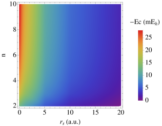
Figure 1: Reduced correlation energies (in ${\rm m}E_{\rm h}$) for $n$-ringium with various $r_{s}$.

Table 6: Reduced correlation energies (in ${\rm m}E_{\rm h}$) for $n$-ringium with various $r_{s}$. Statistical errors in the last digit of the DMC energies are shown in parentheses.

$n\backslash r_{s}$	0	0.1	0.2	0.5	1	5	10	20
2	13.212	12.985	12.766	12.152	11.250	7.111	4.938	3.122
3	18.484	18.107	17.747	16.755	15.346	9.369	6.427	4.029
4	21.174	20.698	20.24(2)	19.00(1)	17.320(1)	10.390(0)	7.085(0)	4.425(0)
5	22.756	22.213	21.66(2)	20.33(1)	18.439(1)	10.946(0)	7.439(0)	4.636(0)
6	23.775	23.184	22.63(2)	21.14(1)	19.137(1)	11.285(0)	7.653(0)	4.762(0)
7	24.476	23.850	23.24(2)	21.70(1)	19.607(1)	11.509(0)	7.795(0)	4.844(0)
8	24.981	24.328	23.69(3)	22.11(1)	19.940(1)	11.664(0)	7.890(0)	4.901(0)
9	25.360	24.686	24.04(2)	22.39(1)	20.186(1)	11.777(0)	7.960(0)	4.941(0)
10	25.651	24.960	24.25(4)	22.62(1)	20.373(1)	11.857(0)	8.013(0)	4.973(0)
⋮	⋮	⋮	⋮	⋮	⋮	⋮	⋮	⋮
$\infty$	27.416	26.597	25.91(1)	23.962(1)	21.444(0)	12.318(0)	8.292(0)	5.133(0)

V Conclusions

We have studied $n$-ringium using explicitly correlated and quantum Monte Carlo methods. Using Hylleraas wave functions, we have obtained the near-exact ground-state energy of the $n=2$ and $n=3$ systems for various values of the Seitz radius $r_{s}$. For $n\geq 4$, we have performed exact-node DMC calculations to find the exact ground-state energies, with statistical errors in the ${\mu}E_{\rm h}$ range.

We have shown that the reduced correlation energy of $n$-ringium is

$$\epsilon_{\rm c}(r_{s},n)=\epsilon_{2}(n)+\epsilon_{3}(n)r_{s}+\ldots$$ (50)

for high densities, and

$$\epsilon_{\rm c}(r_{s},n)=\frac{\eta_{0}(n)-\epsilon_{1}(n)}{r_{s}}+\frac{\eta_{1}(n)}{r_{s}^{3/2}}+\ldots$$ (51)

for low densities. Expressions for the coefficients are given in Eqs. (28), (II.1.5), (34), (24) and (35).

In the thermodynamic limit, we have found that

$$\epsilon_{\rm c}(r_{s}) =-\frac{\pi^{2}}{360}+0.008446\,r_{s}+\ldots,$$ (52)

$$\epsilon_{\rm c}(r_{s}) =-\frac{\ln(\sqrt{2\pi})-3/4}{r_{s}}+\frac{0.359933}{r_{s}^{3/2}}+\ldots,$$ (53)

and shown that the ringium and jellium models are equivalent in the thermodynamic limit.

This provides a detailed picture of the energy of this new model over a wide range of $n$ and $r_{s}$ values and we believe that the correlation energies in Table 6 are the most accurate yet reported for $n$-ringium. These systems are distinct uniform electron gases Gill and Loos (2012) and can be used to design a new correlation functional for 1D systems. We will report such a functional in a forthcoming paper. Loos and Gill

Appendix

For the ground state, the Hamiltonian (4) can be recast as

$$H=\sum_{i<j}^{n}\left[\left(\frac{r_{ij}^{2}}{4R^{2}}-1\right)\frac{\partial^{2}}{\partial r_{ij}^{2}}+\frac{r_{ij}}{4R^{2}}\frac{\partial}{\partial r_{ij}}+\frac{1}{r_{ij}}\right]+\sum_{\begin{subarray}{c}i\neq j\\ i\neq k\end{subarray}}^{n}\sum_{j<k}^{n}\frac{r_{ik}^{2}+r_{jk}^{2}-r_{ij}^{2}}{2\,r_{ik}r_{jk}}\frac{r_{ij}^{2}+r_{jk}^{2}-r_{ik}^{2}}{2\,r_{ij}r_{jk}}\frac{\partial^{2}}{\partial r_{ij}\partial r_{ik}}.$$ (54)

The first term in (54) contains the two-body parts of the Hamiltonian while the second includes coupling between electron pairs.

The $n$-electron overlap integrals needed in calculations on $n$-ringium can be systematically constructed using the unit-ring Fourier resolution

$$r_{ij}^{m}=\sum_{k=-\infty}^{\infty}B_{m,k}\ e^{ik\theta_{i}}e^{-ik\theta_{j}},$$ (55)

where

$$B_{m,k}=\frac{(-1)^{k}m!}{(m/2+k)!(m/2-k)!}$$ (56)

is a signed binomial coefficient. Eq. (55) is valid for $m\geq 0$ and terminates if $m$ is an even integer.

Resolving each integrand factor, swapping the order of summation and integration, performing the integrations and resumming, often leads to beautiful expressions. For example, the cyclic $n$-electron integral yields

$$\langle r_{12}^{a}r_{23}^{b}r_{34}^{c}\ldots r_{n,1}^{z}\rangle=\sum_{k=-\infty}^{\infty}B_{a,k}B_{b,k}B_{c,k}\ldots B_{z,k},$$ (57)

which can be written as a ${}_{n+1}F_{n}$ hypergeometric function of unit argument. Olver et al. (2010)

In some cases, the sums can be found in closed form, for example,

$$\langle r_{ij}^{a}\rangle=B_{a,0},$$ (58)

$$\langle r_{ij}^{a}r_{kl}^{b}\rangle=B_{a,0}B_{b,0},$$ (59)

$$\langle r_{12}^{a}r_{23}^{b}r_{31}^{c}\rangle=\frac{a!\,b!\,c!}{\left(\frac{a+b}{2}\right)!\left(\frac{a+c}{2}\right)!\left(\frac{b+c}{2}\right)!}\frac{\left(\frac{a+b+c}{2}\right)!}{\left(\frac{a}{2}\right)!\left(\frac{b}{2}\right)!\left(\frac{c}{2}\right)!},$$ (60)

but this is not possible in general. de Bruijn (1981) (Eq. (60) uses the result of Problem 62 of Knuth’s book. Knuth (1969)) However, sums such as (57) converge rapidly and are numerically satisfactory.

References

- Gill and Loos (2012) P. M. W. Gill and P. F. Loos, Theor. Chem. Acc. 131, 1069 (2012).
- Giuliani and Vignale (2005) G. F. Giuliani and G. Vignale, Quantum theory of the electron liquid (Cambridge University Press, Cambridge, 2005).
- Loos and Gill (2011a) P. F. Loos and P. M. W. Gill, Phys. Rev. B 83, 233102 (2011a).
- Loos and Gill (2011b) P. F. Loos and P. M. W. Gill, Phys. Rev. B 84, 033103 (2011b).
- Parr and Yang (1989) R. G. Parr and W. Yang, Density Functional Theory for Atoms and Molecules (Oxford University Press, 1989).
- Loos and Gill (2011c) P. F. Loos and P. M. W. Gill, J. Chem. Phys. 135, 214111 (2011c).
- Loos and Gill (2009a) P. F. Loos and P. M. W. Gill, Phys. Rev. A 79, 062517 (2009a).
- Loos and Gill (2009b) P. F. Loos and P. M. W. Gill, Phys. Rev. Lett. 103, 123008 (2009b).
- Loos and Gill (2010a) P. F. Loos and P. M. W. Gill, Phys. Rev. A 81, 052510 (2010a).
- Loos (2010) P. F. Loos, Phys. Rev. A 81, 032510 (2010).
- Loos and Gill (2010b) P. F. Loos and P. M. W. Gill, Mol. Phys. 108, 2527 (2010b).
- Loos (2012) P. F. Loos, Phys. Lett. A 376, 1997 (2012).
- Pederiva and Lipparini (2002) F. Pederiva and E. Lipparini, Phys. Rev. B 66, 165314 (2002).
- Casula, Sorella, and Senatore (2006) M. Casula, S. Sorella, and G. Senatore, Phys. Rev. B 74, 245427 (2006).
- Lee and Drummond (2011) R. M. Lee and N. D. Drummond, Phys. Rev. B 83, 245114 (2011).
- Schulz (1993) H. J. Schulz, Phys. Rev. Lett. 71, 1864 (1993).
- Fogler (2005) M. M. Fogler, Phys. Rev. Lett. 94, 056405 (2005).
- Astrakharchik and Girardeau (2011) G. E. Astrakharchik and M. D. Girardeau, Phys. Rev. B 83, 153303 (2011).
- Loos and Gill (2012) P. F. Loos and P. M. W. Gill, Phys. Rev. Lett. 108, 083002 (2012).
- Kato (1957) T. Kato, Commun. Pure Appl. Math. 10, 151 (1957).
- Girardeau (1960) M. D. Girardeau, J. Math. Phys. 1, 516 (1960).
- Warburton et al. (2000) R. J. Warburton, C. Schäflein, D. Haft, F. Bickel, A. Lorke, K. Karrai, J. M. Garcia, W. Schoenfeld, and P. M. Petroff, Nature 405, 926 (2000).
- Fuhrer et al. (2001) A. Fuhrer, S. Luscher, T. Ihn, T. Heinzel, K. Ensslin, W. Wegscheider, and M. Bichler, Nature 413, 822 (2001).
- Lorke et al. (2000) A. Lorke, R. Johannes Luyken, A. O. Govorov, J. P. Kotthaus, J. M. Garcia, and P. M. Petroff, Phys. Rev. Lett. 84, 2223 (2000).
- Keyser et al. (2003) U. F. Keyser, C. Fuhner, S. Borck, R. J. Haug, M. Bichler, G. Abstreiter, and W. Wegscheider, Phys. Rev. Lett. 90, 196601 (2003).
- Mailly, Chapelier, and Benoit (1993) D. Mailly, C. Chapelier, and A. Benoit, Phys. Rev. Lett. 70, 2020 (1993).
- Bayer et al. (2003) M. Bayer, M. Korkusinski, P. Hawrylak, T. Gutbrod, M. Michel, and A. Forchel, Phys. Rev. Lett. 90, 186801 (2003).
- Fuhrer et al. (2004) A. Fuhrer, T. Ihn, K. Ensslin, W. Wegscheider, and M. Bichler, Phys. Rev. Lett. 93, 176803 (2004).
- Sigrist et al. (2004) M. Sigrist, A. Fuhrer, T. Ihn, K. Ensslin, S. E. Ulloa, W. Wegscheider, and M. Bichler, Phys. Rev. Lett. 93, 066802 (2004).
- Viefers et al. (2004) S. Viefers, P. Koskinen, P. Singha Deo, and M. Manninen, Physica E 21, 1 (2004).
- Fogler and Pivovarov (2005) M. M. Fogler and E. Pivovarov, Phys. Rev. B 72, 195344 (2005).
- Fogler and Pivovarov (2006) M. M. Fogler and E. Pivovarov, J. Phys.: Condens. Matter 18, L7 (2006).
- Niemela et al. (1996) K. Niemela, P. Pietilainen, P. Hyvonen, and T. Chakraborty, Europhys. Lett. 36, 533 (1996).
- Gylfadottir et al. (2006) S. S. Gylfadottir, A. Harju, T. Jouttenus, and C. Webb, New J. Phys. 8, 211 (2006).
- Emperador, Pederiva, and Lipparini (2003) A. Emperador, F. Pederiva, and E. Lipparini, Phys. Rev. B 68, 115312 (2003).
- Emperador et al. (2001) A. Emperador, M. Pi, M. Barranco, and E. Lipparini, Phys. Rev. B 64, 155304 (2001).
- Räsänen et al. (2009) E. Räsänen, S. Pittalis, C. R. Proetto, and E. K. U. Gross, Phys. Rev. B 79, 121305 (2009).
- Aichinger et al. (2006) M. Aichinger, S. A. Chin, E. Krotscheck, and E. Räsänen, Phys. Rev. B 73, 195310 (2006).
- Manninen and Reimann (2009) M. Manninen and S. M. Reimann, J. Phys. A: Math. Theor. 42, 214019 (2009).
- Aharonov and Bohm (1959) Y. Aharonov and D. Bohm, Phys. Rev. 115, 485 (1959).
- Aronov and Lyanda-Geller (1993) A. G. Aronov and Y. B. Lyanda-Geller, Phys. Rev. Lett. 70, 343 (1993).
- Morpurgo et al. (1998) A. F. Morpurgo, J. P. Heida, T. M. Klapwijk, B. J. van Wees, and G. Borghs, Phys. Rev. Lett. 80, 1050 (1998).
- Gell-Mann and Brueckner (1957) M. Gell-Mann and K. A. Brueckner, Phys. Rev. 106, 364 (1957).
- Wigner (1934) E. Wigner, Phys. Rev. 46, 1002 (1934).
- McMillan (1965) W. L. McMillan, Phys. Rev. 138, A442 (1965).
- Ceperley, Chester, and Kalos (1977) D. Ceperley, G. V. Chester, and M. H. Kalos, Phys. Rev. B 16, 3081 (1977).
- Umrigar (1999) C. J. Umrigar, “Quantum monte carlo methods in physics and chemistry,” (Kluwer Academic Press, Dordrecht, 1999) pp. 129–160.
- Kalos, Levesque, and Verlet (1974) M. H. Kalos, D. Levesque, and L. Verlet, Phys. Rev. A 9, 2178 (1974).
- Ceperley and Kalos (1979) D. M. Ceperley and M. H. Kalos, “Monte carlo methods in statistical physics,” (Springer Verlag, Berlin, 1979).
- Reynolds et al. (1982) P. J. Reynolds, D. M. Ceperley, B. J. Alder, and W. A. Lester, Jr., J. Chem. Phys. 77, 5593 (1982).
- Nemec (2010) N. Nemec, Phys. Rev. B 81, 035119 (2010).
- Mitas (2006) L. Mitas, Phys. Rev. Lett. 96, 240402 (2006).
- Olver et al. (2010) F. W. J. Olver, D. W. Lozier, R. F. Boisvert, and C. W. Clark, eds., NIST handbook of mathematical functions (Cambridge University Press, New York, 2010).
- Loos (2013) P. F. Loos, J. Chem. Phys. 138, 064108 (2013).
- Rajagopal and Kimball (1977) A. K. Rajagopal and J. C. Kimball, Phys. Rev. B 15, 2819 (1977).
- Thomson (1904) J. J. Thomson, Phil. Mag. Ser. 6 7, 237 (1904).
- Loos and Gill (2010c) P. F. Loos and P. M. W. Gill, Chem. Phys. Lett. 500, 1 (2010c).
- Loos and Gill (2010d) P. F. Loos and P. M. W. Gill, Phys. Rev. Lett. 105, 113001 (2010d).
- Hylleraas (1929) E. A. Hylleraas, Z. Phys. 54, 347 (1929).
- Hylleraas (1930) E. A. Hylleraas, Z. Phys. 65, 209 (1930).
- Hylleraas (1964) E. A. Hylleraas, Adv. Quantum Chem. 1, 1 (1964).
- Jastrow (1955) R. Jastrow, Phys. Rev. 98, 1479 (1955).
- Lee et al. (2011) R. M. Lee, G. J. Conduit, N. Nemec, P. Lopez-Rios, and N. D. Drummond, Phys. Rev. E 83, 066706 (2011).
- Kolorenc and Mitas (2011) J. Kolorenc and L. Mitas, Rep. Prog. Phys. 74, 026502 (2011).
- Umrigar, Nightingale, and Runge (1993) C. J. Umrigar, M. P. Nightingale, and K. J. Runge, J. Chem. Phys. 99, 2865 (1993).
- Huang, Umrigar, and Nightingale (1997) C.-J. Huang, C. J. Umrigar, and M. P. Nightingale, J. Chem. Phys. 107, 3007 (1997).
- Umrigar and Filippi (2005) C. J. Umrigar and C. Filippi, Phys. Rev. Lett. 94, 150201 (2005).
- Toulouse and Umrigar (2007) J. Toulouse and C. J. Umrigar, J. Chem. Phys. 126, 084102 (2007).
- Loh et al. (1990) E. Y. Loh, J. E. Gubernatis, R. T. Scalettar, S. R. White, D. J. Scalapino, and R. L. Sugar, Phys. Rev. B 41, 9301 (1990).
- Troyer and Wiese (2005) M. Troyer and U.-J. Wiese, Phys. Rev. Lett. 94, 170201 (2005).
- Umrigar et al. (2007) C. J. Umrigar, J. Toulouse, C. Filippi, S. Sorella, and R. G. Hennig, Phys. Rev. Lett. 98, 110201 (2007).
- Ceperley (1991) D. M. Ceperley, J. Stat. Phys. 63, 1237 (1991).
- Needs et al. (2010) R. J. Needs, M. D. Towler, N. D. Drummond, and P. Lopez-Rios, J. Phys.: Condensed Matter 22, 023201 (2010).
- (74) P. F. Loos and P. M. W. Gill, J. Chem. Phys. , in preparation.
- de Bruijn (1981) N. G. de Bruijn, Asymptotic Methods in Analysis (Dover, New York, 1981).
- Knuth (1969) D. Knuth, The Art of Computer Programming, Vol. 1. Fundamental algorithms (Addison-Wesley, Reading, MA, 1969).