More Reliable Measurements of the Slip Length with the Atomic Force Microscope

Abstract

Further improvements are made to the non-linear data analysis algorithm for the atomic force microscope [P. Attard, arXiv:1212.3019v2 (2012)]. The algorithm is required when there is curvature in the compliance region due to photo-diode non-linearity. Results are obtained for the hydrodynamic drainage force, for three surfaces: hydrophilic silica (symmetric, Si-Si), hydrophobic dichlorodimethylsilane (symmetric, DCDMS-DCDMS), and hydrophobic octadecyltrichlorosilane (asymmetric, Si-OTS). The drainage force was measured in the viscous liquid di-n-octylphthalate. The slip-lengths are found to be $3\,$nm for Si, $2\,$nm for DCDMS, and $2\,$nm for OTS, with an uncertainty on the order of a nanometer. These slip lengths are a factor of 4–15 times smaller than those obtained from previous analysis of the same raw data [L. Zhu et al., Langmuir, 27, 6712 (2011). Ibid, 28, 7768 (2012)].

I Introduction

Measurements of the slip length are significant for three reasons. First, the hydrodynamic equations for any flow can’t be solved without specifying the boundary conditions, and so whether a fluid sticks or slips during shear flow at a solid surface is fundamental to the application of hydrodynamics to the real world. In turn, the extent that a fluid slips, if any, effects quantitatively a range of physical phenomena (e.g. flow rates in pores, drainage forces between particles, lubrication of surfaces, pressure heads in microfluidic devices), and so measuring, understanding, and controlling slip could lead to new technologies, devices, and industrial processes.

Second, whereas equilibrium statistical mechanics is well-established for elucidating static molecular structure (in bulk and at surfaces), the same cannot be said for the non-equilibrium case, either in general or for fluid flow. Hence nanoscopic measurements of the slip length yield fundamental information about the structure of the fluid and its interaction with the solid surface during shear flow. Such data is valuable in its own right, providing molecular-level insight into inhomogeneous flow and perhaps enabling one to identify the specifically non-equilibrium aspects of the way in which structure, flow, and interaction are entwined at the molecular level. In turn the measurements provide specific motivation to develop non-equilibrium computer simulations, and benchmarks against which those algorithms could be tested.

Third, slip can be regarded as a correction to stick boundary conditions, and as such it is a second order effect that is a real challenge to measure experimentally with any reliability or accuracy. Obviously any small error in the measurement overall translates into a large error in the slip length. The literature abounds with examples where the reported slip lengths vary by an order of magnitude for ostensibly the same system. Neto05 ; Bocquet10 (The present paper will present slip lengths that are a factor of 15 smaller than those previously reported for the same data.) Hence credible measurements of the slip length can only be obtained by improving the reliability and accuracy of the measurement technique itself, and this would have broad benefits beyond the immediate application to slip.

On this last point, the present paper uses the atomic force microscope to measure the slip length via the analysis of the hydrodynamic drainage force. The present results represent the third generation of improvements to atomic force microscopy that have been motivated by the desire for reliable measurements of the slip length. Most of the new algorithms and procedures are general in nature and can be directly applied to other forces measured with the atomic force microscope. In the present case, where the sought for slip length is a second order effect, the new procedures have proved essential for reliable results. In other cases, where one might be measuring a first order effect, the improvements are still worthwhile because they reduce the quantitative error of the measurements by about an order of magnitude while still remaining simple enough for the data analysis to be carried out by a spreadsheet.

Figure 1: The raw photo-diode voltage versus the piezo-drive displacement. The solid curve is measured extension data, the dashed line gives the tangent at first contact, and the dotted line gives the average slope in contact. The inset shows the analysed force versus separation, with the solid curve resulting from the non-linear analysis and the dashed and dotted curves resulting from the conventional linear analysis using the first contact slope and the average slope, respectively. The source of the measured data is Ref. Zhu12, , which may be consulted for the experimental details.

In Appendix A, the various improvements in force measurement and data analysis with the atomic force microscope are summarized. The focus is on those developments stimulated by the challenge of accurate and reliable measurements of the slip length, although of course many of these improvements are more generally applicable. As discussed in the appendix, the most recent series of improvements concern the non-linear analysis of the measured force data.Attard12 The need for such an algorithm arises when the compliance region has curvature, as is shown in Fig. 1. The non-linearity is due to the response of the photo-diode, most likely arising from non-uniformity in intensity and width of the light beam moving across the split photo-diode. In Ref. Attard12, , an algorithm was given based on a polynomial of best fit to the contact region, from which the angular and vertical deflection of the cantilever in the non-contact region can be obtained. The algorithm was applied to measured raw data for the drainage force in the Si-DOPC-Si system.

This paper presents further improvements to the non-linear data analysis algorithm that are applicable to general atomic force microscopy. The modified analysis is applied to two new systems, DCDMS-DOPC-DCDMS and Si-DOPC-OTS, as well as re-analysing the Si-DOPC-Si system.

One improvement concerns replacing an extrapolation of the polynomial fit by an inherently more reliable interpolation. This can be explained as follows. The voltage measured on extension can be split into two ranges, in contact $V\geq V_{\mathrm{c,ext}}$, and prior to contact $V\leq V_{\mathrm{c,ext}}$ (because the drainage force is repulsive), where $V_{\mathrm{c,ext}}$ is the voltage at initial contact. This means that in order to obtain the pre-contact drainage force on extension from the measured voltage, one has to use an extrapolation of the non-linear fit made in contact. This extrapolation can lead to small but unacceptable errors. In contrast, on retraction, in contact the voltage is $V\geq V_{\mathrm{c,ret}}$, and after contact $V\gtrsim V_{\mathrm{c,ret}}$ (because the drainage force is attractive), the voltage at final contact, $V_{\mathrm{c,ret}}$, is strictly less than the voltage measured on the whole range of extension. This means that one can use the non-linear fit to the retraction data in contact to obtain both the extension and the retraction out of contact force by interpolation rather than extrapolation. This gives a small but significant improvement in the drainage results.

A second improvement is that a least squares fit algorithm has been developed to obtain the cantilever spring constant and effective drag length from the measured data at large separations. By automating this procedure, a source of possible human bias is eliminated and the time required to analyze each force curve is significantly reduced.

A third improvement was also explored, which in some systems can be important, but which makes negligible difference for the atomic force microscope data analyzed here. This is variable cantilever drag, which arises from the fact that the hydrodynamic drag on the cantilever decreases as the cantilever bends in response to the drainage force. This effect was not taken into account in the theoretical forces that were fitted to the non-linearly analyzed data.Attard12 In earlier linear analysis, variable drag was found to be significant for weak cantilevers ($k_{\mathrm{eff}}\lesssim.1\,$N/m), but negligible for stiff ones($k_{\mathrm{eff}}\gtrsim 1\,$N/m). Zhu11a ; Zhu11b ; Zhu12a Since the spring constant obtained with the non-linear analysis was relatively large, $k_{\mathrm{eff}}=1.68\,$N/m,Attard12 it was assumed that it would be acceptable in the first instance to neglect variable drag. In the present work this assumption is checked by performing variable drag calculations for the experimental conditions, and it is found that it does indeed have negligible effect. However in the process of performing the check, a more robust numerical algorithm was developed that gives more reliable results and that allows the retract data to be calculated as well. This algorithm has some intrinsic interest and is included in Appendix B, which sets out in detail the non-linear data analysis algorithm.

For an independent experimental test of the present protocols, the procedure used in Ref. Zhu12, is used here as well. In that case three sets of measurements were performed for the drainage force in the liquid DOPC (di-n-octylphthalate): Si-Si, DCDMS-DCDMS, and Si-OTS, where Si is a silicon wafer with a native silicon oxide layer, DCDMS is a dichlorodimethylsilane self-assembled monolayer prepared on the same type of silicon wafer from the vapor phase, and OTS is an octadecyltrichlorosilane self-assembled monolayer also prepared on a silicon wafer. In water, Si is hydrophilic with a contact angle close to zero, whereas DCDMS is hydrophobic with an advancing contact angle of 109^∘,Zhu12 and OTS is also hydrophobic with contact angle of 112^∘.Zhu11b In DOPC the contact angle is 21^∘ for Si,Zhu12 48^∘ for DCDMS,Zhu12 and 45^∘ for OTS.Zhu11b Given the similarity of the two hydrophobic monolayers, one would expect them to have similar slip lengths, and the two slip lengths fitted for the symmetric systems ought also fit the asymmetric system. This represents a test of the reliability of the measurement protocol.

II Results

Table 1: Parameters and results for three series of drainage force measurements.^∗

	Si-Si	DCDMS-DCDMS	Si-OTS
No. Meas.	9	11	10
Cantilever†	C	A	F
$L_{0}$ ($\mu$m)	110	90	230
$R$ ($\mu$m)	10.11	9.28	10.14
$k_{0}$ (N/m)	$1.38\pm.06$	$1.78\pm.10$	$1.20\pm.07$
$k_{\mathrm{eff}}$ (N/m)	$1.69\pm.08$	$2.22\pm.12$	$1.34\pm.08$
$L_{\mathrm{drag}}$ ($\mu$m)	$85\pm 8$	$71\pm 5$	$162\pm 5$
$A$ (J m-2)	$1\times 10^{-21}$	$5\times 10^{-20}$	$1\times 10^{-20}$
$b$ (nm)	3	2	3,2

^∗All measurements were performed in di-n-octylphthalate (DOPC), with viscosity $\eta=$ 50–54 mPa s. The average and standard deviation over different drive velocities are given. Here $L_{0}$ is the length of the cantilever, $R$ is the radius of the colloid probe, the $k$ are cantilever spring constants (see text), $L_{\mathrm{drag}}$ is the effective drag length, $A$ is the Hamaker constant, and $b$ is the slip length.

^†NSC12, tipless, rectangular (Mikromasch).

Raw data for three systems were analysed: Si-Si, DCDMS-DCDMS, and Si-OTS. These are summarised in Table 1. The tilt angle of the cantilever was $-11^{\circ}$. The cantilever length quoted in the table is $L_{0}=L_{0}^{*}-2R$, where $L_{0}^{*}$ is the nominal length quoted by the manufacturer. This recipe accounts approximately for the fact that the colloid probe is mounted slightly back from the leading edge of the cantilever.

There is a one-to-one relationship between the intrinsic cantilever spring constant $k_{0}$ and the effective force measuring spring constant $k_{\mathrm{eff}}$, which is given in Eq. (C.3) below. Usually both are quoted below even though this is redundant. In brief, the effective spring constant gives the surface force from the vertical deflection of the contact point, $F_{z}=k_{\mathrm{eff}}z_{\mathrm{c}}$, whereas the intrinsic cantilever spring constant gives the hypothetical force acting normal to the axis of the cantilever that would cause a deflection of the cantilever also normal to its axis, $F_{\perp}=k_{0}\zeta$. Most calibration techniques yield $k_{0}$ and this is what is usually quoted and used in papers even though it is $k_{\mathrm{eff}}$ that is required for the quantitative analysis of atomic force microscopy. In the present paper the spring constant was determined by a least squares fit of the drainage and drag force to the measured data at large separations. The error is about one third of the standard deviation shown in Table 1.

In the figures below the vertical deflection of the contact point $z_{\mathrm{c}}$ is generally given. In previous papers this was called the vertical deflection of the tip and was denoted $z_{\mathrm{t}}$.Zhu11a ; Attard12 It is more precise to call it the vertical deflection of the contact point, and to instead write $\zeta_{L}C_{0}$ for the vertical component of the deflection of the end of the cantilever (see §C.3). In contact, $\Delta z_{\mathrm{c}}=-\Delta z_{\mathrm{p}}$, where $z_{\mathrm{p}}$ is the piezo-drive position. As just mentioned, the surface force is related to this by $F_{z}=k_{\mathrm{eff}}z_{\mathrm{c}}$.

In the deflection-separation curves given below, the constant cantilever drag force has been subtracted. The theoretical calculations also have constant drag subtracted. Calculations have been made with constant and with variable cantilever drag. For the three systems treated below, the effect of variable drag is negligible. The variable drag algorithm used in places below improves upon the originalZhu11a in that it is more robust (in fact, it is more reliable than the spread sheet algorithm for constant drag), it includes tilt and torque, and results are obtained for adhesion and retraction.

II.1 Si-Si

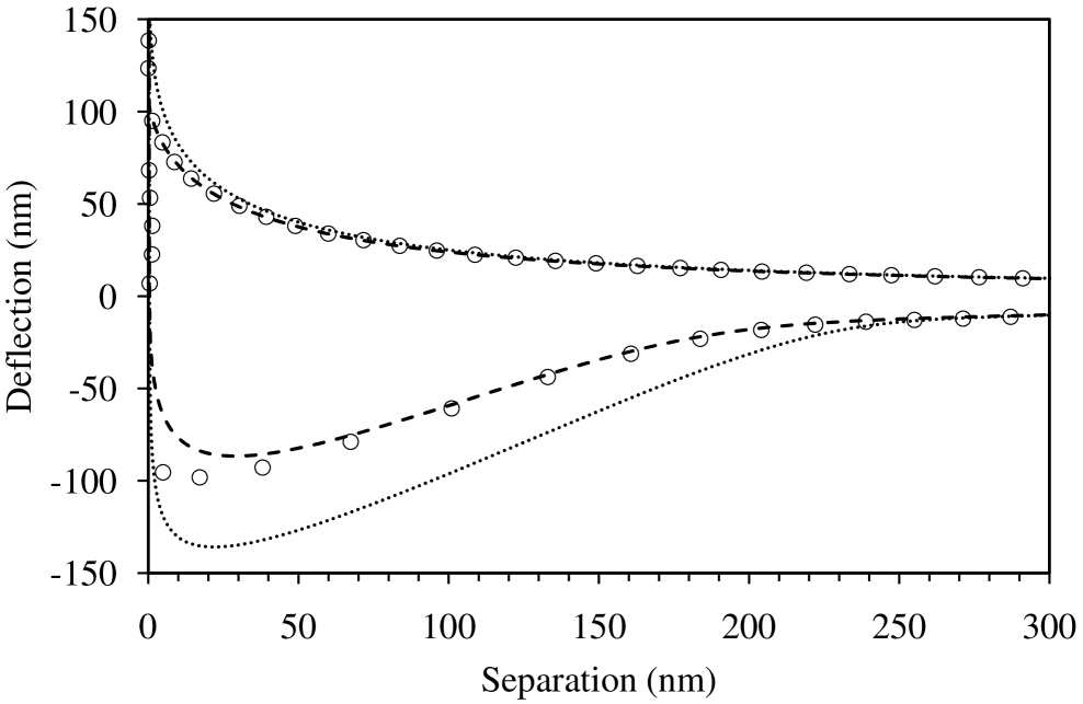
Figure 2: Vertical cantilever deflection $z_{\mathrm{c}}$ versus separation $h$ at a drive rate of $\dot{z}_{\mathrm{p}}=50\,\mu$m s^-1 for Si-Si (see Table 1). The effective cantilever spring constant is $k_{\mathrm{eff}}=1.69\,$N/m. The circles are the analysed experimental measurement (every tenth point plotted), the dotted curve is the calculation with stick boundary conditions, $b=0$ nm, and the dashed curve is the slip calculation, $b=3$ nm. The source of the raw measured data is Ref. Zhu12, .

Figure 2 shows atomic force microscope measurements of the drainage force for Si-Si. The vertical cantilever deflection is shown, from which the force may be obtained as $F_{z}=k_{\mathrm{eff}}z_{\mathrm{c}}$. The raw data was analysed using the non-linear procedures described in Appendix B. It can be seen that the drainage force is repulsive on extension (approach) and attractive on retraction (retreat). At large separations there is almost complete overlap between the measured data and the two calculated curves. At small separations, it can be seen that the stick theory significantly overestimates the magnitude of the measured drainage force on both extension and retraction. The slip theory with $b=3$ nm shows an almost perfect fit on extension all the way into contact. The agreement is less good on retraction immediately pulling out of contact, but by about 40 nm the measured and calculated deflection converge.

The same raw data was non-linearly analysed in Ref. Attard12, . The difference in the two is that the present analysis uses the non-linear fit for the voltage in contact on retraction to obtain the cantilever deflection angle out of contact on extension. Also, here the cantilever spring constant was obtained by a least squares fit of stick theory to the large separation data, $h\in[0.9,3.7]\,\mu$m. This was done at each drive velocity and the result averaged over all velocities. In Ref. Attard12, the fit was performed by eye. The value of the spring constant obtained previously was $k_{\mathrm{eff}}=1.68\,$N/m,Attard12 whereas the present least squares fit gave $k_{\mathrm{eff}}=1.69\pm.08\,$N/m, which suggests that the author has a very good eye. The slip length obtained here, $b=3$ nm, is the same as that obtained previously.Attard12 In the original linear analysis of the atomic force microscope data, the spring constant fitted was $k_{\mathrm{eff}}=1.5\,$N/m, and the slip length fitted at low shear rates was $b_{0}=10$ nm.Zhu12

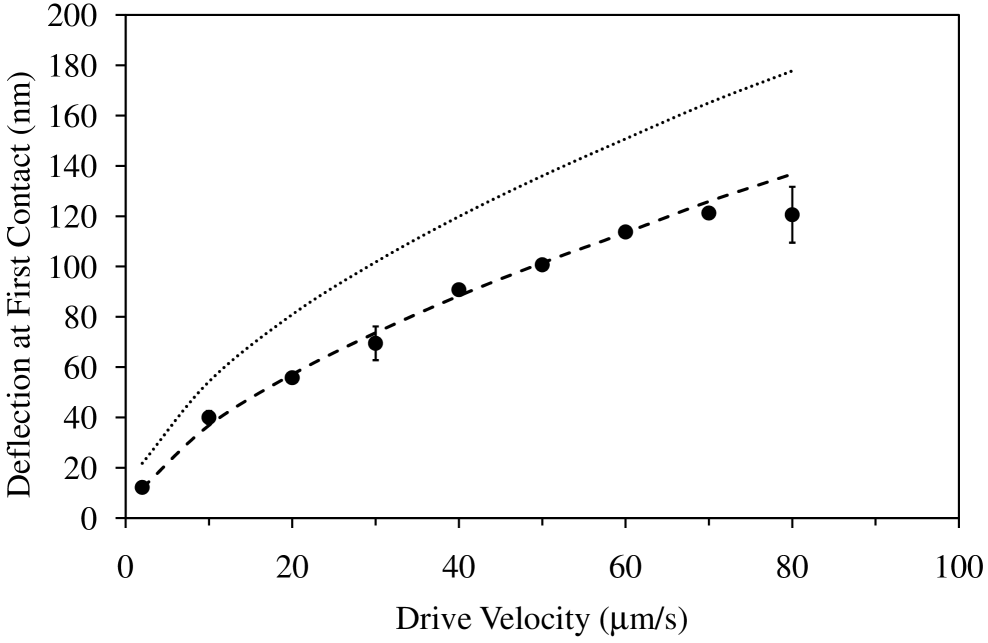
Figure 3: Deflection $z_{\mathrm{c}}$ at first contact versus drive velocity for Si-Si. The symbols are the analysed measured data (raw data from Ref. Zhu12, ), the dotted curve is the stick calculation $b=0$ nm, and the dashed curve is the slip calculation with $b=3$ nm, with other parameters as in Table 1. The bars are a crude estimate of the error arising from the uncertainty in identifying first contact.

The slip theory fits the measured data on extension almost perfectly in Fig. 2, and this level of agreement is reasonably typical of all the forces analysed for Si-Si. This can be seen in Fig. 3, where the cantilever deflection at first contact on extension is shown. In the case of the experiments, there can be an uncertainty (on the order of several nanometers in the drive distance) in deciding exactly where first contact occurs, and it is crudely estimated that this gives an error on the order of 2–10 nm in the deflection. Alternatively, the lack of smoothness in the measured data points in Fig. 3 also gives a guide to the error in the deflection at first contact. Within this error, it can be seen that a slip length of $b=3$ nm gives a deflection at first contact in quantitative agreement with the measured one over the whole range of drive velocities. The stick theory results shown in the figure correspond to $b=0$ nm and overestimate the deflection by about 35% at $\dot{z}=-50\,\mu$m/s. From this one can conclude that any variation in the slip length by more than a fraction of a nanometer will lead to a significantly worse fit than has been obtained for $b=3$ nm.

The van der Waals force has very little effect on the force on extension. For example, at a drive velocity of $\dot{z}=-50\,\mu$m/s, the calculated deflection at first contact for $b=3\,$nm and a Hamaker constant of $A=1.3\times 10^{-21}\,$J m^-2 is 101.4 nm. Changing the Hamaker constant to $A=5\times 10^{-21}\,$J m^-2, the deflection becomes 100.9 nm.

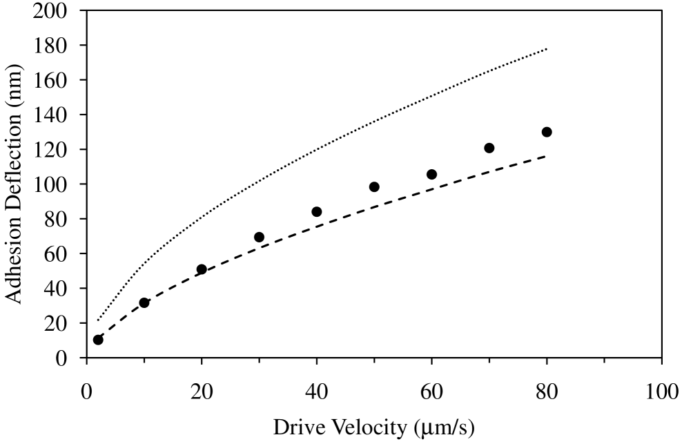
Figure 4: Adhesion deflection $z_{\mathrm{c}}$ versus drive velocity for Si-Si. The symbols, curves and parameters are as in the preceding figure. The adhesive tension is $F_{z}=k_{\mathrm{eff}}z_{\mathrm{c}}$. The calculations use a Hamaker constant of $A=1.3\times 10^{-21}\,$J m^-2 and zero force position of $z_{0}=0.53\,$nm.

Figure 4 shows the adhesion deflection, which is defined as the negative of the minimum deflection that occurs on retraction. This is easier to obtain and shows less variability than the deflection at last contact. In general terms obtaining the adhesion reliably in atomic force microscopy is extremely challenging. This is because the jump out of contact is a catastrophic event and it is exceedingly sensitive to external vibrations, surface roughness, elastic deformation, and to sliding and rolling of the probe, and to peeling of the contact region. The present drainage force appears to be an exception, since there is quite good agreement between theory and measurement in this case. Although the instant of the jump out is variable, the minimum in the force curve, which is the maximum tension, is quite stable and appears to be largely determined by the drainage force.

It can be seen in Fig. 4 that stick theory significantly overestimates the adhesion, whereas slip theory with $b=3\,$nm is relatively accurate. From the high velocity data one might conclude that $b=3\,$nm is an upper bound on the slip length.

Although the actual pull-off deflection at last contact can be sensitive to the van der Waals force, the adhesion deflection as defined here is less so. For example, at a drive velocity of $\dot{z}=-50\,\mu$m/s, the measured adhesion deflection is 98.3 nm. The calculated adhesion deflection for a Hamaker constant of $A=1.3\times 10^{-21}\,$J m^-2 and a slip length of $b=3\,$nm is 86.7 nm, and that for stick, $b=0\,$nm is 136.0 nm. Changing the Hamaker constant to $A=5\times 10^{-21}\,$J m^-2 for the slip length of $b=3\,$nm, the deflection becomes 88.9 nm.

II.2 DCDMS-DCDMS

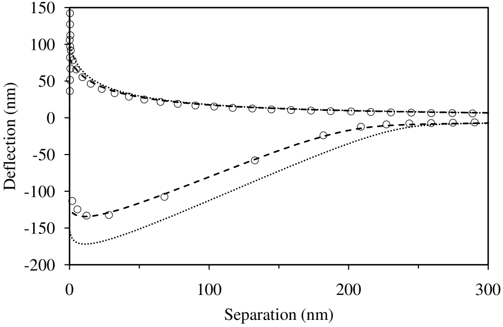
Figure 5: Vertical cantilever deflection $z_{\mathrm{c}}$ versus separation $h$ at a drive rate of $\dot{z}_{\mathrm{p}}=50\,\mu$m s^-1 for DCDMS-DCDMS (see Table 1). The effective cantilever spring constant is $k_{\mathrm{eff}}=2.22\,$N/m. The circles are the analysed experimental measurement (every tenth point plotted), the dotted curve is the stick calculation, $b=0$ nm, and the dashed curve is the slip calculation, $b=2$ nm. The source of the raw measured data is Ref. Zhu12, .

Analysed atomic force microscope results for the vertical deflection of the cantilever as a function of separation for DCDMS-DCDMS are shown in Fig. 5. Again it can be seen that the stick theory overestimates the magnitude of the force at small separations on both extension and retraction. In contrast, the slip theory with $b=2$ nm fits the measured results on extension down to several nanometers from first contact. It is also in surprisingly good agreement for the measured retraction force.

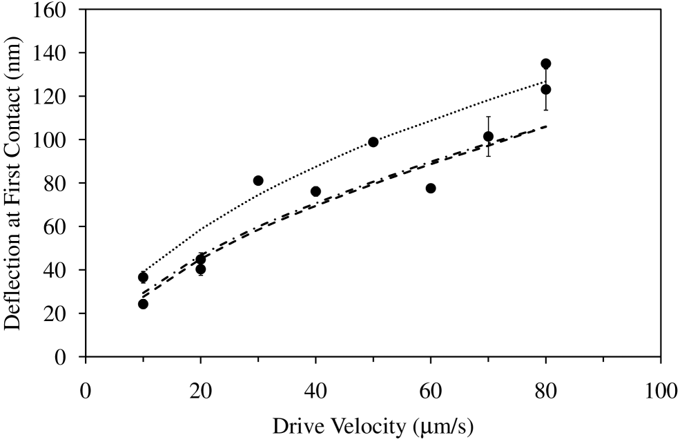
Figure 6: Deflection $z_{\mathrm{c}}$ at first contact versus drive velocity for DCDMS-DCDMS. The symbols are the analysed measured data (raw data from Ref. Zhu12, ), the dotted curve is the stick calculation $b=0$ nm and a Hamaker constant of $A=5\times 10^{-20}\,$J m^-2, the dashed curve is the slip calculation with $b=2$ nm and $A=5\times 10^{-20}\,$J m^-2, and the dash-dotted curve is the slip calculation with $b=2$ nm and $A=1\times 10^{-20}\,$J m^-2. The other parameters are as in Table 1. The bars are a crude estimate of the error arising from the uncertainty in identifying first contact.

The extension deflection at first contact is shown in Fig. 6 as a function of drive velocity, including a number of repeat measurements. There appears to be a larger scatter in the measured data in this case compared to Si-Si analysed in Fig. 3. The crude error estimate appears to be on the low side. Calculated results for $A=5\times 10^{-20}\,$J m^-2, and for $A=1\times 10^{-20}\,$J m^-2 are shown to give an idea of the sensitivity to the Hamaker constant. Most of the measured data lie between $b=0$ nm and $b=2$ nm. It is a little unexpected that the slip length for the hydrophobic low energy surface DCDMS should be less than the slip length for the hydrophilic high energy surface Si.

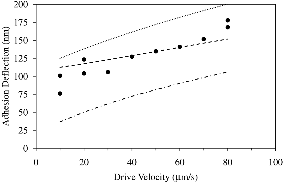
Figure 7: Adhesion deflection $z_{\mathrm{c}}$ versus drive velocity for DCDMS-DCDMS. The symbols, curves, and parameters are as in the preceding figure. The adhesive tension is $F_{z}=k_{\mathrm{eff}}z_{\mathrm{c}}$.

Figure 7 shows the adhesion deflection as a function of drive velocity, again including repeat measurements. Again most of the measured data lie between $b=0$ nm and $b=2$ nm. The Hamaker constant that was used, $A=5\times 10^{-20}\,$J m^-2, is forty times larger that was used for Si-Si. It can be seen that a Hamaker constant of $A=1\times 10^{-20}\,$J m^-2 significantly underestimates the adhesion. (One might argue from the low velocity data that a value of $A=4\times 10^{-20}\,$J m^-2 would give a better fit. One might also argue that a smaller slip length would better fit the high velocity data.) To be concrete, at a drive velocity of $\dot{z}_{\mathrm{p}}=50\,\mu$m s^-1, the measured adhesion deflection is 134.7 nm. For $b=2$ nm and $A=5\times 10^{-20}\,$J m^-2, the calculated adhesion is 133.8 nm, and for $b=2$ nm and $A=1\times 10^{-20}\,$J m^-2, it is 81.3 nm. These calculations were performed with the variable drag algorithm. Using constant drag instead, for $b=2$ nm and $A=5\times 10^{-20}\,$J m^-2, the calculated adhesion is 134.9 nm, which is a minor change. (In this case the deflection at first contact increases by 0.9 nm using constant rather than variable drag.)

II.3 Si-OTS

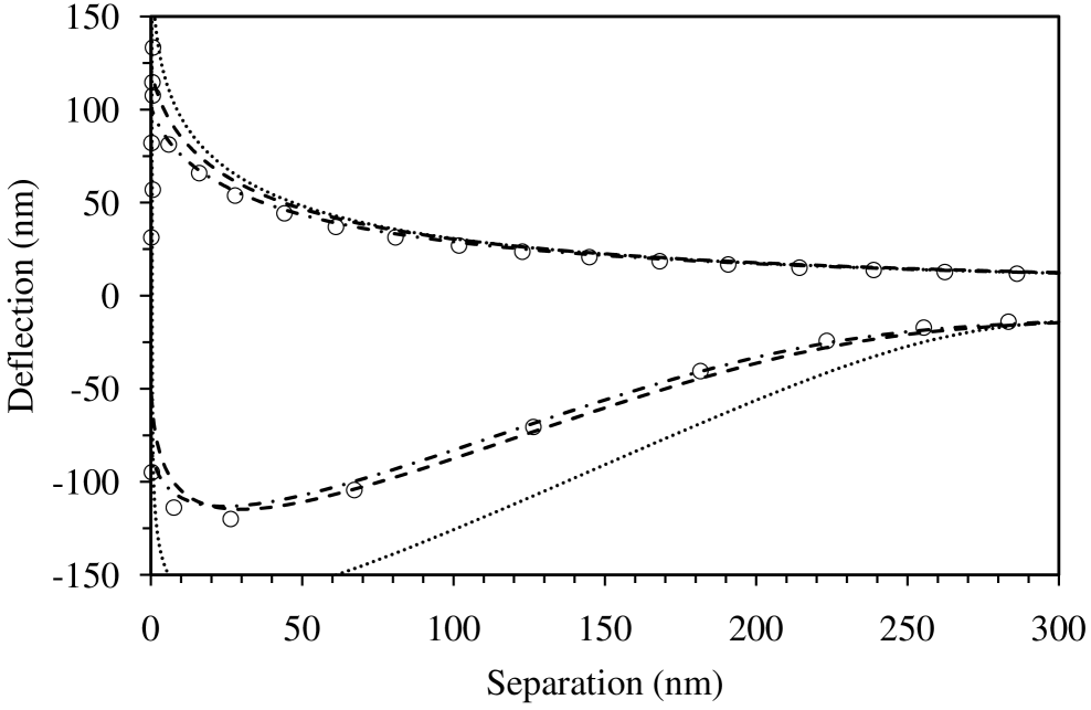
Figure 8: Vertical cantilever deflection $z_{\mathrm{c}}$ versus separation $h$ at a drive rate of $\dot{z}_{\mathrm{p}}=50\,\mu$m s^-1 for Si-OTS (see Table 1). The effective cantilever spring constant is $k_{\mathrm{eff}}=1.34\,$N/m. The circles are the analysed experimental measurement (every tenth point plotted), the dotted curve is the stick calculation, $b_{\mathrm{Si}}=b_{\mathrm{OTS}}=0$ nm, the dashed curve is a slip calculation, $b_{\mathrm{Si}}=3$ nm and $b_{\mathrm{OTS}}=2$ nm, both with a Hamaker constant of $A=1\times 10^{-20}\,$J m^-2, and the dash-dotted curve is a slip calculation with $b_{\mathrm{Si}}=3$ nm, $b_{\mathrm{OTS}}=10$ nm, and $A=2\times 10^{-20}\,$J m^-2. The source of the raw measured data is Ref. Zhu11b, .

Figure 8 shows the measured and calculated drainage force for Si-OTS. Given the similarity in contact angles, the OTS surface is expected to exhibit similar slip characteristics to the DCDMS surface, $b_{\mathrm{DCDMS}}=2$ nm found above. Although $b_{\mathrm{OTS}}=2$ nm is not a bad fit, it can be seen that at small separations on extension, at this velocity the measured data is better fitted with a larger slip length, $b_{\mathrm{OTS}}=10$ nm. Both curves use $b_{\mathrm{Si}}=3$ nm, which was the value found above. For the retract curve, both slip lengths are about equally good. The calculations in the figure were obtained with the variable drag algorithm. There is negligible difference for constant drag.

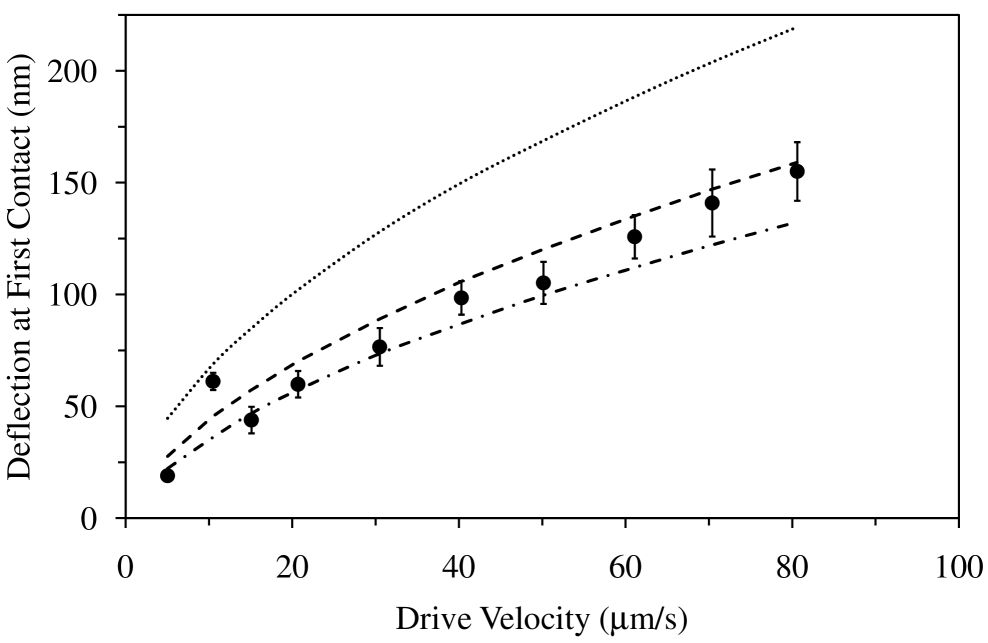
Figure 9: Deflection $z_{\mathrm{c}}$ at first contact versus drive velocity for Si-OTS. The symbols, curves, and parameters are as in the preceding figure. The bars are a crude estimate of the error arising from the uncertainty in identifying first contact.

For the deflection at first contact, Fig. 9, as expected the stick theory overestimates the repulsion due to the drainage force. Within the experimental scatter, there is little to choose between a slip length of $b_{\mathrm{OTS}}=2$ nm and $b_{\mathrm{OTS}}=10$ nm. Perhaps the former is slightly better at high velocities and the latter is slightly better at low velocities. The Hamaker constant has almost no effect on extension (approach).

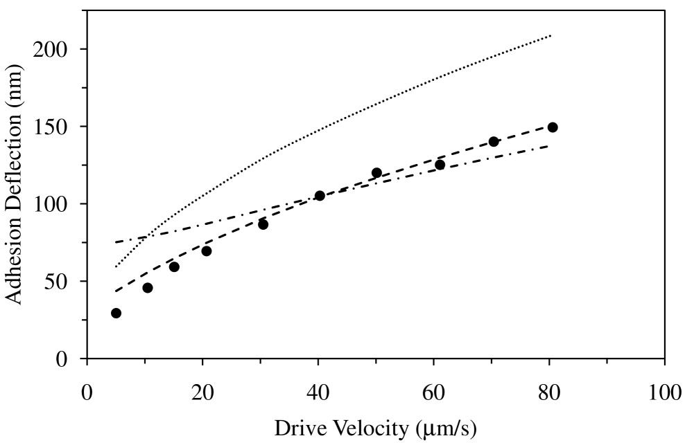
Figure 10: Adhesion deflection $z_{\mathrm{c}}$ versus drive velocity for Si-OTS. The symbols, curves, and parameters are as in the preceding figure. The adhesive tension is $F_{z}=k_{\mathrm{eff}}z_{\mathrm{c}}$.

The adhesion deflection for Si-OTS is shown in Fig. 10. As for the preceding cases, the adhesion increases with increasing velocity, and at each velocity it has about the same magnitude as the deflection at first contact. It can be seen from Fig. 10 that the calculation $b_{\mathrm{Si}}=3$ nm, $b_{\mathrm{OTS}}=10$ nm and $A=2\times 10^{-20}\,$J m^-2 overestimates the adhesion by about 150% at low drive velocities and underestimates it by about 10% at high velocities. Decreasing the Hamaker constant to $A=1\times 10^{-20}\,$J m^-2 improves the fit at low velocities, where it overestimates the adhesion by about 40%, but makes it worse at high velocities, where it underestimates the adhesion by about 15%. Overall, the slip length $b_{\mathrm{OTS}}=2$ nm is in significantly better agreement with the measured adhesion than is the slip length $b_{\mathrm{OTS}}=10$ nm.

For the case of Si-OTS, the deflection at first contact cannot definitively distinguish between $b_{\mathrm{OTS}}=2$ nm and $b_{\mathrm{OTS}}=10$ nm. However, based on the results for the adhesion deflection, one can say that the slip length is much closer to $b_{\mathrm{OTS}}=2$ nm than it is to $b_{\mathrm{OTS}}=10$ nm. The former value is the same as that found for the similar hydrophobic surface, $b_{\mathrm{DCDMS}}=2$ nm.

III Conclusion

The non-linear algorithm for the analysis of atomic force microscopy data has been improved and made more reliable here. Specifically, the conversion of voltage to cantilever deflection is now more reliable on extension out of contact. Also the spring constant is more reliable as it is now determined by a least squares fitting procedure.

Previously measured raw dataZhu12 ; Zhu11b was re-analyzed with the non-linear algorithm. For silica, the slip length was found to be 3 nm, for dichlorodimethylsilane it was 2 nm, and for octadecyltrichlorosilane it was 2 nm. These values are from 3–15 times smaller than those originally obtained with the linear analysis of the same data. Zhu12 ; Zhu11b It is of note that the two low energy surfaces have a smaller slip length than the high energy silica surface.

Hamaker constants for the van der Waals force were also obtained from the measured retraction data. For Si-DOPC-Si the Hamaker constant was found to be $1\times 10^{-21}$ J m^-2, for DCDMS-DOPC-DCDMS it was $5\times 10^{-20}$ J m^-2, and for Si-DOPC-OTS it was $1\times 10^{-20}$ J m^-2. In so far as OTS is similar to DCDMS, the fact that the asymmetric system lies intermediate between the two symmetric systems is physically reasonable.

Appendix A Improvements in Atomic Force Microscopy

One of the crucial issues is the calibration of the cantilever that is used to measure the surface forces: using too small a value for the spring constant causes the slip length to be overestimated and conversely if it is too large. Hence motivated by the need for accurate values, one significant improvement in atomic force measurement methodology was the in situ measurement of the spring constant of the cantilever.Craig01 This was done by measuring the drainage force at large separations, and only required values of the radius of the colloid probe and the viscosity of the liquid, both of which can be readily measured. This method has three advantages: First, as an in situ measurement the effective spring constant that emerges is the one that is required for the actual measurements that are being performed. In particular, it automatically takes into account the position at which the colloid probe is glued to the cantilever (the cantilever spring constant varies as the cube of the distance from the base), and also the tilt of the cantilever, which is typically about $-11^{\circ}$ (the force measuring spring constant varies as the square of the cosine of the tilt angle). Second, the statistical error is much reduced, being on the order of 1% for the hydrodynamic method compared to 10–20% for the thermal method, for example. Third, as has been pointed out,Attard06a the most common conventional method of spring constant calibration, the thermal method, suffers from a mathematical error in an early publication,Higgins06 which has been faithfully reproduced in the built-in software of at least one brand of atomic force microscope, and which causes a systematic overestimate of the spring constant of 15%–30%.Higgins06 ; Attard06a (The correct formulae for the thermal calibration is given in Eq. (35) of Ref. Attard12, .)

It is again emphasized that an error of 10% in a first order quantity such as the spring constant can translate into an order of magnitude error in a second order quantity such as the slip length.

If the spring constant calibration can be taken as the first generation, then the second generation of improvements to slip length and drainage force measurement were undertaken by the present author with colleagues Zhu and Neto and presented in a series of papers. Zhu11a ; Zhu11b ; Zhu12a ; Zhu12 Briefly these are:

• a better numerical method of calculating the drainage force that is independent of the measurement, and a way of fitting it to the measured data that is more sensitive to the slip length than previous methods

• in situ temperature measurement, which is important because the viscosity is sensitive to temperature, which can vary over the course of a series of measurements

• a ‘blind test’ protocol, which is used to establish the statistical accuracy of the methods used to fit the spring constant and the slip length

• care to exclude particle contamination, which creates an artefact that shows up as a very large slip length

• an account of thermal drift and virtual deflection in the data analysis, which can effect both the spring constant determination and the slip length fit

• accounting for the variation in the drag force on the cantilever with cantilever deflection, the neglect of which causes the slip length to be overestimated and to become cantilever- and spring constant-dependent

Of these various improvements, perhaps the most novel is the variation in the drag force with deflection. This explained quantitatively many of the puzzling results for the slip length that had been reported previously in the literature, including the observation that it appeared to be larger for softer cantilevers and that it appeared to depend upon the type of cantilever used. Whether or not the non-constant cantilever drag force is important in other measurements with the atomic force microscope depends upon experimental details. In general terms, reducing the drive speed and increasing the stiffness of the cantilever reduces the influence of the variation in drag force.

What might be called the third generation of improvements consist primarily of taking into account non-linear effects in the raw atomic force microscope data.Attard12 Such non-linearity is a general feature of the atomic force microscope, and the corrections for it have general application beyond the drainage force. The non-linearity is illustrated in Fig. 1, where the measured photo-diode voltage is plotted against the piezo-drive position approaching and in contact. The conventional analysis of atomic microscope force data begins by taking the slope of the line in contact, V/nm, the so-called constant compliance factor, and using it directly to convert a change in voltage to a change in cantilever deflection, and hence, using the spring constant, to a change in force. This is how forces are measured with the atomic force microscope. However as can be seen in Fig. 1, the contact region does not have constant slope, and whatever value of the slope is chosen as the calibration factor has a quantitative effect on the data analysis that gives the measured forces. The effect is quite dramatic in the contact region, as can be seen in the inset. However, even though the effect seems small for the pre-contact drainage force on the scale of the figure, it can change by more than an order of magnitude the fitted slip length. Attard12

In Ref. Attard12, two sources of non-linearity were analysed: non-linear photo-diode response and non-linear cantilever deflection. It was concluded that in typical experiments the latter was negligible, and that it was the photo-diode that was responsible for the non-linearity evident in Fig. 1. (Most likely, it is the elliptical cross-section and Gaussean intensity distribution of the light beam that directly causes the non-linearity.) The spreadsheet algorithm that was developed in Ref. Attard12, to analyze surface forces with a non-linear contact region has a number of features:

• it removes the ambiguity in the calibration factor by using a polynomial fit for the non-linear conversion of the measured voltage to cantilever deflection

• relying upon earlier analysis,Attard98 ; Attard99 it takes into account cantilever tilt, friction, and torque to distinguish between the intrinsic and the effective cantilever spring constant, and to obtain the actual pre-contact force from the raw voltage

• it automates the identification of the zero of separation, which avoids human intervention or bias, and which can be particularly problematic when the linear analysis gives an unphysical contact region

• it allows the simultaneous analysis of both the extension and the retraction data so that the drainage adhesion can be used as an additional constraint on the determination of the slip length

This third generation analysis was applied to the same raw data as was previously analysed with the second generation technique, namely the drainage force between silica surfaces in di-n-octylphthalate (DOPC). Whereas the second generation linear analysis had given the slip length as $11\pm 2.5\,$nm,Zhu12 with the non-linear analysis it was found to be $3\pm 1\,$nm.Attard12 In addition, the linear analysis had shown that the slip length decreased with increasing shear rate, whereas the non-linear analysis had shown that it was constant.

The reasons why the linear analysis had these particular quantitative and qualitative failings was discussed in detail in the conclusion of Ref. Attard12, . Briefly, due to the fact that the compliance curve, Fig. 1, is concave down, the compliance slope taken from the tangent at first contact is an underestimate of the factor required in the non-contact region. This means that the effective spring constant fitted at large separations is too small ($k_{\mathrm{eff}}=1.5\,$N/m,Zhu12 compared to $k_{\mathrm{eff}}=1.68\,$N/mAttard12 obtained with the non-linear analysis), and consequently the slip length required to fit the data at intermediate separations is too large. This overcorrects the problem closer to contact, where the calibration factor that is used is closer to the real one. Since the shear rate increases with decreasing separation, the reduced slip length required at small separations was interpreted as being due to shear rate dependence.Zhu12a In the non-linear analysis of Ref. Attard12, , a single slip length gave a good fit over all separations (down to about 1 nm) and for all drive velocities. As well, the retraction data, which was not originally analysed Zhu12 , was also well fitted using the non-linear analysis, over almost the whole separation regime and at all drive velocities using the same slip length.

Appendix B Non-Linear Data Analysis Algorithm for a Spread-Sheet

This section sets out in order the steps for the spread-sheet algorithm for the non-linear analysis of raw data measured with the atomic force microscope. The section is written in the form of a recipe, and only limited justification and explanation is given. The formula, with small modifications, are derived in Ref. Attard12, , with the linear cantilever coefficients originally derived in Refs. Attard98, ; Attard99, .

Here it is assumed that the raw extension and retraction data are separated. These quantities are denoted ‘ext’ and ‘ret’ respectively, and each is analysed independently except as noted below. Further ‘c’ refers to contact, ‘nc’ refers to non-contact, and ‘b’ refers to base line.

In the atomic force microscope modeled here, the piezo-drive is connected to the cantilever holder and is above the substrate. In extension the velocity of the piezo-drive is negative, $\dot{z}_{\mathrm{p}}<0$, and in contact the movement of the contact point is equal and opposite to that of the piezo-drive, $\Delta z_{\mathrm{c}}=-\Delta z_{\mathrm{p}}$. In other models of the atomic force microscope, it is the substrate that is connected to the piezo-drive, so that $\dot{z}_{\mathrm{p}}>0$ on extension and in contact $\Delta z_{\mathrm{c}}=\Delta z_{\mathrm{p}}$. These other models may be analysed with the formulae given in this paper by negating the piezo-drive position in the raw data, $z_{\mathrm{p}}\Rightarrow-z_{\mathrm{p}}$.

B.1 Base Line

Select the base line region, where the raw voltage is a linear function of the drive distance. Do not include the initial extension data or the final retraction data where the piezo-drive is not moving at constant velocity. Do not include (or include as little as possible) of the region where the data is clearly curved due to the drainage force.

Independently fit two straight lines to the measured voltages in the base line regions:

$$V_{\mathrm{b}}^{\mathrm{ext}}(z_{\mathrm{p}})=V_{\mathrm{b}}^{\mathrm{ext}}+V_{\mathrm{b}}^{\mathrm{ext^{\prime}}}[z_{\mathrm{p}}-z_{\mathrm{pb}}^{\mathrm{ext}}],$$ (1)

and

$$V_{\mathrm{b}}^{\mathrm{ret}}(z_{\mathrm{p}})=V_{\mathrm{b}}^{\mathrm{ret}}+V_{\mathrm{b}}^{\mathrm{ret^{\prime}}}[z_{\mathrm{p}}-z_{\mathrm{pb}}^{\mathrm{ret}}].$$ (2)

These include the effects of virtual deflection, thermal drift, drag, and drainage force at long range. Different spread sheet programs fit straight lines in different formats. It is assumed that the user can convert the fitted form to the above format, with $z_{\mathrm{pb}}$ chosen to be in the middle of the selected base line region by the user. Experience indicates that best results are obtained with $z_{\mathrm{pb}}^{\mathrm{ext}}\approx z_{\mathrm{pb}}^{\mathrm{ret}}$.

B.2 Force Asymptote

Calculate the linear asymptote to the drainage force in the base line region:

$$F_{\mathrm{b}}^{\mathrm{ext}}(z_{\mathrm{p}})=F_{\mathrm{b}}^{\mathrm{ext}}+F_{\mathrm{b}}^{\mathrm{ext^{\prime}}}[z_{\mathrm{p}}-z_{\mathrm{pb}}^{\mathrm{ext}}],$$ (3)

and

$$F_{\mathrm{b}}^{\mathrm{ret}}(z_{\mathrm{p}})=F_{\mathrm{b}}^{\mathrm{ret}}+F_{\mathrm{b}}^{\mathrm{ret^{\prime}}}[z_{\mathrm{p}}-z_{\mathrm{pb}}^{\mathrm{ret}}].$$ (4)

This requires that the separation be known, $h=z_{\mathrm{p}}+z_{\mathrm{c}}+z_{\mathrm{0}}^{\mathrm{ext/ret}}$. The constants $z_{\mathrm{0}}^{\mathrm{ext}}$ and $z_{\mathrm{0}}^{\mathrm{ret}}$ are obtained in §B.6 below. The vertical deflection of the contact point is $z_{\mathrm{c}}=F_{z}/k_{\mathrm{eff}}$. With $C\equiv-6\pi\eta R^{2}$, one can set up the iteration

$$F_{z}^{(0)}=\frac{C\dot{z}_{\mathrm{p}}}{z_{0}+z_{\mathrm{p}}},\mbox{ and }F_{z}^{(n)}=\frac{C\dot{z}_{\mathrm{p}}-k_{\mathrm{eff}}^{-1}[F_{z}^{(n-1)}]^{2}}{z_{0}+z_{\mathrm{p}}+k_{\mathrm{eff}}^{-1}F_{z}^{(n-1)}}.$$ (5)

Generally only zero or one iterations are required. One can recognize here $h^{(n)}=z_{0}+z_{\mathrm{p}}+k_{\mathrm{eff}}^{-1}F_{z}^{(n)}$. For the base line, choose $z_{\mathrm{p}}=z_{\mathrm{pb}}$ and this iterative formula gives the base line constants $F_{\mathrm{b}}$ and $F_{\mathrm{b}}^{\prime}=-F_{\mathrm{b}}/h$. Obviously one uses either $\dot{z}_{\mathrm{p}}^{\mathrm{ext}}$ or $\dot{z}_{\mathrm{p}}^{\mathrm{ret}}$ for extension or retraction, respectively.

Its worth mentioning that the algorithm given in §C.7 below was also used for the extension branch. It is slightly more robust than the present one, but it makes no difference to the fitted spring constant. The present algorithm has the advantage that it does not need to calculate the retraction curve from contact.

In the above, $\eta$ is the viscosity, $R$ is the radius of the colloid probe, and $k_{\mathrm{eff}}$ is the effective cantilever spring constant. The method of determining the spring constant is given below. Fortunately, the results are not very sensitive to this value, and so in the first instance any estimate can be used, and this can later be replaced by the accurate value.

B.3 Contact Fit

Perform non-linear fits to the measured voltage in the contact regions:

$$z_{\mathrm{pc}}^{\mathrm{ext}}(V)=a^{\mathrm{ext}}+b^{\mathrm{ext}}V+c^{\mathrm{ext}}V^{2}+d^{\mathrm{ext}}V^{3}+\ldots,$$ (6)

and

$$z_{\mathrm{pc}}^{\mathrm{ret}}(V)=a^{\mathrm{ret}}+b^{\mathrm{ret}}V+c^{\mathrm{ret}}V^{2}+d^{\mathrm{ret}}V^{3}+\ldots.$$ (7)

Note the distinction between $z_{\mathrm{pc}}$, which is the piezo-drive position at a given voltage when the probe is in contact with the substrate, and $z_{\mathrm{c}}$, which is the vertical deflection of the contact position (apex) of the probe. In practice four terms were found adequate. One should probably avoid increasing the number of terms.

It is important to appreciate that the extension fit only covers voltages strictly greater than the voltages measured in the non-contact extension region. In contrast, the retraction fit covers almost all measured voltages, both extension and retraction, contact and non-contact. (The exception is the voltages around the minimum of the retract curve, which is not a large extrapolation anyway.) It has been found, for example, that the slope of the contact voltage evaluated at the extension base line voltage is unreliable when extrapolated from the extension fit, but is reliable when interpolated from the retraction fit. (Reliability here was judged by whether or not it remained more or less constant over a long series of measurements.) The difference was around 5% in a typical case. For this reason the retraction fit will primarily be used for the non-contact data in what follows. This is one of two improvements on the algorithm given in Ref. Attard12, .

It is not appropriate to use the retraction fit for the extension data in contact. This is because friction plays an opposite role in the two cases, and also because in contact the extension fit is strictly an interpolation for extension in contact (except possibly near the ends). Hence as explained below a switch is used to apply the two different fits to the extension data in the two regimes. (The retraction fit can be used for all the retraction data.) Such a switch is only necessary if one wants to look at the topography in contact. It does require a fairly accurate determination of the point of first contact.

B.4 Compliance Slope

One eventually has to convert the base line voltages to a deflection angle, and for this the compliance factor derived from the gradient of the contact fit evaluated at the base line voltage is required. The constant compliance gradients for the base line are defined as

$$\beta_{\mathrm{cb}}^{\mathrm{ext}} \equiv \left.\frac{\mathrm{d}V_{\mathrm{c}}^{\mathrm{ext}}(z_{\mathrm{p}})}{\mathrm{d}z_{\mathrm{p}}}\right|_{V_{\mathrm{b}}^{\mathrm{ext}}}$$ (8)

$$= \left.\frac{\mathrm{d}V}{\mathrm{d}\theta}\right|_{V_{\mathrm{b}}^{\mathrm{ext}}}\left.\frac{\mathrm{d}\theta}{\mathrm{d}z_{\mathrm{c}}}\right|_{\mathrm{ext}}\left.\frac{\mathrm{d}z_{\mathrm{c}}}{\mathrm{d}z_{\mathrm{p}}}\right|_{\mathrm{c}}\left.\frac{\mathrm{d}\theta}{\mathrm{d}z_{\mathrm{c}}}\right|_{\mathrm{ret}}\left.\frac{\mathrm{d}z_{\mathrm{c}}}{\mathrm{d}\theta}\right|_{\mathrm{ret}}$$

$$= \left.\frac{\mathrm{d}V_{\mathrm{c}}^{\mathrm{ret}}(z_{\mathrm{p}})}{\mathrm{d}z_{\mathrm{p}}}\right|_{V_{\mathrm{b}}^{\mathrm{ext}}}\frac{\alpha^{\mathrm{ext}}}{\alpha^{\mathrm{ret}}}$$

$$= \frac{\alpha^{\mathrm{ext}}/\alpha^{\mathrm{ret}}}{b^{\mathrm{ret}}+2c^{\mathrm{ret}}V_{\mathrm{b}}^{\mathrm{ext}}+3d^{\mathrm{ret}}[V_{\mathrm{b}}^{\mathrm{ext}}]^{2}+\ldots}.$$

Here $\theta$ is the angle of deflection of the cantilever. The formula for $\alpha\equiv\mathrm{d}\theta/\mathrm{d}z_{\mathrm{c}}$ is given in §B.9.

Notice that only the retraction fit is used for this. In order to convert from the extension slope to the retraction slope one has to account for difference between the rates of change of angle on extension and retraction in contact, which is the reason for the ratio in the numerator.

The retraction gradient is

$$\beta_{\mathrm{cb}}^{\mathrm{ret}} \equiv \left.\frac{\mathrm{d}V_{\mathrm{c}}^{\mathrm{ret}}(z_{\mathrm{p}})}{\mathrm{d}z_{\mathrm{p}}}\right|_{V_{\mathrm{b}}^{\mathrm{ret}}}$$ (9)

$$= \frac{1}{b^{\mathrm{ret}}+2c^{\mathrm{ret}}V_{\mathrm{b}}^{\mathrm{ret}}+3d^{\mathrm{ret}}[V_{\mathrm{b}}^{\mathrm{ret}}]^{2}+\ldots}.$$

These slopes are dominated by the change in angle of the cantilever due to the surface forces in contact. However, they also contain a contribution from the base line slope, which should really be removed. One could define

$$\beta_{\mathrm{cbf}}^{\mathrm{ext}}\equiv\beta_{\mathrm{cb}}^{\mathrm{ext}}-V_{\mathrm{b}}^{\mathrm{ext^{\prime}}}-\beta_{\mathrm{cb}}^{\mathrm{ext}}k_{\mathrm{eff}}^{-1}F_{\mathrm{b}}^{\mathrm{ext^{\prime}}},$$ (10)

and similarly for $\beta_{\mathrm{cbf}}^{\mathrm{ret}}$. (Note that in contact, $\mathrm{d}z_{\mathrm{c}}=-\mathrm{d}z_{\mathrm{p}}$.) These corrections are generally negligible. In practice this correction was implemented with $F_{\mathrm{b}}^{\prime}=0$ (to avoid circularity) even though the change was typically only 0.05%.

For completeness, the rate of change of voltage with vertical contact position out of contact is

$$\lambda(V) \equiv \frac{\mathrm{d}V}{\mathrm{d}z_{\mathrm{c}}}=\frac{\mathrm{d}V}{\mathrm{d}\theta}\left.\frac{\mathrm{d}\theta}{\mathrm{d}z_{\mathrm{c}}}\right|_{\mathrm{nc}}$$ (11)

$$= \left.\frac{\mathrm{d}V_{\mathrm{c}}^{\mathrm{ret}}(z_{\mathrm{p}})}{\mathrm{d}z_{\mathrm{p}}}\right|_{\mathrm{ret}}\left.\frac{\mathrm{d}z_{\mathrm{p}}}{\mathrm{d}z_{\mathrm{c}}}\right|_{\mathrm{c}}\left.\frac{\mathrm{d}z_{\mathrm{c}}}{\mathrm{d}\theta}\right|_{\mathrm{ret}}\left.\frac{\mathrm{d}\theta}{\mathrm{d}z_{\mathrm{c}}}\right|_{\mathrm{nc}}$$

$$= \frac{-\alpha/\alpha^{\mathrm{ret}}}{b^{\mathrm{ret}}+2c^{\mathrm{ret}}V+3d^{\mathrm{ret}}V^{2}+\ldots}.$$

This holds for both extension and retraction out of contact.

B.5 Contact Position

The initial estimate of the contact position is where the contact voltage equals the constant part of the base line voltage,

$$z_{\mathrm{pcb}}^{\mathrm{ext}}=a^{\mathrm{ret}}+b^{\mathrm{ret}}V_{\mathrm{b}}^{\mathrm{ext}}+c^{\mathrm{ret}}[V_{\mathrm{b}}^{\mathrm{ext}}]^{2}+\ldots$$ (12)

and

$$z_{\mathrm{pcb}}^{\mathrm{ret}}=a^{\mathrm{ret}}+b^{\mathrm{ret}}V_{\mathrm{b}}^{\mathrm{ret}}+c^{\mathrm{ret}}[V_{\mathrm{b}}^{\mathrm{ret}}]^{2}+\ldots$$ (13)

Again the retraction fit is used for both, but they are evaluated at the respective base line voltages.

Now this is corrected so that the fitted voltage equals the actual linear base line voltage at that position, $z_{\mathrm{pcb}}^{\mathrm{ext,*}}=z_{\mathrm{pc}}^{\mathrm{ext}}(V_{\mathrm{b}}^{\mathrm{ext}}(z_{\mathrm{pcb}}^{\mathrm{ext,*}}))$. A Taylor expansion yields

$$z_{\mathrm{pcb}}^{\mathrm{ext,*}}-z_{\mathrm{pcb}}^{\mathrm{ext}} = \frac{\mathrm{d}z_{\mathrm{p}}}{\mathrm{d}V_{\mathrm{c}}^{\mathrm{ext}}}\left[V_{\mathrm{b}}^{\mathrm{ext}}(z_{\mathrm{pcb}}^{\mathrm{ext,*}})-V_{\mathrm{b}}^{\mathrm{ext}}\right]$$ (14)

$$= (\beta_{\mathrm{cb}}^{\mathrm{ext}})^{-1}V_{\mathrm{b}}^{\mathrm{ext^{\prime}}}\left[z_{\mathrm{pcb}}^{\mathrm{ext,*}}-z_{\mathrm{pb}}^{\mathrm{ext}}\right],$$

or

$$z_{\mathrm{pcb}}^{\mathrm{ext,*}}=\frac{\beta_{\mathrm{cb}}^{\mathrm{ext}}z_{\mathrm{pcb}}^{\mathrm{ext}}-V_{\mathrm{b}}^{\mathrm{ext^{\prime}}}z_{\mathrm{pb}}^{\mathrm{ext}}}{\beta_{\mathrm{cb}}^{\mathrm{ext}}-V_{\mathrm{b}}^{\mathrm{ext^{\prime}}}}.$$ (15)

One has an analogous result for retraction,

$$z_{\mathrm{pcb}}^{\mathrm{ret,*}}=\frac{\beta_{\mathrm{cb}}^{\mathrm{ret}}z_{\mathrm{pcb}}^{\mathrm{ret}}-V_{\mathrm{b}}^{\mathrm{ret^{\prime}}}z_{\mathrm{pb}}^{\mathrm{ret}}}{\beta_{\mathrm{cb}}^{\mathrm{ret}}-V_{\mathrm{b}}^{\mathrm{ret^{\prime}}}}.$$ (16)

In so far as the compliance slope is generally much greater than the base line slope, the difference between $z_{\mathrm{pcb}}^{\mathrm{ext,*}}$ and $z_{\mathrm{pcb}}^{\mathrm{ext}}$ is generally small, 1.5 nm in a typical case. This is negligible at large separations but is important at small, particularly if one wants the topography in contact.

B.6 Zero of Separation

The deflection of the contact position due to the force in the base line region is for extension,

$$z_{\mathrm{cb}}^{\mathrm{ext}}(z_{\mathrm{p}}) = k_{\mathrm{eff}}^{-1}F_{\mathrm{b}}^{\mathrm{ext}}(z_{\mathrm{p}})$$ (17)

$$= k_{\mathrm{eff}}^{-1}\left\{F_{\mathrm{b}}^{\mathrm{ext}}+F_{\mathrm{b}}^{\mathrm{ext^{\prime}}}\left[z_{\mathrm{p}}-z_{\mathrm{pb}}^{\mathrm{ext}}\right]\right\},$$

and for retraction,

$$z_{\mathrm{cb}}^{\mathrm{ret}}(z_{\mathrm{p}}) = k_{\mathrm{eff}}^{-1}F_{\mathrm{b}}^{\mathrm{ret}}(z_{\mathrm{p}})$$ (18)

$$= k_{\mathrm{eff}}^{-1}\left\{F_{\mathrm{b}}^{\mathrm{ret}}+F_{\mathrm{b}}^{\mathrm{ret^{\prime}}}\left[z_{\mathrm{p}}-z_{\mathrm{pb}}^{\mathrm{ret}}\right]\right\}.$$

These linear results are defined as holding until contact, even though the actual measured forces depart significantly from the base line. Recall that the contact point is defined as the intersection of the extrapolated base line and the extrapolated contact curve.

The separation is in general $h=z_{\mathrm{p}}+z_{\mathrm{c}}+z_{0}$, with the constant $z_{0}$ to be now determined. At contact, $z_{\mathrm{p}}=z_{\mathrm{pcb}}^{\mathrm{*}}$, one must have $h=0$. Hence

$$z_{0}^{\mathrm{ext}} = -z_{\mathrm{pcb}}^{\mathrm{ext,*}}-z_{\mathrm{cb}}^{\mathrm{ext}}(z_{\mathrm{pcb}}^{\mathrm{ext,*}}),$$ (19)

and at $z_{\mathrm{pcb}}^{\mathrm{ret,*}}$,

$$z_{0}^{\mathrm{ret}} = -z_{\mathrm{pcb}}^{\mathrm{ret,*}}-z_{\mathrm{cb}}^{\mathrm{ret}}(z_{\mathrm{pcb}}^{\mathrm{ret,*}}).$$ (20)

These give the zero of separation.

It will be noted that there is no direct human intervention in the choice of the zero of separation. These constants emerge automatically from the fits to the base line and contact voltages.

B.7 Base Line Deflection Angle

The base line angle for extension is

$$\theta_{\mathrm{b}}^{\mathrm{ext}}(z_{\mathrm{p}}) = \theta_{\mathrm{b}}^{\mathrm{ext}}+\left.\frac{\mathrm{d}\theta}{\mathrm{d}z_{\mathrm{c}}}\right|_{\mathrm{nc}}\left.\frac{\mathrm{d}z_{\mathrm{c}}}{\mathrm{d}V}\right|_{\mathrm{nc}}V_{\mathrm{b}}^{\mathrm{ext^{\prime}}}\left[z_{\mathrm{p}}-z_{\mathrm{pb}}^{\mathrm{ext}}\right]$$ (21)

$$= \theta_{\mathrm{b}}^{\mathrm{ext}}+\frac{\alpha}{\lambda(V_{\mathrm{b}}^{\mathrm{ext}})}V_{\mathrm{b}}^{\mathrm{ext^{\prime}}}\left[z_{\mathrm{p}}-z_{\mathrm{pb}}^{\mathrm{ext}}\right]$$

$$= \theta_{\mathrm{b}}^{\mathrm{ext}}-\frac{\alpha^{\mathrm{ext}}}{\beta_{\mathrm{cb}}^{\mathrm{ext}}}V_{\mathrm{b}}^{\mathrm{ext^{\prime}}}\left[z_{\mathrm{p}}-z_{\mathrm{pb}}^{\mathrm{ext}}\right].$$

The two final equalities follow either by direct substitution, or else by evaluating the derivatives in the first equality in contact on extension. Similarly, that for retraction is

$$\theta_{\mathrm{b}}^{\mathrm{ret}}(z_{\mathrm{p}}) = \theta_{\mathrm{b}}^{\mathrm{ret}}+\frac{\alpha}{\lambda(V_{\mathrm{b}}^{\mathrm{ret}})}V_{\mathrm{b}}^{\mathrm{ret^{\prime}}}\left[z_{\mathrm{p}}-z_{\mathrm{pb}}^{\mathrm{ret}}\right]$$ (22)

$$= \theta_{\mathrm{b}}^{\mathrm{ret}}-\frac{\alpha^{\mathrm{ret}}}{\beta_{\mathrm{cb}}^{\mathrm{ret}}}V_{\mathrm{b}}^{\mathrm{ret^{\prime}}}\left[z_{\mathrm{p}}-z_{\mathrm{pb}}^{\mathrm{ret}}\right].$$

There are two undetermined constant angles here: $\theta_{\mathrm{b}}^{\mathrm{ext}}$ and $\theta_{\mathrm{b}}^{\mathrm{ret}}$. Since the difference in angles is linearly proportional to the difference in base line voltages, a symmetric choice is

$$\theta_{\mathrm{b}}^{\mathrm{ret}}=-\theta_{\mathrm{b}}^{\mathrm{ext}}=\frac{\alpha}{2\lambda(V_{\mathrm{b}})}\left[V_{\mathrm{b}}^{\mathrm{ret}}-V_{\mathrm{b}}^{\mathrm{ext}}\right],$$ (23)

with $V_{\mathrm{b}}\equiv[V_{\mathrm{b}}^{\mathrm{ret}}+V_{\mathrm{b}}^{\mathrm{ext}}]/2$. In fact, these two constants drop out of the final formula below and so the actual values are immaterial.

The deflection angle due to the base line force for retraction is

$$\theta_{\mathrm{bf}}^{\mathrm{ret}}(z_{\mathrm{p}}) = \frac{\alpha}{k_{\mathrm{eff}}}\left\{F_{\mathrm{b}}^{\mathrm{ret}}+F_{\mathrm{b}}^{\mathrm{ret^{\prime}}}\left[z_{\mathrm{p}}-z_{\mathrm{pb}}^{\mathrm{ret}}\right]\right\},$$ (24)

and that for extension is

$$\theta_{\mathrm{bf}}^{\mathrm{ext}}(z_{\mathrm{p}})=\frac{\alpha}{k_{\mathrm{eff}}}\left\{F_{\mathrm{b}}^{\mathrm{ext}}+F_{\mathrm{b}}^{\mathrm{ext^{\prime}}}\left[z_{\mathrm{p}}-z_{\mathrm{pb}}^{\mathrm{ext}}\right]\right\}.$$ (25)

For convenience below the constant parts of these may be defined as $\theta_{\mathrm{bf}}^{\mathrm{ret}}\equiv\alpha F_{\mathrm{b}}^{\mathrm{ret}}/k_{\mathrm{eff}}$ and $\theta_{\mathrm{bf}}^{\mathrm{ext}}\equiv\alpha F_{\mathrm{b}}^{\mathrm{ext}}/k_{\mathrm{eff}}$.

B.8 Deflection Angle

All the formulae above have been for constants, or linear base line fits, or polynomial contact fits. Now is given the formulae that convert the measured raw voltage into a deflection angle of the cantilever. Obviously the formulae will invoke the fits and constants given above.

In the atomic force microscope one has a set of data pairs $\{z_{\mathrm{p}},V\}$, separately for extension and for retraction. The aim is to convert each data pair to separation and force. Since the latter two are linear functions of the deflection angle, and it is the components of the angle that are linearly additive (even though the voltage is a non-linear function of the angle), the formula are obtained for the deflection angle.

The deflection angle on the retract contact curve is

$$\theta_{\mathrm{c}}^{\mathrm{ret}}(V)=\theta_{\mathrm{c}}^{\mathrm{ret,*}}-\alpha^{\mathrm{ret}}\left[z_{\mathrm{pc}}^{\mathrm{ret}}(V)-z_{\mathrm{pcb}}^{\mathrm{ret,*}}\right].$$ (26)

The constant $\theta_{\mathrm{c}}^{\mathrm{ret,*}}$ is the deflection angle at the intersection of the contact curve and the linear base line, and must be the same for both (since by definition they have the same voltage at this point),

$$\theta_{\mathrm{c}}^{\mathrm{ret,*}} \equiv \theta_{\mathrm{c}}^{\mathrm{ret}}(V^{\mathrm{ret,*}})=\theta_{\mathrm{bf}}^{\mathrm{ret}}(V^{\mathrm{ret,*}})$$ (27)

$$= \frac{\alpha}{k_{\mathrm{eff}}}\left\{F_{\mathrm{b}}^{\mathrm{ret}}+F_{\mathrm{b}}^{\mathrm{ret^{\prime}}}\left[z_{\mathrm{pcb}}^{\mathrm{ret,*}}-z_{\mathrm{pb}}^{\mathrm{ret}}\right]\right\}.$$

The total angle on the retract contact curve is

$$\theta_{\mathrm{tot,c}}^{\mathrm{ret}}(V)=\theta_{0}+\theta_{\mathrm{c}}^{\mathrm{ret}}(V)+\theta_{\mathrm{b}}^{\mathrm{ret}}(z_{\mathrm{pc}}^{\mathrm{ret}}(V))-\theta_{\mathrm{bf}}^{\mathrm{ret}}(z_{\mathrm{pc}}^{\mathrm{ret}}(V)).$$ (28)

The constant tilt angle is $\theta_{0}$. (All angles are in radians; the tilt angle is negative.) Everything else on the right hand side was defined above.

The total angle at a given voltage and a given position on extension is the sum of the tilt angle, the deflection angle, and the base line angle less the base line deflection angle,

$$\theta^{\mathrm{ext}}_{\mathrm{tot}}(V,z_{\mathrm{p}})=\theta_{0}+\theta^{\mathrm{ext}}(V,z_{\mathrm{p}})+\theta_{\mathrm{b}}^{\mathrm{ext}}(z_{\mathrm{p}})-\theta_{\mathrm{bf}}^{\mathrm{ext}}(z_{\mathrm{p}}).$$ (29)

Since there is a one to one correspondence between the photodiode voltage and the total cantilever angle, this must equal the total angle in contact on retraction at the same voltage, $\theta^{\mathrm{ext}}_{\mathrm{tot}}(V,z_{\mathrm{p}})=\theta_{\mathrm{tot,c}}^{\mathrm{ret}}(V)$. Hence the deflection angle at a given voltage and a given position on extension is

$$\theta^{\mathrm{ext}}(V,z_{\mathrm{p}}) = \theta_{\mathrm{tot,c}}^{\mathrm{ret}}(V)-\theta_{0}-\theta_{\mathrm{b}}^{\mathrm{ext}}(z_{\mathrm{p}})+\theta_{\mathrm{bf}}^{\mathrm{ext}}(z_{\mathrm{p}})$$ (30)

$$= \theta_{\mathrm{c}}^{\mathrm{ret}}(V)+\theta_{\mathrm{b}}^{\mathrm{ret}}(z_{\mathrm{pc}}^{\mathrm{ret}}(V))-\theta_{\mathrm{bf}}^{\mathrm{ret}}(z_{\mathrm{pc}}^{\mathrm{ret}}(V))$$

$$\mbox{ }-\theta_{\mathrm{b}}^{\mathrm{ext}}(z_{\mathrm{p}})+\theta_{\mathrm{bf}}^{\mathrm{ext}}(z_{\mathrm{p}}).$$

Since $\theta^{\mathrm{ext}}(V_{\mathrm{b}}^{\mathrm{ext}},z_{\mathrm{pb}}^{\mathrm{ext}})=\theta_{\mathrm{bf}}^{\mathrm{ext}}$, which was give above, the constant terms may be collected and this expression may be rearranged as

$$\theta^{\mathrm{ext}}(V,z_{\mathrm{p}})=$$

$$-\alpha^{\mathrm{ret}}\left[z_{\mathrm{pc}}^{\mathrm{ret}}(V)-z_{\mathrm{pcb}}^{\mathrm{ext}}\right]-\frac{\alpha^{\mathrm{ret}}}{\beta_{\mathrm{cb}}^{\mathrm{ret}}}V_{\mathrm{b}}^{\mathrm{ret^{\prime}}}\left[z_{\mathrm{pc}}^{\mathrm{ret}}(V)-z_{\mathrm{pcb}}^{\mathrm{ext}}\right]$$

$$\mbox{ }-\frac{\alpha}{k_{\mathrm{eff}}}F_{\mathrm{b}}^{\mathrm{ret^{\prime}}}\left[z_{\mathrm{pc}}^{\mathrm{ret}}(V)-z_{\mathrm{pcb}}^{\mathrm{ext}}\right]+\frac{\alpha^{\mathrm{ext}}}{\beta_{\mathrm{cb}}^{\mathrm{ext}}}V_{\mathrm{b}}^{\mathrm{ext^{\prime}}}\left[z_{\mathrm{p}}-z_{\mathrm{pb}}^{\mathrm{ext}}\right]$$

$$\mbox{ }+\frac{\alpha}{k_{\mathrm{eff}}}F_{\mathrm{b}}^{\mathrm{ext^{\prime}}}\left[z_{\mathrm{p}}-z_{\mathrm{pb}}^{\mathrm{ext}}\right]+\theta_{\mathrm{bf}}^{\mathrm{ext}},$$

since $z_{\mathrm{pcb}}^{\mathrm{ext}}\equiv z_{\mathrm{pc}}^{\mathrm{ret}}(V_{\mathrm{b}}^{\mathrm{ext}})$. This result hold on extension out of contact. (See the end of this section for the contact formula.)

The analogous result for retraction is

$$\theta^{\mathrm{ret}}(V,z_{\mathrm{p}})=$$

$$-\alpha^{\mathrm{ret}}\left[z_{\mathrm{pc}}^{\mathrm{ret}}(V)-z_{\mathrm{pcb}}^{\mathrm{ret}}\right]-\frac{\alpha^{\mathrm{ret}}}{\beta_{\mathrm{cb}}^{\mathrm{ret}}}V_{\mathrm{b}}^{\mathrm{ret^{\prime}}}\left[z_{\mathrm{pc}}^{\mathrm{ret}}(V)-z_{\mathrm{pcb}}^{\mathrm{ret}}\right]$$

$$\mbox{ }-\frac{\alpha}{k_{\mathrm{eff}}}F_{\mathrm{b}}^{\mathrm{ret^{\prime}}}\left[z_{\mathrm{pc}}^{\mathrm{ret}}(V)-z_{\mathrm{pcb}}^{\mathrm{ret}}\right]+\frac{\alpha^{\mathrm{ret}}}{\beta_{\mathrm{cb}}^{\mathrm{ret}}}V_{\mathrm{b}}^{\mathrm{ret^{\prime}}}\left[z_{\mathrm{p}}-z_{\mathrm{pb}}^{\mathrm{ret}}\right]$$

$$\mbox{ }+\frac{\alpha}{k_{\mathrm{eff}}}F_{\mathrm{b}}^{\mathrm{ret^{\prime}}}\left[z_{\mathrm{p}}-z_{\mathrm{pb}}^{\mathrm{ret}}\right]+\theta_{\mathrm{bf}}^{\mathrm{ret}}.$$

From these deflection angles, the vertical deflection of the contact position can be obtained, $z_{\mathrm{c}}=\alpha^{-1}\theta$, with the constant given in §B.9. From the deflection and the constants given above, the separation can be obtained, $h=z_{\mathrm{p}}+z_{\mathrm{c}}+z_{0}$.

As mentioned above, it is most accurate to use the retraction contact voltage fit to obtain the deflection angle for non-contact extension, because only interpolation is required. In the non-contact regime, friction has no influence, but in contact it does, and this approach messes up the angle for extension in contact. In the usual case there is no need for data in contact. However for completeness, the formula to be used for extension in contact is as above with ‘ret’ change to ‘ext’,

$$\theta^{\mathrm{ext}}(V,z_{\mathrm{p}})=$$

$$-\alpha^{\mathrm{ext}}\left[z_{\mathrm{pc}}^{\mathrm{ext}}(V)-z_{\mathrm{pcb}}^{\mathrm{ext}}\right]-\frac{\alpha^{\mathrm{ext}}}{\beta_{\mathrm{cb}}^{\mathrm{ext}}}V_{\mathrm{b}}^{\mathrm{ext^{\prime}}}\left[z_{\mathrm{pc}}^{\mathrm{ext}}(V)-z_{\mathrm{pcb}}^{\mathrm{ext}}\right]$$

$$\mbox{ }-\frac{\alpha}{k_{\mathrm{eff}}}F_{\mathrm{b}}^{\mathrm{ext^{\prime}}}\left[z_{\mathrm{pc}}^{\mathrm{ext}}(V)-z_{\mathrm{pcb}}^{\mathrm{ext}}\right]+\frac{\alpha^{\mathrm{ext}}}{\beta_{\mathrm{cb}}^{\mathrm{ext}}}V_{\mathrm{b}}^{\mathrm{ext^{\prime}}}\left[z_{\mathrm{p}}-z_{\mathrm{pb}}^{\mathrm{ext}}\right]$$

$$\mbox{ }+\frac{\alpha}{k_{\mathrm{eff}}}F_{\mathrm{b}}^{\mathrm{ext^{\prime}}}\left[z_{\mathrm{p}}-z_{\mathrm{pb}}^{\mathrm{ext}}\right]+\theta_{\mathrm{bf}}^{\mathrm{ext}}.$$

B.9 Cantilever Characteristics

For a cantilever of length $L_{0}$ (more precisely, the probe is attached a distance $L_{0}$ from the base of the cantilever), inclined at an angle to the horizontal of $\theta_{0}<0$, with colloid probe of radius $R$ and diameter $L_{2}$, (more precisely, $L_{2}=R\sqrt{2+2\cos\theta_{0}}$), one can define $C_{0}\equiv\cos\theta_{0}$ and $S_{0}\equiv\sin\theta_{0}$. The ratio of change in deflection angle to the change in vertical deflection in the linear cantilever regime isAttard12 ; Attard98 ; Attard99

$$\alpha(\mu)\equiv\frac{\theta}{z_{\mathrm{c}}}$$ (34)

$$= \left\{D(\mu)C_{0}+L_{2}S_{0}-\frac{R^{2}S_{0}^{2}\theta_{0}}{L_{2}}+L_{2}C_{0}\theta_{0}\right\}^{-1}.$$

The friction coefficient is positive, $\mu>0$. There are three values of the ratio: extension in contact, retraction in contact, and non-contact. These are denoted

$$\alpha^{\mathrm{ext}}\equiv\alpha(\mu),\;\alpha^{\mathrm{ret}}\equiv\alpha(-\mu),\mbox{ and }\alpha\equiv\alpha(0).$$ (35)

The ratio of the deflection to the deflection angle that appears here is

$$D(\mu) \equiv \frac{x}{\theta}$$ (36)

$$= \frac{2L_{0}^{3}[C_{0}+\mu S_{0}]+3L_{0}^{2}L_{2}[S_{0}-\mu C_{0}]}{3L_{0}^{2}[C_{0}+\mu S_{0}]+6L_{0}L_{2}[S_{0}-\mu C_{0}]}.$$

B.10 Spring Constant Determination

As discussed previously,Attard12 the effective spring constant $k_{\mathrm{eff}}$ and the intrinsic spring constant $k_{0}$ are related by

$$k_{\mathrm{eff}} = \frac{1}{D(0)C_{0}+L_{2}S_{0}+L_{2}C_{0}\theta_{0}-{R^{2}S_{0}^{2}\theta_{0}}/{L_{2}}}$$ (37)

$$\mbox{ }\times\frac{2L_{0}/3}{C_{0}+2L_{2}S_{0}/L_{0}}k_{0}$$

The effective spring constant results after taking into account the cantilever tilt and the torque on the colloid probe. It gives directly the force acting on the probe from the vertical deflection of the contact point,

$$F_{z}=k_{\mathrm{eff}}z_{\mathrm{c}}.$$ (38)

(The vertical deflection of the contact point arises in the atomic force microscope force measurement in the conversion factor for voltage, because the calibration of this is based on the fact that the vertical deflection of the contact point is equal and opposite to the movement of the piezo-drive when the probe is in contact with the substrate.) The intrinsic spring constant is a material property of the cantilever and is what is measured in, for example, the thermal calibration method.

The results given above convert the raw atomic force microscope voltage into vertical cantilever deflection, so that one has the data pairs $\{z_{\mathrm{p}},z_{\mathrm{c}}\}$ for both extension and retraction. The value of the spring constant only entered this conversion in the calculation of the base line force $F_{\mathrm{b}}(z_{\mathrm{p}})$. This has only a weak influence on the results. So what one does in practice is first estimate an initial value $k_{\mathrm{eff}}^{(0)}$, then use the following procedure to fit the effective spring constant to the $\{z_{\mathrm{p}},z_{\mathrm{c}}\}$ data. One can use this fitted value to replace the initial value used for the base line force, and then repeat the fit. In practice, repeating the fit made negligible change.

To fit the effective spring constant the iterative expression for the force given above is used but for the deflection rather than the force,

$$z_{\mathrm{c}}^{(0)}=\frac{k_{\mathrm{eff}}^{-1}C\dot{z}_{\mathrm{p}}}{z_{0}+z_{\mathrm{p}}},\mbox{ and }z_{\mathrm{c}}^{(n)}=\frac{k_{\mathrm{eff}}^{-1}C\dot{z}_{\mathrm{p}}-(z_{\mathrm{c}}^{(n-1)})^{2}}{z_{0}+z_{\mathrm{p}}+z_{\mathrm{c}}^{(n-1)}}.$$ (39)

In practice two iterates were used, which means three columns of data each for extension and retraction, with each row corresponding to a given measured $z_{\mathrm{p}}$. Note that this is the stick drainage force formula; the slip length does not come into it.

It should be mentioned that this ignores the rate of change of the cantilever deflection, $\dot{z}_{\mathrm{c}}$. This is valid at large separations where $|\dot{z}_{\mathrm{c}}|\ll|\dot{z}_{\mathrm{p}}|$.

The calculated deflection was converted to voltage by using

$$V^{\mathrm{ext}}(z_{\mathrm{p}})=\beta_{\mathrm{cb}}^{\mathrm{ext}}\left[k_{\mathrm{eff}}^{-1}F_{\mathrm{b}}^{\mathrm{ext}}(z_{\mathrm{p}})-z_{\mathrm{c}}\right]+V_{\mathrm{b}}^{\mathrm{ext}}(z_{\mathrm{p}}),$$ (40)

and similarly for retraction. The linear base line force that appears here is the one with the original estimate of the effective spring constant. The use of the base line calibration factor $\beta_{\mathrm{cb}}$ means that this is restricted to the linear regime, which means that the deflections cannot be too large, which again restricts the formula to large separations. The square of the difference between this voltage and the measured raw voltage was summed over the specified ranges for extension and retraction and minimised to obtain $k_{\mathrm{eff}}$.

The iteration procedure fails for large deflections. Depending upon the system, large can mean 1–10 nm. It is clear when it fails, because the iterations do not converge. Care has to be taken to exclude failed $z_{\mathrm{c}}$ from the error estimate. The way this was done is to specify a range $[z_{\mathrm{p}}^{\mathrm{small}},z_{\mathrm{p}}^{\mathrm{large}}]$ over which the errors were summed. The upper limit is close to the start where the piezo-drive is moving at uniform velocity; it is typically the same at the base line upper limit. The lower limit is greater than the first position when the iteration procedure fails. Typically a range of 3–5$\,\mu$m was used for the estimate of the error in the fit. One can always tell if the range is appropriate and if the fit is good from a plot of the measured and the calculated deflections.

Appendix C Variable Drag Derivation and Algorithm

C.1 Drag Length

At large separations the drag force on the cantilever is constant and can be described by an effective drag length,

$$F_{\mathrm{drag}}^{\mathrm{ext}}=-6\pi\eta\dot{z}_{\mathrm{p}}^{\mathrm{ext}}L_{\mathrm{drag}}=-F_{\mathrm{drag}}^{\mathrm{ret}}.$$ (41)

The effective drag length is typically a fraction of the length of the cantilever, but this obviously varies between cantilevers.

The constant drag force is removed from the measured experimental data by the treatment of the base line discussed above. Hence in most cases one does not need to know directly the drag force or the effective drag length. However in some cases, particularly for soft cantilevers, highly viscous liquids, and high driving velocities, the variation in the cantilever drag force with cantilever deflection cannot be neglected. In this case the effective drag length is needed in order to calculate the variable drag force, as is discussed shortly.

The difference in the base line voltage on extend and retract is due in part to the change in sign of the constant drag force, in part due to the change in sign of the drainage force in the base line region, and in part due to thermal drift. The latter two have to be subtracted in order to obtain the drag force alone. The change in voltage due only to thermal drift is

$$\Delta V_{\mathrm{therm}} = \frac{1}{2}\left\{\left[V_{\mathrm{b}}^{\mathrm{ext^{\prime}}}-V_{\mathrm{b}}^{\mathrm{ret^{\prime}}}\right]\right.$$ (42)

$$\left.\mbox{ }-\left[F_{\mathrm{b}}^{\mathrm{ext^{\prime}}}-F_{\mathrm{b}}^{\mathrm{ret^{\prime}}}\right]k_{\mathrm{eff}}^{-1}\lambda(V_{\mathrm{b}})\right\}$$

$$\mbox{ }\times\left[2z_{\mathrm{p,turn}}-z_{\mathrm{pb}}^{\mathrm{ext}}-z_{\mathrm{pb}}^{\mathrm{ret}}\right].$$

where $z_{\mathrm{p,turn}}$ is the furthest position in contact, where the piezo-drive turns from extension to retraction, and $V_{\mathrm{b}}\equiv[V_{\mathrm{b}}^{\mathrm{ext}}+V_{\mathrm{b}}^{\mathrm{ret}}]/2$. Clearly the contribution to the change in voltage from the drainage force is being subtracted here.

This expression assumes that the piezo-drive velocity is constant on each branch. Since in fact it slows just before the turn point, and it accelerates just after, it would be better to write this in terms of the change in time (since the thermal drift is constant in time). In practice this was found to make negligible difference in the drag force.

With the above expression for the change in voltage due to drift, the drag force is

$$F_{\mathrm{drag}}^{\mathrm{ext}} = \left[V_{\mathrm{b}}^{\mathrm{ext}}-V_{\mathrm{b}}^{\mathrm{ret}}-\Delta V_{\mathrm{therm}}\right]\frac{k_{\mathrm{eff}}}{2\lambda(V_{\mathrm{b}})}$$ (43)

$$\mbox{ }-\frac{1}{2}\left[F_{\mathrm{b}}^{\mathrm{ext}}-F_{\mathrm{b}}^{\mathrm{ret}}\right],$$

where again the drainage force is subtracted. In practice the term $\Delta V_{\mathrm{therm}}$ is often negligible. From this the effective drag length can be obtained. The standard deviation in the effective drag length over all velocities is about 3%.

There is an alternative way of obtaining the effective drag length that also works well and serves as a useful check or replacement for the above procedure. At the beginning of the extension run, the piezo-drive decelerates from $\dot{z}_{\mathrm{p}}^{\mathrm{ext}}=0$ to $\dot{z}_{\mathrm{p}}^{\mathrm{ext}}=-|\dot{z}_{\mathrm{p}}|$ over typically a distance of several hundred nanometers. Similarly, at the end of the retraction run it accelerates from $\dot{z}_{\mathrm{p}}^{\mathrm{ret}}=|\dot{z}_{\mathrm{p}}|$ to $\dot{z}_{\mathrm{p}}^{\mathrm{ret}}=0$. Depending on the model of the atomic force microscope and the settings, this data is recorded and appears as a distinct region at the terminus of the extended flat plateaux that represent the drag and drainage forces for constant velocity. The change in voltage (equivalently force) from the beginning on extension, or end on retraction to the plateaux values gives the drag force (after the asymptotic value of the drainage force has been subtracted). This second method is almost identical to the first method neglecting $\Delta V_{\mathrm{therm}}$.

C.2 Drainage and van der Waals Force

The drainage force is

$$F_{\mathrm{drain}}(h,\dot{h})=\frac{-6\pi\eta R^{2}\dot{h}}{h}v(h).$$ (44)

For the case of stick, $v(h)=1$. In this case the force is attributed to Taylor. For slip and symmetric surfaces each with slip length $b$ on each surface, the Vinogradova factor isVinogradova95

$$v(h)=\frac{h}{3b}\left\{\left[1+\frac{h}{6b}\right]\ln\left[1+\frac{6b}{h}\right]-1\right\}.$$ (45)

For the asymmetric case, with slip lengths $b_{1}$ and $b_{2}$, one defines the relative asymmetry as $k\equiv[b_{2}-b_{1}]/b_{1}$ and also $A\equiv b_{1}+b_{2}$,

$$C_{\pm}\equiv 2b_{1}\left[2+k\pm\sqrt{1+k+k^{2}}\right].$$ (46)

With these the factor isVinogradova95

$$v(h) = \frac{-2Ah}{C_{+}C_{-}}-\frac{2h}{C_{-}-C_{+}}$$ (47)

$$\mbox{ }\times\left\{\frac{(C_{+}+h)(C_{+}-A)}{C_{+}^{2}}\ln\left[1+\frac{C_{+}}{h}\right]\right.$$

$$\left.\mbox{ }-\frac{(C_{-}+h)(C_{-}-A)}{C_{-}^{2}}\ln\left[1+\frac{C_{-}}{h}\right]\right\}.$$

In both case slip is negligible at large separations, $v(h)\rightarrow 0$ as $h\rightarrow\infty$.

The van der Waals force is taken to beAttard92

$$F_{\mathrm{vdw}}(h)=\frac{-AR}{6h^{2}}\left[1-\frac{1}{4}\left(\frac{z^{\dagger}}{h}\right)^{6}\right].$$ (48)

Here $A$ is the Hamaker constant. This includes a short ranged repulsive force, which is derived from a Lennard-Jones 6-12 potential. The location of the minimum in the potential is here taken to be $z^{\dagger}=0.53\,$nm. The van der Waals force in general has no effect on the drainage force or the slip length on approach (extension). It does however effect the adhesion, as is shown in the results in the text. For convenience the sum of the point forces acting on the probe will be denoted $F_{z}\equiv F_{\mathrm{vdw}}+F_{\mathrm{drain}}$.

For use below, the derivative of the van der Waals force is

$$\frac{\partial F_{\mathrm{vdW}}}{\partial h}=\frac{AR}{3h^{3}}\left[1-\left(\frac{z^{\dagger}}{h}\right)^{6}\right],$$ (49)

and those for the drainage force are

$$\frac{\partial F_{\mathrm{drain}}}{\partial h}=6\pi\eta R^{2}\dot{h}\left[\frac{v(h)}{h^{2}}-\frac{v^{\prime}(h)}{h}\right],$$ (50)

where the prime denotes the derivative with respect to separation, and

$$\frac{\partial F_{\mathrm{drain}}}{\partial\dot{h}}=\frac{-6\pi\eta R^{2}}{h}v(h).$$ (51)

C.3 Cantilever Analysis

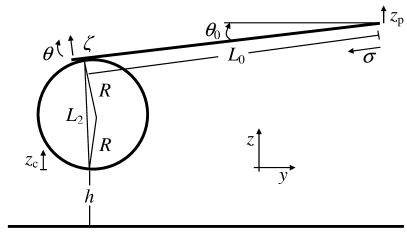
Figure 11: Cantilever geometry in the atomic force microscope (not to scale).

This analysis follows closely earlier analysis of the bending of an atomic force microscope cantilever by Attard and co-workers.Attard98 ; Attard99 ; Zhu11a ; Attard12 In turn, that analysis is based on the classical equations of continuum elasticity.Southwell36

Consider a rectangular cantilever of length $L_{0}$ and width $w\ll L_{0}$, tilted at an angle of $\theta_{0}<0$ to the horizontal with long axis in the $yz$-plane. Define $C_{0}\equiv\cos\theta_{0}$ and $S_{0}\equiv\sin\theta_{0}$. The tilt angle is small, but no linearisation will be performed. Angles are measured in a clockwise direction, and the $y$-coordinate is measured left to right. There is a spherical colloid probe of radius $R$ attached to the end of the cantilever. There is a planar substrate in the $xy$-plane located beneath the cantilever such that zero separation for the undeflected cantilever occurs when the base of the cantilever is at $z_{\mathrm{p}}=0$.

Let $\sigma\in[0,L_{0}]$ denote the running coordinate along the cantilever, with $\sigma=0$ being the base and $\sigma=L_{0}$ being the end. Note that this runs right to left, the opposite sense to the $y$-coordinate. Let $\zeta(\sigma)$ denote the deflection orthogonal to the original axis, with $\zeta_{L}\equiv\zeta(L)$ being the deflection of the end. The deflection angle is $\theta(\sigma)=\mathrm{d}\zeta(\sigma)/\mathrm{d}\sigma$, or, equivalently,

$$\zeta(\sigma)=\int_{0}^{\sigma}\mathrm{d}\sigma^{\prime}\,\theta(\sigma^{\prime}).$$ (52)

The boundary condition is $\zeta(0)=\theta(0)=0$. The deflection angle of the end, $\theta_{L}\equiv\theta(L)$, is what is measured in the atomic force microscope. The deflection will be assumed small and everything will be linearised with respect to it.

In the laboratory frame, the undeflected cantilever is described by

$$y_{0}(\sigma)=-C_{0}\sigma,\mbox{ and }z_{0}(\sigma)=z_{\mathrm{p}}+S_{0}\sigma.$$ (53)

Here $z_{\mathrm{p}}$ is the piezo-drive position, which is the location of the base of the cantilever.

The deflected cantilever has laboratory coordinates

$$y(\sigma) = -\int_{0}^{\sigma}\mathrm{d}\sigma^{\prime}\,\cos(\theta_{0}+\theta(\sigma^{\prime}))$$ (54)

$$= -C_{0}\sigma+S_{0}\int_{0}^{\sigma}\mathrm{d}\sigma^{\prime}\,\theta(\sigma^{\prime})+{\cal O}(\theta^{2})$$

$$= y_{0}(\sigma)+S_{0}\zeta(\sigma),$$

and

$$z(\sigma) = z_{\mathrm{p}}+\int_{0}^{\sigma}\mathrm{d}\sigma^{\prime}\,\sin(\theta_{0}+\theta(\sigma^{\prime}))$$ (55)

$$= z_{\mathrm{p}}+S_{0}\sigma+C_{0}\int_{0}^{\sigma}\mathrm{d}\sigma^{\prime}\,\theta(\sigma^{\prime})+{\cal O}(\theta^{2})$$

$$= z_{0}(\sigma)+C_{0}\zeta(\sigma).$$

With total angle $\theta_{\mathrm{tot}}=\theta_{0}+\theta$, a colloid probe of radius $R$ has lever arm

$$L_{2}(\theta_{\mathrm{tot}}) = R\sqrt{2+2\cos\theta_{\mathrm{tot}}}$$ (56)

$$= R\sqrt{2+2C_{0}-2S_{0}\theta+{\cal O}(\theta^{2})}$$

$$= L_{2}\left[1-\frac{S_{0}\theta}{2[1+C_{0}]}\right]+{\cal O}(\theta^{2})$$

$$= L_{2}-\frac{R^{2}S_{0}\theta}{L_{2}}+{\cal O}(\theta^{2}),$$

where $L_{2}\equiv L_{2}(\theta_{0})=R\sqrt{2+2C_{0}}$. The change in the length of the lever arm with deflection angle is small.

The change in the point of closest approach of the colloid probe (contact position) is horizontally

$$y_{\mathrm{c}} = S_{0}\zeta_{L}-L_{2}(\theta_{\mathrm{tot}})\cos(\theta_{\mathrm{tot}})\theta_{\mathrm{tot}}+L_{2}(\theta_{0})\cos(\theta_{0})\theta_{0}$$ (57)

$$= S_{0}\zeta_{L}-\left[L_{2}C_{0}-L_{2}S_{0}\theta_{0}-C_{0}\theta_{0}\frac{R^{2}S_{0}}{L_{2}}\right]\theta_{L},$$

and vertically

$$z_{\mathrm{c}} = C_{0}\zeta_{L}+\sin(\theta_{\mathrm{tot}})L_{2}(\theta_{\mathrm{tot}})\theta_{\mathrm{tot}}-S_{0}L_{2}\theta_{0}$$ (58)

$$= C_{0}\zeta_{L}+\left[S_{0}+C_{0}\theta_{0}-S_{0}\theta_{0}\frac{R^{2}S_{0}}{L_{2}^{2}}\right]L_{2}\theta_{L}$$

$$\equiv C_{0}\zeta_{L}+S_{0}^{*}L_{2}\theta_{L}.$$

These are given to linear order in the deflection and represent the change from the position of the undeflected cantilever. Note that to leading order the change in horizontal position has the opposite sign to the deflection and the deflection angle. This determines the sign of the friction force below.

The separation is

$$h=z_{\mathrm{p}}+z_{\mathrm{c}}.$$ (59)

As mentioned above, the base of the cantilever has been positioned relative to the substrate so that the undeflected cantilever is in contact when $z_{\mathrm{p}}=0$.

Let $F_{z}$ and $F_{y}$ be the components of the force acting acting on the colloid probe at the point of closest approach. The van der Waals and drainage force on the colloid probe are represented by $F_{z}$, and the friction force, when present, is represented by $F_{y}$. Typically, $F_{y}=\mu F_{z}$ in contact on extension, where $\mu$ is the friction coefficient (see the above comment regarding the sign of the change in horizontal position). These forces create a force on the end of the cantilever,

$$F_{L}=F_{z}C_{0}+F_{y}S_{0},$$ (60)

which is orthogonal to the axis of the cantilever, and a turning moment (torque),

$$M_{L}=L_{2}F_{z}S_{0}-L_{2}F_{y}C_{0},$$ (61)

which is positive in the clockwise direction. In these $\theta_{\mathrm{tot}}=\theta_{0}+\theta$ has been replaced by $\theta_{0}$ because only terms linear in the deflection are retained.

Now add a force per unit length $f(\sigma)$ in the cantilever frame (i.e. acting orthogonal to the undeflected cantilever). This is the drag (and possibly drainage) force on the cantilever, which will be given explicitly in the following section. In the cantilever frame, the turning moment about $\sigma$ due to the end force, end moment, and force per unit length is

$$M(\sigma)=[L_{0}-\sigma]F_{L}+M_{L}+\int_{\sigma}^{L_{0}}\mathrm{d}\sigma^{\prime}\,f(\sigma^{\prime})[\sigma^{\prime}-\sigma].$$ (62)

From this the deflection of the cantilever isSouthwell36

$$\zeta(\sigma) = B^{-1}\int_{0}^{\sigma}\mathrm{d}\sigma^{\prime\prime}\,M(\sigma^{\prime\prime})[\sigma-\sigma^{\prime\prime}]$$ (63)

$$= \frac{F_{L}}{B}\left[\frac{L_{0}\sigma^{2}}{2}-\frac{\sigma^{3}}{6}\right]+\frac{\sigma^{2}M_{L}}{2B}$$

$$\mbox{ }+\frac{1}{B}\int_{0}^{\sigma}\mathrm{d}\sigma^{\prime}\,f(\sigma^{\prime})\left[\frac{\sigma\sigma^{\prime}\!\,{}^{2}}{2}-\frac{\sigma^{\prime}\!\,{}^{3}}{6}\right]$$

$$\mbox{ }+\frac{1}{B}\int_{\sigma}^{L_{0}}\mathrm{d}\sigma^{\prime}\,f(\sigma^{\prime})\left[\frac{\sigma^{2}\sigma^{\prime}}{2}-\frac{\sigma^{3}}{6}\right].$$

Here $B=EI$ is the beam elasticity parameter, which is related to the intrinsic spring constant of the cantilever by $k_{0}=3B/L_{0}^{3}$.

For the case of a uniform distributed force, $f(\sigma)=f$,

$$\zeta_{L} = \frac{F_{L}}{B}\frac{L_{0}^{3}}{3}+\frac{L_{0}^{2}M_{L}}{2B}+\frac{f}{B}\left[\frac{L_{0}^{4}}{6}-\frac{L_{0}^{4}}{24}\right]$$ (64)

$$= \frac{F_{L}}{k_{0}}+\frac{3M_{L}}{2L_{0}k_{0}}+\frac{3L_{0}f}{8k_{0}}.$$

For the case that there is no drag or drainage force on the cantilever, $f(\sigma)=0$, the end deflection is

$$\zeta_{L}=\frac{F_{L}}{k_{0}}+\frac{3M_{L}}{2L_{0}k_{0}}.$$ (65)

If in addition there is no lever arm, $L_{2}=M_{L}=0$, nor friction force, $F_{y}=0$, so that the end force is $F_{L}=F_{z}C_{0}$, then the end deflection reduces to

$$\zeta_{L}=\frac{F_{z}C_{0}}{k_{0}},\mbox{ or }z_{\mathrm{c}}=\frac{F_{z}C_{0}^{2}}{k_{0}}.$$ (66)

Here $\zeta_{L}C_{0}$ is the vertical deflection of the end of the cantilever in the laboratory frame. In this case with no lever arm, $L_{2}=0$, the vertical deflection of the end is the same as the change in vertical position of the contact point, $z_{\mathrm{c}}=\zeta_{L}C_{0}$.

This result does not agree with the result given by Vinogradova and YakubovVinogradova03 for the same case (their Eq. (6), in the present notation, is $z_{\mathrm{c}}={F_{z}}[3C_{0}-1]/{2k_{0}}$). In the opinion of the present author, the error in Ref. Vinogradova03, arises in the very first equation where the authors mix up the internal coordinates of the cantilever with the laboratory coordinates. Consequently, the present author believes that all of the results in Ref. Vinogradova03, are suspect.

From the general expression for the deflection of the cantilever, the angular deflection of the end, $\theta_{L}=\left.\mathrm{d}\zeta(\sigma)/\mathrm{d}\sigma\right|_{\sigma=L_{0}}$, is

$$\theta_{L}=\frac{L_{0}^{2}F_{L}}{2B}+\frac{L_{0}M_{L}}{B}+\frac{1}{B}\int_{0}^{L_{0}}\mathrm{d}\sigma^{\prime}\,f(\sigma^{\prime})\frac{\sigma^{\prime}\!\,{}^{2}}{2}.$$ (67)

This is important because it is what is actually measured in the atomic force microscope. For the case of a uniform force per unit length, $f(\sigma)=f$, this reduces to

$$\theta_{L}=\frac{L_{0}^{2}F_{L}}{2B}+\frac{L_{0}M_{L}}{B}+\frac{L_{0}^{3}f}{6B}.$$ (68)

In the case of only probe forces, (i.e. no distributed drag or drainage forces on the cantilever), a number of useful constants can be given. First define for convenience

$$C_{+}\equiv C_{0}+\tilde{\mu}S_{0}\mbox{ and }S_{-}\equiv S_{0}-\tilde{\mu}C_{0},$$ (69)

which differ from $C_{0}$ and $S_{0}$ only in contact since the effective friction coefficient is defined as

$$\tilde{\mu}=\left\{\begin{array}[]{ll}\mu,&\mbox{contact, extension},\\ -\mu,&\mbox{contact, retraction},\\ 0,&\mbox{non-contact}.\end{array}\right.$$ (70)

With these, the ratio of the end deflection to the surface force is

$$\frac{\zeta_{L}}{F_{z}}=\frac{C_{+}}{k_{0}}+\frac{3L_{2}S_{-}}{2L_{0}k_{0}},$$ (71)

and the ratio of the angle deflection to the surface force is

$$\frac{\theta_{L}}{F_{z}}=\frac{3C_{+}}{2L_{0}k_{0}}+\frac{3L_{2}S_{-}}{L_{0}^{2}k_{0}}.$$ (72)

Using these, the effective spring constant, which is defined as the ratio of the vertical force to the vertical contact point deflection, is

$$k_{\mathrm{eff}}(\tilde{\mu})\equiv\frac{F_{z}}{z_{\mathrm{c}}}$$

$$= \frac{F_{z}}{C_{0}\zeta_{L}+S_{0}^{*}L_{2}\theta_{L}}$$

$$= \frac{k_{0}}{C_{0}\left[C_{+}+\frac{3L_{2}S_{-}}{2L_{0}}\right]+S_{0}^{*}L_{2}\left[\frac{3C_{+}}{2L_{0}}+\frac{3L_{2}S_{-}}{L_{0}^{2}}\right]}.$$

When one speaks of ‘the’ effective spring constant, one means out of contact, $k_{\mathrm{eff}}\equiv k_{\mathrm{eff}}(0)$, (which means $C_{+}=C_{0}$, $S_{-}=S_{0}$). One can see that for the case $L_{2}=0$, which means that $z_{\mathrm{c}}=C_{0}\zeta_{L}$, this is the same as Eq. (66). These expression agree with those given in §§B.9 and B.10.

These three equations are sufficient to obtain everything that is needed from an atomic force measurement of surface forces that has been analysed to give the angular deflection. That is, they give $F_{z}(\theta_{L})$, and hence $z_{\mathrm{c}}(F_{z})$, and hence $h=z_{\mathrm{p}}-z_{\mathrm{c}}(F_{z})+z_{0}$. This assumes that the the angular deflection and the zero of separation have been obtained as described in §B. It also assumes that any variation in distributed forces on the cantilever can be neglected, which means that these are apparent rather than real quantities.

C.4 Drag Force on Cantilever

In the atomic force microscope one measures a drag force at large separations

$$F_{\mathrm{drag}}=-6\pi\eta L_{\mathrm{drag}}\dot{z}_{\mathrm{p}}.$$ (74)

This defines the drag parameter $L_{\mathrm{drag}}$. The drag length is an effective quantity that accounts for the cantilever shape, the fact that the drive velocity is not orthogonal to the cantilever axis, (if one wanted to, one could instead define $F_{\mathrm{drag}}=-6\pi\eta\tilde{L}_{\mathrm{drag}}C_{0}\dot{z}_{\mathrm{p}}$, with $\tilde{L}_{\mathrm{drag}}=L_{\mathrm{drag}}/C_{0}$), and, most importantly, the fact that the distributed drag force is interpreted as if it were a point force on the contact point.

The drag force per unit length may be taken to be

$$f(\sigma)=-c_{\mathrm{drag}}[\dot{z}_{\mathrm{p}}C_{0}+\dot{\zeta}(\sigma)].$$ (75)

This simply says that the local drag force is proportional to the local velocity of the cantilever through the liquid. This drag force is orthogonal to the axis of the undeflected cantilever, which was how the distributed force was defined.

At large separations $\dot{\zeta}(\sigma)\approx 0$ and this force is uniform. In this case, Eq. (68) gives the deflection angle as

$$\theta_{L}=\frac{-c_{\mathrm{drag}}\dot{z}_{\mathrm{p}}C_{0}}{2k_{0}}.$$ (76)

The end force and moment due to a point force, $F_{z}=F_{\mathrm{drag}}$, and no friction, $F_{y}=0$, is $F_{L}=C_{0}F_{\mathrm{drag}}$ and $M_{L}=L_{2}S_{0}F_{\mathrm{drag}}$, which gives a deflection angle

$$\theta_{L}=\left[\frac{3C_{0}}{2L_{0}k_{0}}+\frac{3L_{2}S_{0}}{L_{0}^{2}k_{0}}\right]F_{\mathrm{drag}}.$$ (77)

Equating these two expressions for the deflection angle gives

$$c_{\mathrm{drag}} = \frac{2k_{0}}{\dot{z}_{\mathrm{p}}C_{0}}\left[\frac{3C_{0}}{2L_{0}k_{0}}+\frac{3L_{2}S_{0}}{L_{0}^{2}k_{0}}\right]6\pi\eta L_{\mathrm{drag}}\dot{z}_{\mathrm{p}}$$ (78)

$$= \frac{12\pi\eta L_{\mathrm{drag}}}{C_{0}}\left[\frac{3C_{0}}{2L_{0}}+\frac{3L_{2}S_{0}}{L_{0}^{2}}\right].$$

The leading term is identical to that used previously.Zhu11a (Previously the subordinate term due to tilt and torque were not accounted for.)

C.5 Comparison of Theory and Measurement

Next an algorithm will be given for computing the deflection of the cantilever due to the drainage and van der Waals forces on the colloid probe and the drag force on the cantilever. This algorithm gives the actual vertical deflection $z_{\mathrm{c}}$, the actual separation $h$, and the actual surface force $F_{z}$, as well as the actual angular deflection $\theta_{L}$. The atomic force microscope measures $\theta_{L}$, and assumes that this angular deflection is due solely to a point force $F_{z}$, and uses the point force equations to convert the angular deflection to an apparent vertical deflection, an apparent separation, and an apparent point force. This procedure would be accurate if the distributed drag force on the cantilever were constant, (because then the distributed force contribution to the deflection is just a constant that is removed in the base line treatment of the data). However to the extent that the drag force is varying with cantilever deflection, the apparent quantities are not equal to the actual quantities. Therefore, in comparing theory with measurement one has to convert an exact angular deflection given by theory to an apparent vertical deflection, an apparent separation, and an apparent point force, using the same conversion factors that one uses to analyze the atomic force microscope raw data. (Out of interest, one can always compare the actual and the apparent calculated quantities to see how big an effect variable drag has.) In the text above, it is the apparent theoretical and experimental quantities that are plotted.

C.6 Numerical Computation for Variable Drag

The shape of the cantilever $\zeta(\sigma)$ under the influence of the point and distributed forces was given above as Eq. (63). The shape is a function $F_{z}$ (via the friction force $F_{y}$, if present, the end force $F_{L}$, and the end moment $M_{L}$), which gives it a direct dependence on $h$ and $\dot{h}$, and a functional of $\dot{\zeta}(\sigma)$ (via $f(\sigma)$). This function will be denoted $S(\sigma;F_{z},[\zeta])$, or more simply $S(\sigma)$. (This is necessary because in the numerical solution of the equations of motion, one has to distinguish and to equate the shape that evolves from the previous shape, $\zeta(t+\Delta_{t})$, and the shape that satisfies the elasticity equation, $S(\sigma(t+\Delta_{t}))$.) The deflection of the end for a given shape is $\zeta_{L}\equiv\zeta(L_{0})=S(L_{0})$. Similarly the deflection angle of the end is $\theta_{L}=\left.\mathrm{d}S(\sigma)/\mathrm{d}\sigma\right|_{\sigma=L_{0}}$. The separation is $h=z_{\mathrm{p}}+z_{\mathrm{c}}$, and the rate of change of separation is $\dot{h}=\dot{z}_{\mathrm{p}}+\dot{z}_{\mathrm{c}}$, where $z_{\mathrm{c}}$ is the function of $\zeta_{L}$ and $\theta_{L}$ given above, Eq. (58). For convenience the constant of separation has been chosen as zero.

The problem to be solved is: given the drive trajectory $z_{\mathrm{p}}(t)$, at each instant calculate the shape $S(\sigma;t)$ and hence $\zeta_{L}(t)$, $\theta_{L}(t)$, $h(t)$ etc. The axial coordinate can be discretised, $\sigma_{i}=i\Delta_{\sigma}$ and the shape can be written simply as a vector ${\bm{\zeta}}$, with elements $\zeta_{i}=\zeta(\sigma_{i})$. Also $i\in[0,L]$, $\sigma_{L}=L_{0}$ and $\zeta_{L}=\zeta(y_{L})=\zeta(L_{0})$, consistent with the notation introduced above.

Suppose the shape ${\bm{\zeta}}$ and its rate of change $\dot{\bm{\zeta}}$ is known at time $t$. It is required to obtain these at time $t^{\prime}=t+\Delta_{t}$. One has three equations to solve:

$${\bm{\zeta}}^{\prime} = {\bm{\zeta}}+\Delta_{t}\dot{\bm{\zeta}}+\frac{1}{2}\Delta_{t}^{2}\ddot{\bm{\zeta}},$$

$$\dot{\bm{\zeta}}^{\prime} = \dot{\bm{\zeta}}+\Delta_{t}\ddot{\bm{\zeta}},$$

$${\bm{\zeta}}^{\prime} = {\bf S}(F_{z}^{\prime},\dot{\bm{\zeta}}^{\prime}).$$ (79)

Clearly then one has a single unknown vector, namely the acceleration $\ddot{\bm{\zeta}}$, and one can insert the first two equations into the third, which can then be written as a function of the acceleration, ${\bm{\zeta}}^{\prime}(\ddot{\bm{\zeta}})={\bf S}(\ddot{\bm{\zeta}})$. (Both sides of this depend upon the known ${\bm{\zeta}}$ and $\dot{\bm{\zeta}}$ at the preceding time step.) Equivalently then one has to find the zero of the vector function

$${\bf G}(\ddot{\bm{\zeta}})\equiv{\bm{\zeta}}^{\prime}(\ddot{\bm{\zeta}})-{\bf S}(\ddot{\bm{\zeta}}).$$ (80)

In order to develop a stable iteration procedure to solve this, one converts it to a fixed point problem and uses essentially Newton’s method. That is, define

$${\bf H}(\ddot{\bm{\zeta}})\equiv\ddot{\bm{\zeta}}-\left(\frac{\partial{\bf G}}{\partial\ddot{\bm{\zeta}}}\right)^{-1}{\bf G}(\ddot{\bm{\zeta}}),$$ (81)

where the Jacobean matrix has elements $\left\{{\partial{\bf G}}/{\partial\ddot{\bm{\zeta}}}\right\}_{ij}={\partial G_{i}}/{\partial\ddot{\zeta}_{j}}$. Clearly the correct acceleration $\overline{\ddot{\bm{\zeta}}}$, which satisfies ${\bf G}(\overline{\ddot{\bm{\zeta}}})={\bf 0}$ is a fixed point of this, ${\bf H}(\overline{\ddot{\bm{\zeta}}})=\overline{\ddot{\bm{\zeta}}}$. Hence one can set up an iteration procedure for the acceleration,

$$\ddot{\bm{\zeta}}^{(n+1)}={\bf H}(\ddot{\bm{\zeta}}^{(n)}).$$ (82)

The procedure has been designed to be quadratically convergent by making the Jacobean of ${\bf H}$ vanish at the fixed point. To avoid matrix inversion, this is more conveniently written

$$\frac{\partial{\bf G}^{(n)}}{\partial\ddot{\bm{\zeta}}}\;\ddot{\bm{\zeta}}^{(n+1)}=\frac{\partial{\bf G}^{(n)}}{\partial\ddot{\bm{\zeta}}}\;\ddot{\bm{\zeta}}^{(n)}-{\bf G}^{(n)}.$$ (83)

Care has to be taken with the matrix multiplications, since these should be weighted according to the trapezoidal quadrature rule. Gaussean elimination can be used to obtain from this the next iterate for the acceleration. For the first guess, the converged acceleration from the preceding time step can be used, $\ddot{\bm{\zeta}}^{(0)}(t^{\prime})=\ddot{\bm{\zeta}}(t)$.

The elements of the Jacobean matrix are explicitly

$$\frac{\partial G_{i}}{\partial\ddot{\zeta}_{j}}=\frac{\Delta_{t}^{2}}{2}\delta_{ij}-\frac{\partial S_{i}^{\prime}}{\partial F_{z}^{\prime}}\frac{\partial F_{z}^{\prime}}{\partial\ddot{\zeta}_{j}}-\Delta_{t}\frac{\partial S_{i}}{\partial\dot{\zeta}_{j}}.$$ (84)

with $F_{z}^{\prime}=F_{z}(t+\Delta_{t})$. A Kronecker-$\delta$ appears here. One has

$$\frac{\partial S_{i}}{\partial\dot{\zeta}_{j}} = \frac{-\Delta_{\sigma}c_{\mathrm{drag}}/B}{1+\delta_{j0}+\delta_{jL}}\times\left\{\begin{array}[]{ll}\displaystyle\frac{\sigma_{i}\sigma_{j}^{2}}{2}-\frac{\sigma_{j}^{3}}{6}&j\leq i,\\ \displaystyle\rule{0.0pt}{17.07182pt}\frac{\sigma_{i}^{2}\sigma_{j}}{2}-\frac{\sigma_{i}^{3}}{6},&j\geq i,\end{array}\right.$$ (87)

and

$$\frac{\partial S_{i}}{\partial F_{z}}=B^{-1}\left[\frac{1}{2}L_{0}\sigma_{i}^{2}-\frac{1}{6}\sigma_{i}^{3}\right]\frac{\partial F_{L}}{\partial F_{z}}+\frac{y_{i}^{2}}{2B}\frac{\partial M_{L}}{\partial F_{z}}.$$ (88)

In turn one has

$$\frac{\partial F_{L}}{\partial F_{z}}=C_{0}+\tilde{\mu}S_{0},\mbox{ and }\frac{\partial M_{L}}{\partial F_{z}}=L_{2}S_{0}-\tilde{\mu}L_{2}C_{0},$$ (89)

where the effective friction constant was given above. Finally,

$$\frac{\partial F_{z}^{\prime}}{\partial\ddot{\zeta}_{j}} = \frac{\partial F_{z}}{\partial h}\frac{\partial z_{\mathrm{c}}^{\prime}}{\partial\ddot{\zeta}_{j}}+\frac{\partial F_{z}}{\partial\dot{h}}\frac{\partial\dot{z}_{\mathrm{c}}^{\prime}}{\partial\ddot{\zeta}_{j}}$$ (90)

$$= \left[\frac{\Delta_{t}^{2}}{2}\frac{\partial F_{z}}{\partial h}+\Delta_{t}\frac{\partial F_{z}}{\partial\dot{h}}\right]\left[C_{0}\frac{\partial\zeta_{L}}{\partial\zeta_{j}}+S_{0}^{*}L_{2}\frac{\partial\theta_{L}}{\partial\zeta_{j}}\right]$$

$$= \left[\frac{\Delta_{t}^{2}}{2}\frac{\partial F_{z}}{\partial h}+\Delta_{t}\frac{\partial F_{z}}{\partial\dot{h}}\right]$$

$$\mbox{ }\times\left[C_{0}\delta_{Lj}+\frac{S_{0}^{*}L_{2}}{\Delta_{\sigma}}\left\{\delta_{Lj}-\delta_{L-1,j}\right\}\right].$$

The final term follows because the deflection angle of the end is $\theta_{L}\equiv[\zeta_{L}-\zeta_{L-1}]/\Delta_{\sigma}$. The force derivatives were given in §C.2.

Typically $L=100$ points were used to discretise the axial integrals. This many points markedly slows the Gaussean elimination. Therefore an orthonomal basis for a sub-space was constructed, $\underline{v}_{n}$, with $n=1,2,\ldots$, with elements $v_{ni}$ a polynomial in $y_{i}$ of degree $n$. The polynomials are chosen orthogonal on the interval $[0,L_{0}]$ with trapezoidal weighting. The orthonomal basis was constructed numerically. Typically four vectors were used for the basis. The various matrices and vectors were projected onto the sub-space and the iteration for the acceleration carried out. Typically 5 iterations were used at each time step. Tests showed the results did not change upon increasing the number of iterations, basis vectors, or grid points. The procedure was found to be quite stable. This includes in contact, the turn around point, and the jump from contact.

C.7 Simplified Algorithm for Constant Drag

The algorithm simplifies considerably if one can neglect the variation in cantilever drag with deflection. In this case one only needs the vertical deflection $z_{\mathrm{c}}$, the velocity, $\dot{z}_{\mathrm{c}}$, and the acceleration $\ddot{z}_{\mathrm{c}}$ of the contact point. With again $t^{\prime}=t+\Delta_{t}$, the three equations to be solved are

$$z_{\mathrm{c}}^{\prime} = z_{\mathrm{c}}+\Delta_{t}\dot{z}_{\mathrm{c}}+\frac{1}{2}\Delta_{t}^{2}\ddot{z}_{\mathrm{c}},$$

$$\dot{z}_{\mathrm{c}}^{\prime} = \dot{z}_{\mathrm{c}}+\Delta_{t}\ddot{z}_{\mathrm{c}},$$

$$z_{\mathrm{c}}^{\prime} = F_{z}(h^{\prime},\dot{h}^{\prime})/k_{\mathrm{eff}}.$$ (91)

Recall $F_{z}\equiv F_{\mathrm{vdW}}+F_{\mathrm{drain}}$. Because $h^{\prime}=z_{\mathrm{p}}^{\prime}+z_{\mathrm{c}}^{\prime}$, the right hand side of the last equation is a function of $\ddot{z}_{\mathrm{c}}$. Hence the correct acceleration is the zero of

$$G(\ddot{z}_{\mathrm{c}})\equiv z_{\mathrm{c}}^{\prime}(\ddot{z}_{\mathrm{c}})-F_{z}(h^{\prime},\dot{h}^{\prime})/k_{\mathrm{eff}}.$$ (92)

This is converted into a fixed point problem by defining

$$H(\ddot{z}_{\mathrm{c}}) \equiv \ddot{z}_{\mathrm{c}}-\left(\frac{\partial G}{\partial\ddot{z}_{\mathrm{c}}}\right)^{-1}G(\ddot{z}_{\mathrm{c}})$$

$$= \ddot{z}_{\mathrm{c}}-\frac{z_{\mathrm{c}}+\Delta_{t}\dot{z}_{\mathrm{c}}+0.5\Delta_{t}^{2}\ddot{z}_{\mathrm{c}}-F_{z}(h^{\prime},\dot{h}^{\prime})/k_{\mathrm{eff}}}{\displaystyle\frac{\Delta_{t}^{2}}{2}-\frac{\partial F_{z}(h^{\prime},\dot{h}^{\prime})}{k_{\mathrm{eff}}\partial h^{\prime}}\frac{\Delta_{t}^{2}}{2}-\frac{\partial F_{z}(h^{\prime},\dot{h}^{\prime})}{k_{\mathrm{eff}}\partial\dot{h}^{\prime}}\Delta_{t}}.$$

From this, the iteration procedure for the acceleration is

$$\ddot{z}_{\mathrm{c}}^{(n+1)}=H(\ddot{z}_{\mathrm{c}}^{(n)}).$$ (94)

This is quadratically convergent and was found to be quite stable, including in the contact region where the van der Waals force is steeply repulsive.

References

- (1) Neto, C., Evans, D. R., Bonaccurso, E., Butt, H. J., and Craig, V. S. J. (2005), Rep. Prog. Phys. 68, 2859.
- (2) Bocquet, L. and Charlaix, E. (2010), Chem. Soc. Rev. 39, 1073.
- (3) Zhu, L., Attard, P., and Neto, C. (2012), Langmuir, 28, 7768.
- (4) Attard, P. (2012), arXiv:1212.3019v2 .
- (5) Zhu, L., Attard, P., and Neto, C. (2011), Langmuir, 27, 6701.
- (6) Zhu, L., Attard, P., and Neto, C. (2011), Langmuir, 27, 6712.
- (7) Zhu, L., Neto, C. and Attard, P. (2012), Langmuir, 28, 3465.
- (8) Craig, V. S. J. and Neto, C. (2001), Langmuir 17, 6018.
- (9) Attard, P., Pettersson, T., and Rutland, M. W. (2006), Rev. Sci. Instrum. 77, 116110.
- (10) Higgins, J., Proksch, R., Sader, J. E., Polcik, M., McEndoo, S., Cleveland, J. P., and Jarvis, S. P. (2006), Rev. Sci. Instrum. 77, 013701 .
- (11) Attard, P., Schulz, J., and Rutland, M. W. (1998), Rev. Sci. Instrum. 69, 3852.
- (12) Attard, P., Carambassis, A., and Rutland, M. W. (1999), Langmuir 15, 553.
- (13) Vinogradova, O. I. (1995), Langmuir, 11, 2213.
- (14) Attard P. and Parker J. L. (1992), Phys. Rev. A 46, 7959. Erratum, (1994) Phys. Rev. E 50, 5145.
- (15) Southwell, R. V. (1936), An Introduction to the Theory of Elasticity, (Oxford, London).
- (16) Vinogradova, O. I. and Yakubov, G. E. (2003), Langmuir, 19, 1227.