The evolution of H i and C iv quasar absorption line systems at $1.9<z<3.2$

We have investigated the distribution and evolution of $\sim$3100 intergalactic neutral hydrogen (H i) absorbers with H i column densities $\log N_{\mathrm{{H\textsc{i}}}}\!=\![12.75,17.0]$ at $1.9\!<\!z\!<\!3.2$, using 18 high resolution, high signal-to-noise quasar spectra obtained from the ESO VLT/UVES archive. We used two sets of Voigt profile fitting analysis, one including all the available high-order Lyman lines to obtain reliable H i column densities of saturated lines, and another using only the Ly$\alpha$ transition. There is no significant difference between the Ly$\alpha$-only fit and the high-order Lyman fit results. Combining our Ly$\alpha$-only fit results at $1.7\!<\!z\!<\!3.6$ with high-quality literature data, the mean number density at $0<z<4$ is not well described by a single power law and strongly suggests that its evolution slows down at $z\leq 1.5$ at the high and low column density ranges. We also divided our entire H i absorbers at $1.9\!<\!z\!<\!3.2$ into two samples, the unenriched forest and the C iv-enriched forest, depending on whether H i lines are associated with C iv at $\log N_{\mathrm{{C\textsc{iv}}}}\!\geq\!12.2$ within a given velocity range. The entire H i column density distribution function (CDDF) can be described as the combination of these two well-characterised populations which overlap at $\log N_{\mathrm{{H\textsc{i}}}}\sim 15$. At $\log N_{\mathrm{{H\textsc{i}}}}\leq 15$, the unenriched forest dominates, showing a similar power-law distribution to the entire forest. The C iv-enriched forest dominates at $\log N_{\mathrm{{H\textsc{i}}}}\geq 15$, with its distribution function as $\propto N_{\mathrm{{H\textsc{i}}}}^{\sim-1.45}$. However, it starts to flatten out at lower $N_{\mathrm{{H\textsc{i}}}}$, since the enriched forest fraction decreases with decreasing $N_{\mathrm{{H\textsc{i}}}}$. The deviation from the power law at $\log N_{\mathrm{{H\textsc{i}}}}=[14,17]$ shown in the CDDF for the entire H i sample is a result of combining two different H i populations with a different CDDF shape. The total H i mass density relative to the critical density is $\Omega_{\mathrm{{H\textsc{i}}}}\sim 1.6\times 10^{-6}h^{-1}$, where the enriched forest accounts for $\sim 40$% of $\Omega_{\mathrm{{H\textsc{i}}}}$.

1 Introduction

The resonant Ly$\alpha$ absorption by neutral hydrogen (H i) in the warm ($\sim 10^{4}$ K) photoionised intergalactic medium (IGM) produces rich absorption features blueward of the Ly$\alpha$ emission line in high-redshift quasar spectra known as the Ly$\alpha$ forest. The Ly$\alpha$ forest contains $\sim\!90$% of the baryonic matter at $z\!\sim\!3$ and can be observed in a wide range of redshifts up to $z\!\sim\!6$. Gas-dynamical simulations and semi-analytic models have been very successful at explaining the observed properties of the Ly$\alpha$ forest mainly at low H i column densities $N_{\mathrm{{H\textsc{i}}}}\leq 10^{16}$ cm^-2. These models have shown that the Ly$\alpha$ forest arises by mildly non-linear density fluctuations in the low-density H i gas, which follows the underlying dark matter distribution on large scales. This interpretation also predicts that the Ly$\alpha$ forest provides powerful observational constraints on the distribution and evolution of the baryonic matter in the Universe, hence the evolution of galaxies and the large-scale structure (Cen et al. 1994; Rauch et al. 1997; Theuns et al. 1998; Davé et al. 1999; Schaye et al. 2000b; Schaye 2001; Kim et al. 2002). In addition, the discovery of triply ionised carbon (C iv) associated with some of the forest absorbers suggests that the forest metal abundances can be utilised to probe early generations of star formation and the feedback between high-redshift galaxies and the surrounding IGM from which galaxies formed (Cowie et al. 1995; Davé et al. 1998; Aguirre et al. 2001; Schaye et al. 2003; Oppenheimer & Davé 2006).

The physics of the Ly$\alpha$ forest is mainly governed by three competing processes, the Hubble expansion, the gravitational growth and the ionizing UV background radiation. The Hubble expansion which causes the gas to cool adiabatically and the gravitational growth are fairly well-constrained by the cosmological parameters and the primordial power spectrum from the latest WMAP observations (Jarosik et al. 2011). On the other hand, the ionizing UV background radiation controls the photoionisation heating and the gas ionisation fraction, thus determining the fraction of the observable H i gas compared to the unobservable H ii gas. The UV background is assumed to be provided primarily by quasars and in some degree also by star-forming galaxies (Shapley et al. 2006; Siana et al. 2010) and Ly$\alpha$ emitters (Iwata et al. 2009). However, the intensity/spectral shape of the UV background and the relative contribution from quasars and galaxies as a function of redshift are not well constrained (Bolton et al. 2005; Faucher-Giguère et al. 2008). One of the common methods to measure the UV background and its evolution is the quasar proximity effect (Dall’Aglio et al. 2008). Unfortunately, measurements of the UV background through the proximity effect are biased by the large scale density distribution around the quasars which cannot be easily quantified observationally (Partl et al. 2010, 2011).

Two commonly explored quantities to constrain the properties of the Ly$\alpha$ forest are the number of absorbers for a given H i column density range per unit redshift, $\mathrm{d}n/\mathrm{d}z$, and the differential column density distribution function (CDDF, the number of absorbers per unit absorption path length and per unit column density, an analogue to the galaxy luminosity function). Compared with simulations, detailed structures seen in an overall power-law-like CDDF ($\propto N_{\mathrm{{H\textsc{i}}}}^{\beta}$) such as a flattening or a steepening at different column density ranges constrain various forest physical and galactic feedback processes (Altay et al. 2011; Davé et al. 2010). The CDDF is also one of the main observables required in calculating the mass density relative to the critical density contributed by the forest (Schaye 2001). The shape of the CDDF at lower $N_{\mathrm{{H\textsc{i}}}}\leq 10^{12.5-12.7}$ cm s^-2 (a typical detection limit for most available high-quality data) is of particular importance, since the lower $N_{\mathrm{{H\textsc{i}}}}$ absorbers are much more numerous than higher $N_{\mathrm{{H\textsc{i}}}}$ absorbers, thus they can trace a significant fraction of baryons, depending on the steepness of the CCDF at the low $N_{\mathrm{{H\textsc{i}}}}$ limit.

On the other hand, $\mathrm{d}n/\mathrm{d}z$ provides an additional way to study the UV background radiation and its evolution. The gas density decreases with decreasing redshift due to the Hubble expansion. A lower gas density results in a strong reduction of the recombination rate, allowing the gas to settle in to a photoionisation equilibrium with a higher ionisation fraction. With the non-decreasing background radiation, this causes a steep number density evolution. However, the decrease of the quasar number density at $z\!<\!2.5$ also decreases the available ionising photons (Silverman et al. 2005). This changes the ionisation fraction in the gas and also counteracts the gas density decrease, and hence slows down the number density evolution (Theuns et al. 1998; Davé et al. 1999; Bianchi et al. 2001).

The result from the HST/FOS Quasar Absorption Line Key project shows such a slow change in the $\mathrm{d}n/\mathrm{d}z$ evolution at $z\!<\!1.5$ (Weymann et al. 1998), compared to a much steeper $\mathrm{d}n/\mathrm{d}z$ evolution shown at $z\!>\!2$ (Kim et al. 1997, 2001, 2002). Cosmic variance also seems to increase at lower $z$ (Kim et al. 2002). Unfortunately, recent work based on better-quality HST data at $z\!<\!1.5$ (or the observed H i Ly$\alpha$ at $<\!3050$ Å) have shown rather ambiguous $\mathrm{d}n/\mathrm{d}z$ results with a large scatter along different sightlines (Janknecht et al. 2006; Lehner et al. 2007; Williger et al. 2010). The only certain observational fact is that all of these newer studies show a factor of $\sim 2-3$ lower number densities than the Weymann et al. values at $z\!<\!1.5$. Considering a lack of results from good-quality data at $1\!<\!z\!<\!1.5$ in the literature, the redshift evolution of $\mathrm{d}n/\mathrm{d}z$ can be considered as a single power law without any abrupt change in $\mathrm{d}n/\mathrm{d}z$ at $0\!<\!z\!<\!3.5$.

Here we present an in-depth Voigt profile fitting analysis of 18 high resolution ($R\!\sim\!45\,000$), high signal-to-noise ($\sim\!35$–50 per pixel) quasar spectra obtained with the UVES (Ultra-violet Visible Echelle Spectrograph) on the VLT, covering the Ly$\alpha$ forest at $1.9\!<\!z_{\mathrm{forest}}\!<\!3.2$. Our main scientific aims are to derive the redshift evolution of the absorber number density and the column density distribution function from a large and homogeneous set of data available at $z\!>\!2$, since most previous high-quality forest studies at $z\!>\!2$ have been based on less than 5 sightlines. Even with few sightlines, the statistics for the weak forest lines is robust due to the large number of weak absorbers with $N_{\mathrm{{H\textsc{i}}}}\!=\!10^{13-15}$ cm^-2 (about 150 absorbers at $z\!\sim\!2.5$ per sightline, i.e. in the wavelength range between the quasar’s Ly$\alpha$ and Ly$\beta$ emission lines). However, for the stronger forest systems with $N_{\mathrm{{H\textsc{i}}}}\!\geq\!10^{15}$ cm^-2, more sightlines are required since there are only about 10 absorbers per sightline at $z\!\sim\!2.5$. Cosmic variance also plays an important role at lower redshifts, especially for stronger absorbers (Kim et al. 2002). Therefore, increasing the sample size at $z\!\sim\!2$ is critical in addressing the $N_{\mathrm{{H\textsc{i}}}}$ evolution for the Ly$\alpha$ forest.

In addition to the increased sample size, we have improved previous results in two ways. First, most previous studies on the forest from ground-based observations at $z>1.7$ have been based on the Ly$\alpha$-only profile fitting analysis. This approach does not provide a reliable $N_{\mathrm{{H\textsc{i}}}}$ for saturated lines, $N_{\mathrm{{H\textsc{i}}}}\!\geq\!10^{14.5}$ cm^-2 for the present UVES data. To derive a more reliable $N_{\mathrm{{H\textsc{i}}}}$ of saturated lines, we have included all the available high-order Lyman series in this study.

Second, strong evidence have been accumulated in recent studies that metals associated with the high-redshift Ly$\alpha$ forest are within $\sim\!100$ kpc of galaxies as in the circum-galactic medium rather than in the intergalactic space far away from galaxies (Adelberger et al. 2005; Steidel et al. 2010; Rudie et al. 2012). This implies that the H i absorbers containing metals might show different properties than the ones without detectable metals. Taking C iv as a metal proxy, we have divided our data into two samples, one with C iv (the C iv-enriched forest) and another without C iv (the unenriched forest), in order to test this scenario of the circum-galactic medium. Since our study lacks the imaging survey around the quasar targets, we cannot claim that the C iv-enriched forest is indeed located within $\sim\!100$ kpc from a nearby galaxy. However, this study provides complementary results to galaxy-absorber connection studies at high redshifts (Steidel et al. 2010; Rudie et al. 2012).

This study is also very timely since the Cosmic Origins Spectrograph (COS), a high-sensitivity FUV spectrograph onboard HST has started to produce many high-quality quasar spectra at $z<1$ (Green et al. 2012; Savage et al. 2012). These COS quasar observations have opened a new tool to study the low-$z$ Ly$\alpha$ forest. Combined with results at high redshifts such as our study, COS observations will make it possible to characterise the $\mathrm{d}n/\mathrm{d}z$ evolution at $0\!<\!z\!<\!3.5$ in a more robust way, thus a stringent constraint on the UV background evolution.

This paper is organised as follows. Section 2 describes the analysed data and two Voigt profile fitting methods. Comparisons with previous studies based on the Ly$\alpha$-only fit are shown in Section 3. The analysis based on the high-order Lyman fit is presented in Section 4. Column density distribution and evolution of the Ly$\alpha$ forest containing C iv are presented in Section 5. Finally, we discuss and summarise the main results in Section 6. All the results on the number density and the differential column density distribution from our analysis are tabulated in Appendix A. Throughout this study, the cosmological parameters are assumed to be the matter density $\Omega_{m}=0.3$, the cosmological constant $\Omega_{\Lambda}=0.7$ and the current Hubble constant $H_{\mathrm{0}}=100h$ km s^-1 Mpc^-1 with $h=0.7$, which is in concordance with latest WMAP measurements (Jarosik et al. 2011). The logarithm $N_{\mathrm{{H\textsc{i}}}}$ is defined as $\log N_{\mathrm{{H\textsc{i}}}}=\log(N_{\mathrm{{H\textsc{i}}}}/1\,\,\mathrm{cm}^{-2})$.

Table 1: Analysed quasars

Quasar	$z_{\mathrm{em}}$	$z_{\mathrm{Ly\alpha}}^{\mathrm{a}}$	$z_{\mathrm{Ly\alpha\beta}}^{\mathrm{b}}$	$z_{\mathrm{Ly,high-order}}^{\mathrm{c}}$	Excluded $z_{\mathrm{{C\textsc{iv}}}}^{\mathrm{d}}$	S/N per pixele	LL (Å)	notes
Q0055–269	3.655f	2.936–3.605		2.936–3.205	not used	50–80 […, …]	2288
PKS2126–158	3.279	2.815–3.205		2.815–3.205		50–200 […, 170]	3457	two sub-DLAs at $z=$2.768 & 2.638
Q0420–388	3.116f	2.480–3.038	2.665–3.038	2.665–3.038	2.607–2.670	100–140 […, 120]	3754	a sub-DLA at $z=$3.087
HE0940–1050	3.078	2.452–3.006			2.714–2.778	50–130 […, 115]	$\leq 3200$
HE2347–4342	2.874f	2.336–2.819			2.708–2.773	100–160 [105, 120]	$\leq 1160$	multiple associated systems
Q0002–422	2.767	2.209–2.705				60–70 [140, 170]	3025
PKS0329–255	2.704f	2.138–2.651				40–60 [90, 90]	3157	an associated system at 4513.7 Å
Q0453–423	2.658f	2.359–2.588				90–100 [130, 120]	3022	a sub-DLA at $z=$2.305
		2.091–2.217
HE1347–2457	2.609f	2.048–2.553				85–100 [115, 120]	2237
Q0329–385	2.434	1.902–2.377				50–55 [(50, 85), …]	$\leq 3050$
HE2217–2818	2.413	1.886–2.365	1.971–2.365	1.970–2.365		65–120 [125, …]	2471
Q0109–3518	2.405	1.905–2.348	1.974–2.348	1.968–2.348		60–80 [(80, 140), …]	2163
HE1122–1648	2.404	1.891–2.358	1.974–2.358	1.900–2.358		70–170 [240, …]	$\leq 1629$
J2233–606	2.250	1.756–2.197	1.980–2.201	1.970–2.201	not used	30–50 […, …]	$\leq 1750$
PKS0237–23	2.223f	1.765–2.179	1.974–2.179	1.961–2.179		75–110 [(130, 200), …]	$\leq 3050$	a sub-DLA at $z=$1.673
PKS1448–232g	2.219	1.719–2.175	1.974–2.175	1.953–2.175		30–90 [(70, 120), …]	$\leq 3050$
Q0122–380	2.193	1.700–2.141	1.977–2.141	1.977–2.141		30–80 [(85, 130), …]	$\leq 3052$
Q1101–264	2.141	1.882–2.097	1.970–2.097	1.900–2.097		80–110 [90, …]	2597	a sub-DLA at $z=$1.839

• The redshift range of the Ly$\alpha$ forest region analysed for the number density evolution in the Ly$\alpha$-only fit. For the differential column density evolution, we used the redshift range listed in Column 5.

• The redshift range for which the high-order Lyman fit can be performed is listed only when it is different from the Ly$\alpha$-only fit region.

• The redshift range of the Ly$\alpha$ forest region analysed for the high-order Lyman fit is listed only when it is different from the Ly$\alpha$-only fit region.

• The redshift range excluded for the C iv-enriched H i forest analysis in Section 5 due to the lack of the coverage. Q0055$-$269 and J2233$-$606 are excluded due to their lower S/N in the C iv region. No entries mean that the analyzed $z_{\mathrm{{C\textsc{iv}}}}$ is the same as the one in Column 5.

• The number outside the bracket is a S/N of the H i forest region. The first number inside the bracket is a typical S/N of the C iv region at $1.9<z<2.4$, while the second is for $2.4<z<3.2$. The dotted entries indicate that no C iv forest region is available for a given redshift range. Two numbers inside the parentheses indicate the S/N of the C iv region at $1.9<z<2.1$ and $2.1<z<2.4$, respectively, due to the dichroic setting toward some sightlines.

• Due to the absorption systems at the peak of the Ly$\alpha$ emission line or to the non-single-peak emission line, the measurement is uncertain.

• Part of the continuum uncertainties toward shorter wavelengths is due to the local, non-smooth continuum shape, partly due to a lower S/N ($\sim$30–35).

2 Data and Voigt profile fitting

Table 1 lists the properties of the 18 high-redshift quasars analysed in this study. The redshift quoted in Column 2 is measured from the observed Ly$\alpha$ emission line of the quasars. Note that the redshift based on the emission lines is known to be under-estimated compared to the one measured from other quasar emission lines such as C iv (Tytler & Fan 1992; Vanden Berk et al. 2001). The spectrum of Q1101$-$264 is the same one as analysed in Kim et al. (2002), while the rest of spectra are from Kim et al. (2007). The raw spectra were obtained from the ESO VLT/UVES archive and were reduced with the UVES pipeline. All of these spectra have a resolution of $R\!\sim\!45\,000$ and heliocentric, vacuum-corrected wavelengths. The spectrum is sampled at 0.05Å. A typical signal-to-noise ratio (S/N) in the Ly$\alpha$ forest region is 35–50 per pixel (hereafter all the S/N ratios are given as per pixel). Readers can refer to Kim et al. (2004) and Kim et al. (2007) for the details of the data reduction. To avoid the proximity effect, the region of 4,000 $\textrm{km s}^{-1}$ blueward of the quasar’s Ly$\alpha$ emission was excluded.

In order to obtain the absorption line parameters (the redshift $z$, the column density $N$ in cm^-2 and the Doppler parameter $b$ in $\textrm{km s}^{-1}$), we have performed a Voigt profile fitting analysis using VPFIT. Details can be found in the documentation provided with the software, Carswell, Schaye & Kim (2002) and Kim et al. (2007). Here, we only give a brief description of the fitting procedure.

First, a localised initial continuum of each spectrum was defined using the CONTINUUM/ECHELLE command in IRAF. Second, we searched for metal lines in the entire spectrum, starting from the longest wavelengths toward the shorter wavelengths. We first fitted all the identified metal lines. When metal lines were embedded in the H i forest regions, the H i absorption lines blended with metals are also included in the fit. Sometimes the simultaneous fitting of different transitions by the same ion reveals that the initial continuum needs to be adjusted to obtain acceptable ion ratios. In this case, we adjusted the initial continuum accordingly. The rest of the absorption features were assumed to be H i.

After fitting metal lines, we have fitted the entire spectrum including all the available higher-order Lyman series in the UVES spectra. This is absolutely necessary to obtain reliable $N_{\mathrm{{H\textsc{i}}}}$ for saturated lines, as our study deals with saturated lines and relies on line counting. A typical $z\!\sim\!3$ IGM absorption feature having $b\!\sim\!30$ km s^-1 starts to saturate around $N_{\mathrm{{H\textsc{i}}}}\geq 10^{14.5}{\mathrm{cm}^{-2}}$ at the UVES resolution and S/N. Unfortunately, $N_{\mathrm{{H\textsc{i}}}}$ and $b$ values of saturated lines are not well constrained. In order to derive reliable $N_{\mathrm{{H\textsc{i}}}}$ and $b$ values, higher-order Lyman series, such as Ly$\beta$ and Ly$\gamma$, have to be included in the fit, as higher-order Lyman series have smaller oscillator strengths and start to saturate at much larger $N_{\mathrm{{H\textsc{i}}}}$.

During this process, another small amount of continuum re-adjustment was often required to achieve a satisfactory fit, i.e. a reduced $\chi^{2}$ value of $\sim 1.2$. With this re-adjusted continuum, we re-fitted the entire spectrum. This iteration process of continuum re-adjustments and re-fitting was then repeated several times until satisfactory fitting parameters were obtained. This produces the final set of fitted parameters for each component of the high-order Lyman fit analysis.

In addition to this high-order fit, we have also performed the same analysis using only the Ly$\alpha$ transition region, i.e. the wavelength range above the rest-frame Ly$\beta$ and below the proximity effect zone. This additional fitting analysis was done, since most previous studies on the IGM $N_{{H\textsc{i}}}$ analysis based on Voigt profile fitting utilised only the Ly$\alpha$ region. For the Ly$\alpha$-only fit, we kept the same continuum used in the high-order Lyman fitting process. In principle, the difference between two sets of fitted parameters occurs only in the regions where saturated absorption features are included. In both fitting analyses, we did not tie the fitting parameters for different ions.

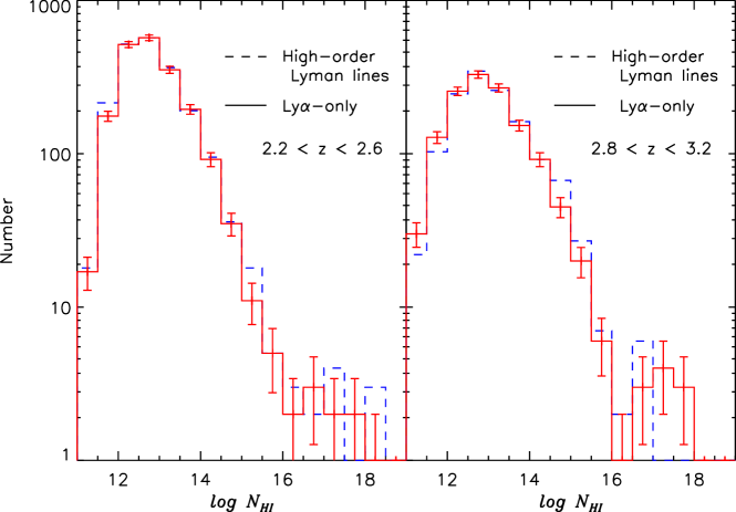
Figure 1: Numbers of absorption lines as a function of $N_{\mathrm{{H\textsc{i}}}}$ at $2.2\!<\!z\!<\!2.6$ and $2.8\!<\!z\!<\!3.2$. The Ly$\alpha$-only fits are shown as solid lines, while the high-order Lyman fits are marked as dashed lines. Solid errors indicate the 1$\sigma$ Poisson errors of the Ly$\alpha$-only fits.

Fig. 1 shows the numbers of absorption lines as a function of $N_{\mathrm{{H\textsc{i}}}}$ for both fitting analyses at the two redshift ranges, $2.2\!<\!z\!<\!2.6$ and $2.8\!<\!z\!<\!3.2$, in order to illustrate the differences at high and low redshifts. The differences between the two samples occurs mostly at $N_{{H\textsc{i}}}\geq 10^{14.5}$ cm^-2 and at $N_{{H\textsc{i}}}\leq 10^{12}$ cm^-2. This difference in the line numbers at $N_{{H\textsc{i}}}\geq 10^{14.5}$ cm^-2 seems to be stronger at $2.8<z<3.2$, although it is still within 2$\sigma$ Poisson errors. The line numbers at $N_{{H\textsc{i}}}\leq 10^{12}$ cm^-2 are more susceptible to the incompleteness which depends on the local S/N than the difference between the two fitting methods. The difference at other column density ranges is smaller, which in turn leads us to expect that there is no significant difference between the Ly$\alpha$-only fit and the high-order Lyman fit.

We restrict our present analysis to $\log N_{{H\textsc{i}}}\!=\![12.75,17]$ at all redshifts. As clearly seen in Fig. 1, the incompleteness becomes quite severe for $\log N_{{H\textsc{i}}}\!\leq\!12.5$ and redshifts $z\!>\!3$ (Kim et al. 1997, 2002). Therefore, the lower $N_{{H\textsc{i}}}$ limit was chosen to be $\log N_{{H\textsc{i}}}\!=\!12.75$. We chose $\log N_{{H\textsc{i}}}\!=\!17$ as the upper $N_{{H\textsc{i}}}$ limit since we wanted to analyze only the Ly$\alpha$ forest whose traditional definition is an absorber with $\log N_{{H\textsc{i}}}\!<\!17.2$ (above which it is referred to as a Lyman limit system (Tytler 1982)). Additionally, absorbers at $\log N_{{H\textsc{i}}}\!>\!17$ are very rare (Fig. 1).

Note that the availability of the high-order Lyman series depends on the redshift of the quasar and whether the sightline contains a Lyman limit system. In addition, the amount of blending affects whether a reliable column density can be measured. At high redshifts $z_{\mathrm{em}}\,>\,3$, line blending becomes severe. However, most UVES spectra also covers down to 3050 Å  where Lyman lines higher than Ly$\delta$ are available. On the other hand, at $z_{\mathrm{em}}<2.5$ the available high-order Lyman lines are rather limited, with mostly Ly$\beta$ and Ly$\gamma$ available. However, line blending is less problematic than at higher redshifts. We have generated tens of saturated artificial absorption lines and fitted them including and excluding high-order Lyman lines. These simulations show that unblended absorption features at $N_{{H\textsc{i}}}\leq 10^{17}$ cm^-2 can be reasonably well constrained with Ly$\alpha$ and Ly$\beta$ only. This indicates that our $N_{{H\textsc{i}}}$ can also be considered reliable even at $z<2.5$ with Ly$\alpha$ and Ly$\beta$ only.

Figure 2: Total absorption distance $X(z)$ covered with our sample of 18 high-redshift quasars. The solid line is for the Ly$\alpha$-only fit, while the dashed one is for the high-order fit.

The absorption distance is obtained by integrating the Friedmann equation for a $\Omega_{m}=0.3$ and $\Omega_{\Lambda}=0.7$ universe, and is given by

$$X(z)=\int\frac{H_{0}}{H(z)}\left(1+z\right)^{2}\mathrm{d}z$$ (1)

(Bahcall & Peebles 1969), where $H_{0}$ is the Hubble constant at $z=0$. The total absorption distance $X(z)$ covered by the spectra for both Ly$\alpha$-only and high-order fits is shown in Fig. 2. The redshift coverage of our sample steadily increases with decreasing redshift until it reaches its maximum at $z\!\sim\!2.1$. For redshifts below $z\!<\!1.9$ the coverage decreases rapidly and our sample ends at $z=1.7$. Note that the lowest redshift possible for the high-order Lyman line analysis is $z\!\sim\!1.97$, while the Ly$\alpha$-only fit analysis is possible down to $z\sim 1.7$. Due to the reduced redshift coverage in the high-order Lyman range of individual sight lines caused by intervening Lyman limit systems, the sample coverage of the high-order fit analyses is reduced between $2.4\!<\!z\!<\!2.7$. At the high redshift end $z\!>3.22$, the number of available forest lines decreases and the sample consists of only one line of sight. The low redshift limit for the high-order fit was set to be the lowest redshift without any saturated lines when no Ly$\beta$ is available for each quasar. This criterion restricts our high-order Lyman fit analysis to $1.9\!<\!z\!<\!3.2$. Since the redshift coverage of low-z quasars for the high-order fit is shorter than the one for the Ly$\alpha$-only fit and the high-$N_{\mathrm{{H\textsc{i}}}}$ forest clusters stronger at lower $z$ (Kim et al. 2002), the quasar-by-quasar $\mathrm{d}n/\mathrm{d}z$ at $z\!\sim\!2$ from the high-order fit analysis is expected to suffer from the low number statistics.

In Table 1, Columns 3–6 summarise the redshift range used for the different analysis. Column 3 lists the redshift range of the Ly$\alpha$ forest region analysed for the number density evolution in the Ly$\alpha$-only fit. For the differential column density evolution of the Ly$\alpha$-only fit, we used the redshift range listed in Column 5. Column 4 and Column 5 list the redshift range for which the high-order Lyman fit can be performed and the one for which the high-order Lyman fit was done, respectively. The region is listed only when it is different from the Ly$\alpha$-only fit region in Column 3. Since there are no strongly saturated Ly$\alpha$ lines at $1.90\!<\!z\!<\!1.98$ for some low-$z$ quasar sightlines, we used a lower redshift range than the one listed in Column 4 for the high-order Lyman fit analysis for these sightlines. Column 6 shows the redshift range excluded for the C iv-enriched H i study in Section 5. Due to the wavelength gaps caused by the UVES dichroic setup, the covered C iv redshift ranges are smaller than the Ly$\alpha$ forest coverage listed in Column 3. The region of $\pm 200$ km s^-1 from the gap was excluded, and only the redshift range covering both C iv doublets was included in the analysis. The blank entries mean that the analyzed $z_{\mathrm{{C\textsc{iv}}}}$ is the same as the forest $z_{\mathrm{Ly,high-order}}$. Q0055$-$269 and J2233$-$606 are excluded in the Ly$\alpha$–C iv forest study due to their lower S/N in the C iv region.

In the HE2347$-$4342 Ly$\alpha$ forest region, there are very strong O vi absorptions mixed with the two saturated Ly$\alpha$ absorption systems at 4012–4052 Å (Fechner et al. 2004). Since the fitted line parameters for these Ly$\alpha$ systems cannot be well constrained (their corresponding Ly$\beta$ is below the partial Lyman limit produced by the $z\!\sim\!2.738$ systems), we excluded this forest region toward HE2347$-$4342. In the J2233$-$606 sightline, there are two partial Lyman limit systems at 3489 Å ($z\!\sim\!1.870$) and 3558 Å ($z\!\sim\!1.926$) and several high column density forest absorbers at 3400–3650Å. To derive a robust $N_{H\textsc{i}}$, we included the HST/STIS echelle spectrum of J2233$-$606 at 2280–3150 Å. The resolution in this wavelength region is $\sim\!10$ km s^-1 and its S/N is $\sim\!8$ per pixel (0.05 Å).

Table 1 also lists the S/N of each quasar spectrum in Column 7. The number outside the bracket is a S/N of the H i forest region. The first number inside the bracket is a typical S/N of the C iv region at $1.9<z<2.4$, while the second is for $2.4<z<3.2$. The dotted entries inside the bracket indicate that no C iv forest region is available for a given redshift range. The low redshift bin of the C iv forest covers the wavelength region where the different CCDs from two dichroic settings were used at $\sim\!4780$ Å(or $z\sim 2.1$). This leads to a much lower S/N at $\leq\!4780$ Å ($z<2.1$). When the lower S/N region is larger than 20% of the whole C iv forest range, two numbers were listed inside the parentheses. The first number corresponds to the lower S/N at $1.9<z<2.1$, while the second number is for the higher S/N at $2.1<z<2.4$.

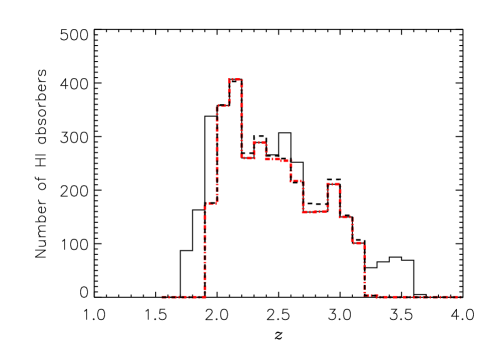
Figure 3: Number of H i absorbers with $\log N_{{H\textsc{i}}}\!=\![12.75,17]$ as function of redshift in our our sample of 18 high-redshift quasars. The solid line is for the Ly$\alpha$-only fit. The dashed line is for the high-order fit, while the red heavy dot-dashed line is for the Ly$\alpha$-only fit for the redshift range used for the high-order fit.

In addition, regions within $\pm 50$ Å to the center of a sub-damped Ly$\alpha$ system ($N_{\mathrm{{H\textsc{i}}}}\geq 10^{19}$ cm^-2) are excluded, since they are associated directly with intervening high-$z$ galactic disks/halos and could have a possible influence on the apparent line densities in the forest. The sightline toward Q0453$-$423 includes a sub-DLA, which introduces a gap in the Ly$\alpha$ redshift range. All the calculations toward Q0453$-$423 account for this redshift gap correctly. However, they are plotted as a single data point and their plotted redshift range is the whole Ly$\alpha$ redshift range without showing a gap. The sightlines toward PKS2126$-$158 and Q0420$-$388 also contain an intervening sub-DLA, which shortens the continuously available redshift coverage for the high-order fit. Column 8 of Table 1 lists the observed wavelength of a Lyman limit (LL, 912 Å in the rest-frame wavelength) of each quasar, which is defined as the wavelength below which the observed flux becomes 0. The values are taken from Kim et al. (2004). When a Lyman limit is not detected within available data, it is denoted to be less than the lowest available wavelength. Column 9 of Table 1 notes information on sub-DLAs along the sightline. When a sub-damped Ly$\alpha$ system exists along the sightline, we discarded 50 Å centred at the sub-DLA each side to exclude its influence on the forest, such as a higher frequency or lack of higher-column density forest. The total number of H i lines for $\log N_{{H\textsc{i}}}\!=\![12.75,17]$ at $1.9<z<3.2$ is 3077 for the high-order Lyman fit sample. The Ly$\alpha$-only fit sample has 3778 H i lines at the total redshift range listed in the 3rd column of Table 1.

In Fig. 3 the number of H i absorbers with $\log N_{\mathrm{{H\textsc{i}}}}=[12.75,17]$ from both fitting methods is shown as a function of redshift. The number of absorbers obtained from each fitting analysis is roughly proportional to the absorption distance coverage. Therefore, our sample shows the highest H i absorber numbers around redshift $z\sim 2$ for each fitting analysis, where the sample absorption distance coverage also reaches its maximum. Sometimes the high-order fit analysis (dashed line) reveals a slightly higher number of absorbers between $2<z<3$. This is because what appear to be single saturated Ly$\alpha$ lines may have more than one component present in the corresponding higher order Lyman lines. At $z\sim 2$, the number of the Ly$\alpha$-only-fit absorbers (heavy dot-dashed line) is slightly larger than the high-order-fit absorbers. This is caused by the fact that some simple saturated lines with $\log N_{\mathrm{{H\textsc{i}}}}\!<\!17$ in the Ly$\alpha$-only fit analysis are actually absorbers with $\log N_{\mathrm{{H\textsc{i}}}}\!>\!17$ in the high-order fit analysis. Since the Ly$\alpha$-only fit gives a lower $N_{\mathrm{{H\textsc{i}}}}$ limit for a saturated line, these lines are included in the Ly$\alpha$-only fit sample, but excluded in the high-order fit sample in Fig. 3.

3 Comparison with previous studies using Ly$\alpha$ only

In Sect. 2 we have shown that including higher order transitions in the fitting process slightly alters the column density statistics at $\log N_{H\textsc{i}}\!>\!15.0$. In order to compare our quasar sample with previous studies based only on the Ly$\alpha$ transition, we briefly present the column density distribution and evolution derived from the Ly$\alpha$-only fit in this section. A large redshift coverage is very important in the study of the absorber number density. Therefore we used all Ly$\alpha$ lines found in the whole available Ly$\alpha$ redshift ranges listed in Column 3 of Table 1 in this section. On the other hand, the differential density distribution function is not sensitive to a large redshift coverage. Thus, only the Ly$\alpha$ lines at $1.9\!<\!z\!<\!3.2$ are analysed for the distribution function study. A detailed analysis using the high-order fit is presented in Section 4. All the results from this section are tabulated in Appendix A.

3.1 Absorber number density evolution $\mathrm{d}n/\mathrm{d}z$

The absorber number density $n(z)$ is measured by counting the number of H i absorption lines for a given column density range for each line of sight. The line count $n$ is then divided by the covered redshift range $\Delta z$ to obtain $\mathrm{d}n/\mathrm{d}z$. If forest absorbers have a constant size and a constant comoving number density, its number density evolution due to the Hubble expansion can be described as

$$\frac{\mathrm{d}n}{\mathrm{d}z}=\pi R^{2}N_{0}cH(z)^{-1}(1+z)^{2},$$ (2)

where $R$ is the size of an absorber, $N_{0}$ is the local comoving number density and $c$ is the speed of light (Bahcall & Peebles 1969). For our assumed cosmology, Eq. 2 becomes

$$\frac{\mathrm{d}n}{dz}\propto\frac{(1+z)^{2}}{\sqrt{0.3(1+z)^{3}+0.7}}.$$ (3)

At $1<z<4.5$, Eq. 3 has an asymptotic behaviour of $\mathrm{d}n/\mathrm{d}z\propto(1+z)^{\sim 0.6}$, while at $z<1$ it becomes $\mathrm{d}n/\mathrm{d}z\propto(1+z)^{\sim 1.15}$. For higher redshifts the asymptotic behaviour becomes $\mathrm{d}n/\mathrm{d}z\propto(1+z)^{0.5}$. Any differences in the observed exponent from what is expected from Eq. 3 indicate that the absorber size or/and the comoving density are not constant.

Empirically, $\mathrm{d}n/\mathrm{d}z$ is described as $\mathrm{d}n/\mathrm{d}z=A(1+z)^{\gamma}$. It has been known that $\mathrm{d}n/\mathrm{d}z$ evolves more rapidly at higher column densities. At $z\!>\!1.5$, a $\gamma\!\sim\!2.9$ is found for $N_{\mathrm{{H\textsc{i}}}}=10^{14-17}$ cm^-2, and $\gamma\!\sim\!1.4$ for $N_{\mathrm{{H\textsc{i}}}}=10^{13.1-14}$ cm^-2 (Kim et al. 2002). At $z\!<\!1.5$, Weymann et al. (1998) found $\gamma\!\sim\!0.16$ and $A\!\sim\!35$ for absorbers with a rest-frame equivalent width greater than 0.24 Å from HST/FOS data. Later studies on $\mathrm{d}n/\mathrm{d}z$ based on the profile fitting or curve of growth analysis using better-quality data from HST/STIS and HST/GHRS show a factor of $\sim$2–3 lower $\mathrm{d}n/\mathrm{d}z$ than the one found by Weymann et al. (1998). These studies also show a larger scatter in $\mathrm{d}n/\mathrm{d}z$ at $z<0.2$ with $A\!\sim\!5$–22 (Lehner et al. 2007; Williger et al. 2010). Part of this scatter is thought to be caused by inhomogeneous data quality, analysis methods, and cosmic variance. Unfortunately high-quality data lack a complete $z$ coverage at $z\!<\!1.5$, missing mostly at $0.4\!<\!z\!<\!1.0$. Keep in mind that the FOS result and most available ground-based results at $z>1.5$ in the literature are based on the Ly$\alpha$ lines only, while most space-based results at $z<1.5$ are using the available high-order Lyman series. Therefore, it is not possible to derive a robust power-law slope $\gamma$ of $\mathrm{d}n/\mathrm{d}z$ at $0\!<\!z\!<\!3.5$. Strictly speaking, a fair comparison should be made on the data with similar qualities and uniform analyses.

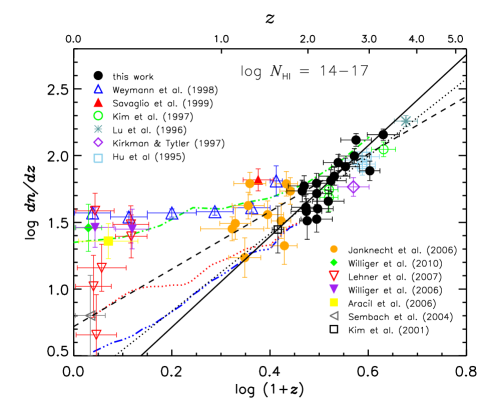
Figure 4: The number density evolution of the Ly$\alpha$ forest in the column density range $\log N_{\mathrm{{H\textsc{i}}}}=[14,17]$ of the Ly$\alpha$-only fits. Black filled circles show results from our data set, which is tabulated in Table 7. Other data points indicate various results obtained from the literature. The vertical error bars give the $1\sigma$ Poisson error, while the x-axis error bars show the redshift range covered by each sightline. The solid line shows the fit to our data only. Dashed line is the result including the literature data for $z>1$ ($\log(1+z)>0.3$). The dotted line gives the fit given in Kim et al. (2002). The green dot-dashed curve shows the predicted $\mathrm{d}n/\mathrm{d}z$ evolution based on a quasar-only UV background by Davé et al. (1999). The red dotted and the blue dot-dot-dot-dashed curves at $z<2$ illustrate the predicted $\mathrm{d}n/\mathrm{d}z$ based on momentum-driven wind and no-wind models with a UV background by quasars and galaxies, respectively (Davé et al. 2010).

The number density evolution is illustrated in Figs. 4, 5 and 6 for two different column density ranges: $\log N_{{H\textsc{i}}}=[14,17]$, and $[13.1,14]$. Data compiled from the literature are indicated in the figures: Hu et al. (1995), Lu et al. (1996), Kim et al. (1997), Kirkman & Tytler (1997), Weymann et al. (1998), Savaglio et al. (1999), Kim et al. (2001), Sembach et al. (2004), Williger et al. (2006), Aracil et al. (2006), Janknecht et al. (2006), Lehner et al. (2007) and Williger et al. (2010). To be consistent with our definition of the proximity effect zone, we applied the same $4\,000$ km s^-1 exclusion within the quasar’s Ly$\alpha$ emission line for all the literature data, whenever the line lists from the literature include all the Ly$\alpha$ lines below the Ly$\alpha$ emission line of the quasar. When the published line lists are only for the shorter wavelength region than the entire, available forest region outside the $4\,000$ km s^-1 proximity zone, such as the ones by Hu et al. (1995), no such an exclusion is required. We used all the reported H i lines in the literature mentioned above, without any pre-selection imposed on $N_{\mathrm{{H\textsc{i}}}}$ or $b$ parameters. The latest study on the low-redshift IGM by Williger et al. (2010) found that the number density from the HST/STIS results is a factor of 2–3 lower than the HST/FOS results by Weymann et al. (1998). They applied the same selection criteria on H i absorbers used by Lehner et al. (2007), i.e. measurement errors less than 40% and $b<40$ km s^-1. As H i absorbers tend to have a larger $b$ parameter at lower redshift (Lehner et al. 2007) and larger measurement errors in general, selecting H i absorbers at $b>40$ km s^-1 has a larger impact on $\mathrm{d}n/\mathrm{d}z$ at lower redshift. In addition, as the HST/FOS results are based on the H i sample without any imposed selection criteria, using the full H i lines provides a more straightforward comparison to the HST/FOS result.

We have performed a linear regression to our data in logarithmic space for the various column density bins, using the maximum likelihood method described in Ripley & Thompson (1987). This method accounts for the uncertainties in the number density and incorporates the weighting using the uncertainties. Errors of the fit parameters were obtained using the maximum likelihood method. Linear regressions were once obtained from our data including the literature data and once without them. Since for redshifts $z\lesssim 1$ (or $\log(1+z)\lesssim 0.3$) the number density evolution could remain constant with redshift, cf. Weymann et al. (1998), only the literature data with redshift $z\!>\!1$ was used for the fit. The resulting parameters are given in Tables 2.

Fig. 4 shows the $\mathrm{d}n/\mathrm{d}z$ evolution for the column density interval of $\log N_{{H\textsc{i}}}=[14,17]$. Our results (filled circles) agree well with previous findings at $z>1.5$ ($\log(1+z)>0.4$), confirming that there is a real sightline variation in $\mathrm{d}n/\mathrm{d}z$. Kim et al. (2002) notes that the scatter between different sightlines increases as $z$ decreases down to $z\!\sim\!2$. In fact, the data of Janknecht et al. (2006) at redshifts below $z\!\sim\!2$ ($\log(1+z)\sim 0.45$) indicate that the scatter might well increase at lower $z$, although the errors are still very large to draw any firm conclusions. Considering that the FOS result is based on the equivalent width measurement, and the conversion from the equivalent width to the column density requires the $b$ parameters of individual absorbers, which are ill-constrained at the FOS resolution, the full HST/STIS H i sample toward some sightlines is in good agreement with the HST/FOS result (blue open triangles), although there still is a large sightline variation. The full H i sample at $z<0.4$ strongly supports the previous conclusion obtained by the HST/FOS result, that $\mathrm{d}n/\mathrm{d}z$ flattens out at $z\leq 1.5$.

Table 2: Linear regression results for $\mathrm{d}n/\mathrm{d}z$

a) Using the Ly$\alpha$-only fits and fits including literature data for $z\!>\!1$
	UVES quasar by quasar		quasar by quasar with lit.
$\Delta\log N_{H\textsc{i}}$	$\log A$	$\gamma$	$\log A$	$\gamma$
$13.64-17.0$	$0.78\pm 0.14$	$2.55\pm 0.27$	$1.13\pm 0.06$	$1.90\pm 0.11$
$14.0-17.0$	$0.03\pm 0.20$	$3.40\pm 0.36$	$0.72\pm 0.08$	$2.16\pm 0.14$
$14.5-17.0$	$-0.14\pm 0.26$	$3.02\pm 0.48$	$0.46\pm 0.11$	$1.94\pm 0.20$
$13.1-14.0$	$1.46\pm 0.11$	$1.67\pm 0.21$	$1.52\pm 0.05$	$1.51\pm 0.09$
$12.75-14.0$	$1.98\pm 0.08$	$1.13\pm 0.16$
b) The mean $\mathrm{d}n/\mathrm{d}z$ using the Ly$\alpha$-only fits at $0<z<4$
$\Delta\log N_{H\textsc{i}}$	$\log A$	$\gamma$
$13.1-14.0$	$1.88\pm 0.03$	$0.89\pm 0.06$
$14.0-17.0$	$1.03\pm 0.07$	$1.61\pm 0.12$
c) The UVES high-order fits at $1.9<z<3.2$
	quasar by quasar		Mean sample
$\Delta\log N_{H\textsc{i}}$	$\log A$	$\gamma$	$\log A$	$\gamma$
$12.75-14.0$	$1.85\pm 0.12$	$1.38\pm 0.22$	$1.89\pm 0.13$	$1.28\pm 0.24$
$14.0-17.0$	$-0.76\pm 0.29$	$4.91\pm 0.53$	$-0.65\pm 0.36$	$4.65\pm 0.66$

The linear regression to our results only (the solid line) with $\gamma=3.40\pm 0.36$ is different at 3$\sigma$ from the fit to all the available data at $z>1$ ($\log(1+z)>0.3$) which yields $\gamma=2.16\pm 0.14$ (the dashed line). This discrepancy is mainly due to the sparse data of our sample at higher redshift $z>3.5$ ($\log(1+z)>0.65$) and the missing constraints at $z<2.0$. The discrepancy is also in part caused by how the power-law fit is performed. Our maximum likelihood fit does the weighted fit. This gives a higher weight on higher-$z$ data points where the 1$\sigma$ Poisson error is usually smaller. The non-weighted fit for our UVES data only results in a steeper power-law slope, $(-0.84\pm 0.24)\times(1+z)^{5.02\pm 0.76}$. The non-weighted fit for all the data at $z>1$ is $(0.76\pm 0.18)\times(1+z)^{2.00\pm 0.25}$.

Interestingly, some earlier numerical simulations and theories with a quasar-only UV background have shown that there should be a break in the $\mathrm{d}n/\mathrm{d}z$ evolution at $z\!\sim\!2$ due to the decrease in the quasar number density, thus less available H i ionising photons (Theuns et al. 1998; Davé et al. 1999; Bianchi et al. 2001). The green dot-dashed curve in Fig. 4 shows one of such predicted $\mathrm{d}n/\mathrm{d}z$ evolutions by Davé et al. (1999), which outlines the Weymann et al. $\mathrm{d}n/\mathrm{d}z$ reasonably well. However, more recent simulations by Davé et al. (2010) predict different $\mathrm{d}n/\mathrm{d}z$ evolutions. These simulations are based on the various galactic wind models and the UV background contributed both by quasars and galaxies. The red dotted and the blue dot-dot-dot-dashed curves at $z<2$ illustrate their predicted $\mathrm{d}n/\mathrm{d}z$ based on momentum-driven wind and no-wind models, respectively. These newer simulations predict that $\mathrm{d}n/\mathrm{d}z$ continuously decreases with decreasing redshift. Their momentum-driven wind model agrees reasonably well with the observations by HST/STIS with the H i absorber selection imposed (measurement errors less than 40% and $b<40$ km s^-1), but not with the Weymann et al. data. A better, uniform dataset from HST/COS observations should resolve this discrepancy at $z<0.5$.

For the column density interval for stronger absorbers $\log N_{\mathrm{{H\textsc{i}}}}=[14.5,17.0]$, our data shows that the evolution continues to follow the empirical power-law with $\gamma=3.02\pm 0.48$ (see Table 2). However, the scatter between different sightlines is large as stronger absorbers are rare at all redshifts (Davé et al. 2010). There are more than 3$\sigma$ difference between the lowest $\mathrm{d}n/\mathrm{d}z$ sightline and the highest $\mathrm{d}n/\mathrm{d}z$ sightline at $z\!\sim\!2$. Kim et al. (2002) discuss the possibility on whether the column density evolution flattens out at $z\!<\!2.5$ ($\log(1+z)\!<\!0.55$) for this column density interval. Even though more data points are available in this study, this question cannot be conclusively answered and more data covering lower redshifts are required.

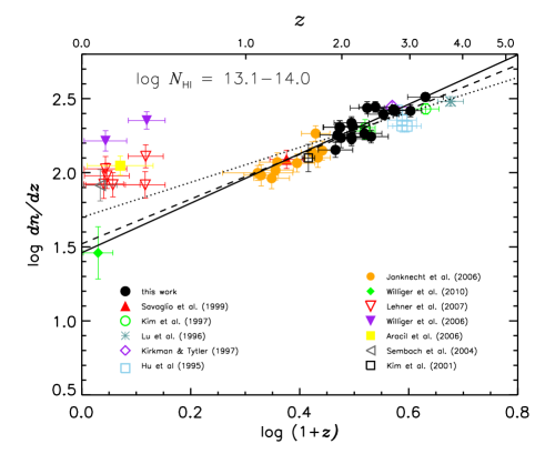
Figure 5: The number density evolution of the Ly$\alpha$ forest in the column density range $\log N_{\mathrm{{H\textsc{i}}}}=[13.1,14.0]$. All the symbols have the same meaning as in Fig. 4.

The line number density evolution for low column density systems in the range of $\log N_{\mathrm{{H\textsc{i}}}}=[13.1,14.0]$ is presented in Fig. 5. Similar to Fig. 4, it suggests that the flattening of $\mathrm{d}n/\mathrm{d}z$ at $z<1.5$ might continue at the lower column density range. However, the sightline variation at $z<0.4$ is larger at this column density range. This is in part caused by different analysis methods and different S/N STIS data used by different studies. For example, the number density measured in the STIS spectrum toward PKS0405$-$123 is different between the Williger et al. (2006) work (filled purple upside-down triangles) and the Lehner et al. (2007) work (two of open red upside-down triangles). Again the results from our data agree well with previous results found in the literature at $z\!>\!1.5$. The linear regression to our data at $z\!>1.5$ gives $\gamma\approx 1.67$, comparable to the fit including all available literature data points at $z\!>\!1.0$. However, these results do not compare well with the linear regression obtained by Kim et al. (2002) with $\gamma=1.18\pm 0.14$ (the dotted line), a shallower $\mathrm{d}n/\mathrm{d}z$ evolution. This discrepancy arises due to their rather small sample size at $z\!<\!2.5$ and more severe line blending at higher redshifts. Given a larger cosmic variance at lower redshifts, the sample size becomes more important. At the same time, line blending at high redshifts makes the detection of weak absorbers difficult. This incompleteness effect has been shown to underestimate the line number density of low column density systems at $\log N_{\mathrm{{H\textsc{i}}}}=[13.3,13.6]$ by $\sim\!17\%$ at $z\!\sim\!3$ ($\log(1+z)\!\sim\!0.6$) and by $\sim\!35\%$ at $z\!\sim\!4$ (Giallongo et al. 1996). Both effects tend to flatten the evolution observationally from its true value. In addition, the robust estimate of the exponent $\gamma$ requires a large $z$ leverage.

Figure 6: The mean number density evolution of the Ly$\alpha$ forest. The vertical error bars give the $1\sigma$ Poisson error, while the x-axis error bars show the redshift range covered by each data point. The data point with the dotted error bar indicate the Janknecht et al. (2006) data. The dashed straight lines mark the fit to the mean data excluding the Janknecht et al. (2006) data.

Even though there are not many sightlines covering $0.5\!<\!z\!<\!1.5$, we calculated the mean $\mathrm{d}n/\mathrm{d}z$ from all the combined H i fitted line lists including the literature data in Fig. 6. This mean $\mathrm{d}n/\mathrm{d}z$ is not an averaged value of the individual sightlines. The literature data used in the combined line list include all the quasar sightlines shown in Figs. 4 and 5, except the HST/FOS Weymann et al. (1998) data, the Williger et al. (2006) data and the Savaglio et al. (1999) data. The HST/FOS data was excluded since they were based on the equivalent width measurements, while the Williger et al. (2006) data suffered from noise features. The Savaglio et al. (1999) result is from a single sightline and provides the only data point besides the Janknecht et al. (2006) data at $z\sim 1$. Although the Janknecht et al. (2006) data also suffer from noise, they were from 9 sightlines. We opted to use a result based on the analysis of multiple sightlines from a single study. This helps to reduce any systematics caused by combining results from different studies at $z\sim 1$. For $z<0.4$, the systematic uncertainty is larger since the line lists used are produced by different studies.

At $\log N_{\mathrm{{H\textsc{i}}}}\!=\![13.1,14.0]$, there might occur a flattening at $z\!\sim\!1$, if the Janknecht data were included. At $\log N_{\mathrm{{H\textsc{i}}}}\!=\![14,17]$, a single power law with $\gamma=1.61\pm 0.12$ does not give a good fit at $0\!<\!z\!<\!4$, regardless of the inclusion of the Janknecht et al. data. It remains to be seen whether a single power law fits the $\mathrm{d}n/\mathrm{d}z$ evolution for both high and low column density ranges at $z=0.4$. It should be noted that the $\mathrm{d}n/\mathrm{d}z$ of Lyman limit systems with a column density of $\log N_{{H\textsc{i}}}=[17.2,19.0]$ does not fit to a single power law. It shows a slower evolution at $z<2$ and evolves rapidly at $z>2$ (Prochaska et al. 2010), while the $\mathrm{d}n/\mathrm{d}z$ of damped Ly$\alpha$ systems with $\log N_{{H\textsc{i}}}=[20.3,22.0]$ shows a single power-law evolution with a slope $\gamma=1.27\pm 0.11$ at $0<z<4.5$ (Rao et al. 2006) .

Our results indicate that higher column density forest systems evolve more rapidly than low column density systems and the number density of high column density systems decreases faster with decreasing redshift. The increase in the scatter at redshifts $z\!<\!2.5$ might indicate the transition point where the evolving number density changes into a non-evolving one, as is predicted in earlier numerical simulations by Theuns et al. (1998) and Davé et al. (1999).

3.2 The differential column density distribution function

The differential column density distribution function (CDDF) is defined as the number of absorbers per unit absorption distance $X(z)$ and per unit column density $N_{H\textsc{i}}$. The absorption distance is calculated using Eq. 1. Empirically, the differential distribution function is reasonably well described by a single power law at $z\sim 3$ at $\log N_{{H\textsc{i}}}=[13,22]$ as

$$\frac{\mathrm{d}n}{\mathrm{d}N_{H\textsc{i}}\,\mathrm{d}X}=\left(\frac{\mathrm{d}n}{\mathrm{d}N_{H\textsc{i}}\,\mathrm{d}X}\right)_{0}N_{H\textsc{i}}^{\beta},$$ (4)

where $\left(\mathrm{d}n/(\mathrm{d}N_{H\textsc{i}}\,\mathrm{d}X)\right)_{0}$ gives the normalisation point of the distribution function and $\beta$ denotes its slope. However, the detailed shape of the differential column density distribution function is dependent on the $N_{{H\textsc{i}}}$ column density range (Prochaska et al. 2010; Altay et al. 2011). It shows a flattening around the transition from the forest to the Lyman limit systems at $N_{H\textsc{i}}$ at $\log N_{H\textsc{i}}\!\sim\!17$. Then it shows a steepening at $\log N_{H\textsc{i}}\!\sim\!20$ where a transition occurs from the sub-damped Ly$\alpha$ systems to the damped Ly$\alpha$ systems.

Figure 7: The differential column density distribution at $1.9<z<3.2$ using the Ly$\alpha$-only fits. Both black ($\log N_{H\textsc{i}}\!\geq\!12.75$) and grey ($\log N_{H\textsc{i}}\!<\!12.75$) data points show the results from our quasar sample. The grey data points mark the column densities that are affected by incompleteness. The stars are the data points obtained by Petitjean et al. (1993). The filled circles at $\log N_{H\textsc{i}}\!>\!20.1$ and at $19\!<\!\log N_{H\textsc{i}}\!<\!20.1$ are from the SDSS II DR7 at $<z>\,=3.02$ by Noterdaeme et al. (2009) and from O’Meara et al. (2007) at $<z>\,=3.1$, respectively. The solid line gives the power law fit to our data for $\log N_{H\textsc{i}}\!=\![12.75,14]$. The dotted line represent the fit obtained by Hu et al. (1995), while the dashed line represents a theoretical prediction at $z\sim 3$ by Altay et al. (2011). The vertical error bars indicate $1\sigma$ Poisson errors, while the x-axis error bars show the $N_{\mathrm{{H\textsc{i}}}}$ range covered by each data point. Gas overdensities on the top x-axis are computed using Eq. 10 from Schaye (2001) at $z\!=\!2.55$ (see text for details).

In Fig. 7 we present the results using the Ly$\alpha$-only fits at $1.9<z<3.2$. Note that the redshift range used for the CDDF analysis is different from the one used for the $dn/dz$ analysis in Section 3.1. The total absorption distance $X(z)$ at $1.9\!<\!z\!<\!3.2$ is 21.8165. The binsize of $\log N_{\mathrm{{H\textsc{i}}}}\!=\!0.25$ is used at $\log N_{\mathrm{{H\textsc{i}}}}\!=[12.0,15.0]$, then the binsize of 0.5 at $\log N_{\mathrm{{H\textsc{i}}}}\!=[15.0,18.0]$. To increase the column density coverage, we include results from Noterdaeme et al. (2009) and O’Meara et al. (2007) for $\log N_{\mathrm{{H\textsc{i}}}}>19$ at $z\sim 3$ from the SDSS II DR7 data. The top x-axis is in units of the gas overdensity $\delta$ which was computed according to Eq. 10 by Schaye (2001)

$$N_{H\textsc{i}} \sim 2.7\times 10^{13}\,\left(1+\delta\right)^{3/2}\,\times$$ (5)

$$\times\,T_{4}^{-0.26}\,\Gamma_{12}^{-1}\left(\frac{1+z}{4}\right)^{9/2}\left(\frac{\Omega_{b}h^{2}}{0.02}\right)^{3/2}\left(\frac{f_{g}}{0.16}\right)^{1/2}\textrm{ cm}^{-2}.$$

Here, the gas temperature $T$ is assumed to be $T=T_{4}\times 10^{4}\textrm{ K}$, the photoionisation rate $\Gamma=\Gamma_{12}\times 10^{-12}\textrm{ sec}^{-1}$. The parameter $f_{g}$ denotes the fraction of mass in gas. The IGM gas temperature is assumed to be governed by the effective equation of state $T=T_{0}(1+\delta)^{\gamma-1}$, where $T_{0}$ is the temperature at the cosmic density (Hui & Gnedin 1997). For $\Gamma_{12}$ and $\gamma$, we interpolated results obtained by Bolton et al. (2008). We assumed that $T_{0}$ is $2\times 10^{4}\textrm{ K}$, $f_{g}=0.16$, and $\Omega_{b}h^{2}=0.0227$ (Schaye 2001). As the same overdensity corresponds to a different $N_{H\textsc{i}}$ at different $z$, the overdensity plotted in Fig. 7 is at the mean redshift, $z\!=\!2.55$.

We compare our results with the observations by Petitjean et al. (1993) and Hu et al. (1995). Our results are in good agreement with the Petitjean et al. (1993) data over the whole column density range down to $\log N_{H\textsc{i}}\sim 13.5$, following a power law at $\log N_{H\textsc{i}}=[12.75,14]$. At smaller column densities $\log N_{H\textsc{i}}<12.75$, the CDDF starts to deviate from a power law due to the sample incompleteness for weak absorbers (Kim et al. 1997). From the linear regression, we find $\log\left(\mathrm{d}n/(\mathrm{d}N_{{H\textsc{i}}}\,\mathrm{d}X)\right)_{0}=7.34\pm 0.42$ and a slope of $\beta=-1.43\pm 0.03$ for the $\log N_{H\textsc{i}}=[12.75,14]$ range (the solid line). This result is slightly lower than $\beta=-1.46$ (no errors given) by Hu et al. (1995) (the dotted line) or $\beta=-1.49\pm 0.02$ by Petitjean et al. (1993).

The distribution function becomes steeper at $\log N_{{H\textsc{i}}}\!>\!15$, then becomes shallower at higher $\log N_{{H\textsc{i}}}$, as previously observed (Petitjean et al. 1993; Kim et al. 1997; Prochaska et al. 2010). This result agrees well with the theoretical prediction at $z\sim 3$ (the dashed line) by Altay et al. (2011) at $\log N_{H\textsc{i}}\leq 16$, but starts to show a noticeable disagreement at the 1–3$\sigma$ level at $\log N_{H\textsc{i}}=[16,18]$, in part due to the lack of enough high-column density systems in our small sample. We will address the shape of the CDDF in more detail in the next section using results from the high-order fit sample.

4 Analysis using higher-order Lyman lines

In the last section, we checked the Ly$\alpha$ absorber number density evolution and the differential column density distribution obtained from the Ly$\alpha$-only fits for consistency with previous studies. The analysis is now revisited with the results from the Voigt profile analysis including the higher order transitions at $1.9\!<\!z\!<\!3.2$, hence a sample with a more reliable $N_{\mathrm{{H\textsc{i}}}}$. Therefore, it can be established whether the dip seen in the differential column density distribution at $\log N_{\mathrm{{H\textsc{i}}}}$ between $14.5$ and $18$ is a physical feature or just an imprint of uncertainties in $N_{H\textsc{i}}$. All the results from this section are tabulated in Appendix A.

4.1 The mean number density evolution

We now revisit the line number density evolution using the high-order Lyman sample, as described in the previous section. On a quasar by quasar analysis we determine $\mathrm{d}n/\mathrm{d}z$ for a low column density range of $\log N_{H\textsc{i}}=[12.75,14.0]$ and for high column densities of $\log N_{H\textsc{i}}=[14,17]$. The lower column density range is chosen in such a way that the part of the differential column density distribution function which follows a power-law is covered, whereas the $\log N_{H\textsc{i}}=[14,17]$ interval covers those systems responsible for the dip in the column density distribution function.

The results are presented in Fig. 8. Linear regressions from the data are obtained and the resulting parameters are summarised in Table 2. Similar to the previous analysis, the line number density shows a decrease with decreasing redshift. No significant differences between the two different fits are present, even though the total redshift coverage used for the high-order fit is about 20% smaller. In the case of the $\log N_{H\textsc{i}}=[14,17]$ interval, the slope of the power law steepens from the Ly$\alpha$-only slope of $\gamma=3.40\pm 0.36$ to $\gamma=4.91\pm 0.53$ for the high-order fit. This is in part caused by that the number of high column density absorbers is larger in the high-order fit sample. However, the slopes of the two samples are still in the $2\sigma$ uncertainty range, rendering the two results consistent to each other. Similar results are obtained for the $\log N_{H\textsc{i}}=[12.75,14.0]$ range. The slope for the high-order fit increases from $\gamma=1.13\pm 0.16$ for the Ly$\alpha$-only fit to $\gamma=1.38\pm 0.22$. Again, the results from the two samples agree within the $1\sigma$ uncertainty range.

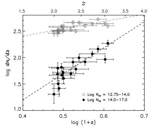
Figure 8: The line number density evolution derived on a quasar by quasar analysis using the high-order Lyman sample for column density intervals of $\log N_{H\textsc{i}}=[12.75,14.0]$ and $\log N_{H\textsc{i}}=[14,17]$. The vertical error bars indicate $1\sigma$ Poisson errors, while the x-axis error bars show the redshift range covered by each sightline. The straight lines denote results from a linear regression to the data with parameters given in Table 2. The data are tabulated in Table 7.

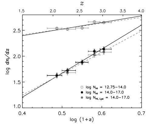
Figure 9: The mean line number density evolution of the combined sample as a function of redshift using the high-order Lyman-series sample for column density intervals of $\log N_{H\textsc{i}}=[12.75,14.0]$ and $\log N_{H\textsc{i}}=[14,17]$. The sample is binned in redshift with $\Delta z=0.26$, starting from $z=1.90$. The vertical error bars indicate $1\sigma$ Poisson errors, while the x-axis error bars show the redshift range covered by each data point. For comparison, the results of the Ly$\alpha$-only fits (grey open circles) are shown for the $\log N_{H\textsc{i}}=[14,17]$ interval. The straight solid lines denote results from a linear regression to the binned data. Two dashed lines represent the mean number density evolution of the Ly$\alpha$-only fit sample for $\log N_{H\textsc{i}}=[14,17]$ ($\log\mathrm{d}n/\mathrm{d}z=(-0.41\pm 0.35)+(4.14\pm 0.63)\times\log(1+z)$) and for $\log N_{H\textsc{i}}=[12.75,14]$ ($\log\mathrm{d}n/\mathrm{d}z=(1.96\pm 0.13)+(1.12\pm 0.24)\times\log(1+z)$), respectively. Exactly same redshift range was used for both fit samples. The data are tabulated in Table 8. The parameters of the fits are given in Table 2.

In previous studies the number density evolution has been usually derived on a quasar by quasar analysis. Previous studies did not have enough quasar sight lines available to sample the number density evolution at smaller redshift interval $\Delta z$, without suffering from small number statistics. Our sample of 18 high-redshift quasars is characterised by a large redshift distance coverage in the redshift range of $1.9<z<3.2$ (see Fig. 2). As a result, a large number of absorption lines is available for small redshift intervals to combine the individual quasar line lists into one big sample. However, due to the larger cosmic variance at low redshifts from the structure formation, the redshift bin size should not be too small. From this combined sample, the evolution of the mean number density is derived in redshift bins of $\Delta z=0.26$, starting from $z=1.90$.

Results of the combined line number density evolution are shown in Fig. 9 for identical column density ranges as used in the quasar by quasar analysis. Error bars have been determined using the bootstrap technique. For comparison, results using the Ly$\alpha$-only fits are overplotted as grey open circles for the high column density bin.

The high column density results are similar to the ones obtained from the Ly$\alpha$-only fits. The number density itself is higher in the high-order fits, since some strongly saturated systems break up into multiple, strong components in the high-order Lyman transition. In addition, three absorbers (two toward HE0940$-$1050 and one toward Q0420$-$388) were found to be a Lyman limit system with $\log N_{H\textsc{i}}\!>\!17$ in the Ly$\alpha$-only fit. Therefore, these systems were not included in the Ly$\alpha$-only results. However, these Lyman limit systems break up into multiple weaker components in the high-order fit and contribute to the number count in the high order fit analysis. However, the differences between the two samples are smaller than the statistical uncertainties.

At low column densities, no noticeable differences between the two samples are observed, as expected.

Again, linear regressions have been determined and their parameters are given in Table 2. At $\log N_{\mathrm{{H\textsc{i}}}}=[12.75,14.0]$, the slope of our combined sample is $\gamma=1.28\pm 0.24$, similar to $\gamma=1.38\pm 0.22$ from the quasar by quasar analysis. At $\log N_{H\textsc{i}}=[14,17]$, the slope of the combined sample $\gamma=4.65\pm 0.66$ is also similar to $\gamma=4.91\pm 0.53$ obtained from the quasar by quasar analysis. The slopes from both analyses of our high-order fit sample at $\log N_{H\textsc{i}}=[14,17]$ are steeper than the ones obtained from the Ly$\alpha$-only fit sample. In particular, the ones from the combined sample differ more than 3$\sigma$. This difference is mainly caused by that the redshift range used for the combined sample is different for two analyses. For the Ly$\alpha$-only fit, the mean $\mathrm{d}n/\mathrm{d}z$ is derived for $0<z<4$, while for the high-order fit it is restricted to $1.9<z<3.2$.

Figure 10: The differential column density distribution at $1.9<z<3.2$ of our quasar sample using the high-order Lyman fit. Black and grey data points show the results from our quasar sample. The grey data points below $\log N_{H\textsc{i}}<12.75$ mark the column densities that are affected by incompleteness. The grey data points above $\log N_{H\textsc{i}}\!>\!12.75$ represent the results from the Ly$\alpha$-only fit. The dashed line represents a theoretical prediction at $z\!\sim\!3$ by Altay et al. (2011). The vertical error bars indicate $1\sigma$ Poisson errors, while the x-axis error bars show the $N_{\mathrm{{H\textsc{i}}}}$ range covered by each data point. The filled circles at $\log N_{\mathrm{{H\textsc{i}}}}\!>\!20.1$ and at $19.0\!<\!\log N_{\mathrm{{H\textsc{i}}}}\!<\!20.1$ are from the SDSS II DR7 at $<\!z\!>\,=3.02$ by Noterdaeme et al. (2009) and from O’Meara et al. (2007) at $<\!z\!>\,=3.1$, respectively. The solid line gives the power law fit to our data for $\log N_{\mathrm{{H\textsc{i}}}}=[12.75,14.0]$. The overdensity plotted on the top x-axis is calculated at $z=2.55$.

4.2 The differential column density distribution function

Using the high-order fits, we have derived the differential column density distribution function (CDDF) for $1.9\!<\!z\!<\!3.2$, analogous to Section 3.2. In Fig. 10 we show the results for the entire redshift range. As in Fig. 7, the binsize of $\log N_{\mathrm{{H\textsc{i}}}}\!=\!0.25$ is used at $\log N_{\mathrm{{H\textsc{i}}}}\!=[12.0,15.0]$, then the binsize of 0.5 at $\log N_{\mathrm{{H\textsc{i}}}}\!=[15.0,18.0]$. The total absorption distance is $X(z)=21.8165$, the same value used for the Ly$\alpha$-only fit CDDF analysis. As with the Ly$\alpha$-only fits, we included observations by Noterdaeme et al. (2009) and O’Meara et al. (2007).

The high-order fit results show a power law relation which is almost identical to the results of the Ly$\alpha$-only fits. As with the Ly$\alpha$-only fits, the differential column density distribution function shows a deviation from the empirical power law at column densities between $14\!<\!\log N_{H\textsc{i}}\!<\!19$. Since the column density distribution deviates from a single power law at $\log N_{H\textsc{i}}\!\sim\!14$, we have individually fitted power laws to four column density intervals of $\log N_{H\textsc{i}}=[12.75,14.0]$, $[14,15]$, $[15,18]$, and $[12.75,18.0]$ at $1.9<z<3.2$, characterising the shape of the distribution function. The resulting parameters are listed in Table 3.

At $\log N_{H\textsc{i}}=[12.75,14.0]$, the linear regression yields a normalisation point of $\log\left(\mathrm{d}N/(\mathrm{d}N_{H\textsc{i}}\,\mathrm{d}X)\right)_{0}=7.41\pm 0.42$ and a slope of $\beta=-1.44\pm 0.03$. This result is almost identical to the Ly$\alpha$-only fit, since differences between the Ly$\alpha$-only and the high-order fits start to be significant at $\log N_{H\textsc{i}}\!>\!15$ (see Fig. 10). The high-order fits show a larger number of absorbers at $15\!<\!\log N_{H\textsc{i}}\!<\!17$ than the Ly$\alpha$-only fits. However, at higher column densities, the number of absorbers is lower for the high-order fits than for the Ly$\alpha$-only fits. This again indicates the breaking up of high column density systems into multiple lower-$N_{H\textsc{i}}$ ones when including higher transitions than Ly$\alpha$. For the entire redshift sample, the slope becomes steeper from $\sim\!-1.44$ to $\sim\!-1.67$ at $\log N_{H\textsc{i}}=[14,15]$. Then at the higher column density range $\log N_{H\textsc{i}}=[15,18]$, the slope becomes shallower to $\sim\!-1.55$, a trend shown in the numerical simulation (the dashed line) by Altay et al. (2011) in Fig. 10.

Table 3: Linear regression results for the differential column density distribution as a function of redshift and column density using the high-order fit. Here the normalisation point $\log\left(\mathrm{d}n/(\mathrm{d}N_{H\textsc{i}}\,\mathrm{d}X)\right)_{0}$ is denoted by $B$.

	$\log N_{H\textsc{i}}=12.75-14.0$		$\log N_{H\textsc{i}}=14.0-15.0$		$\log N_{H\textsc{i}}=15.0-18.0$		$\log N_{H\textsc{i}}=12.75-18.0$
$z$	$B$	$\beta$	$B$	$\beta$	$B$	$\beta$	$B$	$\beta$
$1.9-3.2$	$7.41\pm 0.42$	$-1.44\pm 0.03$	$10.63\pm 1.32$	$-1.67\pm 0.09$	$8.70\pm 1.33$	$-1.55\pm 0.08$	$9.57\pm 0.20$	$-1.60\pm 0.01$
$1.9-2.4$	$8.08\pm 0.55$	$-1.49\pm 0.04$	$11.16\pm 2.07$	$-1.72\pm 0.14$	$7.39\pm 3.00$	$-1.48\pm 0.19$	$10.32\pm 0.31$	$-1.66\pm 0.02$
$2.4-3.2$	$6.72\pm 0.55$	$-1.38\pm 0.04$	$9.96\pm 1.70$	$-1.62\pm 0.12$	$8.64\pm 1.59$	$-1.54\pm 0.10$	$8.59\pm 0.25$	$-1.52\pm 0.02$

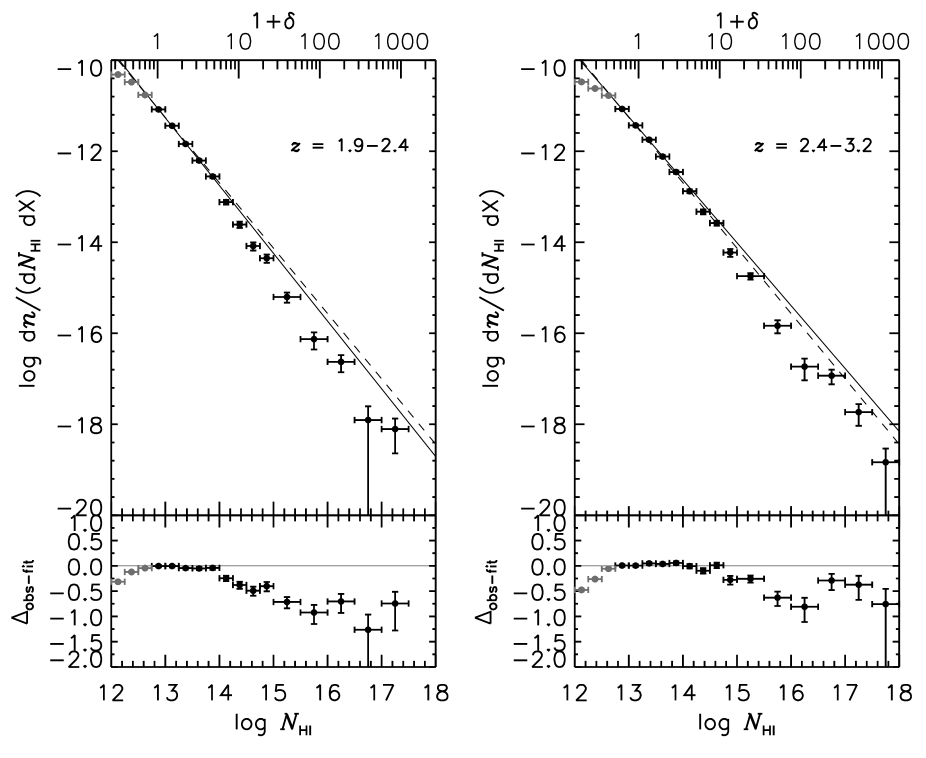
Figure 11: Upper panels: The differential column density distribution as a function of redshift. Both black and grey data points show the results from the high-order Lyman sample. The grey data points at $\log N_{\mathrm{{H\textsc{i}}}}\!<\!12.75$ mark the column densities that are affected by incompleteness. The vertical error bars indicate $1\sigma$ Poisson errors, while the x-axis error bars show the $N_{\mathrm{{H\textsc{i}}}}$ range covered by each data point. The black solid line gives the power law fit for $\log N_{H\textsc{i}}=[12.75,14.0]$ at each redshift bin, whereas the dashed line is the fit to the $z=[1.9,3.2]$ redshift range (see Fig. 10). The overdensity plotted on the top x-axis is calculated at the mean $z$ for each redshift bin. Lower panels: the residuals from the power law fit from the entire redshift range at $\log N_{H\textsc{i}}=[12.75,14.0]$.

In order to determine the redshift evolution of the differential column density distribution, we split the sample into two redshift bins: $z=[1.9,2.4]$ and $[2.4,3.2]$. Fig. 11 shows the CDDF at two different redshift bins, where we overplot the power-law fit at $\log N_{H\textsc{i}}=[12.75,14.0]$ for each redshift bin as the solid line. We also overplot the results of the power-law fit to the entire redshift range $1.9\!<\!z\!<\!3.2$ at the same column density range as the dashed line. For the redshift intervals of $z=[1.9,2.4]$ and [2.4, 3.2], the absorption distance is $X(z)=$ 11.8049 and 10.0116, respectively.

Unfortunately, the uncertainties in the power-law fit parameters at each redshift bin do not allow us to constrain the shape of the distribution as a function of redshift reliably. Comparing the slope of the linear relations shows that the CDDF becomes slightly steeper at low redshift for $\log N_{\mathrm{{H\textsc{i}}}}=[12.75,14.0]$, from $\gamma=-1.38\pm 0.04$ at high $z$ to $\gamma=-1.49\pm 0.04$ at low $z$. However, the slopes are still consistent within 2$\sigma$, i.e. no significant CDDF evolution, cf. Williger et al. (2010). They are also consistent with the result from the entire redshift range within $1\sigma$.

Let us now focus on column densities above $\log N_{\mathrm{{H\textsc{i}}}}\!>\!14.0$. From Fig. 10 we have seen that the differential column density distribution deviates from the power law form for column densities $\log N_{\mathrm{{H\textsc{i}}}}\!>\!14.0$. The lower panels of Fig. 11 show the difference between the observed CDDF and the power-law fit to the CDDF for the entire redshift range (the dashed lines). The entire redshift fit was used since the comparison requires an absolute reference. From the lower panels, it is clear that the deviation from the power law is stronger for the low redshift bin. At the same time, the deviation column density above which the deviation starts to be noticeable is lower at low redshift, from $\log N_{\mathrm{{H\textsc{i}}}}\!\sim\!14.7$ at $2.4\!<\!z\!<\!3.2$ to $\log N_{\mathrm{{H\textsc{i}}}}\!\sim\!14.0$ at $1.9\!<\!z\!<\!2.4$.

Note that no such break in the CDDF has been seen in the $\log N_{\mathrm{{H\textsc{i}}}}=[12.5,16]$ at $z<2$, cf. Fig. 5 of Williger et al. (2010) at $z\!\sim\!0.08$ and Fig. 9 of Ribaudo et al. (2011) at $z\!<\!2$. Both works also found a steeper CDDF slope of $\sim$1.75. Some of the discrepancy is caused by the different fitting methods, the H i selection criterion discussed in Section 3.1 and the column density range over which the power law was performed. On the other hand, Prochaska et al. (2010) found a more significant dip in the column density distribution function at $\log N_{\mathrm{{H\textsc{I}}}}=[14,19]$ at $z\sim 3.7$ (similar to the Altay simulation at $z\!\sim\!3$ indicated by the dashed curve in Figs. 7 and 10). However, the dip shown at $z\!\sim\!3$ in Fig. 11 (the high redshift bin) is not as strong as the one predicted by the Altay simulation, although both results are still considered to be consistent within 2$\sigma$. These differences could be simply due to our small sample size, or due to the different analysis method or due to the strong CDDF evolution between $z\!\sim\!4$ and $z\!\sim\!0$.

Note that the dip shown in Fig. 11 is not caused by self-shielding. Self-shielding causes the number density of absorbers to increase. Self-shielding becomes important at $\log N_{\mathrm{{H\textsc{i}}}}\geq 16$ and its effect becomes evident at $\log N_{\mathrm{{H\textsc{i}}}}\!\geq\!17$ with a shallower slope than the extrapolated one at the lower $\log N_{\mathrm{{H\textsc{i}}}}$ (Altay et al. 2011). However, the dip in discussion occurs at $\log N_{\mathrm{{H\textsc{i}}}}\!=\![14.5,17.0]$ compared to the extrapolated power-law slope at $\log N_{\mathrm{{H\textsc{i}}}}\!=\![12.75,14.5]$. In addition, the deviation $N_{\mathrm{{H\textsc{i}}}}$ from this single power law starts at $\log N_{\mathrm{{H\textsc{i}}}}\!\sim\!14.5$, where self-shielding has no effect.

5 Characteristics of the metal enriched forest

The discovery of metal lines which are associated with H i absorber in the Ly$\alpha$ forest, such as C iv or O vi (Cowie et al. 1995; Songaila 1998; Schaye et al. 2000a), have raised the question of how the IGM has been metal enriched. As the forest has a high temperature and a low gas density, it is not likely to form stars in-situ. Metals should be transferred from galaxies by e.g. galactic outflows (Aguirre et al. 2001; Schaye et al. 2003; Oppenheimer & Davé 2006). In recent years, studies on galaxy-galaxy pairs at high redshift have revealed some evidence that metals associated with the Ly$\alpha$ forest reside in the circum-galactic medium (Adelberger et al. 2005; Steidel et al. 2010; Rudie et al. 2012). In this interpretation, the metal-enriched forest cannot be called the IGM in the conventional sense and is likely to show a different evolutionary behaviour compared to the metal-free forest. In order to learn more about these enriched hydrogen absorbers, we characterise C iv enriched H i absorbers in this section by determining their number density evolution and differential column density distribution. Note that we excluded Q0055$-$269 and J2233$-$606 for both the C iv enriched forest and the unenriched forest samples in this section, as their C iv region has a much lower S/N of $\sim\!40$ per pixel compared to the other 16 quasar spectra whose S/N is greater than 100 per pixel in most C iv regions. Due to the wavelength gap caused by the UVES dichroic setup, the C iv redshift coverage is shorter than the H i coverage for Q0420$-$388, HE0940$-$1050 and HE2347$-$4342. We excluded the $\pm 200$ km s^-1 region from the wavelength gap and included the C iv region only when it covered both doublets. The excluded C iv redshift range for these three quasars is listed in Table 1. In this section, we used the column density and $b$ parameter of H i from the high-order Lyman fit, unless stated otherwise. All the results from this section are tabulated in Appendix A.

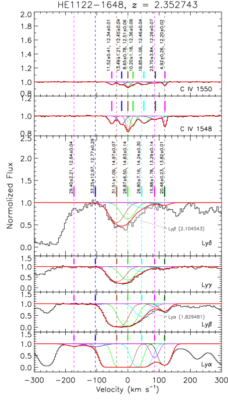
Figure 12: Example of a velocity plot (a relative velocity vs normalised absorption profile plot) of H i and associated C iv detected in the $z=2.352743$ absorber in the spectrum of HE1122$-$1648. The strongest C iv component is set to be at the zero velocity. The observed spectra are plotted as a histogram, while Voigt-profile fits are as a smooth curve. Thick red curves are the combined fit from individual components. The heavy tick marks above the profiles indicate the velocity centroid of each component. Non-negligible blends by other ions are indicated in gray. The $b$ value (in km s^-1) and $\log N_{{H\textsc{i}}}$ with the VPFIT fitting errors are displayed next a tick mark indicating the center of the component.

5.1 Method

Unfortunately there is no one-to-one relation between H i lines and C iv lines. Fig. 12 shows a velocity plot (the relative velocity centered at the redshift of an absorber vs normalised flux) of a typical C iv-enriched H i absorber in the spectrum of HE1122$-$1648. The vertical dashed lines indicate the velocity of individual H i components. Not all H i lines can be directly assigned to one or only one C iv component. For example, the H i component at $-36.02$ km s^-1 could be associated either with the first C iv component at $-51.72$ km s^-1 or with the second one at $-19.97$ km s^-1, or with both. A general trend is that the associated C iv features show an increased number of velocity components as $N_{\mathrm{{H\textsc{i}}}}$ increases. The absorption line centers of H i and C iv lines often show velocity differences as well, indicating that the H i-absorbing gas might not be co-spatial with the C iv-producing gas. Therefore, we apply a simple assigning method to our fitted absorber line lists, in order to determine if an H i absorption line is associated with C iv.

We consider an H i absorber to be metal enriched if a C iv line with $N_{\mathrm{{C\textsc{iv}}}}$ greater than a threshold value exists within the velocity range $\pm\Delta v_{\mathrm{{C\textsc{iv}}}}$ centered at each identified H i line. The threshold $N_{\mathrm{{C\textsc{iv}}}}$ should be large enough not to be affected by the incompleteness of weak C iv detection, but not too large so that there are enough C iv enriched absorbers to have a meaningful statistics. This method can assign one H i component with multiple C iv components and vice versa. As we are not concerned with the one-to-one relation between $N_{\mathrm{{C\textsc{iv}}}}$ and $N_{\mathrm{{H\textsc{i}}}}$ of each H i component, but the existence of the C iv line for a given search velocity range, the multiple assigning of the same component does not affect the results.

Two arbitrary choices of $\Delta v_{\mathrm{{C\textsc{iv}}}}$ are considered: a conservative narrow range of $\pm 10\textrm{ km s}^{-1}$ (a minimum $b$ value of a single Ly$\alpha$ absorption line is roughly 20 km s^-1) and a more generous interval of $\pm 100\textrm{ km s}^{-1}$.

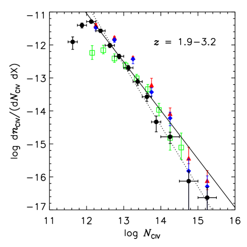
Figure 13: The C iv column density distribution. Filled circles are our results at the redshift range used for the high-order fit C iv-enriched H i sample at $1.9\!<\!z\!<\!3.2$. The CCD gap in the C iv region was accounted for. Red filled triangles and blue filled diamonds are from Pichon et al. (2003) at $1.5\!<\!z\!<\!2.3$ and $2.3<z<3.1$, respectively. Green open squares are taken from Songaila (2001) at $2.90<z<3.54$. The vertical error bars indicate $1\sigma$ Poisson errors, while the x-axis error bars show the $N_{\mathrm{{H\textsc{i}}}}$ range covered by each data point. The black dotted line shows the linear regression to filled circles at $\log N_{\mathrm{{C\textsc{iv}}}}=[12.25,15.5]:\log\mathrm{d}n_{\mathrm{{C\textsc{iv}}}}/(\mathrm{d}N_{\mathrm{{C\textsc{iv}}}}\mathrm{d}X)=(11.41\pm 1.61)+(-1.85\pm 0.13)\times\log N_{\mathrm{{C\textsc{iv}}}}$. The solid line is the power law fit at $\log N_{\mathrm{{C\textsc{iv}}}}=[12.25,13.5]:\log\mathrm{d}n_{\mathrm{{C\textsc{iv}}}}/(\mathrm{d}N_{\mathrm{{C\textsc{iv}}}}\mathrm{d}X)=(6.60\pm 1.23)+(-1.47\pm 0.10)\times\log N_{\mathrm{{C\textsc{iv}}}}$. The turn-over at $\log N_{\mathrm{{C\textsc{iv}}}}\!\sim\!12.5$ shown in green data is simply due to the incompleteness for weak C iv. Similarly, the turn-over seen at $\log N_{\mathrm{{C\textsc{iv}}}}\!\sim\!12.1$ in our data is also due to the incompleteness.

Fig. 13 shows the C iv column density distribution function at $1.9\!<\!z\!<\!3.2$ from our sample (black filled circles). For comparison, other results from the literature are also included: red filled triangles and blue filled diamonds from Pichon et al. (2003) at $1.5\!<\!z\!<\!2.3$ and $2.3\!<\!z\!<\!3.1$, respectively, and green open squares from Songaila (2001) at $2.90\!<\!z\!<\!3.54$. The turn-over seen in green open squares is due to the incompleteness effect, i.e. not all weak C iv can be detected due to noise.

Similar to the H i density distribution, the C iv CDDF does not fit with a single power law over a large $N_{\mathrm{{C\textsc{iv}}}}$ range. The Pichon et al. result even suggests that the C iv density distribution might have a non-linear functional form. At $\log N_{\mathrm{{C\textsc{iv}}}}=[12.25,13.5]$, a single power-law fit gives $\log\mathrm{d}N/(\mathrm{d}N_{\mathrm{{C\textsc{iv}}}}\mathrm{d}X)=(6.60\pm 1.23)+(-1.47\pm 0.10)\times\log N_{\mathrm{{C\textsc{iv}}}}$ (the solid line). At $\log{\mathrm{{C\textsc{iv}}}}=[12.25,15.5]$, a single power law is $\log\mathrm{d}N/(\mathrm{d}N_{\mathrm{{C\textsc{iv}}}}\mathrm{d}X)=(11.41\pm 1.61)+(-1.85\pm 0.13)\times\log N_{\mathrm{{C\textsc{iv}}}}$ (the dotted line). If the solid line is taken as a reasonable CDDF since it fits the low-$N_{\mathrm{{C\textsc{iv}}}}$ CDDF better, our C iv detection can be considered complete at $\log N_{\mathrm{{C\textsc{iv}}}}\!\geq\!12.2$.

Another way to look at whether our $N_{\mathrm{{C\textsc{iv}}}}$ completeness limit is reasonable is with the column density–$b$ value diagram. As seen in the 7th column of Table 1, the S/N differs for different sightlines, and changes even along a single spectrum. This makes it extremely difficult to quantify the correct 3$\sigma$ detection limit for a dataset containing spectra with different S/N.

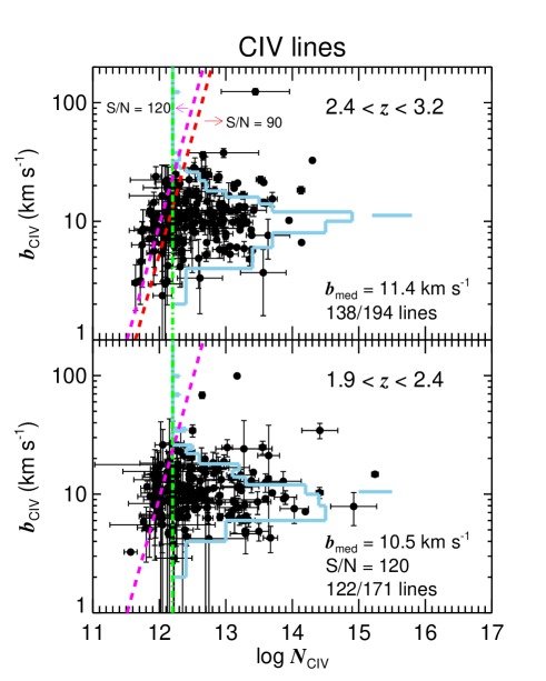
Figure 14: Line width vs. column density for the C iv absorption lines along 16 sightlines excluding Q0055$-$269 and J2233$-$606 at the two redshift bins. Error bars are fitting errors from the VPFIT profile fitting. In the upper panel, two heavy dashed lines delineate a 3$\sigma$ detection limit for a spectrum with S/N $=120$ and S/N $=90$ per pixel. At $2.4<z<3.2$, most spectra show S/N greater than 90. In the lower panel, the heavy dashed line shows a 3$\sigma$ detection limit for S/N $=120$. Broader and weaker absorption lines at the left of the detection limit are missed in lower S/N spectra. The vertical dotted line indicates the adopted low $N_{\mathrm{{C\textsc{iv}}}}$ bound of $\log N_{\mathrm{{C\textsc{iv}}}}\!=\!12.2$ above which the incompleteness does not affect the C iv detection significantly. The histogram shown with the base at $\log N_{\mathrm{{C\textsc{iv}}}}\!=\!12.2$ is the number of C iv lines as a function of $b_{\mathrm{{C\textsc{iv}}}}$ with the $b_{\mathrm{{C\textsc{iv}}}}$ binsize of 2 km s^-1. Thick ticks above the number distribution mark the median $b_{\mathrm{{C\textsc{iv}}}}$ for $\log N_{\mathrm{{C\textsc{iv}}}}\!\geq\!12.2$. The total number of C iv lines is 194 and 171 at $2.4<z<3.2$ and $1.9<z<2.4$, respectively. Among them, 138 and 122 lines have $\log N_{\mathrm{{C\textsc{iv}}}}\!\geq\!12.2$ at the same redshift range.

Fig. 14 shows the $\log N_{\mathrm{{C\textsc{iv}}}}$–$b_{\mathrm{{C\textsc{iv}}}}$ diagram at the two redshift bins. The vertical heavy dot-dashed lines mark $\log N_{\mathrm{{C\textsc{iv}}}}=12.2$. In the upper panel, two heavy dashed lines show a 3$\sigma$ detection limit for a spectrum with S/N $=120$ (the left side) and 90 (the right side, an approximate lowest S/N) per pixel, respectively. In the lower panel, the heavy dashed line is a 3$\sigma$ detection limit for S/N $=120$. Absorption lines at the left-side of the detection limit, i.e. broader and weaker lines, can be only detected for S/N greater than the given S/N. Overlaid as a histogram is the distribution of the number of C iv lines with $\log N_{\mathrm{{C\textsc{iv}}}}\!\geq\!12.2$ as a function of $b_{\mathrm{{C\textsc{iv}}}}$. For the distribution, the zero base is set to be $\log N_{\mathrm{{C\textsc{iv}}}}=12.2$. Thick ticks above the distribution mark the median $b_{\mathrm{{C\textsc{iv}}}}$. There is no correlation between $N_{\mathrm{{C\textsc{iv}}}}$ and $b_{\mathrm{{C\textsc{iv}}}}$ above the S/N detection limit at all of the reasonable expected $b_{\mathrm{{C\textsc{iv}}}}$ values.

At $2.4<z<3.2$ (the upper panel), the 3$\sigma$ $b_{\mathrm{{C\textsc{iv}}}}$ detection limit is 23.6 (13.4) km s^-1 for S/N $=120$ (90) at $\log N_{\mathrm{{C\textsc{iv}}}}\!\sim\!12.2$. The total wavelength coverage of C iv at the high redshift bin is $\sim\!3192$ Å. For about half of the spectra there is contamination from weak telluric lines in $\leq\!10$% of the C iv region. This contamination prevents isolated weak C iv lines from being detected, however, can be treated as a lower-S/N region. Including the telluric-contaminated region, the wavelength coverage with S/N $\leq\!120$ is about 1018 Å. In the C iv wavelength region with S/N $\geq\!120$, the total number of C iv lines with $\log N_{\mathrm{{C\textsc{iv}}}}=[12.2,12.3]$ is 8. Out of those 8, none has $b_{\mathrm{{C\textsc{iv}}}}\!\geq\!23.6$ km s^-1. It is possible that a large fraction of C iv has a $b_{\mathrm{{C\textsc{iv}}}}$ value greater than 23.6 km s^-1, and therefore, would be completely missed even in the high-S/N spectra analysed here. However, as clearly seen in the upper panel of Fig. 14, the $b_{\mathrm{{C\textsc{iv}}}}$ distribution at $\log N_{\mathrm{{C\textsc{iv}}}}\!\geq\!12.2$ shows that only 9% of C iv has $b_{\mathrm{{C\textsc{iv}}}}\!\geq\!23.6$ km s^-1. If a large fraction of C iv lines were broader regardless of $N_{\mathrm{{C\textsc{iv}}}}$, the region around $\log N_{\mathrm{{C\textsc{iv}}}}\!\sim\!12.4$ and $b_{\mathrm{{C\textsc{iv}}}}\!\sim\!25$ km s^-1 in Fig. 14 should have been more crowded. Therefore, it is not likely that many weak C iv lines with $b_{\mathrm{{C\textsc{iv}}}}\!\geq\!23.6$ km s^-1 have been missed for S/N $\geq\!120$.

Only 2 out of 8 have $b_{\mathrm{{C\textsc{iv}}}}\!\geq\!13.4$ km s^-1 at $\log N_{\mathrm{{C\textsc{iv}}}}=[12.2,12.3]$. In other words, these 2 C iv lines would have been missed in the S/N $\leq\!120$ region. One is a single isolated line, while the other is part of a multi-component C iv complex. We assumed that the number of C iv lines with $\log N_{\mathrm{{C\textsc{iv}}}}\!\sim\!12.2$ and $b_{\mathrm{{C\textsc{iv}}}}\!\geq\!13.4$ km s^-1 is 2 in the wavelength range of 2174 Å, i.e. the total wavelength range with S/N $\geq\!120$. If we assume that weak C iv lines have a negligible clustering, about 1 (or $2\times 1018/(3192-1018)=0.9$) C iv line with $\log N_{\mathrm{{C\textsc{iv}}}}\!\sim\!12.2$ and $b_{\mathrm{{C\textsc{iv}}}}\!\geq\!13.4$ km s^-1 could have been missed in the C iv forest region with S/N $\leq\!120$.

A total of 5 H i lines with $\log N_{\mathrm{{H\textsc{i}}}}\!=\![12.8,17.5]$ is found within $\pm$100 km s^-1 centered at these two C iv lines. The total number of high-order-fit H i lines in the H i forest region corresponding to the S/N $\!\geq\!120$ C iv forest region is [265, 363, 233, 120, 50, 27, 5] for $\log N_{\mathrm{{H\textsc{i}}}}\!=\!$ [12.75–13.00, 13.0–13.5, 13.5–14.0, 14.0–14.5, 14.5–15.0, 15.0–16.0, 16.0–17.0], respectively. Among them, a negligible number of H i lines, [0, 0, 2, 0, 1, 0, 1], is associated with these two C iv lines for the same $N_{\mathrm{{H\textsc{i}}}}$ range, or less than 2%. The remaining one H i line has $\log N_{\mathrm{{H\textsc{i}}}}\!\geq\!17.0$ as the associated C iv line belongs to a C iv complex of a partial Lyman limit system. Although the number of undetected weak and broad C iv lines in the S/N $\leq\!120$ region is a very rough estimate, less than 2% of the H i lines would be mis-classified as the unenriched forest due to the incompleteness at $\log N_{\mathrm{{C\textsc{iv}}}}\!\sim\!12.2$.

The situation becomes more complicated in the low redshift bin, where the variance of the S/N limits of individual spectra is much higher than in the high redshift bin. If a similar logic were applied to, the total C iv coverage is 5485 Å, and the one with S/N $\!\leq\!120$ is 2719 Å. In the S/N $\!\geq\!120$ C iv region, there is a total of 10 C iv lines with $\log N_{\mathrm{{C\textsc{iv}}}}=[12.2,12.3]$. Out of 10, 6 lines have $b_{\mathrm{{C\textsc{iv}}}}\!\geq\!13.4$ km s^-1, the maximum $b_{\mathrm{{C\textsc{iv}}}}$ value to be detected for a line with $\log N_{\mathrm{{C\textsc{iv}}}}=[12.2,12.3]$ in a S/N $=90$ spectrum. Among those 6 C iv lines, two C iv lines are part of a two-isolated-component complex, with the rest being part of a multi-component complex. Since stronger H i lines tend to be associated with a C iv complex, using all these 6 C iv lines to calculate the associated H i fraction leads to a biased result. Therefore, we used 4 C iv lines which are part of a C iv complex with less than 3 components in order to estimate the missed enriched H i fraction.

There is a total of 11 H i lines at $\log N_{\mathrm{{H\textsc{i}}}}=[12.75,16.00]$ within 100 km s^-1 centered at the 4 weak C iv lines. The ratio of the C iv enriched H i lines and the total H i lines in the wavelength regions corresponding to the S/N $\geq\!120$ C iv forest is [2/231, 4/315, 3/174, 1/59, 1/28, 0/10] for $\log N_{\mathrm{{H\textsc{i}}}}\!=\!$ [12.75–13.00, 13.0–13.5, 13.5–14.0, 14.0–14.5, 14.5–15.0, 15.0–16.0], respectively, or $\leq\!3$%. Again the fraction of missed C iv is negligible even at the low redshift bin.

Note that our estimate on the true undetected C iv fraction is uncertain. However, from Fig. 13, the incompleteness at $\log N_{\mathrm{{C\textsc{iv}}}}=12.2$ is less than 10% or within the 1$\sigma$ Poisson error.

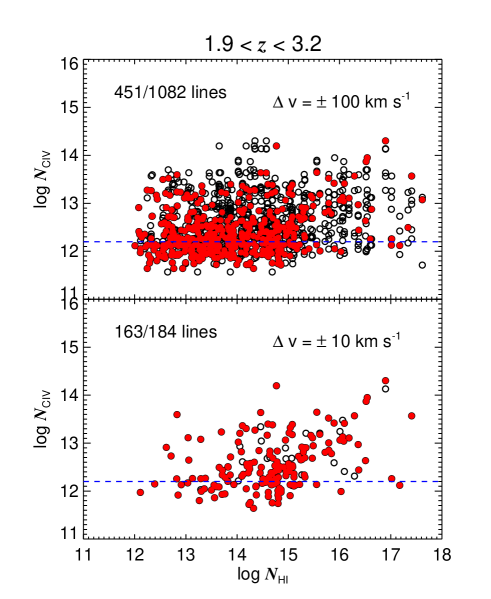
Figure 15: The $N_{\mathrm{{H\textsc{i}}}}$–$N_{\mathrm{{C\textsc{iv}}}}$ diagram for $\log N_{\mathrm{{H\textsc{i}}}}=[12.0,17.8]$ from the high-order fit sample at $1.9\!<\!z\!<\!3.2$. The upper panel is for the $\Delta v_{\mathrm{{C\textsc{iv}}}}=\pm 100\textrm{ km s}^{-1}$ sample, while the lower panel for the $\Delta v_{\mathrm{{C\textsc{iv}}}}=\pm 10\textrm{ km s}^{-1}$ sample. Open circles represent H i absorbers associated with all the possible C iv components, since a single H i line could be assigned to several C iv lines. On the other hand, red filled circles indicate a H i absorber associated with only one closest C iv. The total number of open (filled) circles is 1082 (451) and 184 (163) for the $\Delta v_{\mathrm{{C\textsc{iv}}}}=\pm 100\textrm{ km s}^{-1}$ and $\Delta v_{\mathrm{{C\textsc{iv}}}}=\pm 10\textrm{ km s}^{-1}$ sample, respectively.

While it is clear that the incompleteness does not play a significant role in the H i detection down to $\log N_{\mathrm{{H\textsc{i}}}}=12.75$ and the C iv detection down to $\log N_{\mathrm{{C\textsc{iv}}}}=12.2$, the combination of the H i and C iv detection could introduce a bias in the C iv assigning method. The pixel optical depth method which correlates the optical depth of H i ($\tau_{\mathrm{{H\textsc{i}}}}$) and C iv ($\tau_{\mathrm{{C\textsc{iv}}}}$) at the same redshift shows that at $z\sim 3$ there is a one-to-one positive correlation between the median $\tau_{\mathrm{{H\textsc{i}}}}$ and the median $\tau_{\mathrm{{C\textsc{iv}}}}$ down to $\log\tau_{\mathrm{{H\textsc{i}}}}\!\sim\!0.15$ or $\log N_{\mathrm{{H\textsc{i}}}}\!\sim\!13.73$ for $b_{\mathrm{{H\textsc{i}}}}=28$ km s^-1 (a median $b_{\mathrm{{H\textsc{i}}}}$ of the forest at $z\!\sim\!2.5$) (Schaye et al. 2003). Below $\log\tau_{\mathrm{{H\textsc{i}}}}\!\sim\!0.15$, the $\tau_{\mathrm{{H\textsc{i}}}}$ signal is blended with noise at $\log\tau_{\mathrm{{C\textsc{iv}}}}\!\sim\!0.001$ or $\log N_{\mathrm{{C\textsc{iv}}}}\!\leq\!11.0$ for $b_{\mathrm{{C\textsc{iv}}}}=9.5$ km s^-1 (a median $b_{\mathrm{{C\textsc{iv}}}}$ of all the C iv lines in our UVES sample).

This result suggests that many low-$N_{\mathrm{{H\textsc{i}}}}$ absorbers might be mis-assigned as unenriched H i absorber in our C iv assigning method. Unfortunately, the lower $\log N_{\mathrm{{C\textsc{iv}}}}\!\sim\!11$ limit that a typical optical depth analysis explores is an order of magnitude lower than our adopted low $N_{\mathrm{{C\textsc{iv}}}}$ limit of $\log N_{\mathrm{{C\textsc{iv}}}}=12.2$. This $\log N_{\mathrm{{C\textsc{iv}}}}\!\sim\!11$ limit cannot be obtained even in the highest S/N C iv region with S/N $\geq\!220$ in our UVES spectra. Therefore, our C iv analysis can not confirm, nor refute the results from the optical depth method.

Fig. 15 shows the $N_{\mathrm{{H\textsc{i}}}}$–$N_{\mathrm{{C\textsc{iv}}}}$ diagram for the $\Delta v_{\mathrm{{C\textsc{iv}}}}=\pm 100\textrm{ km s}^{-1}$ sample (the upper panel) and for the $\Delta v_{\mathrm{{C\textsc{iv}}}}=\pm 10\textrm{ km s}^{-1}$ sample (the lower panel). Since one H i line can be associated with several C iv lines, data points at the same $N_{\mathrm{{H\textsc{i}}}}$ represent the same H i absorber. Open circles show all the H i absorbers associated with all the possible C iv lines. Red filled circles indicate H i absorbers associated with only one closest C iv within the search velocity range. With a larger search velocity range, the $\Delta v_{\mathrm{{C\textsc{iv}}}}=\pm 100\textrm{ km s}^{-1}$ sample has more lines. The number of the red filled circles increases abruptly at $\log N_{\mathrm{{H\textsc{i}}}}\leq 15.0$ at both redshift ranges, more prominently at the high redshift bin. This is simply due to the fact that the number of weaker H i absorbers is larger than stronger H i absorbers.

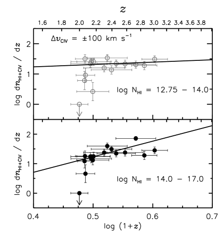
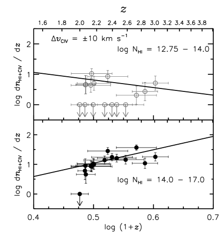
Figure 16: Quasar by quasar line number density evolution of C iv-enriched H i absorbers. The left panels are derived from the $\Delta v_{\mathrm{{C\textsc{iv}}}}=\pm 100\textrm{ km s}^{-1}$ sample, while the right panels represent the $\Delta v_{\mathrm{{C\textsc{iv}}}}=\pm 10\textrm{ km s}^{-1}$ one. The open circles in the upper panel represent C iv-enriched absorbers having $\log N_{H\textsc{i}}=[12.75,14.0]$ and the filled circles in the lower panel represent $\log N_{H\textsc{i}}=[14,17]$. The vertical error bars mark $1\sigma$ Poisson errors, while the x-axis error bars show the redshift range covered by each sightline. Sightlines having no C iv-enriched H i absorbers for a given velocity range are plotted at $\log\mathrm{d}dn_{\mathrm{{C\textsc{iv}}}}/\mathrm{d}dz=0$. The solid lines represent linear regressions to the data, using the parameters summarised in Table 4. Sightlines with no C iv-enriched absorbers, $\log\mathrm{d}n_{{H\textsc{i}}+{C\textsc{iv}}}/\mathrm{d}z$ is plotted to be 0 with a downward arrow.

If our C iv assigning method were biased due to our failure to detect C iv lines toward lower $N_{\mathrm{{H\textsc{i}}}}$ values, there should be a correlation in $N_{\mathrm{{H\textsc{i}}}}$ and $N_{\mathrm{{C\textsc{iv}}}}$, such that a lower $N_{\mathrm{{H\textsc{i}}}}$ line tends to be associated with a lower $N_{\mathrm{{C\textsc{iv}}}}$ line (cf. the relation between the median $\tau_{\mathrm{{H\textsc{i}}}}$ and the median $\tau_{\mathrm{{C\textsc{iv}}}}$) or the number of the C iv-enriched H i lines at lower $N_{\mathrm{{H\textsc{i}}}}$ is smaller. No such correlations are seen in Fig. 15. Note that our method deals with the fitted individual lines, while the optical depth analysis works with statistical, median values. The optical depth analysis is not sensitive to any minor C iv population, such as high-metallicity absorbers (Schaye et al. 2007).

In reality, the detection of weak C iv is dependent on the local S/N as well as the combination of $b_{\mathrm{{C\textsc{iv}}}}$ and $N_{\mathrm{{C\textsc{iv}}}}$. The S/N of a spectrum does not change in a way to satisfy a higher S/N at strong H i absorbers and a lower S/N at weaker H i absorbers or vice versa. Usually the S/N changes over a larger wavelength interval than the wavelength interval between typical strong H i lines. In addition, strong and weak H i lines do not occupy a portion of a spectrum separately, but exist mixed along the spectrum. If a weak C iv were detected associated with a high-$N_{\mathrm{{H\textsc{i}}}}$ line, a similar strength of C iv, if exists, should be detected for low-$N_{\mathrm{{H\textsc{i}}}}$ lines nearby or in a similar S/N region. Therefore, unless a majority C iv fraction at lower $N_{\mathrm{{C\textsc{iv}}}}$ and/or lower $N_{\mathrm{{H\textsc{i}}}}$ has a very large $b_{\mathrm{{C\textsc{iv}}}}$ value, i.e. high gas temperature, our C iv assigning method does not introduce a serious selection bias within the adopted $N_{\mathrm{{C\textsc{iv}}}}$ limit.

5.2 Results

5.2.1 Number density evolution of the C iv-enriched absorbers

In a similar way to the analysis of all the H i absorbers, we calculate the absorber number density evolution $\mathrm{d}n_{{H\textsc{i}}+{C\textsc{iv}}}/\mathrm{d}z$ on a quasar by quasar analysis for all the C iv-enriched H i absorbers. The resulting $\mathrm{d}n_{{H\textsc{i}}+{C\textsc{iv}}}/\mathrm{d}z$ evolution is shown in Fig. 16 for the $\Delta v_{\mathrm{{C\textsc{iv}}}}=\pm 100\textrm{ km s}^{-1}$ and $\Delta v_{\mathrm{{C\textsc{iv}}}}=\pm 10\textrm{ km s}^{-1}$ interval from the high-order Lyman fit samples. For the $\Delta v_{\mathrm{{C\textsc{iv}}}}=\pm 100\textrm{ km s}^{-1}$ sample, the Q1101$-$264 sightline does not show any C iv in the redshift range of interest due to its short redshift coverage. For the $\Delta v_{\mathrm{{C\textsc{iv}}}}=\pm 10\textrm{ km s}^{-1}$ sample, 7 sightlines (HE2347$-$4342, Q0002$-$422, PKS0329$-$255, HE1347$-$2457, Q0109$-$3518, Q0122$-$380 and Q1101$-$264) out of 16 have no C iv-enriched H i absorbers at $\log N_{\mathrm{{H\textsc{i}}}}=[12.75,14.0]$, while only only sightline (Q1101$-$264) has no C iv-enriched H i absorber at $\log N_{\mathrm{{H\textsc{i}}}}=[14,17]$. This is caused by the combination of two facts that C iv tends to be associated with strong H i absorbers and that the small search velocity is not adequate due to the velocity difference between H i and C iv observed in many enriched absorbers. For these sightlines, $\mathrm{d}n_{{H\textsc{i}}+{C\textsc{iv}}}/\mathrm{d}z$ is 0. Therefore, their $\log n_{{H\textsc{i}}+{C\textsc{iv}}}/\mathrm{d}z$ is set to be 0 with a downward arrow in Fig. 16.

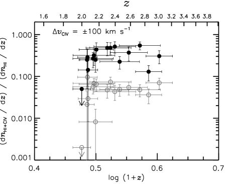
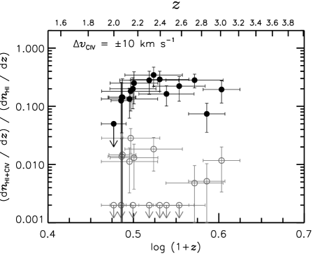
Figure 17: The fraction of the C iv-enriched H i absorber number density to the total absorber number density as a function of redshift. The left panels are derived from the $\Delta v_{\mathrm{{C\textsc{iv}}}}=\pm 100\textrm{ km s}^{-1}$ sample, while the right panels represent the $\Delta v_{\mathrm{{C\textsc{iv}}}}=\pm 10\textrm{ km s}^{-1}$ sample. The black open circles represent a column density interval of $\log N_{H\textsc{i}}=[12.75,14.0]$ and the filled circles represent $\log N_{H\textsc{i}}=[14,17]$. The vertical error bars mark $1\sigma$ Poisson errors, while the x-axis error bars show the redshift range covered by each sightline. In the left panel for $\log N_{H\textsc{i}}=[12.75,14.0]$ (gray open circles), two lowest data points at $\log(1+z)\sim 0.5$ (or $z\sim 2$) including an upper limit are from Q1101$-$264 and Q0122$-$380. Both have a short redshift coverage, therefore become more susceptible to cosmic variance. Sightlines with no C iv-enriched H i absorbers are plotted as upper limits with an arbitrary value of 0.05 and 0.002 for $\log N_{H\textsc{i}}=[14,17]$ and $\log N_{H\textsc{i}}=[12.75,14.0]$, respectively.

As for the entire Ly$\alpha$ forest analysis, the $\mathrm{d}n_{{H\textsc{i}}+{C\textsc{iv}}}/\mathrm{d}z$ evolution resembles a power law. Therefore, linear regressions have been obtained from the data set and its results are summarised in Table 4. Sightlines showing no C iv-enriched H i absorbers were not included in the regression. Similar to the entire high-order-fit H i sample, the $\Delta v_{\mathrm{{C\textsc{iv}}}}=\pm 100\textrm{ km s}^{-1}$ sample shows a decline in the C iv-enriched absorber number density with decreasing redshift. This behaviour is present in both column density ranges. Comparing these results with the quasar-by-quasar $\mathrm{d}n/\mathrm{d}z$ of the entire high-order fit sample at $1.9<z<3.2$ shows that the C iv-enriched absorbers at $\log N_{H\textsc{i}}=[14,17]$ has a steeper slope ($5.27\pm 0.99$), but completely consistent within 1$\sigma$. The robust result on the $\mathrm{d}n_{{H\textsc{i}}+{C\textsc{iv}}}/\mathrm{d}z$ evolution requires a large redshift coverage and more sightlines per redshift coverage, especially at high column density range. With a lack of more C iv forest data at $z_{\mathrm{forest}}>3$, $\mathrm{d}n_{{H\textsc{i}}+{C\textsc{iv}}}/\mathrm{d}z$ derived in this study at the high column density range should be considered less robust compared to the entire H i $\mathrm{d}n/\mathrm{d}z$. Similarly, the $\mathrm{d}n_{{H\textsc{i}}+{C\textsc{iv}}}/\mathrm{d}z$ slope ($0.78\pm 0.92$) at $\log N_{H\textsc{i}}=[12.75,14.0]$ is also consistent with the one ($1.38\pm 0.22$) of the entire high-order-fit forest sample, given the rather large uncertainty. The actual number densities are lower at both column density ranges.

This becomes apparent in the left panel of Fig. 17, where the ratios of the number densities of the C iv-enriched systems $\mathrm{d}n_{{H\textsc{i}}+{C\textsc{iv}}}/\mathrm{d}z$ and the number density of the entire sample $\mathrm{d}n/\mathrm{d}z$ are shown. The results for the $\Delta v_{\mathrm{{C\textsc{iv}}}}=\pm 100\textrm{ km s}^{-1}$ sample (filled circles) show that there is no significant evolution of the C iv enrichment fraction for $\log N_{H\textsc{i}}=[12.75,14.0]$. For $\log N_{H\textsc{i}}=[14,17]$, the enrichment fraction is consistent with no redshift evolution, considering a large scatter at $z\sim 2$ and a lack of data at $z>3$. For the low column density $\log N_{H\textsc{i}}=[12.75,14.0]$ sample we find that around 5% of all the H i absorbers show C iv enrichment. The C iv enrichment fraction is higher for larger column densities of $\log N_{H\textsc{i}}=[14,17]$, where around 40% of the absorbers are C iv-enriched.

Table 4: Linear regression results for the number density evolution $\mathrm{d}n_{{H\textsc{i}}+{C\textsc{iv}}}/\mathrm{d}z$ of the C iv-enriched H i forest absorbers in the quasar by quasar analysis.

	$\Delta v_{\mathrm{{C\textsc{iv}}}}=\pm 100\textrm{ km s}^{-1}$		$\Delta v_{\mathrm{{C\textsc{iv}}}}=\pm 10\textrm{ km s}^{-1}$
$\Delta\log N_{H\textsc{i}}$	$\log A$	$\gamma$	$\log A$	$\gamma$
$12.75-14.0$	$0.92\pm 0.49$	$0.78\pm 0.92$	$2.06\pm 1.02$	$-2.49\pm 1.94$
$14.0-17.0$	$-1.40\pm 0.53$	$5.27\pm 0.99$	$-1.22\pm 0.64$	$4.52\pm 1.22$

This picture changes slightly for the $\Delta v_{\mathrm{{C\textsc{iv}}}}=\pm\,10\textrm{ km s}^{-1}$ sample. For the high column densities, the $\mathrm{d}n_{{H\textsc{i}}+{C\textsc{iv}}}/\mathrm{d}z$ evolution is less strong compared to the one of the $\Delta v_{\mathrm{{C\textsc{iv}}}}=\pm 100\textrm{ km s}^{-1}$ sample. However, both are still consistent within 1$\sigma$ due to a large uncertainty. Only the number density itself decreases by a factor of 1.7. The enrichment fractions in the right panel of Fig. 17 show that now around 20% to 30% of the high column density H i absorbers are C iv-enriched.

On the other hand, $\mathrm{d}n_{{H\textsc{i}}+{C\textsc{iv}}}/\mathrm{d}z$ increases with decreasing redshift for the low column densities. Its negative slope of $\gamma=-2.49\pm 1.94$ shows an opposite behaviour from the one ($\gamma=0.78\pm 0.92$) of the $\Delta v_{\mathrm{{C\textsc{iv}}}}=\pm 100\textrm{ km s}^{-1}$ sample. This negative slope is in part caused by the inadequacy in our C iv assigning method at the small search velocity, and in part by the fact that the number of high-metallicity absorbers increases at low redshift (Schaye et al. 2007). However, due to several sightlines containing no C iv-enriched weak H i absorbers which are not included in the power-law fit, the negative slope should not be taken literally. The fraction of enriched absorbers increases from $\sim$0.5% at $z\sim 3$ to $\sim$1.5% at $z\sim 2.1$, as expected from $\mathrm{d}n_{{H\textsc{i}}+{C\textsc{iv}}}/\mathrm{d}z$ at the low H i column density. However, keep in mind that the cosmic variance is large as some sightlines show no enriched weak H i absorbers.

There are two distinct groups of C iv absorbers assigned to the low H i column density. One group is associated with strong, saturated high column density H i absorbers. These absorbers are sometimes accompanied by lower $N_{\mathrm{{H\textsc{i}}}}$ absorbers within a velocity range of $\Delta v<200\textrm{ km s}^{-1}$. In these systems, the C iv absorption is usually found within $20\textrm{ km s}^{-1}$ to the strongest H i lines (Kim et al. 2013, in preparation). Therefore, these accompanied low H i column density systems get associated with the C iv absorbers if the velocity range $\Delta v_{\mathrm{{C\textsc{iv}}}}$ is large. With a small velocity search interval, however, only H i systems that have C iv in their direct vicinity are flagged as C iv-enriched. This means that the aforementioned low column density systems around strong absorbers are not considered C iv-enriched in a small velocity search interval.

Another C iv-enriched group consists of usually isolated, low column density H i absorbers associated with strong C iv absorption, i.e. the same high-metallicity forest population studied by Schaye et al. (2007). An example of such a system toward HE1122$-$1648 is shown in Fig. 18. In this velocity plot, an H i absorption feature is hardly recognisable, while strong C iv and N v doublets are present. The existence of both doublets makes the identification of this absorber secure. Due to the low $N_{\mathrm{{H\textsc{i}}}}$ and high $N_{\mathrm{metals}}$, these systems show a higher ionisation and a higher metallicity compared to a typical absorber with similar $N_{\mathrm{{H\textsc{i}}}}$ (Carswell et al. 2002; Schaye et al. 2007). Schaye et al. (2007) speculate that these systems could be responsible for transporting metals from galaxies to the surrounding IGM. As the velocity difference between H i and metal lines for these systems are usually very small, they dominate the weaker C iv-enriched forest at $\log N_{\mathrm{{H\textsc{i}}}}\!<\!14$ for the $\Delta v_{\mathrm{{C\textsc{iv}}}}=\pm 10\textrm{ km s}^{-1}$. In addition, the high-metallicity absorbers are more common at low redshift.

Figure 18: A velocity plot of a highly enriched C iv absorber at $z=2.030069$ toward HE1122$-$1648. The zero velocity is centered at $z=2.030069$. Although there is no obvious Ly$\alpha$ absorption seen at the zero velocity, both C iv and N v doublets are present to secure the existence of this absorber. Note that the y-axis range for each ion is different: from the normalised flux 0 to 1 for H i and from 0.5 to 1 for the rest of the ions.

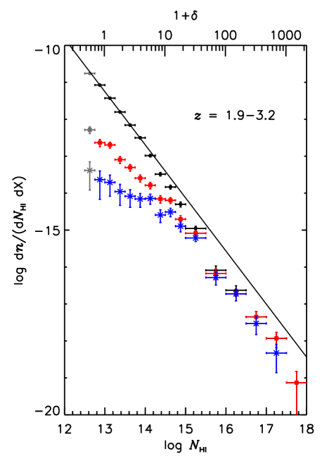
Figure 19: The distribution function for C iv-enriched H i lines for $\Delta v_{\mathrm{{C\textsc{iv}}}}=\pm 100\textrm{ km s}^{-1}$ (red filled squares) and for $\Delta v_{\mathrm{{C\textsc{iv}}}}=\pm 10\textrm{ km s}^{-1}$ (blue stars) at $1.9\!<\!z\!<\!3.2$. Also shown is the differential column density distribution function for all H i Ly$\alpha$ absorbers excluding Q0055$-$269 and J2233$-$606 (black filled circles) in the same redshift range analysed for the C iv-enriched forest. The solid line indicates the fit to filled circles for $\log N_{H\textsc{i}}=[12.75,14.0]:\log\mathrm{d}N/(\mathrm{d}N_{\mathrm{{H\textsc{i}}}}\mathrm{d}X)=(7.43\pm 0.44)+(-1.44\pm 0.03)\times\log N_{\mathrm{{H\textsc{i}}}}$. The vertical errors indicate $1\sigma$ Poisson errors, while the x-axis error bars show the $N_{\mathrm{{H\textsc{i}}}}$ range covered by each data point. All the grey data points indicate that the data are incomplete at $\log N_{H\textsc{i}}\!<\!12.75$.

The different characteristics of these two C iv groups explains the different $\mathrm{d}n_{C\textsc{iv}}/\mathrm{d}z$ behaviour between the $\Delta v_{\mathrm{{C\textsc{iv}}}}=\pm 100\textrm{ km s}^{-1}$ and $\Delta v_{\mathrm{{C\textsc{iv}}}}=\pm 10\textrm{ km s}^{-1}$ samples at $\log N_{\mathrm{{H\textsc{i}}}}=[12.75,14.0]$. With recent observational evidence that metals are only found close to galaxies in the circum-galactic medium at $2\!<\!z\!<\!4$ and not far away from galaxies (Adelberger et al. 2005; Steidel et al. 2010), our results could provide further theoretical constraints for this interpretation. It could well be that the high-metallicity forest population is completely different from the typical, low-metallicity forest and resides in a different intergalactic space. However, due to the low gas density and high temperature, the Ly$\alpha$ forest does not have in-situ star formation. Metals associated with the H i forest should have been transported from nearby galaxies. In other words, all the C iv-enriched absorbers are close to galaxies.

5.2.2 Differential column density distribution function of the C iv-enriched forest

Fig. 19 shows the differential column density distribution function for C iv-enriched H i absorbers for $1.9\!<\!z\!<\!3.2$. Red filled squares and blue stars represent the search velocity ranges of $\Delta v_{\mathrm{metal}}=\pm 100\textrm{ km s}^{-1}$ and $\Delta v_{\mathrm{metal}}=\pm 10\textrm{ km s}^{-1}$, respectively. Black filled circles are for all H i lines (excluding J2233$-$606 and Q0055$-$269), regardless of their metal association. As in Figs 7 and 10, the binsize of $\log N_{\mathrm{{H\textsc{i}}}}\!=\!0.25$ is used at $\log N_{\mathrm{{H\textsc{i}}}}\!=[12,15]$, then the binsize of 0.5 at $\log N_{\mathrm{{H\textsc{i}}}}\!=[15,18]$. The solid line indicates the fit to filled circles for $\log N_{H\textsc{i}}=[12.75,14.0]:\log\mathrm{d}N/(\mathrm{d}N_{\mathrm{{H\textsc{i}}}}\mathrm{d}X)=(7.43\pm 0.44)+(-1.44\pm 0.03)\times\log N_{\mathrm{{H\textsc{i}}}}$. The total absorption distance is $X(z)=19.6652$ for the redshift ranges analysed in this subsection.

For $\log N_{{H\textsc{i}}}\!>\!15$, the CDDF of the enriched forest is not sensitive to our choice of the search velocity and the $\Delta v_{\mathrm{metal}}=\pm 100\textrm{ km s}^{-1}$ CDDF becomes almost identical with the CDDF of the entire H i sample. For the column densities $\log N_{\mathrm{{H\textsc{i}}}}=[14,17]$, the CDDF functional form of the enriched forest shows a power-law with a similar slope obtained for the entire H i absorbers at $\log N_{\mathrm{{H\textsc{i}}}}=[12.75,14.0]$, but with a smaller normalisation value.

At $\log N_{H\textsc{i}}\!<\!15$, the distribution function of the C iv-enriched forest starts to deviate significantly from the CDDF of the entire H i sample. The CDDF of the C iv-enriched H i forest starts to flatten out toward lower $N_{\mathrm{{H\textsc{i}}}}$ at both search velocity ranges. Furthermore the flattening of the enriched forest depends strongly on the choice of $\Delta v_{\mathrm{{C\textsc{iv}}}}$. The large search velocity results in a steeper slope with a less fluctuation than the small one. This is due to the $\Delta v_{\mathrm{{C\textsc{iv}}}}=\pm 10\textrm{ km s}^{-1}$ sample being predominantly sensitive to highly enriched absorbers at $\log N_{H\textsc{i}}\!<\!14$ and less sensitive to mis-aligned broad C iv lines with $b\geq 10$ km s^-1. Note that our method to associate H i with C iv is only dependent on the relative velocity difference between the line centers, but not the C iv profile shape. The large velocity range includes broader C iv lines up to $b\!\sim\!100$ km s^-1 as well as narrow, highly enriched absorbers. The $\Delta v_{\mathrm{{C\textsc{iv}}}}=\pm 100\textrm{ km s}^{-1}$ velocity range is a better filter to associate H i and C iv.

The flattening of the distribution function seen at $\log N_{H\textsc{i}}\!<\!15$ by C iv-enriched absorbers cannot be caused by the incompleteness of the H i sample. The H i incompleteness would result in a similar flattening as is seen at $\log N_{H\textsc{i}}\!<\!12.75$ for the entire sample (as seen in Fig. 7). However, our sample of H i absorbers is complete for column densities larger than $\log N_{H\textsc{i}}\!>\!12.75$.

Table 5: Linear regression results for the differential column density distribution of the C iv-enriched forest at $\log N_{\mathrm{{H\textsc{i}}}}\!=\![14.5,17.0]$. Here the normalisation point $\log\left(\mathrm{d}n/(\mathrm{d}N_{H\textsc{i}}\,\mathrm{d}X)\right)_{0}$ is denoted by $B$.

	$\Delta v_{\mathrm{{C\textsc{iv}}}}=\pm 100\textrm{ km s}^{-1}$		$\Delta v_{\mathrm{{C\textsc{iv}}}}=\pm 10\textrm{ km s}^{-1}$
$z$	$B$	$\beta$	$B$	$\beta$
$1.9-3.2$	$6.93\pm 1.17$	$-1.45\pm 0.08$	$5.32\pm 1.50$	$-1.36\pm 0.10$
$1.9-2.4$	$5.94\pm 2.51$	$-1.40\pm 0.17$	$3.75\pm 3.26$	$-1.27\pm 0.21$
$2.4-3.2$	$6.90\pm 1.45$	$-1.44\pm 0.10$	$5.97\pm 1.94$	$-1.39\pm 0.13$

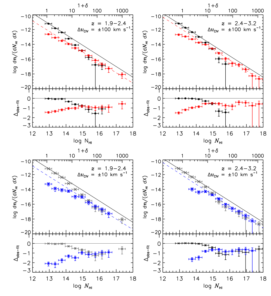
Figure 20: Differential column density distribution function for enriched and unenriched absorbers in our high-order fit sample using $\Delta v_{\mathrm{{C\textsc{iv}}}}\!=\!\pm 100\textrm{ km s}^{-1}$ (upper panels) and $\Delta v_{\mathrm{{C\textsc{iv}}}}\!=\!\pm 10\textrm{ km s}^{-1}$ (lower panels) at the two different redshift ranges. Black filled circles and gray stars mark unenriched absorbers. Red filled squares and blue stars indicate the C iv-enriched forest for the $\Delta v_{\mathrm{{C\textsc{iv}}}}\!=\!\pm 100\textrm{ km s}^{-1}$ sample and the $\Delta v_{\mathrm{{C\textsc{iv}}}}\!=\!\pm 10\textrm{ km s}^{-1}$ sample, respectively. Both Q0055$-$269 and J2233$-$606 are excluded in the analysis. The solid black line indicates the fit to the entire H i sample and the whole redshift range at $\log N_{\mathrm{{H\textsc{i}}}}\!=\![12.75,14.0]$ as in Fig. 19. Red and blue dashed lines represent the fit to each C iv-enriched forest sample at $\log N_{\mathrm{{H\textsc{i}}}}\!=\![14.5,17]$. The vertical errors indicate $1\sigma$ Poisson errors, while the x-axis error bars show the $N_{\mathrm{{H\textsc{i}}}}$ range covered by each data point. The lower parts of the panels show the difference between the observed CDDF and the expected CDDF from the power-law fit obtained for the entire H i samples (black solid lines).

As discussed in Section 5.1, the flattening of the C iv-enriched forest at $\log N_{H\textsc{i}}\!<\!15$ could be in part caused by the missed weak, broad C iv lines. However, Fig. 13 shows that the C iv CDDF at $\log N_{C\textsc{iv}}\!>12.2$ is not strongly affected by the C iv incompleteness. The number ratio of the entire H i forest lines and the C iv-enriched forest lines at $\log N_{H\textsc{i}}\!\sim\!13$ is $\sim\!25$ for the $\Delta v_{\mathrm{{C\textsc{iv}}}}=\pm 100\textrm{ km s}^{-1}$ sample. This ratio increases to $\sim 260$ for the $\Delta v_{\mathrm{{C\textsc{iv}}}}=\pm 10\textrm{ km s}^{-1}$ sample. Even if we took a maximum correction for the C iv incompleteness of 50%, roughly consistent with the results by Giallongo et al. (1996) (see their Section 2.3), the CDDF flattening of the enriched forest toward lower $N_{H\textsc{i}}$ is still present. Therefore, this flattening is real and physically related to the characteristics of the C iv-enriched absorbers only with $N_{\mathrm{{C\textsc{iv}}}}\!>\!12.2$.

The observation that the differential column density distribution of the C iv-enriched forest flattens at low column densities can be easily explained by the fact that the enrichment fraction with $\log N_{\mathrm{{C\textsc{iv}}}}>12.2$ becomes smaller as $N_{H\textsc{i}}$ decreases.

At $\log N_{\mathrm{{H\textsc{i}}}}=[13.0,13.5,14.0,14.5,15.0,15.5]$, the fraction of the metal enriched forest for the $\Delta v_{\mathrm{{C\textsc{iv}}}}=\pm 100\textrm{ km s}^{-1}$ sample is roughly $[4,6,11,31,49,78]$%, respectively. This enrichment fraction can be roughly inferred from the difference between the entire H i CDDF and C iv-enriched CDDF in Fig. 19.

The different CDDF shape between the C iv-enriched absorbers and unenriched absorbers strongly supports that the C iv-enriched absorbers arise from the different physical environment, i.e. the circum-galactic medium, while the unenriched forest has its origin as the intergalactic medium. The fact that the number of C iv-enriched absorbers decreases with decreasing $N_{H\textsc{i}}$ is also consistent with the picture of IGM metal enrichment models by galactic winds (Aguirre et al. 2001). The lower the H i column density of absorbers is, the farther they are from high-density gas concentrations where galaxies are formed. As galactic winds have a limited life time and outflow velocity to transport metals in to the low-density IGM, weaker absorbers will not be likely to be metal enriched.

The redshift evolution of the distribution function of C iv-enriched and unenriched absorbers (not the entire H i absorbers) is shown in the upper panels of Fig. 20 for the $\Delta v_{\mathrm{{C\textsc{iv}}}}\!=\!\pm 100\textrm{ km s}^{-1}$ sample and in the lower panels for the $\Delta v_{\mathrm{{C\textsc{iv}}}}\!=\!\pm 10\textrm{ km s}^{-1}$ sample at the redshift ranges $z=[1.9,2.4]$ and [2.4, 3.2]. The total absorption distance is $X(z)=11.0940$ and 8.57061 at $z=[1.9,2.4]$ and [2.4, 3.2], respectively, excluding Q0055$-$269 and J2233$-$606. To increase the absorber number for each $N_{\mathrm{{H\textsc{i}}}}$ bin, the binsize of $\log N_{\mathrm{{H\textsc{i}}}}\!=\!0.4$ is used at $\log N_{\mathrm{{H\textsc{i}}}}\!=[12.75,17.95]$. Black filled circles and gray stars mark absorbers without C iv. Red filled squares and blue stars indicate the C iv-enriched forest for the $\Delta v_{\mathrm{{C\textsc{iv}}}}\!=\!\pm 100\textrm{ km s}^{-1}$ sample and the $\Delta v_{\mathrm{{C\textsc{iv}}}}\!=\!\pm 10\textrm{ km s}^{-1}$ sample, respectively. The solid black line indicates the power-law fit to the entire H i sample at $1.9\!<\!z\!<\!3.2$ and at $\log N_{\mathrm{{H\textsc{i}}}}\!=\![12.75,14.0]$ as in Fig. 10. Red and blue dashed lines represent the power-law fit to each C iv-enriched forest sample at $\log N_{\mathrm{{H\textsc{i}}}}\!=\![14,17]$ (see Table 5).

The upper panel of Fig. 20 suggests that the entire absorber population can be considered as the combination of two populations of well-characterised absorbers, the enriched absorbers and the unenriched absorbers. The C iv-enriched absorbers dominate at $\log N_{\mathrm{{H\textsc{i}}}}\!>\!15$. Their CDDF is well-described as a power law. The slope $\beta\sim-1.45$ obtained at $\log N_{\mathrm{{H\textsc{i}}}}=[14.5,17]$ (red dashed lines) is similar to the slope $\beta\sim-1.44$ for the entire H i sample at $\log N_{\mathrm{{H\textsc{i}}}}=[12.75,14.0]$ at both redshifts. The normalisation value for the C iv-enriched forest is smaller, with about 10 times lower absorber numbers. The enriched absorbers do not show any strong redshift evolution at $\log N_{\mathrm{{H\textsc{i}}}}\!>\!15$, while the CDDF flattening at $\log N_{\mathrm{{H\textsc{i}}}}\!<\!15$ seems to be weaker at the low redshift. The unenriched absorbers dominate at $\log N_{\mathrm{{H\textsc{i}}}}\!<\!15$ with a power-law CDDF. At higher $N_{\mathrm{{H\textsc{i}}}}$, the unenriched absorbers become significantly deviated from the extrapolated power law obtained at lower $N_{\mathrm{{H\textsc{i}}}}$. There are no unenriched absorbers at $\log N_{\mathrm{{H\textsc{i}}}}\!\geq\!16.0$.

The lower panels for the $\Delta v_{\mathrm{{C\textsc{iv}}}}\!=\!\pm 10\textrm{ km s}^{-1}$ sample show similar results. There is no strong redshift evolution for the C iv-enriched absorbers at $\log N_{\mathrm{{H\textsc{i}}}}\!>\!15$. Again, there is a suggestion that the flattening at $\log N_{\mathrm{{H\textsc{i}}}}\!<\!15$ becomes less significant at lower redshifts. The unenriched forest starts to dominate at $\log N_{\mathrm{{H\textsc{i}}}}\!<\!15$. However, the $\Delta v_{\mathrm{{C\textsc{iv}}}}\!=\!\pm 10\textrm{ km s}^{-1}$ sample shows a less-smooth CDDF. The highest-$N_{\mathrm{{H\textsc{i}}}}$ data point at $z\!=\![2.4,3.2]$ illustrates the inadequacy of our assigning method of C iv to H i when a small search velocity was used. Absorbers contributing this data point are part of multi-component high column density systems. Their associated C iv shows a rather simple, broad, but mis-aligned profile from the H i center of saturated Ly$\alpha$ profiles. The H i line center of some components resolved at high-order Lyman lines is sometimes at $\geq\!10$ km s^-1 from the closest C iv component and thus they are flagged as the unenriched forest.

In both samples, the two populations overlap at $\log N_{\mathrm{{H\textsc{i}}}}\!\sim\!15$. The deviation from the power law starting at $\log N_{\mathrm{{H\textsc{i}}}}\!\sim\!14.0$–14.5 shown in the CDDF for the entire H i sample in Fig. 10 is a result of combining two different populations which show a different CDDF shape.

Table 6: H i density relative to the critical density at $\log N_{\mathrm{{H\textsc{i}}}}=[12.75,17.0]$: the entire H i forest $\Omega_{\mathrm{{H\textsc{i}}}}$, the enriched forest $\Omega_{\mathrm{{H\textsc{i}}+{C\textsc{iv}}}}$ and the unenriched forest $\Omega_{\mathrm{{H\textsc{i}}-{C\textsc{iv}}}}$. Units are $10^{-6}h^{-1}$.

		$\Delta v_{\mathrm{{C\textsc{iv}}}}=\pm 100\textrm{ km s}^{-1}$		$\Delta v_{\mathrm{{C\textsc{iv}}}}=\pm 10\textrm{ km s}^{-1}$
$z$	$\Omega_{\mathrm{{H\textsc{i}}}}$	$\Omega_{\mathrm{{H\textsc{i}}+{C\textsc{iv}}}}$	$\Omega_{\mathrm{{H\textsc{i}}-{C\textsc{iv}}}}$	$\Omega_{\mathrm{{H\textsc{i}}+{C\textsc{iv}}}}$	$\Omega_{\mathrm{{H\textsc{i}}-{C\textsc{iv}}}}$
1.9–3.2	1.57	0.61	0.96	0.43	1.14
1.9–2.4	1.29	0.33	0.96	0.25	1.04
2.4–3.2	1.85	0.92	0.93	0.63	1.22

To obtain a rough idea on the H i density relative to the critical density of the entire forest ($\Omega_{\mathrm{{H\textsc{i}}}}$), the enriched forest ($\Omega_{\mathrm{{H\textsc{i}}+{C\textsc{iv}}}}$) and the unenriched forest ($\Omega_{\mathrm{{H\textsc{i}}-{C\textsc{iv}}}}$), we used Eq. (A12) from Schaye (2001) at $\log N_{\mathrm{{H\textsc{i}}}}\!=\![12.75,17.0]$, by directly integrating the observed CDDF. The ionisation fraction of H i to obtain the total hydrogen density $\Omega_{\mathrm{H}}$ was not corrected, since it is highly uncertain. The resulting mass fractions for $\log N_{\mathrm{{H\textsc{i}}}}=[12.75,17.0]$ are given in Table 6. The derived CDDF is not well-constrained at $\log N_{\mathrm{{H\textsc{i}}}}\!\geq\!16$ due to the low number statistics. Therefore, the derived $\Omega$ values in Table 6 are only rough numbers. The ratio of $\Omega_{\mathrm{{H\textsc{i}}+{C\textsc{iv}}}}$ and $\Omega_{\mathrm{{H\textsc{i}}}}$ might decrease by a factor of 2 at low redshift for both $\Delta v_{\mathrm{{C\textsc{iv}}}}$ samples. However, a high uncertainty in deriving $\Omega$ values does not allow to assure this decrease. The C iv-enriched forest accounts for $\sim 40$% of the entire forest in mass at $1.9\!<\!z\!<\!3.2$ for the $\Delta v_{\mathrm{{C\textsc{iv}}}}=100$ sample.

6 Conclusions

Based on an in-depth Voigt profile fitting analysis of 18 high-redshift quasars obtained from the ESO VLT/UVES archive, we have studied $\sim 3100$ H i absorbers to investigate the number density evolution and the differential column density distribution function at $1.9\!<\!z\!<\!3.2$ and for $\log N_{\mathrm{{H\textsc{i}}}}=[12.75,17.0]$. Two methods of the Voigt profile fitting analysis have been applied, one by fitting absorption profiles only to the Ly$\alpha$ transition and another by including higher order Lyman transitions such as Ly$\beta$ and Ly$\gamma$. These higher order transitions provide a more reliable column density measurement of saturated absorption systems, since saturated and blended lines often become unsaturated at higher order transitions. This also enables us to resolve the structure of absorbers more reliably. This study has increased the sample size by a factor of 3 from previous similar studies at $z\!>\!2$. In addition, we have investigated whether there exist any differences in the $N_{\mathrm{{H\textsc{i}}}}$ evolution between the C iv-enriched forest and the unenriched forest.

We have found that the results based on the Ly$\alpha$-only fit are in good agreement with previous results on a quasar by quasar analysis. For our data only (values in parenthesis indicate results including high-quality data from the literature at $z\!>\!1$), the number density $\mathrm{d}n/\mathrm{d}z$ is $\mathrm{d}n/\mathrm{d}z=(1.46\pm 0.11)\times(1+z)^{1.67\pm 0.21}$ ($(1.52\pm 0.05)\times(1+z)^{1.51\pm 0.09}$) and $\mathrm{d}n/\mathrm{d}z=(0.03\pm 0.20)\times(1+z)^{3.40\pm 0.36}$ ($(0.72\pm 0.08)\times(1+z)^{2.16\pm 0.14}$) at $\log N_{\mathrm{{H\textsc{i}}}}\!=\![13.1$, 14.0] and [14, 17], respectively. The noticeable difference in the exponent between our sample and the sample including the data from the literature for stronger absorbers is caused by the fact that our sample does not cover a large redshift range and that the evolution of $\mathrm{d}n/\mathrm{d}z$ is more significant for stronger absorbers. The scatter between different sightlines becomes larger at lower redshifts and stronger absorbers due to the evolution of the large-scale structure.

Combining our Ly$\alpha$-only fit analysis at $1.9\!<\!z\!<\!3.6$ with the high-quality literature data at $0.0\!<\!z\!<\!4$, the mean number density evolution is not well described by a single power law and strongly suggests that its evolution slows down at $z\leq 1.5$ at both high and low column density ranges. Although a single power law does not give a good description, the number density is $\mathrm{d}n/\mathrm{d}z\propto(1+z)^{0.89\pm 0.06}$ and $\mathrm{d}n/\mathrm{d}z\propto(1+z)^{1.61\pm 0.12}$ at $\log N_{\mathrm{{H\textsc{i}}}}=[13.1,14.0]$ and $[14,17]$, respectively.

The differential column density distribution function (CDDF) from the Ly$\alpha$-only fit analysis is also consistent with previous results. The single power-law exponent is $-1.44\pm 0.02$ at $1.9\!<\!z\!<\!3.2$ and $\log N_{\mathrm{{H\textsc{i}}}}\!=\![12.75$–14.0], with a deviation from the power law at $\log N_{\mathrm{{H\textsc{i}}}}>14.0-14.5$.

The high-order Lyman fits do not show any significantly different results from the ones based on the Ly$\alpha$-only fits. The $\mathrm{d}n/\mathrm{d}z$ evolution based on a quasar by quasar analysis yields a very similar result to the Ly$\alpha$-only fit. The mean $\mathrm{d}n/\mathrm{d}z$ based on the combined sample from our quasars at $1.9\!<\!z\!<\!3.2$ is $\mathrm{d}n/\mathrm{d}z=(1.89\pm 0.13)\,\,(1+z)^{1.28\pm 0.24}$ and $\mathrm{d}n/\mathrm{d}z=(-0.65\pm 0.36)\,\,(1+z)^{4.65\pm 0.66}$ at $\log N_{\mathrm{{H\textsc{i}}}}\!=\![12.75$, 14.0] and [14, 17], respectively.

Using the high-order fits, we have derived the differential column density distribution function at $1.9\!<\!z\!<\!3.2$ and confirm the existence of a dip at $\log N_{\mathrm{{H\textsc{i}}}}=[14,18]$ as seen in the Ly$\alpha$-only-fit CDDF analysis. At $1.9\!<\!z\!<\!3.2$, the power-law exponent of the differential column density distribution function is $-1.44\pm 0.03$, $-1.67\pm 0.09$ and $-1.55\pm 0.08$ at $\log N_{\mathrm{{H\textsc{i}}}}=[12.75,14.0]$, [14, 15] and [15, 18], respectively.

By obtaining the differential column density distribution function for two redshift bins $z=[1.9,2.4],$ and [2.4, 3.2], we observe that a deviation from the expected power-law at $\log N_{\mathrm{{H\textsc{i}}}}\!=\![14.0,18.0]$ is more prominent at lower redshifts. In addition, the power-law seems to be slightly steeper at the low redshift for the column density range $\log N_{\mathrm{{H\textsc{i}}}}\!=\![12.75,14.0]$ in which the distribution function follows a perfect single power law. However, the CDDF at two redshift bins is consistent with no redshift evolution within 2$\sigma$.

Further, we have split the entire H i absorbers excluding 2 quasars with a lower S/N C iv region into two samples: absorbers associated with C iv tracing the metal enriched forest, and absorbers associated with no C iv tracing the unenriched forest. A H i absorber is considered C iv-enriched, if a C iv line with $\log N_{\mathrm{{C\textsc{iv}}}}$ greater than a threshold value is found within a given search velocity interval centered at each H i absorption center. The threshold $\log N_{\mathrm{{C\textsc{iv}}}}\!=\!12.2$ was used since the C iv distribution function and the $N_{\mathrm{{C\textsc{iv}}}}$–$b_{\mathrm{{C\textsc{iv}}}}$ diagram show that the C iv detection is reasonably complete down to $\log N_{\mathrm{{C\textsc{iv}}}}\!=\!12.2$ for a typical $b_{\mathrm{{C\textsc{iv}}}}$ value found at $\log N_{\mathrm{{C\textsc{iv}}}}\!\geq\!12.2$ in our sample. We used two arbitrarily chosen search velocity intervals, $\Delta v_{\mathrm{{C\textsc{iv}}}}=\pm 100\textrm{ km s}^{-1}$ and $\Delta v_{\mathrm{{C\textsc{iv}}}}=\pm 10\textrm{ km s}^{-1}$.

At $\log N_{\mathrm{{H\textsc{i}}}}\!=\![14,17]$, the $\mathrm{d}n_{{H\textsc{i}}+{C\textsc{iv}}}/\mathrm{d}z$ of the C iv-enriched H i absorbers show a similar evolution compared to the one of the entire Ly$\alpha$ forest, with a power-law decrease in number density with decreasing redshift. The power-law slope is $[0.78\!\pm\!0.92,5.27\,\pm\,0.99]$ for $\log N_{\mathrm{{H\textsc{i}}}}=[12.75,14.0]$ and [14, 17] at $1.9<z<3.2$ for the $\Delta v_{\mathrm{{C\textsc{iv}}}}=\pm\,100\textrm{ km s}^{-1}$ sample.

The enriched fraction is fairly constant with redshift at $1.9\!<\!z\!<\!3.2$. About 5% of all absorbers show an association with C iv at $\log N_{\mathrm{{H\textsc{i}}}}=[12.75,14]$, while about 40% are metal enriched at $\log N_{\mathrm{{H\textsc{i}}}}=[14,17]$ for the $\Delta v_{\mathrm{{C\textsc{iv}}}}=\pm\,100\textrm{ km s}^{-1}$ sample.

For $\Delta v_{\mathrm{{C\textsc{iv}}}}=\pm\,10\textrm{ km s}^{-1}$ sample, the low column density enriched absorber suggests that $\mathrm{d}n_{{H\textsc{i}}+{C\textsc{iv}}}/\mathrm{d}z$ increases as redshift decreases, i.e. a negative slope of $-2.49\pm 1.94$. Part of this behaviour is caused by the fact that high-metallicity absorbers which are more sensitive to the small search velocity become more abundant at low redshift. However, this negative evolution should not be taken literally since about a half of sightlines does not show enriched absorbers at $\log N_{\mathrm{{H\textsc{i}}}}=[12.75,14.0]$.

The differential column density distribution function for the enriched and unenriched systems show a significant difference. However, each shows a well-characterised CDDF. At $\log N_{\mathrm{{H\textsc{i}}}}\leq 15.0$, the unenriched forest dominates and its distribution shows a power law similar to the entire forest sample. On the other hand, the C iv-enriched forest is found to flatten out at $\log N_{\mathrm{{H\textsc{i}}}}\leq 15$. Depending on the search velocity interval, the number of enriched systems is a factor of $25$ ($\Delta v_{\mathrm{{C\textsc{iv}}}}=\pm 100\textrm{ km s}^{-1}$) to $260$ ($\Delta v_{\mathrm{{C\textsc{iv}}}}=\pm 10\textrm{ km s}^{-1}$) lower than the one of the unenriched systems at $\log N_{\mathrm{{H\textsc{i}}}}\!=\!13$. This flattening is mainly caused by the fact that the enriched fraction of the Ly$\alpha$ forest decreases as $\log N_{H\textsc{i}}$ decreases.

At the higher $N_{\mathrm{{H\textsc{i}}}}$ range, the C iv-enriched forest dominates. Its distribution function can be described as a power law with its slope of $-1.45\pm 0.08$ similar to the power-law slope ($-1.44\pm 0.03$) of the entire H i forest at $\log N_{\mathrm{{H\textsc{i}}}}=[12.75,14.0]$, but a lower normalisation value, i.e. $\sim$ 10 times lower in the absorber number. The unenriched forest disappears very rapidly as $\log N_{\mathrm{{H\textsc{i}}}}$ increases.

The distribution function of the entire H i forest can be described as the combination of these two well-characterised populations, overlapping at $\log N_{\mathrm{{H\textsc{i}}}}\!\sim\!15$. The deviation from the power law at $\log N_{\mathrm{{H\textsc{i}}}}=[14,17]$ seen in the CDDF for the entire H i sample is a result of combining two different H i populations with a different CDDF shape. This result supports other observational evidence from absorber-galaxy studies at $z\sim 3$, namely that metals associated with the high-redshift Ly$\alpha$ forest are within $\sim\!100$ kpc of galaxies (Adelberger et al. 2005; Steidel et al. 2010). Absorber-galaxy studies suggest that the C iv-enriched and unenriched forest would arise from the different spatial and physical locations, therefore having a different physical/evolutionary behaviour suggested by the different CDDF shape. Therefore, our results combined with absorber-galaxy studies indicate that the C iv-enriched forest is the circum-galactic medium, while the unenriched forest has its origin as the intergalactic medium.

At $1.9<z<3.2$, the C iv-enriched forest contributes $\sim\!40$% of the entire forest mass to the H i density relative to the critical density for the $\Delta v_{\mathrm{{C\textsc{iv}}}}=\pm\,100\textrm{ km s}^{-1}$ sample.

Appendix A Data

In this appendix we present all the data for the quasar by quasar number density evolution (Table 7), the mean number density evolution (Table 8), the differential column density distribution (CDDF) of the entire H i sample (Table 9), the CDDF of the C iv-enriched forest (Table 10) and of the unenriched forest (Table 11) for $\Delta v_{\mathrm{metal}}=\pm 100\textrm{ km s}^{-1}$, and the CDDF of the C iv-enriched forest (Table 12) and of the unenriched forest (Table 13) for $\Delta v_{\mathrm{metal}}=\pm 10\textrm{ km s}^{-1}$.

Table 7: Number density evolution data for each quasar

	Ly$\alpha$-only fit				high-order fit
			$\log N_{H\textsc{i}}=[12.75,14.0]$	$\log N_{H\textsc{i}}=[14,17]$			$\log N_{H\textsc{i}}=[12.75,14.0]$	$\log N_{H\textsc{i}}=[14,17]$
Quasar	$<z>$	$\Delta z$	$\log\mathrm{d}n/\mathrm{d}z$	$\log\mathrm{d}n/\mathrm{d}z$	$<z>$	$\Delta z$	$\log\mathrm{d}n/\mathrm{d}z$	$\log\mathrm{d}n/\mathrm{d}z$
Q0055$-$269	3.270	0.669	2.672$\pm$0.024	2.157$\pm$0.042	3.071	0.269	2.600$\pm$0.040	2.269$\pm$0.057
PKS2126$-$158	3.010	0.390	2.642$\pm$0.032	1.886$\pm$0.073	3.010	0.390	2.642$\pm$0.032	1.965$\pm$0.067
Q0420$-$388	2.759	0.558	2.656$\pm$0.026	2.117$\pm$0.048	2.851	0.373	$2.722\pm 0.022$	2.160$\pm$0.055
HE0940$-$1050	2.729	0.554	2.628$\pm$0.028	1.997$\pm$0.055	2.729	0.554	2.635$\pm$0.027	2.070$\pm$0.051
HE2347$-$4342	2.577	0.484	2.602$\pm$0.030	1.918$\pm$0.064	2.577	0.484	2.600$\pm$0.030	1.918$\pm$0.064
Q0002$-$422	2.457	0.496	2.651$\pm$0.029	1.948$\pm$0.066	2.457	0.496	2.659$\pm$0.028	1.995$\pm$0.058
PKS0329$-$255	2.395	0.513	2.483$\pm$0.035	1.846$\pm$0.073	2.395	0.513	2.499$\pm$0.033	1.781$\pm$0.072
Q0453$-$423a	2.340	0.354	2.665$\pm$0.033	1.812$\pm$0.082	2.340	0.354	2.663$\pm$0.033	1.913$\pm$0.074
HE1347$-$2457	2.300	0.505	2.506$\pm$0.033	1.658$\pm$0.082	2.300	0.505	2.525$\pm$0.032	1.695$\pm$0.079
Q0329$-$385	2.139	0.475	2.571$\pm$0.031	1.602$\pm$0.090	2.139	0.475	2.569$\pm$0.032	1.666$\pm$0.084
HE2217$-$2818	2.126	0.479	2.575$\pm$0.031	1.524$\pm$0.097	2.167	0.396	2.587$\pm$0.034	1.607$\pm$0.097
Q0109$-$3518	2.127	0.443	2.518$\pm$0.035	1.716$\pm$0.072	2.158	0.380	2.507$\pm$0.038	1.721$\pm$0.088
HE1122$-$1648	2.124	0.467	2.588$\pm$0.031	1.793$\pm$0.074	2.129	0.458	2.589$\pm$0.031	1.816$\pm$0.073
J2233$-$606	1.978	0.445	2.533$\pm$0.034	1.582$\pm$0.094	2.086	0.230	2.501$\pm$0.048	1.416$\pm$0.149
PKS0237$-$23	1.972	0.415	2.519$\pm$0.036	1.613$\pm$0.094	2.070	0.219	2.492$\pm$0.050	1.505$\pm$0.139
PKS1448$-$232	1.947	0.456	2.514$\pm$0.034	1.773$\pm$0.076	2.064	0.222	2.517$\pm$0.048	1.800$\pm$0.103
Q0122$-$380	1.921	0.442	2.434$\pm$0.038	1.735$\pm$0.081	2.059	0.165	2.456$\pm$0.059	1.687$\pm$0.131
Q1101$-$264	1.989	0.216	2.493$\pm$0.050	1.512$\pm$0.139	1.998	0.197	2.460$\pm$0.054	1.307$\pm$0.176

• It includes a sub-DLA, which introduces a gap in the Ly$\alpha$ redshift range. The calculation of $\mathrm{d}n/\mathrm{d}z$ and the listed $\Delta z$ take into account the redshift gap.

Table 8: Mean number density evolution data for $\Delta z=0.26$

	Ly$\alpha$-only fit		high-order fit
	$\log N_{H\textsc{i}}=[12.75,14.0]$	$\log N_{H\textsc{i}}=[14,17]$	$\log N_{H\textsc{i}}=[12.75,14.0]$	$\log N_{H\textsc{i}}=[14,17]$
$<z>^{\mathrm{a}}$	$\log\mathrm{d}n/\mathrm{d}z$	$\log\mathrm{d}n/\mathrm{d}z$	$\log\mathrm{d}n/\mathrm{d}z$	$\log\mathrm{d}n/\mathrm{d}z$
2.067	2.543$\pm$0.016	1.630$\pm$0.044	2.540$\pm$0.0160	1.626$\pm$0.0442
2.263	2.516$\pm$0.017	1.680$\pm$0.044	2.542$\pm$0.0173	1.723$\pm$0.0422
2.552	2.542$\pm$0.020	1.874$\pm$0.042	2.545$\pm$0.0199	1.883$\pm$0.0416
2.813	2.647$\pm$0.022	2.024$\pm$0.045	2.664$\pm$0.0219	2.094$\pm$0.0412
3.027	2.640$\pm$0.024	2.078$\pm$0.045	2.650$\pm$0.0240	2.136$\pm$0.0424

• The exactly same redshift range was used for both fit samples.

Table 9: CDDF of the entire H i forest $f=\log\left(\mathrm{d}N/(\mathrm{d}N_{H\textsc{i}}\;\mathrm{d}X)\right)$ for the high-order fit sample

	$z=1.9-3.2$			$z=1.9-2.4$			$z=2.4-3.2$
$\log N_{H\textsc{i}}$	$f$	$+\Delta f$	$-\Delta f$	$f$	$+\Delta f$	$-\Delta f$	$f$	$+\Delta f$	$-\Delta f$
12.875	-11.077	0.015	0.016	-11.082	0.021	0.022	-11.071	0.022	0.023
13.125	-11.437	0.017	0.018	-11.441	0.023	0.024	-11.432	0.025	0.026
13.375	-11.795	0.019	0.020	-11.840	0.027	0.029	-11.747	0.027	0.028
13.625	-12.163	0.022	0.023	-12.206	0.031	0.034	-12.117	0.031	0.033
13.875	-12.507	0.024	0.026	-12.555	0.035	0.038	-12.457	0.034	0.037
14.125	-12.992	0.032	0.034	-13.118	0.049	0.055	-12.879	0.041	0.045
14.375	-13.459	0.040	0.045	-13.611	0.064	0.075	-13.329	0.051	0.058
14.625	-13.781	0.044	0.049	-14.083	0.081	0.099	-13.579	0.051	0.058
14.875	-14.290	0.058	0.067	-14.351	0.082	0.102	-14.227	0.078	0.095
15.250	-14.933	0.055	0.063	-15.203	0.097	0.125	-14.744	0.065	0.076
15.750	-15.970	0.097	0.125	-16.129	0.149	0.228	-15.835	0.119	0.165
16.250	-16.674	0.119	0.165	-16.629	0.149	0.228	-16.733	0.176	0.301
16.750	-17.219	0.125	0.176	-17.907	0.301		-16.932	0.131	0.189
17.250	-17.896	0.149	0.228	-18.106	0.232	0.533	-17.733	0.176	0.301
17.750	-19.174	0.301					-18.835	0.301

Table 10: CDDF $f=\log\left(\mathrm{d}N/(\mathrm{d}N_{H\textsc{i}}\;\mathrm{d}X)\right)$ of the C iv-enriched forest for $\Delta v_{\mathrm{metal}}=\pm 100\textrm{ km s}^{-1}$

	$z=1.9-3.2$			$z=1.9-2.4$			$z=2.4-3.2$
$\log N_{H\textsc{i}}$	$f$	$+\Delta f$	$-\Delta f$	$f$	$+\Delta f$	$-\Delta f$	$f$	$+\Delta f$	$-\Delta f$
12.950	-12.655	0.066	0.078	-12.632	0.084	0.104	-12.686	0.100	0.130
13.350	-13.021	0.064	0.075	-13.096	0.090	0.113	-12.940	0.086	0.107
13.750	-13.410	0.063	0.074	-13.519	0.092	0.117	-13.301	0.082	0.102
14.150	-13.855	0.066	0.078	-13.944	0.094	0.121	-13.762	0.088	0.110
14.550	-14.232	0.065	0.076	-14.495	0.110	0.148	-14.031	0.076	0.093
14.950	-14.705	0.070	0.083	-14.861	0.106	0.141	-14.562	0.088	0.110
15.350	-15.344	0.090	0.113	-15.530	0.139	0.206	-15.183	0.110	0.148
15.750	-16.069	0.125	0.176	-16.173	0.176	0.301	-15.964	0.161	0.257
16.150	-16.645	0.149	0.228	-16.697	0.198	0.374	-16.585	0.198	0.374
16.550	-16.978	0.139	0.206	-17.274	0.232	0.533	-16.764	0.161	0.257
16.950	-17.746	0.198	0.374				-17.385	0.198	0.374
17.350	-18.146	0.198	0.374	-18.074	0.232	0.533	-18.263	0.301	$\infty$
17.750	-19.023	0.301	$\infty$			$\infty$	-18.663	0.301	$\infty$

Table 11: CDDF $f=\log\left(\mathrm{d}N/(\mathrm{d}N_{H\textsc{i}}\;\mathrm{d}X)\right)$ of the unenriched forest for $\Delta v_{\mathrm{metal}}=\pm 100\textrm{ km s}^{-1}$

	$z=1.9-3.2$			$z=1.9-2.4$			$z=2.4-3.2$
$\log N_{H\textsc{i}}$	$f$	$+\Delta f$	$-\Delta f$	$f$	$+\Delta f$	$-\Delta f$	$f$	$+\Delta f$	$-\Delta f$
12.950	-11.200	0.013	0.014	-11.210	0.018	0.018	-11.187	0.020	0.020
13.350	-11.797	0.016	0.017	-11.831	0.023	0.024	-11.757	0.024	0.025
13.750	-12.374	0.020	0.021	-12.389	0.027	0.029	-12.355	0.029	0.032
14.150	-13.114	0.029	0.032	-13.240	0.044	0.050	-12.991	0.038	0.042
14.550	-13.920	0.046	0.051	-14.097	0.073	0.088	-13.764	0.057	0.066
14.950	-14.718	0.071	0.084	-14.828	0.103	0.135	-14.607	0.092	0.117
15.350	-15.845	0.149	0.228	-15.773	0.176	0.301	-15.962	0.232	0.533
15.750	-16.722	0.232	0.533	-16.775	0.301	$\infty$	-16.663	0.301	$\infty$
16.150	-17.122	0.232	0.533	-16.874	0.232	0.533

Table 12: CDDF $f=\log\left(\mathrm{d}N/(\mathrm{d}N_{H\textsc{i}}\;\mathrm{d}X)\right)$ of the C iv-enriched forest for $\Delta v_{\mathrm{metal}}=\pm 10\textrm{ km s}^{-1}$

	$z=1.9-3.2$			$z=1.9-2.4$			$z=2.4-3.2$
$\log N_{H\textsc{i}}$	$f$	$+\Delta f$	$-\Delta f$	$f$	$+\Delta f$	$-\Delta f$	$f$	$+\Delta f$	$-\Delta f$
12.950	-13.524	0.161	0.257	-13.276	0.161	0.257
13.350	-14.146	0.198	0.374	-13.897	0.198	0.374
13.750	-14.023	0.119	0.165	-14.076	0.161	0.257	-13.964	0.161	0.257
14.150	-14.277	0.103	0.135	-14.220	0.125	0.176	-14.364	0.161	0.257
14.550	-14.544	0.090	0.113	-14.973	0.176	0.301	-14.286	0.100	0.130
14.950	-14.861	0.082	0.102	-15.020	0.125	0.176	-14.716	0.103	0.135
15.350	-15.477	0.103	0.135	-15.773	0.176	0.301	-15.263	0.119	0.165
15.750	-16.178	0.139	0.206	-16.297	0.198	0.374	-16.060	0.176	0.301
16.150	-16.645	0.149	0.228	-16.697	0.198	0.374	-16.585	0.198	0.374
16.550	-17.124	0.161	0.257	-17.274	0.232	0.533	-16.985	0.198	0.374
16.950	-17.922	0.232	0.533				-17.561	0.232	0.533
17.350	-18.623	0.301	$\infty$				-18.263	0.301	$\infty$

Table 13: CDDF $f=\log\left(\mathrm{d}N/(\mathrm{d}N_{H\textsc{i}}\;\mathrm{d}X)\right)$ of the unenriched forest for $\Delta v_{\mathrm{metal}}=\pm 10\textrm{ km s}^{-1}$

	$z=1.9-3.2$			$z=1.9-2.4$			$z=2.4-3.2$
$\log N_{H\textsc{i}}$	$f$	$+\Delta f$	$-\Delta f$	$f$	$+\Delta f$	$-\Delta f$	$f$	$+\Delta f$	$-\Delta f$
12.950	-11.187	0.013	0.013	-11.197	0.017	0.018	-11.173	0.019	0.020
13.350	-11.774	0.016	0.017	-11.811	0.022	0.023	-11.730	0.023	0.024
13.750	-12.345	0.019	0.020	-12.366	0.026	0.028	-12.318	0.028	0.030
14.150	-13.067	0.028	0.030	-13.201	0.043	0.047	-12.939	0.036	0.039
14.550	-13.823	0.041	0.046	-13.995	0.065	0.077	-13.670	0.052	0.059
14.950	-14.600	0.062	0.073	-14.719	0.092	0.117	-14.482	0.081	0.099
15.350	-15.582	0.114	0.156	-15.530	0.139	0.206	-15.660	0.176	0.301
15.750	-16.421	0.176	0.301	-16.474	0.232	0.533	-16.361	0.232	0.533
16.150	-17.122	0.232	0.533	-16.874	0.232	0.533
16.550	-17.522	0.232	0.533				-17.161	0.232	0.533
16.950	-18.223	0.301	$\infty$				-17.863	0.301	$\infty$
17.350	-18.322	0.232	0.533	-18.074	0.232	0.533
17.750	-19.023	0.301	$\infty$				-18.663	0.301	$\infty$

References

- Adelberger et al. (2005) Adelberger, K. L., Shapley, A. E., Steidel, C. C., et al. 2005, ApJ, 629, 636
- Aguirre et al. (2001) Aguirre, A., Hernquist, L., Schaye, J., et al. 2001, ApJ, 560, 599
- Altay et al. (2011) Altay, G., Theuns, T., Schaye, J., Crighton, N. H. M., & Dalla Vecchia, C. 2011, ApJ, 737, L37
- Aracil et al. (2006) Aracil, B., Tripp, T. M., Bowen, D. V., et al. 2006, MNRAS, 272, 959
- Bahcall & Peebles (1969) Bahcall, J. N. & Peebles, P. J. E. 1969, ApJ, 156, L7+
- Bianchi et al. (2001) Bianchi, S., Cristiani, S., & Kim, T.-S. 2001, A&A, 376, 1
- Bolton et al. (2005) Bolton, J. S., Haehnelt, M. G., Viel, M., & Springel, V. 2005, MNRAS, 357, 1178
- Bolton et al. (2008) Bolton, J. S., Viel, M., Kim, T.-S., Haehnelt, M. G., & Carswell, R. F. 2008, MNRAS, 386, 1131
- Carswell et al. (2002) Carswell, B., Schaye, J., & Kim, T. 2002, ApJ, 578, 43
- Cen et al. (1994) Cen, R., Miralda-Escudé, J., Ostriker, J. P., & Rauch, M. 1994, ApJ, 437, L9
- Cowie et al. (1995) Cowie, L. L., Songaila, A., Kim, T., & Hu, E. M. 1995, AJ, 109, 1522
- Dall’Aglio et al. (2008) Dall’Aglio, A., Wisotzki, L., & Worseck, G. 2008, A&A, 491, 465
- Davé et al. (1998) Davé, R., Hellsten, U., Hernquist, L., Katz, N., & Weinberg, D. H. 1998, ApJ, 509, 661
- Davé et al. (1999) Davé, R., Hernquist, L., Katz, N., & Weinberg, D. H. 1999, ApJ, 511, 521
- Davé et al. (2010) Davé, R., Oppenheimer, B. D., Katz, N., Kollmeier, J. A., & Weinberg, D. H. 2010, MNRAS, 408, 2051
- Faucher-Giguère et al. (2008) Faucher-Giguère, C., Lidz, A., Hernquist, L., & Zaldarriaga, M. 2008, ApJ, 688, 85
- Fechner et al. (2004) Fechner, C., Baade, R., & Reimers, D. 2004, A&A, 418, 857
- Giallongo et al. (1996) Giallongo, E., Cristiani, S., D’Odorico, S., Fontana, A., & Savaglio, S. 1996, ApJ, 466, 46
- Green et al. (2012) Green, J. C., Froning, C. S., Osterman, S., et al. 2012, ApJ, 744, 60
- Hu et al. (1995) Hu, E. M., Kim, T., Cowie, L. L., Songaila, A., & Rauch, M. 1995, AJ, 110, 1526
- Hui & Gnedin (1997) Hui, L. & Gnedin, N. Y. 1997, MNRAS, 292, 27
- Iwata et al. (2009) Iwata, I., Inoue, A. K., Matsuda, Y., et al. 2009, ApJ, 692, 1287
- Janknecht et al. (2006) Janknecht, E., Reimers, D., Lopez, S., & Tytler, D. 2006, A&A, 458, 427
- Jarosik et al. (2011) Jarosik, N., Bennett, C. L., Dunkley, J., et al. 2011, ApJS, 192, 14
- Kim et al. (2007) Kim, T., Bolton, J. S., Viel, M., Haehnelt, M. G., & Carswell, R. F. 2007, MNRAS, 382, 1657
- Kim et al. (2002) Kim, T., Carswell, R. F., Cristiani, S., D’Odorico, S., & Giallongo, E. 2002, MNRAS, 335, 555
- Kim et al. (1997) Kim, T., Hu, E. M., Cowie, L. L., & Songaila, A. 1997, AJ, 114, 1
- Kim et al. (2004) Kim, T., Viel, M., Haehnelt, M. G., Carswell, R. F., & Cristiani, S. 2004, MNRAS, 347, 355
- Kim et al. (2001) Kim, T.-S., Cristiani, S., & D’Odorico, S. 2001, A&A, 373, 757
- Kirkman & Tytler (1997) Kirkman, D. & Tytler, D. 1997, ApJ, 484, 672
- Lehner et al. (2007) Lehner, N., Savage, B. D., Richter, P., et al. 2007, ApJ, 658, 680
- Lu et al. (1996) Lu, L., Sargent, W. L. W., Womble, D. S., & Takada-Hidai, M. 1996, ApJ, 472, 509
- Noterdaeme et al. (2009) Noterdaeme, P., Petitjean, P., Ledoux, C., & Srianand, R. 2009, A&A, 505, 1087
- O’Meara et al. (2007) O’Meara, J. M., Prochaska, J. X., Burles, S., et al. 2007, ApJ, 656, 666
- Oppenheimer & Davé (2006) Oppenheimer, B. D. & Davé, R. 2006, MNRAS, 373, 1265
- Partl et al. (2010) Partl, A. M., Dall’Aglio, A., Müller, V., & Hensler, G. 2010, A&A, 524, A85
- Partl et al. (2011) Partl, A. M., Müller, V., Yepes, G., & Gottlöber, S. 2011, MNRAS, 415, 3851
- Petitjean et al. (1993) Petitjean, P., Webb, J. K., Rauch, M., Carswell, R. F., & Lanzetta, K. 1993, MNRAS, 262, 499
- Pichon et al. (2003) Pichon, C., Scannapieco, E., Aracil, B., et al. 2003, ApJ, 597, L97
- Prochaska et al. (2010) Prochaska, J. X., O’Meara, J. M., & Worseck, G. 2010, A&A, 718, 392
- Rao et al. (2006) Rao, S. M., Turnshek, D. A., & Nestor, D. B. 2006, ApJ, 636, 610
- Rauch et al. (1997) Rauch, M., Miralda-Escude, J., Sargent, W. L. W., et al. 1997, ApJ, 489, 7
- Ribaudo et al. (2011) Ribaudo, J., Lehner, L., & Howk, J. C. 2011, ApJ, 736, 42
- Ripley & Thompson (1987) Ripley, B. D. & Thompson, M. 1987, Analyst, 112, 377
- Rudie et al. (2012) Rudie, G. C., Steidel, C. C., Trainor, R. F., et al. 2012, ApJ, 750, 67
- Savage et al. (2012) Savage, B. D., Kim, T.-S., Keeney, B., et al. 2012, ApJ, 753, 80
- Savaglio et al. (1999) Savaglio, S., Ferguson, H. C., Brown, T. M., et al. 1999, ApJ, 515, L5
- Schaye (2001) Schaye, J. 2001, ApJ, 559, 507
- Schaye et al. (2003) Schaye, J., Aguirre, A., Kim, T., et al. 2003, ApJ, 596, 768
- Schaye et al. (2007) Schaye, J., Carswell, R. F., & Kim, T. 2007, MNRAS, 379, 1169
- Schaye et al. (2000a) Schaye, J., Rauch, M., Sargent, W. L. W., & Kim, T.-S. 2000a, ApJ, 541, L1
- Schaye et al. (2000b) Schaye, J., Theuns, T., Rauch, M., Efstathiou, G., & Sargent, W. L. W. 2000b, MNRAS, 318, 817
- Sembach et al. (2004) Sembach, K. R., Tripp, T. M., Savage, B. D., & Richter, P. 2004, ApJS, 155, 351
- Shapley et al. (2006) Shapley, A. E., Steidel, C. C., Pettini, M., Adelberger, K. L., & Erb, D. K. 2006, ApJ, 651, 688
- Siana et al. (2010) Siana, B., Teplitz, H. I., Ferguson, H. C., et al. 2010, ApJ, 723, 241
- Silverman et al. (2005) Silverman, J. D., Green, P. J., & Barkhouse, W. A. e. a. 2005, ApJ, 624, 630
- Songaila (1998) Songaila, A. 1998, AJ, 115, 2184
- Songaila (2001) Songaila, A. 2001, ApJ, 561, L153
- Steidel et al. (2010) Steidel, C. C., Erb, D. K., Shapley, A. E., et al. 2010, ApJ, 717, 289
- Theuns et al. (1998) Theuns, T., Leonard, A., & Efstathiou, G. 1998, MNRAS, 297, L49
- Tytler (1982) Tytler, D. 1982, Nature, 298, 29
- Tytler & Fan (1992) Tytler, D. & Fan, X. 1992, ApJS, 79, 1
- Vanden Berk et al. (2001) Vanden Berk, D. E., Richards, G. T., Bauer, A., et al. 2001, AJ, 122, 549
- Weymann et al. (1998) Weymann, R. J., Jannuzi, B. T., Lu, L., et al. 1998, ApJ, 506, 1
- Williger et al. (2010) Williger, G. M., Carswell, R. F., Weymann, R. J., et al. 2010, MNRAS, 405, 1736
- Williger et al. (2006) Williger, G. M., Heap, S. R., Weymann, R. J., et al. 2006, ApJ, 636, 631