Identification of slow molecular order parameters for Markov model construction
Abstract
A goal in the kinetic characterization of a macromolecular system is the description of its slow relaxation processes, involving (i) identification of the structural changes involved in these processes, and (ii) estimation of the rates or timescales at which these slow processes occur. Most of the approaches to this task, including Markov models, Master-equation models, and kinetic network models, start by discretizing the high-dimensional state space and then characterize relaxation processes in terms of the eigenvectors and eigenvalues of a discrete transition matrix. The practical success of such an approach depends very much on the ability to finely discretize the slow order parameters. How can this task be achieved in a high-dimensional configuration space without relying on subjective guesses of the slow order parameters? In this paper, we use the variational principle of conformation dynamics to derive an optimal way of identifying the “slow subspace” of a large set of prior order parameters - either generic internal coordinates (distances and dihedral angles), or a user-defined set of parameters. It is shown that a method to identify this slow subspace exists in statistics: the time-lagged independent component analysis (TICA). Furthermore, optimal indicators—order parameters indicating the progress of the slow transitions and thus may serve as reaction coordinates—are readily identified. We demonstrate that the slow subspace is well suited to construct accurate kinetic models of two sets of molecular dynamics simulations, the 6-residue fluorescent peptide MR121-GSGSW and the 30-residue natively disordered peptide KID. The identified optimal indicators reveal the structural changes associated with the slow processes of the molecular system under analysis.
Adresses:
FU Berlin, Arnimallee 6, 14195 Berlin, Germany.
2 Institute of Biomedical Engineering (ISIB), National Research Council of Italy (CNR), Corso Stati Uniti 4, I-35127 Padua, Italy.
3 GRIB, Barcelona Biomedical Research Park (PRBB), C/ Dr. Aiguader 88, 08003, Barcelona, Spain.
4 Max-Planck-Institut für Colloids and Interfaces, Division Theory and Bio-Systems, Science Park Potsdam-Golm, 14424 Potsdam, Germany
equal contribution
Corresponding authors:
gianni.defabritiis@upf.edu
* frank.noe@fu-berlin.de
1 Introduction
Conformational transitions between long-lived, or “metastable” states are essential to the function of biomolecules [27, 58, 52, 24, 78, 28, 95]. These rare transitions are ubiquitously found in biomolecular processes, including folding [34, 44], complex conformational rearrangements between native protein substates [26, 63], and ligand binding [68]. Rare conformational transitions can be explicitly traced by either single-molecule experiments [70, 88, 17, 44] or by high-throughput molecular dynamics simulations, either realized with few long trajectories [84, 48] or with many shorter trajectories [92, 11, 67, 13, 77, 12]. Molecular dynamics (MD) simulations are unique in their ability to resolve the dynamics and all structural features of a biomolecule simultaneously. When the sampling problem can be overcome and the appropriateness of the force field parameters used is confirmed by accompanying experimental evidence, MD simulations are amongst the most powerful tools to investigate conformational transitions in biomolecules.
A current challenge with high-throughput MD simulations is to extract meaningful information from vast trajectory data in an objective way. To achieve this goal, the last few years have seen vast activity in the development of computational methods that extract kinetic models from the MD data. Kinetic models usually first partition the conformation space into discrete states [93, 61, 40, 33, 94, 14, 74, 56, 21, 80, 69]. Subsequently, transition rates or probabilities can be estimated [45, 56, 62, 16, 90, 80, 69]. The resulting models are often called transition networks [74, 62, 32], Diffusion maps [18, 76], Master equation models [87, 14], Markov models [64] or Markov state models [86, 16] (MSM), where “Markovianity” means that the kinetics are modeled by a memoryless jump process between states.
The recent integration of classical statistical mechanics with modern molecular kinetics highlights the crucial role of the eigenvectors and eigenvalues of the Markov model transition matrix or Master equation rate matrix. This is because they approximate the exact eigenfunctions and eigenvalues of the propagator of the continuous dynamics [79]. The following eigenvalue equation is fundamental to conformation dynamics
| (1) |
Here, is the transfer operator that propagates probability densities of molecular configurations [81, 66], are its eigenfunctions, and are the associated eigenvalues. Equivalent expressions are obtained by expressing the eigenfunctions in different weighted spaced, leading to the transfer operator formulation [81], or the symmetrized propagator formulation [14]. Eq. (1) is fundamental because when solving it for the largest eigenvalues and associated eigenfunctions, all stationary or kinetic quantities are defined by them. For example:
-
•
is guaranteed to have a unitary stationary eigenvalue and the associated stationary distribution ; The ensemble average of an observable can be calculated from and .
-
•
Experimentally measurable relaxation rates of the system can be computed from the eigenvalues as , or the corresponding timescales as .
- •
- •
-
•
Experimentally measurable correlation functions (e.g. fluorescence correlation, intermediate scattering function in dynamic neutron or X-ray scattering) can be computed as a sum of single-exponential relaxations with timescales computed from and amplitudes from the and the experimental observable [65, 43, 15].
- •
The approximation error of all of the above quantities can be cast in terms of the approximation error of the eigenvalues and eigenfunctions [79, 23, 72, 71]. Vice versa, all of the above quantities are easily and precisely computable when the eigenvalues and eigenfunctions of have been approximated with high precision. Consequently, any modeling method that attempts to compute the above quantities must aim at approximating the eigenvalues and eigenfunctions of - either explicitly or implicitly.
Markov models and most of the other aforementioned kinetic models require a discretization of configuration space to be made. This is typically done by choosing representative configurations by some data clustering method, and then partitioning the configuration space by a Voronoi tesselation. In contrast to other fields of data analysis, the purpose of clusters is not a classification of configurations, but rather a sufficiently fine discretization of configuration space such that the eigenfunctions can be well approximated in terms of step functions on the Voronoi cells [72]. In order to achieve this, the metric must be chosen such that a fine partition of the relevant “slow” order parameters, i.e. those which are good indicators of the slow eigenfunctions .
How can the slow order parameters be identified without already having a high-precision Markov model? It was early noted that a priori order parameters, such as the root mean square distance (RMSD) to a single reference structure, the radius of gyration, or pre-selected distances or angles are often not good indicators of the slow eigenfunctions, and thus bear the danger of disguising the slow kinetics [45, 61, 56]. In order to avoid this, Markov model construction has focused in the last years focused on the other extreme - using general metrics that are capable of describing every sort of configurational change. Most notable is the minimal RMSD metric, which assigns to each pair of configurations their minimal Euclidean distance subject to rigid-body translation and rotation [39]. Minimal RMSD has been used successfully in many examples, especially protein folding (see [9, 72] and references therein). Recent applications include folding of MR121-GSGS-W peptide[72], folding of FiP35 WW domain, GTT, NTL9, and protein G [6] and discovery of cryptic allosteric sites in -lactamase, interleukin-2, and RNase H [10]. However, minimal RMSD tends to fail in situation where the largest-amplitude motions are not the slowest (an example of this is the natively disordered KID peptide analyzed below). Principal component analysis (PCA) is a frequently-used method to reduce the dimension of an order parameter space by projecting it on its linear subspace of the largest-amplitude motions [4]. PCA has also been used successfully in Markov model construction [67, 65], however is suffers from the similar limitations like minimal RMSD, as there is no general guarantee that large-amplitude motions are associated with slow transitions.
It is an important challenge to find a metric that provides a good indicator of the slow processes, such that a good approximation of the eigenfunctions is feasible with a moderate number of clusters. The aim of this paper is to identify such a method. To be more precise, let be a possibly large set of order parameters of a molecular system that are a priori specified by the user. Typical examples of order parameter include intramolecular distances and torsion angles. However, complex order parameters like the instantaneous dipole moment of a molecule, or an experimentally measurable quantity such as a FRET efficiency may also be included. Given this set of order parameters, we aim to
-
1.
Find the linear combination of order parameters that optimally approximates the dominant eigenvalues and eigenfunctions, such that a high-precision Markov model can be built in these order parameters with direct clustering.
-
2.
Identify the order parameters that are best and least redundant indicators for the dominant eigenfunctions, thus providing the user a direct physical interpretation which structural changes are associated with the slowest relaxation timescales (Feature selection).
Here we use the variational principle of conformation dynamics [66] to derive an optimal solution for problem 1, and show that an existing extension to PCA solves this problem: time-lagged independent component analysis (TICA) combines information from the covariance matrix and a time-lagged covariance matrix of the data [55]. See [2] for a detailed description of the method. TICA has recently been applied in the analysis of MD data. Naritomi and Fuchigami[57] used TICA to investigate domain motion of the LAO protein and compared it to PCA. Mitsutake et al [53] used relaxation mode analysis, a related technique, to analyze the dynamics of Met-enkephalin. Both studies showed that the slow modes were not necessarily associated with large amplitudes, and time-lagged mode analyses were thus better suited to detect them than PCA. Here, we demonstrate the usefulness of TICA coordinates for constructing Markov models for two rather different molecular processes: (i) the conformational dynamics of the small fluorescent peptide MR121-GSGSW, for which good Markov models can be built using a variety of methods, and of the natively unstructured 30-residue peptide KID, modeled through a large ensemble of explicit-solvent molecular dynamics (MD) simulations.
We also propose a way to approach problem 2, identifying the optimal indicators of the slowest processes. These indicators inform the user of the structural process that is governing the slow relaxations of the macromolecule. Optimal indicators help in understanding what comprises the slow kinetics, and dramatically the user time to “search” for a structural character of the slow processes from a Markov model.
2 Theory
We summarize the variational principle of conformation dynamics, stating that the true eigenfunctions are best approximated by a Markov model, when the estimated timescales are maximized. We derive a way to optimally approximate the true eigenfunctions in terms of a linear combination of the original order parameters. We then show that this method is identical to the time-lagged independent component analysis (TICA) that is an established method in statistics. The TICA problem can be easily solved by subsequently solving two simple Eigenvalue problems.
2.1 Exact dynamics in full configuration space
We start by providing an expression for the propagator of exact continuous molecular dynamics, and show that in order to approximate its long-time behavior, its largest eigenvalues and associated eigenfunctions must be well approximated.
We use to denote the full molecular configuration at time (if velocities are available, denotes a point in full phase space) in state or phase space . We assume that the molecular dynamics implementation is Markovian in (i.e. the time step to is computed based on the current value of only), and gives rise to a unique stationary density , usually the Boltzmann density:
where is the Hamiltonian, is the partition function, and is the inverse temperature. We also assume that the dynamics are statistically reversible, i.e. that the molecular system is simulated in thermal equilibrium. Let us denote a probability density of molecular configurations as , and let us subsume the action of the molecular dynamics implementation into the propagator . The propagator describes the probability that a trajectory that is at configuration at time will be found at a configuration a time later. In an ensemble view, the propagator takes a probability density of configurations, and predicts the probability density of configurations at later time, :
We can write the propagator, by expanding it in terms of its eigenvalues:
and its eigenfunctions , as:
| (2) |
where the eigenfunctions take the role of basis functions with which probability densities can be constructed. The first eigenvalue is and the remaining eigenvalues have a norm strictly smaller than . Thus, the first timescale is and corresponds to the stationary distribution, while all other timescales are finite relaxation timescales. are the eigenfunctions weighted by the stationary density. Eq. (2) has a straightforward physical interpretation: the scalar product measures the overlap of the starting density with the th eigenfunction and thus determines the amplitude by which this eigenfunction contributes to the dynamics. At any time , the new probability density is composed of a set of basis functions . With increasing time, the contributions of all basis functions with vanish exponentially with a timescale given by . After infinite time , only the first term with (and hence ) is left, and the stationary density is reached: . Stationarity implies that will not be changed under the action of the propagator:
Suppose we are interested in slow timescales . At such large times, the dynamics is governed by the largest timescales and eigenfunctions of the propagator:
All kinetic properties at this timescale and all stationary properties can be accurately computed when the dominant eigenvalues and eigenfunctions are approximated. This is our goal.
2.2 Approximation of slowest timescales and the related eigenfunctions
We can make a few general statements on how to approximate the true timescales and eigenfunctions. These general properties can be used to derive a general method that achieves the aim of this paper: the identification of the slowest order parameters in a molecule. Since and are interchangeable using the weights , the approximation problem can be described using either kind of eigenfunction. Subsequently we will always refer to the problem of approximating the weighted eigenfunctions .
Consider some function of the molecular configuration, . From Eq. (2) we can express the time-autocorrelation function of as a function of as:
| (3) |
Suppose we would know the true eigenfunction . It is now easy to show [66] that the time-autocorrelation function of yields the exact th eigenvalue, and thus permits to recover the exact th timescale:
However, in reality we will not know the exact eigenfunction . Suppose that we would guess a model function that is supposed to be similar to . When we make sure that is appropriately normalized, the variational principle of conformation dynamics [66] shows that the time-autocorrelation function of approximates the true eigenvalue, and the true timescale from below:
| (4) |
where equality only holds for . Thus, we have a recipe for finding an optimal approximation to the second timescale and its associated eigenfunction: We must seek a function that has the maximum timescale .
Similar inequalities can be shown for the other eigenvalues and timescales . We can show that if one proposes a model function that is orthogonal to the eigenfunctions through , we also have:
| (5) |
This variational principle of conformation dynamics is analogous to the variational principle in quantum mechanics.
2.3 Best approximation of the eigenfunctions
What is the relation of the variational principle above to Markov models? Since the eigenfunctions are initially unknown and difficult to guess, it is reasonable to approximate them by functions that are assembled from a linear combination of basis functions
| (6) |
which must be defined a priori, and the optimization problem then consists of finding the optimal parameters that we will denote by vectors , where we have chosen the dimension of the basis set, , to be equal to the number of basis functions. The Ritz method [75] provides the optimal set of coefficients for an orthonormal basis set. Formally, if we define the covariance matrix between Ansatz functions as:
And we require that the basis functions are orthogonal—which is equivalent to them being uncorrelated at lag time 0:
| (7) |
then the optimal set of coefficients is then given by the eigenvectors of the following Eigenvalue problem:
| (8) |
Let us now consider the more general case that the Ansatz functions are not orthonormal, i.e. . In this situation we must first orthonormalized the basis coordinates before. This is done via a generalization to Eq. (8). For a non-orthonormal basis set, the optimal approximation to the true eigenvalues and eigenfunctions is obtained by solving the generalized eigenvalue problem:
| (9) |
One may formally rewrite Eq. (9) as where is an orthonormal basis set. Numerically, the matrix inversion of is often poorly conditioned and should therefore be avoided. The results (8) and (9) are well known from variational calculus. The appendix contains an illustrative derivation of Eq. (9) relevant to the special choice of basis set used in this paper.
2.4 Optimal linear combination of input order parameters
Based on the above results we can now formulate a method to find a linear combination of molecular order parameters that best resolves the slow relaxation processes. This is done by finding the optimal coefficients for Eq. (6). For this, we define the Basis function to be identical to the mean-free coordinate (if the original order parameters are not mean-free, then we simply subtract the mean: ):
| (10) |
Thus, our basis set has dimensions. Now let us compute the correlation matrix of normalized order parameters as:
Then solving Eq. (9) with the correlation matrix for lag times 0 and will provide us with the linear combination of input order parameters that optimally approximates the exact propagator eigenfunctions. See Appendix for a sketch of the usual derivation of Eq. (9) for the case of TICA. It turns out that Eq. (9) with the choice of coordinates (10) is known as the time-lagged independent component analysis (TICA) in statistics [55, 57]. A robust algorithm to solve Eq. (9) is known as AMUSE algorithm [47] and will be given below.
The Eigenfunction approximations via Eq. (6) using the coefficients are the optimal approximation to the true eigenfunctions and will give an optimal approximation of the timescales. As a result of the variational principle, and
according to 4. Since the true eigenfunctions are generally nonlinear functions of the original order parameters, and the basis set used in Eq. (10) is linear in the original order parameters, it cannot be expected that is true, and therefore the variational principle can at this point not be extended to further timescales than . In other words, the TICA timescales may be both under- or overestimated.
2.5 Markov models and implied timescales
We do not intend to use the TICA timescales directly, but rather use the TICA subspace in order to construct a Markov model by finely discretizing this space. What can be said about the timescales of the resulting Markov model? We can use the variational principle summarized above to bound the timescales of a Markov model. Classical Markov models operate by assigning a configuration uniquely to one of the geometric clusters used to construct them. It can be shown [79] that this operation is equivalent to use the basis functions
i.e. each basis function is a step function with has a constant value on the configurations belonging to the th cluster and is zero elsewhere. This basis is an orthonormal basis set: . Thus, the direct Ritz method applies and as shown in [66], Eq. (8) becomes:
| (11) |
where is the Markov model transition matrix and are its right eigenvectors. To relate Eq. (8) and (11) we have used the definition , i.e. the covariance matrix between Ansatz functions is the symmetrized transition matrix as given in [14].
Thus, a Markov model is the Ritz method for the choice of a step-function basis on the clusters used to build it, and thus gives an optimal step-function approximation to the eigenfunctions and maximal eigenvalues amongst all choices of functions that can be supported by the clustering. It follows from Eq. (4) that at least the second timescale will then be underestimated. When the Markov model is sufficiently good in approximating the slowest processes, all of the first timescales will be underestimated as given by Eq. (5). It was shown [23] that this estimation error becomes smaller when is increased. Prinz et al [71] showed that it decreases with . As a result, when plotting the estimated timescales as a function of one obtains the well-known implied timescale plots shown in Figs. (2) and (4), where the estimated timescales slowly converge to the true timescale when is increased.
We have now seen that both the TICA eigenvalue and the corresponding timescale are underestimated, as well as the Markov model eigenvalue and the corresponding timescale . Unfortunately, we cannot make a rigorous statement of how and are related to each other. However, we can make the ad hoc statement that we intend to cluster the dominant TICA subspace “sufficiently fine”. Thereby the Markov model step functions of the dominant TICA component allows the nonlinear eigenfunction to be approximated better than by the linear combination of order parameters (10) directly. For example, it is typical that the eigenfunction stays almost constant over a large part of configuration space and then changes abruptly to a different level in the transition state [81, 72]. Such a behavior can be much better described by a step function than by a linear fit. Therefore, we shall here assume that the estimates of the dominant timescale as : The dominant TICA timescale is a lower bound to the true timescale , but typically a poor lower bound. The Markov model timescale is typically larger, and thus a better estimate of the true timescale . This concept is illustrated in Fig. 1.

3 Methods
Having identified the “slow” linear combinations of input order parameters, the hope is that clustering in a low-dimensional linear subspace will provide a useful clustering metric for the accurate and efficient construction of Markov models with a moderate number of clusters. Here, we compare the performance of different cluster metrics which are briefly described in the present section.
There are many software packages available for performing data clustering. For clustering and Markov model construction of molecular dynamics data, the packages EMMA [83], MSMbuilder [5], Wordom [82] and METAGUI [8] are currently available. Here, we use the EMMA package.
3.1 Clustering methods and partitioning of state space
Clustering methods for discretizing MD trajectory data can be divided into two categories:
-
1.
explicit coordinate methods that treat molecular coordinates as elements of an explicit vector space. The MD data is projected into the chosen coordinate set and then clustered by some distance metric (e.g. Euclidean distance) in that space.
-
2.
pure metric methods that have no explicit vector space available, but rather a metric that measures the distance between pairs of molecular conformations. The clustering algorithm groups only existing configurations via this distance metric.
Coordinates used in (1) include Cartesian coordinates (provided there is a meaningful coordinate origin, for example defined by the largest molecule or domain in the system). For example, in Refs. [30, 13], the binding of a small ligand was analyzed by using the three-dimensional positions of the ligand with respect to the protein. Other frequently used coordinate sets are intramolecular coordinates such as dihedral angles [62] or inter-atomic distances. Alternatively to directly clustering the primary set of coordinates, coordinate transforms can be applied to preprocess the data, with the hope of identifying sub-spaces in which the clustering will be more informative. Below we will discuss the transformations PCA and TICA in detail.
A metric often used in (2) is the normalized Euclidean metric after rigid-body translation and rotation has been removed, in short the minimal RMSD (or least RMSD) metric [39]. Minimal RMSD is an established metric for the analysis of MD trajectories and MSM construction and used here as a reference.
Discretization of trajectory data is performed using clustering algorithms. In a first stage the trajectory is explored and representative points of the coordinate space are selected as cluster centers with a clustering method. Various algorithms have been proposed in the literature, including -means [50], -centers [20], -medoids [42], regular spatial clustering[83], regular temporal clustering[83] and Ward clustering[6]. The -means algorithm requires the coordinate space to be a vector space (in order to compute the mean) whereas the other aforementioned algorithms only require a metric.
Subsequent to the identification of cluster centers, the state space is partitioned by assigning each trajectory frame to its closest cluster center according to the same metric used for clustering. The discretization obtained this way is a Voronoi tessellation of the observed coordinate space. Voronoi cells form a complete partition of the conformation space.
3.2 Principal component analysis (PCA)
PCA is a linear transform that transforms coordinates in such a way that their instantaneous correlations vanishes. It is frequently used in the MD community in order to identify the linear subspace in which the largest-amplitude motions occur, with the hope that these large-amplitude motions are most informative of functionally relevant transitions [4].
Let be a vector of order parameters used, for example distances or Cartesian positions. Without restriction of generality we assume that is mean-free, i.e. the mean of the data has already been subtracted. Note that is generally only a subset of the full phase space coordinates, thus is a subset of . For example, in protein simulation usually only contains the protein coordinates, but not those of the solvent. The covariance matrix of the order parameters is defined by the elements:
while the estimator for trajectory data containing discrete time steps is:
The elements are covariances between different order parameters if and autocovariances if .
Principal components (PCs) are uncorrelated variables that are obtained via an orthonormal transform of the original order parameters . For this, the eigenvectors of the correlation matrix are obtained:
in matrix form, with the eigenvector matrix and the matrix of variances .
In order to transform an original coordinate vector into principal components, we perform:
| (12) |
Usually, principal components are sorted according to their autocovariance . If decays rapidly with , one often selects a threshold and ignores all PCs with smaller . This is done by using some matrix, which only contains the dominant column vectors of . Used in this way, PCA is a tool for dimension reduction. In the present paper we use PCA in two ways: (1) as a direct dimension reduction tool to yield a subspace for clustering and subsequent Markov model construction, and (2) to transform the original data into the full set of principal components via Eq. (12), thus arriving at a decorrelated coordinate set as an input for the subsequent transform (see subsequent section). This way of using PCA is called whitening the data [1].
PCA is often used to analyze MD data, and has also been employed in the construction of Markov models. We used PCA to reduce the dimension of Pin WW protein simulations in order to build a protein folding Markov model with a lagtime of only ns [67]. Stock and co-workers have explored the possibility of using dihedral angles as an input to PCA (dPCA). As angular coordinates, they cannot be averaged in the same way like nonperiodic coordinates. Ref. [3] thus suggests to use the sine and cosine of backbone dihedral angles as input coordinates. It is found for hepta-alanin that small-amplitude PCs are unimodal while large-amplitude PCs have multimodal distributions and thus contain the interesting conformation dynamics. Performing -means clustering on the PCs did produce states with high metastability. However, it has proven difficult to analyze proteins with several secondary structure elements using dPCA. In subsequent work [35], the approach was extended to the “dihedral PCA by parts” method.
3.3 Time-lagged independent component analysis (TICA)
Like PCA, TICA [55] uses a linear transform to map the original order parameters to a new set of order parameters — the independent components (ICs). Unlike PCs, ICs have to fulfill two properties:
-
1.
they are uncorrelated and
-
2.
their autocovariances at a fixed lag time are maximal.
The time-lagged covariance matrix is defined by:
and the estimator for trajectory data containing time steps is given by:
The elements of are time-lagged autocovariances if and time-lagged cross covariances if . As shown in the Appendix, this matrix is symmetric under the assumption of reversible dynamics and in the limit of good statistics. For a finite dataset, symmetricity must be enforced.
We seek a transformation matrix that diagonalizes (to fulfill property 1), and maximizes the autocorrelations for every column of (to fulfill property 2). As described in Sec. 2.4, this is accomplished by solving:
| (13) |
Eq. (13) is equivalent to Eq. (9). See appendix for an illustrative derivation of (13). As described in Sec. 2.4, the second-largest estimated eigenvalue is a lower bound for the real second-largest propagator eigenvalue: .
ICs are now ordered according to the magnitude of the autocovariance , and the IC’s with the largest autocovariances will be called dominant. Since the dominant IC’s yield the linear subspace in which most of the slow processes are contained, it is reasonable to now perform a direct clustering in this subspace, thus aiming at approximating the nonlinear behavior of the slowest eigenfunctions with step functions. This will yield a better approximation to the slowest timescales. Rewriting Eq. (13) in matrix form, with and the matrix of autocorrelations yields:
| (14) |
In order to transform an original coordinate vector into independent components, we perform:
| (15) |
How can (14) be solved? If or were invertible the generalized eigenvalue problem could be transformed into a normal eigenvalue problem. But as we expect some of our original order parameters to be highly correlated, the determinants of and will be nearly zero, prohibiting this option. Alternatively, one can seek the solution of (13) via generalized eigensolvers.
However, there is a simple and efficient alternative to this: Problem (14) can also be solved by solving two simple eigenvalue problems using the AMUSE algorithm [47]. It consists of the following steps:
-
1.
Use PCA to transform mean-free data into principal components .
-
2.
Normalize principal components: .
-
3.
Compute the symmetrized time-lagged covariance matrix of the normalized PCs.
-
4.
Compute an eigenvalue decomposition of , obtaining eigenvector matrix and project the trajectory onto the dominant eigenvectors to obtain .
This only works when the eigenvectors of are uniquely defined, i.e. if the eigenvalues are not degenerated [1]. The main idea of this algorithm is, that properties (1) and (2) can be fulfilled one after the other. First, steps 1 and 2 use PCA to produce decorrelated and normalized trajectories , also known as whitening the data. Then steps 3 and 4 maximize the time lagged autocovariances. Because the matrix which is used in step 4 is unitary, it preserves scalar products between the vectors . Now if are chosen to be uncorrelated (and properly normalized) then also will be uncorrelated.
In summary, the transformation Eq. (15) can be written as a concatenation of three linear transforms:
| (16) |
TICA will be used as a dimension reduction technique. Only the dominant TICA components will be used to construct a Markov model.
3.4 Markov model construction
Markov models are constructed by first performing a data clustering using an appropriate metric described in the results section (using the EMMA command mm_cluster) and subsequently converting the molecular dynamics trajectory files into discrete trajectory files containing the sequence of cluster indexes visited (using the EMMA command mm_assign). For the sake of the current paper, the main analysis is the behavior of the relaxation timescales that are implied by the estimated Markov model (EMMA command mm_timescales).
All Markov model estimation is done as proposed in [72], using the maximum probability estimator of reversible transition matrices with a weak neighbor prior count matrix (EMMA default). Let us call the transition matrix , then it has the right eigenvectors , the left eigenvectors and the eigenvalues according to the following Eigenvalue equations:
We order eigenvalues by descending norm. When is connected (irreducible), it will have a unique eigenvalue of norm 1. The corresponding eigenvector can be normalized to yield the stationary distribution :
Since fulfills detailed balance, the left and right eigenvectors are related by:
The estimated (implied) relaxation timescales of the Markov model are given by
which are - ignoring statistical errors - related to the true relaxation timescales by (see theory section), and are typically larger than the timescales implied by the TICA eigenvalues (see theory section and Fig. 1).
3.5 Optimal indicators
Given the final Markov model transition matrix , we can now establish a simple way to quantify how well each of the order parameters serving as an input serves as an indicator of the slow process described by the eigenvector : We simply compute the correlation between all pairs of order parameters and eigenvectors, and then, for each eigenvector, choose those order parameters that have a maximum correlation:
| (17) |
The averages in Eq. (17) can be computed either via Markov model states (in this case the average value of , is computed for every microstate , obtaining , and the correlation is given by ). Here we instead choose to evaluate the averages as a time average over all trajectory data. In this case, the eigenvector coordinate is given by the microstate each trajectory frame is associated to.
4 Results
The proposed methodology is demonstrated on two different peptide systems: the fluorescent peptide MR121-GSGSW and the 30-residue natively unstructured peptide KID.
MR121-GSGSW is a well-studied fluorescent peptide that has been extensively characterized by experiments [59], simulations [19] and also Markov models [60, 65]. Here, a data set of two explicit solvent simulations of 3 each is used that is publicly accessible as a benchmark dataset for the EMMA software package (see http://simtk.org/home/emma). The details of the simulation setup are described in [72].
The slowest relaxation timescale of the MR121-GSGSW data set has been estimated to be between 20 and 30 ns, and it has been found that the slowest processes are dominated by the interaction between MR121 and the tryptophan residue [65]. The data set is used as a benchmark system to test whether Markov model construction in PCA or TICA coordinates manage to identify the slow parameters, approximate the slow processes, and assign the correct timescales.
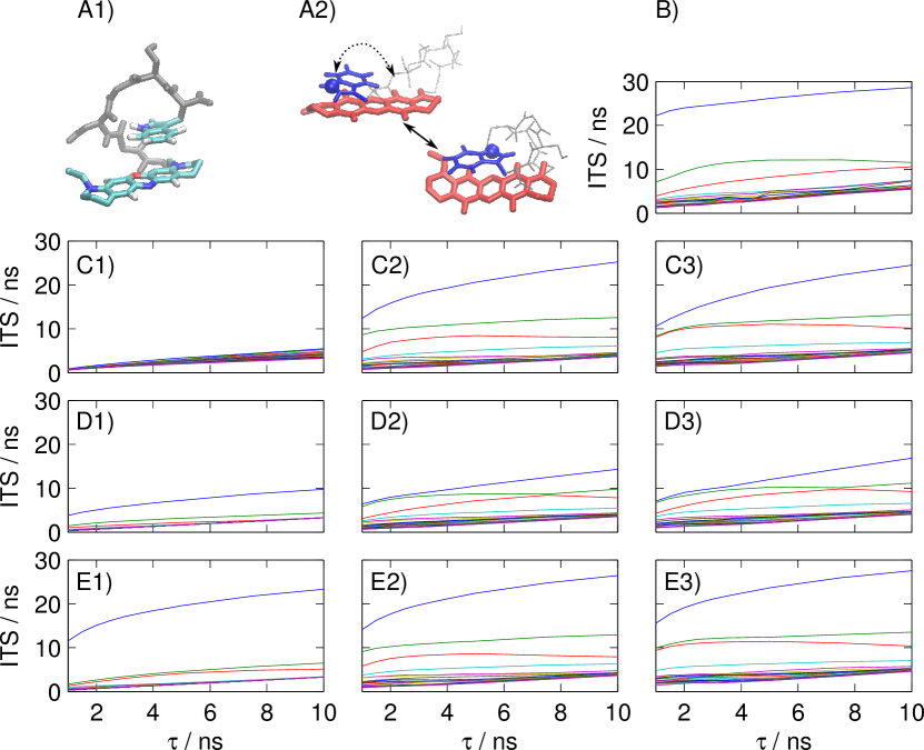
Fig. 2A1 shows a sample structure of MR121-GSGSW. Fig 2B shows a benchmark for the relaxation timescales computed by a regular-space clustering in pairwise minimal RMSD metric using 1000 cluster centers. The slowest processes are found at about 25 ns, 12 ns and 8 ns, slightly larger—and thus more accurate according to the variational principle in Eq. (4)—than by the coarser Markov model in [65]. To set up the direct clustering, two internal coordinate sets are considered: (i) the set of 66 distances between 12 coordinates defined by the 5 ’s and the 7 ring centers involved, and (ii) the center position and the orientation vector coordinates of the tryptophan sidechain in a coordinate set defined by the MR121 principal axes (see Fig. 2A2 for an illustration). Fig. 2c1-3 show the results of direct k-means clustering with 1000 cluster centers in the space of 66 intramolecular distances (C1), only the 9 tryptophan coordinates (C2), and the combined set (C3). It is clearly seen that the intramolecular distances are not suited to resolve the slowest processes, while the tryptophan coordinates resolve them very well. This can be understood from the structural arrangements shown in Fig. 3 that are dominated by the relative orientation of the tryptophan sidechain with respect to the MR121 ring system. Especially the slowest process, the stacking-order exchange of the two ring systems, cannot be well described by the intramolecular distances that are similar when the tryptophan is “above” or “below” the MR121. Fig. 2C3 shows that discretizing the combined coordinate set resolves the slowest processes with similar timescales as in the 9 Trp-coordinate set alone. This is not always expected, as increasing the dimensionality of the space to be clustered while keeping the number of clusters constant will often reduce the resolution.
In the subsequent PCA and TICA analysis different linear subspaces of the combined coordinate set were considered. Interestingly, clustering the principal components reduces the quality of the Markov model significantly. This is explained by the fact that the largest-amplitude motions in the present system is the transition between structures in which Trp and MR121 are in contact, and open structures. However, open structures have a very low population, giving rise to a rather fast timescale of the opening/closing process. The slowest processes, involving different arrangements and orientations of the Trp and MR121 while being in contact, give rise to comparatively small amplitude motions. Using one and four PCA components (D1 and D2), the three slowest processes are not found. Using ten PCA components, the two slowest processes are found, although slightly underestimated, while the third-slowest process is not found.
Fig. 2E1-3 shows that the TICA coordinates perform indeed very well. Using only the single slowest TICA coordinate does resolve the slowest process well and gives rise to a timescale of 20-25 ns, close to the expected value. Using the four slowest TICA coordinates resolves the two slowest processes well, while somewhat underestimating the third process. With ten TICA coordinates all slow processes are well resolved, and the timescales are found to be 27 ns, 13 ns, and 10 ns at a lagtime of 10 ns—slightly larger than in any of the other choices of metrics.
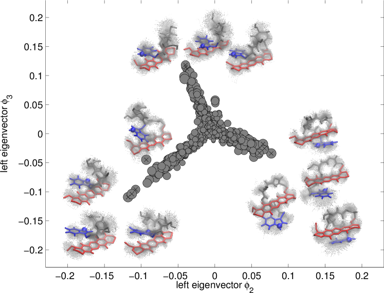
Fig. 3A illustrates the structural transition involved in the two slowest processes occurring at around 27 and 13 ns computed from the ten-dimensional TICA Markov model. We display the 1000 microstates in a visualization that we shall call kinetic map, where the coordinates are given by the two slowest left eigenvectors , . For example, a cluster is drawn at a position with a size proportional to its stationary probability . The map is termed “kinetic”, because similar positions in eigenvector spaces mean that the states can relatively quickly reach one another, while distant positions only exchange on timescales on the horizontal, and on timescale on the vertical axis. The left eigenvectors are chosen instead of the right eigenvectors, because the left eigenvectors are weighted by the stationary distribution: . Thus, points on the border of the map tend to have larger stationary probability. Therefore, the extremal points are at the same time populous and kinetically distant, and can roughly be associated with the most stable “free energy minima”, while the smaller clusters connecting them correspond to transition states. The structures, shown for the most populous and kinetically distinct clusters, indicate that the slowest relaxations are associated with a stacking-order exchange of the MR121 and Trp groups, and a rotation of the Trp group with respect to the MR121 group (see “marker” atom shown as a blue sphere).
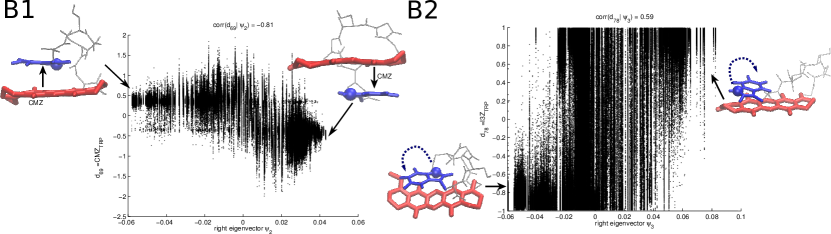
Fig. 3B illustrates the optimal indicators of the slowest processes, i.e. the input order parameters that have the largest correlation with the individual right Markov model eigenvectors and . The correlation plots show that the respective order parameters attain clearly different values at the end-states of the transition, i.e. for the minimal and maximal values of the respective eigenvector. At intermediate values of the eigenvectors, i.e. transition states, the order parameter can access many different values. This is easily seen in the slowest process (Fig. 3b1), where the best indicator is the Trp -position that mediates the stacking order exchange (correlation coefficient 0.84 with the second eigenvector ). While the value of the Trp -position is clearly defined in the transition end-states, where the Trp is located “above” and “below” the MR121 moiety, the transition states include open configurations where the Trp and the MR121 are not in contact at all, and therefore all values of the -position are accessible in these states. A similar behavior is seen for the second-slowest process (Trp sidechain rotation).
We now turn to another molecular system. Here, an extensive set of simulations of the kinase inducible domain (KID) in explicit solvent were investigated. KID is part of the cAMP response element-binding protein (CREB). CREB is a transcription factor involved in processes as important as glucose regulation and memory, and it binds the CREB-binding protein (CBP), a well-known cancer-related molecular hub with around 300 interacting protein partners [41]. KID belongs to a large and important class of intrinsically unstructured peptides (IUP), encompassing many hormones, domains and even whole proteins [91]. Unstructured regions perform their function even though they lack a well-defined secondary or tertiary structure in solution. Although standardized algorithms exist to detect unstructured regions on the basis of the primary amino acid sequence, the structural details of how disordered regions exert their function is still elusive. For example, some unstructured domains, including KID, become folded upon binding [89]; it is therefore of much interest (e.g. for the druggability of protein-protein interactions) to investigate whether the presence of pre-formed elements causes folded conformations to be selected from the ensemble (conformational selection) [54], or whether the binding rather occurs through induced-fit mechanics [85].
To shed light on this problem, we set-up an ensemble of all-atom simulations of the phosphorylated KID (pKID) domain. We have performed 7706 all-atom explicit-solvent simulations of 24 ns each using the ACEMD software [29] on the GPUGRID distributed computing platform [12], yielding a total 168 simulation data. However, due to the short simulations, only short lagtimes could be used, presenting a challenge to the Markov model construction. The detailed simulation setup is described in the Appendix.
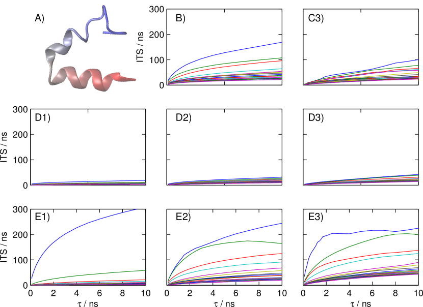
Fig. 4 shows the performance of different metrics in their ability to resolve the slowest processes of KID. KID is a more difficult case than the MR121-GSGSW peptide because its natively unstructured nature gives rise to many fast large-amplitude motions which will conceal the slow processes in most ad hoc metrics. Fig. 4B and C show that neither regular-space clustering in minimal pairwise RMSD metric, nor direct clustering in all distances yield a converged estimated of the timescales up to lagtimes of 10 ns. Between these two, regular-space RMSD is better, reaching a timescale of about 170 ns at , while the direct clustering produces a timescale below 100 ns at . Higher choices of lagtimes were avoided as they lead to a severe reduction of the usable data because the connected set of clusters drops significantly below 100% after that point. Fig. 4D1-3 show that the performance of principal components is even worse than direct clustering, giving rise to timescale estimates below 20 ns for one principal component and below 50 ns for ten principal components. This confirms that the largest-amplitude motions are not the slowest in KID.
Fig. 4E1-3 show the performance of the TICA coordinate using one, four, and ten dimensions. Using only the slowest TICA coordinate, a slow process of >200 ns is found, that has not been resolved by the clustering in any of the other metrics, however this timescale does not converge for lagtimes up to 10 ns. Using only the four slowest TICA coordinates, there are already three processes resolved that are above 100 ns, and the convergence behavior improves. Using the ten slowest TICA coordinates, five processes slower than 100 ns are resolved. The slowest process converges to a timescale around 220 ns and does so already at a lagtime of 2-5 ns. Thus, the lagtime needed is a factor of 50-100 smaller than the timescale of the process, indicating a very good discretization of the corresponding process.
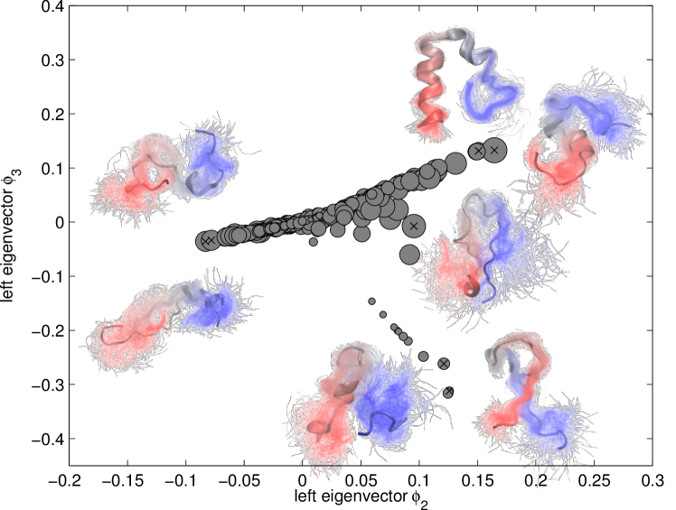
Fig. 5A illustrates the structural transitions associated with the two slowest relaxation processes of KID as identified by the Markov model using ten-dimensional TICA model. We have decided to focus on the two slowest processes around 200 and 220 ns relaxation time, because they are somewhat separated from the next-slowest processes occurring at around 100 ns. As the peptide has great structural variability it is of little value to plot all relevant structures. Therefore, we have plotted the positions of the microstates again in a kinetic map, using the coordinates of the two dominant left eigenvectors , . It is seen that at the slowest timescales, the system rearranges between mostly open and disordered structures (left), structures with one helix folded or partially folded (top right), and hairpin-like structures (bottom right). Thus the system has some residual helical structure, although it is not very stable in absence of a stabilizing binding partner.
Fig. 5B illustrates the optimal indicators of the slowest processes, i.e. the input order parameters that have the largest correlation with the resulting right Markov model eigenvectors and . Like for MR121-GSGSW, the correlation plots show that the respective order parameters are mainly able to distinguish the end-states of the transition, but unlike for MR121-GSGSW, multiple distances are almost equally good indicators for the same process. Fig. 5B shows correlation plots of the best indicators of and , but indicates the five best correlations (all correlation coefficients above 0.7) in the structure. It is seen that the slowest process (timescale 220 ns) is best described by a hinge opening and closing, where the closed hinge appears to induce at least partial formation of the N-terminal helix (red, see Fig. 5B2). This is consistent with NMR experiments that have shown the N-terminal region to be approximately 50% helical in the apo-form [73]. The second-slowest process (timescale 200 ns) is best described by partial helix formation of the C-terminal part (blue) of the protein.
5 Discussion
In the present manuscript we have derived a method to find the optimal linear combination of input coordinates for approximating the slowest relaxation processes in complex conformational rearrangements of molecules. It is shown that an implementation for this method is already known in statistics as the TICA method, which is combined here with Markov modeling in order to construct models of the slow relaxation processes and precise estimates of the related relaxation timescales. It is shown that this approach of constructing Markov models yields slower timescales, and thus a more precise approximation to the true relaxation processes, than previous approaches. This is also achieved for the natively unstructured peptide KID where established approaches such as direct clustering in distance space, minimal-RMSD-based clustering, or clustering in PCA space did not perform well because the largest-amplitude motions were not good indicators of the slowest relaxation processes.
Beyond having an approach to construct quantitatively accurate Markov models in a way that is more robust than most previous approaches, we readily obtain a way to find best indicators of the slowest transitions. Best indicators are those molecular order parameters that are best correlated with the Markov model Eigenvectors describing the slowest processes, and thus serve as candidates for good reaction coordinates. Being able to point out such indicators provides a way to make the sometimes complex structural rearrangements readily understandable.
Acknowledgements
We thank all the volunteers of GPUGRID who donated GPU computing time to the project. We are grateful to Thomas Weikl (MPI Potsdam) for advice and support. G.P.-H. acknowledges support from German Science Foundation DFG fund NO 825-3. F.P. acknowledges funding from the Max Planck society. T.G. gratefully acknowledges former support from the “Beatriu de Pinós” scheme of the Agència de Gestió d’Ajuts Universitaris i de Recerca (Generalitat de Catalunya). G.D.F. acknowledges support from the Ramón y Cajal scheme and support by the Spanish Ministry of Science and Innovation (Ref. BIO2011-27450). F.N. acknowledges funding from DFG center Matheon.
A
A
Appendix
Derivation of TICA
The generalized Eigenvalue problem of Eq. (9), and more specifically the TICA problem can be derived in different ways. It goes back to the classical Ritz method [75] and can be found in many mathematical texts. In the following we sketch a standard derivation using variational calculus, see also [36, 2] for a thorough discussion of this approach.
Let be a vector of coordinates used, for example distances or Cartesian positions. Without restriction of generality we assume that is mean-free, i.e. the mean of the data has already been subtracted. Note that is contains generally only a subset of the full phase space coordinates, thus is a subset of .
We now seek new coordinates as a linear transformation of such that
-
1.
are uncorrelated
-
2.
the autocovariances of at a fixed lag time are maximal.
We will show that if coordinates are given by a weighted sum of
| (18) |
the weight coefficients have to fulfill the generalized eigenvalue problem (see theory section)
| (19) |
where is the time-lagged covariance matrix that is defined by:
| (20) |
To prove this we rewrite the covariance matrix of and the time-lagged covariance matrix of using the defining equations (18), and (20).
We wish to maximize (property 3) under the constraint, that (property 2). We start by computing one coordinate with maximal autocovariance. It is given by the weighted sum , where we used the shorthand notation . The constraint (2) for is now .
Since the matrix-elements are fixed, the autocovariance can be treated as a differentiable function of the coefficients . Therefore, we need to maximize the function
where is the Lagrange multiplier. We perform the maximization by setting the partial derivatives of with respect to the weight coefficients to zero.
Rearranging and rewriting this equation in matrix-vector form leads to (19) for . The same argument is used for the subsequent eigenvalues. We now prove that the solutions of (19) fulfill the properties requested above:
-
1.
The IC’s obtained by solving (19) are uncorrelated: Let be a generalized eigenvector with eigenvalue and let be a generalized eigenvector with eigenvalue . Then the orthogonality condition
(21) will hold if and are symmetric matrices. If and are used as the weights in (18) this is equivalent to .
Proof:Therefore . Because the orthogonality condition must hold. This does not hold, if eigenvectors are degenerate i.e. for some , . However degeneracy can be avoided by changing the lag time such that no eigenvalues with large magnitude coincide. Solutions with smaller eigenvalues might still be degenerate, but this is unproblematic since these solutions are discarded for clustering. In addition, “fast” modes will necessarily be uncorrelated with “slow” modes, because their eigenvalues are far apart.
-
2.
The autocovariances at a fixed lag time are maximal:
We show that the autocovariances are identical to the Lagrange multipliers, and thus to the eigenvalues in Eq. 19:(22) To see this, multiply (19) with from the left, to obtain
now use the orthogonality condition (21)
To show that the optimum found is indeed a maximum, we calculate the Hessian of the constrained autocovariance . Its elements are:
and show that it is a positive definite matrix
We first expand in the basis of the generalized eigenvectors and use equations (21) and (22)
Without loss of generality, we assume that the solution vectors of Eq. (19) were sorted by descending eigenvalues to obtain an ordering from “slow” modes to “fast” modes, . From this follows for the first solution . The second solution is restricted to a subspace that is orthogonal to according to (21) and (22)
Therefore we can ignore the coefficient in the development of and obtain the quadratic form
Again, this is negative, because is the largest eigenvalue in the sum. This procedure can be extended to the third, fourth,… eigenvalue, showing that the optima are minima for all solutions.
As a result, we can sort the solution vectors of Eq. (19) by descending eigenvalues to obtain an ordering from “slow” modes to “fast” modes.
Symmetricity and Symmetrization of the time-lagged covariance matrix
Consider the correlation matrix of mean-free coordinates for lag time :
and the correlation matrix for lag time :
where is the unconditional transition probability between the set and the set within time lag . In statistically reversible dynamics, such an unconditional set-transition probability is symmetric (this follows directly from integrating the detailed balance condition over the sets). Thus, we can exchange time indexes and show:
And then trivially
When estimating correlation or covariance matrices from simulations, one cannot expect to hold. A trivial method is to use
where is the simulation estimate.
Simulation setup, KID
The coordinates of the phosphorylated KID domain (28 residues, CREB residues 119-146) were extracted from chain B of the entry 1KDX deposited in the Protein Data Bank. The entry represent the folded configuration of the pKID-CBP bound structure, determined through NMR [89]. Neutral acetylated and N-methyl caps were added to avoid artifactual charges at the peptide’s termini; the protein was solvated with 6572 water molecules and a 85 mM KCl concentration (matching the experimental ionic strength). The system was then parametrized with the AMBER ff99SB-ILDN forcefield [49]; water and ions were modeled respectively with the TIP3P and Joung-Cheatham parameter sets [38, 37]. The system thus prepared was first equilibrated for 24 ns in the constant-pressure ensemble, during which it stabilized at a volume of approximately 60 Å3. The peptide was then denatured by heating it at 500 ºK for 17.6 ns in constant-volume conditions; 176 frames were extracted from this trajectory and used as starting configurations for the production runs. All of the simulations were performed with a time step of 4 fs, enabled by the hydrogen mass repartitioning scheme [25]; long-range electrostatic forces were computed with the particle-mesh Ewald summation method. A nonbonded cutoff distance of 9 Å was used with a switching distance of 7.5 Å for Van der Waals interactions, while the lengths of bonds involving hydrogen atoms were constrained with the SHAKE algorithm.
A set of 7706 production runs was executed on the GPUGRID distributed computing network [12]. Each simulation was performed in the constant-volume ensemble at 315 ºK for 24 ns with the same parametrization used for equilibration, storing structural snapshots every 100 ps. Each production simulation begun either from one of the configurations visited during the denaturation run, or frames visited during preceding production trajectories. Starting frames were selected iteratively with an adaptive strategy in order to minimize the statistical uncertainty on the largest eigenvalue, computed on the already available simulation data, based on Singhal and Pande’s algorithm [31].
References
- [1] Aapo Hyvärinen, Juha Karhunen, and Erkki Oja. Independent Component Analysis, chapter 18, page 344. John Wiley & Sons, 2001.
- [2] Erkki Oja Aapo Hyvärinen, Juha Karhunen. Independent Component Analysis. John Wiley & Sons, 2001.
- [3] Alexandros Altis, Moritz Otten, Phuong H. Nguyen, Rainer Hegger, and Gerhard Stock. Construction of the free energy landscape of biomolecules via dihedral angle principal component analysis. The Journal of Chemical Physics, 128(24):245102, 2008.
- [4] A. Amadei, A. B. Linssen, and H. J. C. Berendsen. Essential dynamics of proteins. Proteins, 17:412–225, 1993.
- [5] Kyle A. Beauchamp, Gregory R. Bowman, Thomas J. Lane, Lutz Maibaum, Imran S. Haque, and Vijay S. Pande. MSMBuilder2: Modeling Conformational Dynamics at the Picosecond to Millisecond Scale. Journal of chemical theory and computation, 7(10):3412–3419, October 2011.
- [6] Kyle A. Beauchamp, Robert McGibbon, Yu-Shan Lin, and Vijay S. Pande. Simple few-state models reveal hidden complexity in protein folding. Proceedings of the National Academy of Sciences, 2012.
- [7] Alexander Berezhkovskii, Gerhard Hummer, and Attila Szabo. Reactive flux and folding pathways in network models of coarse-grained protein dynamics. The Journal of chemical physics, 130(20), May 2009.
- [8] Xevi Biarnés, Fabio Pietrucci, Fabrizio Marinelli, and Alessandro Laio. Metagui. a vmd interface for analyzing metadynamics and molecular dynamics simulations. Computer Physics Communications, 183(1):203–211, Jan 2012.
- [9] Gregory R. Bowman, Kyle A. Beauchamp, George Boxer, and Vijay S. Pande. Progress and challenges in the automated construction of Markov state models for full protein systems. J. Chem. Phys., 131(12):124101+, September 2009.
- [10] Gregory R. Bowman and Phillip L. Geissler. Equilibrium fluctuations of a single folded protein reveal a multitude of potential cryptic allosteric sites. Proceedings of the National Academy of Sciences, 109(29):11681–11686, 2012.
- [11] Gregory R. Bowman, Vincent A. Voelz, and Vijay S. Pande. Atomistic Folding Simulations of the Five-Helix Bundle Protein Lambda 6-85. Journal of the American Chemical Society, 133(4):664–667, February 2011.
- [12] I. Buch, M. J. Harvey, T. Giorgino, D. P. Anderson, and G. De Fabritiis. High-throughput all-atom molecular dynamics simulations using distributed computing. Journal of Chemical Information and Modeling, 50(3):397–403, Mar 2010.
- [13] Ignasi Buch, Toni Giorgino, and Gianni De Fabritiis. Complete reconstruction of an enzyme-inhibitor binding process by molecular dynamics simulations. Proceedings of the National Academy of Sciences, 108(25):10184–10189, June 2011.
- [14] Nicaolae V. Buchete and Gerhard Hummer. Coarse Master Equations for Peptide Folding Dynamics. J. Phys. Chem. B, 112:6057–6069, 2008.
- [15] Ginka S. Buchner, Ronan D. Murphy, Nicolae-Viorel Buchete, and Jan Kubelka. Dynamics of protein folding: Probing the kinetic network of folding–unfolding transitions with experiment and theory. Biochimica et Biophysica Acta, 1814:1001–1020, 2011.
- [16] J. D. Chodera, K. A. Dill, N. Singhal, V. S. Pande, W. C. Swope, and J. W. Pitera. Automatic discovery of metastable states for the construction of Markov models of macromolecular conformational dynamics. J. Chem. Phys., 126:155101, 2007.
- [17] H.S. Chung, J.M. Louis, and W.A. Eaton. Single-molecule fluorescence experiments determine protein folding transition path times. Science, 335:981–984, 2012.
- [18] R. R. Coifman, S. Lafon, A. B. Lee, M. Maggioni, B. Nadler, F. Warner, and S. W. Zucker. Geometric diffusions as a tool for harmonic analysis and structure definition of data: Diffusion maps. Proc. Natl. Acad. Sci. USA, 102:7426–7431, 2005.
- [19] Isabella Daidone, Hannes Neuweiler, Sören Doose, Markus Sauer, and Jeremy C. Smith. Hydrogen-bond driven loop-closure kinetics in unfolded polypeptide chains. PloS One, 6:e1000645+, 2010.
- [20] S. Dasgupta and P. Long. Performance guarantees for hierarchical clustering. J. Comput. Syst. Sci., 70(4):555–569, June 2005.
- [21] B. de Groot, X. Daura, A. Mark, and H. Grubmüller. Essential Dynamics of Reversible Peptide Folding: Memory-free Conformational Dynamics Governed by Internal Hydrogen Bonds. J. Mol. Bio., 301:299–313, 2001.
- [22] P. Deuflhard and M. Weber. Robust Perron cluster analysis in conformation dynamics. ZIB Report, 03-09, 2003.
- [23] Natasa Djurdjevac, Marco Sarich, and Christof Schütte. Estimating the eigenvalue error of Markov State Models. Multiscale Model. Simul., 10:61–81, 2012.
- [24] Elan Z. Eisenmesser, Oscar Millet, Wladimir Labeikovsky, Dmitry M. Korzhnev, Magnus Wolf-Watz, Daryl A. Bosco, Jack J. Skalicky, Lewis E. Kay, and Dorothee Kern. Intrinsic dynamics of an enzyme underlies catalysis. Nature, 438(7064):117–121, November 2005.
- [25] K. Anton Feenstra, Berk Hess, and Herman J. C. Berendsen. Improving efficiency of large time-scale molecular dynamics simulations of hydrogen-rich systems. Journal of Computational Chemistry, 20(8):786–798, 1999.
- [26] S. Fischer, B. Windshuegel, D. Horak, K. C. Holmes, and J. C. Smith. Structural mechanism of the recovery stroke in the Myosin molecular motor. Proc. Natl. Acad. Sci. USA, 102:6873–6878, 2005.
- [27] Alexander Gansen, Alessandro Valeri, Florian Hauger, Suren Felekyan, Stanislav Kalinin, Katalin Tóth, Jörg Langowski, and Claus A. M. Seidel. Nucleosome disassembly intermediates characterized by single-molecule FRET. Proc. Natl. Acad. Sci. USA, 106(36):15308–15313, September 2009.
- [28] Gebhardt, Thomas Bornschlögl, and Matthias Rief. Full distance-resolved folding energy landscape of one single protein molecule. Proc. Natl. Acad. Sci. USA, 107(5):2013–2018, February 2010.
- [29] M. J. Harvey, G. Giupponi, and G. De Fabritiis. Acemd: Accelerating biomolecular dynamics in the microsecond time scale. Journal of Chemical Theory and Computation, 5(6):1632–1639, Jun 2009.
- [30] Martin Held, Philipp Metzner, and Frank Noé. Mechanisms of protein-ligand association and its modulation by protein mutations. Biophys. J., 100:701–710, 2011.
- [31] Nina Singhal Hinrichs and Vijay S. Pande. Calculation of the distribution of eigenvalues and eigenvectors in markovian state models for molecular dynamics. The Journal of Chemical Physics, 126(24):244101–244101–11, Jun 2007.
- [32] Danzhi Huang and Amedeo Caflisch. The Free Energy Landscape of Small Molecule Unbinding. PLoS Comput Biol, 7(2):e1002002+, February 2011.
- [33] Isaac A. Hubner, Eric J. Deeds, and Eugene I. Shakhnovich. Understanding ensemble protein folding at atomic detail. Proc. Natl. Acad. Sci. USA, 103(47):17747–17752, November 2006.
- [34] M. Jäger, Y. Zhang, J. Bieschke, H. Nguyen, M. Dendle, M. E. Bowman, J. P. Noel, M. Gruebele, and J. W. Kelly. Structure-function-folding relationship in a WW domain. Proc. Natl. Acad. Sci. USA, 103:10648–10653, 2006.
- [35] Abhinav Jain, Rainer Hegger, and Gerhard Stock. Hidden complexity of protein free-energy landscapes revealed by principal component analysis by parts. The Journal of Physical Chemistry Letters, 1(19):2769–2773, 2010.
- [36] I.T. Jolliffe. Principal Component Analysis. Springer, New York, 2 edition, 2002.
- [37] William L. Jorgensen, Jayaraman Chandrasekhar, Jeffry D. Madura, Roger W. Impey, and Michael L. Klein. Comparison of simple potential functions for simulating liquid water. The Journal of Chemical Physics, 79(2):926–935, July 1983.
- [38] In Suk Joung and Thomas E. Cheatham. Determination of alkali and halide monovalent ion parameters for use in explicitly solvated biomolecular simulations. The Journal of Physical Chemistry. B, 112(30):9020–9041, Jul 2008. PMID: 18593145 PMCID: 2652252.
- [39] W. Kabsch. A solution for the best rotation to relate two sets of vectors. Acta Crystallographica Section A, 32(5):922–923, Sep 1976.
- [40] Mary E. Karpen, Douglas J. Tobias, and Charles L. Brooks. Statistical clustering techniques for the analysis of long molecular dynamics trajectories: analysis of 2.2-ns trajectories of YPGDV. Biochemistry, 32(2):412–420, January 1993.
- [41] Lawryn H Kasper, Tomofusa Fukuyama, Michelle A Biesen, Fayçal Boussouar, Caili Tong, Antoine de Pauw, Peter J Murray, Jan M A van Deursen, and Paul K Brindle. Conditional knockout mice reveal distinct functions for the global transcriptional coactivators CBP and p300 in T-cell development. Molecular and cellular biology, 26(3):789–809, Feb 2006. PMID: 16428436.
- [42] L. Kaufman and P.J. Rousseeuw. Statistical Data Analysis Based on the L_1-Norm and Related Methods, chapter Clustering by means of Medoids, pages 405–416. North-Holland, 1987.
- [43] Bettina Keller, Jan-Hendrik Prinz, and Frank Noé. Markov models and dynamical fingerprints: Unraveling the complexity of molecular kinetics. Chem. Phys., 396:92–107, 2012.
- [44] Andrei Y. Kobitski, Alexander Nierth, Mark Helm, Andres Jäschke, and G. Ulrich Nienhaus. Mg2+ dependent folding of a Diels-Alderase ribozyme probed by single-molecule FRET analysis. Nucleic Acids Res., 35:2047–2059, 2007.
- [45] S. V. Krivov and M. Karplus. Hidden complexity of free energy surfaces for peptide (protein) folding. Proc. Nat. Acad. Sci. USA, 101:14766–14770, 2004.
- [46] Susanna Kube and Marcus Weber. A coarse graining method for the identification of transition rates between molecular conformations. J. Chem. Phys., 126(2):024103+, 2007.
- [47] L. Tong, V.C. Soon, Y.F. Huang, and R. Liu. AMUSE: a new blind identification algorithm. Circuits and Systems, 3:1784–1787, 1990.
- [48] Kresten Lindorff-Larsen, Stefano Piana, Ron O. Dror, and David E. Shaw. How fast-folding proteins fold. Science, 334:517–520, 2011.
- [49] Kresten Lindorff-Larsen, Stefano Piana, Kim Palmo, Paul Maragakis, John L Klepeis, Ron O Dror, and David E Shaw. Improved side-chain torsion potentials for the Amber ff99SB protein force field. Proteins, 78(8):1950–1958, Jun 2010. PMID: 20408171 PMCID: PMC2970904.
- [50] S.P. Lloyd. Least squares quantization in pcm. IEEE Transactions on Information Theory, 28:129–137, 1982.
- [51] P. Metzner, C. Schütte, and E. Vanden Eijnden. Transition Path Theory for Markov Jump Processes. Multiscale Model. Simul., 7:1192–1219, 2009.
- [52] W. Min, G. Luo, B. J. Cherayil, S. C. Kou, and X. S. Xie. Observation of a Power-Law Memory Kernel for Fluctuations within a Single Protein Molecule. Phys. Rev. Lett., 94:198302+, 2005.
- [53] Ayori Mitsutake, Hiromitsu Iijima, and Hiroshi Takano. Relaxation mode analysis of a peptide system: Comparison with principal component analysis. The Journal of Chemical Physics, 135(16):164102, 2011.
- [54] Amrita Mohan, Christopher J. Oldfield, Predrag Radivojac, Vladimir Vacic, Marc S. Cortese, A. Keith Dunker, and Vladimir N. Uversky. Analysis of molecular recognition features (MoRFs). Journal of Molecular Biology, 362(5):1043–1059, Oct 2006.
- [55] L. Molgedey and H. G. Schuster. Separation of a mixture of independent signals using time delayed correlations. Phys. Rev. Lett., 72:3634–3637, Jun 1994.
- [56] Stefanie Muff and Amedeo Caflisch. Kinetic analysis of molecular dynamics simulations reveals changes in the denatured state and switch of folding pathways upon single-point mutation of a -sheet miniprotein. Proteins, 70:1185–1195, 2007.
- [57] Yusuke Naritomi and Sotaro Fuchigami. Slow dynamics in protein fluctuations revealed by time-structure based independent component analysis: The case of domain motions. The Journal of Chemical Physics, 134(6):065101, 2011.
- [58] Heike Neubauer, Natalia Gaiko, Sylvia Berger, Jörg Schaffer, Christian Eggeling, Jennifer Tuma, Laurent Verdier, Claus A. Seidel, Christian Griesinger, and Andreas Volkmer. Orientational and dynamical heterogeneity of rhodamine 6G terminally attached to a DNA helix revealed by NMR and single-molecule fluorescence spectroscopy. J. Am. Chem. Soc., 129(42):12746–12755, October 2007.
- [59] Hannes Neuweiler, Marc Löllmann, Sören Doose, and M. Sauer. Dynamics of Unfolded Polypeptide Chains in Crowded Environment Studied by Fluorescence Correlation Spectroscopy. J. Mol. Biol., 365:856–869, 2007.
- [60] F. Noé, I. Daidone, J. C. Smith, A. di Nola, and A. Amadei. Solvent Electrostriction Driven Peptide Folding revealed by Quasi-Gaussian Entropy Theory and Molecular Dynamics Simulation. Journal of Physical Chemistry B, 112:11155–11163, 2008.
- [61] F. Noé and S. Fischer. Transition networks for modeling the kinetics of conformational transitions in macromolecules. Curr. Opin. Struc. Biol., 18:154–162, 2008.
- [62] F. Noé, I. Horenko, C. Schütte, and J. C. Smith. Hierarchical Analysis of Conformational Dynamics in Biomolecules: Transition Networks of Metastable States. J. Chem. Phys., 126:155102, 2007.
- [63] F. Noé, D. Krachtus, J. C. Smith, and S. Fischer. Transition Networks for the Comprehensive Characterization of Complex Conformational Change in Proteins. J. Chem. Theo. Comp., 2:840–857, 2006.
- [64] Frank Noé. Probability Distributions of Molecular Observables computed from Markov Models. J. Chem. Phys., 128:244103, 2008.
- [65] Frank Noé, Sören Doose, Isabella Daidone, Marc Löllmann, John D. Chodera, Markus Sauer, and Jeremy C. Smith. Dynamical fingerprints for probing individual relaxation processes in biomolecular dynamics with simulations and kinetic experiments. Proc. Natl. Acad. Sci. USA, 108:4822–4827, 2011.
- [66] Frank Noé and Feliks Nüske. A variational approach to modeling slow processes in stochastic dynamical systems. Multiscale Model. Simul. (submitted, available at: http://publications.mi.fu-berlin.de/1109/), 2012.
- [67] Frank Noé, Christof Schütte, Eric Vanden-Eijnden, Lothar Reich, and Thomas R. Weikl. Constructing the full ensemble of folding pathways from short off-equilibrium simulations. Proc. Natl. Acad. Sci. USA, 106:19011–19016, 2009.
- [68] Andreas Ostermann, Robert Waschipky, Fritz G. Parak, and Ulrich G. Nienhaus. Ligand binding and conformational motions in myoglobin. Nature, 404:205–208, 2000.
- [69] Albert C. Pan and Benoît Roux. Building Markov state models along pathways to determine free energies and rates of transitions. J. Chem. Phys., 129(6):064107+, August 2008.
- [70] Menahem Pirchi, Guy Ziv, Inbal Riven, Sharona Sedghani Cohen, Nir Zohar, Yoav Barak, and Gilad Haran. Single-molecule fluorescence spectroscopy maps the folding landscape of a large protein. Nature Comms, 2:493, 2011.
- [71] Jan-Hendrik Prinz, John D. Chodera, and Frank Noé. Robust rate estimate from spectral estimation. Phys. Rev. Lett. (submitted), 2011.
- [72] Jan-Hendrik Prinz, Hao Wu, Marco Sarich, Bettina Keller, Martin Fischbach, Martin Held, John D. Chodera, Christof Schütte, and Frank Noé. Markov models of molecular kinetics: Generation and validation. J. Chem. Phys., 134:174105, 2011.
- [73] Ishwar Radhakrishnan, Gabriela C Pérez-Alvarado, David Parker, H.Jane Dyson, Marc R Montminy, and Peter E Wright. Solution structure of the kix domain of cbp bound to the transactivation domain of creb: A model for activator:coactivator interactions. Cell, 91:741–752, 1997.
- [74] F. Rao and A. Caflisch. The Protein Folding Network. J. Mol. Bio., 342:299–306, 2004.
- [75] Walter Ritz. Über eine neue methode zur lösung gewisser variationsprobleme der mathematischen physik. Journal für die Reine und Angewandte Mathematik, 135:1–61, 1909.
- [76] M. A. Rohrdanz, W. Zheng, M. Maggioni, and C. Clementi. Determination of reaction coordinates via locally scaled diffusion map. J. Chem. Phys., 134(124116), 2011.
- [77] S. K. Sadiq, F. Noé, and G. de Fabritiis. Kinetic characterization of the critical step in hiv-1 protease maturation. Proc. Natl. Acad. Sci. USA (in press), 2012.
- [78] Yusdi Santoso, Catherine M. Joyce, Olga Potapova, Ludovic Le Reste, Johannes Hohlbein, Joseph P. Torella, Nigel D. F. Grindley, and Achillefs N. Kapanidis. Conformational transitions in DNA polymerase I revealed by single-molecule FRET. Proc. Natl. Acad. Sci. USA, 107(2):715–720, January 2010.
- [79] Marco Sarich, Frank Noé, and Christof Schütte. On the approximation error of markov state models. SIAM Multiscale Model. Simul., 8:1154–1177, 2010.
- [80] V. Schultheis, T. Hirschberger, H. Carstens, and P. Tavan. Extracting Markov Models of Peptide Conformational Dynamics from Simulation Data. J. Chem. Theory Comp., 1:515–526, 2005.
- [81] C. Schütte, A. Fischer, W. Huisinga, and P. Deuflhard. A Direct Approach to Conformational Dynamics based on Hybrid Monte Carlo. J. Comput. Phys., 151:146–168, 1999.
- [82] M. Seeber, A. Felline, F. Raimondi, S. Muff, Ran Friedman, F. Rao, A. Caflisch, and F. Fanelli. Wordom: a user-friendly program for the analysis of molecular structures, trajectories, and free energy surfaces. J. Comp. Chem., 6:1183–1194, 2011.
- [83] M. Senne, B. Trendelkamp-Schroer, A.S.J.S. Mey, C. Schütte, and F. Noé. Emma - a software package for markov model building and analysis. J. Chem. Theory and Comput., 8:2223–2238, 2012.
- [84] David E. Shaw, Paul Maragakis, Kresten Lindorff-Larsen, Stefano Piana, Ron O. Dror, Michael P. Eastwood, Joseph A. Bank, John M. Jumper, John K. Salmon, Yibing Shan, and Willy Wriggers. Atomic-Level Characterization of the Structural Dynamics of Proteins. Science, 330(6002):341–346, October 2010.
- [85] Benjamin A. Shoemaker, John J. Portman, and Peter G. Wolynes. Speeding molecular recognition by using the folding funnel: The fly-casting mechanism. Proceedings of the National Academy of Sciences, 97(16):8868–8873, Aug 2000.
- [86] N. Singhal and V. S. Pande. Error analysis and efficient sampling in Markovian state models for molecular dynamics. J. Chem. Phys., 123:204909, 2005.
- [87] S. Sriraman, I. G. Kevrekidis, and G. Hummer. Coarse Master Equation from Bayesian Analysis of Replica Molecular Dynamics Simulations. J. Phys. Chem. B, 109:6479–6484, 2005.
- [88] Johannes Stigler, Fabian Ziegler, Anja Gieseke, J. Christof M. Gebhardt, and Matthias Rief. The complex folding network of single calmodulin molecules. Science, 334:512–516, 2011.
- [89] Kenji Sugase, H. Jane Dyson, and Peter E. Wright. Mechanism of coupled folding and binding of an intrinsically disordered protein. Nature, 447(7147):1021–1025, Jul 2007.
- [90] W. C. Swope, J. W. Pitera, and F. Suits. Describing protein folding kinetics by molecular dynamics simulations: 1. Theory. J. Phys. Chem. B, 108:6571–6581, 2004.
- [91] Vladimir N. Uversky. Intrinsically disordered proteins from A to Z. The International Journal of Biochemistry & Cell Biology, 43(8):1090–1103, Aug 2011.
- [92] Vincent A. Voelz, Gregory R. Bowman, Kyle Beauchamp, and Vijay S. Pande. Molecular Simulation of ab Initio Protein Folding for a Millisecond Folder NTL9. J. Am. Chem. Soc., 132(5):1526–1528, February 2010.
- [93] D. J. Wales. Energy Landscapes. Cambridge University Press, Cambridge, 2003.
- [94] M. Weber. Improved Perron cluster analysis. ZIB Report, 03-04, 2003.
- [95] Beth G. Wensley, Sarah Batey, Fleur A. C. Bone, Zheng M. Chan, Nuala R. Tumelty, Annette Steward, Lee G. Kwa, Alessandro Borgia, and Jane Clarke. Experimental evidence for a frustrated energy landscape in a three-helix-bundle protein family. Nature, 463(7281):685–688, February 2010.