The Distribution of Alpha Elements in Ultra-Faint Dwarf Galaxies

Abstract

The Milky Way ultra$-$faint dwarf galaxies (UFDs) contain some of the oldest, most metal$-$poor stars in the Universe. We present [Mg/Fe], [Si/Fe], [Ca/Fe], [Ti/Fe], and mean $[\alpha/\rm{Fe}]$  abundance ratios for 61  individual red giant branch stars across 8  UFDs. This is the largest sample of alpha abundances published to date in galaxies with absolute magnitudes M_V $>$ $-$8, including the first measurements for Segue 1, Canes Venatici II, Ursa Major I, and Leo T. Abundances were determined via medium$-$resolution Keck/DEIMOS spectroscopy and spectral synthesis. The sample spans the metallicity range $-$3.4  $<\rm{[Fe/H]}<$ $-$1.1. With the possible exception of Segue 1 and Ursa Major II, the individual UFDs show on average lower $[\alpha/\rm{Fe}]$  at higher metallicities, consistent with enrichment from Type Ia supernovae. Thus even the faintest galaxies have undergone at least a limited level of chemical self$-$enrichment. Together with recent photometric studies, this suggests that star formation in the UFDs was not a single burst, but instead lasted at least as much as the minimum time delay of the onset of Type Ia supernovae ($\sim 100$ Myr) and less than $\sim{2}$ Gyr. We further show that the combined population of UFDs has an $[\alpha/\rm{Fe}]$  abundance pattern that is inconsistent with a flat, Galactic halo$-$like alpha abundance trend, and is also qualitatively different from that of the more luminous CVn I dSph, which does show a hint of a plateau at very low [Fe/H].

1. Introduction

Ultra-faint dwarf (UFD) galaxies are the least luminous (M${}_{V}>-8$) known galaxies in the Universe (Willman et al. 2005b, a; Belokurov et al. 2006, 2007; Zucker et al. 2006a, b; Sakamoto & Hasegawa 2006, Walsh et al. 2007; Irwin et al. 2007). Spectroscopic observations of individual stars demonstrate that UFD galaxies are dark matter dominated (Simon & Geha, 2007). They obey the metallicity$-$luminosity relation found in the brighter, classical spheroidals (dSphs), and have large internal metallicity spreads greater than 0.5 dex (Kirby et al., 2008b).

Recent HST photometry extending below the main sequence turn$-$off demonstrates that at least three UFDs (Hercules, Ursa Major I and Leo IV) are composed exclusively of ancient stars $\sim{13}$ Gyr old (Brown et al., 2012). These data further suggest that the star formation lasted for less than $\sim{2}$ Gyr. In spite of this small age spread, the large metallicity spread in UFDs is indicative of a complex formation history. Metallicity spreads can arise in different ways. Star formation in a UFD may proceed continuously or in bursts within a single halo, on average increasing its metallicity over time (e.g., Lanfranchi & Matteucci, 2004; Revaz et al., 2009). Inhomogeneous gas mixing can also lead to a wide range of stellar metallicities within a single satellite (e.g., Argast et al., 2000; Oey, 2000). Finally, the merger of multiple progenitors with different mean metallicities may also produce a wide metallicity spread, as seen in recent simulations of more massive satellites (Wise et al., 2012). Determining more detailed abundances of stars in the UFDs will provide insight into the history of star formation at these very early epochs.

The $[\alpha/\rm{Fe}]$  abundance ratios, including [Mg/Fe], [Si/Fe], [Ca/Fe], and [Ti/Fe], provide important constraints on the chemical evolution history of a stellar population. In the most metal$-$poor stars, the ISM is polluted by the products of massive stellar evolution and core-collapse Type II supernovae (SNe). The chemical yields from these explosions (Woosley & Weaver 1995; Nomoto et al. 2006) result in super$-$solar $[\alpha/\rm{Fe}]$  values. These yields may depend on the mass, metallicity, and explosion energy of the supernova. Hence, individual Type II SNe may leave a unique signature in the observed abundance patterns, provided that (a) the gas did not have sufficient time to mix prior to the formation of the next generation of stars, or (b) the number of SNe was small, leading to stochastic sampling of the IMF. This would lead to intrinsic scatter in the [$\alpha$/Fe] ratios and/or abnormal abundance ratios. Given their low average metallicities, the UFDs are one of the best places to search for the signature of chemical enrichment from metal$-$free Population III stars (Frebel & Bromm, 2012).

Type Ia SNe output negligible amounts of alpha$-$elements in contrast to iron$-$peak elements resulting in lower $[\alpha/\rm{Fe}]$  with rising [Fe/H]. Due to the time delay in the onset of Type Ia SNe, the low $[\alpha/\rm{Fe}]$  signature is indicative of star formation lasting longer than the minimum time delay, $t_{\rm{min,Ia}}\sim 100$ Myr (Totani et al., 2008; Maoz et al., 2012). The [Fe/H] at which $[\alpha/\rm{Fe}]$  starts to decrease helps constrain the efficiency of star formation (Pagel 2009 and references therein). It thus provides a means to distinguish stellar populations with different origins. Spectroscopic studies of classical dSphs (e.g., Shetrone et al., 2001; Venn et al., 2004; Kirby et al., 2011) reported significantly lower $[\alpha/\rm{Fe}]$  in comparison to the observable Milky Way halo at [Fe/H] $\gtrsim{-2.5}$. This result has been used to show that the classical dSphs had a different chemical evolution than the progenitor(s) of the bulk of the inner Milky Way halo, which were likely more massive dwarf systems (Robertson et al., 2005). In contrast to the inner halo pattern, Nissen & Schuster (2010) have reported a population of nearby, low $[\alpha/\rm{Fe}]$  stars consistent with outer halo membership based on their kinematics, thus providing some indication that accreted systems with low $[\alpha/\rm{Fe}]$  abundance ratios were important contributors to the outer halo.

Our knowledge of the distribution of chemical abundances in UFDs, their chemical evolution, and their similarity/difference with the halo stars, is still limited. High-resolution (R $\gtrsim$ 20,000) abundance studies have begun to address these issues in the UFDs by targeting the brightest RGB stars for abundance analysis. These include studies of Ursa Major II and Coma Berenices (Frebel et al. 2010, 3 stars in each galaxy), Segue 1 (Norris et al. 2010a, 1 star), Leo IV (Simon et al. 2010, 1 star), Boötes I (Feltzing et al. 2009; 7 stars; Norris et al. 2010c, 1 star; Gilmore et al. 2013, 7 stars), and Hercules (Koch et al. 2008, 2 stars; Adén et al. 2011, 11 stars). These studies have primarily targeted the [Fe/H] $<-$2.0 regime. Adén et al. (2011) reported decreasing [Ca/Fe] with [Fe/H] in a sample of 9 stars in Hercules with [Fe/H] $<-2.0$. In contrast, Frebel et al. (2010) found similar $[\alpha/\rm{Fe}]$  abundance patterns at $\rm{[Fe/H]}<-2.5$ between the Coma Berenices and Ursa Major II UFDs, and the (flat) $[\alpha/\rm{Fe}]$$-$[Fe/H] pattern in the inner Milky Way halo. Thus, the role of the UFDs in building even the most metal$-$poor end of the inner halo is still unclear.

High$-$resolution abundance studies of UFDs are currently limited to relatively bright stars with apparent magnitude $V\lesssim{19}$. Coupled with the sparseness of the RGBs in UFD systems, high$-$resolution abundance studies using 8$-$10 meter class telescopes remain impractical for large samples. For example, the faintest star in a UFD studied to date at high$-$resolution is the brightest known RGB star in Leo IV with an apparent magnitude of $V\sim{19.2}$ (Simon et al., 2010). In order to build statistically meaningful samples of abundance measurements, we turned to medium-resolution spectroscopy.

Medium$-$resolution studies (R $\sim$ 2,000 $-$10,000) have recently begun to play a major role in obtaining precise abundances for larger stellar samples in both classical dSphs and UFDs. While lower spectral resolution reduces the number of chemical species available for study, medium$-$resolution spectroscopy has been used to successfully measure both iron (Allende Prieto et al., 2006; Lee et al., 2008; Kirby et al., 2008a) and alpha$-$element abundances (Kirby et al., 2009; Lee et al., 2011). Kirby et al. (2010) presented homogeneous Keck/DEIMOS medium$-$resolution abundances for thousands of stars in eight of the classical dSphs, showing that these systems may share a common trend of rising [$\alpha$/Fe] with decreasing [Fe/H] down to [Fe/H] $\sim{-2.5}$. Lai et al. (2011) reported halo$-$like [$\alpha$/Fe] ratios in Böotes I spanning $-3.8\lesssim{}\rm{[Fe/H]}\lesssim{-1.5}$, and Norris et al. (2010b) presented [C/Fe] for 16 stars in Böotes I and 3 stars in Segue 1, showing a wide range of carbon enhancements.

In this paper, we present the first homogeneous abundances for [Mg/Fe], [Si/Fe], [Ca/Fe], and [Ti/Fe] for 61  stars in 8  of the UFDs: Segue 1 (Seg 1), Coma Berenices (Com Ber), Ursa Major II (UMa II), Ursa Major I (UMa I), Canes Venatici II (CVn II), Leo IV, and Hercules (Herc). Our observations and abundance measurement technique are summarized in § 2$-$3. We present our abundance results in § 4$-$5 and discuss their implications in § 6.

2. Observations and Sample Selection

We determine spectroscopic abundances for the sample of UFD stars first presented by Simon & Geha (2007), hereafter SG07, Geha et al. (2009), and Simon et al. (2011), hereafter S11. The sample was observed with the Keck/DEIMOS spectrograph (Faber et al., 2003) using the 1200 line mm^-1 grating, which provided wavelength coverage between 6300 and 9100 Å  with a resolution of $\sim{1.3}$ Å  FWHM. Spectra were reduced using a modified version of the spec2d software pipeline (version 1.1.4) developed by the DEEP2 team (Newman et al., 2012; Cooper et al., 2012) optimized for stellar spectra (SG07). The final one-dimensional spectra include the random uncertainties per pixel. Radial velocities are measured by cross$-$correlating the science spectra with stellar templates, and are used in this work to shift the science spectra to the rest frame.

We analyze only stars identified as UFD members by SG07 and S11. These authors selected members on the basis of: (i) position in color$-$magnitude space relative to an M92 isochrone shifted to the UFD distance; (ii) radial velocity within $\sim{3}\sigma$ of the systemic UFD velocity; (iii) Na I $\lambda\lambda$8183,8195 equivalent width $\lesssim{1}$ Å, and (iv) a loose cut based on a Ca II infrared triplet (CaT) estimate of the stellar metallicity. The Na I criterion prevents contamination by disk dwarfs that share similar radial velocities and magnitudes as the UFD RGB stars. We refer the reader to SG07 for a detailed explanation of the data reduction and membership selection for each UFD.

3. Abundance Analysis

The metallicities of stars in our sample have been previously presented in Kirby et al. (2008b) and Simon et al. (2011). Here, we measure for the first time [Mg/Fe], [Si/Fe], [Ca/Fe], [Ti/Fe], and an overall $[\alpha/\rm{Fe}]$  abundance ratio using the spectral matching technique described in Kirby et al. (2010) with an expanded error analysis accounting for asymmetric uncertainties in the abundance ratios.

3.1. Spectral Grid & Element Masks

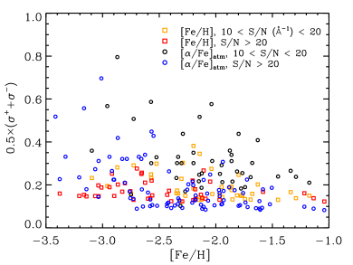
(a)

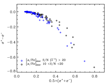
(b)

Figure 1.— Left: We plot the uncertainty in [Fe/H] and $[\alpha/\rm{Fe}]_{\rm{atm}}$  as a function of [Fe/H] for stars with S/N $>$ 20 Å^-1 and 10 $<$ S/N $<$ 20 Å^-1. In the case of $[\alpha/\rm{Fe}]_{\rm{atm}}$, we have averaged the $\sigma^{+}$ and $\sigma^{-}$ components for each measurement. The colors and plot symbols denote uncertainties in [Fe/H] or $[\alpha/\rm{Fe}]_{\rm{atm}}$ for different ranges of S/N. At a fixed S/N (Å^-1), $[\alpha/\rm{Fe}]_{\rm{atm}}$  uncertainties increase towards lower [Fe/H] due to progressively weaker features, whereas such a trend is not visible for [Fe/H], at least for those stars with $\sigma_{\rm{[Fe/H]}}<0.4$. The plot shows a minimum at $\sigma\sim{0.1}$ due to the element$-$dependent systematic uncertainty $\sigma_{\rm{sys}}$ added in quadrature to each random uncertainty. Right: We show the asymmetry between uncertainties $\sigma^{+}_{[\alpha/\rm{Fe}]_{\rm{atm}}}$ and $\sigma^{-}_{[\alpha/\rm{Fe}]_{\rm{atm}}}$ for the same data, defined as $\sigma^{+}-\sigma^{-}$, plotted as a function of the mean uncertainty (average of $\sigma^{+}$ and $\sigma^{-}$). The negative component $\sigma^{-}$ is generally equal or larger than $\sigma^{+}$. A similar trend is present for the individual $[\alpha_{\rm{j}}/\rm{Fe}]$  measurements.

Our technique consists of a pixel$-$by$-$pixel matching between each stellar spectrum and a finely$-$spaced grid of synthetic spectra optimized for our spectral wavelength range. To measure stellar parameters, we rely on the synthetic spectral grid synthesized by Kirby (2011) from plane$-$parallel ATLAS9 stellar atmospheres using the LTE abundance code MOOG (Sneden, 1973). In addition, we make use of an unpublished extension to the grid to measure individual alpha abundance ratios, as described in § 3.4.

The primary synthetic spectral grid has four dimensions: $T_{\rm{eff}}$, $\log g$, [Fe/H], and $[\alpha/\rm{Fe}]_{\rm{atm}}$. The quantity $[\alpha/\rm{Fe}]_{\rm{atm}}$  is defined as the $[\alpha/\rm{Fe}]$  abundance ratio of O, Ne, Mg, Si, S, Ar, Ca, and Ti used to synthesize each spectrum. The grid spans 3500 $\leq$ $T_{\rm{eff}}$  $\leq$ 8000 K, 0.0 $\leq$ $\log g$  $\leq$ 5.0, $-$5.0 $\leq$ [Fe/H] $\leq$ 0.0, and $-$0.8 $\leq$ [$\alpha$/Fe]_atm $\leq$ +1.2. Our sample is comprised of RGB stars ($\log g$  $<$ 3.6), making this grid sufficient for our analysis. The microturbulent velocity, $\xi$, used for each synthesis was determined using an empirical $\xi-\log g$ relation valid for RGB stars, derived from high$-$resolution spectroscopic measurements (Kirby et al. 2009, Equation 2).

We perform our analysis using only spectral regions with Fe, Mg, Si, Ca, or Ti features to maximize sensitivity to each element. The mask of usable spectral regions for a given element X is constructed by synthesizing three spectra with $\rm{[X/H]}=[-1.8,-1.5,-1.2]$, while all other abundances remained fixed at $\rm{[X/H]}=-1.5$. The mask is comprised of those wavelength segments where a 0.3 dex difference in [X/H] changes the normalized flux by $\gtrsim{0.5}\%$. To incorporate regions sensitive at a wide range of $T_{\rm{eff}}$ , the procedure was repeated at 1,000 K intervals between 4,000 K and 8,000 K, and the resulting masks joined. The Mg, Si, Ca and Ti element masks do not share wavelength segments in common, allowing us to measure individual abundances in § 3.4. The combined alpha mask is defined as the union of the Mg, Si, Ca, and Ti masks. We remove from the element masks spectral lines that are not modeled accurately by the LTE synthesis code, as determined by Kirby et al. (2008a) and listed in their Table 2. These include the Ca II triplet and the Mg I $\lambda{8807}$ feature. The Fe, Mg, Si, Ca, and Ti masks have roughly 222, 10, 20, 14, and 52 good segments each (i.e., not overlapping with telluric regions or with badly modeled spectral lines), where each segment corresponds to a spectral feature. The combined spectral widths of the wavelength segments for each element are $\sim{500}$, 16, 20, 14, and 52 Å, respectively.

3.2. $\chi^{2}$ Pixel$-$by$-$Pixel Matching

To perform the pixel fitting, we degrade the synthetic models to the DEIMOS spectral resolution. We account for a small quadratic dependence of the spectral FWHM on wavelength by fitting to unblended sky lines. We then convolve the synthetic spectra with this variable FWHM Gaussian kernel. For each star, we determine $\log g$  by fitting the SDSS photometry to a grid of Yale$-$Yonsei isochrones, as detailed in Kirby et al. (2010). The alternate spectroscopic approach, based on obtaining ionization equilibrium between Fe I and Fe II abundances, is not applicable to our data due to the dearth of absorption lines from ionized species in our red spectra. We normalize the flux$-$calibrated spectrum using a low order spline fit to wavelength regions not sensitive to any of Fe, Mg, Si, Ca or Ti. The normalization is later refined during the fitting process.

The best$-$fit parameters ($T_{\rm{eff}}$, [Fe/H], and $[\alpha/\rm{Fe}]_{\rm{atm}}$) and individual abundance ratios ($[\alpha_{\rm{j}}/\rm{Fe}]$, where $\alpha_{j}$ = Mg, Si, Ca and Ti in this work) are determined by minimizing the $\chi^{2}$ statistic between the rest$-$frame science spectrum and the convolved model grid in a multi$-$step process described by Kirby et al. (2010). We briefly describe the fitting procedure for the various stellar parameters and abundance ratios, highlighting the modifications implemented for this paper. In particular, we have updated our uncertainty analysis to provide more accurate asymmetric $[\alpha/\rm{Fe}]_{\rm{atm}}$  and $[\alpha_{\rm{j}}/\rm{Fe}]$  uncertainties. Throughout, we maintain the order of steps described in detail by Kirby et al. (2010).

3.3. $T_{\rm{eff}}$  and [Fe/H]

We fit $T_{\rm{eff}}$  and [Fe/H] simultaneously using the Fe mask. Due to the wavelength overlap between the Fe and combined alpha masks, we do not fit [Fe/H] and $[\alpha/\rm{Fe}]_{\rm{atm}}$  simultaneously. In order to optimize the fitting process in the two dimensional $T_{\rm{eff}}$$-$[Fe/H] parameter space, we perform the $\chi^{2}$ minimization using the code mpfit (Markwardt, 2009), which is an IDL implementation of the Levenberg$-$Marquardt $\chi^{2}$ algorithm.

We determine the random uncertainty in [Fe/H], $\sigma_{\rm{[Fe/H],ran}}$, by using the covariant error matrix of $T_{\rm{eff}}$  and [Fe/H] calculated by mpfit. Due to the non$-$zero cross$-$terms, $\sigma_{\rm{[Fe/H],ran}}$ is larger than if the [Fe/H] uncertainty was calculated by varying [Fe/H] alone. The total uncertainty in [Fe/H], $\sigma_{\rm{[Fe/H]}}$, is equal to the addition in quadrature of $\sigma_{\rm{[Fe/H],ran}}$ to a systematic uncertainty component $\sigma_{\rm{[Fe/H],sys}}$. Kirby et al. (2010) estimated $\sigma_{\rm{[Fe/H],sys}}$ by calculating the residual difference between DEIMOS and high$-$resolution abundances of globular cluster stars, after accounting for the random uncertainty in both sets of measurements added in quadrature. In order to check the reliability of the mpfit$-$derived uncertainties, we calculate $\chi^{2}$ around the best$-$fit $T_{\rm{eff}}$  and [Fe/H]. We find that $\chi^{2}$ contours for $T_{\rm{eff}}$  and [Fe/H] are symmetric about the minimum $\chi^{2}$ value for $\sigma_{\rm{[Fe/H]}}\lesssim{0.4}$, justifying our use of the symmetric mpfit random uncertainties. Henceforth, we only include stars with $\sigma_{\rm{[Fe/H]}}\leq{0.4}$.

3.4. $[\alpha/\rm{Fe}]_{\rm{atm}}$  and $[\alpha_{\rm{j}}/\rm{Fe}]$  Abundance Ratios

We calculate $[\alpha/\rm{Fe}]_{\rm{atm}}$  while fixing $T_{\rm{eff}}$  and [Fe/H] to the best$-$fit values, using the combined alpha mask defined in § 3.1. We compute $\chi^{2}$ contours for $[\alpha/\rm{Fe}]_{\rm{atm}}$  by measuring the sum of the pixel$-$to$-$pixel variation between the stellar spectrum and the primary spectral grid. We measure the best$-$fit $[\alpha/\rm{Fe}]_{\rm{atm}}$  value by finding the value corresponding to the minimum in the $\chi^{2}$ contour. The measurement of best$-$fit $[\alpha/\rm{Fe}]_{\rm{atm}}$  is analogous to that of Kirby et al., who performed this optimization using mpfit. After all stellar parameters ($T_{\rm{eff}}$, [Fe/H], and $[\alpha/\rm{Fe}]_{\rm{atm}}$) have converged to their best$-$fit values, we fit for the individual alpha abundances while keeping all stellar parameters fixed.

To measure individual $[\alpha_{\rm{j}}/\rm{Fe}]$  abundance ratios, we compare each spectrum to a supplementary spectral grid that samples values of $[\alpha_{\rm{j}}/\rm{Fe}]$  from $-0.8$ to $+1.2$ dex, while keeping all other abundances and stellar parameters fixed. The grid was synthesized only for spectral regions included within each $[\alpha_{\rm{j}}/\rm{Fe}]$  mask. We compute $\chi^{2}$ contours for each $[\alpha_{\rm{j}}/\rm{Fe}]$  by measuring the pixel$-$to$-$pixel variation between each spectrum and the supplementary spectral grid, instead of the primary grid.

In contrast to [Fe/H], we find that a significant number of $[\alpha/\rm{Fe}]_{\rm{atm}}$  and $[\alpha_{\rm{j}}/\rm{Fe}]$  contours are asymmetric about $\chi^{2}_{\rm{min}}$. We therefore estimate the random uncertainties by finding the two abundance values corresponding to $\chi^{2}_{\rm{min}}$ + 1 without assuming symmetry. We refer to the positive and negative difference between these values and the best$-$fit abundance ratio, $[\alpha/\rm{Fe}]$  as $\sigma^{+}_{[\alpha/\rm{Fe}]}$ and $\sigma^{-}_{[\alpha/\rm{Fe}]}$, respectively, where $[\alpha/\rm{Fe}]$  stands for any of $[\alpha/\rm{Fe}]_{\rm{atm}}$  or $[\alpha_{\rm{j}}/\rm{Fe}]$.

We also account for non$-$random errors due to, e.g., uncertainties in the other stellar parameters, by introducing a systematic error floor different for each abundance ratio, $\sigma_{[\alpha/\rm{Fe}]\,\rm{sys}}$, measured by Kirby et al. (2010) in the same way as $\sigma_{\rm{[Fe/H],sys}}$ (§ 3.3). The systematic uncertainties for $[\alpha/\rm{Fe}]_{\rm{atm}}$  [Mg/Fe], [Si/Fe], [Ca/Fe] and [Ti/Fe] are 0.08, 0.11, 0.18, 0.09, and 0.10 dex, respectively. We calculate the total uncertainty by adding $\sigma_{[\alpha/\rm{Fe}]\,\rm{sys}}$ to the $\sigma^{+}_{[\alpha/\rm{Fe}]\,\rm{ran}}$ and $\sigma^{+}_{[\alpha/\rm{Fe}]\,\rm{ran}}$ random components in quadrature. We note that $\sigma_{[\alpha/\rm{Fe}]\,\rm{sys}}$ only contributes significantly to the error budget when the random uncertainty is $\lesssim{0.1}$ dex.

All abundances are referenced to the Asplund et al. (2009) solar abundance scale. The offsets between the abundance scale used by Kirby et al. (2008b, 2010) and this work are minimal: $+0.02$, $-0.04$, $+0.02$, $+0.00$, $+0.02$ dex for [Fe/H], [Mg/Fe], [Si/Fe], [Ca/Fe], and [Ti/Fe], respectively, in the sense of this work minus Kirby et al. There is no difference in the mean $[\alpha/\rm{Fe}]_{\rm{atm}}$  between the old and new abundance scales.

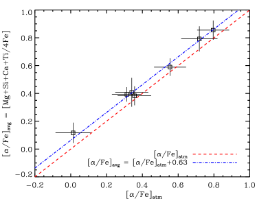
Figure 2.— We plot [$\alpha$/Fe]_atm against $[\alpha/\rm{Fe}]_{\rm{avg}}$  the mean of [Mg/Fe], [Si/Fe], [Ca/Fe], [Ti/Fe] for the nine stars with measurements available for all elements. The dashed (red) line is the $y=x$ line. The small offset between the data and the red line suggests a small difference between $[\alpha/\rm{Fe}]_{\rm{atm}}$  $[\alpha/\rm{Fe}]_{\rm{avg}}$. The mean vertical offset is +0.063 dex. The dot$-$dash (blue) line shows the improved agreement obtained after adding the offset to $[\alpha/\rm{Fe}]_{\rm{atm}}$. We thus define $[\alpha/\rm{Fe}]_{\rm{avg}}$  as $[\alpha/\rm{Fe}]_{\rm{atm}}$ $+0.63$, and apply this correction to all stars in our sample.

We show the uncertainty in [Fe/H] and $[\alpha/\rm{Fe}]_{\rm{atm}}$  for all UFD stars in the left panel of Figure 1. At a fixed S/N, the uncertainty increases towards lower [Fe/H] due to progressively weaker spectral features. The right panel shows the associated asymmetry in the $[\alpha/\rm{Fe}]_{\rm{atm}}$  uncertainty as a function of its average value. We find that $\sigma^{-}_{[\alpha/\rm{Fe}]_{\rm{atm}}}$ is preferentially larger than $\sigma^{+}_{[\alpha/\rm{Fe}]_{\rm{atm}}}$, with a similar effect present for each $[\alpha_{\rm{j}}/\rm{Fe}]$  (not shown in the figure). In our analysis, we include only abundances with $\sigma_{\rm{[Fe/H]}}\leq{0.4}$ and $\sigma^{+}_{[\alpha/\rm{Fe}]_{\rm{atm}}}$ $\leq$ 0.4 dex ($\sigma^{+}_{[\alpha_{\rm{j}}/\rm{Fe}]}$ $\leq$ 0.4 dex.) The final sample includes 61, 10, 34, 45, and 36  measurements of $[\alpha/\rm{Fe}]_{\rm{atm}}$, [Mg/Fe], [Si/Fe], [Ca/Fe], and [Ti/Fe], respectively.

In addition to the individual $[\alpha_{\rm{j}}/\rm{Fe}]$ , we report an overall alpha abundance ratio, which we denote as $[\alpha/\rm{Fe}]_{\rm{avg}}$. There is no homogeneous definition of $[\alpha/\rm{Fe}]_{\rm{avg}}$  in the literature. Different authors use different combinations of $[\alpha_{\rm{j}}/\rm{Fe}]$  to estimate $[\alpha/\rm{Fe}]_{\rm{avg}}$. We choose [$\alpha$/Fe]_atm as our initial estimate of $[\alpha/\rm{Fe}]_{\rm{avg}}$  because it was measured using the combined alpha mask, thus being sensitive to Mg, Si, Ca and Ti. $[\alpha/\rm{Fe}]_{\rm{atm}}$  has the added advantage of being measurable even when individual $[\alpha_{\rm{j}}/\rm{Fe}]$  are not, because it is measured from the combined signal of four elements.

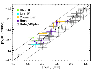
(a)

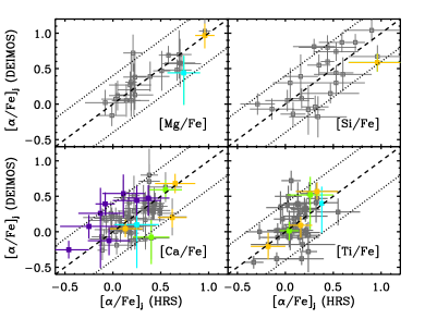
(b)

Figure 3.— Left: We compare our DEIMOS [Fe/H] measurements against published high$-$resolution (HRS) measurements in Com Ber, UMa II (Frebel et al., 2010), Leo IV (Simon et al., 2010), and Herc (Adén et al., 2011). We add to the comparison halo and classical dSphs stars presented in Kirby et al. (2010). Right: Comparison of [Mg/Fe], [Si/Fe], [Ca/Fe], and [Ti/Fe] abundance ratios for the same sample. The $[\alpha_{\rm{j}}/\rm{Fe}]$  abundance uncertainties for the UFD stars were measured as described in § 3.4. All measurements have been transformed to the Asplund et al. (2009) abundance scale. The dotted lines indicate a difference of $+0.4$ and $-0.4$ from equality, comparable to our largest allowed uncertainty. Both panels show good agreement between DEIMOS and HRS measurements. (see § 3.4).

In Figure 2, we compare [$\alpha$/Fe]_atm against the weighted mean of $[\alpha_{\rm{j}}/\rm{Fe}]$  for the nine stars with measurements for all elements. The comparison shows that [$\alpha$/Fe]_atm is offset relative to the weighted mean by $-0.063\pm{0.010}$ dex. We attribute this offset to the influence of the [Mg/Fe] measurements, which are systematically higher than [$\alpha$/Fe]_atm for all stars in this subsample. While the mean assigns equal weight to each element when the uncertainties are comparable, the measurement of [$\alpha$/Fe]_atm is less affected by the Mg abundance due to the relatively small number of Mg lines in the DEIMOS spectrum. We adjust the definition of $[\alpha/\rm{Fe}]_{\rm{avg}}$  as [$\alpha$/Fe]_atm + 0.063 dex in order to account for the systematic discrepancy described above.

We note that although use of an $[\alpha/\rm{Fe}]_{\rm{avg}}$  blurs nuanced differences that may be present between the different elements, it is a useful quantity because of the closely related nucleosynthetic origin of these elements. We report $[\alpha/\rm{Fe}]_{\rm{avg}}$  measurements for 61 stars (equal to the number of $[\alpha/\rm{Fe}]_{\rm{atm}}$  measurements) including seven stars for which no individual $[\alpha_{\rm{j}}/\rm{Fe}]$  were detect due to a lack of signal. Table 1 summarizes basic properties for each UFD, the number of stars with available $[\alpha/\rm{Fe}]$  measurements, and the weighed average metallicity for each UFD using only these stars.

3.5. Comparison with High$-$Resolution Studies

To validate our technique, we compare our results against high$-$resolution (HRS) abundances for overlapping stars in Com Ber, UMa II (Frebel et al., 2010), Leo IV (Simon et al., 2010), and Herc (Adén et al., 2011). Figure 3 shows the results of this comparison for [Fe/H] (left panel) and the individual $[\alpha_{\rm{j}}/\rm{Fe}]$  abundance ratios (right panel), where all abundances have been placed in the Asplund et al. (2009) abundance scale. Due to the small number of matching stars, we add to the comparison a set of halo stars with DEIMOS and high$-$resolution measurements analyzed by Kirby et al. (2010) using the same technique. We note that our modification to Kirby et al. (2010)’s approach lies in the determination of abundance uncertainties, and hence does not affect the comparison in Figure 3.

We find good agreement between [Fe/H] in both samples, with a mean difference of $-0.035\pm{0.022}$ dex in the sense HRS$-$DEIMOS, where the uncertainty is the standard error of the mean. The individual abundance ratios do not show any systematic offsets. The mean differences for [Mg/Fe], [Si/Fe], [Ca/Fe] and [Ti/Fe] are $+0.018\pm{0.035}$, $-0.005\pm{0.057}$, $-0.004\pm{0.029}$, and $0.022\pm{0.033}$ dex, respectively, demonstrating that we obtain accurate abundances over our entire range of values.

Table 1UFD Basic Data

UFD	R${}_{\rm{helio}}^{a}$    (kpc)	V${}_{\rm{rad}}^{b}$ (km/s)	$\sigma_{\rm{V}}^{b}$ (km/s)	M${}_{{V}}{}^{c}$	NMg	NSi	NCa	NTi	N${}_{[\alpha/\rm{Fe}]_{\rm{avg}}}$	$\langle\rm{[Fe/H]}\rangle^{d}$
Segue 1	23	208 $\pm$ 0.9	3.7 $\pm$ 1.4	$-$1.5	3	4	5	4	5	$-2.03\pm 0.06$
Coma Berenices	44	98 $\pm$ 0.9	4.6 $\pm$ 0.8	$-$4.1	1	5	7	4	9	$-2.53\pm 0.06$
Ursa Major II	32	$-$116 $\pm$ 1.9	6.7 $\pm$ 1.4	$-$4.2	2	5	4	4	6	$-2.15\pm 0.06$
Canes Venatici II	151	$-$128 $\pm$ 1.2	4.6 $\pm$ 1.0	$-$4.9	1	2	4	5	8	$-2.18\pm 0.06$
Leo IV	158	132 $\pm$ 1.4	3.3 $\pm$ 1.7	$-$5.0	0	4	2	4	4	$-2.89\pm 0.11$
Ursa Major I	106	$-$55 $\pm$ 1.4	7.6 $\pm$ 1.0	$-$5.5	2	7	9	8	11	$-2.04\pm 0.05$
Hercules	138	45 $\pm$ 1.1	5.1 $\pm$ 0.9	$-$6.6	1	5	13	3	13	$-2.42\pm 0.05$
Leo T	417	38 $\pm$ 2.0	7.5 $\pm$ 1.6	$-$7.1	0	2	1	4	5	$-1.94\pm 0.08$

4. Abundance Results I: Individual UFDs

The alpha abundances reflect the enrichment from SNe, and thus help constrain the underlying star formation history of a galaxy. In this section, we highlight the most salient qualitative trends for each UFD. We present the abundance measurements for all eight UFDs in Table 2. Figure 4 shows the $[\alpha/\rm{Fe}]_{\rm{avg}}$$-$[Fe/H] trends for each UFD in our sample, in order of increasing luminosity. The stars in each of our UFDs spans a range in metallicity greater than 1 dex. We discuss the implications of these trends in § 6.1.

Segue 1.$-$ Seg 1 is the faintest and nearest UFD known to date. We measure $[\alpha/\rm{Fe}]$  abundances for the 5 stars for which S11 reports metallicities (excluding the star with only an upper metallicity limit, [Fe/H] $<-3.4$). In spite of its low luminosity, the spread in metallicity is remarkably large, spanning $\gtrsim{2}$ dex from our 5 stars alone. The $[\alpha/\rm{Fe}]_{\rm{avg}}$  abundance ratios do not show any noticeable decrease with [Fe/H] and are roughly constant at $\sim{+0.6}$ dex; a similar trend is seen in [Ca/Fe]. The two stars at $\rm{[Fe/H]}\sim{-1.6}$ have slightly lower [Si/Fe] and [Ti/Fe] abundances than the two stars at $\rm{[Fe/H]}\sim{-2.4}$ (only by $\sim{0.15}$). In summary, Seg 1 shows enhanced abundance ratios even up to [Fe/H]$\sim{-1.6}$, suggestive of a lack of pollution by Type Ia SNe. The only published $[\alpha/\rm{Fe}]$  abundance ratios in Seg 1 are those of Norris et al. (2010b). Using high$-$resolution, they report [Mg/Fe] = +0.94, [Si/Fe] = +0.80, [Ca/Fe] = + 0.84, and [Ti II/Fe] = +0.65 for a [Fe/H] = $-$3.52 CEMP-no star (not in our sample). Their measurement agrees with the abundances measured in our most metal$-$poor star, which has a comparable metallicity.

Coma Berenices.$-$ Although there is no published constraint on its age spread, Com Ber’s CMD appears consistent with a very old age, with no intermediate age stars (Figure 3 of Muñoz et al. 2010). Com Ber shows high $[\alpha/\rm{Fe}]_{\rm{avg}}$ , greater than $+0.4$, at lower [Fe/H] and lower $[\alpha/\rm{Fe}]_{\rm{avg}}$  by $\sim{0.4}$ dex for the two highest [Fe/H] stars. [Si/Fe] and [Ca/Fe] also appear higher towards lower [Fe/H]. We do not detect any clear trend in [Ti/Fe], and there is insufficient data for [Mg/Fe]. Using high$-$resolution spectroscopy, Frebel et al. (2010) also reported enhanced alpha abundances at [Fe/H] $<-2.5$, whereas their most metal$-$rich star shows systematic lower $[\alpha/\rm{Fe}]$  abundance ratios by $\sim{0.4}$ dex. Their results show broad agreement with ours.

Ursa Major II.$-$ As for Com Ber, the CMD of UMa II is suggestive of a very old stellar population with no intermediate age stars (Muñoz et al., 2010). In contrast to Com Ber, UMa II shows signs of tidal stripping, suggesting it may have originally been a more luminous satellite. All of our $[\alpha/\rm{Fe}]_{\rm{avg}}$  measurements cluster at $[\alpha/\rm{Fe}]_{\rm{avg}}$$\sim{+0.4}$, spanning a large range of metallicities up to $\rm{[Fe/H]}\sim{-1.1}$. The three most metal$-$poor stars are overabundant in [Si/Fe] by $\sim{0.3}$ relative to the rest of the sample. Except for [Si/Fe], other abundance ratios appear to have flat abundance patterns. Frebel et al. (2010)’s measurements of three stars are in agreement with our result. They show roughly constant abundance ratios for [Mg/Fe], [Ca/Fe], and [Ti/Fe] for their three stars, all with [Fe/H] $<-2.3$. We measure $\rm{[Si/Ca]}=+1.17\pm{0.37}$ for a single star, which was also studied by Frebel et al. (2010) (their UMa$-$S2). They only measure an upper limit on [Si/Fe], $\rm{[Si/Fe]}<+1.46$. In combination with their [Ca/Fe] measurement, their upper limit for [Si/Ca] is $+1.08$, in agreement with our measurement. We defer the discussion of anomalous abundance ratios to § 5.3.

Canes Venatici II.$-$ The next five UFDs are at considerably larger distances than the previous three (see Table 1). Ground$-$based photometry suggests that CVn II is composed exclusively of an old ($>$ 10 Gy) stellar population (Sand et al., 2012; Okamoto et al., 2012). We present for the first time $[\alpha/\rm{Fe}]$  abundance ratios for this galaxy. At $\rm{[Fe/H]}<-2$, we find both high and low $[\alpha/\rm{Fe}]_{\rm{avg}}$  abundance ratios, hinting at some intrinsic scatter. On average, $[\alpha/\rm{Fe}]_{\rm{avg}}$  is higher at lower [Fe/H]. The distribution of [Ca/Fe] and [Ti/Fe] abundance ratios tentatively supports the presence of significant scatter at low [Fe/H].

Leo IV.$-$ Brown et al. (2012) have recently constrained the spread of ages of the stellar population to less than $\sim{2}$ Gyr. We have measured $[\alpha/\rm{Fe}]_{\rm{avg}}$  for four stars, which are consistent with either a shallow increase in $[\alpha/\rm{Fe}]_{\rm{avg}}$  with decreasing [Fe/H], or a constant enhancement of $\sim{0.3}$ dex. [Si/Fe] shows some evidence for slightly higher abundance ratios, $>0.5$ dex, but again no trend with [Fe/H] can be discerned. [Ti/Fe] is likewise relatively high. [Ca/Fe], measured in only two stars, is comparable to $[\alpha/\rm{Fe}]_{\rm{avg}}$. We note that the larger uncertainties in all abundance ratios (relative to other UFDs) are due to the low S/N of the DEIMOS spectra for this satellite. In agreement with our result, Simon et al. (2010) report enhanced $[\alpha/\rm{Fe}]$  abundance ratios for the brightest RGB, Leo IV S1. This star is also included in our sample; a comparison of the abundance ratios can be seen in Figure 3.

Table 2Abundance Results

UFD	RA (J2000)	DEC (J2000)	[Fe/H]	$[\alpha/\rm{Fe}]_{\rm{avg}}$	[Mg/Fe]	[Si/Fe]	[Ca/Fe]	[Ti/Fe]
Seg 1	$10:06:52.33$	$+16:02:35.8$	$-$3.42$\pm$0.28	+0.70${}^{+0.29}_{-0.74}$			+0.76${}^{+0.29}_{-0.53}$
Seg 1	$10:07:10.08$	$+16:06:23.9$	$-$1.61$\pm$0.12	+0.62${}^{+0.09}_{-0.09}$	+0.70${}^{+0.12}_{-0.14}$	+0.68${}^{+0.12}_{-0.14}$	+0.58${}^{+0.13}_{-0.13}$	+0.39${}^{+0.11}_{-0.13}$
Seg 1	$10:07:14.58$	$+16:01:54.5$	$-$1.59$\pm$0.12	+0.42${}^{+0.09}_{-0.09}$	+0.43${}^{+0.14}_{-0.14}$	+0.52${}^{+0.12}_{-0.11}$	+0.33${}^{+0.14}_{-0.17}$	+0.25${}^{+0.12}_{-0.13}$
Seg 1	$10:07:42.71$	$+16:01:06.9$	$-$2.43$\pm$0.13	+0.78${}^{+0.10}_{-0.10}$	+0.87${}^{+0.20}_{-0.31}$	+0.99${}^{+0.14}_{-0.13}$	+0.59${}^{+0.14}_{-0.14}$	+0.71${}^{+0.15}_{-0.19}$
Seg 1	$10:07:02.46$	$+15:50:55.2$	$-$2.32$\pm$0.15	+0.64${}^{+0.12}_{-0.13}$		+0.74${}^{+0.17}_{-0.25}$	+0.66${}^{+0.19}_{-0.19}$	+0.58${}^{+0.20}_{-0.29}$
Com Ber	$12:26:29.01$	$+24:04:03.8$	$-$2.52$\pm$0.29	+0.89${}^{+0.26}_{-0.40}$
Com Ber	$12:26:45.14$	$+23:50:44.7$	$-$2.92$\pm$0.22	+0.67${}^{+0.23}_{-0.30}$		+1.07${}^{+0.24}_{-0.33}$	+0.26${}^{+0.34}_{-0.71}$	+0.76${}^{+0.31}_{-0.69}$
Com Ber	$12:26:55.46$	$+23:56:09.8$	$-$2.70$\pm$0.12	+0.86${}^{+0.09}_{-0.09}$	+0.97${}^{+0.17}_{-0.18}$	+1.20${}^{+0.11}_{-0.12}$	+0.68${}^{+0.14}_{-0.14}$	+0.57${}^{+0.13}_{-0.11}$
…	…	…	…	…	…	…

Note. — Table 2 is published in its entirety in the electronic edition of the Astrophysical Journal. A portion is shown here for guidance regarding its form and content.

Ursa Major I.$-$ Brown et al. (2012) have shown that the stellar population is ancient, and constrained the spread in ages to less than $\sim{2}$ Gyr. We present the first $[\alpha/\rm{Fe}]$  abundance ratios measured in UMa I. The $[\alpha/\rm{Fe}]_{\rm{avg}}$  abundance pattern for UMa I shows on average increasing $[\alpha/\rm{Fe}]_{\rm{avg}}$  abundance ratios towards lower [Fe/H], with the possible exception of [Ca/Fe]. There is a hint of increased intrinsic scatter in $[\alpha/\rm{Fe}]_{\rm{avg}}$  and [Ca/Fe] at low [Fe/H], indicating that this galaxy might have experienced inhomogeneous chemical enrichment.

Hercules.$-$ Brown et al. (2012) have constrained the age and age spread in star formation to be similar to that in Leo IV and UMa I. We present measurements of $[\alpha/\rm{Fe}]_{\rm{avg}}$  for 13 stars, currently the largest published sample of $[\alpha/\rm{Fe}]$  for this UFD. One of our stars has $\rm{[Mg/Ca]}=+0.72\pm{0.21}$. We discuss its abundance pattern further in § 5.3. Herc shows a clear trend for rising $[\alpha/\rm{Fe}]_{\rm{avg}}$, [Si/Fe], and [Ca/Fe] towards lower [Fe/H], with little scatter, reaching $[\alpha/\rm{Fe}]_{\rm{avg}}$$\sim{+0.5}$ at the lowest [Fe/H]. The $[\alpha/\rm{Fe}]_{\rm{avg}}$  enhancement seems systematically lower at fixed [Fe/H] than in Seg 1 and Com Ber. The data is insufficient to suggest any pattern in the case of [Mg/Fe] and [Ti/Fe]. Recently, Adén et al. (2011) reported high$-$resolution [Ca/Fe] abundance ratios for 10 RGB stars in Hercules (eight overlap with our sample) with [Ca/Fe] varying from $\sim{+0.3}$ at [Fe/H]$\sim{-3.1}$ to [Ca/Fe]$\sim{-0.5}$ at [Fe/H] $\sim{-2}$, concluding that Herc experienced very inefficient star formation. Our measurements confirm the trend of decreasing [Ca/Fe] with rising [Fe/H].

Leo T.$-$ Leo T (Irwin et al., 2007) is the only UFD with evidence for recent star formation (e.g., Weisz et al., 2012; Clementini et al., 2012). It also has a large amount of HI gas (Ryan-Weber et al., 2008). These two properties distinguish it from all the other UFDs in this study. We have measured $[\alpha/\rm{Fe}]_{\rm{avg}}$  for 5 stars, 4 of which cluster around [Fe/H]$\sim{-2}$. and have a range of $[\alpha/\rm{Fe}]_{\rm{avg}}$  from $\sim{-0.1}$ to $\sim{+0.7}$. The only element with $>2$ measurements is [Ti/Fe], which was measured for the 4 stars at [Fe/H]$\sim{-2}$. All [Ti/Fe] measurements cluster between $-0.1$ and $+0.3$ dex. The presence of low $[\alpha/\rm{Fe}]$  stars is expected for systems with extended star formation.

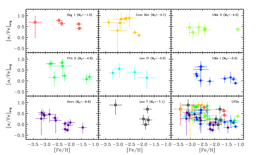
Figure 4.— $[\alpha/\rm{Fe}]_{\rm{avg}}$  as a function of [Fe/H] for each UFD in our sample, ordered by increasing galaxy luminosity. The bottom$-$right panel shows the combined UFD sample, also seen in Figure 5. Each UFD is assigned a different color. We use the same color scheme throughout the paper. Five of the UFDs have ancient stellar populations and show an overall decrease in $[\alpha/\rm{Fe}]_{\rm{avg}}$  with increasing [Fe/H]. We discuss their evolution in § 6.1.1. We use filled squares for stars in these galaxies and empty squares for the others. The presence of low $[\alpha/\rm{Fe}]_{\rm{avg}}$  stars at higher [Fe/H] strongly suggests that Type Ia SNe chemically enriched the ISM of these UFDs. Due to the time delay for Type Ia SNe after the onset of star formation, $t_{\rm{min,Ia}}$, our data suggests that most UFDs underwent at least a limited time period of extended chemical evolution, no shorter than $t_{\rm{min,Ia}}\sim 100$ Myr.

In summary, we observe the following trends for the individual UFDs:

• All UFDs have on average high $[\alpha/\rm{Fe}]$  abundance ratios ($\gtrsim{+0.3}$) at [Fe/H] $<-2.5$. High $[\alpha/\rm{Fe}]$  abundance ratios are consistent with chemical enrichment by Type II SNe.

• Most stars with [Fe/H] $>-1.5$ (excluding our Seg 1 and UMa II samples) have relatively low $[\alpha/\rm{Fe}]_{\rm{avg}}$  abundance ratios, $[\alpha/\rm{Fe}]_{\rm{avg}}$$<+0.4$, suggesting that chemical evolution lasted at least as long as the minimum time delay for Type Ia SNe.

• Seg 1 and UMa II are alpha$-$enhanced across their entire metallicity range. They do not show a statistically significant decrease in $[\alpha/\rm{Fe}]$  abundance ratios as a function of [Fe/H], in contrast to the other UFDs.

• The degree of alpha enhancement shows some hint of being different between UFDs, with Com Ber and Seg 1 having higher $[\alpha/\rm{Fe}]$  abundance ratios than Herc or UMa II at $\rm{[Fe/H]}\sim{-3}$. This could be a reflection of a different mix of SNe across the various UFDs, stochastic sampling of the same IMF, and/or inhomogeneous mixing.

5. Abundance Results II: The Ensemble of UFDs

A comparison of chemical abundances can shed light on the relationship between different stellar populations. It has been previously shown that the $[\alpha/\rm{Fe}]$ $-$[Fe/H] pattern in the classical dSphs disagrees with the Milky Way inner halo pattern for [Fe/H]$\gtrsim{-2}$. Building on this difference, simulations by Robertson et al. (2005) have suggested that the major building blocks of the inner halo had different star formation history than the extant classical dwarf galaxies.

Here, we compare the abundance patterns in our UFD sample against the inner halo, and also against one classical dSph, CVn I. With $\mathrm{M}_{\mathrm{V}}=-8.6$ (Martin et al., 2008b), CVn I is $\sim{2}$ magnitudes brighter than Leo T (the brightest UFD in our sample) and it is composed primarily of an old ($\gtrsim{10}$ Gy) population (Martin et al., 2008a; Okamoto et al., 2012). We use the CVn I sample from Kirby et al. (2010), reanalyzed to reflect our updated uncertainty analysis, which does not assume symmetric uncertainties (§ 3.4). We include the reanalyzed abundance measurements for CVn I (referenced to the Asplund et al. 2009 solar abundance scale) at the bottom of Table 2. The CVn I sample actually extends to $\rm{[Fe/H]}<-3$ and can be used as a comparison sample to the UFDs. For the halo, we rely on the chemical abundance compilation by Frebel (2010).

Since most of the UFDs have similar observed abundance trends, we merge the samples for the different UFDs to obtain a combined sample of more than 30 stars for each element, excluding Mg (due to very weak lines, Mg is only detectable in 10  stars). Figure 5 (left panels) compares the $[\alpha/\rm{Fe}]$  abundance ratios for our combined UFD sample against the inner halo population. For the halo sample, we calculated $[\alpha/\rm{Fe}]_{\rm{avg}}$  as the mean of the available [Mg/Fe], [Si/Fe], [Ca/Fe], and [Ti/Fe] abundance ratios. The right panels show a comparison of the $[\alpha/\rm{Fe}]$  abundance patterns of the more massive dSph CVn I against Milky Way inner halo stars. We explain our statistical comparison method in § 5.1, and describe the results in § 5.2. We comment on the presence of two stars with anomalous abundance ratios in § 5.3.

5.1. MCMC Modeling of Empirical $[\alpha_{\rm{j}}/\rm{Fe}]$$-$$\rm{[Fe/H]}$ Trends

In order to identify the best$-$fitting trend in $[\alpha/\rm{Fe}]$ $-$[Fe/H] space in a statistically robust way, we define simple parameterizations of the various trends predicted by chemical evolution models. In these models, the ISM is quickly enriched by ejecta from Type II SNe, resulting in high $[\alpha/\rm{Fe}]$  at low [Fe/H]. The onset of Type Ia SNe ejects more Fe$-$peak rich material and acts to lower $[\alpha/\rm{Fe}]$. Due to the delayed onset of Type Ia relative to Type II SNe, the change in $[\alpha/\rm{Fe}]$  can be seen as a turnover or knee at a particular [Fe/H]. Afterwards, the decrease in $[\alpha/\rm{Fe}]$  is modulated by the number of Type II and Type Ia SNe that explode. It is possible to increase $[\alpha/\rm{Fe}]$  with a late$-$time starburst (Gilmore & Wyse, 1991).

5.1.1 Empirical $[\alpha_{\rm{j}}/\rm{Fe}]$$-$$\rm{[Fe/H]}$ Models

We consider three simple models describing a path in $[\alpha_{\rm{j}}/\rm{Fe}]\,-\rm{[Fe/H]}$ space, where [Fe/H] and $[\alpha_{\rm{j}}/\rm{Fe}]$  are defined as the $x$ and $y$ coordinates. The ”Constant $[\alpha/\rm{Fe}]$  Model” (Model A) is a single$-$parameter model with a constant value of $[\alpha_{\rm{j}}/\rm{Fe}]$  at all [Fe/H], i.e. a flat line with $y=y_{0}$. It is representative of Type II SNe enrichment. The ”Single Slope Model” (Model B) is a two parameter linear model with freely$-$adjustable slope, $m=dy/dx$ and y$-$intercept, $b$, $y(x)=m\,x+b$. This model is representative of Type Ia SNe enrichment.

Equations 1$-$2 parameterize the ”Knee Model” (Model C), which is a combination of flat and decreasing $[\alpha_{\rm{j}}/\rm{Fe}]$  segments. It represents early Type II SNe enrichment followed by a phase where Type Ia SNe contributed to the chemical evolution.

$$y(x)=m\,{\rm{[Fe/H]_{0}}}+b\,;\,x\leq\rm{[Fe/H]_{0}}$$ (1)

$$y(x)=m\,x+b\,;\,x>\rm{[Fe/H]_{0}}$$ (2)

Here, $\rm{[Fe/H]}_{0}$ defines the boundary between the two segments, and is typically referred to as the knee. Parameters $m$ and $b$ are defined as in Model B.

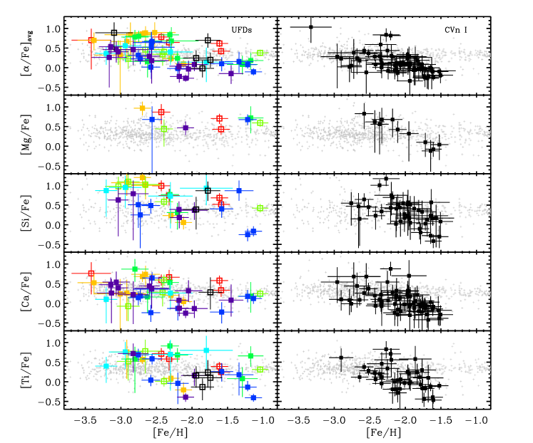
Figure 5.— We compare $[\alpha/\rm{Fe}]_{\rm{avg}}$  abundance ratios in the UFDs (left panels: filled/empty colored squares, same color and point scheme as in Figure 4), the Milky Way inner halo (small gray crosses in both panels), and the CVn I classical dSph (right panels: filled black squares). In the left panels, we ask whether the UFD population shares a similar abundance pattern as the inner halo. In the right panels, we compare CVn I and the inner halo. From top to bottom, we plot the $[\alpha/\rm{Fe}]_{\rm{avg}}$, [Mg/Fe], [Si/Fe], [Ca/Fe] & [Ti/Fe] abundance ratios. For the inner halo, we rely on the metal$-$poor star abundance compilation by Frebel (2010), with all abundances referenced to the Asplund et al. (2009) solar abundance scale. For CVn I, we use Kirby et al. 2010’s CVn I sample, reanalyzed using our updated analysis technique (§ 3). We qualitatively summarize the results of the statistical comparison described in § 5. Both the UFDs and CVn I show lower $[\alpha/\rm{Fe}]$  abundances than the inner halo at higher [Fe/H]. In addition, CVn I shows a hint of a turnover in $[\alpha/\rm{Fe}]$  at a metallicity between $-$2.5 and $-$2.0, not detected for the UFD sample (regardless of using the entire UFD sample, or the subsample marked with filled squares). This provides a hint that the (less luminous) UFDs underwent less efficient star formation than the classical dSphs, based on the non$-$detection of a turnover at $\rm{[Fe/H]}>-3$. Our data highlights that both UFDs and classical dSphs have a different chemical evolution than the inner halo.

5.1.2 Probability Distribution Functions for each Model

We seek to calculate the best$-$fit parameters and associated confidence intervals for each model given a dataset $\mathcal{D}$, where $\mathcal{D}$ is a set of [Fe/H] and $[\alpha_{\rm{j}}/\rm{Fe}]$ abundances. Due to our asymmetric uncertainties, we cannot rely on a simple regression analysis. For this purpose, we use a Markov$-$chain Monte Carlo method to calculate P ($\boldsymbol{\theta}$—$\mathcal{D}$), the joint probability density functions for each model as a function of its parameters $\boldsymbol{\theta}$ given $\mathcal{D}$. Specifically, we measure the probability density functions ${\rm{P}}_{\rm{A}}(y_{0})$, ${\rm{P}}_{\rm{B}}\,(m,k_{\rm{icpt}}$), and ${\rm{P}}_{\rm{C}}\,(m,k_{\rm{icpt}},\rm{[Fe/H]_{0}})$ for models A, B, and C. The primary input to the Markov chain are likelihoods for the full dataset $\mathcal{D}$ given a realization of $\boldsymbol{\theta}$, $\mathcal{L}(\mathcal{D}|\boldsymbol{\theta}$). This in turn requires calculating $\mathcal{L}$_i, the likelihood of star $i$ being drawn from the model.

Due to the non$-$Gaussian $[\alpha/\rm{Fe}]_{\rm{atm}}$  and $[\alpha_{\rm{j}}/\rm{Fe}]$  uncertainties discussed in §3.4, we make use of the probability distribution for each abundance to calculate $\mathcal{L}$_i. We denote these probability distributions as F, to avoid confusion with P ($\boldsymbol{\theta}$—$\mathcal{D}$). We compute the random component of F ($[\alpha_{\rm{j}}/\rm{Fe}]$) from the $\chi^{2}$ contours described in § 3.4. The probability of a star having abundance $y$ is given by Equation 3, and peaks at $\chi^{2}_{\rm{min}}$.

$${\rm{F_{ran}}}(y)\propto{}\exp{\left[-\frac{1}{2}\left(\chi^{2}(y)-\chi^{2}_{\rm{min}}\right)\right]}$$ (3)

We incorporate the systematic uncertainty in each measurement by convolving F_ran with a Gaussian with zero mean and standard deviation equal to $\sigma_{\rm{sys}}$. The full probability function for $[\alpha_{\rm{j}}/\rm{Fe}]$  is given in Equation 4.

$${\rm{F}}\,(y)=\displaystyle\int{{\rm{F_{ran}}}\,(y^{\prime})\frac{1}{\sqrt{2\pi\sigma^{2}_{\rm{sys}}}}{\rm{exp}}\left[-\frac{1}{2}\left(\frac{y-y^{\prime}}{\sigma_{sys}}\right)^{2}\right]\,dy^{\prime}}$$ (4)

In contrast to $[\alpha_{\rm{j}}/\rm{Fe}]$ , the [Fe/H] $\chi^{2}$ contours are symmetric for total uncertainties up to $\sigma_{\rm{[Fe/H]}}\sim{0.4}$ (§ 3.3). We thus define the probability distribution for [Fe/H], ${\rm{F}}\,(x)$, as a Gaussian with $\sigma_{\rm{[Fe/H]}}$, centered on the best$-$fit [Fe/H] value. We now calculate $\mathcal{L}$_i using Equation 5.

$$\mathcal{L}_{i}\,\propto\displaystyle\int{{\rm{F}}\,(x)\,{\rm{F}}\,(y\,(x))\,dx}$$ (5)

The full likelihood $\mathcal{L}(\mathcal{D}|\boldsymbol{\theta}$) is the product of the individual likelihoods for stars 1 $\leq$ $i$ $\leq$ N, $\mathcal{L}=\prod^{N}_{i=1}\mathcal{L}_{i}$. We run the Markov chain using the Metropolis-Hastings algorithm with a Gaussian$-$distributed kernel. We constrain [Fe/H]₀ to lie more than 0.3 dex away from the minimum in the sample, and below $\rm{[Fe/H]}=-2$. We chose this prior by noting that no knee has been observed in brighter dSphs at higher metallicities.

We constrain the slope in Models B and C to $m<0$. We run each chain for 100,000 steps for models A and B, and 250,000 steps for Model C. The larger number of steps is needed to better sample the larger parameter space in this model. In all cases, the first 1,000 steps are discarded as a burn$-$in period. For each step $k$, we compute the ratio of likelihoods $r\equiv\mathcal{L}_{k}/\mathcal{L}_{k-1}$ between the $k$ and $k-1$ steps

We accept the new set of parameters if $r>1$ or $0<\mathcal{U}\,(0,1)<r<1$, where $\mathcal{U}\,(0,1)$ is a uniform deviate between 0 and 1. Otherwise, we reject the trial step and save the parameters from step $k-1$ in step $k$.

The density of points in the chain defines P($\boldsymbol{\theta}|\mathcal{D}$). We determine the best$-$fit parameters from the peak of the one$-$dimensional probability distribution of each parameter. We determine the associated 68% Bayesian confidence intervals by constructing the cumulative probability function for each parameter and finding the parameters associated with values of 0.16 and 0.84 in the cumulative function. We then obtain an optimal set of parameters for each model, as well as an associated likelihood.

5.2. Abundances in the UFD vs the Inner Halo and the Classical dSphs

High$-$resolution studies have shown that local Milky Way halo stars (mostly belonging to the inner halo) have approximately constant $[\alpha_{\rm{j}}/\rm{Fe}]$  abundance ratios in the [Fe/H] range sampled by our data, $-$3.5 $<$ [Fe/H] $<$ $-$1.0 (e.g., McWilliam et al., 1995; Cayrel et al., 2004; Cohen et al., 2004). Figure 5 shows that the halo $[\alpha_{\rm{j}}/\rm{Fe}]$  is indeed flat in all four elements in our [Fe/H] range. In contrast, the classical dSphs are known to have lower $[\alpha/\rm{Fe}]$  at $\rm{[Fe/H]}\gtrsim{-2}$, while their $[\alpha/\rm{Fe}]$  abundance patters may broadly resemble the halo at $\rm{[Fe/H]}\lesssim{-3}$ (e.g., Cohen & Huang, 2010).

In order to compare the UFD abundance pattern to the halo and the dSphs, we use the technique described in § 5.1 to fit each of the three models to (a) a restricted sample of the five UFDs with ancient stellar populations and a trend of increasing $[\alpha/\rm{Fe}]$  with decreasing [Fe/H] (denoted by filled squares in Figure 4); (b) the full UFD sample; and (c) the CVn I sample. For each dataset, we obtain best$-$fitting Models A, B, and C, and the associated maximum likelihoods, $\mathcal{L_{A}\,,L_{B}\,,L_{C}}$. We then assess the goodness of fit between each of the best$-$fitting models. We note that these are nested models, such that Model A is a subset of Model B, itself a subset of Model C. We can thus use the likelihood ratio test in order to compare whether the more complex model is statistically a better fit that the simpler one. We compare two models at a time. Given the best$-$fit set of parameters for each of two models, e.g., A and B, the simpler model can be rejected at the $(1-\alpha)\times 100\%$ level using the inequality in Equation 6.

$$R_{\mathcal{B,A}}\equiv{}2\,ln\frac{\mathcal{L_{B}}}{\mathcal{L_{A}}}>F_{\chi}(\alpha;\,n_{B}-n_{A})=F_{\chi}(\alpha;\,k=1)$$ (6)

Here, $F_{\chi}(\alpha;\,n_{B}-n_{A})$, is the cumulative $\chi^{2}$ function with $n_{B}-n_{A}$ free parameters. In our case, $n_{B}-n_{A}=1$.

We report the likelihood ratio ($\mathcal{R}$ values) in Table 3. The best$-$fit models for the restricted UFD sample and the CVn I sample in the $[\alpha/\rm{Fe}]_{\rm{avg}}$ $-$[Fe/H] plane are presented in Figure 6. In both the CVn I and UFD panels, the blue band represents the range of slopes consistent within the joint 1$\sigma$ uncertainty contour of $m$ and $y_{0}$.

We first ask whether the UFD population has an abundance pattern consistent with the flat inner halo, using both the restricted and the full UFD sample. The Flat model can be ruled out at the 90% (99.5%) level if $\mathcal{R_{B,A}}\geq+2.7$ (+7.9). We measure $\mathcal{R_{B,A}}=6.02$ for [Ca/Fe] in the UFD restricted sample (+2.50 for the full sample), and $\mathcal{R_{B,A}}>10$ for [Si/Fe], [Ti/Fe], and $[\alpha/\rm{Fe}]_{\rm{avg}}$  for both samples, thus strongly ruling out the Flat model. This is also evident from a visual inspection of Figure 6 in the case of $[\alpha/\rm{Fe}]_{\rm{avg}}$. We have noted that only 10  stars have [Mg/Fe] measurements, and these are not evenly distributed among all UFDs. Hence we do not regard this fit as significant. We also perform a comparison of the Flat and Linear models for CVn I, and similarly conclude that the Linear model is a better fit than the Flat Model for all abundance ratios ($\mathcal{R_{B,A}}$ ranges from +5.78 to +48.66). Hence, both UFDs and brighter dSphs have alpha abundance patterns different than the Milky Way inner halo.

Next, we test the UFD sample and CVn I for the influence of Type Ia SNe enrichment by comparing the Linear Model against the Knee Model, which has one more free parameter. Again, we perform this test for the five UFDs with a clear $[\alpha/\rm{Fe}]$  trend, and for the full UFD sample. In both cases, the likelihood ratio test indicates that the UFD data is consistent with the Linear model (within the range of [Fe/H] of our data), so that adding a knee does not improve the fit. In contrast, we find that that the CVn I $[\alpha/\rm{Fe}]_{\rm{avg}}$  data is best$-$fit by a Knee model with a knee at [Fe/H] $=-2.45^{+0.13}_{-0.21}$ dex. The [Fe/H] value of the knee in the $[\alpha/\rm{Fe}]$, and [Si/Fe] plots agree within their 1$\sigma$ uncertainties. While the $\mathcal{R}_{C,B}$ value for $[\alpha/\rm{Fe}]_{\rm{avg}}$  suggests that a knee is present at this low [Fe/H], our data cannot rule out a model without a knee in the case of the individual alpha elements, for which $\mathcal{R}_{C,B}<2.2$. The hint of a knee in CVn I at [Fe/H] $>-2.5$ suggests that chemical evolution may not be a uniform process across dwarfs with different luminosities, since the population of fainter UFDs does not have a knee at [Fe/H] $\gtrsim{-3}$.

We caution that the crudeness of these toy models means that the evidence for a knee and flat abundance trend at lower [Fe/H] should be better interpreted broadly as evidence for a change in behavior in the $[\alpha/\rm{Fe}]$$-$[Fe/H] plane indicative of the onset of Type Ia SNe, and not as strictly ”flat” [$\alpha$/Fe] ratios at low metallicities. Even in the absence of Type Ia SNe, chemical enrichment likely depends on the mass of the progenitor Type II SNe (Woosley & Weaver, 1995; Nomoto et al., 2006). If the number of Type II SNe is small, then the first (most massive) SNe enrich the ISM with higher alpha abundance ratios, which then decrease as less massive SNe explode. This can result in a non$-$zero negative slope in $[\alpha/\rm{Fe}]$$-$[Fe/H], if the UFDs metallicity increases with time.

Table 3Relative Statistical Likelihood for Halo, Linear, and Knee Models

Element	$R_{\mathcal{B,A}}$ (UFDsa)	$R_{\mathcal{C,B}}$ (UFDsa)	$R_{\mathcal{B,A}}$ (UFDsb)	$R_{\mathcal{C,B}}$ (UFDsb)	$R_{\mathcal{B,A}}$ (CVn I)	$R_{\mathcal{C,B}}$ (CVn I)
$[\alpha$/Fe$]$	+29.82	$-$0.20	+10.70	$-$0.36	+48.66	+4.10
$[$Mg/Fe$]$	$-$0.72	$-$0.18	$-$0.68	$-$0.24	+5.78	$-$0.72
$[$Si/Fe$]$	+20.68	$-$0.36	+36.56	+0.18	+28.18	+2.24
$[$Ca/Fe$]$	+6.02	$-$0.10	+2.50	$-$0.14	+9.96	+1.40
$[$Ti/Fe$]$	+24.04	+0.08	+22.58	$-$0.16	+40.06	+0.54

Note. — Comparison of likelihood of best$-$fit parameters for the models discussed in § 5.2. Equation 6 defines $R_{x,y}$ for any two models $x$ and $y$. The letters A, B, and C stand for ”Flat Model”, ”Linear Model”, and ”Knee Model”. The best model fits for the UFDs^a and CVn I are presented in Figure 6.

Figure 6.— Top panel: Fits to models for $[\alpha/\rm{Fe}]_{\rm{avg}}\,-\rm{[Fe/H]}$ trends for the five UFDs with ancient stellar populations and increasing $[\alpha/\rm{Fe}]$  with decreasing [Fe/H] (shown with filled squares). The empty squares indicate stars in the three excluded UFDs (see Figure 4). Bottom panel: Fits to models for the CVn I dSph. The green (dashed), blue (solid), and red (dot$-$dashed) lines indicate the best$-$fitting ”Flat Model” (A), ”Linear Model” (B), and ”Knee Model” (C), respectively. The shaded blue band denotes the range of slopes within the joint 68% confidence region of the two parameters in the Linear Model. In the CVn I panel the best$-$fitting trend for the Knee Model is clearly distinct from the 68% band of the Linear Model. Using a likelihood ratio test applied to both models, we show that the Knee Model is significantly preferred over the Linear Model in the case of $[\alpha/\rm{Fe}]_{\rm{avg}}$  for CVn I The same test cannot distinguish between the Linear and Knee Models when applied to the combined UFD sample, even for $[\alpha/\rm{Fe}]_{\rm{avg}}$. The results are unchanged if using all eight UFDs. Thus, the UFD sample is consistent with rising $[\alpha/\rm{Fe}]_{\rm{avg}}$  towards lower [Fe/H], but its abundance pattern may differ from that of CVn I at $\rm{[Fe/H]}\lesssim{-2.5}$ and below. This suggests that chemical evolution is not universal at the faintest galaxy luminosities, since brighter systems, e.g. CVn I, appear to have a knee at higher [Fe/H] than the UFDs. The results of the likelihood ratio test are provided in Table 3.

5.3. Anomalous Abundance Ratios

Anomalous abundance ratios may be associated with enrichment from individual Type II SNe, given the mass$-$dependence of Type II SNe ejecta (e..g, Nomoto et al., 2006). Recent papers (e.g., Koch et al., 2008; Feltzing et al., 2009) have reported a few stars with anomalous abundance ratios, but the presence of such stars remains controversial (e.g., Gilmore et al. 2013 do not confirm the measurement by Feltzing et al. 2009). In the context of the UFDs studied here, Koch et al. (2008) reported a [Mg/Ca] = +0.94 star (their Her$-$2 object), and estimated its abundance pattern could be matched by the ejecta of a $\sim{35}\rm{M}_{\odot}$ Type II SN. We search our sample for anomalous [Mg/Ca] and [Si/Ca] abundance ratios. We conservatively define an abundance ratio between two alpha elements ([X/Y]) as anomalous if (a) the abundance ratio is more than 1$-\sigma$ greater than $+0.5$ or 1$-\sigma$ less than $-0.5$, and (b) the abundance ratio is discrepant by more than 1$-\sigma$ from the mean computed for the entire UFD sample, $\langle\rm{[X/Y]}\rangle$.

We tentatively identify anomalous abundance ratios in two stars, one of which is the object reported in Koch et al. (2008). Our measurement for that star is [Mg/Ca] $=+0.72\pm{0.21}$ at $\rm{[Fe/H]}=-2.09\pm{0.12}$. The mean [Mg/Ca] for the subsample with both [Mg/Fe] and [Ca/Fe] measurements is $\langle\rm{[Mg/Ca]}\rangle=+0.32\pm{.07}$ (error on the mean). We caution that only 10 stars have a [Mg/Fe] measurement, due to the weakness of Mg spectral features, making this subsample small. We also identify in UMa II a single star ([Fe/H]$=-2.90\pm{0.16}$) with an anomalous [Si/Ca] abundance ratio ($\rm{[Si/Ca]}=1.17\pm{0.37}$), where the mean [Si/Ca] ratio for our sample is $\langle\rm{[Si/Ca]}\rangle=+0.20\pm{.05}$. This star is also studied by Frebel et al. (2010) as UMa II$-$S2, but they only report an upper limit on [Si/Fe]. Using their [Si/Fe] upper limit and their [Ca/Fe] measurement, we obtain $\rm{[Si/Ca]}<+1.08$, consistent with our measurement. In total, we measure a moderately anomalous [Si/Ca] ratio in 1 out of 26 stars, and an anomalous [Mg/Ca] ratio in 1 out of 10 stars. Our results suggest that the fraction of stars with anomalous ratios of two alpha elements is small.

6. Discussion

6.1. Chemical Evolution in Individual UFDs

The distribution of alpha abundances allows to us to build a general picture of chemical evolution in the UFDs. The first explosions from Population III (Pop III) and/or massive Pop II stars provide the initial chemical enrichment of the UFD’s ISM, depositing large quantities of alpha elements into the gas from which later stars form. The low [Fe/H], high $[\alpha/\rm{Fe}]$  stars in our sample are formed from metal$-$enriched gas from these early SNe. This is a general feature in all of our UFDs. In contrast, our sample includes UFDs with and without low $[\alpha/\rm{Fe}]$  abundance ratios at high [Fe/H]. We note that the two dwarfs without low $[\alpha/\rm{Fe}]_{\rm{avg}}$  both have M${}_{V}>-4.2$. Hence, this distinction may still hint at a threshold for significant chemical evolution at M${}_{V}\sim-4$. However, Com Ber also has M${}_{V}>-4.2$ but does contain low $[\alpha/\rm{Fe}]_{\rm{avg}}$  stars. In addition to the general trend with [Fe/H], we note that there is a hint for an increase in scatter (beyond the observational uncertainties) in $[\alpha/\rm{Fe}]_{\rm{avg}}$  at lower [Fe/H]. This may hint towards inhomogeneous chemical enrichment (e.g., Argast et al., 2000; Oey, 2000), where the products of individual SNe contaminate different regions of the ISM without complete mixing. We discuss the two different abundance patterns in turn, but strongly caution that this distinction may only be the result of small samples for individual UFDs.

6.1.1 M${}_{V}<-4.2$ UFDs and Com Ber

Every bright UFD in our sample with M${}_{V}<-4.2$ (CVn II, Leo IV, UMa I, Herc, and Leo T) contain stars with solar or subsolar $[\alpha/\rm{Fe}]$  abundance ratios, the majority of which cluster at high [Fe/H]. The presence of low $[\alpha/\rm{Fe}]$  ratios is a strong indicator that star formation proceeded at least as long as needed for Type Ia SNe to explode. The minimum time delay between the onset of star formation and the first Type Ia SNe, $t_{\rm{min,Ia}}$, is not yet constrained precisely, but may be as short as $\sim{100}$ Myr (see review by Maoz & Mannucci 2012). In our discussion, we adopt $t_{\rm{min,Ia}}=100$ Myr. Thus, the low $[\alpha/\rm{Fe}]$  stars suggest that star formation in these UFDs lasted longer than $t_{\rm{min,Ia}}$, and that the first generation of Type II SNe does not succeed in quenching star formation in these systems. Additionally, the decrease in $[\alpha/\rm{Fe}]$  ratios at $\mbox{[Fe/H]}\sim{-2.5}$ suggest a very small level of self$-$enrichment prior to the onset of Type Ia SNe. This is consistent with a system with a very low star formation rate.

6.1.2 Seg 1 and UMa II (M${}_{V}>-4.2$)

The Seg 1 and UMa II UFDs are the only systems which do not show any low $[\alpha/\rm{Fe}]$  stars. This suggests that star formation lasted less than $\sim 100\,\rm{Myr}$. In contrast to all other UFDs, the high $[\alpha/\rm{Fe}]$  stars extend to much higher [Fe/H]. Such high [Fe/H] stars are difficult to explain using the trends found for the other UFDs, i.e. systems with low star formation efficiencies. Frebel & Bromm (2012) have recently described a scenario for such one$-$shot chemical enrichment. In this picture, after the first Pop III stars, there is a single epoch of star formation, after which all gas is blown out of the system by SNe feedback or reionization. In this picture, the large spread in [Fe/H] arises from highly inhomogeneous gas mixing, as also pointed out by Argast et al. (2000) and Oey (2000). Large [Fe/H] spreads can perhaps instead be the result of accretion of multiple progenitor systems, each with a different metallicity (Ricotti & Gnedin, 2005). An alternative explanation for the early loss of gas before $t_{\rm{min,Ia}}$ is gas stripping due to accretion onto the Milky Way. We thus consider in more detail the different possibilities for the quenching of star formation, taking into account our $[\alpha/\rm{Fe}]$  results for each UFD.

6.2. Quenching of Star Formation

We saw above that UMa II and Seg 1 show hints of truncated star formation. If this is due to gas stripping due to accretion into the Milky Way, then the time of accretion into the halo should be comparable to the time of star formation quenching. Recently, Rocha et al. (2012) have studied the relation between time of infall and present$-$day galactocentric position and line$-$of sight velocities of subhalos in the Via Lactea 2 simulation, calculating the probability distribution of the infall time for UFDs and classical dSphs (their Figure 4). Interestingly, only Seg 1 and UMa II, the two UFDs with flat $[\alpha/\rm{Fe}]-$[Fe/H] patterns, show a significant probability of infall onto the Milky Way halo more than 12 ago (Com Ber may have an infall time as old as $\sim{11}$ Gyr ago). The early infall suggests that gas stripping and/or heating due to accretion played a role in terminating star formation before low $[\alpha/\rm{Fe}]$ stars could form. However, the presence of high [Fe/H] stars poses a problem to this interpretation, since the presence of high $[\alpha/\rm{Fe}]$, high [Fe/H] stars is attributed to systems with high star formation efficiencies. Thus, it is also possible that internal effects, e.g., winds from SNe, managed to get rid of or heat all of the remaining cold gas reservoir.

In contrast to Seg 1 and UMa II, the other UFDs have inferred infall times younger than 10 Gyr (Rocha et al., 2012). Brown et al. (2012) have reported upper limits on the duration of star formation of less than $\sim{2}$ Gyr for three UFDs (UMa I, Herc, Leo IV), implying star formation was terminated in the first few Gyr after the Big Bang. Okamoto et al. (2012) also report a lack of a significant age spread in CVn II. Therefore, gas stripping due to accretion likely occurred only after quenching of star formation, thus limiting this process’s role in the chemical evolution of the majority of UFDs.

The presence of low $[\alpha/\rm{Fe}]$  abundance ratios suggests that star formation lasted for at least $\sim$100  Myr in most UFDs. Assuming that the first Pop III stars form $\sim{180}$ Myr ($z\sim{20}$) after the Big Bang (e.g., Abel et al., 2000), the end of star formation likely occurred after $z\sim{14.5}$. This approximate upper limit on the redshift at which quenching occurred changes depending on the actual minimum time delay for Type Ia SNe. If the minimum time delay for Type Ia SNe is on the order of 500 Myr instead (five times the value adopted above), then quenching happened no earlier than $z\sim{7.7}$. The process of reionization likely extends for an extended range in redshift: $14\lesssim{z}\lesssim{6}$ (Fan et al., 2006). Our data are thus consistent with either internal evolutionary processes, i.e. Type II SNe blowing out the gas or providing enough thermal feedback to suppress the formation of additional stars, or reionization$-$driven quenching (Bullock et al., 2000; Ricotti & Gnedin, 2005). In both scenarios, the effect of the first SNe explosions (from Pop III and/or massive Pop II stars) must still allow for star formation to proceed long enough for Type Ia SNe to explode and enrich the ISM.

6.3. The UFDs and the Halo

In § 5.2, we characterized the distribution of $[\alpha/\rm{Fe}]$  abundances as a function of [Fe/H]. We showed that the probability that this distribution is drawn from a flat, inner$-$halo-like abundance pattern is less than a few percent. This fully agrees with a picture where the bulk of the inner halo forms from the accretion of a few massive satellites undergoing efficient star formation (Robertson et al., 2005), rather than the UFDs.

The fractional contribution of stars to the halo from UFDs may rise towards lower metallicities. The Milky Way halo is known to host extremely metal$-$poor stars (EMPs) with $\rm{[Fe/H]}\leq{-3}$. In contrast to the classical dSphs, the UFDs host a significant fraction of EMPs. Our sample, which is not metallicity$-$biased, has 10  EMP stars out of 61. At these low [Fe/H], the similarity in alpha enhancement between the halo and the combined UFD sample alone does suggest a larger contribution of the UFDs or UFD$-$like systems to the low metallicity tail of the inner halo. Since star formation likely ceased in the UFDs significantly prior to being accreted into the Milky Way potential, it suggests that the present$-$day UFD abundance patterns may be similar to those of UFDs accreted in the past, so that a large population of UFDs with similar abundance patterns may have contributed to the build$-$up of the EMP inner halo. This picture will need to be refined and tested by comparing other species with different nucleosynthetic origins, such as neutron$-$capture elements. For example, high$-$resolution studies of small numbers of stars in the UFDs suggest that the mean [Ba/Fe] ratio in Com Ber (Frebel et al., 2010) is lower than in UMa II or Boötes I (Gilmore et al., 2013). In contrast to Com Ber, these two UFDs have [Ba/Fe] ratios more similar to those of the Milky Way inner halo at $\rm{[Fe/H]}\sim{-2.5}$.

As a final note, it is worth emphasizing that a comparison of UFD abundances to the outer halo may provide circumstantial evidence for a stronger link between these two populations. The few studies to date rely on kinematically selected, nearby halo stars consistent with outer halo membership based on their kinematics and/or calculated orbital motions (e.g., Fulbright, 2002; Roederer, 2009; Ishigaki et al., 2010). Nissen & Schuster (2010) in particular show a clearly distinguishable population of low $[\alpha/\rm{Fe}]$  stars in the range $-1.6<\rm{[Fe/H]}<-0.4$. These are likely outer halo stars with high eccentricities, which thus take them as close as the Solar radius. However, orbits calculated to date for a few dSphs (e.g., Piatek et al., 2005) show that their orbits are not likely to pass as close as the Solar Galactocentric radius. All UFDs are at present at least as far as $R_{\rm{GC}}\sim{28}$ kpc. Thus, a full understanding of the UFD/dSph$-$outer halo connection awaits a detailed mapping of chemical abundances in the in$-$situ outer halo.

7. Conclusions

We analyze Keck/DEIMOS spectroscopy of RGB stars in eight UFDs using a spectral matching technique to measure and characterize the distribution of $[\alpha/\rm{Fe}]$  abundance ratios. In this paper, we report [Mg/Fe], [Si/Fe], [Ca/Fe], and [Ti/Fe], as well as a combined alpha to Fe abundance ratio, $[\alpha/\rm{Fe}]_{\rm{avg}}$ , for 61  stars in these systems. We summarize our main conclusions as follows:

• Out of seven UFDs with ancient stellar populations, five (Coma Berenices, Canes Venatici II, Ursa Major I, Leo IV and Hercules) show an increase of $[\alpha/\rm{Fe}]$  towards lower [Fe/H], and low $[\alpha/\rm{Fe}]$  ratios for their highest [Fe/H] stars, implying that Type Ia SNe had enough time to pollute the ISM. This suggests that star formation was an extended process, lasting at least $\sim{100}$ Myr, corresponding to the minimum time delay between the onset of star formation and the first Type Ia SNe. Leo T, which has a much more extended star formation history, shows the same abundance pattern.

• The remaining two UFDs with old populations, Segue 1 and Ursa Major II, show enhanced $[\alpha/\rm{Fe}]$  ratios at all metallicities, ranging from $-3.5\lesssim{\rm{[Fe/H]}}\lesssim{-1.0}$. On average, the mean level of alpha$-$enhancement in Segue I is higher than in UMa II by $\sim{0.2}$ dex. The absence of low $[\alpha/\rm{Fe}]$  stars suggests that the star formation period was very short, less than $\sim 100$ Myr.

• The combined population of UFDs shows a clear increasing trend in $[\alpha/\rm{Fe}]$  with decreasing [Fe/H], with no evidence for a plateau within our entire metallicity range. Although this rise in $[\alpha/\rm{Fe}]$  disagrees with the flat inner halo abundance pattern, a significant number of $\rm{[Fe/H]}<-2.5$ stars in the UFDs have abundance ratios consistent with the halo values within the uncertainties. Therefore, the UFD contribution to the extremely metal$-$poor star (EMP) halo abundance pattern may be more significant at the lowest metallicities.

• The abundance pattern in the UFDs shows some difference with respect to the brighter CVn I dSph. We show that, in contrast to the UFD population, there is a hint for a plateau at [Fe/H]$\sim{-2.3}$ in CVn I. This difference suggests that the star formation efficiency in the UFDs was lower than in the more luminous dSphs.

We have shown based on $[\alpha/\rm{Fe}]$  abundance ratios that most of the UFDs were able to retain gas and form stars long enough for the first Type Ia SNe to explode, and that this evolution proceeded inefficiently. The use of medium$-$resolution spectroscopy has been instrumental in providing us with large enough samples to begin to address the evolution of these systems. Future studies will aim to study the details of this evolution by comparing the shape of the metallicity distribution function of each UFD to chemical evolution models. For instance, evidence for a rapid shutdown in star formation due to reionization may appear as an abrupt cutoff in the metallicity distribution function at the higher [Fe/H] end. Due to the sparseness of the RGBs of the UFDs, it will become necessary to extend the power of multiplex spectroscopic observations to the main sequence of the UFDs in order to obtain statistically significant samples to achieve this goal.

References

- Abel et al. (2000) Abel, T., Bryan, G. L., & Norman, M. L. 2000, ApJ, 540, 39
- Adén et al. (2011) Adén, D., Eriksson, K., Feltzing, S., et al. 2011, A&A, 525, A153
- Allende Prieto et al. (2006) Allende Prieto, C., Beers, T. C., Wilhelm, R., et al. 2006, ApJ, 636, 804
- Argast et al. (2000) Argast, D., Samland, M., Gerhard, O. E., & Thielemann, F.-K. 2000, A&A, 356, 873
- Asplund et al. (2009) Asplund, M., Grevesse, N., Sauval, A. J., & Scott, P. 2009, ARA&A, 47, 481
- Belokurov et al. (2006) Belokurov, V., Zucker, D. B., Evans, N. W., et al. 2006, ApJ, 647, L111
- Belokurov et al. (2007) Belokurov, V., Zucker, D. B., Evans, N. W., et al. 2007, ApJ, 654, 897
- Brown et al. (2012) Brown, T. M., Tumlinson, J., Geha, M., et al. 2012, ApJ, 753, L21
- Bullock et al. (2000) Bullock, J. S., Kravtsov, A. V., & Weinberg, D. H. 2000, ApJ, 539, 517
- Cayrel et al. (2004) Cayrel, R., Depagne, E., Spite, M., et al. 2004, A&A, 416, 1117
- Clementini et al. (2012) Clementini, G., Cignoni, M., Contreras Ramos, R., Federici, L., Ripepi, V., et al. 2012, ApJ, 756, 108
- Cohen et al. (2004) Cohen, J. G., Christlieb, N., McWilliam, A., et al. 2004, ApJ, 612, 1107
- Cohen & Huang (2010) Cohen, J. G. & Huang, W. 2010, ApJ, 719, 931
- Cooper et al. (2012) Cooper, M. C., Newman, J. A., Davis, M., Finkbeiner, D. P., & Gerke, B. F. 2012, Astrophysics Source Code Library, 3003
- Faber et al. (2003) Faber, S. M., Phillips, A. C., Kibrick, R. I., et al. 2003, Proc. SPIE, 4841, 1657
- Fan et al. (2006) Fan, X., Carilli, C. L., & Keating, B. 2006, ARA&A, 44, 415
- Feltzing et al. (2009) Feltzing, S., Eriksson, K., Kleyna, J., & Wilkinson, M. I. 2009, A&A, 508, L1
- Frebel (2010) Frebel, A. 2010, Astronomische Nachrichten, 331, 474
- Frebel & Bromm (2012) Frebel, A. & Bromm, V. 2012, ApJ, 759, 115
- Frebel et al. (2010) Frebel, A., Simon, J. D., Geha, M., & Willman, B. 2010, ApJ, 708, 560
- Fulbright (2002) Fulbright, J. P. 2002, AJ, 123, 404
- Geha et al. (2009) Geha, M., Willman, B., Simon, J. D., et al. 2009, ApJ, 692, 1464
- Gilmore et al. (2013) Gilmore, G., Norris, J. E., Monaco, L., et al. 2013, ApJ, 763, 61
- Gilmore & Wyse (1991) Gilmore, G. & Wyse, R. F. G. 1991, ApJ, 367, L55
- Irwin et al. (2007) Irwin, M. J., Belokurov, V., Evans, N. W., et al. 2007, ApJ, 656, L13
- Ishigaki et al. (2010) Ishigaki, M., Chiba, M., & Aoki, W. 2010, PASJ, 62, 143
- Kirby (2011) Kirby, E. N. 2011, PASP, 123, 531
- Kirby et al. (2011) Kirby, E. N., Cohen, J. G., Smith, G. H., et al. 2011, ApJ, 727, 79
- Kirby et al. (2009) Kirby, E. N., Guhathakurta, P., Bolte, M., Sneden, C., & Geha, M. C. 2009, ApJ, 705, 328
- Kirby et al. (2010) Kirby, E. N., Guhathakurta, P., Simon, J. D., et al. 2010, ApJS, 191, 352
- Kirby et al. (2008a) Kirby, E. N., Guhathakurta, P., & Sneden, C. 2008a, ApJ, 682, 1217
- Kirby et al. (2008b) Kirby, E. N., Simon, J. D., Geha, M., Guhathakurta, P., & Frebel, A. 2008b, ApJ, 685, L43
- Koch et al. (2008) Koch, A., McWilliam, A., Grebel, E. K., Zucker, D. B., & Belokurov, V. 2008, ApJ, 688, L13
- Lai et al. (2011) Lai, D. K., Lee, Y. S., Bolte, M., et al. 2011, ApJ, 738, 51
- Lanfranchi & Matteucci (2004) Lanfranchi, G. A. & Matteucci, F. 2004, MNRAS, 351, 1338
- Lee et al. (2011) Lee, Y. S., Beers, T. C., Allende Prieto, C., et al. 2011, AJ, 141, 90
- Lee et al. (2008) Lee, Y. S., Beers, T. C., Sivarani, T., et al. 2008, AJ, 136, 2022
- Maoz & Mannucci (2012) Maoz, D. & Mannucci, F. 2012, PASA, 29, 447
- Maoz et al. (2012) Maoz, D., Mannucci, F., & Brandt, T. D. 2012, MNRAS, 426, 3282
- Markwardt (2009) Markwardt, C. B. 2009, in ASP Conf. Ser. 411, Astronomical Data Analysis Software and Systems XVIII, ed. D. A. Bohlender, D. Durand, & P. Dowler (San Francisco: ASP), 251
- Martin et al. (2008a) Martin, N. F., Coleman, M. G., De Jong, J. T. A., et al. 2008a, ApJ, 672, L13
- Martin et al. (2008b) Martin, N. F., de Jong, J. T. A., & Rix, H.-W. 2008b, ApJ, 684, 1075
- McWilliam et al. (1995) McWilliam, A., Preston, G. W., Sneden, C., & Searle, L. 1995, AJ, 109, 2757
- Muñoz et al. (2010) Muñoz, R. R., Geha, M., & Willman, B. 2010, AJ, 140, 138
- Newman et al. (2012) Newman, J. A., Cooper, M. C., Davis, M., et al. 2012, ApJS, submitted
- Nissen & Schuster (2010) Nissen, P. E. & Schuster, W. J. 2010, A&A, 511, L10
- Nomoto et al. (2006) Nomoto, K., Tominaga, N., Umeda, H., Kobayashi, C., & Maeda, K. 2006, Nuclear Physics A, 777, 424
- Norris et al. (2010a) Norris, J. E., Gilmore, G., Wyse, R. F. G., Yong, D., & Frebel, A. 2010a, ApJ, 722, L104
- Norris et al. (2010b) Norris, J. E., Wyse, R. F. G., Gilmore, G., et al. 2010b, ApJ, 723, 1632
- Norris et al. (2010c) Norris, J. E., Yong, D., Gilmore, G., & Wyse, R. F. G. 2010c, ApJ, 711, 350
- Norris et al. (2013) Norris, J. E., Yong, D., Bessell, M. S., et al. 2013, ApJ, 762, 28
- Oey (2000) Oey, M. S. 2000, ApJ, 542, L25
- Okamoto et al. (2012) Okamoto, S., Arimoto, N., Yamada, Y., & Onodera, M. 2012, ApJ, 744, 96
- Pagel (2009) Pagel, B. E. J. 2009, Nucleosynthesis and Chemical Evolution of Galaxies (2nd ed.; Cambridge: Cambridge UP)
- Piatek et al. (2005) Piatek, S., Pryor, C., Bristow, P., et al. 2005, AJ, 130, 95
- Revaz et al. (2009) Revaz, Y., Jablonka, P., Sawala, T., et al. 2009, A&A, 501, 189
- Ricotti & Gnedin (2005) Ricotti, M., & Gnedin, N. Y. 2005, ApJ, 629, 259
- Robertson et al. (2005) Robertson, B., Bullock, J. S., Font, A. S., Johnston, K. V., & Hernquist, L. 2005, ApJ, 632, 872
- Rocha et al. (2012) Rocha, M., Peter, A. H. G., & Bullock, J. 2012, MNRAS, 425, 231
- Roederer (2009) Roederer, I. U. 2009, AJ, 137, 272
- Ryan-Weber et al. (2008) Ryan-Weber, E. V., Begum, A., Oosterloo, T., et al. 2008, MNRAS, 384, 535
- Sakamoto & Hasegawa (2006) Sakamoto, T. & Hasegawa, T. 2006, ApJ, 653, L29
- Sand et al. (2012) Sand, D. J., Strader, J., Willman, B., et al. 2012, ApJ, 756, 79
- Shetrone et al. (2001) Shetrone, M. D., Côté, P., & Sargent, W. L. W. 2001, ApJ, 548, 592
- Simon et al. (2010) Simon, J. D., Frebel, A., McWilliam, A., Kirby, E. N., & Thompson, I. B. 2010, ApJ, 716, 446
- Simon & Geha (2007) Simon, J. D. & Geha, M. 2007, ApJ, 670, 313
- Simon et al. (2011) Simon, J. D., Geha, M., Minor, Q. E., et al. 2011, ApJ, 733, 46
- Sneden (1973) Sneden, C. A. 1973, Ph.D. Thesis, The University of Texas at Austin
- Totani et al. (2008) Totani, T., Morokuma, T., Oda, T., Doi, M., & Yasuda, N. 2008, PASJ, 60, 1327
- Venn et al. (2004) Venn, K. A., Irwin, M., Shetrone, M. D., et al. 2004, AJ, 128, 1177
- Walsh et al. (2007) Walsh, S. M., Jerjen, H., & Willman, B. 2007, ApJ, 662, L83
- Weisz et al. (2012) Weisz, D. R., Zucker, D. B., Dolphin, A. E., et al. 2012, ApJ, 748, 88
- Willman et al. (2005a) Willman, B., Blanton, M. R., West, A. A., et al. 2005a, AJ, 129, 2692
- Willman et al. (2005b) Willman, B., Dalcanton, J. J., Martinez-Delgado, D., et al. 2005b, ApJ, 626, L85
- Wise et al. (2012) Wise, J. H., Turk, M. J., Norman, M. L., & Abel, T. 2012, ApJ, 745, 50
- Woosley & Weaver (1995) Woosley, S. E. & Weaver, T. A. 1995, ApJS, 101, 181
- Zucker et al. (2006a) Zucker, D. B., Belokurov, V., Evans, N. W., et al. 2006a, ApJ, 650, L41
- Zucker et al. (2006b) Zucker, D. B., Belokurov, V., Evans, N. W., et al. 2006b, ApJ, 643, L103