Variational Algorithms for Marginal MAP

\nameQiang Liu \emailqliu1@uci.edu
\addrDonald Bren School of Information and Computer Sciences
University of California, Irvine
Irvine, CA, 92697-3425, USA
\AND\nameAlexander Ihler \emailihler@ics.uci.edu
\addrDonald Bren School of Information and Computer Sciences
University of California, Irvine
Irvine, CA, 92697-3425, USA
Abstract

The marginal maximum a posteriori probability (MAP) estimation problem, which calculates the mode of the marginal posterior distribution of a subset of variables with the remaining variables marginalized, is an important inference problem in many models, such as those with hidden variables or uncertain parameters. Unfortunately, marginal MAP can be NP-hard even on trees, and has attracted less attention in the literature compared to the joint MAP (maximization) and marginalization problems. We derive a general dual representation for marginal MAP that naturally integrates the marginalization and maximization operations into a joint variational optimization problem, making it possible to easily extend most or all variational-based algorithms to marginal MAP. In particular, we derive a set of “mixed-product” message passing algorithms for marginal MAP, whose form is a hybrid of max-product, sum-product and a novel “argmax-product” message updates. We also derive a class of convergent algorithms based on proximal point methods, including one that transforms the marginal MAP problem into a sequence of standard marginalization problems. Theoretically, we provide guarantees under which our algorithms give globally or locally optimal solutions, and provide novel upper bounds on the optimal objectives. Empirically, we demonstrate that our algorithms significantly outperform the existing approaches, including a state-of-the-art algorithm based on local search methods.

Keywords: Graphical Models, Message Passing, Belief Propagation, Variational Methods, Maximum a Posteriori, Marginal-MAP, Hidden Variable Models.

1 Introduction

Graphical models such as Bayesian networks and Markov random fields provide a powerful framework for reasoning about conditional dependency structures over many variables, and have found wide application in many areas including error correcting codes, computer vision, and computational biology (Wainwright and Jordan, 2008; Koller and Friedman, 2009). Given a graphical model, which may be estimated from empirical data or constructed by domain expertise, the term inference refers generically to answering probabilistic queries about the model, such as computing marginal probabilities or maximum a posteriori estimates. Although these inference tasks are NP-hard in the worst case, recent algorithmic advances, including the development of variational methods and the family of algorithms collectively called belief propagation, provide approximate or exact solutions for these problems in many practical circumstances.

In this work we will focus on three common types of inference tasks. The first involves maximization or max-inference tasks, sometimes called maximum a posteriori (MAP) or most probable explanation (MPE) tasks, which look for a mode of the joint probability. The second are sum-inference tasks, which include calculating the marginal probabilities or the normalization constant of the distribution (corresponding to the probability of evidence in a Bayesian network). Finally, the main focus of this work is on marginal MAP, a type of mixed-inference problem that seeks a partial configuration of variables that maximizes those variables’ marginal probability, with the remaining variables summed out.111In some literature (e.g., Park and Darwiche, 2004), marginal MAP is simply referred to as MAP, and the joint MAP problem is called MPE. Marginal MAP plays an essential role in many practical scenarios where there exist hidden variables or uncertain parameters. For example, a marginal MAP problem can arise as a MAP problem on models with hidden variables whose predictions are not of interest, or as a robust optimization variant of MAP with some unknown or noisily observed parameters marginalized w.r.t. a prior distribution. It can be also treated as a special case of the more complicated frameworks of stochastic programming (Birge and Louveaux, 1997) or decision networks (Howard and Matheson, 2005; Liu and Ihler, 2012).

These three types of inference tasks are listed in order of increasing difficulty: max-inference is NP-complete, while sum-inference is #P-complete, and mixed-inference is NPPPsuperscriptNPPP\mathrm{NP}^{\mathrm{PP}}-complete (Park and Darwiche, 2004; De Campos, 2011). Practically speaking, max-inference tasks have a host of efficient algorithms such as loopy max-product BP, tree-reweighted BP, and dual decomposition (see e.g., Koller and Friedman, 2009; Sontag et al., 2011). Sum-inference is more difficult than max-inference: for example there are models, such as those with binary attractive pairwise potentials, on which sum-inference is #P-complete but max-inference is tractable (Greig et al., 1989; Jerrum and Sinclair, 1993).

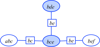
Mixed-inference is even much harder than either max- or sum- inference problems alone: marginal MAP can be NP-hard even on tree structured graphs, as illustrated in the example in Fig. 1 (Koller and Friedman, 2009). The difficulty arises in part because the max and sum operators do not commute, causing the feasible elimination orders to have much higher induced width than for sum- or max-inference. Viewed another way, the marginalization step may destroy the dependency structure of the original graphical model, making the subsequent maximization step far more challenging. Probably for these reasons, there is much less work on marginal MAP than that on joint MAP or marginalization, despite its importance to many practical problems. In practice, it is common to over-use the simpler joint MAP or marginalization even when marginal MAP would be more appropriate. This may cause serious problems, as we illustrate in Example 1 and our empirical results in Section 9.

Contributions. We reformulate the mixed-inference problem to a joint maximization problem as a free energy objective that extends the well-known log-partition function duality form, making it possible to easily extend essentially arbitrary variational algorithms to marginal MAP. In particular, we propose a novel “mixed-product” BP algorithm that is a hybrid of max-product, sum-product, and a special “argmax-product” message updates, as well as a convergent proximal point algorithm that works by iteratively solving pure (or annealed) marginalization tasks. We also present junction graph BP variants of our algorithms, that work on models with higher order cliques. We also discuss mean field methods and highlight their connection to the expectation-maximization (EM) algorithm. We give theoretical guarantees on the global and local optimality of our algorithms for cases when the sum variables form tree structured subgraphs. Our numerical experiments show that our methods can provide significantly better solutions than existing algorithms, including a similar hybrid message passing algorithm by Jiang et al. (2011) and a state-of-the-art algorithm based on local search methods. A preliminary version of this work has appeared in Liu and Ihler (2011b).

Related Work. Expectation-maximization (EM) or variational EM provide one straightforward approach for marginal MAP, by viewing the sum nodes as hidden variables and the max nodes as parameters to be estimated; however, EM is prone to getting stuck at sub-optimal configurations. The classical state-of-the-art approaches include local search methods (e.g., Park and Darwiche, 2004), Markov chain Monte Carlo methods (e.g., Doucet et al., 2002; Yuan et al., 2004), and variational elimination based methods (e.g., Dechter and Rish, 2003; Mauá and de Campos, 2012). Jiang et al. (2011) recently proposed a hybrid message passing algorithm that has a similar form to our mixed-product BP algorithm, but without theoretical guarantees; we show in Section 5.3 that Jiang et al. (2011) can be viewed as an approximation of the marginal MAP problem that exchanges the order of sum and max operators. Another message-passing-style algorithm was proposed very recently in Altarelli et al. (2011) for general multi-stage stochastic optimization problems based on survey propagation, which again does not have optimality guarantees and has a relatively more complicated form. Finally, Ibrahimi et al. (2011) introduces a robust max-product belief propagation for solving a related worst-case robust optimization problem, where the hidden variables are minimized instead of marginalized. To the best of our knowledge, our work is the first general variational framework for marginal MAP, and provides the first strong optimality guarantees.

We begin in Section 2 by introducing background on graphical models and variational inference. We then introduce a novel variational dual representation for marginal MAP in Section 3, and propose analogues of the Bethe and tree-reweighted approximations in Section 4. A class of “mixed-product” message passing algorithms is proposed and analyzed in Section 5 and convergent alternatives are proposed in Section 6 based on proximal point methods. We then discuss the EM algorithm and its connection to our framework in Section 7, and extend our algorithms to junction graphs in Section 8. Finally, we present numerical results in Section 9 and conclude the paper in Section 10.

2 Background

2.1 Graphical Models

Let 𝒙={x1,x2,,xn}𝒙subscript𝑥1subscript𝑥2subscript𝑥𝑛\boldsymbol{x}=\{x_{1},x_{2},\cdots,x_{n}\} be a random vector in a discrete space 𝒳=𝒳1××𝒳n𝒳subscript𝒳1subscript𝒳𝑛\mathcal{X}=\mathcal{X}_{1}\times\cdots\times\mathcal{X}_{n}. Let V={1,,n}𝑉1𝑛V=\{1,\cdots,n\}. For an index set αV𝛼𝑉\alpha\subseteq V, denote by 𝒙αsubscript𝒙𝛼\boldsymbol{x}_{\alpha} the sub-vector {xi:iα}conditional-setsubscript𝑥𝑖𝑖𝛼\{x_{i}\colon i\in\alpha\}, and similarly, 𝒳αsubscript𝒳𝛼\mathcal{X}_{\alpha} the cross product of {𝒳i:iα}conditional-setsubscript𝒳𝑖𝑖𝛼\{\mathcal{X}_{i}\colon i\in\alpha\}. A graphical model defines a factorized probability on 𝒙𝒙\boldsymbol{x},

p(𝒙)=1Z(𝝍)αψα(𝒙α)𝑝𝒙1𝑍𝝍subscriptproduct𝛼subscript𝜓𝛼subscript𝒙𝛼\displaystyle p(\boldsymbol{x})=\frac{1}{Z(\boldsymbol{\psi})}\prod_{\alpha\in\mathcal{I}}\psi_{\alpha}(\boldsymbol{x}_{\alpha})     or p(𝒙;𝜽)=exp[αθα(𝒙α)Φ(𝜽)],𝑝𝒙𝜽subscript𝛼subscript𝜃𝛼subscript𝒙𝛼Φ𝜽\displaystyle p(\boldsymbol{x};\boldsymbol{\theta})=\exp[\sum_{\alpha\in\mathcal{I}}\theta_{\alpha}(\boldsymbol{x}_{\alpha})-\Phi(\boldsymbol{\theta})], (1)

where \mathcal{I} is a set of subsets of variable indexes, ψα:𝒳α+:subscript𝜓𝛼subscript𝒳𝛼superscript\psi_{\alpha}\colon\mathcal{X}_{\alpha}\to\mathbb{R}^{+} is called a factor function, and θα(𝒙α)=logψα(𝒙α)subscript𝜃𝛼subscript𝒙𝛼subscript𝜓𝛼subscript𝒙𝛼\theta_{\alpha}(\boldsymbol{x}_{\alpha})=\log\psi_{\alpha}(\boldsymbol{x}_{\alpha}). Since the xisubscript𝑥𝑖x_{i} are discrete, the functions ψ𝜓\psi and θ𝜃\theta are tables; by alternatively viewing θ𝜃\theta as a vector, it is interpreted as the natural parameter in an overcomplete, exponential family representation. Let 𝝍𝝍\boldsymbol{\psi} and 𝜽𝜽\boldsymbol{\theta} be the joint vector of all ψαsubscript𝜓𝛼\psi_{\alpha} and θαsubscript𝜃𝛼\theta_{\alpha} respectively, e.g., 𝜽={θα(𝒙α):αI,𝒙α𝒳α}𝜽conditional-setsubscript𝜃𝛼subscript𝒙𝛼formulae-sequence𝛼𝐼subscript𝒙𝛼subscript𝒳𝛼\boldsymbol{\theta}=\{\theta_{\alpha}(\boldsymbol{x}_{\alpha})\colon\alpha\in I,\boldsymbol{x}_{\alpha}\in\mathcal{X}_{\alpha}\}. The normalization constant Z(𝝍)𝑍𝝍Z(\boldsymbol{\psi}), called partition function, normalizes the probability to sum to one, and Φ(𝜽):=logZ(𝝍)\Phi(\boldsymbol{\theta})\mathrel{\mathop{:}}=\log Z(\boldsymbol{\psi}) is called the log-partition function,

Φ(𝜽)=log𝒙𝒳exp[θ(𝒙)],Φ𝜽subscript𝒙𝒳𝜃𝒙\displaystyle\Phi(\boldsymbol{\theta})=\log\sum_{\boldsymbol{x}\in\mathcal{X}}\exp[\theta(\boldsymbol{x})],

where we define θ(𝒙)=αθα(𝒙α)𝜃𝒙subscript𝛼subscript𝜃𝛼subscript𝒙𝛼\theta(\boldsymbol{x})=\sum_{\alpha\in\mathcal{I}}\theta_{\alpha}(\boldsymbol{x}_{\alpha}) to be the joint potential function that maps from 𝒳𝒳\mathcal{X} to \mathbb{R}. The factorization structure of p(𝒙)𝑝𝒙p(\boldsymbol{x}) can be represented by an undirected graph G=(V,E)𝐺𝑉𝐸G=(V,E), where each node iV𝑖𝑉i\in V maps to a variable xisubscript𝑥𝑖x_{i}, and each edge (ij)E𝑖𝑗𝐸(ij)\in E corresponds to two variables xisubscript𝑥𝑖x_{i} and xjsubscript𝑥𝑗x_{j} that coappear in some factor function ψαsubscript𝜓𝛼\psi_{\alpha}, that is, {i,j}α𝑖𝑗𝛼\{i,j\}\subseteq\alpha. The set \mathcal{I} is then a set of cliques (fully connected subgraphs) of G𝐺G. For the purpose of illustration, we mainly restrict our scope on the set of pairwise models, on which \mathcal{I} is the set of nodes and edges, i.e., =EV𝐸𝑉\mathcal{I}=E\cup V. However, we show how to extend our algorithms to models with higher order cliques in Section 8.

2.2 Sum-Inference Problems and Variational Approximation

Sum-inference is the task of marginalizing (summing out) variables in the model, e.g., calculating the marginal probabilities of single variables, or the normalization constant Z𝑍Z,

p(xi)=𝒙V{i}exp[θ(𝒙)Φ(𝜽)],𝑝subscript𝑥𝑖subscriptsubscript𝒙𝑉𝑖𝜃𝒙Φ𝜽\displaystyle p(x_{i})=\sum_{\boldsymbol{x}_{V\setminus\{i\}}}\exp[\theta(\boldsymbol{x})-\Phi(\boldsymbol{\theta})], Φ(𝜽)=log𝒙exp[θ(𝒙)].Φ𝜽subscript𝒙𝜃𝒙\displaystyle\Phi(\boldsymbol{\theta})=\log\sum_{\boldsymbol{x}}\exp[\theta(\boldsymbol{x})]. (2)

Unfortunately, the problem is generally #P-complete, and the straightforward calculation requires summing over an exponential number of terms. Variational methods are a class of approximation algorithms that transform the marginalization problem into a continuous optimization problem, which is then typically solved approximately.

Marginal Polytope. The marginal polytope is a key concept in variational inference. We define the marginal polytope 𝕄𝕄\mathbb{M} to be the set of local marginal probabilities 𝝉={τα(𝒙α):α}𝝉conditional-setsubscript𝜏𝛼subscript𝒙𝛼𝛼{\boldsymbol{\tau}}=\{\tau_{\alpha}(\boldsymbol{x}_{\alpha})\colon\alpha\in\mathcal{I}\} that are extensible to a valid joint distribution, i.e.,

𝕄={𝝉: joint distribution q(𝒙), s.t. τα(𝒙α)=𝒙Vαq(𝒙) for α}.𝕄conditional-set𝝉 joint distribution q(𝒙), s.t. τα(𝒙α)=𝒙Vαq(𝒙) for α\mathbb{M}=\{{\boldsymbol{\tau}}\ :\ \text{$\exists$ joint distribution $q(\boldsymbol{x})$, s.t. $\tau_{\alpha}(\boldsymbol{x}_{\alpha})=\sum_{\boldsymbol{x}_{V\setminus\alpha}}q(\boldsymbol{x})$ for $\forall\alpha\in\mathcal{I}$}\}. (3)

Denote by 𝒬[𝝉]𝒬delimited-[]𝝉\mathcal{Q}[{\boldsymbol{\tau}}] the set of joint distributions whose marginals are consistent with 𝝉𝕄𝝉𝕄{\boldsymbol{\tau}}\in\mathbb{M}; by the principle of maximum entropy (Jaynes, 1957), there exists a unique distribution in 𝒬[𝝉]𝒬delimited-[]𝝉\mathcal{Q}[{\boldsymbol{\tau}}] that has maximum entropy and follows the exponential family form for some 𝜽𝜽\boldsymbol{\theta}.222In the case that p(𝒙)𝑝𝒙p(\boldsymbol{x}) has zero elements, the maximum entropy distribution is still unique and satisfies the exponential family form, but the corresponding 𝜽𝜽\boldsymbol{\theta} has negative infinite values (Jaynes, 1957). With an abuse of notation, we denote these unique global distributions by τ(𝒙)𝜏𝒙\tau(\boldsymbol{x}), and we do not distinguish τ(𝒙)𝜏𝒙\tau(\boldsymbol{x}) and 𝝉𝝉{\boldsymbol{\tau}} when it is clear from the context.

Log-partition Function Duality. A key result to many variational methods is that the log-partition function Φ(𝜽)Φ𝜽\Phi(\boldsymbol{\theta}) is a convex function of 𝜽𝜽\boldsymbol{\theta} and can be rewritten into a convex dual form,

Φ(𝜽)=max𝝉𝕄{𝜽,𝝉+H(𝝉)},Φ𝜽subscript𝝉𝕄𝜽𝝉𝐻𝝉\displaystyle\Phi(\boldsymbol{\theta})=\max_{{\boldsymbol{\tau}}\in\mathbb{M}}\big{\{}\langle\boldsymbol{\theta},{\boldsymbol{\tau}}\rangle+H({\boldsymbol{\tau}})\big{\}}, (4)

where 𝜽,𝝉=α𝒙αθα(𝒙α)τα(𝒙α)𝜽𝝉subscript𝛼subscriptsubscript𝒙𝛼subscript𝜃𝛼subscript𝒙𝛼subscript𝜏𝛼subscript𝒙𝛼\langle\boldsymbol{\theta},{\boldsymbol{\tau}}\rangle=\sum_{\alpha}\sum_{\boldsymbol{x}_{\alpha}}\theta_{\alpha}(\boldsymbol{x}_{\alpha})\tau_{\alpha}(\boldsymbol{x}_{\alpha}) is the vectorized inner product, and H(𝝉)𝐻𝝉H({\boldsymbol{\tau}}) is the entropy of the corresponding global distribution τ(𝒙)𝜏𝒙\tau(\boldsymbol{x}), i.e., H(𝝉)=𝒙τ(𝒙)logτ(𝒙)𝐻𝝉subscript𝒙𝜏𝒙𝜏𝒙H({\boldsymbol{\tau}})=-\sum_{\boldsymbol{x}}\tau(\boldsymbol{x})\log\tau(\boldsymbol{x}). The unique maximum 𝝉superscript𝝉{\boldsymbol{\tau}}^{*} of (4) exactly equals the marginals of the original distribution p(𝒙;𝜽)𝑝𝒙𝜽p(\boldsymbol{x};\boldsymbol{\theta}), that is, τ(𝒙)=p(𝒙;𝜽)superscript𝜏𝒙𝑝𝒙𝜽\tau^{*}(\boldsymbol{x})=p(\boldsymbol{x};\boldsymbol{\theta}). We call Fsum(𝝉,𝜽)=𝜽,𝝉+H(𝝉)subscript𝐹𝑠𝑢𝑚𝝉𝜽𝜽𝝉𝐻𝝉F_{sum}({\boldsymbol{\tau}},\boldsymbol{\theta})=\langle\boldsymbol{\theta},{\boldsymbol{\tau}}\rangle+H({\boldsymbol{\tau}}) the sum-inference free energy (although technically the negative free energy).

The dual form (4) transforms the marginalization problem into a continuous optimization, but does not make it any easier: the marginal polytope 𝕄𝕄\mathbb{M} is defined by an exponential number of linear constraints, and the entropy term in the objective function is as difficult to calculate as the log-partition function. However, (4) provides a framework for deriving efficient approximate inference algorithms by approximating both the marginal polytope and the entropy (Wainwright and Jordan, 2008).

BP-like Methods. Many approximation methods replace 𝕄𝕄\mathbb{M} with the locally consistent polytope 𝕃𝕃\mathbb{L}; in pairwise models, it is the set of singleton and pairwise “pseduo-marginals” {τi(xi):iV}conditional-setsubscript𝜏𝑖subscript𝑥𝑖𝑖𝑉\{\tau_{i}(x_{i})\colon i\in V\} and {τij(xi,xj):(ij)E}conditional-setsubscript𝜏𝑖𝑗subscript𝑥𝑖subscript𝑥𝑗𝑖𝑗𝐸\{\tau_{ij}(x_{i},x_{j})\colon(ij)\in E\} that are consistent on their intersections, i.e.,

𝕃={τi,τij:xiτij(xi,xj)=τj(xj),xiτi(xi)=1,τij(xi,xj)0}.𝕃conditional-setsubscript𝜏𝑖subscript𝜏𝑖𝑗formulae-sequencesubscriptsubscript𝑥𝑖subscript𝜏𝑖𝑗subscript𝑥𝑖subscript𝑥𝑗subscript𝜏𝑗subscript𝑥𝑗formulae-sequencesubscriptsubscript𝑥𝑖subscript𝜏𝑖subscript𝑥𝑖1subscript𝜏𝑖𝑗subscript𝑥𝑖subscript𝑥𝑗0\mathbb{L}=\{\tau_{i},\tau_{ij}~{}\colon~{}\sum_{x_{i}}\tau_{ij}(x_{i},x_{j})=\tau_{j}(x_{j}),~{}\sum_{x_{i}}\tau_{i}(x_{i})=1,~{}\tau_{ij}(x_{i},x_{j})\geq 0\}. (5)

Since not all such pseudo-marginals have valid global distributions, it is easy to see that 𝕃𝕃\mathbb{L} is an outer bound of 𝕄𝕄\mathbb{M}, that is, 𝕄𝕃𝕄𝕃\mathbb{M}\subseteq\mathbb{L}. Note that this means there may not exist a global distribution τ(𝒙)𝜏𝒙\tau(\boldsymbol{x}) for 𝝉𝝉{\boldsymbol{\tau}} in 𝕃𝕃\mathbb{L}.

The free energy remains intractable (and is not even well-defined) in 𝕃𝕃\mathbb{L}. We typically approximate the free energy by a combination of singleton and pairwise entropies, which only requires knowing τisubscript𝜏𝑖\tau_{i} and τijsubscript𝜏𝑖𝑗\tau_{ij}. For example, the Bethe free energy approximation (Yedidia et al., 2003) is

H(𝝉)iVHi(𝝉)(ij)EIij(𝝉),𝐻𝝉subscript𝑖𝑉subscript𝐻𝑖𝝉subscript𝑖𝑗𝐸subscript𝐼𝑖𝑗𝝉\displaystyle H({\boldsymbol{\tau}})\approx\sum_{i\in V}H_{{i}}({\boldsymbol{\tau}})-\sum_{(ij)\in E}I_{{ij}}({\boldsymbol{\tau}}), Φ(𝜽)max𝝉𝕃{𝜽,𝝉+iVHi(𝝉)(ij)EIij(𝝉)},Φ𝜽subscript𝝉𝕃𝜽𝝉subscript𝑖𝑉subscript𝐻𝑖𝝉subscript𝑖𝑗𝐸subscript𝐼𝑖𝑗𝝉\displaystyle\Phi(\boldsymbol{\theta})\approx\max_{{\boldsymbol{\tau}}\in\mathbb{L}}\big{\{}\langle\boldsymbol{\theta},{\boldsymbol{\tau}}\rangle+\sum_{i\in V}H_{{i}}({\boldsymbol{\tau}})-\sum_{(ij)\in E}I_{{ij}}({\boldsymbol{\tau}})\big{\}}, (6)

where Hi(𝝉)subscript𝐻𝑖𝝉H_{{i}}({\boldsymbol{\tau}}) is the entropy of τi(xi)subscript𝜏𝑖subscript𝑥𝑖\tau_{i}(x_{i}) and Iij(𝝉)subscript𝐼𝑖𝑗𝝉I_{{ij}}({\boldsymbol{\tau}}) the mutual information of xisubscript𝑥𝑖x_{i} and xjsubscript𝑥𝑗x_{j}, i.e.,

Hi(𝝉)=xiτi(xi)logτi(xi),subscript𝐻𝑖𝝉subscriptsubscript𝑥𝑖subscript𝜏𝑖subscript𝑥𝑖subscript𝜏𝑖subscript𝑥𝑖\displaystyle H_{{i}}({\boldsymbol{\tau}})=-\sum_{x_{i}}\tau_{i}(x_{i})\log\tau_{i}(x_{i}), Iij(𝝉)=xi,xjτij(xi,xj)logτij(xi,xj)τi(xi)τj(xj).subscript𝐼𝑖𝑗𝝉subscriptsubscript𝑥𝑖subscript𝑥𝑗subscript𝜏𝑖𝑗subscript𝑥𝑖subscript𝑥𝑗subscript𝜏𝑖𝑗subscript𝑥𝑖subscript𝑥𝑗subscript𝜏𝑖subscript𝑥𝑖subscript𝜏𝑗subscript𝑥𝑗\displaystyle I_{{ij}}({\boldsymbol{\tau}})=\sum_{x_{i},x_{j}}\tau_{ij}(x_{i},x_{j})\log\frac{\tau_{ij}(x_{i},x_{j})}{\tau_{i}(x_{i})\tau_{j}(x_{j})}.

We sometimes abbreviate Hi(𝝉)subscript𝐻𝑖𝝉H_{{i}}({\boldsymbol{\tau}}) and Iij(𝝉)subscript𝐼𝑖𝑗𝝉I_{{ij}}({\boldsymbol{\tau}}) into Hisubscript𝐻𝑖H_{i} and Iijsubscript𝐼𝑖𝑗I_{ij} for convenience. The well-known loopy belief propagation (BP) algorithm of Pearl (1988) can be interpreted as a fixed point algorithm to optimize the Bethe free energy in (6) on the locally consistent polytope 𝕃𝕃\mathbb{L} (Yedidia et al., 2003). Unfortunately, the Bethe free energy is a non-concave function of 𝝉𝝉{\boldsymbol{\tau}}, causing (6) to be a non-convex optimization. The tree reweighted (TRW) free energy is a convex surrogate of the Bethe free energy (Wainwright et al., 2005a),

Φ(𝜽)max𝝉𝕃{𝜽,𝝉+iVHi(𝝉)(ij)EρijIij(𝝉)},Φ𝜽subscript𝝉𝕃𝜽𝝉subscript𝑖𝑉subscript𝐻𝑖𝝉subscript𝑖𝑗𝐸subscript𝜌𝑖𝑗subscript𝐼𝑖𝑗𝝉\displaystyle\Phi(\boldsymbol{\theta})\approx\max_{{\boldsymbol{\tau}}\in\mathbb{L}}\big{\{}\langle\boldsymbol{\theta},{\boldsymbol{\tau}}\rangle+\sum_{i\in V}H_{{i}}({\boldsymbol{\tau}})-\sum_{(ij)\in E}\rho_{ij}I_{{ij}}({\boldsymbol{\tau}})\big{\}}, (7)

where {ρij:(ij)E}conditional-setsubscript𝜌𝑖𝑗𝑖𝑗𝐸\{\rho_{ij}\colon(ij)\in E\} is a set of positive edge appearance probabilities obtained from a weighted collection of spanning trees of G𝐺G (see Wainwright et al. (2005a) and Section 4.2 for the detailed definition). The TRW approximation in (7) is a convex optimization problem, and is guaranteed to give an upper bound of the true log-partition function. A message passing algorithm similar to loopy BP, called tree reweighted BP, can be derived as a fixed point algorithm for solving the convex optimization in (7).

Mean-field-based Methods. Mean-field-based methods are another set of approximate inference algorithms, which work by restricting 𝕄𝕄\mathbb{M} to a set of tractable distributions, on which both the marginal polytope and the joint entropy are tractable. Precisely, let 𝕄mfsubscript𝕄𝑚𝑓\mathbb{M}_{mf} be a subset of 𝕄𝕄\mathbb{M} that corresponds to a set of tractable distributions, e.g., the set of fully factored distributions, 𝕄mf={𝝉𝕄:τ(𝒙)=iVτi(xi)}subscript𝕄𝑚𝑓conditional-set𝝉𝕄𝜏𝒙subscriptproduct𝑖𝑉subscript𝜏𝑖subscript𝑥𝑖\mathbb{M}_{mf}=\{{\boldsymbol{\tau}}\in\mathbb{M}\colon\tau(\boldsymbol{x})=\prod_{i\in V}\tau_{i}(x_{i})\}. Note that the joint entropy H(𝝉)𝐻𝝉H({\boldsymbol{\tau}}) for any 𝝉𝕄mf𝝉subscript𝕄𝑚𝑓{\boldsymbol{\tau}}\in\mathbb{M}_{mf} decomposes to the sum of singleton entropies Hi(𝝉)subscript𝐻𝑖𝝉H_{{i}}({\boldsymbol{\tau}}) of the marginal distributions τi(xi)subscript𝜏𝑖subscript𝑥𝑖\tau_{i}(x_{i}). This method then approximates the log-partition function (4) by

max𝝉𝕄mf{𝜽,𝝉+iVHi(𝝉)},subscript𝝉subscript𝕄𝑚𝑓𝜽𝝉subscript𝑖𝑉subscript𝐻𝑖𝝉\displaystyle\max_{{\boldsymbol{\tau}}\in\mathbb{M}_{mf}}\big{\{}\langle\boldsymbol{\theta},{\boldsymbol{\tau}}\rangle+\sum_{i\in V}H_{{i}}({\boldsymbol{\tau}})\big{\}}, (8)

which is guaranteed to give a lower bound of the log-partition function. Unfortunately, mean field methods usually lead to non-convex optimization problems, because 𝕄mfsubscript𝕄𝑚𝑓\mathbb{M}_{mf} is often a non-convex set. In practice, block coordinate descent methods can be adopted to find the local optima of (8).

2.3 Max-Inference Problems

Combinatorial maximization (max-inference), or maximum a posteriori (MAP), problems are the tasks of finding a mode of the joint probability. That is,

Φ(𝜽)=max𝒙θ(𝒙),𝒙=argmax𝒙θ(𝒙),formulae-sequencesubscriptΦ𝜽subscript𝒙𝜃𝒙superscript𝒙subscriptargmax𝒙𝜃𝒙\displaystyle\Phi_{\infty}(\boldsymbol{\theta})=\max_{\boldsymbol{x}}\theta(\boldsymbol{x}),~{}~{}~{}~{}~{}~{}~{}~{}~{}~{}~{}\boldsymbol{x}^{*}=\operatorname*{arg\,max}_{\boldsymbol{x}}\theta(\boldsymbol{x}), (9)

where 𝒙superscript𝒙\boldsymbol{x}^{*} is a MAP configuration and Φ(𝜽)subscriptΦ𝜽\Phi_{\infty}(\boldsymbol{\theta}) the optimal energy value. This problem can be reformed into a linear program,

Φ(𝜽)=max𝝉𝕄𝜽,𝝉,subscriptΦ𝜽subscript𝝉𝕄𝜽𝝉\Phi_{\infty}(\boldsymbol{\theta})=\max_{{\boldsymbol{\tau}}\in\mathbb{M}}\langle\boldsymbol{\theta},{\boldsymbol{\tau}}\rangle, (10)

which attains its maximum when τ(𝒙)=𝟏(𝒙=𝒙)superscript𝜏𝒙1𝒙superscript𝒙\tau^{*}(\boldsymbol{x})=\boldsymbol{1}(\boldsymbol{x}=\boldsymbol{x}^{*}), where 𝟏()1\boldsymbol{1}(\cdot) is the Kronecker delta function, defined as 𝟏(t)=11𝑡1\boldsymbol{1}(t)=1 if condition t𝑡t is true, and zero otherwise. If there are multiple MAP solutions, say {𝒙k:k=1,,K}conditional-setsuperscript𝒙absent𝑘𝑘1𝐾\{\boldsymbol{x}^{*k}\colon k=1,\ldots,K\}, then any convex combination kck𝟏(𝒙=𝒙k)subscript𝑘subscript𝑐𝑘1𝒙superscript𝒙absent𝑘\sum_{k}c_{k}\boldsymbol{1}(\boldsymbol{x}=\boldsymbol{x}^{*k}) with kck=1,ci0formulae-sequencesubscript𝑘subscript𝑐𝑘1subscript𝑐𝑖0\sum_{k}c_{k}=1,c_{i}\geq 0 leads to a maximum of (10).

The problem in (10) remains NP-hard, because the marginal polytope 𝕄𝕄\mathbb{M} includes exponentially many inequality constraints. Most variational methods for MAP (e.g., Wainwright et al., 2005b; Werner, 2007) can be interpreted as relaxing 𝕄𝕄\mathbb{M} to the locally consistent polytop 𝕃𝕃\mathbb{L}, yielding a linear relaxation of the original integer programming problem. Note that (10) differs from (4) only by its lack of an entropy term; in the next section, we generalize this similarity to marginal MAP.

2.4 Marginal MAP Problems

Marginal MAP is simply a hybrid of the max- and sum- inference tasks. Let A𝐴A be a subset of nodes V𝑉V, and B=V\A𝐵\𝑉𝐴B=V\backslash A be the complement of A𝐴A. The marginal MAP problem seeks a partial configuration 𝒙Bsuperscriptsubscript𝒙𝐵\boldsymbol{x}_{B}^{*} that has the maximum marginal probability p(𝒙B)=𝒙Ap(𝒙)𝑝subscript𝒙𝐵subscriptsubscript𝒙𝐴𝑝𝒙p(\boldsymbol{x}_{B})=\sum_{\boldsymbol{x}_{A}}p(\boldsymbol{x}), where A𝐴A is the set of sum nodes to be marginalized out, and B𝐵B the max nodes to be optimized. We call this a type of “mixed-inference” problem, since it involves more than one type of variable elimination operator. To facilitate developing our duality results, we formulate marginal MAP in terms of the exponential family representation,

ΦAB(𝜽)=max𝒙BQ(𝒙B;𝜽),subscriptΦ𝐴𝐵𝜽subscriptsubscript𝒙𝐵𝑄subscript𝒙𝐵𝜽\displaystyle\Phi_{AB}(\boldsymbol{\theta})=\max_{\boldsymbol{x}_{B}}Q(\boldsymbol{x}_{B};\boldsymbol{\theta}), where Q(𝒙B;𝜽)=log𝒙Aexp[θ(𝒙)],where 𝑄subscript𝒙𝐵𝜽subscriptsubscript𝒙𝐴𝜃𝒙\displaystyle\text{where~{}~{}~{}}Q(\boldsymbol{x}_{B};\boldsymbol{\theta})=\log\sum_{\boldsymbol{x}_{A}}\exp[\theta(\boldsymbol{x})], (11)

where the maximum point 𝒙Bsuperscriptsubscript𝒙𝐵\boldsymbol{x}_{B}^{*} of Q(𝒙B;𝜽)𝑄subscript𝒙𝐵𝜽Q(\boldsymbol{x}_{B};\boldsymbol{\theta}) is the marginal MAP solution.

max:𝒙Bsubscript𝒙𝐵\boldsymbol{x}_{B}sum:𝒙Asubscript𝒙𝐴\boldsymbol{x}_{A}Marginal MAP:𝒙B=argmax𝒙Bp(𝒙B)superscriptsubscript𝒙𝐵subscriptargmaxsubscript𝒙𝐵𝑝subscript𝒙𝐵\displaystyle\boldsymbol{x}_{B}^{*}=\operatorname*{arg\,max}_{\boldsymbol{x}_{B}}p(\boldsymbol{x}_{B})=argmax𝒙B𝒙Ap(𝒙)absentsubscriptargmaxsubscript𝒙𝐵subscriptsubscript𝒙𝐴𝑝𝒙\displaystyle\ \ =\operatorname*{arg\,max}_{\boldsymbol{x}_{B}}\sum_{\boldsymbol{x}_{A}}p(\boldsymbol{x}).
Refer to caption
Figure 1: An example from Koller and Friedman (2009) in which a marginal MAP query on a tree requires exponential time complexity. The marginalization over 𝒙Asubscript𝒙𝐴\boldsymbol{x}_{A} destroys the conditional dependency structure in the marginal distribution p(𝒙B)𝑝subscript𝒙𝐵p(\boldsymbol{x}_{B}), causing an intractable maximization problem over 𝒙Bsubscript𝒙𝐵\boldsymbol{x}_{B}. The exact variable elimination method, which sequentially marginalizes the sum nodes and then maximizes the max nodes, has time complexity of O(exp(n))𝑂𝑛O(\exp(n)), where n𝑛n is the length of the chain.

Although similar to max- and sum-inference, marginal MAP is significantly harder than either of them. A classic example is shown in Fig. 1, where marginal MAP is NP-hard even on a tree structured graph (Koller and Friedman, 2009). The main difficulty arises because the max and sum operators do not commute, which restricts feasible elimination orders to those with all the sum nodes eliminated before any max nodes. In the worst case, marginalizing the sum nodes 𝒙Asubscript𝒙𝐴\boldsymbol{x}_{A} may destroy any conditional independence among the max nodes 𝒙Bsubscript𝒙𝐵\boldsymbol{x}_{B}, making it difficult to represent or optimize Q(𝒙B;θ)𝑄subscript𝒙𝐵𝜃Q(\boldsymbol{x}_{B};\theta), even when the sum part alone is tractable (such as when the nodes in A𝐴A form a tree).

Despite its computational difficulty, marginal MAP plays an essential role in many practical scenarios. The marginal MAP configuration 𝒙Bsuperscriptsubscript𝒙𝐵\boldsymbol{x}_{B}^{*} in (11) is Bayes optimal in the sense that it minimizes the expected error on B𝐵B, 𝔼[𝟏(𝒙B=𝒙B)]𝔼delimited-[]1superscriptsubscript𝒙𝐵subscript𝒙𝐵\mathbb{E}[\boldsymbol{1}(\boldsymbol{x}_{B}^{*}=\boldsymbol{x}_{B})], where 𝔼[]𝔼delimited-[]\mathbb{E}[\cdot] denotes the expectation under distribution p(𝒙;𝜽)𝑝𝒙𝜽p(\boldsymbol{x};\boldsymbol{\theta}). Here, the variables 𝒙Asubscript𝒙𝐴\boldsymbol{x}_{A} are not included in the error criterion, for example because they are “nuisance” hidden variables of no direct interest, or unobserved or inaccurately measured model parameters. In contrast, the joint MAP configuration 𝒙superscript𝒙\boldsymbol{x}^{*} minimizes the joint error 𝔼[𝟏(𝒙=𝒙)]𝔼delimited-[]1superscript𝒙𝒙\mathbb{E}[\boldsymbol{1}(\boldsymbol{x}^{*}=\boldsymbol{x})], but gives no guarantees on the partial error 𝔼[𝟏(𝒙B=𝒙B)]𝔼delimited-[]1superscriptsubscript𝒙𝐵subscript𝒙𝐵\mathbb{E}[\boldsymbol{1}(\boldsymbol{x}_{B}^{*}=\boldsymbol{x}_{B})]. In practice, perhaps because of the wide availability of efficient algorithms for joint MAP, researchers tend to over-use joint MAP even in cases where marginal MAP would be more appropriate. The following toy example shows that this seemingly reasonable approach can sometimes cause serious problems.

Example 1 (Weather Dilemma).

Denote by xb{𝚛𝚊𝚒𝚗𝚢,𝚜𝚞𝚗𝚗𝚢}subscript𝑥𝑏𝚛𝚊𝚒𝚗𝚢𝚜𝚞𝚗𝚗𝚢x_{b}\in\{{\tt{\tt rainy}},{\tt{\tt sunny}}\} the weather condition of Irvine, and xa{𝚠𝚊𝚕𝚔,𝚍𝚛𝚒𝚟𝚎}subscript𝑥𝑎𝚠𝚊𝚕𝚔𝚍𝚛𝚒𝚟𝚎x_{a}\in\{{\tt walk},{\tt drive}\} whether Alice drives or walks to the school depending on the weather condition. Assume the probabilities of xbsubscript𝑥𝑏x_{b} and xasubscript𝑥𝑎x_{a} are
p(xb)::𝑝subscript𝑥𝑏absentp(x_{b}): rainy 0.40.40.4 sunny 0.60.60.6 p(xa|xb)::𝑝conditionalsubscript𝑥𝑎subscript𝑥𝑏absentp(x_{a}|x_{b}): walk drive rainy 1/8181/8 7/8787/8 sunny 1/2121/2 1/2121/2
The task is to calculate the most likely weather condition of Irvine, which is obviously
sunny according to p(xb)𝑝subscript𝑥𝑏p(x_{b}). The marginal MAP, xb=argmaxxbp(xb)=𝚜𝚞𝚗𝚗𝚢superscriptsubscript𝑥𝑏subscriptargmaxsubscript𝑥𝑏𝑝subscript𝑥𝑏𝚜𝚞𝚗𝚗𝚢x_{b}^{*}=\operatorname*{arg\,max}_{x_{b}}p(x_{b})={\tt sunny}, gives the correct answer. However, the full MAP estimator, [xa,xb]=argmaxp(xa,xb)=[𝚍𝚛𝚒𝚟𝚎,𝚛𝚊𝚒𝚗𝚢]superscriptsubscript𝑥𝑎superscriptsubscript𝑥𝑏argmax𝑝subscript𝑥𝑎subscript𝑥𝑏𝚍𝚛𝚒𝚟𝚎𝚛𝚊𝚒𝚗𝚢[x_{a}^{*},x_{b}^{*}]=\operatorname*{arg\,max}p(x_{a},x_{b})=[{\tt drive},{\tt rainy}], gives answer xb=𝚛𝚊𝚒𝚗𝚢superscriptsubscript𝑥𝑏𝚛𝚊𝚒𝚗𝚢x_{b}^{*}={\tt rainy} (by dropping the xasuperscriptsubscript𝑥𝑎x_{a}^{*} component), which is obviously wrong. Paradoxically, if p(xa|xb)𝑝conditionalsubscript𝑥𝑎subscript𝑥𝑏p(x_{a}|x_{b}) is changed (say, corresponding to a different person), the solution returned by full MAP could be different.

In the above example, since no evidence on xasubscript𝑥𝑎x_{a} is observed, the conditional probability p(xa|xb)𝑝conditionalsubscript𝑥𝑎subscript𝑥𝑏p(x_{a}|x_{b}) does not provide useful information for xbsubscript𝑥𝑏x_{b}, but instead provides misleading information when it is incorporated in the full MAP estimator. The marginal MAP, on the other hand, eliminates the influence of the irrelevant p(xa|xb)𝑝conditionalsubscript𝑥𝑎subscript𝑥𝑏p(x_{a}|x_{b}) by marginalizing (or averaging) xasubscript𝑥𝑎x_{a}. In general, the marginal MAP and full MAP can differ significantly when the uncertainty in the hidden variables changes as a function of 𝒙Bsubscript𝒙𝐵\boldsymbol{x}_{B}.

3 A Dual Representation for Marginal MAP

In this section, we present our main result, a dual representation of the marginal MAP problem (11). Our dual representation generalizes that of sum-inference in (4) and max-inference in (10), and provides a unified framework for solving marginal MAP problems.

Theorem 2.

The marginal MAP energy ΦAB(𝛉)subscriptΦ𝐴𝐵𝛉\Phi_{AB}(\boldsymbol{\theta}) in (11) has a dual representation,

ΦAB(𝜽)=max𝝉𝕄{𝜽,𝝉+HA|B(𝝉)},subscriptΦ𝐴𝐵𝜽subscript𝝉𝕄𝜽𝝉subscript𝐻conditional𝐴𝐵𝝉\Phi_{AB}(\boldsymbol{\theta})=\max_{{\boldsymbol{\tau}}\in\mathbb{M}}\{\langle\boldsymbol{\theta},{\boldsymbol{\tau}}\rangle+H_{A|B}({\boldsymbol{\tau}})\}, (12)

where HA|B(𝛕)subscript𝐻conditional𝐴𝐵𝛕H_{A|B}({\boldsymbol{\tau}}) is a conditional entropy, HA|B(𝛕)=𝐱τ(𝐱)logτ(𝐱A|𝐱B)subscript𝐻conditional𝐴𝐵𝛕subscript𝐱𝜏𝐱𝜏conditionalsubscript𝐱𝐴subscript𝐱𝐵H_{A|B}({\boldsymbol{\tau}})=-\sum_{\boldsymbol{x}}\tau(\boldsymbol{x})\log\tau(\boldsymbol{x}_{A}|\boldsymbol{x}_{B}). If Q(𝐱B;𝛉)𝑄subscript𝐱𝐵𝛉Q(\boldsymbol{x}_{B};\boldsymbol{\theta}) has a unique maximum 𝐱Bsuperscriptsubscript𝐱𝐵\boldsymbol{x}_{B}^{*}, the maximum point 𝛕superscript𝛕{\boldsymbol{\tau}}^{*} of (12) is also unique, satisfying τ(𝐱)=τ(𝐱B)τ(𝐱A|𝐱B)superscript𝜏𝐱superscript𝜏subscript𝐱𝐵superscript𝜏conditionalsubscript𝐱𝐴subscript𝐱𝐵\tau^{*}(\boldsymbol{x})=\tau^{*}(\boldsymbol{x}_{B})\tau^{*}(\boldsymbol{x}_{A}|\boldsymbol{x}_{B}), where τ(𝐱B)=𝟏(𝐱B=𝐱B)superscript𝜏subscript𝐱𝐵1subscript𝐱𝐵superscriptsubscript𝐱𝐵\tau^{*}(\boldsymbol{x}_{B})=\boldsymbol{1}(\boldsymbol{x}_{B}=\boldsymbol{x}_{B}^{*}) and τ(𝐱A|𝐱B)=p(𝐱A|𝐱B;𝛉)superscript𝜏conditionalsubscript𝐱𝐴subscript𝐱𝐵𝑝conditionalsubscript𝐱𝐴subscript𝐱𝐵𝛉\tau^{*}(\boldsymbol{x}_{A}|\boldsymbol{x}_{B})=p(\boldsymbol{x}_{A}|\boldsymbol{x}_{B};\boldsymbol{\theta}) 333Since τ(𝐱B)=0𝜏subscript𝐱𝐵0\tau(\boldsymbol{x}_{B})=0 if 𝐱B𝐱Bsubscript𝐱𝐵superscriptsubscript𝐱𝐵\boldsymbol{x}_{B}\neq\boldsymbol{x}_{B}^{*}, we do not necessarily need to define τ(𝐱A|𝐱B)superscript𝜏conditionalsubscript𝐱𝐴subscript𝐱𝐵\tau^{*}(\boldsymbol{x}_{A}|\boldsymbol{x}_{B}) for 𝐱B𝐱Bsubscript𝐱𝐵superscriptsubscript𝐱𝐵\boldsymbol{x}_{B}\neq\boldsymbol{x}_{B}^{*}..

Proof.

For any 𝝉𝕄𝝉𝕄{\boldsymbol{\tau}}\in\mathbb{M} and its corresponding global distribution τ(𝒙)𝜏𝒙\tau(\boldsymbol{x}), consider the conditional KL divergence between τ(𝒙A|𝒙B)𝜏conditionalsubscript𝒙𝐴subscript𝒙𝐵\tau(\boldsymbol{x}_{A}|\boldsymbol{x}_{B}) and p(𝒙A|𝒙B;𝜽)𝑝conditionalsubscript𝒙𝐴subscript𝒙𝐵𝜽p(\boldsymbol{x}_{A}|\boldsymbol{x}_{B};\boldsymbol{\theta}),

DKL[τ(𝒙A|𝒙B)||p(𝒙A|𝒙B;𝜽)]=𝒙τ(𝒙)logτ(𝒙A|𝒙B)p(𝒙A|𝒙B;𝜽)\displaystyle D_{\mathrm{KL}}[\tau(\boldsymbol{x}_{A}|\boldsymbol{x}_{B})||p(\boldsymbol{x}_{A}|\boldsymbol{x}_{B};\boldsymbol{\theta})]=\sum_{\boldsymbol{x}}\tau(\boldsymbol{x})\log\frac{\tau(\boldsymbol{x}_{A}|\boldsymbol{x}_{B})}{p(\boldsymbol{x}_{A}|\boldsymbol{x}_{B};\boldsymbol{\theta})}
=HA|B(𝝉)𝔼τ[logp(𝒙A|𝒙B;𝜽)]absentsubscript𝐻conditional𝐴𝐵𝝉subscript𝔼𝜏delimited-[]𝑝conditionalsubscript𝒙𝐴subscript𝒙𝐵𝜽\displaystyle\qquad\qquad=-H_{A|B}(\boldsymbol{\tau})-\mathbb{E}_{\tau}[\log p(\boldsymbol{x}_{A}|\boldsymbol{x}_{B};\boldsymbol{\theta})]
=HA|B(𝝉)𝔼τ[θ(𝒙)]+𝔼τ[Q(𝒙B;𝜽)]0,absentsubscript𝐻conditional𝐴𝐵𝝉subscript𝔼𝜏delimited-[]𝜃𝒙subscript𝔼𝜏delimited-[]𝑄subscript𝒙𝐵𝜽0\displaystyle\qquad\qquad=-H_{A|B}(\boldsymbol{\tau})-\mathbb{E}_{\tau}[\theta(\boldsymbol{x})]+\mathbb{E}_{\tau}[Q(\boldsymbol{x}_{B};\boldsymbol{\theta})]\quad\geq\quad 0,

where HA|B(𝝉)subscript𝐻conditional𝐴𝐵𝝉H_{A|B}(\boldsymbol{\tau}) is the conditional entropy on τ(𝒙)𝜏𝒙\tau(\boldsymbol{x}); the equality on the last line holds because p(𝒙A|𝒙B;𝜽)=exp(θ(𝒙)Q(𝒙B;𝜽))𝑝conditionalsubscript𝒙𝐴subscript𝒙𝐵𝜽𝜃𝒙𝑄subscript𝒙𝐵𝜽p(\boldsymbol{x}_{A}|\boldsymbol{x}_{B};\boldsymbol{\theta})=\exp(\theta(\boldsymbol{x})-Q(\boldsymbol{x}_{B};\boldsymbol{\theta})); the last inequality follows from the nonnegativity of KL divergence, and is tight if and only if τ(𝒙A|𝒙B)=p(𝒙A|𝒙B;𝜽)𝜏conditionalsubscript𝒙𝐴subscript𝒙𝐵𝑝conditionalsubscript𝒙𝐴subscript𝒙𝐵𝜽\tau(\boldsymbol{x}_{A}|\boldsymbol{x}_{B})=p(\boldsymbol{x}_{A}|\boldsymbol{x}_{B};\boldsymbol{\theta}) for all 𝒙Asubscript𝒙𝐴\boldsymbol{x}_{A} and 𝒙Bsubscript𝒙𝐵\boldsymbol{x}_{B} that τ(𝒙B)0𝜏subscript𝒙𝐵0\tau(\boldsymbol{x}_{B})\neq 0. Therefore, we have for any τ(𝒙)𝜏𝒙\tau(\boldsymbol{x}),

ΦAB(𝜽)=max𝒙BQ(𝒙B;𝜽)𝔼τ[Q(𝒙B;𝜽)]𝔼τ[θ(𝒙)]+HA|B(𝝉).subscriptΦ𝐴𝐵𝜽subscriptsubscript𝒙𝐵𝑄subscript𝒙𝐵𝜽subscript𝔼𝜏delimited-[]𝑄subscript𝒙𝐵𝜽subscript𝔼𝜏delimited-[]𝜃𝒙subscript𝐻conditional𝐴𝐵𝝉\Phi_{AB}(\boldsymbol{\theta})=\max_{\boldsymbol{x}_{B}}Q(\boldsymbol{x}_{B};\boldsymbol{\theta})\geq\mathbb{E}_{\tau}[Q(\boldsymbol{x}_{B};\boldsymbol{\theta})]\geq\mathbb{E}_{\tau}[\theta(\boldsymbol{x})]+H_{A|B}(\boldsymbol{\tau}).

It is easy to show that the two inequality signs are tight if and only if τ(𝒙)𝜏𝒙\tau(\boldsymbol{x}) equals τ(𝒙)superscript𝜏𝒙\tau^{*}(\boldsymbol{x}) as defined above. Substituting 𝔼τ[θ(𝒙)]=𝜽,𝝉subscript𝔼𝜏delimited-[]𝜃𝒙𝜽𝝉\mathbb{E}_{\tau}[\theta(\boldsymbol{x})]=\langle\boldsymbol{\theta},{\boldsymbol{\tau}}\rangle completes the proof. ∎

Problem Type Primal Form Dual Form
Max-Inference logmax𝒙exp(θ(𝒙))subscript𝒙𝜃𝒙\displaystyle\log\max_{\boldsymbol{x}}\exp(\theta(\boldsymbol{x})) max𝝉𝕄{𝜽,𝝉}subscript𝝉𝕄𝜽𝝉\displaystyle\max_{{\boldsymbol{\tau}}\in\mathbb{M}}\{\langle\boldsymbol{\theta},{\boldsymbol{\tau}}\rangle\}
Sum-Inference log𝒙exp(θ(𝒙))subscript𝒙𝜃𝒙\displaystyle\log\sum_{\boldsymbol{x}}\exp(\theta(\boldsymbol{x})) max𝝉𝕄{𝜽,𝝉+H(𝝉)}subscript𝝉𝕄𝜽𝝉𝐻𝝉\displaystyle\max_{{\boldsymbol{\tau}}\in\mathbb{M}}\{\langle\boldsymbol{\theta},{\boldsymbol{\tau}}\rangle+H({\boldsymbol{\tau}})\}
Marginal MAP logmax𝒙B𝒙Aexp(θ(𝒙))subscriptsubscript𝒙𝐵subscriptsubscript𝒙𝐴𝜃𝒙\displaystyle\log\max_{\boldsymbol{x}_{B}}\sum_{\boldsymbol{x}_{A}}\exp(\theta(\boldsymbol{x})) max𝝉𝕄{𝜽,𝝉+HA|B(𝝉)}subscript𝝉𝕄𝜽𝝉subscript𝐻conditional𝐴𝐵𝝉\displaystyle\max_{{\boldsymbol{\tau}}\in\mathbb{M}}\{\langle\boldsymbol{\theta},{\boldsymbol{\tau}}\rangle+H_{A|B}({\boldsymbol{\tau}})\}
Table 1: The primal and dual forms of the three inference types. The dual forms of sum-inference and max-inference are well known; the form for marginal MAP is a contribution of this work. Intuitively, the max vs. sum operators in the primal form determine the conditioning set of the conditional entropy term in the dual form.

Remark 1. If Q(𝒙B;𝜽)𝑄subscript𝒙𝐵𝜽Q(\boldsymbol{x}_{B};\boldsymbol{\theta}) has multiple maxima {𝒙Bk}subscriptsuperscript𝒙absent𝑘𝐵\{\boldsymbol{x}^{*k}_{B}\}, each corresponding to a distribution τk(𝒙)=𝟏(𝒙B=𝒙B)p(𝒙A|𝒙B;𝜽)superscript𝜏absent𝑘𝒙1subscript𝒙𝐵superscriptsubscript𝒙𝐵𝑝conditionalsubscript𝒙𝐴subscript𝒙𝐵𝜽\tau^{*k}(\boldsymbol{x})=\boldsymbol{1}(\boldsymbol{x}_{B}=\boldsymbol{x}_{B}^{*})p(\boldsymbol{x}_{A}|\boldsymbol{x}_{B};\boldsymbol{\theta}), then the set of maximum points of (12)italic-(12italic-)\eqref{equ:mixduality} is the convex hull of {𝝉k}superscript𝝉absent𝑘\{{\boldsymbol{\tau}}^{*k}\}.

Remark 2. Theorem 2 naturally integrates the marginalization and maximization sub-problems into one joint optimization problem, providing a novel and efficient treatment for marginal MAP beyond the traditional approaches that treat the marginalization sub-problem as a sub-routine of the maximization problem. As we show in Section 5, this enables us to derive efficient “mixed-product” message passing algorithms that simultaneously takes marginalization and maximization steps, avoiding expensive and possibly wasteful inner loop steps in the marginalization sub-routine.

Remark 3. Since we have HA|B(𝝉)=H(𝝉)HB(𝝉)subscript𝐻conditional𝐴𝐵𝝉𝐻𝝉subscript𝐻𝐵𝝉H_{A|B}({\boldsymbol{\tau}})=H({\boldsymbol{\tau}})-H_{B}({\boldsymbol{\tau}}) by the entropic chain rule (Cover and Thomas, 2006), the objective function in (12) can be view as a “truncated” free energy,

Fmix(𝝉,𝜽):=𝜽,𝝉+HA|B(𝝉)=Fsum(𝝉,𝜽)HB(𝝉),\displaystyle F_{mix}({\boldsymbol{\tau}},\boldsymbol{\theta})\mathrel{\mathop{:}}=\langle\boldsymbol{\theta},{\boldsymbol{\tau}}\rangle+H_{A|B}({\boldsymbol{\tau}})=F_{sum}({\boldsymbol{\tau}},\boldsymbol{\theta})-H_{B}({\boldsymbol{\tau}}),

where the entropy HB(𝝉)subscript𝐻𝐵𝝉H_{B}({\boldsymbol{\tau}}) of the max nodes 𝒙Bsubscript𝒙𝐵\boldsymbol{x}_{B} are removed from the regular sum-inference free energy Fsum(𝝉,𝜽)=𝜽,𝝉+H(𝝉)subscript𝐹𝑠𝑢𝑚𝝉𝜽𝜽𝝉𝐻𝝉F_{sum}({\boldsymbol{\tau}},\boldsymbol{\theta})=\langle\boldsymbol{\theta},{\boldsymbol{\tau}}\rangle+H({\boldsymbol{\tau}}). Theorem 2 generalizes the dual form of both sum-inference (4) and max-inference (10), since it reduces to those forms when the max set B𝐵B is empty or all nodes, respectively. Table 1 shows all three forms together for comparision. Intuitively, since the entropy HB(𝝉)subscript𝐻𝐵𝝉H_{B}({\boldsymbol{\tau}}) is removed from the objective, the optimal marginal τ(𝒙B)superscript𝜏subscript𝒙𝐵\tau^{*}(\boldsymbol{x}_{B}) tends to have lower entropy and its probability mass concentrates on the optimal configurations {𝒙B}superscriptsubscript𝒙𝐵\{\boldsymbol{x}_{B}^{*}\}. Alternatively, the τ(𝒙)superscript𝜏𝒙\tau^{*}(\boldsymbol{x}) can be interpreted as the marginals obtained by clamping the value of 𝒙Bsubscript𝒙𝐵\boldsymbol{x}_{B} at 𝒙Bsuperscriptsubscript𝒙𝐵\boldsymbol{x}_{B}^{*} on the distribution p(x;𝜽)𝑝𝑥𝜽p(x;\boldsymbol{\theta}), i.e., τ(𝒙)=p(𝒙|𝒙B=𝒙B;𝜽)superscript𝜏𝒙𝑝conditional𝒙subscript𝒙𝐵superscriptsubscript𝒙𝐵𝜽\tau^{*}(\boldsymbol{x})=p(\boldsymbol{x}|\boldsymbol{x}_{B}=\boldsymbol{x}_{B}^{*};\boldsymbol{\theta}).

Remark 4. Unfortunately, subtracting the HB(𝝉)subscript𝐻𝐵𝝉H_{B}({\boldsymbol{\tau}}) term causes some subtle difficulties. First, HB(𝝉)subscript𝐻𝐵𝝉H_{B}({\boldsymbol{\tau}}) (and hence Fmix(𝝉,𝜽)subscript𝐹𝑚𝑖𝑥𝝉𝜽F_{mix}({\boldsymbol{\tau}},\boldsymbol{\theta})) may be intractable to calculate even when the joint entropy H(𝝉)𝐻𝝉H({\boldsymbol{\tau}}) is tractable, because the marginal distribution p(𝒙B)=𝒙Ap(𝒙)𝑝subscript𝒙𝐵subscriptsubscript𝒙𝐴𝑝𝒙p(\boldsymbol{x}_{B})=\sum_{\boldsymbol{x}_{A}}p(\boldsymbol{x}) does not necessarily inherit the conditional dependency structure of the joint distribution. Therefore, the dual optimization in (12) may be intractable even on a tree, reflecting the intrinsic difficulty of marginal MAP compared to full MAP or marginalization. Interestingly, we show in the sequel that a certificate of optimality can still be obtained on general tree graphs in some cases.

Secondly, the conditional entropy HA|B(𝝉)subscript𝐻conditional𝐴𝐵𝝉H_{A|B}({\boldsymbol{\tau}}) (and hence Fmix(𝝉,𝜽)subscript𝐹𝑚𝑖𝑥𝝉𝜽F_{mix}({\boldsymbol{\tau}},\boldsymbol{\theta})) is concave, but not strictly concave, with respect to 𝝉𝝉{\boldsymbol{\tau}}. This creates additional difficulty when optimizing (12), since many iterative optimization algorithms, such as coordinate descent, can lose their typical convergence or optimality guarantees when the objective function is not strongly convex.

Smoothed Approximation. To sidestep the issue of non-strictly convexity, we introduce a smoothed approximation of Fmix(𝝉,𝜽)subscript𝐹𝑚𝑖𝑥𝝉𝜽F_{mix}({\boldsymbol{\tau}},\boldsymbol{\theta}) that “adds back” part of the missing HB(𝝉)subscript𝐻𝐵𝝉H_{B}({\boldsymbol{\tau}}) term,

Fmixϵ(𝝉,𝜽)=𝜽,𝝉+HA|B(𝝉)+ϵHB(𝝉),superscriptsubscript𝐹𝑚𝑖𝑥italic-ϵ𝝉𝜽𝜽𝝉subscript𝐻conditional𝐴𝐵𝝉italic-ϵsubscript𝐻𝐵𝝉F_{mix}^{\epsilon}({\boldsymbol{\tau}},\boldsymbol{\theta})=\langle\boldsymbol{\theta},{\boldsymbol{\tau}}\rangle+H_{A|B}({\boldsymbol{\tau}})+\epsilon H_{B}({\boldsymbol{\tau}}),

where ϵitalic-ϵ\epsilon is a small positive constant. Similar smoothing techniques have also been applied to solve the standard MAP problem; see e.g., Hazan and Shashua (2010); Meshi et al. (2012). We show in the following theorem that this smoothed dual approximation is closely connected to a direct approximation in the primal domain.

Theorem 3.

Let ϵitalic-ϵ\epsilon be a positive constant, and Q(𝐱B;𝛉)𝑄subscript𝐱𝐵𝛉Q(\boldsymbol{x}_{B};\boldsymbol{\theta}) as defined in (11). Define

ΦABϵ(𝜽)=log{[𝒙Bexp(Q(𝒙B;𝜽))1/ϵ]ϵ},\displaystyle\Phi^{\epsilon}_{AB}(\boldsymbol{\theta})=\log\big{\{}[\sum_{\boldsymbol{x}_{B}}\exp(Q(\boldsymbol{x}_{B};\boldsymbol{\theta}))^{1/\epsilon}]^{\epsilon}\big{\}},

then we have

ΦABϵ(𝜽)=max𝝉𝕄{𝜽,𝝉+HA|B(𝝉)+ϵHB(𝝉)}.subscriptsuperscriptΦitalic-ϵ𝐴𝐵𝜽subscript𝝉𝕄𝜽𝝉subscript𝐻conditional𝐴𝐵𝝉italic-ϵsubscript𝐻𝐵𝝉\displaystyle\Phi^{\epsilon}_{AB}(\boldsymbol{\theta})=\max_{{\boldsymbol{\tau}}\in\mathbb{M}}\big{\{}\langle\boldsymbol{\theta},{\boldsymbol{\tau}}\rangle+H_{A|B}({\boldsymbol{\tau}})+\epsilon H_{B}({\boldsymbol{\tau}})\big{\}}. (13)

In addition, we have

limϵ0+ΦABϵ(𝜽)=ΦAB(𝜽),subscriptitalic-ϵsuperscript0subscriptsuperscriptΦitalic-ϵ𝐴𝐵𝜽subscriptΦ𝐴𝐵𝜽\lim_{\epsilon\to 0^{+}}\Phi^{\epsilon}_{AB}(\boldsymbol{\theta})=\Phi_{AB}(\boldsymbol{\theta}),

where ϵ0+italic-ϵsuperscript0\epsilon\to 0^{+} denotes approaching zero from the positive side.

Proof.

The proof is similar to that of Theorem 2, but exploits the non-negativity of a weighted sum of two KL divergence terms,

DKL[τ(𝒙A|𝒙B)||p(xA|𝒙B;𝜽)]+ϵDKL[τ(𝒙B)||p(𝒙B)].\mathrm{D}_{KL}[\tau(\boldsymbol{x}_{A}|\boldsymbol{x}_{B})||p(x_{A}|\boldsymbol{x}_{B};\boldsymbol{\theta})]+\epsilon\mathrm{D}_{KL}[\tau(\boldsymbol{x}_{B})||p(\boldsymbol{x}_{B})].

The remaining part follows directly from the standard zero temperature limit formula,

limϵ0+[xf(x)1/ϵ]ϵ=maxxf(x),subscriptitalic-ϵsuperscript0superscriptdelimited-[]subscript𝑥𝑓superscript𝑥1italic-ϵitalic-ϵsubscript𝑥𝑓𝑥\displaystyle\lim_{\epsilon\to 0^{+}}[\sum_{x}f(x)^{1/\epsilon}]^{\epsilon}=\max_{x}f(x), (14)

where f(x)𝑓𝑥f(x) is any function with positive values. ∎

4 Variational Approximations for Marginal MAP

Theorem 2 transforms the marginal MAP problem into a variational form, but obviously does not decrease its computational hardness. Fortunately, many well-established variational techniques for sum- and max-inference can be extended to apply to (12), opening a new door for deriving novel approximate algorithms for marginal MAP. In the spirit of Wainwright and Jordan (2008), one can either relax 𝕄𝕄\mathbb{M} to a simpler outer bound like 𝕃𝕃\mathbb{L} and replace Fmix(𝝉,𝜽)subscript𝐹𝑚𝑖𝑥𝝉𝜽F_{mix}({\boldsymbol{\tau}},\boldsymbol{\theta}) by some tractable form to give algorithms similar to loopy BP or TRW BP, or restrict 𝕄𝕄\mathbb{M} to a tractable subset like 𝕄mfsubscript𝕄𝑚𝑓\mathbb{M}_{mf} to give mean-field-like algorithms. In the sequel, we demonstrate several such approximation schemes, mainly focusing on the BP-like methods with pairwise free energies. We will briefly discuss mean-field-like methods when we connect to EM in section 7, and derive an extension to junction graphs that exploits higher order approximations in Section 8. Our framework can be easily adopted to take advantage of other, more advanced variational techniques, like those using higher order cliques (e.g., Yedidia et al., 2005; Globerson and Jaakkola, 2007; Liu and Ihler, 2011a; Hazan et al., 2012) or more advanced optimization methods like dual decomposition (Sontag et al., 2011) or alternating direction method of multipliers (Boyd et al., 2010).

We start by characterizing the graph structure on which marginal MAP is tractable.

Definition 4.1.

We call G𝐺G an A𝐴A-B𝐵B tree if there exists a partial order on the node set V=AB𝑉𝐴𝐵V=A\cup B, satisfying

1) Tree-order. For any iV𝑖𝑉i\in V, there is at most one other node jV𝑗𝑉j\in V (called its parent), such that jiprecedes𝑗𝑖j\prec i and (ij)E𝑖𝑗𝐸(ij)\in E;

2) A-B Consistency. For any aA𝑎𝐴a\in A and bB𝑏𝐵b\in B, we have baprecedes𝑏𝑎b\prec a.

We call such a partial order an A𝐴A-B𝐵B tree-order of G𝐺G.

For further notation, let GA=(A,EA)subscript𝐺𝐴𝐴subscript𝐸𝐴G_{A}=(A,E_{A}) be the subgraph induced by nodes in A𝐴A, i.e., EA={(ij)E:iA,jA}subscript𝐸𝐴conditional-set𝑖𝑗𝐸formulae-sequence𝑖𝐴𝑗𝐴E_{A}=\{(ij)\in E\colon i\in A,j\in A\}, and similarly for GB=(B,EB)subscript𝐺𝐵𝐵subscript𝐸𝐵G_{B}=(B,E_{B}). Let AB={(ij)E:iA,jB}subscript𝐴𝐵conditional-set𝑖𝑗𝐸formulae-sequence𝑖𝐴𝑗𝐵\partial_{AB}=\{(ij)\in E\colon i\in A,j\in B\} be the edges that join sets A𝐴A and B𝐵B.

Obviously, marginal MAP on an A𝐴A-B𝐵B tree can be tractably solved by sequentially eliminating the variables along the A𝐴A-B𝐵B tree-order (see e.g., Koller and Friedman, 2009). We show that its dual optimization is also tractable in this case.

Lemma 4.

If G𝐺G is an A𝐴A-B𝐵B tree, then

1)

The locally consistent polytope equals the marginal polytope, that is, 𝕄=𝕃𝕄𝕃\mathbb{M}=\mathbb{L}.

2)

The conditional entropy has a pairwise decomposition,

HA|B(𝝉)=iAHi(𝝉)(ij)EAABIij(𝝉).subscript𝐻conditional𝐴𝐵𝝉subscript𝑖𝐴subscript𝐻𝑖𝝉subscript𝑖𝑗subscript𝐸𝐴subscript𝐴𝐵subscript𝐼𝑖𝑗𝝉\displaystyle H_{A|B}({\boldsymbol{\tau}})=\sum_{i\in A}H_{{i}}({\boldsymbol{\tau}})\ \ -\!\!\!\!\!\!\sum_{(ij)\in E_{A}\cup\partial_{AB}}\!\!\!\!\!\!I_{{ij}}({\boldsymbol{\tau}}). (15)
Proof.

1) The fact that 𝕄=𝕃𝕄𝕃\mathbb{M}=\mathbb{L} on trees is a standard result; see Wainwright and Jordan (2008) for details.
2) Because G𝐺G is an A𝐴A-B𝐵B tree, both p(𝒙)𝑝𝒙p(\boldsymbol{x}) and p(𝒙B)𝑝subscript𝒙𝐵p(\boldsymbol{x}_{B}) have tree structured conditional dependency. We then have (see e.g., Wainwright and Jordan, 2008) that

H(𝝉)=iVHi(𝝉)(ij)EIij(𝝉),𝐻𝝉subscript𝑖𝑉subscript𝐻𝑖𝝉subscript𝑖𝑗𝐸subscript𝐼𝑖𝑗𝝉\displaystyle H({\boldsymbol{\tau}})=\sum_{i\in V}H_{{i}}({\boldsymbol{\tau}})-\sum_{(ij)\in E}I_{{ij}}({\boldsymbol{\tau}}), and HB(𝝉)=iBHi(𝝉)(ij)EBIij(𝝉).subscript𝐻𝐵𝝉subscript𝑖𝐵subscript𝐻𝑖𝝉subscript𝑖𝑗subscript𝐸𝐵subscript𝐼𝑖𝑗𝝉\displaystyle H_{B}({\boldsymbol{\tau}})=\sum_{i\in B}H_{{i}}({\boldsymbol{\tau}})-\sum_{(ij)\in E_{B}}I_{{ij}}({\boldsymbol{\tau}}).

Equation (15) follows by using the entropic chain rule HA|B(𝝉)=H(𝝉)HB(𝝉)subscript𝐻conditional𝐴𝐵𝝉𝐻𝝉subscript𝐻𝐵𝝉H_{A|B}({\boldsymbol{\tau}})=H({\boldsymbol{\tau}})-H_{B}({\boldsymbol{\tau}}). ∎

4.1 Bethe-like Free Energy

Lemma 4 suggests that the free energy of A𝐴A-B𝐵B trees can be decomposed into singleton and pairwise terms that are easy to deal with. This is not true for general graphs, but motivates a “Bethe” like approximation,

Φbethe(𝜽)=max𝝉𝕃Fbethe(𝝉,𝜽),subscriptΦ𝑏𝑒𝑡𝑒𝜽subscript𝝉𝕃subscript𝐹𝑏𝑒𝑡𝑒𝝉𝜽\displaystyle\Phi_{bethe}(\boldsymbol{\theta})=\max_{{\boldsymbol{\tau}}\in\mathbb{L}}F_{bethe}({\boldsymbol{\tau}},\boldsymbol{\theta}), Fbethe(𝝉,𝜽)=𝜽,𝝉+iAHi(𝝉)(ij)EAABIij(𝝉),subscript𝐹𝑏𝑒𝑡𝑒𝝉𝜽𝜽𝝉subscript𝑖𝐴subscript𝐻𝑖𝝉subscript𝑖𝑗subscript𝐸𝐴subscript𝐴𝐵subscript𝐼𝑖𝑗𝝉\displaystyle F_{bethe}({\boldsymbol{\tau}},\boldsymbol{\theta})=\langle\boldsymbol{\theta},{\boldsymbol{\tau}}\rangle\ +\ \sum_{i\in A}H_{{i}}({\boldsymbol{\tau}})\ \!\!\ -\!\!\!\!\!\!\!\!\!\sum_{(ij)\in E_{A}\cup\partial_{AB}}\!\!\!\!\!\!\!\!\!I_{{ij}}({\boldsymbol{\tau}}), (16)

where Fbethe(𝝉,𝜽)subscript𝐹𝑏𝑒𝑡𝑒𝝉𝜽F_{bethe}({\boldsymbol{\tau}},\boldsymbol{\theta}) is a “truncated” Bethe free energy, whose entropy and mutual information terms that involve only max nodes are truncated. If G𝐺G is an A𝐴A-B𝐵B tree, ΦbethesubscriptΦ𝑏𝑒𝑡𝑒\Phi_{bethe} equals the true ΦABsubscriptΦ𝐴𝐵\Phi_{AB}, giving an intuitive justification. In the sequel we give more general theoretical conditions under which this approximation gives the exact solution, and we find empirically that it usually gives surprisingly good solutions in practice. Similar to the regular Bethe approximation, (16) leads to a nonconvex optimization, and we will derive both message passing algorithms and provably convergent algorithms to solve it.

4.2 Tree-reweighted Free Energy

Following the idea of TRW belief propagation (Wainwright et al., 2005a), we construct an approximation of marginal MAP using a convex combination of A𝐴A-B𝐵B subtrees (subgraphs of G𝐺G that are A𝐴A-B𝐵B trees). Let 𝒯ABsubscript𝒯𝐴𝐵\mathcal{T}_{AB} be a collection of A𝐴A-B𝐵B subtrees of G𝐺G. We assign with each T𝒯AB𝑇subscript𝒯𝐴𝐵T\in\mathcal{T}_{AB} a weight wTsubscript𝑤𝑇w_{T} satisfying wT0subscript𝑤𝑇0w_{T}\geq 0 and T𝒯ABwT=1subscript𝑇subscript𝒯𝐴𝐵subscript𝑤𝑇1\sum_{T\in\mathcal{T}_{AB}}{w_{T}}=1. For each A𝐴A-B𝐵B sub-tree T=(V,ET)𝑇𝑉subscript𝐸𝑇T=(V,E_{T}), define

HA|B(𝝉;T)=iAHi(𝝉)(ij)ET\EBIij(𝝉).subscript𝐻conditional𝐴𝐵𝝉𝑇subscript𝑖𝐴subscript𝐻𝑖𝝉subscript𝑖𝑗\subscript𝐸𝑇subscript𝐸𝐵subscript𝐼𝑖𝑗𝝉H_{A|B}({\boldsymbol{\tau}}~{};~{}T)=\sum_{i\in A}H_{{i}}({\boldsymbol{\tau}})\,-\!\!\!\sum_{(ij)\in E_{T}\backslash E_{B}}\!\!\!I_{{ij}}({\boldsymbol{\tau}}).

As shown in Wainwright and Jordan (2008), the HA|B(𝝉;T)subscript𝐻conditional𝐴𝐵𝝉𝑇H_{A|B}({\boldsymbol{\tau}}~{};~{}T) is always a concave function of 𝝉𝝉{\boldsymbol{\tau}} on 𝕃𝕃\mathbb{L}, and HA|B(𝝉)HA|B(𝝉;T)subscript𝐻conditional𝐴𝐵𝝉subscript𝐻conditional𝐴𝐵𝝉𝑇H_{A|B}({\boldsymbol{\tau}})\leq H_{A|B}({\boldsymbol{\tau}}~{};~{}T) for all 𝝉𝕄𝝉𝕄{\boldsymbol{\tau}}\in\mathbb{M} and T𝒯AB𝑇subscript𝒯𝐴𝐵T\in\mathcal{T}_{AB}. More generally, we have HA|B(𝝉)T𝒯ABwTHA|B(𝝉;T)subscript𝐻conditional𝐴𝐵𝝉subscript𝑇subscript𝒯𝐴𝐵subscript𝑤𝑇subscript𝐻conditional𝐴𝐵𝝉𝑇H_{A|B}({\boldsymbol{\tau}})\leq\sum_{T\in\mathcal{T}_{AB}}w_{T}H_{A|B}({\boldsymbol{\tau}}~{};~{}T), which can be transformed to

HA|B(𝝉)iAHi(𝝉)(ij)EAABρijIij(𝝉),subscript𝐻conditional𝐴𝐵𝝉subscript𝑖𝐴subscript𝐻𝑖𝝉subscript𝑖𝑗subscript𝐸𝐴subscript𝐴𝐵subscript𝜌𝑖𝑗subscript𝐼𝑖𝑗𝝉H_{A|B}({\boldsymbol{\tau}})\leq\sum_{i\in A}H_{{i}}({\boldsymbol{\tau}})\ \ -\!\!\!\!\!\!\sum_{(ij)\in E_{A}\cup\partial_{AB}}\!\!\!\!\!\!\rho_{ij}I_{{ij}}({\boldsymbol{\tau}}), (17)

where ρij=T:(ij)ETwTsubscript𝜌𝑖𝑗subscript:𝑇𝑖𝑗subscript𝐸𝑇subscript𝑤𝑇\rho_{ij}=\sum_{T:(ij)\in E_{T}}w_{T} are the edge appearance probabilities as defined in Wainwright and Jordan (2008). Replacing 𝕄𝕄\mathbb{M} with 𝕃𝕃\mathbb{L} and HA|B(𝝉)subscript𝐻conditional𝐴𝐵𝝉H_{A|B}({\boldsymbol{\tau}}) with the bound in (17) leads to a TRW-like approximation of marginal MAP,

Φtrw(𝜽)=max𝝉𝕃Ftrw(𝝉,𝜽),subscriptΦ𝑡𝑟𝑤𝜽subscript𝝉𝕃subscript𝐹𝑡𝑟𝑤𝝉𝜽\displaystyle\Phi_{trw}(\boldsymbol{\theta})=\max_{{\boldsymbol{\tau}}\in\mathbb{L}}F_{trw}({\boldsymbol{\tau}},\boldsymbol{\theta}), Ftrw(𝝉,𝜽)=𝜽,𝝉+iAHi(𝝉)(ij)EAABρijIij(𝝉).subscript𝐹𝑡𝑟𝑤𝝉𝜽𝜽𝝉subscript𝑖𝐴subscript𝐻𝑖𝝉subscript𝑖𝑗subscript𝐸𝐴subscript𝐴𝐵subscript𝜌𝑖𝑗subscript𝐼𝑖𝑗𝝉\displaystyle F_{trw}({\boldsymbol{\tau}},\boldsymbol{\theta})=\langle\boldsymbol{\theta},{\boldsymbol{\tau}}\rangle\ +\ \sum_{i\in A}H_{{i}}({\boldsymbol{\tau}})\ \ -\!\!\!\!\!\!\sum_{(ij)\in E_{A}\cup\partial_{AB}}\!\!\!\!\!\!\rho_{ij}I_{{ij}}({\boldsymbol{\tau}}). (18)

Since 𝕃𝕃\mathbb{L} is an outer bound of 𝕄𝕄\mathbb{M}, and Ftrwsubscript𝐹𝑡𝑟𝑤F_{trw} is a concave upper bound of the true free energy, we can guarantee that Φtrw(𝜽)subscriptΦ𝑡𝑟𝑤𝜽\Phi_{trw}(\boldsymbol{\theta}) is always an upper bound of ΦAB(𝜽)subscriptΦ𝐴𝐵𝜽\Phi_{AB}(\boldsymbol{\theta}). To our knowledge, this provides the first known convex relaxation for upper bounding marginal MAP. One can also optimize the weights {wT:T𝒯AB}conditional-setsubscript𝑤𝑇𝑇subscript𝒯𝐴𝐵\{w_{T}\colon T\in\mathcal{T}_{AB}\} to get the tightest upper bound using methods similar to those used for regular TRW BP (see Wainwright et al., 2005a).

4.3 Global Optimality Guarantees

We show the global optimality guarantees of the above approximations under some circumstances. In this section, we always assume GAsubscript𝐺𝐴G_{A} is a tree, and hence the objective function is tractable to calculate for a given 𝒙Bsubscript𝒙𝐵\boldsymbol{x}_{B}. However, the optimization component remains intractable in this case, because the marginalization step destroys the decomposition structure of the objective function (see Fig. 1). It is thus nontrivial to see how the Bethe and TRW approximations behave in this case.

In general, suppose we approximate ΦAB(𝜽)subscriptΦ𝐴𝐵𝜽\Phi_{AB}(\boldsymbol{\theta}) using the following pairwise approximation,

Φtree(𝜽)=max𝝉𝕃{𝜽,𝝉+iAHi(𝝉)(ij)EAIij(𝝉)(ij)ABρijIij(𝝉)},subscriptΦ𝑡𝑟𝑒𝑒𝜽subscript𝝉𝕃𝜽𝝉subscript𝑖𝐴subscript𝐻𝑖𝝉subscript𝑖𝑗subscript𝐸𝐴subscript𝐼𝑖𝑗𝝉subscript𝑖𝑗subscript𝐴𝐵subscript𝜌𝑖𝑗subscript𝐼𝑖𝑗𝝉\Phi_{tree}(\boldsymbol{\theta})=\max_{{\boldsymbol{\tau}}\in\mathbb{L}}\big{\{}\langle\boldsymbol{\theta},{\boldsymbol{\tau}}\rangle\ +\ \sum_{i\in A}H_{{i}}({\boldsymbol{\tau}})-\!\!\!\sum_{(ij)\in E_{A}}\!\!\!I_{{ij}}({\boldsymbol{\tau}})-\!\!\!\sum_{(ij)\in\partial_{AB}}\!\!\!\!\rho_{ij}I_{{ij}}({\boldsymbol{\tau}})\big{\}}, (19)

where the weights on the sum part, {ρij:(ij)EA}conditional-setsubscript𝜌𝑖𝑗𝑖𝑗subscript𝐸𝐴\{\rho_{ij}\colon(ij)\in E_{A}\}, have been fixed to be ones. This choice makes sure that the sum part is “intact” in the approximation, while the weights on the crossing edges, 𝝆AB={ρij:(ij)AB}subscript𝝆𝐴𝐵conditional-setsubscript𝜌𝑖𝑗𝑖𝑗subscript𝐴𝐵{\boldsymbol{\rho}}_{AB}=\{\rho_{ij}\colon(ij)\in\partial_{AB}\}, can take arbitrary values, corresponding to different free energy approximation methods. If ρij=1subscript𝜌𝑖𝑗1{\rho}_{ij}=1 for (ij)ABfor-all𝑖𝑗subscript𝐴𝐵\forall(ij)\in\partial_{AB}, it is the Bethe free energy; it will correspond to the TRW free energy if {ρij}subscript𝜌𝑖𝑗\{\rho_{ij}\} are taken to be a set of edge appearance probabilities (which in general have values less than one). The edge appearance probabilities of A𝐴A-B𝐵B trees are more restrictive than for the standard trees used in TRW BP. For example, if the max part of a A𝐴A-B𝐵B sub-tree is a connected tree, then it can include at most one crossing edge, so in this case 𝝆ABsubscript𝝆𝐴𝐵{\boldsymbol{\rho}}_{AB} should satisfy (ij)ABρij=1subscript𝑖𝑗subscript𝐴𝐵subscript𝜌𝑖𝑗1\sum_{(ij)\in\partial_{AB}}\rho_{ij}=1, ρij0subscript𝜌𝑖𝑗0\rho_{ij}\geq 0. Interestingly, we will show in Section 7 that if ρij+subscript𝜌𝑖𝑗\rho_{ij}\rightarrow+\infty for (ij)ABfor-all𝑖𝑗subscript𝐴𝐵\forall(ij)\in\partial_{AB}, then Equation (19) is closely related to an EM algorithm.

Theorem 5.

Suppose the sum part GAsubscript𝐺𝐴G_{A} is a tree, and we approximate ΦAB(𝛉)subscriptΦ𝐴𝐵𝛉\Phi_{AB}(\boldsymbol{\theta}) using Φtree(𝛉)subscriptΦ𝑡𝑟𝑒𝑒𝛉\Phi_{tree}(\boldsymbol{\theta}) defined in (19). Assume that (19) is globally optimized.

  1. (i)

    We have Φtree(𝜽)ΦAB(𝜽)subscriptΦ𝑡𝑟𝑒𝑒𝜽subscriptΦ𝐴𝐵𝜽\Phi_{tree}(\boldsymbol{\theta})\geq\Phi_{AB}(\boldsymbol{\theta}). If there exists 𝒙Bsuperscriptsubscript𝒙𝐵\boldsymbol{x}_{B}^{*} such that Q(𝒙B;𝜽)=Φtree(𝜽)𝑄superscriptsubscript𝒙𝐵𝜽subscriptΦ𝑡𝑟𝑒𝑒𝜽Q(\boldsymbol{x}_{B}^{*};\boldsymbol{\theta})=\Phi_{tree}(\boldsymbol{\theta}), we have Φtree(𝜽)=ΦAB(𝜽)subscriptΦ𝑡𝑟𝑒𝑒𝜽subscriptΦ𝐴𝐵𝜽\Phi_{tree}(\boldsymbol{\theta})=\Phi_{AB}(\boldsymbol{\theta}), and 𝒙Bsuperscriptsubscript𝒙𝐵\boldsymbol{x}_{B}^{*} is a globally optimal marginal MAP solution.

  2. (ii)

    Suppose 𝝉superscript𝝉{\boldsymbol{\tau}}^{*} is a global maximum of (19), and {τi(xi):iB}conditional-setsubscriptsuperscript𝜏𝑖subscript𝑥𝑖𝑖𝐵\{\tau^{*}_{i}(x_{i})\colon i\in B\} have integral values, i.e., τi(xi)=0or1subscriptsuperscript𝜏𝑖subscript𝑥𝑖0or1\tau^{*}_{i}(x_{i})=0~{}\text{or}~{}1, then {xi=argmaxxiτi(xi):iB}conditional-setsuperscriptsubscript𝑥𝑖subscriptsubscript𝑥𝑖superscriptsubscript𝜏𝑖subscript𝑥𝑖𝑖𝐵\{x_{i}^{*}=\arg\max_{x_{i}}\tau_{i}^{*}(x_{i})\colon i\in B\} is a globally optimal solution of the marginal MAP problem (11).

Proof (sketch).

(See appendix for the complete proof.) The fact that the sum part GAsubscript𝐺𝐴G_{A} is a tree guarantees the marginalization is exact. Showing (19) is a relaxation of the maximization problem and applying standard relaxation arguments completes the proof. ∎

Remark. Theorem 5 works for arbitrary values of 𝝆ABsubscript𝝆𝐴𝐵{\boldsymbol{\rho}}_{AB}, and suggests a fundamental tradeoff of hardness as 𝝆ABsubscript𝝆𝐴𝐵{\boldsymbol{\rho}}_{AB} takes on different values. On the one hand, the value of 𝝆ABsubscript𝝆𝐴𝐵{\boldsymbol{\rho}}_{AB} controls the concavity of the objective function in (19) and hence the difficulty of finding a global optimum; small enough 𝝆ABsubscript𝝆𝐴𝐵{\boldsymbol{\rho}}_{AB} (as in TRW) can ensure that (19) is a convex optimization, while larger 𝝆ABsubscript𝝆𝐴𝐵{\boldsymbol{\rho}}_{AB} (as in Bethe or EM) causes (19) to become non-convex, making it difficult to apply Thoerem 5. On the other hand, the value of 𝝆ABsubscript𝝆𝐴𝐵{\boldsymbol{\rho}}_{AB} also controls how likely the solution is to be integral – larger ρijsubscript𝜌𝑖𝑗\rho_{ij} emphasizes the mutual information terms, forcing the solution towards integral points. Thus the solution of the TRW free energy is less likely to be integral than the Bethe free energy, causing a difficulty in applying Theorem 5 to TRW solutions as well. The TRW approximation (ijρij=1subscript𝑖𝑗subscript𝜌𝑖𝑗1\sum_{ij}\rho_{ij}=1) and EM (ρij+subscript𝜌𝑖𝑗\rho_{ij}\rightarrow+\infty; see Section 7) reflect two extrema of this tradeoff between concavity and integrality, respectively, while the Bethe approximation (ρij=1subscript𝜌𝑖𝑗1\rho_{ij}=1) appears to represent a reasonable compromise that often gives excellent performance in practice. In Section 5.2, we give a different set of local optimality guarantees that are derived from a reparameterization perspective.

5 Message Passing Algorithms for Marginal MAP

We now derive message-passing-style algorithms to optimize the “truncated” Bethe or TRW free energies in (16) and (18). Instead of optimizing the truncated free energies directly, we leverage the results of Theorem 3 and consider their “annealed” versions,

max𝝉𝕃{𝜽,𝝉+H^A|B(𝝉)+ϵH^B(𝝉)},subscript𝝉𝕃𝜽𝝉subscript^𝐻conditional𝐴𝐵𝝉italic-ϵsubscript^𝐻𝐵𝝉\max_{{\boldsymbol{\tau}}\in\mathbb{L}}\big{\{}\langle\boldsymbol{\theta},{\boldsymbol{\tau}}\rangle+\hat{H}_{A|B}({\boldsymbol{\tau}})+\epsilon\hat{H}_{B}({\boldsymbol{\tau}})\big{\}},

where ϵitalic-ϵ\epsilon is a positive annealing coefficient (or temperature), and the H^A|B(𝝉)subscript^𝐻conditional𝐴𝐵𝝉\hat{H}_{A|B}({\boldsymbol{\tau}}) and H^B(𝝉)subscript^𝐻𝐵𝝉\hat{H}_{B}({\boldsymbol{\tau}}) are the generic pairwise approximations of HA|B(𝝉)subscript𝐻conditional𝐴𝐵𝝉H_{A|B}({\boldsymbol{\tau}}) and HB(𝝉)subscript𝐻𝐵𝝉H_{B}({\boldsymbol{\tau}}), respectively. That is,

H^A|B(𝝉)=iAHi(𝝉)(ij)EAABρijIij(𝝉),subscript^𝐻conditional𝐴𝐵𝝉subscript𝑖𝐴subscript𝐻𝑖𝝉subscript𝑖𝑗subscript𝐸𝐴subscript𝐴𝐵subscript𝜌𝑖𝑗subscript𝐼𝑖𝑗𝝉\displaystyle\hat{H}_{A|B}({\boldsymbol{\tau}})=\sum_{i\in A}H_{{i}}({\boldsymbol{\tau}})\ \ -\!\!\!\!\!\!\sum_{(ij)\in E_{A}\cup\partial_{AB}}\!\!\!\!\!\!\rho_{ij}I_{{ij}}({\boldsymbol{\tau}}), and H^B(𝝉)=iBHi(𝝉)(ij)EBρijIij(𝝉),subscript^𝐻𝐵𝝉subscript𝑖𝐵subscript𝐻𝑖𝝉subscript𝑖𝑗subscript𝐸𝐵subscript𝜌𝑖𝑗subscript𝐼𝑖𝑗𝝉\displaystyle\hat{H}_{B}({\boldsymbol{\tau}})=\sum_{i\in B}H_{{i}}({\boldsymbol{\tau}})\ \ -\!\!\sum_{(ij)\in E_{B}}\!\!\!\!\rho_{ij}I_{{ij}}({\boldsymbol{\tau}}), (20)

where different values of pairwise weights {ρij}subscript𝜌𝑖𝑗\{\rho_{ij}\} correspond to either the Bethe approximation or the TRW approximation. This yields a generic pairwise free energy optimization problem,

max𝝉𝕃{𝜽,𝝉+iVwiHi(𝝉)(ij)EwijIij(𝝉)},subscript𝝉𝕃𝜽𝝉subscript𝑖𝑉subscript𝑤𝑖subscript𝐻𝑖𝝉subscript𝑖𝑗𝐸subscript𝑤𝑖𝑗subscript𝐼𝑖𝑗𝝉\displaystyle\max_{{\boldsymbol{\tau}}\in\mathbb{L}}\big{\{}\langle\boldsymbol{\theta},{\boldsymbol{\tau}}\rangle+\sum_{i\in V}w_{i}H_{{i}}({\boldsymbol{\tau}})-\sum_{(ij)\in E}{w_{ij}}I_{{ij}}({\boldsymbol{\tau}})\big{\}}, (21)

where the weights {wi,wij}subscript𝑤𝑖subscript𝑤𝑖𝑗\{w_{i},w_{ij}\} are determined by the temperature ϵitalic-ϵ\epsilon and {ρij}subscript𝜌𝑖𝑗\{\rho_{ij}\} via

wi={1iAϵiB,subscript𝑤𝑖cases1for-all𝑖𝐴italic-ϵfor-all𝑖𝐵\displaystyle w_{i}=\left\{\begin{array}[]{l l}1&\quad\text{$\forall i\in A$}\\ \epsilon&\quad\text{$\forall i\in B$},\\ \end{array}\right. wij={ρij(ij)EAABϵρij(ij)EB.subscript𝑤𝑖𝑗casessubscript𝜌𝑖𝑗for-all𝑖𝑗subscript𝐸𝐴subscript𝐴𝐵italic-ϵsubscript𝜌𝑖𝑗for-all𝑖𝑗subscript𝐸𝐵\displaystyle w_{ij}=\left\{\begin{array}[]{l l}\rho_{ij}&\quad\text{$\forall(ij)\in E_{A}\cup\partial_{AB}$}\\ \epsilon\rho_{ij}&\quad\text{$\forall(ij)\in E_{B}$}.\\ \end{array}\right. (26)

The general framework in (21) provides a unified treatment for approximating sum-inference, max-inference and mixed, marginal MAP problems simply by taking different weights. Specifically,

  1. 1.

    If wi=1subscript𝑤𝑖1w_{i}=1 for all iV𝑖𝑉i\in V, Eq. (21) corresponds to the sum-inference problem and the sum-product BP objectives and algorithms.

  2. 2.

    If wi0+subscript𝑤𝑖superscript0w_{i}\to 0^{+} for all iV𝑖𝑉i\in V (and the corresponding wij0+subscript𝑤𝑖𝑗superscript0w_{ij}\to 0^{+}), Eq. (21) corresponds to the max-inference problem and the max-product linear programming objective and algorithms.

  3. 3.

    If wi=1subscript𝑤𝑖1w_{i}=1 for iAfor-all𝑖𝐴\forall i\in A and wi=0subscript𝑤𝑖0w_{i}=0 for iBfor-all𝑖𝐵\forall i\in B (and the corresponding wij0+subscript𝑤𝑖𝑗superscript0w_{ij}\to 0^{+}), Eq. (21) corresponds to the marginal MAP problem; in the sequel, we derive “mixed-product” BP algorithms.

Note the different roles of the singleton and pairwise weights: the singleton weights {wi:iV}conditional-setsubscript𝑤𝑖𝑖𝑉\{w_{i}\colon i\in V\} define the type of inference problem, while the pairwise weights {wij:(ij)E}conditional-setsubscript𝑤𝑖𝑗𝑖𝑗𝐸\{w_{ij}\colon(ij)\in E\} determine the approximation method (e.g., Bethe vs. TRW).

Algorithm 1 Annealed BP for Marginal MAP
  Define the pairwise weights {ρij:(ij)E}conditional-setsubscript𝜌𝑖𝑗𝑖𝑗𝐸\{\rho_{ij}\colon(ij)\in E\}, e.g., ρij=1subscript𝜌𝑖𝑗1\rho_{ij}=1 for Bethe or valid appearance probabilities for TRW. Initialize the messages {mij:(ij)E}conditional-setsubscript𝑚𝑖𝑗𝑖𝑗𝐸\{m_{i\to j}\colon(ij)\in E\}.
  for iteration t𝑡t do
     1. Update ϵitalic-ϵ\epsilon by ϵ=1/titalic-ϵ1𝑡\epsilon=1/t, and correspondingly the weights {wi,wij}subscript𝑤𝑖subscript𝑤𝑖𝑗\{w_{i},w_{ij}\} by (26).
     2. Perform the message passing update in (28) for all edges (ij)E𝑖𝑗𝐸(ij)\in E.
  end for
  Calculate the singleton beliefs bi(xi)subscript𝑏𝑖subscript𝑥𝑖b_{i}(x_{i}) and decode the solution 𝒙Bsuperscriptsubscript𝒙𝐵\boldsymbol{x}_{B}^{*},
xi=argmaxxibi(xi),iB,formulae-sequencesuperscriptsubscript𝑥𝑖subscriptargmaxsubscript𝑥𝑖subscript𝑏𝑖subscript𝑥𝑖for-all𝑖𝐵\displaystyle x_{i}^{*}=\operatorname*{arg\,max}_{x_{i}}b_{i}(x_{i}),~{}~{}\forall i\in B, where bi(xi)ψi(xi)mi(xi).where bi(xi)ψi(xi)mi(xi)\displaystyle\text{ where $b_{i}(x_{i})\propto\psi_{i}(x_{i})m_{\sim i}(x_{i})$}. (27)

We now derive a message passing algorithm for solving the generic problem (21), using a Lagrange multiplier method similar to Yedidia et al. (2005) or Wainwright et al. (2005a).

Proposition 6.

Assuming wisubscript𝑤𝑖w_{i} and wijsubscript𝑤𝑖𝑗w_{ij} are strictly positive, the stationary points of (21) satisfy the fixed point condition of the following message passing update,

Message Update: mij(xj)[xi(ψi(xi)mi(xi))1wi(ψij(xi,xj)mji(xi))1wij]wij,subscript𝑚𝑖𝑗subscript𝑥𝑗superscriptdelimited-[]subscriptsubscript𝑥𝑖superscriptsubscript𝜓𝑖subscript𝑥𝑖subscript𝑚similar-toabsent𝑖subscript𝑥𝑖1subscript𝑤𝑖superscriptsubscript𝜓𝑖𝑗subscript𝑥𝑖subscript𝑥𝑗subscript𝑚𝑗𝑖subscript𝑥𝑖1subscript𝑤𝑖𝑗subscript𝑤𝑖𝑗\displaystyle m_{i\to j}(x_{j})\leftarrow\big{[}\sum_{x_{i}}(\psi_{i}(x_{i})m_{\sim i}(x_{i}))^{\frac{1}{w_{i}}}\left(\frac{\psi_{ij}(x_{i},x_{j})}{m_{j\to i}(x_{i})}\right)^{\frac{1}{w_{ij}}}\big{]}^{w_{ij}}, (28)
Marginal Decoding:
τi(xi)[ψi(xi)mi(xi)]1wi,τij(xi,xj)τi(xi)τj(xj)[ψij(xi,xj)mij(xj)mji(xi)]1wij,formulae-sequenceproportional-tosubscript𝜏𝑖subscript𝑥𝑖superscriptdelimited-[]subscript𝜓𝑖subscript𝑥𝑖subscript𝑚similar-toabsent𝑖subscript𝑥𝑖1subscript𝑤𝑖proportional-tosubscript𝜏𝑖𝑗subscript𝑥𝑖subscript𝑥𝑗subscript𝜏𝑖subscript𝑥𝑖subscript𝜏𝑗subscript𝑥𝑗superscriptdelimited-[]subscript𝜓𝑖𝑗subscript𝑥𝑖subscript𝑥𝑗subscript𝑚𝑖𝑗subscript𝑥𝑗subscript𝑚𝑗𝑖subscript𝑥𝑖1subscript𝑤𝑖𝑗\displaystyle\tau_{i}(x_{i})\propto\big{[}\psi_{i}(x_{i})m_{\sim i}(x_{i})\big{]}^{\frac{1}{w_{i}}},~{}~{}~{}~{}\tau_{ij}(x_{i},x_{j})\propto\tau_{i}(x_{i})\tau_{j}(x_{j})\left[\frac{\psi_{ij}(x_{i},x_{j})}{m_{i\to j}(x_{j})m_{j\to i}(x_{i})}\right]^{\frac{1}{w_{ij}}}, (29)

where mi(xi):=kimki(xi)\displaystyle m_{\sim i}(x_{i})\mathrel{\mathop{:}}=\prod_{k\in\partial_{i}}m_{k\to i}(x_{i}) is the product of messages sent into node i𝑖i, and isubscript𝑖\partial_{i} is the set of neighboring nodes of i𝑖i.

Proof (sketch).

(See appendix for the complete proof.) Note that (29) is simply the KKT condition of (21), with the log of the message logmijsubscript𝑚𝑖𝑗\log m_{i\to j} being the Lagrange multipliers. Plugging (29) into the local consistency constraints of 𝕃𝕃\mathbb{L} in (5) gives (28). ∎

The above message update is mostly similar to TRW-BP of Wainwright et al. (2005a), except that it incorporates general singleton weights wisubscript𝑤𝑖w_{i}. The marginal MAP problem can be solved by running (28) with {wi,wij}subscript𝑤𝑖subscript𝑤𝑖𝑗\{w_{i},w_{ij}\} defined by (26) and a scheme for choosing the temperature ϵitalic-ϵ\epsilon, either directly set to be a small constant, or gradually decreased (or annealed) to zero through iterations, e.g., by ϵ=1/titalic-ϵ1𝑡\epsilon=1/t where t𝑡t is the iteration. Algorithm 1 describes the details for the annealing method.

5.1 Mixed-Product Belief Propagation

Directly taking ϵ0+italic-ϵsuperscript0\epsilon\to 0^{+} in message update (28), we can get an interesting “mixed-product” BP algorithm that is a hybrid of the max-product and sum-product message updates, with a novel “argmax-product” message update that is specific to marginal MAP problems. This algorithm is listed in Algorithm 2, and described by the following proposition:

Algorithm 2 Mixed-product Belief Propagation for Marginal MAP
  Define the pairwise weights {ρij:(ij)E}conditional-setsubscript𝜌𝑖𝑗𝑖𝑗𝐸\{\rho_{ij}\colon(ij)\in E\} and initialize messages {mij:(ij)E}conditional-setsubscript𝑚𝑖𝑗𝑖𝑗𝐸\{m_{i\to j}\colon(ij)\in E\} as in Algorithm 1.
  for iteration t𝑡t do
     for edge (ij)E𝑖𝑗𝐸(ij)\in E do
        Perform different message updates depending on the node type of the source and destination,
AAB𝐴𝐴𝐵A\to A\cup B:
(sum-product)
mij(xj)[xi(ψi(xi)mi(xi))(ψij(xi,xj)mji(xi))1/ρij]ρij,subscript𝑚𝑖𝑗subscript𝑥𝑗superscriptdelimited-[]subscriptsubscript𝑥𝑖subscript𝜓𝑖subscript𝑥𝑖subscript𝑚similar-toabsent𝑖subscript𝑥𝑖superscriptsubscript𝜓𝑖𝑗subscript𝑥𝑖subscript𝑥𝑗subscript𝑚𝑗𝑖subscript𝑥𝑖1subscript𝜌𝑖𝑗subscript𝜌𝑖𝑗\displaystyle m_{i\to j}(x_{j})\leftarrow\big{[}\sum_{x_{i}}(\psi_{i}(x_{i})m_{\sim i}(x_{i}))(\frac{\psi_{ij}(x_{i},x_{j})}{m_{j\to i}(x_{i})})^{1/\rho_{ij}}\big{]}^{\rho_{ij}}, (32)
BB𝐵𝐵B\to B:
(max-product)
mij(xj)maxxi(ψi(xi)mi(xi))ρij(ψij(xi,xj)mji(xi)),\displaystyle m_{i\to j}(x_{j})\leftarrow\max_{x_{i}}(\psi_{i}(x_{i})m_{\sim i}(x_{i}))^{\rho_{ij}}(\frac{\psi_{ij}(x_{i},x_{j})}{m_{j\to i}(x_{i})}), (35)
BA𝐵𝐴B\to A:
(argmax-product)
mij(xj)[xi𝒳i(ψi(xi)mi(xi))(ψij(xi,xj)mji(xi))1/ρij]ρij,subscript𝑚𝑖𝑗subscript𝑥𝑗superscriptdelimited-[]subscriptsubscript𝑥𝑖superscriptsubscript𝒳𝑖subscript𝜓𝑖subscript𝑥𝑖subscript𝑚similar-toabsent𝑖subscript𝑥𝑖superscriptsubscript𝜓𝑖𝑗subscript𝑥𝑖subscript𝑥𝑗subscript𝑚𝑗𝑖subscript𝑥𝑖1subscript𝜌𝑖𝑗subscript𝜌𝑖𝑗\displaystyle m_{i\to j}(x_{j})\leftarrow\big{[}\sum_{x_{i}\in\mathcal{X}_{i}^{*}}(\psi_{i}(x_{i})m_{\sim i}(x_{i}))(\frac{\psi_{ij}(x_{i},x_{j})}{m_{j\to i}(x_{i})})^{1/\rho_{ij}}\big{]}^{\rho_{ij}}, (38)
where the set 𝒳i=argmaxxiψi(xi)mi(xi)superscriptsubscript𝒳𝑖subscriptargmaxsubscript𝑥𝑖subscript𝜓𝑖subscript𝑥𝑖subscript𝑚similar-toabsent𝑖subscript𝑥𝑖\mathcal{X}_{i}^{*}=\operatorname*{arg\,max}_{x_{i}}\psi_{i}(x_{i})m_{\sim i}(x_{i}) and mi(xi)=kimki(xi)subscript𝑚similar-toabsent𝑖subscript𝑥𝑖subscriptproduct𝑘subscript𝑖subscript𝑚𝑘𝑖subscript𝑥𝑖m_{\sim i}(x_{i})=\prod_{k\in\partial_{i}}m_{ki}(x_{i}).
     end for
  end for
  Calculate the singleton beliefs bi(xi)subscript𝑏𝑖subscript𝑥𝑖b_{i}(x_{i}) and decode the solution 𝒙Bsuperscriptsubscript𝒙𝐵\boldsymbol{x}_{B}^{*},
xi=argmaxxibi(xi),iB,formulae-sequencesuperscriptsubscript𝑥𝑖subscriptargmaxsubscript𝑥𝑖subscript𝑏𝑖subscript𝑥𝑖for-all𝑖𝐵\displaystyle x_{i}^{*}=\operatorname*{arg\,max}_{x_{i}}b_{i}(x_{i}),~{}~{}\forall i\in B, where bi(xi)ψi(xi)mi(xi).where bi(xi)ψi(xi)mi(xi)\displaystyle\text{ where $b_{i}(x_{i})\propto\psi_{i}(x_{i})m_{\sim i}(x_{i})$}. (39)
Proposition 7.

As ϵitalic-ϵ\epsilon approaches zero from the positive side, that is, ϵ0+italic-ϵsuperscript0\epsilon\to 0^{+}, the message update (28) reduces to the update in (32)-(38) in Algorithm 2.

Proof.

For messages from iA𝑖𝐴i\in A to jAB𝑗𝐴𝐵j\in A\cup B, we have wi=1subscript𝑤𝑖1w_{i}=1, wij=ρijsubscript𝑤𝑖𝑗subscript𝜌𝑖𝑗w_{ij}=\rho_{ij}; the result is obvious.
For messages from iB𝑖𝐵i\in B to jB𝑗𝐵j\in B, we have wi=ϵsubscript𝑤𝑖italic-ϵw_{i}=\epsilon, wij=ϵρijsubscript𝑤𝑖𝑗italic-ϵsubscript𝜌𝑖𝑗w_{ij}=\epsilon\rho_{ij}. The result follows from the zero temperature limit formula in (14), by letting f(xi)=(ψi(xi)mi(xi))ρij(ψij(xi,xj)mji(xi))𝑓subscript𝑥𝑖superscriptsubscript𝜓𝑖subscript𝑥𝑖subscript𝑚similar-toabsent𝑖subscript𝑥𝑖subscript𝜌𝑖𝑗subscript𝜓𝑖𝑗subscript𝑥𝑖subscript𝑥𝑗subscript𝑚𝑗𝑖subscript𝑥𝑖f(x_{i})=(\psi_{i}(x_{i})m_{\sim i}(x_{i}))^{\rho_{ij}}(\frac{\psi_{ij}(x_{i},x_{j})}{m_{j\to i}(x_{i})}).
For messages from iB𝑖𝐵i\in B to jA𝑗𝐴j\in A, we have wi=ϵsubscript𝑤𝑖italic-ϵw_{i}=\epsilon, wij=ρijsubscript𝑤𝑖𝑗subscript𝜌𝑖𝑗w_{ij}=\rho_{ij}. One can show that

limϵ0+[ψi(xi)mi(xi)maxxiψi(xi)mi(xi)]1/ϵ=𝟏(xi𝒳i),subscriptitalic-ϵsuperscript0superscriptdelimited-[]subscript𝜓𝑖subscript𝑥𝑖subscript𝑚similar-toabsent𝑖subscript𝑥𝑖subscriptsubscript𝑥𝑖subscript𝜓𝑖subscript𝑥𝑖subscript𝑚similar-toabsent𝑖subscript𝑥𝑖1italic-ϵ1subscript𝑥𝑖superscriptsubscript𝒳𝑖\lim_{\epsilon\to 0^{+}}\Big{[}\frac{\psi_{i}(x_{i})m_{\sim i}(x_{i})}{\max_{x_{i}}\psi_{i}(x_{i})m_{\sim i}(x_{i})}\Big{]}^{1/\epsilon}=\boldsymbol{1}(x_{i}\in\mathcal{X}_{i}^{*}),

where 𝒳i=argmaxxiψi(xi)mi(xi)superscriptsubscript𝒳𝑖subscriptargmaxsubscript𝑥𝑖subscript𝜓𝑖subscript𝑥𝑖subscript𝑚similar-toabsent𝑖subscript𝑥𝑖\mathcal{X}_{i}^{*}=\operatorname*{arg\,max}_{x_{i}}\psi_{i}(x_{i})m_{\sim i}(x_{i}). Plugging this into (28) and dropping the constant term, we get the message update in (38). ∎

Algorithm 2 has an intuitive interpretation: the sum-product and max-product messages in (32) and (35) correspond to the marginalization and maximization steps, respectively. The special “argmax-product” messages in (38) serves to synchronize the sum-product and max-product messages – it restricts the max nodes to the currently decoded local marginal MAP solutions 𝒳i=argmaxψi(xi)mi(xi)subscriptsuperscript𝒳𝑖argmaxsubscript𝜓𝑖subscript𝑥𝑖subscript𝑚similar-toabsent𝑖subscript𝑥𝑖\mathcal{X}^{*}_{i}=\operatorname*{arg\,max}\psi_{i}(x_{i})m_{\sim i}(x_{i}), and passes the posterior beliefs back to the sum part. Note that the summation notation in (38) can be ignored if 𝒳isubscriptsuperscript𝒳𝑖\mathcal{X}^{*}_{i} has only a single optimal state.

One critical feature of our mixed-product BP is that it takes simultaneous movements on the marginalization and maximization sub-problems in a parallel fashion, and is computationally much more efficient than the traditional methods that require fully solving a marginalization sub-problem before taking each maximization step. This advantage is inherited from our general variational framework, which naturally integrates the marginalization and maximization sub-problems into a joint optimization problem.

Interestingly, Algorithm 2 also bears similarity to a recent hybrid message passing method of Jiang et al. (2011), which differs from Algorithm 2 only in replacing the special argmax-product messages (38) with regular max-product messages. We make a detailed comparison of these two algorithms in Section 5.3, and show that it is in fact the argmax-product messages (38) that lends our algorithm several appealing optimality guarantees.

5.2 Reparameterization Interpretation and Local Optimality Guarantees

An important interpretation of the sum-product and max-product BP is the reparameterization viewpoint (Wainwright et al., 2003; Weiss et al., 2007): Message passing updates can be viewed as moving probability mass between local pseudo-marginals (or beliefs), in a way that leaves their product a reparameterization of the original distribution, while ensuring some consistency conditions at the fixed points. Such viewpoints are theoretically important, because they are useful for proving optimality guarantees for the BP algorithms. In this section, we show that the mixed-product BP in Algorithm 2 has a similar reparameterization interpretation, based on which we establish a local optimality guarantee for mixed-product BP.

To start, we define a set of “mixed-beliefs” as

bi(xi)ψi(xi)mi(xi),proportional-tosubscript𝑏𝑖subscript𝑥𝑖subscript𝜓𝑖subscript𝑥𝑖subscript𝑚similar-toabsent𝑖subscript𝑥𝑖\displaystyle b_{i}(x_{i})\propto\psi_{i}(x_{i})m_{\sim i}(x_{i}), bij(xij)bi(xi)bj(xj)[ψij(xi,xj)mij(xj)mji(xi)]1/ρij.proportional-tosubscript𝑏𝑖𝑗subscript𝑥𝑖𝑗subscript𝑏𝑖subscript𝑥𝑖subscript𝑏𝑗subscript𝑥𝑗superscriptdelimited-[]subscript𝜓𝑖𝑗subscript𝑥𝑖subscript𝑥𝑗subscript𝑚𝑖𝑗subscript𝑥𝑗subscript𝑚𝑗𝑖subscript𝑥𝑖1subscript𝜌𝑖𝑗\displaystyle b_{ij}(x_{ij})\propto b_{i}(x_{i})b_{j}(x_{j})\left[\frac{\psi_{ij}(x_{i},x_{j})}{m_{i\to j}(x_{j})m_{j\to i}(x_{i})}\right]^{1/\rho_{ij}}. (40)

The marginal MAP solution should be decoded from xiargmaxxibi(xi),iBformulae-sequencesuperscriptsubscript𝑥𝑖subscriptsubscript𝑥𝑖subscript𝑏𝑖subscript𝑥𝑖for-all𝑖𝐵x_{i}^{*}\in\arg\max_{x_{i}}b_{i}(x_{i}),\forall i\in B, as is typical in max-product BP. Note that the above mixed-beliefs {bi,bij}subscript𝑏𝑖subscript𝑏𝑖𝑗\{b_{i},b_{ij}\} are different from the local marginals {τi,τij}subscript𝜏𝑖subscript𝜏𝑖𝑗\{\tau_{i},\tau_{ij}\} defined in (29), but are rather softened versions of {τi,τij}subscript𝜏𝑖subscript𝜏𝑖𝑗\{\tau_{i},\tau_{ij}\}.Their relationship is explicitly clarified in the following.

Proposition 8.

The {τi,τij}subscript𝜏𝑖subscript𝜏𝑖𝑗\{\tau_{i},\tau_{ij}\} in (29) and the {bi,bij}subscript𝑏𝑖subscript𝑏𝑖𝑗\{b_{i},b_{ij}\} in (40) are associated via,

{biτiiA,bi(τi)ϵiBcasesproportional-tosubscript𝑏𝑖subscript𝜏𝑖for-all𝑖𝐴proportional-tosubscript𝑏𝑖superscriptsubscript𝜏𝑖italic-ϵfor-all𝑖𝐵\displaystyle\begin{cases}b_{i}\propto\tau_{i}&\forall i\in A,\\ b_{i}\propto(\tau_{i})^{\epsilon}&\forall i\in B\end{cases} {bijbibj(τijτiτj)(ij)EAABbijbibj(τijτiτj)ϵ(ij)EB.casesproportional-tosubscript𝑏𝑖𝑗subscript𝑏𝑖subscript𝑏𝑗subscript𝜏𝑖𝑗subscript𝜏𝑖subscript𝜏𝑗for-all𝑖𝑗subscript𝐸𝐴subscript𝐴𝐵proportional-tosubscript𝑏𝑖𝑗subscript𝑏𝑖subscript𝑏𝑗superscriptsubscript𝜏𝑖𝑗subscript𝜏𝑖subscript𝜏𝑗italic-ϵfor-all𝑖𝑗subscript𝐸𝐵\displaystyle\begin{cases}b_{ij}\propto b_{i}b_{j}(\frac{\tau_{ij}}{\tau_{i}\tau_{j}})&\forall(ij)\in E_{A}\cup\partial_{AB}\\ b_{ij}\propto b_{i}b_{j}(\frac{\tau_{ij}}{\tau_{i}\tau_{j}})^{\epsilon}&\forall(ij)\in E_{B}.\end{cases}
Proof.

Result follows from the simple algebraic transformation between (29) and (40). ∎

Therefore, as ϵ0+italic-ϵsuperscript0\epsilon\to 0^{+}, the τisubscript𝜏𝑖\tau_{i} (=bi1/ϵabsentsuperscriptsubscript𝑏𝑖1italic-ϵ=b_{i}^{1/\epsilon}) for iB𝑖𝐵i\in B should concentrate their mass on a deterministic configuration, but bisubscript𝑏𝑖b_{i} may continue to have soft values.

We now show that the mixed-beliefs {bi,bij}subscript𝑏𝑖subscript𝑏𝑖𝑗\{b_{i},b_{ij}\} have a reparameterization interpretation.

Theorem 9.

At the fixed point of mixed-product BP in Algorithm 2 , the mixed-beliefs defined in (40) satisfy
Reparameterization:

p(𝒙)iVbi(xi)(ij)E[bij(xi,xj)bi(xi)bj(xj)]ρij.proportional-to𝑝𝒙subscriptproduct𝑖𝑉subscript𝑏𝑖subscript𝑥𝑖subscriptproduct𝑖𝑗𝐸superscriptdelimited-[]subscript𝑏𝑖𝑗subscript𝑥𝑖subscript𝑥𝑗subscript𝑏𝑖subscript𝑥𝑖subscript𝑏𝑗subscript𝑥𝑗subscript𝜌𝑖𝑗p(\boldsymbol{x})\propto\prod_{i\in V}b_{i}(x_{i})\prod_{(ij)\in E}\big{[}\frac{b_{ij}(x_{i},x_{j})}{b_{i}(x_{i})b_{j}(x_{j})}\big{]}^{\rho_{ij}}. (41)

Mixed-consistency:

(a)a\displaystyle{\rm(a)} xibij(xi,xj)subscriptsubscript𝑥𝑖subscript𝑏𝑖𝑗subscript𝑥𝑖subscript𝑥𝑗\displaystyle\sum_{x_{i}}b_{ij}(x_{i},x_{j}) =bj(xj),absentsubscript𝑏𝑗subscript𝑥𝑗\displaystyle=b_{j}(x_{j}), iA,jAB,formulae-sequencefor-all𝑖𝐴𝑗𝐴𝐵\displaystyle\forall i\in A,j\in A\cup B, (42)
(b)b\displaystyle{\rm(b)} maxxibij(xi,xj)subscriptsubscript𝑥𝑖subscript𝑏𝑖𝑗subscript𝑥𝑖subscript𝑥𝑗\displaystyle\max_{x_{i}}b_{ij}(x_{i},x_{j}) =bj(xj),absentsubscript𝑏𝑗subscript𝑥𝑗\displaystyle=b_{j}(x_{j}), iB,jB,formulae-sequencefor-all𝑖𝐵𝑗𝐵\displaystyle\forall i\in B,j\in B, (43)
(c)c\displaystyle{\rm(c)} xiargmaxbibij(xi,xj)subscriptsubscript𝑥𝑖subscript𝑏𝑖subscript𝑏𝑖𝑗subscript𝑥𝑖subscript𝑥𝑗\displaystyle\sum_{x_{i}\in\arg\max b_{i}}\!\!\!\!\!\!\!\!b_{ij}(x_{i},x_{j}) =bj(xj),absentsubscript𝑏𝑗subscript𝑥𝑗\displaystyle=b_{j}(x_{j}), iB,jA.formulae-sequencefor-all𝑖𝐵𝑗𝐴\displaystyle\forall i\in B,j\in A. (44)
Proof.

Directly substitute the definition (40) into the message update (32)-(38). ∎

The three mixed-consistency constraints exactly map to the three types of message updates in Algorithm 2. Constraint (a) and (b) enforces the regular sum- and max- consistency of the sum- and max- product messages in (32) and (35), respectively. Constraint (c) corresponds to the argmax-product message update in (38): it enforces the marginals to be consistent after xisubscript𝑥𝑖x_{i} is assigned to the currently decoded solution, xi=argmaxxibi(xi)=argmaxxixjbij(xi,xj)subscript𝑥𝑖subscriptsubscript𝑥𝑖subscript𝑏𝑖subscript𝑥𝑖subscriptsubscript𝑥𝑖subscriptsubscript𝑥𝑗subscript𝑏𝑖𝑗subscript𝑥𝑖subscript𝑥𝑗x_{i}=\arg\max_{x_{i}}b_{i}(x_{i})=\arg\max_{x_{i}}\sum_{x_{j}}b_{ij}(x_{i},x_{j}), corresponding to solving a local marginal MAP problem on bij(xi,xj)subscript𝑏𝑖𝑗subscript𝑥𝑖subscript𝑥𝑗b_{ij}(x_{i},x_{j}). It turns out that this special constraint is a crucial ingredient of mixed-product BP, enabling us to prove guarantees on the strong local optimality of the solution.

Some notation is required. Suppose C𝐶C is a subset of max nodes in B𝐵B. Let GCA=(CA,ECA)subscript𝐺𝐶𝐴𝐶𝐴subscript𝐸𝐶𝐴G_{C\cup A}=(C\cup A,E_{C\cup A}) be the subgraph of G𝐺G induced by nodes CA𝐶𝐴C\cup A, where ECA={(ij)E:i,jCA}subscript𝐸𝐶𝐴conditional-set𝑖𝑗𝐸𝑖𝑗𝐶𝐴E_{C\cup A}=\{(ij)\in E\colon i,j\in C\cup A\}. We call GCAsubscript𝐺𝐶𝐴G_{C\cup A} a semi-A𝐴A-B𝐵B subtree of G𝐺G if the edges in ECA\EB\subscript𝐸𝐶𝐴subscript𝐸𝐵E_{C\cup A}\backslash E_{B} form an A𝐴A-B𝐵B tree. In other words, GCAsubscript𝐺𝐶𝐴G_{C\cup A} is a semi-A𝐴A-B𝐵B tree if it is an A𝐴A-B𝐵B tree when ignoring any edges entirely within the max set B𝐵B. See Fig. 2 for examples of semi A𝐴A-B𝐵B trees.

Following Weiss et al. (2007), we say that a set of weights {ρij}subscript𝜌𝑖𝑗\{\rho_{ij}\} is provably convex if there exist positive constants κisubscript𝜅𝑖\kappa_{i} and κijsubscript𝜅𝑖𝑗\kappa_{i\to j}, such that κi+iiκii=1subscript𝜅𝑖subscriptsuperscript𝑖subscript𝑖subscript𝜅superscript𝑖𝑖1\kappa_{i}+\sum_{i^{\prime}\in\partial_{i}}\kappa_{i^{\prime}\to i}=1 and κij+κji=ρijsubscript𝜅𝑖𝑗subscript𝜅𝑗𝑖subscript𝜌𝑖𝑗\kappa_{i\to j}+\kappa_{j\to i}=\rho_{ij}. Weiss et al. (2007) shows that if {ρij}subscript𝜌𝑖𝑗\{\rho_{ij}\} is provably convex, then H(𝝉)=iHi(𝝉)ijρijIij(𝝉)𝐻𝝉subscript𝑖subscript𝐻𝑖𝝉subscript𝑖𝑗subscript𝜌𝑖𝑗subscript𝐼𝑖𝑗𝝉H({\boldsymbol{\tau}})=\sum_{i}H_{{i}}({\boldsymbol{\tau}})-\sum_{ij}\rho_{ij}I_{{ij}}({\boldsymbol{\tau}}) is a concave function of 𝝉𝝉{\boldsymbol{\tau}} in the locally consistent polytope 𝕃𝕃\mathbb{L}.

Theorem 10.

Suppose C𝐶C is a subset of B𝐵B such that GCAsubscript𝐺𝐶𝐴G_{C\cup A} is a semi-A𝐴A-B𝐵B tree, and the weights {ρij}subscript𝜌𝑖𝑗\{\rho_{ij}\} satisfy

  1. 1.

    ρij=1subscript𝜌𝑖𝑗1\rho_{ij}=1 for (ij)EA𝑖𝑗subscript𝐸𝐴(ij)\in E_{A};

  2. 2.

    0ρij10subscript𝜌𝑖𝑗10\leq\rho_{ij}\leq 1 for (ij)ECAAB𝑖𝑗subscript𝐸𝐶𝐴subscript𝐴𝐵(ij)\in E_{C\cup A}\cap\partial_{AB};

  3. 3.

    {ρij:(ij)ECAEB}conditional-setsubscript𝜌𝑖𝑗𝑖𝑗subscript𝐸𝐶𝐴subscript𝐸𝐵\{\rho_{ij}\colon(ij)\in E_{C\cup A}\cap E_{B}\} is provably convex.

At the fixed point of mixed-product BP in Algorithm 2, if the mixed-beliefs on the max nodes {bi,bij:i,jB}conditional-setsubscript𝑏𝑖subscript𝑏𝑖𝑗𝑖𝑗𝐵\{b_{i},b_{ij}\colon i,j\in B\} defined in (40) all have unique maxima, then there exists a B𝐵B-configuration 𝐱Bsuperscriptsubscript𝐱𝐵\boldsymbol{x}_{B}^{*} satisfying xi=argmaxbisubscriptsuperscript𝑥𝑖subscript𝑏𝑖x^{*}_{i}=\arg\max b_{i} for iBfor-all𝑖𝐵\forall i\in B and (xi,xj)=argmaxbijsubscriptsuperscript𝑥𝑖subscriptsuperscript𝑥𝑗subscript𝑏𝑖𝑗(x^{*}_{i},x^{*}_{j})=\arg\max b_{ij} for (ij)EBfor-all𝑖𝑗subscript𝐸𝐵\forall(ij)\in E_{B}, and 𝐱Bsuperscriptsubscript𝐱𝐵\boldsymbol{x}_{B}^{*} is locally optimal in the sense that Q(𝐱B;𝛉)𝑄superscriptsubscript𝐱𝐵𝛉Q(\boldsymbol{x}_{B}^{*};\boldsymbol{\theta}) is not smaller than any B𝐵B-configuration that differs from 𝐱Bsuperscriptsubscript𝐱𝐵\boldsymbol{x}_{B}^{*} only on C𝐶C, that is, Q(𝐱B;𝛉)=max𝐱CQ([𝐱C,xBC];𝛉)𝑄superscriptsubscript𝐱𝐵𝛉subscriptsubscript𝐱𝐶𝑄subscript𝐱𝐶superscriptsubscript𝑥𝐵𝐶𝛉Q(\boldsymbol{x}_{B}^{*};\boldsymbol{\theta})=\max_{\boldsymbol{x}_{C}}Q([\boldsymbol{x}_{C},x_{B\setminus C}^{*}];\boldsymbol{\theta}).

Proof (sketch).

(See appendix for the complete proof.) The mixed-consistency constraint (c) in (44) and the fact that GCAsubscript𝐺𝐶𝐴G_{C\cup A} is a semi-A𝐴A-B𝐵B tree enables the summation part to be eliminated away. The remaining part only involves the max nodes, and the method in Weiss et al. (2007) for analyzing standard MAP can be applied. ∎

Remark. The proof of Theorem 10 relies on transforming the marginal MAP problem to a standard MAP problem by eliminating the summation part. Therefore, variants of Theorem 10 may be derived using other global optimality conditions of convexified belief propagation or linear programming algorithms for MAP, such as those in Werner (2007, 2010); Wainwright et al. (2005b). We leave this to future work.

For GCAsubscript𝐺𝐶𝐴G_{C\cup A} to be a semi A𝐴A-B𝐵B tree, the sum part GAsubscript𝐺𝐴G_{A} must be a tree, which Theorem 10 assumes implicitly. For the hidden Markov chain in Fig. 1, Theorem 10 implies only the local optimality up to Hamming distance one (or coordinate-wise optimality), because any semi A𝐴A-B𝐵B subtree of G𝐺G in Fig. 1 can contain at most one max node. However, Theorem 10 is in general much stronger, especially when the sum part is not fully connected, or when the max part has interior regions disconnected from the sum part. As examples, see Fig. 2(b)-(c).

Refer to caption Refer to caption Refer to caption
(a) (b) (c)
Figure 2: Examples of semi A𝐴A-B𝐵B trees. The shaded nodes represent sum nodes, while the unshaded are max nodes. In each graph, a semi A𝐴A-B𝐵B tree is labeled by red bold lines. Under the conditions of Theorem 10, the fixed point of mixed-product BP is locally optimal up to jointly perturbing all the max nodes in any semi-A-B subtree of G𝐺G.

5.3 The importance of the Argmax-product Message Updates

Jiang et al. (2011) proposed a similar hybrid message passing algorithm, repeated here as Algorithm 3, which differs from our mixed-product BP only in replacing our argmax-product message update (38) with the usual max-product message update (35). We show in this section that this very difference gives Algorithm 3 very different properties, and fewer optimality guarantees, than our mixed-product BP.

Algorithm 3 Hybrid Message Passing by Jiang et al. (2011)
  1. Message Update:
AAB𝐴𝐴𝐵A\to A\cup B:
(sum-product)
mij(xj)[xi(ψi(xi)mi(xi))(ψij(xi,xj)mji(xi))1/ρij]ρij,subscript𝑚𝑖𝑗subscript𝑥𝑗superscriptdelimited-[]subscriptsubscript𝑥𝑖subscript𝜓𝑖subscript𝑥𝑖subscript𝑚similar-toabsent𝑖subscript𝑥𝑖superscriptsubscript𝜓𝑖𝑗subscript𝑥𝑖subscript𝑥𝑗subscript𝑚𝑗𝑖subscript𝑥𝑖1subscript𝜌𝑖𝑗subscript𝜌𝑖𝑗\displaystyle m_{i\to j}(x_{j})\leftarrow\big{[}\sum_{x_{i}}(\psi_{i}(x_{i})m_{\sim i}(x_{i}))(\frac{\psi_{ij}(x_{i},x_{j})}{m_{j\to i}(x_{i})})^{1/\rho_{ij}}\big{]}^{\rho_{ij}},
AAB𝐴𝐴𝐵A\to A\cup B:
(max-product)
mij(xj)maxxi(ψi(xi)mi(xi))ρij(ψij(xi,xj)mji(xi)).\displaystyle m_{i\to j}(x_{j})\leftarrow\max_{x_{i}}(\psi_{i}(x_{i})m_{\sim i}(x_{i}))^{\rho_{ij}}(\frac{\psi_{ij}(x_{i},x_{j})}{m_{j\to i}(x_{i})}).
  2. Decoding: xi=argmaxxibi(xi)superscriptsubscript𝑥𝑖subscriptargmaxsubscript𝑥𝑖subscript𝑏𝑖subscript𝑥𝑖x_{i}^{*}=\operatorname*{arg\,max}_{x_{i}}b_{i}(x_{i}) for iBfor-all𝑖𝐵\forall i\in B, where bi(xi)ψi(xi)mi(xi)proportional-tosubscript𝑏𝑖subscript𝑥𝑖subscript𝜓𝑖subscript𝑥𝑖subscript𝑚similar-toabsent𝑖subscript𝑥𝑖b_{i}(x_{i})\propto\psi_{i}(x_{i})m_{\sim i}(x_{i}).

Similar to our mixed-product BP, Algorithm 3 also satisfies the reparameterization property in (41) (with beliefs {bi,bij}subscript𝑏𝑖subscript𝑏𝑖𝑗\{b_{i},b_{ij}\} defined by (40)); it also satisfies a set of similar, but crucially different, consistency conditions at its fixed points,

xibij(xi,xj)=bj(xj),iA,jAB,formulae-sequencesubscriptsubscript𝑥𝑖subscript𝑏𝑖𝑗subscript𝑥𝑖subscript𝑥𝑗subscript𝑏𝑗subscript𝑥𝑗formulae-sequencefor-all𝑖𝐴𝑗𝐴𝐵\displaystyle\sum_{x_{i}}b_{ij}(x_{i},x_{j})=b_{j}(x_{j}),~{}~{}~{}~{}~{}~{}~{}~{}~{}~{}~{}\forall i\in A,j\in A\cup B,
maxxibij(xi,xj)=bj(xj),iB,jAB,formulae-sequencesubscriptsubscript𝑥𝑖subscript𝑏𝑖𝑗subscript𝑥𝑖subscript𝑥𝑗subscript𝑏𝑗subscript𝑥𝑗formulae-sequencefor-all𝑖𝐵𝑗𝐴𝐵\displaystyle\max_{x_{i}}b_{ij}(x_{i},x_{j})=b_{j}(x_{j}),~{}~{}~{}~{}~{}~{}~{}~{}~{}~{}~{}\forall i\in B,j\in A\cup B,

which exactly map to the max- and sum- product message updates in Algorithm 3.

Despite its striking similarity, Algorithm 3 has very different properties, and does not share the appealing variational interpretation and optimality guarantees that we have demonstrated for mixed-product BP. First, it is unclear whether Algorithm 3 can be interpreted as a fixed point algorithm for maximizing our, or a similar, variational objective function. Second, it does not inherit the same optimality guarantees in Theorem 10, despite its similar reparameterization and consistency conditions. These disadvantages are caused by the miss of the special argmax-product message update and its associated mixed-consistency condition in (44), which was a critical ingredient of the proof of Theorem 10.

More detailed insights into Algorithm 3 and mixed-product BP can be obtained by considering the special case when the full graph G𝐺G is an undirected tree. We show that in this case, Algorithm 3 can be viewed as optimizing a set of approximate objective functions, obtained by rearranging the max and sum operators into orders that require less computational cost, while mixed-product BP attempts to maximize the exact objective function by message updates that effectively perform some “asynchronous” coordinate descent steps. In the sequel, we use an illustrative toy example to explain the main ideas.

[Uncaptioned image]

Example 2. Consider the marginal MAP problem shown on the right, where the graph G𝐺G is an undirected tree; the sum and max sets are A={1,2}𝐴12A=\{1,2\} and B={3,4}𝐵34B=\{3,4\}, respectively. We analyze how Algorithm 3 and mixed-product BP in Algorithm 2 perform on this toy example, when both taking Bethe weights (ρij=1subscript𝜌𝑖𝑗1\rho_{ij}=1 for (ij)E𝑖𝑗𝐸(ij)\in E).

Algorithm 3 (Jiang et al. (2011)). Since G𝐺G is a tree, one can show that Algorithm 3 (with Bethe weights) terminates after a full forward and backward iteration (e.g., messages passed along x3x1x2x4subscript𝑥3subscript𝑥1subscript𝑥2subscript𝑥4x_{3}\to x_{1}\to x_{2}\to x_{4} and then x4x2x1x3subscript𝑥4subscript𝑥2subscript𝑥1subscript𝑥3x_{4}\to x_{2}\to x_{1}\to x_{3}). By tracking the messages, one can write its final decoded solution in a closed form,

x3=argmaxx3x1x2maxx4[exp(θ(𝒙))],superscriptsubscript𝑥3subscriptargmaxsubscript𝑥3subscriptsubscript𝑥1subscriptsubscript𝑥2subscriptsubscript𝑥4𝜃𝒙\displaystyle x_{3}^{*}=\operatorname*{arg\,max}_{x_{3}}\sum_{x_{1}}\sum_{x_{2}}\max_{x_{4}}[\exp(\theta(\boldsymbol{x}))], x4=argmaxx4x2x1maxx3[exp(θ(𝒙))],superscriptsubscript𝑥4subscriptargmaxsubscript𝑥4subscriptsubscript𝑥2subscriptsubscript𝑥1subscriptsubscript𝑥3𝜃𝒙\displaystyle x_{4}^{*}=\operatorname*{arg\,max}_{x_{4}}\sum_{x_{2}}\sum_{x_{1}}\max_{x_{3}}[\exp(\theta(\boldsymbol{x}))],

On the other hand, the true marginal MAP solution is given by,

x3=argmaxx3maxx4x1x2[exp(θ(𝒙))],superscriptsubscript𝑥3subscriptargmaxsubscript𝑥3subscriptsubscript𝑥4subscriptsubscript𝑥1subscriptsubscript𝑥2delimited-[]𝜃𝒙\displaystyle x_{3}^{*}=\operatorname*{arg\,max}_{x_{3}}\max_{x_{4}}\sum_{x_{1}}\sum_{x_{2}}[\exp(\theta(\boldsymbol{x}))], x4=argmaxx4maxx3x2x1[exp(θ(𝒙))].superscriptsubscript𝑥4subscriptargmaxsubscript𝑥4subscriptsubscript𝑥3subscriptsubscript𝑥2subscriptsubscript𝑥1delimited-[]𝜃𝒙\displaystyle x_{4}^{*}=\operatorname*{arg\,max}_{x_{4}}\max_{x_{3}}\sum_{x_{2}}\sum_{x_{1}}[\exp(\theta(\boldsymbol{x}))].

Here, Algorithm 3 approximates the exact marginal MAP problem by rearranging the max and sum operators into an elimination order that makes the calculation easier. A similar property holds for the general case when G𝐺G is undirected tree: Algorithm 3 (with Bethe weights) terminates in a finite number of steps, and its output solution xisuperscriptsubscript𝑥𝑖x_{i}^{*} effectively maximizes an approximate objective function obtained by reordering the max and sum operators along a tree-order (see Definition 4.1) that is rooted at node i𝑖i. The performance of the algorithm should be related to the error caused by exchanging the order of max and sum operators. However, exact optimality guarantees are likely difficult to show because it maximizes an inexact objective function. In addition, since each component xisuperscriptsubscript𝑥𝑖x_{i}^{*} uses a different order of arrangement, and hence maximizes a different surrogate objective function, it is unclear whether the joint B𝐵B-configuration 𝐱B={xi:iB}superscriptsubscript𝐱𝐵conditional-setsuperscriptsubscript𝑥𝑖𝑖𝐵\boldsymbol{x}_{B}^{*}=\{x_{i}^{*}\colon i\in B\} given by Algorithm 3 maximizes a single consistent objective function.

Algorithm 2 (mixed-product). On the other hand, the mixed-product belief propagation in Algorithm 2 may not terminate in a finite number of steps, nor does it necessarily yield a closed form solution when G𝐺G is an undirected tree. However, Algorithm 2 proceeds in an attempt to optimize the exact objective function. In this toy example, we can show that the true solution is guaranteed to be a fixed point of Algorithm 2. Let b3(x3)subscript𝑏3subscript𝑥3b_{3}(x_{3}) be the mixed-belief on x3subscript𝑥3x_{3} at the current iteration, and x3=argmaxx3b3(x3)superscriptsubscript𝑥3subscriptargmaxsubscript𝑥3subscript𝑏3subscript𝑥3x_{3}^{*}=\operatorname*{arg\,max}_{x_{3}}b_{3}(x_{3}) its unique maxima. After a message sequence passed from x3subscript𝑥3x_{3} to x4subscript𝑥4x_{4}, one can show that b4(x4)subscript𝑏4subscript𝑥4b_{4}(x_{4}) and x4superscriptsubscript𝑥4x_{4}^{*} update to

x4superscriptsubscript𝑥4\displaystyle x_{4}^{*} =argmaxx4b4(x4),absentsubscriptargmaxsubscript𝑥4subscript𝑏4subscript𝑥4\displaystyle=\operatorname*{arg\,max}_{x_{4}}b_{4}(x_{4}), b4(x4)=x2x1exp(θ([x3,x¬3]))=exp(Q([x3,x4];𝜽)),subscript𝑏4subscript𝑥4subscriptsubscript𝑥2subscriptsubscript𝑥1𝜃superscriptsubscript𝑥3subscript𝑥3𝑄superscriptsubscript𝑥3subscript𝑥4𝜽\displaystyle b_{4}(x_{4})=\sum_{x_{2}}\sum_{x_{1}}\exp(\theta([x_{3}^{*},x_{\neg 3}]))=\exp(Q([x_{3}^{*},x_{4}];\boldsymbol{\theta})),

where we maximize the exact objective function Q([x3,x4];𝛉)𝑄subscript𝑥3subscript𝑥4𝛉Q([x_{3},x_{4}];\boldsymbol{\theta}) with fixed x3=x3subscript𝑥3superscriptsubscript𝑥3x_{3}=x_{3}^{*}. Therefore, on this toy example, one sweep (x3x4subscript𝑥3subscript𝑥4x_{3}\to x_{4} or x4x3subscript𝑥4subscript𝑥3x_{4}\to x_{3}) of Algorithm 2 is effectively performing a coordinate descent step, which monotonically improves the true objective function towards a local maximum. In more general models, Algorithm 2 differs from sequential coordinate descent, and does not guarantee monotonic convergence. But, it can be viewed as a “parallel” version of coordinate descent, which ensures the stronger local optimality guarantees shown in Theorem 10.

6 Convergent Algorithms by Proximal Point Methods

An obvious disadvantage of mixed-product BP is its lack of convergence guarantees, even when G𝐺G is an undirected tree. In this section, we apply a proximal point approach (e.g., Martinet, 1970; Rockafellar, 1976) to derive convergent algorithms that directly optimize our free energy objectives, which take the form of transforming marginal MAP into a sequence of pure (or annealed) sum-inference tasks. Similar methods have been applied to standard sum-inference (Yuille, 2002) and max-inference (Ravikumar et al., 2010).

For the purpose of illustration, we first consider the problem of maximizing the exact marginal MAP free energy, Fmix(𝝉,𝜽)=𝝉,𝜽+HA|B(𝝉)subscript𝐹𝑚𝑖𝑥𝝉𝜽𝝉𝜽subscript𝐻conditional𝐴𝐵𝝉F_{mix}({\boldsymbol{\tau}},\boldsymbol{\theta})=\langle{\boldsymbol{\tau}},\boldsymbol{\theta}\rangle+H_{A|B}({\boldsymbol{\tau}}). The proximal point algorithm works by iteratively optimizing a smoothed problem,

𝝉t+1=argmin𝝉𝕄{Fmix(𝝉,𝜽)+λtD(𝝉||𝝉t)},{\boldsymbol{\tau}}^{t+1}=\operatorname*{arg\,min}_{{\boldsymbol{\tau}}\in\mathbb{M}}\{-F_{mix}({\boldsymbol{\tau}},\boldsymbol{\theta})+\lambda^{t}D({\boldsymbol{\tau}}||{\boldsymbol{\tau}}^{t})\},

where 𝝉tsuperscript𝝉𝑡{\boldsymbol{\tau}}^{t} is the solution at iteration t𝑡t, and λtsuperscript𝜆𝑡\lambda^{t} is a positive coefficient. Here, D(||)D(\cdot||\cdot) is a distance, called the proximal function, which forces 𝝉t+1superscript𝝉𝑡1{\boldsymbol{\tau}}^{t+1} to be close to 𝝉tsuperscript𝝉𝑡{\boldsymbol{\tau}}^{t}; typical choices of D(||)D(\cdot||\cdot) are Euclidean or Bregman distances or ψ𝜓\psi-divergences (e.g., Teboulle, 1992; Iusem and Teboulle, 1993). Proximal algorithms have nice convergence guarantees: the objective series {f(𝝉t)}𝑓superscript𝝉𝑡\{f({\boldsymbol{\tau}}^{t})\} is guaranteed to be non-increasing at each iteration, and {𝝉t}superscript𝝉𝑡\{{\boldsymbol{\tau}}^{t}\} converges to an optimal solution, under some regularity conditions. See, e.g., Rockafellar (1976); Tseng and Bertsekas (1993); Iusem and Teboulle (1993). The proximal algorithm is closely related to the majorize-minimize (MM) algorithm (Hunter and Lange, 2004) and the convex-concave procedure (Yuille, 2002).

For our purpose, we take D(||)D(\cdot||\cdot) to be a KL divergence between distributions on the max nodes,

D(𝝉||𝝉t)=KL(τB(𝒙B)||τBt(𝒙B))=𝒙BτB(𝒙B)logτB(𝒙B)τBt(𝒙B).D({\boldsymbol{\tau}}||{\boldsymbol{\tau}}^{t})=\mathrm{KL}(\tau_{B}(\boldsymbol{x}_{B})||\tau^{t}_{B}(\boldsymbol{x}_{B}))=\sum_{\boldsymbol{x}_{B}}\tau_{B}(\boldsymbol{x}_{B})\log\frac{\tau_{B}(\boldsymbol{x}_{B})}{\tau^{t}_{B}(\boldsymbol{x}_{B})}.

In this case, the proximal point algorithm reduces to Algorithm 4, which iteratively solves a smoothed free energy objective, with natural parameter 𝜽tsuperscript𝜽𝑡\boldsymbol{\theta}^{t} updated at each iteration.

Algorithm 4 Proximal Point Algorithm for Marginal MAP (Exact)
  Initialize local marginals 𝝉0superscript𝝉0{\boldsymbol{\tau}}^{0}.
  for iteration t𝑡t do
     
𝜽t+1=𝜽+λtlog𝝉Bt,superscript𝜽𝑡1𝜽superscript𝜆𝑡subscriptsuperscript𝝉𝑡𝐵\displaystyle\boldsymbol{\theta}^{t+1}=\boldsymbol{\theta}+\lambda^{t}\log{\boldsymbol{\tau}}^{t}_{B}, (45)
𝝉t+1=argmaxτ𝕄{𝝉,𝜽t+1+HA|B(𝝉)+λtHB(𝝉)},superscript𝝉𝑡1subscript𝜏𝕄𝝉superscript𝜽𝑡1subscript𝐻conditional𝐴𝐵𝝉superscript𝜆𝑡subscript𝐻𝐵𝝉\displaystyle{\boldsymbol{\tau}}^{t+1}=\arg\max_{\tau\in\mathbb{M}}\{\langle{\boldsymbol{\tau}},\boldsymbol{\theta}^{t+1}\rangle+H_{A|B}({\boldsymbol{\tau}})+\lambda^{t}H_{B}({\boldsymbol{\tau}})\}, (46)
  end for
  Decoding: xi=argmaxxiτi(xi)superscriptsubscript𝑥𝑖subscriptargmaxsubscript𝑥𝑖subscript𝜏𝑖subscript𝑥𝑖\displaystyle x_{i}^{*}=\operatorname*{arg\,max}_{x_{i}}\tau_{i}(x_{i}) for iBfor-all𝑖𝐵\forall i\in B.

Intuitively, the proximal inner loop (45)-(46) essentially “adds back” the truncated entropy term HB(𝝉)subscript𝐻𝐵𝝉H_{B}({\boldsymbol{\tau}}), while canceling its effect by adjusting 𝜽𝜽\boldsymbol{\theta} in the opposite direction. Typical choices of λtsuperscript𝜆𝑡\lambda^{t} include λt=1superscript𝜆𝑡1\lambda^{t}=1 (constant) and λt=1/tsuperscript𝜆𝑡1𝑡\lambda^{t}=1/t (harmonic). Note that the proximal approach is distinct from an annealing method, which would require that the annealing coefficient vanish to zero. Interestingly, if we take λt=1superscript𝜆𝑡1\lambda^{t}=1, then the inner maximization problem (46) reduces to the standard log-partition function duality (4), corresponding to a pure marginalization task. This has the interpretation of transforming the marginal MAP problem into a sequence of standard sum-inference problems.

In practice we approximate HA|B(𝝉)subscript𝐻conditional𝐴𝐵𝝉H_{A|B}({\boldsymbol{\tau}}) and HB(𝝉)subscript𝐻𝐵𝝉H_{B}({\boldsymbol{\tau}}) by pairwise entropy decomposition H^A|B(𝝉)subscript^𝐻conditional𝐴𝐵𝝉\hat{H}_{A|B}({\boldsymbol{\tau}}) and H^B(𝝉)subscript^𝐻𝐵𝝉\hat{H}_{B}({\boldsymbol{\tau}}) in (20), respectively. If H^B(𝝉)subscript^𝐻𝐵𝝉\hat{H}_{B}({\boldsymbol{\tau}}) is provably convex in the sense of Weiss et al. (2007), that is, there exist positive constants {κi,κij}subscript𝜅𝑖subscript𝜅𝑖𝑗\{\kappa_{i},\kappa_{i\to j}\} satisfying ρi=κi+kiκkisubscript𝜌𝑖subscript𝜅𝑖subscript𝑘subscript𝑖subscript𝜅𝑘𝑖\rho_{i}=\kappa_{i}+\sum_{k\in\partial_{i}}\kappa_{k\to i} and ρij=κij+κjisubscript𝜌𝑖𝑗subscript𝜅𝑖𝑗subscript𝜅𝑗𝑖\rho_{ij}=\kappa_{i\to j}+\kappa_{j\to i} for i,jB𝑖𝑗𝐵i,j\in B. Then the resulting approximate algorithm can be interpreted as a proximal algorithm that maximizes F^mix(𝝉,𝜽)subscript^𝐹𝑚𝑖𝑥𝝉𝜽\hat{F}_{mix}({\boldsymbol{\tau}},\boldsymbol{\theta}) with proximal function as

Dpair(𝝉||𝝉t)=iBκiKL[τi(xi)||τi0(xi)]+(ij)EBκijKL[(τij(xi|xj)||τij0(xi|xj)].D_{pair}({\boldsymbol{\tau}}||{\boldsymbol{\tau}}^{t})=\sum_{i\in B}\kappa_{i}\mathrm{KL}[\tau_{i}(x_{i})||\tau_{i}^{0}(x_{i})]~{}+\!\sum_{(ij)\in E_{B}}\kappa_{i\to j}\mathrm{KL}[(\tau_{ij}(x_{i}|x_{j})||\tau_{ij}^{0}(x_{i}|x_{j})].

In this case, Algorithm 4 is still a valid proximal algorithm and inherits its convergence guarantees. In practice one uses approximations that are not provably convex. An interesting special case is when both HA|B(𝝉)subscript𝐻conditional𝐴𝐵𝝉H_{A|B}({\boldsymbol{\tau}}) and HB(𝝉)subscript𝐻𝐵𝝉H_{B}({\boldsymbol{\tau}}) are approximated by a Bethe approximation. This has the effect that the optimization (46) can be solved using standard belief propagation. Although the Bethe form for HA|B(𝝉)subscript𝐻conditional𝐴𝐵𝝉H_{A|B}({\boldsymbol{\tau}}) and HB(𝝉)subscript𝐻𝐵𝝉H_{B}({\boldsymbol{\tau}}) is provably convex only in some special cases, such as when G𝐺G is tree structured, we find in practice that this approximation gives very accurate solutions, even on general loopy graphs where its convergence is no longer theoretically guaranteed.

The global convergence guarantees of the proximal point algorithm may also fail if the inner update (46) is not solved exactly. It should also be possible to develop globally convergent algorithms without inner loops using the techniques that have been developed for full marginalization or MAP problems (e.g., Meltzer et al., 2009; Hazan and Shashua, 2010; Jojic et al., 2010; Savchynskyy et al., 2010), but we leave this to future work.

7 Connections to EM

A natural algorithm for solving the marginal MAP problem is to use the expectation-maximization (EM) algorithm, by treating 𝒙Asubscript𝒙𝐴\boldsymbol{x}_{A} as the hidden variables and 𝒙Bsubscript𝒙𝐵\boldsymbol{x}_{B} as the “parameters” to be maximized. In this section, we show that the EM algorithm can be seen as a coordinate ascent algorithm on a mean field variant of our framework.

We start by introducing a “non-convex” generalization of Theorem 2.

Corollary 11.

Let 𝕄osuperscript𝕄𝑜\mathbb{M}^{o} be the subset of the marginal polytope 𝕄𝕄\mathbb{M} corresponding to the distributions in which 𝐱Bsubscript𝐱𝐵\boldsymbol{x}_{B} are clamped to some deterministic values, that is,

𝕄o={𝝉𝕄:𝒙B𝒳B, such that τ(𝒙B)=𝟏(𝒙B=𝒙B)}.superscript𝕄𝑜conditional-set𝝉𝕄𝒙B𝒳B, such that τ(𝒙B)=𝟏(𝒙B=𝒙B)\mathbb{M}^{o}=\{{\boldsymbol{\tau}}\in\mathbb{M}~{}\colon~{}\text{$\exists\boldsymbol{x}_{B}^{*}\in\mathcal{X}_{B}$, such that $\tau(\boldsymbol{x}_{B})=\boldsymbol{1}(\boldsymbol{x}_{B}=\boldsymbol{x}_{B}^{*})$}\}.

Then the dual optimization (12) remains exact if the marginal polytope 𝕄𝕄\mathbb{M} is replaced by any \mathbb{N} satisfying 𝕄o𝕄superscript𝕄𝑜𝕄\mathbb{M}^{o}\subseteq\mathbb{N}\subseteq\mathbb{M}, that is,

ΦAB=max𝝉{𝜽,𝝉+HA|B(𝝉)}.subscriptΦ𝐴𝐵subscript𝝉𝜽𝝉subscript𝐻conditional𝐴𝐵𝝉\displaystyle\Phi_{AB}=\max_{{\boldsymbol{\tau}}\in\mathbb{N}}\{\langle\boldsymbol{\theta},{\boldsymbol{\tau}}\rangle+H_{A|B}({\boldsymbol{\tau}})\}. (47)
Proof.

For an arbitrary marginal MAP solution 𝒙Bsuperscriptsubscript𝒙𝐵\boldsymbol{x}_{B}^{*}, the 𝝉superscript𝝉{\boldsymbol{\tau}}^{*} with τ(𝒙)=p(𝒙|𝒙B=𝒙B;𝜽)superscript𝜏𝒙𝑝conditional𝒙subscript𝒙𝐵superscriptsubscript𝒙𝐵𝜽{\tau^{*}}(\boldsymbol{x})=p(\boldsymbol{x}|\boldsymbol{x}_{B}=\boldsymbol{x}_{B}^{*};\boldsymbol{\theta}) is an optimum of (12) and satisfies 𝝉𝕄osuperscript𝝉superscript𝕄𝑜{\boldsymbol{\tau}}^{*}\in\mathbb{M}^{o}. Therefore, restricting the optimization on 𝕄osuperscript𝕄𝑜\mathbb{M}^{o} (or any \mathbb{N}) does not change the maximum value of the objective function. ∎

Remark. Among all \mathbb{N} satisfying 𝕄o𝕄superscript𝕄𝑜𝕄\mathbb{M}^{o}\subseteq\mathbb{N}\subseteq\mathbb{M}, the marginal polytope 𝕄𝕄\mathbb{M} is the smallest (and the unique) convex set that includes 𝕄osuperscript𝕄𝑜\mathbb{M}^{o}, i.e., it is the convex hull of 𝕄osuperscript𝕄𝑜\mathbb{M}^{o}.

To connect to EM, we define 𝕄×superscript𝕄\mathbb{M}^{\times}, the set of distributions in which 𝒙Asubscript𝒙𝐴\boldsymbol{x}_{A} and 𝒙Bsubscript𝒙𝐵\boldsymbol{x}_{B} are independent, that is, 𝕄×={𝝉𝕄:τ(𝒙)=τ(𝒙A)τ(𝒙B)}superscript𝕄conditional-set𝝉𝕄𝜏𝒙𝜏subscript𝒙𝐴𝜏subscript𝒙𝐵\mathbb{M}^{\times}=\{{\boldsymbol{\tau}}\in\mathbb{M}\colon\tau(\boldsymbol{x})=\tau(\boldsymbol{x}_{A})\tau(\boldsymbol{x}_{B})\}. Since 𝕄o𝕄×𝕄superscript𝕄𝑜superscript𝕄𝕄\mathbb{M}^{o}\subset\mathbb{M}^{\times}\subset\mathbb{M}, the dual optimization (12) remains exact when restricted to 𝕄×superscript𝕄\mathbb{M}^{\times}, that is,

ΦAB(𝜽)=max𝝉𝕄×{𝜽,𝝉+HA|B(𝝉)}=max𝝉𝕄×{𝜽,𝝉+HA(𝝉)},subscriptΦ𝐴𝐵𝜽subscript𝝉superscript𝕄𝜽𝝉subscript𝐻conditional𝐴𝐵𝝉subscript𝝉superscript𝕄𝜽𝝉subscript𝐻𝐴𝝉\displaystyle\Phi_{AB}(\boldsymbol{\theta})=\max_{{\boldsymbol{\tau}}\in\mathbb{M}^{\times}}\{\langle\boldsymbol{\theta},{\boldsymbol{\tau}}\rangle+H_{A|B}({\boldsymbol{\tau}})\}=\max_{{\boldsymbol{\tau}}\in\mathbb{M}^{\times}}\{\langle\boldsymbol{\theta},{\boldsymbol{\tau}}\rangle+H_{A}({\boldsymbol{\tau}})\}, (48)

where the second equality holds because HA|B(𝝉)=HA(𝝉)subscript𝐻conditional𝐴𝐵𝝉subscript𝐻𝐴𝝉H_{A|B}({\boldsymbol{\tau}})=H_{A}({\boldsymbol{\tau}}) for 𝝉𝕄×𝝉superscript𝕄{\boldsymbol{\tau}}\in\mathbb{M}^{\times}.

Although 𝕄×superscript𝕄\mathbb{M}^{\times} is no longer a convex set, it is natural to consider a coordinate update that alternately optimizes τ(𝒙A)𝜏subscript𝒙𝐴\tau(\boldsymbol{x}_{A}) and τ(𝒙B)𝜏subscript𝒙𝐵\tau(\boldsymbol{x}_{B}),

Updating sum part:𝝉At+1argmax𝝉A𝕄A{𝔼τBt(𝜽),𝝉A+HA(𝝉A)},Updating max part:𝝉Bt+1argmax𝝉B𝕄B𝔼τAt+1(𝜽),𝝉B,\begin{split}\text{Updating sum part}:~{}~{}~{}~{}~{}~{}&{\boldsymbol{\tau}}_{A}^{t+1}\leftarrow\arg\!\!\!\!\max_{{\boldsymbol{\tau}}_{A}\in\mathbb{M}_{A}}\{\langle\mathbb{E}_{{\tau_{B}^{t}}}(\boldsymbol{\theta}),{\boldsymbol{\tau}}_{A}\rangle+H_{A}({\boldsymbol{\tau}}_{A})\},\\ \text{Updating max part}:~{}~{}~{}~{}~{}~{}&{\boldsymbol{\tau}}_{B}^{t+1}\leftarrow\arg\!\!\!\!\max_{{\boldsymbol{\tau}}_{B}\in\mathbb{M}_{B}}\langle\mathbb{E}_{\tau_{A}^{t+1}}(\boldsymbol{\theta}),{\boldsymbol{\tau}}_{B}\rangle,\end{split} (49)

where 𝕄Asubscript𝕄𝐴\mathbb{M}_{A} and 𝕄Bsubscript𝕄𝐵\mathbb{M}_{B} are the marginal polytopes over 𝒙Asubscript𝒙𝐴\boldsymbol{x}_{A} and 𝒙Bsubscript𝒙𝐵\boldsymbol{x}_{B}, respectively. Note that the sum and max step each happen to be the dual of a sum-inference and max-inference problem, respectively. If we go back to the primal, and update the primal configuration 𝒙Bsubscript𝒙𝐵\boldsymbol{x}_{B} instead of 𝝉Bsubscript𝝉𝐵{\boldsymbol{\tau}}_{B}, (49) can be rewritten into

E step:τAt+1(𝒙A)p(𝒙A|𝒙Bt;𝜽),M step:𝒙Bt+1argmax𝒙B𝔼τAt+1(𝜽),\begin{split}\text{E step}:~{}~{}~{}~{}~{}~{}&\tau_{A}^{t+1}(\boldsymbol{x}_{A})\leftarrow p(\boldsymbol{x}_{A}|{\boldsymbol{x}}_{B}^{t};\boldsymbol{\theta}),\\ \text{M step}:~{}~{}~{}~{}~{}~{}&\boldsymbol{x}^{t+1}_{B}\leftarrow\arg\max_{\boldsymbol{x}_{B}}\mathbb{E}_{\tau_{A}^{t+1}}(\boldsymbol{\theta}),\end{split}

which is exactly the EM update, viewing 𝒙Bsubscript𝒙𝐵\boldsymbol{x}_{B} as parameters and 𝒙Asubscript𝒙𝐴\boldsymbol{x}_{A} as hidden variables. Similar connections between EM and the coordinate ascent method on variational objectives has been discussed in Neal and Hinton (1998) and Wainwright and Jordan (2008).

When the E-step or M-step are intractable, one can insert various approximations. In particular, approximating 𝕄Asubscript𝕄𝐴\mathbb{M}_{A} by a mean-field inner bound 𝕄Amfsuperscriptsubscript𝕄𝐴𝑚𝑓\mathbb{M}_{A}^{mf} leads to variational EM. An interesting observation is obtained by using a Bethe approximation (6) to solve the E-step and a linear relaxation to solve the M-step; in this case, the EM-like update is equivalent to solving

max𝝉𝕃×{𝜽,𝝉+iAHi(𝝉)(ij)EAIij(𝝉)},subscript𝝉superscript𝕃𝜽𝝉subscript𝑖𝐴subscript𝐻𝑖𝝉subscript𝑖𝑗subscript𝐸𝐴subscript𝐼𝑖𝑗𝝉\max_{{\boldsymbol{\tau}}\in\mathbb{L}^{\times}}\big{\{}\langle\boldsymbol{\theta},{\boldsymbol{\tau}}\rangle+\sum_{i\in A}{H_{{i}}({\boldsymbol{\tau}})}\ -\sum_{(ij)\in E_{A}}I_{{ij}}({\boldsymbol{\tau}})\big{\}}, (50)

where 𝕃×superscript𝕃\mathbb{L}^{\times} is the subset of 𝕃𝕃\mathbb{L} in which τij(xi,xj)=τi(xi)τj(xj)subscript𝜏𝑖𝑗subscript𝑥𝑖subscript𝑥𝑗subscript𝜏𝑖subscript𝑥𝑖subscript𝜏𝑗subscript𝑥𝑗\tau_{ij}(x_{i},x_{j})=\tau_{i}(x_{i})\tau_{j}(x_{j}) for (ij)AB𝑖𝑗subscript𝐴𝐵(ij)\in\partial_{AB}. Equivalently, 𝕃×superscript𝕃\mathbb{L}^{\times} is the subset of 𝕃𝕃\mathbb{L} in which Iij(𝝉)=0subscript𝐼𝑖𝑗𝝉0I_{{ij}}({\boldsymbol{\tau}})=0 for (ij)AB𝑖𝑗subscript𝐴𝐵(ij)\in\partial_{AB}. Therefore, (50) can be treated as a special case of (19) by taking ρij+subscript𝜌𝑖𝑗\rho_{ij}\to+\infty, forcing the solution τsuperscript𝜏\tau^{*} to fall into 𝕃×superscript𝕃\mathbb{L}^{\times}. As we discussed in Section 4.3, EM represents an extreme of the tradeoff between convexity and integrality implied by Theorem 5, which strongly encourages vertex solutions by sacrificing convexity, and hence is likely to become stuck in local optima.

8 Junction Graph Belief Propagation for Marginal MAP

In the above, we have restricted the discussion to pairwise models and pairwise entropy approximations, mainly for the purpose of clarity. In this section, we extend our algorithms to leverage higher order cliques, based on the junction graph representation (Mateescu et al., 2010; Koller and Friedman, 2009). Other higher order methods, like generalized BP (Yedidia et al., 2005) or their convex variants (Wainwright et al., 2005a; Wiegerinck, 2005), can be derived similarly.

For notation, a cluster graph is a graph of subsets of variables (called clusters). Formally, it is a triple (𝒢,𝒞,𝒮)𝒢𝒞𝒮(\mathcal{G},\mathcal{C},\mathcal{S}), where 𝒢=(𝒱,)𝒢𝒱\mathcal{G}=(\mathcal{V},\mathcal{E}) is an undirected graph, with each node k𝒱𝑘𝒱k\in\mathcal{V} associated with a cluster ck𝒞subscript𝑐𝑘𝒞c_{k}\in\mathcal{C}, and each edge (kl)𝑘𝑙(kl)\in\mathcal{E} with a subset skl𝒮subscript𝑠𝑘𝑙𝒮s_{kl}\in\mathcal{S} (called separators) satisfying sklckclsubscript𝑠𝑘𝑙subscript𝑐𝑘subscript𝑐𝑙s_{kl}\subseteq c_{k}\cap c_{l}. We assume that 𝒞𝒞\mathcal{C} subsumes the index set \mathcal{I}, that is, for any α𝛼\alpha\in\mathcal{I}, we can assign it with a ck𝒞subscript𝑐𝑘𝒞c_{k}\in\mathcal{C}, denoted c[α]𝑐delimited-[]𝛼c[\alpha], such that αck𝛼subscript𝑐𝑘\alpha\subseteq c_{k}. In this case, we can reparameterize 𝜽={θα:α}𝜽conditional-setsubscript𝜃𝛼𝛼\boldsymbol{\theta}=\{\theta_{\alpha}\colon\alpha\in\mathcal{I}\} into 𝜽={θck:k𝒱}𝜽conditional-setsubscript𝜃subscript𝑐𝑘𝑘𝒱\boldsymbol{\theta}=\{\theta_{c_{k}}\colon k\in\mathcal{V}\} by taking θck=α:c[α]=ckθαsubscript𝜃subscript𝑐𝑘subscript:𝛼𝑐delimited-[]𝛼subscript𝑐𝑘subscript𝜃𝛼\displaystyle\theta_{c_{k}}=\!\!\!\!\!\sum_{\alpha\colon c[\alpha]=c_{k}}\!\!\!\!\theta_{\alpha}, without changing the distribution. Therefore, we simply assume 𝒞=𝒞\mathcal{C}=\mathcal{I} in this paper without loss of generality. A cluster graph is called a junction graph if it satisfies the running intersection property – for each iV𝑖𝑉i\in V, the induced sub-graph consisting of the clusters and separators that include i𝑖i is a connected tree. A junction graph is a junction tree if 𝒢𝒢\mathcal{G} is a tree.

To approximate the variational dual form, we first replace 𝕄𝕄\mathbb{M} with a higher order locally consistent polytope 𝕃(𝒢)𝕃𝒢\mathbb{L}(\mathcal{G}), which is the set of local marginals 𝝉={τck,τskl:k𝒱,(kl)}𝝉conditional-setsubscript𝜏subscript𝑐𝑘subscript𝜏subscript𝑠𝑘𝑙formulae-sequence𝑘𝒱𝑘𝑙{\boldsymbol{\tau}}=\{\tau_{c_{k}},\tau_{s_{kl}}\colon k\in\mathcal{V},(kl)\in\mathcal{E}\} that are consistent on the intersections of the clusters and separators, that is,

𝕃(𝒢)={𝝉:xcksklτck(xck)=τ(xskl),τck(xck)0,for k𝒱,(kl)}.𝕃𝒢conditional-set𝝉formulae-sequencesubscriptsubscript𝑥subscript𝑐𝑘subscript𝑠𝑘𝑙subscript𝜏subscript𝑐𝑘subscript𝑥subscript𝑐𝑘𝜏subscript𝑥subscript𝑠𝑘𝑙subscript𝜏subscript𝑐𝑘subscript𝑥subscript𝑐𝑘0for k𝒱,(kl)\mathbb{L}(\mathcal{G})=\{{\boldsymbol{\tau}}\colon\sum_{x_{c_{k}\setminus s_{kl}}}\tau_{c_{k}}(x_{c_{k}})=\tau(x_{s_{kl}}),\tau_{c_{k}}(x_{c_{k}})\geq 0,\text{for $\forall~{}k\in\mathcal{V},(kl)\in\mathcal{E}$}\}.

Clearly, we have 𝕄𝕃(𝒢)𝕄𝕃𝒢\mathbb{M}\subseteq\mathbb{L}(\mathcal{G}) and that 𝕃(𝒢)𝕃𝒢\mathbb{L}(\mathcal{G}) is tighter than the pairwise polytope 𝕃𝕃\mathbb{L} we used previously.

We then approximate the joint entropy term by a linear combination of the entropies over the clusters and separators,

H(𝝉)k𝒱Hck(𝝉)(kl)Hskl(𝝉),𝐻𝝉subscript𝑘𝒱subscript𝐻subscript𝑐𝑘𝝉subscript𝑘𝑙subscript𝐻subscript𝑠𝑘𝑙𝝉\displaystyle H({\boldsymbol{\tau}})\approx\sum_{k\in\mathcal{V}}H_{c_{k}}({\boldsymbol{\tau}})-\sum_{(kl)\in\mathcal{E}}H_{s_{kl}}({\boldsymbol{\tau}}),

where Hck(𝝉)subscript𝐻subscript𝑐𝑘𝝉H_{c_{k}}({\boldsymbol{\tau}}) and Hskl(𝝉)subscript𝐻subscript𝑠𝑘𝑙𝝉H_{s_{kl}}({\boldsymbol{\tau}}) are the entropy of the local marginals τcksubscript𝜏subscript𝑐𝑘\tau_{c_{k}} and τsklsubscript𝜏subscript𝑠𝑘𝑙\tau_{s_{kl}}, respectively. Further, we approximate HB(𝝉)subscript𝐻𝐵𝝉H_{B}({\boldsymbol{\tau}}) by a slightly more restrictive entropy decomposition,

HB(𝝉)k𝒱Hπk(𝝉),subscript𝐻𝐵𝝉subscript𝑘𝒱subscript𝐻subscript𝜋𝑘𝝉H_{B}({\boldsymbol{\tau}})\approx\sum_{k\in\mathcal{V}}H_{\pi_{k}}({\boldsymbol{\tau}}),

where {πk:k𝒱}conditional-setsubscript𝜋𝑘𝑘𝒱\{\pi_{k}\colon k\in\mathcal{V}\} is a non-overlapping partition of the max nodes B𝐵B satisfying πkcksubscript𝜋𝑘subscript𝑐𝑘\pi_{k}\subseteq c_{k} for k𝒱for-all𝑘𝒱\forall k\in\mathcal{V}. In other words, π𝜋\pi represents an assignment of each max node xbBsubscript𝑥𝑏𝐵x_{b}\in B into a cluster k𝑘k with xbπksubscript𝑥𝑏subscript𝜋𝑘x_{b}\in\pi_{k}. Let \mathcal{B} be the set of clusters k𝒱𝑘𝒱k\in\mathcal{V} for which πksubscript𝜋𝑘\pi_{k}\neq\emptyset, and call \mathcal{B} the max-clusters; correspondingly, call 𝒜=𝒱𝒜𝒱\mathcal{A}=\mathcal{V}\setminus\mathcal{B} the sum-clusters. See Fig. 3 for an example.
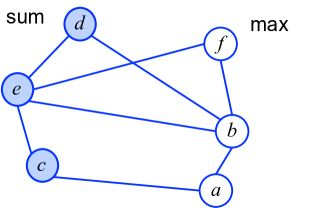
  Refer to caption Refer to caption
(a) (b)
Figure 3: (a) An example of marginal MAP problem, where d,c,e𝑑𝑐𝑒d,c,e are sum nodes (shaded) and a,b,f𝑎𝑏𝑓a,b,f are max nodes. (b) A junction graph of (a). Selecting a partitioning of max nodes, πbde=πbef=subscript𝜋𝑏𝑑𝑒subscript𝜋𝑏𝑒𝑓\pi_{bde}=\pi_{bef}=\emptyset, πabc={a,b}subscript𝜋𝑎𝑏𝑐𝑎𝑏\pi_{abc}=\{a,b\}, and πbef={f}subscript𝜋𝑏𝑒𝑓𝑓\pi_{bef}=\{f\}, results in {bde},{bce}𝑏𝑑𝑒𝑏𝑐𝑒\{bde\},\{bce\} being sum clusters (shaded) and {abc},{bef}𝑎𝑏𝑐𝑏𝑒𝑓\{abc\},\{bef\} being max clusters.

Overall, the marginal MAP dual form in (12) is approximated by

max𝝉𝕃(𝒢){𝜽,𝝉+k𝒜Hck(𝝉)+kHck|πk(𝝉)(kl)Hskl(𝝉)}subscript𝝉𝕃𝒢𝜽𝝉subscript𝑘𝒜subscript𝐻subscript𝑐𝑘𝝉subscript𝑘subscript𝐻conditionalsubscript𝑐𝑘subscript𝜋𝑘𝝉subscript𝑘𝑙subscript𝐻subscript𝑠𝑘𝑙𝝉\displaystyle\max_{{\boldsymbol{\tau}}\in\mathbb{L}(\mathcal{G})}\big{\{}\langle\boldsymbol{\theta},{\boldsymbol{\tau}}\rangle+\sum_{k\in\mathcal{A}}H_{c_{k}}({\boldsymbol{\tau}})+\sum_{k\in\mathcal{B}}H_{c_{k}|\pi_{k}}({\boldsymbol{\tau}})-\sum_{(kl)\in\mathcal{E}}H_{s_{kl}}({\boldsymbol{\tau}})\big{\}} (51)

where Hck|πk(𝝉)=Hck(𝝉)Hπk(𝝉)subscript𝐻conditionalsubscript𝑐𝑘subscript𝜋𝑘𝝉subscript𝐻subscript𝑐𝑘𝝉subscript𝐻subscript𝜋𝑘𝝉H_{c_{k}|\pi_{k}}({\boldsymbol{\tau}})=H_{c_{k}}({\boldsymbol{\tau}})-H_{\pi_{k}}({\boldsymbol{\tau}}). Optimizing (51) using a method similar to the derivation of mixed-product BP in Algorithm 2, we obtain a “mixed-product” junction graph belief propagation, given in Algorithm 5.

Algorithm 5 Mixed-product Junction Graph BP
  1. Passing messages between clusters on the junction graph until convergence:
𝒜𝒜𝒜𝒜\mathcal{A}\to\mathcal{A}\cup\mathcal{B}:
(sum-product)
mkl(xskl)xcksklψck(xck)mkl(xck),proportional-tosubscript𝑚𝑘𝑙subscript𝑥subscript𝑠𝑘𝑙subscriptsubscript𝑥subscript𝑐𝑘subscript𝑠𝑘𝑙subscript𝜓subscript𝑐𝑘subscript𝑥subscript𝑐𝑘subscript𝑚similar-toabsent𝑘𝑙subscript𝑥subscript𝑐𝑘\displaystyle m_{k\to l}(x_{s_{kl}})\propto\sum_{x_{c_{k}\setminus s_{kl}}}\psi_{c_{k}}(x_{c_{k}})m_{\sim k\setminus l}(x_{c_{k}}),
𝒜𝒜\mathcal{B}\to\mathcal{A}\cup\mathcal{B}:
(argmax-product)
mkl(xskl)xckskl(ψck(xck)mkl(xck))𝟏[xπk𝒳πk],proportional-tosubscript𝑚𝑘𝑙subscript𝑥subscript𝑠𝑘𝑙subscriptsubscript𝑥subscript𝑐𝑘subscript𝑠𝑘𝑙subscript𝜓subscript𝑐𝑘subscript𝑥subscript𝑐𝑘subscript𝑚similar-toabsent𝑘𝑙subscript𝑥subscript𝑐𝑘1delimited-[]subscript𝑥subscript𝜋𝑘subscriptsuperscript𝒳subscript𝜋𝑘\displaystyle m_{k\to l}(x_{s_{kl}})\propto\sum_{x_{c_{k}\setminus s_{kl}}}(\psi_{c_{k}}(x_{c_{k}})m_{\sim k\setminus l}(x_{c_{k}}))\cdot\boldsymbol{1}[x_{\pi_{k}}\in\mathcal{X}^{*}_{\pi_{k}}],
where 𝒳πk=argmaxxπkxckπkbk(xck)subscriptsuperscript𝒳subscript𝜋𝑘subscriptargmaxsubscript𝑥subscript𝜋𝑘subscriptsubscript𝑥subscript𝑐𝑘subscript𝜋𝑘subscript𝑏𝑘subscript𝑥subscript𝑐𝑘\mathcal{X}^{*}_{\pi_{k}}=\operatorname*{arg\,max}_{x_{\pi_{k}}}\sum_{x_{c_{k}\setminus\pi_{k}}}b_{k}(x_{c_{k}}),
         bk(xck)=ψck(xck)k𝒩(k)mkk(xskk)subscript𝑏𝑘subscript𝑥subscript𝑐𝑘subscript𝜓subscript𝑐𝑘subscript𝑥subscript𝑐𝑘subscriptproductsuperscript𝑘𝒩𝑘subscript𝑚superscript𝑘𝑘subscript𝑥subscript𝑠superscript𝑘𝑘b_{k}(x_{c_{k}})=\psi_{c_{k}}(x_{c_{k}})\!\!\!\prod_{k^{\prime}\in\mathcal{N}(k)}\!\!\!m_{k^{\prime}\to k}(x_{s_{k^{\prime}k}})   and   mkl(xck)=k𝒩(k){l}mkk(xskk)subscript𝑚similar-toabsent𝑘𝑙subscript𝑥subscript𝑐𝑘subscriptproductsuperscript𝑘𝒩𝑘𝑙subscript𝑚superscript𝑘𝑘subscript𝑥subscript𝑠superscript𝑘𝑘m_{\sim k\setminus l}(x_{c_{k}})~{}=\!\!\!\!\!\!\!\prod_{k^{\prime}\in\mathcal{N}(k)\setminus\{l\}}\!\!\!\!\!\!m_{k^{\prime}\to k}(x_{s_{k^{\prime}k}}).
  2. Decoding: 𝒙πk=argmaxxπkxckπkbk(xck)subscriptsuperscript𝒙subscript𝜋𝑘subscriptargmaxsubscript𝑥subscript𝜋𝑘subscriptsubscript𝑥subscript𝑐𝑘subscript𝜋𝑘subscript𝑏𝑘subscript𝑥subscript𝑐𝑘\displaystyle\boldsymbol{x}^{*}_{\pi_{k}}=\operatorname*{arg\,max}_{x_{\pi_{k}}}\sum_{x_{c_{k}\setminus\pi_{k}}}b_{k}(x_{c_{k}}) for kfor-all𝑘\forall k\in\mathcal{B}.

Similarly to our mixed-product BP in Algorithm 2, Algorithm 5 also admits an intuitive reparameterization interpretation and a strong local optimality guarantee. Algorithm 5 can be seen as a special case of a more general junction graph BP algorithm derived in Liu and Ihler (2012) for solving maximum expected utility tasks in decision networks. For more details, we refer the reader to that work.

9 Experiments

We illustrate our algorithms on both simulated models and more realistic diagnostic Bayesian networks taken from the UAI08 inference challenge. We show that our Bethe approximation algorithms perform best among all the tested algorithms, including Jiang et al. (2011)’s hybrid message passing and a state-of-the-art local search algorithm (Park and Darwiche, 2004).

We implement our mixed-product BP in Algorithm 2 with Bethe weights (mix-product (Bethe)), the regular sum-product BP (sum-product), max-product BP (max-product) and Jiang et al. (2011)’s hybrid message passing (with Bethe weights) in Algorithm 3 (Jiang’s method), where the solutions are all extracted by maximizing the singleton marginals of the max nodes. For all these algorithms, we run a maximum of 50 iterations; in case they fail to converge, we run 100 additional iterations with a damping coefficient of 0.10.10.1. We initialize all these algorithms with 5 random initializations and pick the best solution; for mix-product (Bethe) and Jiang’s method, we run an additional trial initialized using the sum-product messages, which was reported to perform well in Park and Darwiche (2004) and Jiang et al. (2011). We also run the proximal point version of mixed-product BP with Bethe weights (Proximal (Bethe) ), which is Algorithm 4 with both HA|B(𝝉)subscript𝐻conditional𝐴𝐵𝝉H_{A|B}({\boldsymbol{\tau}}) and HB(𝝉)subscript𝐻𝐵𝝉H_{B}({\boldsymbol{\tau}}) approximated by Bethe approximations.

We also implement the TRW approximation, but only using the convergent proximal point algorithm, because the TRW upper bounds are valid only when the algorithms converge. The TRW weights of H^A|Bsubscript^𝐻conditional𝐴𝐵\hat{H}_{A|B} are constructed by first (randomly) selecting spanning trees of GAsubscript𝐺𝐴G_{A}, and then augmenting each spanning tree with one uniformly selected edge in ABsubscript𝐴𝐵\partial_{AB}; the TRW weights of H^B(𝝉)subscript^𝐻𝐵𝝉\hat{H}_{B}({\boldsymbol{\tau}}) are constructed to be provably convex, using the method of TRW-S in Kolmogorov (2006). We run all the proximal point algorithms for a maximum of 100 iterations, with a maximum of 5 iterations of weighted message passing updates (28)-(29) for the inner loops (with 5 additional damping with 0.1 damping coefficient).

In addition, we compare our algorithms with SamIam, which is a state-of-the-art implementation of the local search algorithm for marginal MAP (Park and Darwiche, 2004); we use its default Taboo search method with a maximum of 500 searching steps, and report the best results among 5 trials with random initializations, and one additional trial initialized by its default method (which sequentially initializes xisubscript𝑥𝑖x_{i} by maximizing p(xi|xpai)𝑝conditionalsubscript𝑥𝑖subscript𝑥subscriptpa𝑖p(x_{i}|x_{\mathrm{pa}_{i}}) along some predefined order).

We also implement an EM algorithm, whose expectation and maximization steps are approximated by sum-product and max-product BP, respectively. We run EM with 5 random initializations and one initialization by sum-product marginals, and pick the best solution.

Simulated Models. We consider pairwise models over discrete random variables taking values in {1,0,+1}nsuperscript101𝑛\{-1,0,+1\}^{n},

p(𝒙)exp[iθi(xi)+(ij)Eθij(xi,xj)].proportional-to𝑝𝒙subscript𝑖subscript𝜃𝑖subscript𝑥𝑖subscript𝑖𝑗𝐸subscript𝜃𝑖𝑗subscript𝑥𝑖subscript𝑥𝑗p(\boldsymbol{x})\propto\exp\big{[}\sum_{i}\theta_{i}(x_{i})+\sum_{(ij)\in E}\theta_{ij}(x_{i},x_{j})\big{]}.

The value tables of θisubscript𝜃𝑖\theta_{i} and θijsubscript𝜃𝑖𝑗\theta_{ij} are randomly generated from normal distribution, θi(k)Normal(0,0.01)similar-tosubscript𝜃𝑖𝑘Normal00.01\theta_{i}(k)\sim\mathrm{Normal}(0,0.01), θij(k,l)Normal(0,σ2)similar-tosubscript𝜃𝑖𝑗𝑘𝑙Normal0superscript𝜎2\theta_{ij}(k,l)\sim\mathrm{Normal}(0,\sigma^{2}), where σ𝜎\sigma controls the strength of coupling. Our results are averaged on 1000 randomly generated sets of parameters.

We consider different choices of graph structures and max / sum node patterns:

  1. 1.

    Hidden Markov chain with 20 nodes, as shown in Fig. 1.

  2. 2.

    Latent tree models. We generate random trees of size 50, by finding the minimum spanning trees of random symmetric matrices with elements drawn from Uniform([0,1])Uniform01\mathrm{Uniform}([0,1]). We take the leaf nodes to be max nodes, and the non-leaf nodes to be sum nodes. See Fig. 5(a) for a typical example.

  3. 3.

    10×10101010\times 10 Grid with max and sum nodes distributed in two opposite chess board patterns shown in Fig. 6(a) and Fig. 7(a), respectively. In Fig. 6(a), the sum part is a loopy graph, and the max part is a (fully disconnected) tree; in Fig. 7(a), the max and sum parts are flipped.

The results on the hidden Markov chain are shown in Fig. 4, where we plot in panel (a) different algorithms’ percentages of obtaining the globally optimal solutions among 1000 random trials, and in panel (b) their relative energy errors defined by Q(𝒙^B;𝜽)Q(𝒙B;𝜽)𝑄subscript^𝒙𝐵𝜽𝑄superscriptsubscript𝒙𝐵𝜽Q(\hat{\boldsymbol{x}}_{B};\boldsymbol{\theta})-Q(\boldsymbol{x}_{B}^{*};\boldsymbol{\theta}), where 𝒙^Bsubscript^𝒙𝐵\hat{\boldsymbol{x}}_{B} is the solution returned by the algorithms, and 𝒙Bsuperscriptsubscript𝒙𝐵\boldsymbol{x}_{B}^{*} is the true optimum.

The results of the latent tree models and the two types of 2D grids are shown in Fig. 5, Fig. 6 and Fig. 7, respectively. Since the globally optimal solution 𝒙Bsuperscriptsubscript𝒙𝐵\boldsymbol{x}_{B}^{*} is not tractable to calculate in these cases, we report the approximate relative error defined by Q(𝒙^B;𝜽)Q(𝒙~B;𝜽)𝑄subscript^𝒙𝐵𝜽𝑄subscript~𝒙𝐵𝜽Q(\hat{\boldsymbol{x}}_{B};\boldsymbol{\theta})-Q(\tilde{\boldsymbol{x}}_{B};\boldsymbol{\theta}), where 𝒙~Bsubscript~𝒙𝐵\tilde{\boldsymbol{x}}_{B} is the best solution we found across all algorithms.

Diagnostic Bayesian Networks. We also test our algorithms on two diagnostic Bayesian networks taken from the UAI08 Inference Challenge, where we construct marginal MAP problems by randomly selecting varying percentages of nodes to be max nodes. Since these models are not pairwise, we implement the junction graph versions of mix-product (Bethe) and proximal (Bethe) shown in Section 8. Fig. 8 shows the approximate relative errors of our algorithms and local search (SamIam) as the percentage of the max nodes varies.

Insights. Across all the experiments, we find that mix-product (Bethe), proximal (Bethe) and local search (SamIam) significantly outperform all the other algorithms, while proximal (Bethe) outperforms the two others in some circumstances. In the hidden Markov chain example in Fig. 4, these three algorithms almost always (with probability 99%absentpercent99\geq 99\%) find the globally optimal solutions. However, the performance of SamIam tends to degenerate when the max part has loopy dependency structures (see Fig. 7), or when the number of max nodes is large (see Fig. 8), both of which make it difficult to explore the solution space by local search. On the other hand, mix-product (Bethe) tends to degenerate as the coupling strength σ𝜎\sigma increases (see Fig. 7), probably because its convergence gets worse as σ𝜎\sigma increases.

We note that our TRW approximation gives much less accurate solutions than the other algorithms, but is able to provide an upper bound on the optimal energy. Similar phenomena have been observed for TRW-BP in standard max- and sum- inference.

The hybrid message passing of Jiang et al. (2011) is significantly worse than mix-product (Bethe), proximal (Bethe) and local search (SamIam), but is otherwise the best among the remaining algorithms. EM performs similarly to (or sometimes worse than) Jiang’s method.

The regular max-product BP and sum-product BP are among the worst of the tested algorithms, indicating the danger of approximating mixed-inference by pure max- or sum- inference. Interestingly, the performances of max-product BP and sum-product BP have opposite trends: In Fig. 4, Fig. 5 and Fig. 6, where the max parts are fully disconnected and the sum parts are connected and loopy, max-product BP usually performs worse than sum-product BP, but gets better as the coupling strength σ𝜎\sigma increases; sum-product BP, on the other hand, tends to degenerate as σ𝜎\sigma increases. In Fig. 7, where the max / sum pattern is reversed (resulting in a larger, loopier max subgraph), max-product BP performs better than sum-product BP.
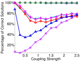
​​​​​​
Refer to caption
         
Refer to caption

Refer to caption

(a) (b) Refer to caption
Figure 4: Results on the hidden Markov chain in Fig. 1 (best viewed in color). (a) different algorithms’ probabilities of obtaining the globally optimal solution among 1000 random trials. Mix-product (Bethe), Proximal (Bethe) and Local Search (SamIam) almost always (with probability 99%absentpercent99\geq 99\%) find the optimal solution. (b) The relative energy errors of the different algorithms, and the upper bounds obtained by Proximal (TRW) as a function of coupling strength σ𝜎\sigma.
​​​​​​ Refer to caption             
Refer to caption

Refer to caption

(a) (b) Refer to caption
Figure 5: (a) A typical latent tree model, whose leaf nodes are taken to be max nodes (white) and non-leaf nodes to be sum nodes (shaded). (b) The approximate relative energy errors of different algorithms, and the upper bound obtained by Proximal (TRW) as a function of coupling strength σ𝜎\sigma.
Refer to caption Refer to caption
Refer to caption

Refer to caption

(a) (b)
Figure 6: (a) A marginal MAP problem defined on a 10×10101010\times 10 Ising grid, with shaded sum nodes and unshaded max nodes; note that the sum part is a loopy graph, while max part is fully disconnected. (b) The approximate relative errors of different algorithms and the upper bound obtained by Proximal (TRW) as a function of coupling strength σ𝜎\sigma.
Refer to caption Refer to caption
Refer to caption

Refer to caption

(a) (b)
Figure 7: (a) A marginal MAP problem defined on a 10×10101010\times 10 Ising grid, but with max / sum part exactly opposite to that in Fig. 6; note that the max part is loopy, while the sum part is fully disconnected in this case. (b) The approximate relative errors of different algorithms and the upper bound obtained by Proximal (TRW) as a function of coupling strength σ𝜎\sigma.
Refer to caption
(a) The structure of Diagnostic BN-2, with 50% randomly selected sum nodes shaded.
Refer to caption Refer to caption
(b) Diagnostic BN-1 (c) Diagnostic BN-2
Refer to caption
Figure 8: The results on two diagnostic Bayesian networks (BNs) in the UAI08 inference challenge. (a) The Diagnostic BN-2 network. (b)-(c) The performances of algorithms on the two BNs as a function of the percentage of max nodes. The local search method tends to degenerate when the number of max nodes is large, making it difficult to search over the solution space. Results are averaged over 100 random trials.

10 Conclusion and Further Directions

We have presented a general variational framework for solving marginal MAP problems approximately, opening new doors for developing efficient algorithms. In particular, we show that our proposed “mixed-product” BP admits appealing theoretical properties and performs well in practice.

Potential future directions include improving the performance of the truncated TRW approximation by optimizing weights, deriving optimality conditions that may be applicable even when the sum component does not form a tree, studying the convergent properties of mixed-product BP, and leveraging our results to learn hidden variable models for data.

Acknowledgments

We thank Arthur Choi for providing help on SamIam. This work was supported in part by the National Science Foundation (awards IIS-1065618 and IIS-1254071), and a Microsoft Research Ph.D Fellowship.

References

  • Altarelli et al. (2011) F. Altarelli, A. Braunstein, A. Ramezanpour, and R. Zecchina. Stochastic optimization by message passing. Journal of Statistical Mechanics: Theory and Experiment, 2011(11):P11009, 2011.
  • Birge and Louveaux (1997) J.R. Birge and F. Louveaux. Introduction to stochastic programming. Springer Verlag, 1997.
  • Boyd et al. (2010) S. Boyd, N. Parikh, E. Chu, B. Peleato, and J. Eckstein. Distributed optimization and statistical learning via the alternating direction method of multipliers. Foundations and Trends in Machine Learning, 2010.
  • Cover and Thomas (2006) T.M. Cover and J.A. Thomas. Elements of Information Theory. John Wiley & Sons, INC., 2nd edition, 2006.
  • De Campos (2011) C.P. De Campos. New complexity results for MAP in Bayesian networks. In Proceedings of the 22nd International Joint Conference on Artificial Intelligence (IJCAI-11), pages 2100–2106, 2011.
  • Dechter and Rish (2003) R. Dechter and I. Rish. Mini-buckets: A general scheme for bounded inference. Journal of the ACM (JACM), 50(2):107–153, 2003.
  • Doucet et al. (2002) A. Doucet, S.J. Godsill, and C.P. Robert. Marginal maximum a posteriori estimation using Markov chain Monte Carlo. Statistics and Computing, 12(1), January 2002.
  • Globerson and Jaakkola (2007) A. Globerson and T.S. Jaakkola. Approximate inference using conditional entropy decompositions. In Proceedings of the Eleventh International Conference on Artificial Intelligence and Statistics (AISTATS-07), 2007.
  • Greig et al. (1989) D.M. Greig, B.T. Porteous, and A.H. Seheult. Exact maximum a posteriori estimation for binary images. Journal of the Royal Statistical Society. Series B (Methodological), pages 271–279, 1989.
  • Hazan and Shashua (2010) T. Hazan and A. Shashua. Norm-product belief propagation: Primal-dual message-passing for approximate inference. Information Theory, IEEE Transactions on, 56(12):6294–6316, 2010.
  • Hazan et al. (2012) T. Hazan, J. Peng, and A. Shashua. Tightening fractional covering upper bounds on the partition function for high-order region graphs. In Proceedings of the 28th conference on Uncertainty in artificial intelligence (UAI-12), 2012.
  • Howard and Matheson (2005) R.A. Howard and J.E. Matheson. Influence diagrams. Decision Analysis, 2(3):127–143, 2005.
  • Hunter and Lange (2004) D.R. Hunter and K. Lange. A tutorial on MM algorithms. The American Statistician, 1(58), February 2004.
  • Ibrahimi et al. (2011) M. Ibrahimi, A. Javanmard, Y. Kanoria, and A. Montanari. Robust max-product belief propagation. In Signals, Systems and Computers (ASILOMAR), 2011 Conference Record of the Forty Fifth Asilomar Conference on, pages 43–49. IEEE, 2011.
  • Iusem and Teboulle (1993) A. Iusem and M. Teboulle. On the convergence rate of entropic proximal optimization methods. Computational and Applied Mathematics, 12:153–168, 1993.
  • Jaynes (1957) E.T. Jaynes. Information theory and statistical mechanics. Physical Review, 106(4):620–630, May 1957.
  • Jerrum and Sinclair (1993) M. Jerrum and A. Sinclair. Polynomial-time approximation algorithms for the ising model. SIAM Journal on computing, 22(5):1087–1116, 1993.
  • Jiang et al. (2011) J. Jiang, P. Rai, and H. Daumé III. Message-passing for approximate map inference with latent variables. In Advances in Neural Information Processing Systems (NIPS-11), 2011.
  • Jojic et al. (2010) V. Jojic, S. Gould, and D. Koller. Accelerated dual decomposition for MAP inference. In Proceedings of the 27th International Conference on Machine Learning (ICML-10), 2010.
  • Koller and Friedman (2009) D. Koller and N. Friedman. Probabilistic graphical models: principles and techniques. MIT press, 2009.
  • Kolmogorov (2006) V. Kolmogorov. Convergent tree-reweighted message passing for energy minimization. Pattern Analysis and Machine Intelligence, IEEE Transactions on, 28(10):1568 –1583, oct. 2006.
  • Liu and Ihler (2011a) Q. Liu and A. Ihler. Bounding the partition function using Hölder’s inequality. In Proceedings of the 28th International Conference on Machine Learning (ICML-11), pages 849–856, June 2011a.
  • Liu and Ihler (2011b) Q. Liu and A. Ihler. Variational algorithms for marginal MAP. In Proceedings of the 27th Conference on Uncertainty in Artificial Intelligence (UAI-11). 2011b.
  • Liu and Ihler (2012) Q. Liu and A. Ihler. Belief propagation for structured decision making. In Proceedings of the 28th Conference on Uncertainty in Artificial Intelligence (UAI-12). August 2012.
  • Martinet (1970) B. Martinet. Régularisation d’inéquations variationnelles par approximations successives. Revue Française d Informatique et de Recherche Opérationelle, 4:154–158, 1970.
  • Mateescu et al. (2010) R. Mateescu, K. Kask, V. Gogate, and R. Dechter. Join-graph propagation algorithms. Journal of Artificial Intelligence Research, 37(1):279–328, 2010.
  • Mauá and de Campos (2012) D.D. Mauá and C.P. de Campos. Anytime marginal maximum a posteriori inference. In Proceedings of the 29th International Conference on Machine Learning (ICML-12), 2012.
  • Meltzer et al. (2009) T. Meltzer, A. Globerson, and Y. Weiss. Convergent message passing algorithms: a unifying view. In Proceedings of the 25th Conference on Uncertainty in Artificial Intelligence (UAI-09), 2009.
  • Meshi et al. (2012) O.P. Meshi, T. Jaakkola, and A. Globerson. Convergence rate analysis of MAP coordinate minimization algorithms. In Advances in Neural Information Processing Systems (NIPS-12), 2012.
  • Neal and Hinton (1998) R. Neal and G.E. Hinton. A view of the EM algorithm that justifies incremental, sparse, and other variants. In M. Jordan, editor, Learning in Graphical Models, pages 355–368. Kluwer, 1998.
  • Park and Darwiche (2004) J. Park and A. Darwiche. Complexity results and approximation strategies for MAP explanations. Journal of Artificial Intelligence Research, 21:101–133, 2004.
  • Pearl (1988) J. Pearl. Probabilistic reasoning in intelligent systems: networks of plausible inference. Morgan Kaufmann, 1988.
  • Ravikumar et al. (2010) P. Ravikumar, A. Agarwal, and M.J. Wainwright. Message-passing for graph-structured linear programs: Proximal projections, convergence, and rounding schemes. Journal of Machine Learning Research, 11:1043–1080, Mar 2010.
  • Rockafellar (1976) R.T. Rockafellar. Monotone operators and the proximal point algorithm. SIAM Journal on Control and Optimization, 14(5):877, 1976.
  • Savchynskyy et al. (2010) B. Savchynskyy, S. Schmidt, J.H. Kappes, and C. Schnörr. Efficient MRF energy minimization via adaptive diminishing smoothing. In Proceedings of the 28th Conference on Uncertainty in Artificial Intelligence (UAI-12), 2010.
  • Sontag et al. (2011) D. Sontag, A. Globerson, and T.S. Jaakkola. Introduction to dual decomposition for inference. In Optimization for Machine Learning. MIT Press, 2011.
  • Teboulle (1992) M. Teboulle. Entropic proximal mappings with applications to nonlinear programming. Mathematics of Operations Research, 17(3):pp. 670–690, 1992.
  • Tseng and Bertsekas (1993) P. Tseng and D.P. Bertsekas. On the convergence of the exponential multiplier method for convex programming. Mathematical Programming, 60(1):1–19, 1993.
  • Wainwright and Jordan (2008) M.J. Wainwright and M. Jordan. Graphical models, exponential families, and variational inference. Foundation and Trends in Machine Learning, 1(1-2):1–305, 2008.
  • Wainwright et al. (2003) M.J. Wainwright, T.S. Jaakkola, and A.S. Willsky. Tree-based reparameterization framework for analysis of sum-product and related algorithms. Information Theory, IEEE Transactions on, 45:1120–1146, 2003.
  • Wainwright et al. (2005a) M.J. Wainwright, T.S. Jaakkola, and A.S. Willsky. A new class of upper bounds on the log partition function. Information Theory, IEEE Transactions on, 51(7):2313–2335, July 2005a.
  • Wainwright et al. (2005b) M.J. Wainwright, T.S. Jaakkola, and A.S. Willsky. MAP estimation via agreement on trees: message-passing and linear programming. Information Theory, IEEE Transactions on, 51(11):3697–3717, 2005b.
  • Weiss et al. (2007) Y. Weiss, C. Yanover, and T. Meltzer. MAP estimation, linear programming and belief propagation with convex free energies. In Proceedings of the 23rd conference on Uncertainty in Artificial Intelligence (UAI-07), 2007.
  • Werner (2007) T. Werner. A linear programming approach to max-sum problem: A review. Pattern Analysis and Machine Intelligence, IEEE Transactions on, 29(7):1165–1179, 2007.
  • Werner (2010) T. Werner. Revisiting the linear programming relaxation approach to Gibbs energy minimization and weighted constraint satisfaction. Pattern Analysis and Machine Intelligence, IEEE Transactions on, 32(8):1474–1488, 2010.
  • Wiegerinck (2005) W. Wiegerinck. Approximations with reweighted generalized belief propagation. In In Proceedings of the 9th International Conference on Artificial Intelligence and Statistics (AISTATS-05), 2005.
  • Yedidia et al. (2003) J.S. Yedidia, W.T. Freeman, and Y. Weiss. Understanding belief propagation and its generalizations. Exploring artificial intelligence in the new millennium, 8:236–239, 2003.
  • Yedidia et al. (2005) J.S. Yedidia, W.T. Freeman, and Y. Weiss. Constructing free-energy approximations and generalized BP algorithms. Information Theory, IEEE Transactions on, 51, July 2005.
  • Yuan et al. (2004) C. Yuan, T.C. Lu, and M.J. Druzdzel. Annealed MAP. In Proceedings of the 20th conference on Uncertainty in artificial intelligence (UAI-04), pages 628–635, 2004.
  • Yuille (2002) A. L. Yuille. CCCP algorithms to minimize the Bethe and Kikuchi free energies: Convergent alternatives to belief propagation. Neural Computation, 14(7):1691–1722, July 2002.

A Proof of Proposition 6

Proof.

The Lagrangian of (21) with the local consistency constraint of 𝕃𝕃\mathbb{L} in (5) is

𝜽,𝝉+iV[wiHi(𝝉)+λi0xiτi(xi)](ij)E[wijIij(𝝉)+xjλij(xj)xi(τij(xi,xj)τj(xj))].𝜽𝝉subscript𝑖𝑉delimited-[]subscript𝑤𝑖subscript𝐻𝑖𝝉superscriptsubscript𝜆𝑖0subscriptsubscript𝑥𝑖subscript𝜏𝑖subscript𝑥𝑖subscript𝑖𝑗𝐸delimited-[]subscript𝑤𝑖𝑗subscript𝐼𝑖𝑗𝝉subscriptsubscript𝑥𝑗subscript𝜆𝑖𝑗subscript𝑥𝑗subscriptsubscript𝑥𝑖subscript𝜏𝑖𝑗subscript𝑥𝑖subscript𝑥𝑗subscript𝜏𝑗subscript𝑥𝑗\langle\boldsymbol{\theta},{\boldsymbol{\tau}}\rangle+\sum_{i\in V}[w_{i}H_{i}({\boldsymbol{\tau}})+\lambda_{i}^{0}\sum_{x_{i}}\tau_{i}(x_{i})]-\sum_{(ij)\in E}[w_{ij}I_{ij}({\boldsymbol{\tau}})+\sum_{x_{j}}\lambda_{i\to j}(x_{j})\sum_{x_{i}}(\tau_{ij}(x_{i},x_{j})-\tau_{j}(x_{j}))].

where {λi0:iV}conditional-setsuperscriptsubscript𝜆𝑖0𝑖𝑉\{\lambda_{i}^{0}\colon i\in V\} and {λji(xi):(ij)E,xi𝒳i}conditional-setsubscript𝜆𝑗𝑖subscript𝑥𝑖formulae-sequence𝑖𝑗𝐸subscript𝑥𝑖subscript𝒳𝑖\{\lambda_{j\to i}(x_{i})\colon(ij)\in E,x_{i}\in\mathcal{X}_{i}\} are the Lagrange multipliers. Recall that

𝜽,𝝉=iVθi(xi)τi(xi)+(ij)Eθij(xi,xj)τij(xi,xj),𝜽𝝉subscript𝑖𝑉subscript𝜃𝑖subscript𝑥𝑖subscript𝜏𝑖subscript𝑥𝑖subscript𝑖𝑗𝐸subscript𝜃𝑖𝑗subscript𝑥𝑖subscript𝑥𝑗subscript𝜏𝑖𝑗subscript𝑥𝑖subscript𝑥𝑗\displaystyle\langle\boldsymbol{\theta},{\boldsymbol{\tau}}\rangle=\sum_{i\in V}\theta_{i}(x_{i})\tau_{i}(x_{i})+\sum_{(ij)\in E}\theta_{ij}(x_{i},x_{j})\tau_{ij}(x_{i},x_{j}),
Hi(𝝉)=xiτi(xi)logτi(xi),subscript𝐻𝑖𝝉subscriptsubscript𝑥𝑖subscript𝜏𝑖subscript𝑥𝑖subscript𝜏𝑖subscript𝑥𝑖\displaystyle H_{i}({\boldsymbol{\tau}})=-\sum_{x_{i}}\tau_{i}(x_{i})\log\tau_{i}(x_{i}),
Iij(𝝉)=xi,xjτij(xi,xj)logτij(xi,xj)xiτij(xi,xj)xjτij(xi,xj).subscript𝐼𝑖𝑗𝝉subscriptsubscript𝑥𝑖subscript𝑥𝑗subscript𝜏𝑖𝑗subscript𝑥𝑖subscript𝑥𝑗subscript𝜏𝑖𝑗subscript𝑥𝑖subscript𝑥𝑗subscriptsubscript𝑥𝑖subscript𝜏𝑖𝑗subscript𝑥𝑖subscript𝑥𝑗subscriptsubscript𝑥𝑗subscript𝜏𝑖𝑗subscript𝑥𝑖subscript𝑥𝑗\displaystyle I_{ij}({\boldsymbol{\tau}})=\sum_{x_{i},x_{j}}\tau_{ij}(x_{i},x_{j})\log\frac{\tau_{ij}(x_{i},x_{j})}{\sum_{x_{i}}\tau_{ij}(x_{i},x_{j})\sum_{x_{j}}\tau_{ij}(x_{i},x_{j})}.

Taking the derivative of the Lagrangian w.r.t. τi(xi)subscript𝜏𝑖subscript𝑥𝑖\tau_{i}(x_{i}) and τij(xi,xj)subscript𝜏𝑖𝑗subscript𝑥𝑖subscript𝑥𝑗\tau_{ij}(x_{i},x_{j}), we have

θi(xi)wilogτi(xi)+jiλji(xi)=const,subscript𝜃𝑖subscript𝑥𝑖subscript𝑤𝑖subscript𝜏𝑖subscript𝑥𝑖subscript𝑗subscript𝑖subscript𝜆𝑗𝑖subscript𝑥𝑖𝑐𝑜𝑛𝑠𝑡\displaystyle\theta_{i}(x_{i})-w_{i}\log\tau_{i}(x_{i})+\sum_{j\in\partial_{i}}\lambda_{j\to i}(x_{i})=const, (52)
θij(xi,xj)wijlogτij(xi,xj)τi(xi)τj(xj)+λij(xj)+λji(xi)=const,subscript𝜃𝑖𝑗subscript𝑥𝑖subscript𝑥𝑗subscript𝑤𝑖𝑗subscript𝜏𝑖𝑗subscript𝑥𝑖subscript𝑥𝑗subscript𝜏𝑖subscript𝑥𝑖subscript𝜏𝑗subscript𝑥𝑗subscript𝜆𝑖𝑗subscript𝑥𝑗subscript𝜆𝑗𝑖subscript𝑥𝑖𝑐𝑜𝑛𝑠𝑡\displaystyle\theta_{ij}(x_{i},x_{j})-w_{ij}\log\frac{\tau_{ij}(x_{i},x_{j})}{\tau_{i}(x_{i})\tau_{j}(x_{j})}+\lambda_{i\to j}(x_{j})+\lambda_{j\to i}(x_{i})=const, (53)

where we used the local consistency condition that xjτij(xi,xj)=τi(xi)subscriptsubscript𝑥𝑗subscript𝜏𝑖𝑗subscript𝑥𝑖subscript𝑥𝑗subscript𝜏𝑖subscript𝑥𝑖\sum_{x_{j}}\tau_{ij}(x_{i},x_{j})=\tau_{i}(x_{i}). By defining mij(xj)=exp(λij(xj))subscript𝑚𝑖𝑗subscript𝑥𝑗subscript𝜆𝑖𝑗subscript𝑥𝑗m_{i\to j}(x_{j})=\exp(\lambda_{i\to j}(x_{j})), we obtain (29) directly from (52)-(53).
Plugging (29) into the constraint that xjτij(xi,xj)=τi(xi)subscriptsubscript𝑥𝑗subscript𝜏𝑖𝑗subscript𝑥𝑖subscript𝑥𝑗subscript𝜏𝑖subscript𝑥𝑖\sum_{x_{j}}\tau_{ij}(x_{i},x_{j})=\tau_{i}(x_{i}) gives (28). ∎

B Proof of Theorem 5

Proof.

(i). For 𝝉𝕄o𝝉superscript𝕄𝑜{\boldsymbol{\tau}}\in\mathbb{M}^{o}, the objective function in (19) equals

Ftree(𝝉,𝜽)subscript𝐹𝑡𝑟𝑒𝑒𝝉𝜽\displaystyle F_{tree}({\boldsymbol{\tau}},\boldsymbol{\theta}) =𝜽,𝝉+iVHi(𝝉)(ij)EAIij(𝝉)(ij)ABρijIij(𝝉)absent𝜽𝝉subscript𝑖𝑉subscript𝐻𝑖𝝉subscript𝑖𝑗subscript𝐸𝐴subscript𝐼𝑖𝑗𝝉subscript𝑖𝑗subscript𝐴𝐵subscript𝜌𝑖𝑗subscript𝐼𝑖𝑗𝝉\displaystyle=\langle\boldsymbol{\theta},{\boldsymbol{\tau}}\rangle\ +\ \sum_{i\in V}H_{{i}}({\boldsymbol{\tau}})-\!\!\!\sum_{(ij)\in E_{A}}\!\!\!I_{{ij}}({\boldsymbol{\tau}})-\!\!\!\sum_{(ij)\in\partial_{AB}}\!\!\!\!\rho_{ij}I_{{ij}}({\boldsymbol{\tau}})
=𝜽,𝝉+iVHi(𝝉)(ij)EAIij(𝝉)absent𝜽𝝉subscript𝑖𝑉subscript𝐻𝑖𝝉subscript𝑖𝑗subscript𝐸𝐴subscript𝐼𝑖𝑗𝝉\displaystyle=\langle\boldsymbol{\theta},{\boldsymbol{\tau}}\rangle\ +\ \sum_{i\in V}H_{{i}}({\boldsymbol{\tau}})-\!\!\!\sum_{(ij)\in E_{A}}\!\!\!I_{{ij}}({\boldsymbol{\tau}}) (54)
=𝜽,𝝉+HA|B(𝝉)absent𝜽𝝉subscript𝐻conditional𝐴𝐵𝝉\displaystyle=\langle\boldsymbol{\theta},{\boldsymbol{\tau}}\rangle\ +H_{A|B}({\boldsymbol{\tau}}) (55)
=Fmix(𝝉,𝜽),absentsubscript𝐹𝑚𝑖𝑥𝝉𝜽\displaystyle=F_{mix}({\boldsymbol{\tau}},\boldsymbol{\theta}),

where the equality in (54) is because Iij(𝝉)=0subscript𝐼𝑖𝑗𝝉0I_{{ij}}({\boldsymbol{\tau}})=0 if (ij)ABfor-all𝑖𝑗subscript𝐴𝐵\forall(ij)\in\partial_{AB}, and the equality in (55) is because the sum part GAsubscript𝐺𝐴G_{A} is a tree and we have the tree decomposition HA|B=iVHi(𝝉)(ij)EAIij(𝝉)subscript𝐻conditional𝐴𝐵subscript𝑖𝑉subscript𝐻𝑖𝝉subscript𝑖𝑗subscript𝐸𝐴subscript𝐼𝑖𝑗𝝉H_{A|B}=\sum_{i\in V}H_{{i}}({\boldsymbol{\tau}})-\sum_{(ij)\in E_{A}}I_{{ij}}({\boldsymbol{\tau}}). Therefore we have

Φtree(𝜽)=max𝝉𝕃Ftree(𝝉,𝜽)max𝝉𝕄oFtree(𝝉,𝜽)=max𝝉𝕄oFmix(𝝉,𝜽)=ΦAB(𝜽),subscriptΦ𝑡𝑟𝑒𝑒𝜽subscript𝝉𝕃subscript𝐹𝑡𝑟𝑒𝑒𝝉𝜽subscript𝝉superscript𝕄𝑜subscript𝐹𝑡𝑟𝑒𝑒𝝉𝜽subscript𝝉superscript𝕄𝑜subscript𝐹𝑚𝑖𝑥𝝉𝜽subscriptΦ𝐴𝐵𝜽\displaystyle\Phi_{tree}(\boldsymbol{\theta})=\max_{{\boldsymbol{\tau}}\in\mathbb{L}}F_{tree}({\boldsymbol{\tau}},\boldsymbol{\theta})\geq\max_{{\boldsymbol{\tau}}\in\mathbb{M}^{o}}F_{tree}({\boldsymbol{\tau}},\boldsymbol{\theta})=\max_{{\boldsymbol{\tau}}\in\mathbb{M}^{o}}F_{mix}({\boldsymbol{\tau}},\boldsymbol{\theta})=\Phi_{AB}(\boldsymbol{\theta}), (56)

where the inequality is because 𝕄o𝕄𝕃superscript𝕄𝑜𝕄𝕃\mathbb{M}^{o}\subset\mathbb{M}\subset\mathbb{L}.

If there exists 𝒙Bsuperscriptsubscript𝒙𝐵\boldsymbol{x}_{B}^{*} such that Q(𝒙B;𝜽)=Φtree(𝜽)𝑄superscriptsubscript𝒙𝐵𝜽subscriptΦ𝑡𝑟𝑒𝑒𝜽Q(\boldsymbol{x}_{B}^{*};\boldsymbol{\theta})=\Phi_{tree}(\boldsymbol{\theta}), then we have

Q(𝒙B;𝜽)=Φtree(𝜽)ΦAB(𝜽)=max𝒙BQ(𝒙B;𝜽).𝑄superscriptsubscript𝒙𝐵𝜽subscriptΦ𝑡𝑟𝑒𝑒𝜽subscriptΦ𝐴𝐵𝜽subscriptsubscript𝒙𝐵𝑄subscript𝒙𝐵𝜽Q(\boldsymbol{x}_{B}^{*};\boldsymbol{\theta})=\Phi_{tree}(\boldsymbol{\theta})\geq\Phi_{AB}(\boldsymbol{\theta})=\max_{\boldsymbol{x}_{B}}Q(\boldsymbol{x}_{B};\boldsymbol{\theta}).

This proves that 𝒙Bsuperscriptsubscript𝒙𝐵\boldsymbol{x}_{B}^{*} is a globally optimal marginal MAP solution.

(ii). Because τi(xi)subscriptsuperscript𝜏𝑖subscript𝑥𝑖\tau^{*}_{i}(x_{i}) for iBfor-all𝑖𝐵\forall i\in B are deterministic, and the sum part GAsubscript𝐺𝐴G_{A} is a tree, we have that 𝝉𝕄osuperscript𝝉superscript𝕄𝑜{\boldsymbol{\tau}}^{*}\in\mathbb{M}^{o}. Therefore the inequality in (56) is tight, and we can conclude the proof by using Corollary 11. ∎

C Proof of Theorem 10

Proof.

By Theorem 9, the beliefs {bi,bij}subscript𝑏𝑖subscript𝑏𝑖𝑗\{b_{i},b_{ij}\} should satisfy the reparameterization property in (41) and the consistency conditions in (42)-(44). Without loss of generality, we assume {bi,bij}subscript𝑏𝑖subscript𝑏𝑖𝑗\{b_{i},b_{ij}\} are normalized such that xibi(xi)=1subscriptsubscript𝑥𝑖subscript𝑏𝑖subscript𝑥𝑖1\sum_{x_{i}}b_{i}(x_{i})=1 for iA𝑖𝐴i\in A and maxxibi(xi)=1subscriptsubscript𝑥𝑖subscript𝑏𝑖subscript𝑥𝑖1\max_{x_{i}}b_{i}(x_{i})=1 for iB𝑖𝐵i\in B.

I) For simplicity, we first prove the case of C=B𝐶𝐵C=B, when G=GCA𝐺subscript𝐺𝐶𝐴G=G_{C\cup A} itself is a semi A𝐴A-B𝐵B tree, and the theorem implies that 𝒙Bsuperscriptsubscript𝒙𝐵\boldsymbol{x}_{B}^{*} is a global optimum. By the reparameterization condition, we have

p(𝒙)=p^B(𝒙B)p^A|B(𝒙),𝑝𝒙subscript^𝑝𝐵subscript𝒙𝐵subscript^𝑝conditional𝐴𝐵𝒙\displaystyle p(\boldsymbol{x})=\hat{p}_{B}(\boldsymbol{x}_{B})\hat{p}_{A|B}(\boldsymbol{x}), (57)

where

p^B(𝒙B)=iBbi(xi)(ij)EB[bij(xi,xj)bi(xi)bj(xj)]ρij,subscript^𝑝𝐵subscript𝒙𝐵subscriptproduct𝑖𝐵subscript𝑏𝑖subscript𝑥𝑖subscriptproduct𝑖𝑗subscript𝐸𝐵superscriptdelimited-[]subscript𝑏𝑖𝑗subscript𝑥𝑖subscript𝑥𝑗subscript𝑏𝑖subscript𝑥𝑖subscript𝑏𝑗subscript𝑥𝑗subscript𝜌𝑖𝑗\displaystyle\hat{p}_{B}(\boldsymbol{x}_{B})=\prod_{i\in B}b_{i}(x_{i})\prod_{(ij)\in E_{B}}\bigg{[}\frac{b_{ij}(x_{i},x_{j})}{b_{i}(x_{i})b_{j}(x_{j})}\bigg{]}^{\rho_{ij}}, (58)
p^A|B(𝒙)=iAbi(xi)(ij)EA[bij(xi,xj)bi(xi)bj(xj)]ρij(ij)AB[bij(xi,xj)bi(xi)bj(xj)]ρij.subscript^𝑝conditional𝐴𝐵𝒙subscriptproduct𝑖𝐴subscript𝑏𝑖subscript𝑥𝑖subscriptproduct𝑖𝑗subscript𝐸𝐴superscriptdelimited-[]subscript𝑏𝑖𝑗subscript𝑥𝑖subscript𝑥𝑗subscript𝑏𝑖subscript𝑥𝑖subscript𝑏𝑗subscript𝑥𝑗subscript𝜌𝑖𝑗subscriptproduct𝑖𝑗subscript𝐴𝐵superscriptdelimited-[]subscript𝑏𝑖𝑗subscript𝑥𝑖subscript𝑥𝑗subscript𝑏𝑖subscript𝑥𝑖subscript𝑏𝑗subscript𝑥𝑗subscript𝜌𝑖𝑗\displaystyle\hat{p}_{A|B}(\boldsymbol{x})=\prod_{i\in A}b_{i}(x_{i})\prod_{(ij)\in E_{A}}\bigg{[}\frac{b_{ij}(x_{i},x_{j})}{b_{i}(x_{i})b_{j}(x_{j})}\bigg{]}^{\rho_{ij}}\prod_{(ij)\in\partial_{AB}}\bigg{[}\frac{b_{ij}(x_{i},x_{j})}{b_{i}(x_{i})b_{j}(x_{j})}\bigg{]}^{\rho_{ij}}. (59)

Note we have

p(𝒙B)=𝒙Ap(𝒙)=𝒙Ap^B(𝒙B)p^A|B(𝒙)=p^B(𝒙B)𝒙Ap^A|B(𝒙).𝑝subscript𝒙𝐵subscriptsubscript𝒙𝐴𝑝𝒙subscriptsubscript𝒙𝐴subscript^𝑝𝐵subscript𝒙𝐵subscript^𝑝conditional𝐴𝐵𝒙subscript^𝑝𝐵subscript𝒙𝐵subscriptsubscript𝒙𝐴subscript^𝑝conditional𝐴𝐵𝒙p(\boldsymbol{x}_{B})=\sum_{\boldsymbol{x}_{A}}p(\boldsymbol{x})=\sum_{\boldsymbol{x}_{A}}\hat{p}_{B}(\boldsymbol{x}_{B})\hat{p}_{A|B}(\boldsymbol{x})=\hat{p}_{B}(\boldsymbol{x}_{B})\sum_{\boldsymbol{x}_{A}}\hat{p}_{A|B}(\boldsymbol{x}).

We just need to show that 𝒙Bsuperscriptsubscript𝒙𝐵\boldsymbol{x}_{B}^{*} maximizes p^B(𝒙B)subscript^𝑝𝐵subscript𝒙𝐵\hat{p}_{B}(\boldsymbol{x}_{B}) and 𝒙Ap^A|B(𝒙)subscriptsubscript𝒙𝐴subscript^𝑝conditional𝐴𝐵𝒙\sum_{\boldsymbol{x}_{A}}\hat{p}_{A|B}(\boldsymbol{x}), respectively.

First, since p^B(𝒙B)subscript^𝑝𝐵subscript𝒙𝐵\hat{p}_{B}(\boldsymbol{x}_{B}) involves only the max nodes, a standard MAP analysis applies. Because the max part of the beliefs, {bi,bij:(ij)EB}conditional-setsubscript𝑏𝑖subscript𝑏𝑖𝑗𝑖𝑗subscript𝐸𝐵\{b_{i},b_{ij}\colon(ij)\in E_{B}\}, satisfy the standard max-consistency conditions, and the corresponding TRW weights {ρij:(ij)EB}conditional-setsubscript𝜌𝑖𝑗𝑖𝑗subscript𝐸𝐵\{\rho_{ij}\colon(ij)\in E_{B}\} are provably convex by assumption, we establish that 𝒙Bsuperscriptsubscript𝒙𝐵\boldsymbol{x}_{B}^{*} is the MAP solution of p^B(𝒙B)subscript^𝑝𝐵subscript𝒙𝐵\hat{p}_{B}(\boldsymbol{x}_{B}) by Theorem 1 of Weiss et al. (2007).

Secondly, to show that 𝒙Bsuperscriptsubscript𝒙𝐵\boldsymbol{x}_{B}^{*} also maximizes p^A|B(𝒙)subscript^𝑝conditional𝐴𝐵𝒙\hat{p}_{A|B}(\boldsymbol{x}) requires the combination of the mixed-consistency and sum-consistency conditions. Since G𝐺G is a semi A𝐴A-B𝐵B tree, we denote by πisubscript𝜋𝑖{\mathrm{\pi}_{i}} the unique parent node of i𝑖i (πi=subscript𝜋𝑖{\mathrm{\pi}_{i}}=\emptyset if i𝑖i is a root). In addition, let Asubscript𝐴{\partial_{A}} be the subset of A𝐴A whose parent nodes are in B𝐵B, that is, A={iA:πiB}subscript𝐴conditional-set𝑖𝐴subscript𝜋𝑖𝐵{\partial_{A}}=\{i\in A\colon{\mathrm{\pi}_{i}}\in B\}. Equation (59) can be reformed into

p^A|B(𝒙)=iAAbi,πi(xi,xπi)bπi(xπi)iA[bi,πi(xi,xπi)bπi(xπi)]ρi,πi[bi(xi)]1ρi,πi,subscript^𝑝conditional𝐴𝐵𝒙subscriptproduct𝑖𝐴subscript𝐴subscript𝑏𝑖subscript𝜋𝑖subscript𝑥𝑖subscript𝑥subscript𝜋𝑖subscript𝑏subscript𝜋𝑖subscript𝑥subscript𝜋𝑖subscriptproduct𝑖subscript𝐴superscriptdelimited-[]subscript𝑏𝑖subscript𝜋𝑖subscript𝑥𝑖subscript𝑥subscript𝜋𝑖subscript𝑏subscript𝜋𝑖subscript𝑥subscript𝜋𝑖subscript𝜌𝑖subscript𝜋𝑖superscriptdelimited-[]subscript𝑏𝑖subscript𝑥𝑖1subscript𝜌𝑖subscript𝜋𝑖\displaystyle\hat{p}_{A|B}(\boldsymbol{x})=\prod_{i\in A\setminus{\partial_{A}}}\frac{b_{i,{\mathrm{\pi}_{i}}}(x_{i},x_{{\mathrm{\pi}_{i}}})}{b_{{\mathrm{\pi}_{i}}}(x_{{\mathrm{\pi}_{i}}})}\prod_{i\in{\partial_{A}}}\bigg{[}\frac{b_{i,{\mathrm{\pi}_{i}}}(x_{i},x_{{\mathrm{\pi}_{i}}})}{b_{{\mathrm{\pi}_{i}}}(x_{{\mathrm{\pi}_{i}}})}\bigg{]}^{\rho_{i,{\mathrm{\pi}_{i}}}}\bigg{[}b_{i}(x_{i})\bigg{]}^{1-\rho_{i,{\mathrm{\pi}_{i}}}}, (60)

where we used the fact that ρij=1subscript𝜌𝑖𝑗1\rho_{ij}=1 for (ij)EA𝑖𝑗subscript𝐸𝐴(ij)\in E_{A}. Therefore, we have for any 𝒙B𝒳Bsubscript𝒙𝐵subscript𝒳𝐵\boldsymbol{x}_{B}\in\mathcal{X}_{B},

𝒙Ap^A|B(𝒙)subscriptsubscript𝒙𝐴subscript^𝑝conditional𝐴𝐵𝒙\displaystyle\sum_{\boldsymbol{x}_{A}}\hat{p}_{A|B}(\boldsymbol{x}) =𝒙A{iAAbi,πi(xi,xπi)bπi(xπi)iA[bi,πi(xi,xπi)bπi(xπi)]ρi,πi[bi(xi)]1ρi,πi}absentsubscriptsubscript𝒙𝐴subscriptproduct𝑖𝐴subscript𝐴subscript𝑏𝑖subscript𝜋𝑖subscript𝑥𝑖subscript𝑥subscript𝜋𝑖subscript𝑏subscript𝜋𝑖subscript𝑥subscript𝜋𝑖subscriptproduct𝑖subscript𝐴superscriptdelimited-[]subscript𝑏𝑖subscript𝜋𝑖subscript𝑥𝑖subscript𝑥subscript𝜋𝑖subscript𝑏subscript𝜋𝑖subscript𝑥subscript𝜋𝑖subscript𝜌𝑖subscript𝜋𝑖superscriptdelimited-[]subscript𝑏𝑖subscript𝑥𝑖1subscript𝜌𝑖subscript𝜋𝑖\displaystyle=\sum_{\boldsymbol{x}_{A}}\bigg{\{}\prod_{i\in A\setminus{\partial_{A}}}\frac{b_{i,{\mathrm{\pi}_{i}}}(x_{i},x_{{\mathrm{\pi}_{i}}})}{b_{{\mathrm{\pi}_{i}}}(x_{{\mathrm{\pi}_{i}}})}\prod_{i\in{\partial_{A}}}\bigg{[}\frac{b_{i,{\mathrm{\pi}_{i}}}(x_{i},x_{{\mathrm{\pi}_{i}}})}{b_{{\mathrm{\pi}_{i}}}(x_{{\mathrm{\pi}_{i}}})}\bigg{]}^{\rho_{i,{\mathrm{\pi}_{i}}}}\bigg{[}b_{i}(x_{i})\bigg{]}^{1-\rho_{i,{\mathrm{\pi}_{i}}}}\bigg{\}}
=iAxi[bi,πi(xi,xπi)bπi(xπi)]ρi,πi[bi(xi)]1ρi,πiabsentsubscriptproduct𝑖subscript𝐴subscriptsubscript𝑥𝑖superscriptdelimited-[]subscript𝑏𝑖subscript𝜋𝑖subscript𝑥𝑖subscript𝑥subscript𝜋𝑖subscript𝑏subscript𝜋𝑖subscript𝑥subscript𝜋𝑖subscript𝜌𝑖subscript𝜋𝑖superscriptdelimited-[]subscript𝑏𝑖subscript𝑥𝑖1subscript𝜌𝑖subscript𝜋𝑖\displaystyle=\prod_{i\in{\partial_{A}}}\sum_{x_{i}}\bigg{[}\frac{b_{i,{\mathrm{\pi}_{i}}}(x_{i},x_{{\mathrm{\pi}_{i}}})}{b_{{\mathrm{\pi}_{i}}}(x_{{\mathrm{\pi}_{i}}})}\bigg{]}^{\rho_{i,{\mathrm{\pi}_{i}}}}\bigg{[}b_{i}(x_{i})\bigg{]}^{1-\rho_{i,{\mathrm{\pi}_{i}}}} (61)
iA[xibi,πi(xi,xπi)bπi(xπi)]ρi,πi[xibi(xi)]1ρi,πiabsentsubscriptproduct𝑖subscript𝐴superscriptdelimited-[]subscriptsubscript𝑥𝑖subscript𝑏𝑖subscript𝜋𝑖subscript𝑥𝑖subscript𝑥subscript𝜋𝑖subscript𝑏subscript𝜋𝑖subscript𝑥subscript𝜋𝑖subscript𝜌𝑖subscript𝜋𝑖superscriptdelimited-[]subscriptsubscript𝑥𝑖subscript𝑏𝑖subscript𝑥𝑖1subscript𝜌𝑖subscript𝜋𝑖\displaystyle\leq\prod_{i\in{\partial_{A}}}\bigg{[}\sum_{x_{i}}\frac{b_{i,{\mathrm{\pi}_{i}}}(x_{i},x_{{\mathrm{\pi}_{i}}})}{b_{{\mathrm{\pi}_{i}}}(x_{{\mathrm{\pi}_{i}}})}\bigg{]}^{\rho_{i,{\mathrm{\pi}_{i}}}}\bigg{[}\sum_{x_{i}}b_{i}(x_{i})\bigg{]}^{1-\rho_{i,{\mathrm{\pi}_{i}}}} (62)
=1,absent1\displaystyle=1, (63)

where the equality in (61) eliminates (by summation) all the interior nodes in A𝐴A. The inequality in (62) follows from Hölder’s inequality. Finally, the equality in (63) holds because all the sum part of beliefs {bi,bij:(ij)EA}conditional-setsubscript𝑏𝑖subscript𝑏𝑖𝑗𝑖𝑗subscript𝐸𝐴\{b_{i},b_{ij}\colon(ij)\in E_{A}\} satisfies the sum-consistency (42).

On the other hand, for any (i,πi)AB𝑖subscript𝜋𝑖subscript𝐴𝐵(i,\pi_{i})\in\partial_{AB}, because xπi=argmaxxπibπi(xπi)superscriptsubscript𝑥subscript𝜋𝑖subscriptargmaxsubscript𝑥subscript𝜋𝑖subscript𝑏subscript𝜋𝑖subscript𝑥subscript𝜋𝑖x_{{\mathrm{\pi}_{i}}}^{*}=\operatorname*{arg\,max}_{x_{\mathrm{\pi}_{i}}}b_{{\mathrm{\pi}_{i}}}(x_{{\mathrm{\pi}_{i}}}), we have bi,πi(xi,xπi)=bi(xi)subscript𝑏𝑖subscript𝜋𝑖subscript𝑥𝑖superscriptsubscript𝑥subscript𝜋𝑖subscript𝑏𝑖subscript𝑥𝑖b_{i,{\mathrm{\pi}_{i}}}(x_{i},x_{{\mathrm{\pi}_{i}}}^{*})=b_{i}(x_{i}) by the mixed-consistency condition (44). Therefore,

𝒙Ap^A|B([𝒙A,𝒙B])subscriptsubscript𝒙𝐴subscript^𝑝conditional𝐴𝐵subscript𝒙𝐴superscriptsubscript𝒙𝐵\displaystyle\sum_{\boldsymbol{x}_{A}}\hat{p}_{A|B}([\boldsymbol{x}_{A},\boldsymbol{x}_{B}^{*}]) =iAxi[bi,πi(xi,xπi)bπi(xπi)]ρi,πi[bi(xi)]1ρi,πiabsentsubscriptproduct𝑖subscript𝐴subscriptsubscript𝑥𝑖superscriptdelimited-[]subscript𝑏𝑖subscript𝜋𝑖subscript𝑥𝑖superscriptsubscript𝑥subscript𝜋𝑖subscript𝑏subscript𝜋𝑖superscriptsubscript𝑥subscript𝜋𝑖subscript𝜌𝑖subscript𝜋𝑖superscriptdelimited-[]subscript𝑏𝑖subscript𝑥𝑖1subscript𝜌𝑖subscript𝜋𝑖\displaystyle=\prod_{i\in{\partial_{A}}}\sum_{x_{i}}\bigg{[}\frac{b_{i,{\mathrm{\pi}_{i}}}(x_{i},x_{{\mathrm{\pi}_{i}}}^{*})}{b_{{\mathrm{\pi}_{i}}}(x_{{\mathrm{\pi}_{i}}}^{*})}\bigg{]}^{\rho_{i,{\mathrm{\pi}_{i}}}}\bigg{[}b_{i}(x_{i})\bigg{]}^{1-\rho_{i,{\mathrm{\pi}_{i}}}} (64)
=iA[1bπi(xπi)]ρi,πixibi(xi)absentsubscriptproduct𝑖subscript𝐴superscriptdelimited-[]1subscript𝑏subscript𝜋𝑖superscriptsubscript𝑥subscript𝜋𝑖subscript𝜌𝑖subscript𝜋𝑖subscriptsubscript𝑥𝑖subscript𝑏𝑖subscript𝑥𝑖\displaystyle=\prod_{i\in{\partial_{A}}}\bigg{[}\frac{1}{b_{{\mathrm{\pi}_{i}}}(x_{{\mathrm{\pi}_{i}}}^{*})}\bigg{]}^{\rho_{i,{\mathrm{\pi}_{i}}}}\sum_{x_{i}}{b_{i}(x_{i})} (65)
=1.absent1\displaystyle=1. (66)

Combining (63) and (66), we have 𝒙Ap^A|B(𝒙)𝒙Ap^A|B([𝒙A,𝒙B])=1subscriptsubscript𝒙𝐴subscript^𝑝conditional𝐴𝐵𝒙subscriptsubscript𝒙𝐴subscript^𝑝conditional𝐴𝐵subscript𝒙𝐴superscriptsubscript𝒙𝐵1\sum_{\boldsymbol{x}_{A}}\hat{p}_{A|B}(\boldsymbol{x})\leq\sum_{\boldsymbol{x}_{A}}\hat{p}_{A|B}([\boldsymbol{x}_{A},\boldsymbol{x}_{B}^{*}])=1 for any 𝒙B𝒳Bsubscript𝒙𝐵subscript𝒳𝐵\boldsymbol{x}_{B}\in\mathcal{X}_{B}, that is, 𝒙Bsuperscriptsubscript𝒙𝐵\boldsymbol{x}_{B}^{*} maximizes 𝒙Ap^A|B(𝒙)subscriptsubscript𝒙𝐴subscript^𝑝conditional𝐴𝐵𝒙\sum_{\boldsymbol{x}_{A}}\hat{p}_{A|B}(\boldsymbol{x}). This finishes the proof for the case C=B𝐶𝐵C=B.

II) In the case of CB𝐶𝐵C\neq B, let D=BC𝐷𝐵𝐶D=B\setminus C. We decompose p(𝒙)𝑝𝒙p(\boldsymbol{x}) into

p(𝒙)=p^B([𝒙C,𝒙D])p^A|C([𝒙A,𝒙C])r^AD([𝒙A,𝒙D])𝑝𝒙subscript^𝑝𝐵subscript𝒙𝐶subscript𝒙𝐷subscript^𝑝conditional𝐴𝐶subscript𝒙𝐴subscript𝒙𝐶subscript^𝑟𝐴𝐷subscript𝒙𝐴subscript𝒙𝐷p(\boldsymbol{x})=\hat{p}_{B}([\boldsymbol{x}_{C},\boldsymbol{x}_{D}])\hat{p}_{A|C}([\boldsymbol{x}_{A},\boldsymbol{x}_{C}])\hat{r}_{AD}([\boldsymbol{x}_{A},\boldsymbol{x}_{D}])

where p^B(𝒙B)subscript^𝑝𝐵subscript𝒙𝐵\hat{p}_{B}(\boldsymbol{x}_{B}) and p^A|B(𝒙)subscript^𝑝conditional𝐴𝐵𝒙\hat{p}_{A|B}(\boldsymbol{x}) are defined similarly to (58) and (59),

p^B(𝒙B)=iBbi(xi)(ij)EB[bij(xi,xj)bi(xi)bj(xj)]ρij,subscript^𝑝𝐵subscript𝒙𝐵subscriptproduct𝑖𝐵subscript𝑏𝑖subscript𝑥𝑖subscriptproduct𝑖𝑗subscript𝐸𝐵superscriptdelimited-[]subscript𝑏𝑖𝑗subscript𝑥𝑖subscript𝑥𝑗subscript𝑏𝑖subscript𝑥𝑖subscript𝑏𝑗subscript𝑥𝑗subscript𝜌𝑖𝑗\displaystyle\hat{p}_{B}(\boldsymbol{x}_{B})=\prod_{i\in B}b_{i}(x_{i})\prod_{(ij)\in E_{B}}\bigg{[}\frac{b_{ij}(x_{i},x_{j})}{b_{i}(x_{i})b_{j}(x_{j})}\bigg{]}^{\rho_{ij}}, (67)
p^A|C([𝒙A,𝒙C])=iAbi(xi)(ij)EA[bij(xi,xj)bi(xi)bj(xj)]ρij(ij)AC[bij(xi,xj)bi(xi)bj(xj)]ρij,subscript^𝑝conditional𝐴𝐶subscript𝒙𝐴subscript𝒙𝐶subscriptproduct𝑖𝐴subscript𝑏𝑖subscript𝑥𝑖subscriptproduct𝑖𝑗subscript𝐸𝐴superscriptdelimited-[]subscript𝑏𝑖𝑗subscript𝑥𝑖subscript𝑥𝑗subscript𝑏𝑖subscript𝑥𝑖subscript𝑏𝑗subscript𝑥𝑗subscript𝜌𝑖𝑗subscriptproduct𝑖𝑗subscript𝐴𝐶superscriptdelimited-[]subscript𝑏𝑖𝑗subscript𝑥𝑖subscript𝑥𝑗subscript𝑏𝑖subscript𝑥𝑖subscript𝑏𝑗subscript𝑥𝑗subscript𝜌𝑖𝑗\displaystyle\hat{p}_{A|C}([\boldsymbol{x}_{A},\boldsymbol{x}_{C}])=\prod_{i\in A}b_{i}(x_{i})\prod_{(ij)\in E_{A}}\bigg{[}\frac{b_{ij}(x_{i},x_{j})}{b_{i}(x_{i})b_{j}(x_{j})}\bigg{]}^{\rho_{ij}}\prod_{(ij)\in\partial_{AC}}\bigg{[}\frac{b_{ij}(x_{i},x_{j})}{b_{i}(x_{i})b_{j}(x_{j})}\bigg{]}^{\rho_{ij}}, (68)

where πisubscript𝜋𝑖{\mathrm{\pi}_{i}} is the parent node of i𝑖i in the semi A𝐴A-B𝐵B tree GACsubscript𝐺𝐴𝐶G_{A\cup C} and ACsubscript𝐴𝐶\partial_{AC} is set of edges across A𝐴A and C𝐶C, that is, AC={(ij)E:iA,jC}subscript𝐴𝐶conditional-set𝑖𝑗𝐸formulae-sequence𝑖𝐴𝑗𝐶\partial_{AC}=\{(ij)\in E\colon i\in A,j\in C\}. The term r^AD(𝒙)subscript^𝑟𝐴𝐷𝒙\hat{r}_{AD}(\boldsymbol{x}) is defined as

r^AD([𝒙A,𝒙D])=(ij)AD[bij(xi,xj)bi(xi)bj(xj)]ρij,subscript^𝑟𝐴𝐷subscript𝒙𝐴subscript𝒙𝐷subscriptproduct𝑖𝑗subscript𝐴𝐷superscriptdelimited-[]subscript𝑏𝑖𝑗subscript𝑥𝑖subscript𝑥𝑗subscript𝑏𝑖subscript𝑥𝑖subscript𝑏𝑗subscript𝑥𝑗subscript𝜌𝑖𝑗\displaystyle\hat{r}_{AD}([\boldsymbol{x}_{A},\boldsymbol{x}_{D}])=\prod_{(ij)\in\partial_{AD}}\bigg{[}\frac{b_{ij}(x_{i},x_{j})}{b_{i}(x_{i})b_{j}(x_{j})}\bigg{]}^{\rho_{ij}}, (69)

where similarly ADsubscript𝐴𝐷\partial_{AD} is the set of edges across A𝐴A and D𝐷D.

Because xj=argmaxxjbj(xj)superscriptsubscript𝑥𝑗subscriptargmaxsubscript𝑥𝑗subscript𝑏𝑗subscript𝑥𝑗x_{j}^{*}=\operatorname*{arg\,max}_{x_{j}}b_{j}(x_{j}) for jD𝑗𝐷j\in D, we have bij(xi,xj)=bi(xi)subscript𝑏𝑖𝑗subscript𝑥𝑖superscriptsubscript𝑥𝑗subscript𝑏𝑖subscript𝑥𝑖b_{ij}(x_{i},x_{j}^{*})=b_{i}(x_{i}) for (ij)AD𝑖𝑗subscript𝐴𝐷(ij)\in\partial_{AD}, jD𝑗𝐷j\in D by the mixed-consistency condition in (44). Therefore, one can show that r^AD([𝒙A,𝒙D])=1subscript^𝑟𝐴𝐷subscript𝒙𝐴superscriptsubscript𝒙𝐷1\hat{r}_{AD}([\boldsymbol{x}_{A},\boldsymbol{x}_{D}^{*}])=1, and hence

p([𝒙A,𝒙C,𝒙D])=p^B([𝒙C,𝒙D])p^A|C([𝒙A,𝒙C]).𝑝subscript𝒙𝐴subscript𝒙𝐶superscriptsubscript𝒙𝐷subscript^𝑝𝐵subscript𝒙𝐶superscriptsubscript𝒙𝐷subscript^𝑝conditional𝐴𝐶subscript𝒙𝐴subscript𝒙𝐶p([\boldsymbol{x}_{A},\boldsymbol{x}_{C},\boldsymbol{x}_{D}^{*}])=\hat{p}_{B}([\boldsymbol{x}_{C},\boldsymbol{x}_{D}^{*}])\hat{p}_{A|C}([\boldsymbol{x}_{A},\boldsymbol{x}_{C}]).

The remainder of the proof is similar to that for the case C=B𝐶𝐵C=B: by the analysis in Weiss et al. (2007), it follows that 𝒙Cargmax𝒙Cp([𝒙C,𝒙D])superscriptsubscript𝒙𝐶subscriptargmaxsubscript𝒙𝐶𝑝subscript𝒙𝐶superscriptsubscript𝒙𝐷\boldsymbol{x}_{C}^{*}\in\operatorname*{arg\,max}_{\boldsymbol{x}_{C}}p([\boldsymbol{x}_{C},\boldsymbol{x}_{D}^{*}]), and we have previously shown that 𝒙Cargmax𝒙C𝒙Ap^A|C([𝒙A,𝒙C])superscriptsubscript𝒙𝐶subscriptargmaxsubscript𝒙𝐶subscriptsubscript𝒙𝐴subscript^𝑝conditional𝐴𝐶subscript𝒙𝐴subscript𝒙𝐶\boldsymbol{x}_{C}^{*}\in\operatorname*{arg\,max}_{\boldsymbol{x}_{C}}\sum_{\boldsymbol{x}_{A}}\hat{p}_{A|C}([\boldsymbol{x}_{A},\boldsymbol{x}_{C}]). This establishes that xCsuperscriptsubscript𝑥𝐶x_{C}^{*} maximizes

𝒙Ap([𝒙A,𝒙C,𝒙D])=p([𝒙C,𝒙D])𝒙Ap^A|C([𝒙A,𝒙C]),subscriptsubscript𝒙𝐴𝑝subscript𝒙𝐴subscript𝒙𝐶superscriptsubscript𝒙𝐷𝑝subscript𝒙𝐶superscriptsubscript𝒙𝐷subscriptsubscript𝒙𝐴subscript^𝑝conditional𝐴𝐶subscript𝒙𝐴subscript𝒙𝐶\sum_{\boldsymbol{x}_{A}}p([\boldsymbol{x}_{A},\boldsymbol{x}_{C},\boldsymbol{x}_{D}^{*}])=p([\boldsymbol{x}_{C},\boldsymbol{x}_{D}^{*}])\sum_{\boldsymbol{x}_{A}}\hat{p}_{A|C}([\boldsymbol{x}_{A},\boldsymbol{x}_{C}]),

which concludes the proof. ∎