Electromagnetic momentum and the energy–momentum tensor in a linear medium with magnetic and dielectric properties

Abstract

In a continuum setting, the energy–momentum tensor embodies the relations between conservation of energy, conservation of linear momentum, and conservation of angular momentum. The well-defined total energy and the well-defined total momentum in a thermodynamically closed system with complete equations of motion are used to construct the total energy–momentum tensor for a stationary simple linear material with both magnetic and dielectric properties illuminated by a quasimonochromatic pulse of light through a gradient-index antireflection coating. The perplexing issues surrounding the Abraham and Minkowski momentums are bypassed by working entirely with conservation principles, the total energy, and the total momentum. We derive electromagnetic continuity equations and equations of motion for the macroscopic fields based on the material four-divergence of the traceless, symmetric total energy–momentum tensor. We identify contradictions between the macroscopic Maxwell equations and the continuum form of the conservation principles. We resolve the contradictions, which are the actual fundamental issues underlying the Abraham–Minkowski controversy, by constructing a unified version of continuum electrodynamics that is based on establishing consistency between the three-dimensional Maxwell equations for macroscopic fields, the electromagnetic continuity equations, the four-divergence of the total energy–momentum tensor, and a four-dimensional tensor formulation of electrodynamics for macroscopic fields in a simple linear medium.

corresponding author: Michael Crenshaw, email: michael.e.crenshaw4.civ@mail.mil

phone: 1-256-876-3526, fax: 1-256-842-2507

I Introduction

The resolution of the Abraham–Minkowski momentum controversy for the electromagnetic momentum and the energy–momentum tensor in a linear medium is multifaceted, complex, and nuanced. It is not sufficient to simply derive an electromagnetic momentum or energy–momentum tensor from the macroscopic Maxwell equations, that much is apparent from any examination of the scientific literature as the shortcomings of the Abraham momentum BIAbr and the Minkowski momentum BIMin are considerable. For decades, however, there has been a general consensus in the scientific literature that the Abraham–Minkowski controversy is resolved BIPfei ; BIMilBoy ; BIKemp ; BIBaxL ; BIBarL ; BIPenHau ; BIMikura ; BINelson ; BIBPRL ; BIObuk ; BIGord : The Abraham and Minkowski momentum formulas apply to open systems and each momentum can be supplemented by another component of momentum to form the total momentum BIBrev ; BIKran . Because only the total momentum of a thermodynamically closed field/matter system is physically meaningful in this paradigm, the total momentum can be separated into field components, such as the Abraham and Minkoswski momentums, and matter components in an arbitrary manner. Although this sophism is ultimately incorrect BImicro , it emphasizes the importance of working with the conserved forms of total energy and total momentum in order to avoid the ambiguous definitions of field and material momentums in unclosed physical systems with incomplete equations of motion BIKran ; BImicro ; BICB ; BICB2 ; BISPIE .

In this article, we carefully define a thermodynamically closed continuum electrodynamic system with complete equations of motion containing a stationary simple linear medium illuminated by a plane quasimonochromatic electromagnetic pulse through a gradient-index antireflection coating and identify the conserved total energy and the conserved total momentum, thereby extending our previous work BICB ; BICB2 ; BISPIE on dielectrics to a medium with both magnetic and dielectric properties. Assuming the validity of the macroscopic Maxwell–Heaviside equations, the total momentum in a simple linear medium is found using the law of conservation of linear momentum. We then populate the total energy–momentum tensor with the densities of the conserved energy and momentum using the uniqueness property that certain elements of the tensor correspond to elements of the four-momentum. We prove that the uniqueness property directly contradicts the property that the four-divergence of the energy–momentum tensor generates continuity equations BISPIE . We retain the uniqueness property and recast the four-divergence of the energy–momentum tensor in terms of a material four-divergence operator whose time-like coordinate depends on the refractive index BICB ; BICB2 ; BISPIE ; BIFinn . Once the elements and properties of the energy–momentum tensor are defined, we derive the continuity equation for the total energy. The total energy continuity equation is a mixed second-order differential equation that we write as first-order equations of motion for the macroscopic fields. These equations are mathematically equivalent to the macroscopic Maxwell–Heaviside equations in that they can be transformed into one another using vector identities BIKins ; BIFrias . It is not that simple. These results are sufficient for a simple dielectric medium with $\mu=1$ and the equations of motion for the macroscopic fields appear in Refs. BICB ; BICB2 ; BISPIE . However, in the more general linear medium considered here, the momentum continuity equation that is derived from the equations of motion for the macroscopic fields is not consistent with an energy–momentum tensor formalism. In order to resolve this second contradiction, we consider a quasimonochromatic light pulse traversing a medium consisting of noninteracting particles and show that the linear index of refraction $n$ is $n=1+\xi_{e}+\xi_{m}$, where $\xi_{e}=\chi_{e}/2$ is the renormalized electric susceptibility and $\xi_{m}=\chi_{m}/2$ is the renormalized magnetic susceptibility. Then the set of equations of motion for macroscopic fields that is consistent with the four-dimensional formulation of the energy and momentum conservation principles for electrodynamics in the continuum limit of a linear medium is:

$$\frac{n}{c}\frac{\partial{\bf B}}{\partial t}=\nabla\times{\bf\Pi}-\frac{\nabla n}{n}\times{\bf\Pi}$$ (1)

$$\frac{n}{c}\frac{\partial{\bf\Pi}}{\partial t}=-\nabla\times{\bf B}$$ (2)

$$\nabla\cdot{\bf B}=0$$ (3)

$$\nabla\cdot{\bf\Pi}=-\frac{\nabla n}{n}\cdot{\bf\Pi}$$ (4)

where ${\bf B}=\nabla\times{\bf A}$ and ${\bf\Pi}=(n/c)\partial{\bf A}/\partial t$. While a permittivity $\varepsilon$ and a permeability $\mu$ can still be defined, the nonlinear disjunction of the linear refractive index $n=\sqrt{\varepsilon\mu}$ is no longer relevant.

In a continuum setting, the total energy–momentum tensor defines the relations between the three most important principles of physics: conservation of energy, conservation of linear momentum, and conservation of angular momentum. The inconsistency between the macroscopic Maxwell equations and the four-dimensional energy–momentum formalism of continuum electrodynamics is the true and fundamental issue of the Abraham–Minkowski momentum dilemma. It would be easy to dismiss our results as contrary to the macroscopic Maxwell equations, equations that have the status of physical laws. However to do so would be to ignore contradictions between the macroscopic Maxwell equations and the continuum form of the conservation laws. This is not the first time that established physical laws had to be modified when they conflicted with other fundamental physical principles: Maxwell’s modification of the Ampère Law is a particularly apt example from scientific history.

II The Total Energy and the Total Momentum

A physical theory is an abstract mathematical description of some portion of a real-world physical process. The theoretical description is useful to the extent that there are correspondences between a subset of the theory and a subset of the behavior of the real-world system BIRind . Real materials are really complicated and we must carefully define the material properties and boundary conditions in order to insure that the mathematical description contains the most important characteristics while excluding the less significant details. We define a simple linear material as an isotropic and homogeneous medium that has a linear magnetic response and a linear dielectric response to an electromagnetic field that is tuned sufficiently far from any material resonances that absorption and dispersion are negligible. Electrostrictive effects and magnetostrictive effects are also taken as being negligible BIMikura . Lest there be any doubt about the use of the simple dielectric model that we described, we note that simplified physical models, like elastic collisions, inertial reference frames, weightless and rigid rods, simple harmonic oscillators, frictionless bearings, plane waves, the vacuum, and many others, have no existence in the real world but are nonetheless essential to the progress of theoretical physics. We are not dealing with any real material, but the idealization of a simple linear material is necessary in order to develop the foundational concepts in a clear, concise, convincing, and incontrovertible manner. In particular, temporal dispersion is inconsequential for the arbitrarily long quasimonochromatic electromagnetic field that is considered here.

A rectangular prism of the simple linear material in free space is illuminated by a quasimonochromatic pulse of radiation at normal incidence in the plane-wave limit. This system is thermodynamically closed with a conserved total energy and a conserved total momentum but we also require a complete set of equations of motion in order to obtain well-defined quantities for the total energy and total momentum. There are various formulations of the electrodynamics of uniformly moving media, but a complete treatment of continuum electrodynamics in moving media is far from settled BIPenHau . We also have to recognize that the material is accelerating due to a radiation surface pressure that can be attributed to the partial reflection of the incident radiation. In this work, the prism of material is covered with a thin gradient-index antireflection coating, not an interference antireflection coating, that makes reflections and the acceleration from radiation surface pressure negligible allowing the material to be regarded as stationary in the laboratory frame of reference. The assumption of a rare vapor, by Gordon BIGord for example, accomplishes the same purpose of making reflections negligible, but then requires justification to apply the results to a material with a non-perturbative index of refraction. There is nothing unusual, mysterious, nefarious, or confusing about the conditions described above because the use of a gradient-index antireflection coating on a homogeneous linear material is required, and has always been required, for a rigorous application of the Maxwell equations to solids. Still, Maxwell’s equations are almost always applied to moving and accelerating materials without adequate justification. That is not to say that the use of the macroscopic Maxwell equations cannot be justified in most cases, but it is especially important to justify the use of the macroscopic Maxwell equations when invoking conservation properties.

Classical continuum electrodynamics is founded on the macroscopic Maxwell equations, so that is where we start our work. The common macroscopic Maxwell–Heaviside equations

$$\nabla\times{\bf E}=-\frac{\mu}{c}\frac{\partial{\bf H}}{\partial t}$$ (5)

$$\nabla\times{\bf H}=\frac{\varepsilon}{c}\frac{\partial{\bf E}}{\partial t}$$ (6)

$$\nabla\cdot{\bf B}=0$$ (7)

$$\nabla\cdot\varepsilon{\bf E}=0$$ (8)

are the complete equations of motion for the macroscopic fields in a stationary simple linear medium. Here, ${\bf E}$ is the electric field, ${\bf B}$ is the magnetic field, ${\bf H}={\bf B}/\mu$ is the auxiliary magnetic field, $\varepsilon$ is the electric permittivity, $\mu$ is the magnetic permeability, and $c$ is the speed of light in the vacuum. The medium is explicitly required to be stationary because the macroscopic Maxwell–Heaviside equations, Eqs. (5)–(8), are not complete for moving or accelerating materials. The electric and magnetic fields can be defined in terms of the vector potential in the usual manner as

$${\bf E}=-\frac{1}{c}\frac{\partial{\bf A}}{\partial t}$$ (9)

$${\bf B}=\nabla\times{\bf A}\,,$$ (10)

working in the Coulomb gauge. Then, the propagation of an electromagnetic field through free-space and into a simple linear medium is described by the wave equation,

$$\nabla\times(\nabla\times{\bf A})+\frac{n^{2}}{c^{2}}\frac{\partial^{2}{\bf A}}{\partial t^{2}}=\frac{\nabla\mu}{\mu}\times(\nabla\times{\bf A})\,,$$ (11)

assuming the validity of the macroscopic Maxwell–Heaviside equations, Eqs. (5)–(8). Here, $n({\bf r})=\sqrt{\mu\varepsilon}$ is the spatially slowly varying linear refractive index. The spatial variation of the index and permeability is limited to a narrow transition region in which these quantities change gradually from the vacuum values to the nominal material properties. We write the vector potential in terms of a slowly varying envelope function and a carrier wave as

$${\bf A}({\bf r},t)=\frac{1}{2}\left({\bf\tilde{A}}({\bf r},t)e^{-i(\omega_{d}t-{\bf k}_{d}\cdot{\bf r})}+{\bf\tilde{A}}^{*}({\bf r},t)e^{i(\omega_{d}t-{\bf k}_{d}\cdot{\bf r})}\right)\,,$$ (12)

where $\tilde{A}$ is a slowly varying function of ${\bf r}$ and $t$, ${\bf k}_{d}=(n\omega_{d}/c){\bf\hat{e}}_{\bf k}$ is the wave vector that is associated with the center frequency of the field $\omega_{d}$, and ${\bf\hat{e}}_{\bf k}$ is a unit vector in the direction of propagation.

Figure 1 shows a one-dimensional representation of the slowly varying amplitude of the plane incident field $\tilde{A}_{i}(z)=({\bf\tilde{A}}(z,t_{0})\cdot{\bf\tilde{A}}^{*}(z,t_{0}))^{1/2}$ about to enter the simple linear medium with index $n=1.386$ and permeability $\mu=1.2$ through a gradient-index antireflection coating.

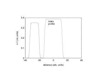
Figure 1: Incident field (amplitude arbitrary) just before it enters the linear medium.

The gradient that has been applied to the index has also been applied to the permeability as a matter of convenience. Figure 2 presents a time-domain numerical solution of the wave equation at a later time $t_{1}$ when the refracted field $\tilde{A}_{t}(z)=({\bf\tilde{A}}(z,t_{1})\cdot{\bf\tilde{A}}^{*}(z,t_{1}))^{1/2}$ is entirely inside the medium.

Figure 2: Refracted field entirely within the linear medium.

The pulse has not propagated as far as it would have propagated in the vacuum due to the reduced speed of light $c/n$ in the material. In addition, the spatial extent of the refracted pulse in the medium is $w_{t}=w_{i}/n$ in terms of the width $w_{i}$ of the incidence pulse due to the reduced speed of light. As shown in Fig. 2, the amplitude of the refracted field is ${\tilde{A}}_{t}=\sqrt{{\mu}/{n}}{\tilde{A}}_{i}$, that is, the amplitude of the incident field scaled by $\sqrt{\mu/n}$. Using these relations we can construct the temporally invariant quantity

$$U_{total}=\int_{\sigma}\frac{n}{2}\left(\sqrt{\frac{n}{\mu}}\frac{\omega_{d}}{c}\tilde{A}\right)\left(\sqrt{\frac{n}{\mu}}\frac{\omega_{d}}{c}\tilde{A}\right)^{*}dv$$ (13)

and note that $U_{total}$ is conserved when the integration is performed over a region $V$ that contains all of the electromagnetic field that is present in the system. In that case, the region of integration $V$ is extended to all space, $\sigma$. The pulse that is used in Fig. 1 has a generally rectangular shape in order to facilitate a graphical interpretation of pulse width and integration under the field envelope. It can be shown by additional numerical solutions of the wave equation that the relations described above are quite general in terms of the permeability and the refractive index, as well as the shape and amplitude of a quasimonochromatic field.

For a stationary linear medium, the total energy is the electromagnetic energy. Although a material may possess many forms of energy, we intend total energy to mean all of the energy that impacts the dynamics or electrodynamics of the model system with the specified conditions. In particular, kinetic energy is excepted by the requirement for the material to remain stationary. We assume that the electromagnetic energy density for a stationary simple linear medium is

$$\rho_{e}=\frac{1}{2}\frac{1}{\mu}\left(n^{2}{\bf E}^{2}+{\bf B}^{2}\right)dv\,,$$ (14)

as inferred from the Poynting theorem. Again extending the region of integration $V$ that contains all fields present to integration over all space $\sigma$, the electromagnetic energy,

$$U_{e}=\int_{\sigma}\rho_{e}dv=\int_{\sigma}\frac{1}{2}\frac{1}{\mu}\left(n^{2}{\bf E}^{2}+{\bf B}^{2}\right)dv\,,$$ (15)

is the total energy of the closed system containing a stationary simple linear medium illuminated by a quasimonochromatic pulse of light. Using Eqs. (9) and (10) to eliminate the electric and magnetic fields in Eq. (15), we obtain the energy formula

$$U_{e}=\int_{\sigma}\frac{1}{2}\frac{1}{\mu}\left(\left(\frac{n}{c}\frac{\partial{\bf A}}{\partial t}\right)^{2}+(\nabla\times{\bf A})^{2}\right)dv\,.$$ (16)

Employing the expression for the vector potential in terms of slowly varying envelope functions and carrier waves, Eq. (12), results in

$$U_{e}=\int_{\sigma}\frac{\omega_{d}^{2}n^{2}}{4\mu c^{2}}\left(\tilde{A}\tilde{A}^{*}-\tilde{A}^{2}e^{-2i(\omega_{d}-k_{d}z)t}+c.c.\right)dv\,.$$ (17)

Applying a time average allows the double frequency terms to be neglected and shows the equality of Eqs. (13) and (16),

$$U_{e}=\int_{\sigma}\frac{\omega_{d}^{2}n^{2}}{2\mu c^{2}}|\tilde{A}|^{2}dv=U_{total}\,.$$ (18)

We have theoretical confirmation that our numerical $U_{total}$, Eq. (13), is the total energy of the system and that it is conserved. More importantly, we have an interpretation of the continuum electrodynamic energy formula, Eq. (15), in term of what happens to the shape and amplitude of the electromagnetic field as it propagates into the medium.

In the first half of the last century, there was an ongoing theoretical and experimental effort devoted to determining the correct description of the momentum of light propagating through a linear medium BIPfei ; BIMilBoy ; BIKemp ; BIBaxL ; BIBarL . At various times, the issue was resolved in favor of the Abraham momentum

$${\bf G}_{A}=\int_{\sigma}\frac{{\bf E}\times{\bf H}}{c}dv$$ (19)

and at other times the momentum was found to be the Minkowski momentum

$${\bf G}_{M}=\int_{\sigma}\frac{{\bf D}\times{\bf B}}{c}dv\,.$$ (20)

Since Penfield and Haus BIPenHau showed, in 1967, that neither the Abraham momentum nor the Minkowski momentum is the total momentum, the resolution of the Abraham–Minkowski controversy has been that the momentum for an arbitrary or unspecified field subsystem must be supplemented by an appropriate material momentum to obtain the total momentum BIPfei ; BIMilBoy ; BIKemp ; BIBaxL ; BIBarL ; BIPenHau ; BIMikura ; BINelson ; BIBPRL ; BIObuk ; BIGord ; BIBrev ; BIKran . Then, it must be demonstrated that the total momentum, so constructed, is actually conserved in a thermodynamically closed system, as that is usually not the case. Although continuity equations are often called conservation laws, the derivation of a result that has the outward appearance of a continuity equation is not sufficient to prove conservation.

Given the arbitrariness of the field momentum and the model dependence of the material momentum that go into a construction of the total momentum, the only convincing way to determine the total momentum is by the application of conservation principles. Then conservation of the total energy is all that is needed to prove that the total momentum BIGord ; BICB ; BICB2 ; BISPIE

$${\bf G}_{total}=\int_{\sigma}\frac{1}{\mu}\frac{n{\bf E}\times{\bf B}}{c}dv=\int_{\sigma}\frac{n{\bf E}\times{\bf H}}{c}dv$$ (21)

is conserved in our closed system. In the limit of slowly varying plane waves, we have the conserved vector quantity

$${\bf G}_{total}=\int_{\sigma}\frac{\omega_{d}^{2}n^{2}}{2\mu c^{3}}|\tilde{A}|^{2}dv{\bf e}_{\bf k}=\frac{U_{total}}{c}{\bf e}_{\bf k}$$ (22)

that is equal to the conserved total energy, Eq. (18), divided by a constant factor of $c$ and multiplied by a unit vector ${\bf e}_{\bf k}$. In addition to being conserved, the total momentum, Eq. (21), is unique. There can be no other non-trivial conserved macroscopic momentum in terms of the vector product of electric and magnetic fields in our model system because these would contain different combinations of the material properties. The momentum formula, Eq. (21), was originally derived for a dielectric in 1973 by Gordon BIGord who combined the Abraham momentum for the field with a material momentum that was obtained from integrating the Lorentz force on the microscopic constituents of matter. Although, Gordon’s derivation is incorrect and incomplete BImicro , conservation of the total momentum is definitive and the Gordon momentum is uniquely conserved in a thermodynamically closed continuum electrodynamic system containing a stationary simple linear medium. The Gordon momentum is actually composed of the momentum of the electric, magnetic, and polarization fields BImicro . We can associate the polarization field with the material, but apart from a semantic artifice, the momentum, like the energy, is entirely electromagnetic in nature.

III Total Energy–Momentum Tensor

A tensor is a very special mathematical object and a total energy–momentum tensor is subject to even more stringent conditions. Any four continuity equations, or equations that have the outward appearance of being continuity equations, can be combined using linear algebra to form a matrix differential equation. Hence, the proliferation of matrices that have been purported to be the energy–momentum tensor for a system containing an electromagnetic pulse and a linear medium. In this section, we construct the unique total energy–momentum tensor and the tensor continuity equation for a stationary simple linear medium using the conservation, symmetry, trace, and divergence conditions that must be satisfied.

For an unimpeded (force-free) flow, conservation of the components of the total four-momentum $(U,{\bf G})$ BILL

$$U=\int_{\sigma}T^{00}dv$$ (23)

$$G^{i}=\frac{1}{c}\int_{\sigma}T^{i0}dv$$ (24)

uniquely determines the first column of the total energy–momentum tensor. We use the convention that Roman indices from the middle of the alphabet, like $i$, run from 1 to 3 and Greek indices belong to $\{0,1,2,3\}$. As in Section II, the region of integration has been extended to all-space, $\sigma$. Conservation of angular momentum in a closed system imposes the diagonal symmetry condition BILL

$$T^{\alpha\beta}=T^{\beta\alpha}$$ (25)

and uniquely determines the first row of the total energy–momentum tensor based on the uniqueness of the first column. Applying the conservation of the total energy and total momentum, we can construct the total energy–momentum tensor

$$T^{\alpha\beta}=$$

$$\left[\begin{matrix}(n^{2}{\bf E}^{2}+{\bf B}^{2})/(2\mu)&(n{\bf E}\times{\bf H})_{1}&(n{\bf E}\times{\bf H})_{2}&(n{\bf E}\times{\bf H})_{3}\cr(n{\bf E}\times{\bf H})_{1}&W_{11}&W_{12}&W_{13}\cr(n{\bf E}\times{\bf H})_{2}&W_{21}&W_{22}&W_{23}\cr(n{\bf E}\times{\bf H})_{3}&W_{31}&W_{32}&W_{33}\cr\end{matrix}\right]$$ (26)

from elements that are obtained by equating Eq. (15) to Eq. (23) and equating Eq. (21) to Eq. (24). The elements of the Maxwell stress-tensor $W$ are yet to be specified.

Our approach here is very different from the usual technique of constructing the energy–momentum tensor from the electromagnetic continuity equations. The energy continuity equation is known to be given by Poynting’s theorem

$$\frac{1}{c}\frac{\partial\rho_{e}}{\partial t}+\nabla\cdot\left({\bf E}\times{\bf H}\right)=0\,.$$ (27)

However if we use Poynting’s theorem and the tensor energy continuity law

$$\partial_{\beta}T^{0\beta}=0$$ (28)

to populate the first row of the energy–momentum tensor, then Eq. (24) becomes

$$G^{i}=\frac{1}{c}\int_{\sigma}({\bf E}\times{\bf H})_{i}dv$$ (29)

by symmetry, Eq. (25). This result is contraindicated because

$${\bf G}=\frac{1}{c}\int_{\sigma}\frac{\omega_{d}^{2}n}{2\mu c^{2}}|\tilde{A}|^{2}{\bf e}_{\bf k}dv=\frac{U_{total}}{nc}{\bf e}_{\bf k}$$ (30)

is not temporally invariant as the pulse travels from the vacuum into the medium. The practice has been to ignore the condition that the components of the four-momentum, Eqs. (23) and (24), be conserved and use the components of the Poynting vector, along with the electromagnetic energy density, to populate the first row of the energy–momentum tensor using the tensor energy continuity law, Eq. (28).

We regard the conservation properties of the total energy–momentum tensor as fundamental and these conservation properties conclusively establish Eq. (26) as the form of the energy–momentum tensor. Applying the tensor continuity equation, Eq. (28), to the energy–momentum tensor, Eq. (26), we obtain an energy continuity equation

$$\frac{1}{c}\frac{\partial\rho_{e}}{\partial t}+\nabla\cdot\left(n{\bf E}\times{\bf H}\right)=0$$ (31)

that is inconsistent with the Poynting theorem, Eq. (27). In the limit of slowly varying plane waves, we obtain an obvious contradiction

$$\frac{n^{2}\omega_{d}^{2}}{2\mu c^{3}}\left({\bf\tilde{A}}\frac{\partial{\bf\tilde{A}}^{*}}{\partial t}+c.c.\right)-\frac{n^{3}\omega_{d}^{2}}{2\mu c^{3}}\left({\bf\tilde{A}}\frac{\partial{\bf\tilde{A}}^{*}}{\partial t}+c.c.\right)=0$$ (32)

from the energy continuity equation, Eq. (31).

We have identified the essential contradiction of the Abraham–Minkowski controversy: Absent the uniqueness that accompanies conservation of total energy and total momentum, the components of the first row and column of the energy–momentum tensor are essentially arbitrary thereby rendering the energy–momentum tensor meaningless. Yet, the energy continuity equation that is obtained from the four-divergence of an energy–momentum tensor that is populated with the densities of the conserved energy and momentum quantities is demonstrably false. We are at an impasse with the existing theory that requires two contradictory conditions to be satisfied BISPIE .

The resolution of this contradiction cannot be found within the formal system of continuum electrodynamics as it currently exists. Therefore we make an $ansatz$, based on the reduced speed of light in the medium, $c/n$, that the continuity equations are generated by

$$\bar{\partial}_{\beta}T^{\alpha\beta}=f_{\alpha}\,,$$ (33)

where $\bar{\partial}_{\beta}$ is the material four-divergence operator BICB ; BICB2 ; BISPIE ; BIFinn

$$\bar{\partial}_{\beta}=\left(\frac{n}{c}\frac{\partial}{\partial t},\frac{\partial}{\partial x},\frac{\partial}{\partial y},\frac{\partial}{\partial z}\right)\,.$$ (34)

The continuity equation, Eq. (33), is generalized in a form that allows a source/sink $f_{\alpha}$ of energy and the components of momentum BICB2 . Reference BIxxx provides a solid theoretical justification for the ansatz of Eqs. (33) and (34). Applying the tensor continuity law, Eq. (33), to the energy–momentum tensor, Eq. (26), we obtain the energy continuity equation

$$\frac{n}{c}\frac{\partial\rho_{e}}{\partial t}+\nabla\cdot\left(n{\bf E}\times{\bf H}\right)=f_{0}\,.$$ (35)

Now, let us re-consider the Poynting theorem. We multiply Poynting’s theorem, Eq. (27), by $n$ and use a vector identity to commute the index of refraction with the divergence operator to obtain BICB

$$\frac{n}{c}\frac{\partial\rho_{e}}{\partial t}+\nabla\cdot\left(n{\bf E}\times{\bf H}\right)=\frac{\nabla n}{n}\cdot(n{\bf E}\times{\bf H})\,.$$ (36)

The two energy continuity equations, Eqs. (35) and (36), are equal if we identify the source/sink of energy as

$$f_{0}=\frac{\nabla n}{n}\cdot(n{\bf E}\times{\bf H})\,.$$ (37)

Then an inhomogeneity in the index of refraction, $\nabla n\neq 0$, is associated with work done by the field on the material or work done on the field by the interaction with the material BICB2 . Obviously, the gradient of the index of refraction in our anti-reflection coating must be sufficiently small that the work done is perturbative.

The Poynting’s theorem that is found in Eq. (36) is a mixed second-order vector differential equation. It can be separated into mixed first-order vector differential equations for the macroscopic electric and magnetic fields

$$\frac{n}{c}\frac{\partial{\bf B}}{\partial t}=-\nabla\times n{\bf E}+\frac{\nabla n}{n}\times n{\bf E}$$ (38)

$$\frac{n}{c}\frac{\partial n{\bf E}}{\partial t}=\mu\nabla\times{\bf H}.$$ (39)

The remaining task is to show that the material four-divergence of the energy–momentum tensor is a faithful representation of the electromagnetic continuity equations. We multiply Eq. (38) by ${\bf H}$ and multiply Eq. (39) by $n{\bf E}$. The resulting equations are summed to produce an energy continuity equation

$$\frac{n}{c}\frac{\partial\rho_{e}}{\partial t}+\nabla\cdot\left(n{\bf E}\times{\bf H}\right)=\frac{\nabla n}{n}\cdot(n{\bf E}\times{\bf H})$$ (40)

that is precisely the same as Eq. (36). To obtain the total momentum continuity equation, we substitute Eqs. (38) and (39) into the material timelike derivative of the total momentum density

$$\frac{n}{c}\frac{\partial{\bf g}_{total}}{\partial t}=\frac{1}{\mu}\frac{n}{c^{2}}\frac{\partial n{\bf E}}{\partial t}\times{\bf B}+n{\bf E}\times\frac{1}{\mu}\frac{n}{c^{2}}\frac{\partial{\bf B}}{\partial t}\,$$ (41)

where the momentum density ${\bf g}_{total}$ is the integrand of Eq. (21). The momentum continuity equation is

$$\frac{n}{c}\frac{\partial{\bf g}_{total}}{\partial t}=\frac{1}{c\mu}\Bigg{[}(\nabla\times n{\bf E})\times n{\bf E}$$

$$+\mu^{2}(\nabla\times{\bf H})\times{\bf H}+\frac{\nabla n}{n}(n{\bf E})^{2}-\left(n{\bf E}\cdot\frac{\nabla n}{n}\right)n{\bf E}\Bigg{]}.$$ (42)

For a dielectric medium, $\mu=1$, we are done and this case was treated in Refs. BICB ; BICB2 ; BISPIE . However, if $\mu\neq 1$ then the momentum continuity equation, Eq. (42), is not expressible as part of the tensor continuity equation, Eq. (33), without additional transformations.

There is a scientific record of algebraic transformations of the energy and momentum continuity equations. Abraham BIAbr was apparently the first to pursue this approach, deriving a variant form of the continuity equation for the Minkowski momentum in which the time-derivative of the Minkowski momentum is split into the temporal derivative of the Abraham momentum and a fictitious Abraham force. Kinsler, Favaro, and McCall BIKins discuss various transformations of Poynting’s theorem and the resulting differences in the way various physical processes are expressed. Frias and Smolyakov BIFrias did the same for transformations of the momentum continuity equation. It appears to have gone unrecognized, however, that the different expression of physical processes in the electromagnetic continuity equations has to carry over into the Maxwell equations of motion for the macroscopic fields, Eqs. (38) and (39). Specifically, the energy and momentum continuity equations are components of the tensor continuity equation, Eq. (33), and cannot be separately transformed. We could, for example, commute the magnetic permeability with the curl operator in the Maxwell–Ampère Law, Eq. (39), in order to allow the momentum continuity law, Eq. (42) to be expressed in the form of a continuity equation. However, the resulting energy continuity law would run afoul of the uniqueness condition on the elements of the first column of the energy–momentum tensor.

The total energy–momentum tensor, Eq. (26), was constructed using conservation principles and it is inarguably correct as long as the formula for the energy, Eq. (15), is correct. For a linear medium with a full or partial magnetic response, however, we have demonstrated that the continuity equations, Eqs. (40) and (42), that were constructed from the field equations, Eq. (38) and (39), are not consistent with the tensor continuity equation, Eq. (33). Again, we are confronted with a situation of contradiction that we cannot derive our way out of and we must justify a correction based on an analysis of the physical model.

IV The Linear Index of Refraction

Consider a rectangular volume of space $V=Ad$, where $A$ is the cross-sectional area perpendicular to the direction of an incident electromagnetic pulse of radiation in the plane-wave limit. The volume is separated into halves by a thin transparent barrier at $d/2$. Half of the volume is filled with a vapor with refractive index $n_{1}$ and the other half of the volume is filled with a vapor with refractive index $n_{2}$. We define a material variable $\xi_{i}=n_{i}-1$. Then the time that it takes a light pulse to traverse the volume is $(\xi_{1}+\xi_{2})d/(2c)$ greater than the time it takes light to travel the same distance in a vacuum. Note that reflections do not affect the time-of-flight of the pulse, only the amount of light that is transmitted. The time-of-flight of the light pulse does not change when the barrier is removed. The atoms of each vapor are noninteracting and there is no physical process that would affect the time-of-flight of the light pulse as the two species of atoms diffuse into each other. Generalizing to an arbitrary number of components, $s$, the linear refractive index of a mixture of vapors obeys a superposition principle

$$n=1+\sum_{k=1}^{s}\xi_{k}.$$ (43)

As long as the atoms are noninteracting, the superposition principle holds whether the vapors are composed of atoms that behave as electric dipoles, magnetic dipoles, or as a mixture of both. That is,

$$n=1+\sum_{i=1}^{p}\xi_{i}+\sum_{j=1}^{q}\xi_{j}$$ (44)

for $p$ dielectric components and $q$ magnetic components. Then, $n=1+\xi_{e}+\xi_{m}$, where $\xi_{e}=\chi_{e}/2$ is the renormalized electric susceptibility and $\xi_{m}=\chi_{m}/2$ is the renormalized magnetic susceptibility. It should be noted that this is not the first time that the refractive index was derived as a linear superposition of the electric and magnetic dipole densities BIWardWebb . It is also common in the literature to invoke the low-density limit so that $n=1+\xi_{e}+\xi_{m}$ can be used in place of $n=\sqrt{(1+\chi_{e})(1+\chi_{m})}$, Ref. BIGord , for example BImicro . Near-dipole–dipole interactions BIChuck , and other interactions between atoms, require a more detailed and model-dependent treatment that is outside the scope of the current work.

Now that the linear refractive index is truly linear, we can regard the permittivity and permeability as anachronisms. The refractive index carries the material effects and we can eliminate the permeability and permittivity from the equations of motion for the macroscopic fields, Eqs. (38) and (39), such that

$$\frac{n}{c}\frac{\partial{\bf B}}{\partial t}=\nabla\times{\bf\Pi}-\frac{\nabla n}{n}\times{\bf\Pi}$$ (45)

$$\frac{n}{c}\frac{\partial{\bf\Pi}}{\partial t}=-\nabla\times{\bf B}\,,$$ (46)

where ${\bf\Pi}=(n/c)\partial{\bf A}/\partial t$. The equations of motion for the macroscopic fields, Eqs. (45) and (46), can be combined in the usual manner to write an energy continuity equation

$$\frac{n}{c}\frac{\partial}{\partial t}\left[\frac{1}{2}\left({\bf\Pi}^{2}+{\bf B}^{2}\right)\right]+\nabla\cdot\left({\bf B}\times{\bf\Pi}\right)=\frac{\nabla n}{n}\cdot({\bf B}\times{\bf\Pi})$$ (47)

in terms of a total energy density

$$\rho_{total}=\frac{1}{2}\left({\bf\Pi}^{2}+{\bf B}^{2}\right)\,,$$ (48)

a total momentum density

$${\bf g}_{total}=\frac{{\bf B}\times{\bf\Pi}}{c}\,,$$ (49)

and a power density

$$p_{total}=\frac{\nabla n}{n}\cdot({\bf B}\times{\bf\Pi})\,.$$ (50)

Substituting Eqs. (45) and (46) into the material timelike derivative of the total momentum, Eq. (49), the momentum continuity equation becomes

$$\frac{n}{c}\frac{\partial{\bf g}_{total}}{\partial t}+\frac{1}{c}\nabla\cdot{\bf W}=\frac{1}{c}\frac{\nabla n}{n}{\bf\Pi}^{2}\,,$$ (51)

where the Maxwell stress-tensor $W$ is

$$W_{ij}=-\Pi_{i}\Pi_{j}-B_{i}B_{j}+\frac{1}{2}({\bf\Pi}^{2}+{\bf B}^{2})\delta_{ij}\,.$$ (52)

We can construct the total energy–momentum tensor

$$T^{\alpha\beta}=\left[\begin{matrix}({\bf\Pi}^{2}+{\bf B}^{2})/2&({\bf B}\times{\bf\Pi})_{1}&({\bf B}\times{\bf\Pi})_{2}&({\bf B}\times{\bf\Pi})_{3}\cr({\bf B}\times{\bf\Pi})_{1}&W_{11}&W_{12}&W_{13}\cr({\bf B}\times{\bf\Pi})_{2}&W_{21}&W_{22}&W_{23}\cr({\bf B}\times{\bf\Pi})_{3}&W_{31}&W_{32}&W_{33}\cr\end{matrix}\right]$$ (53)

from the homogeneous part of the new electromagnetic continuity equations, Eqs. (47) and (51). The total energy–momentum tensor, Eq. (53), is entirely electromagnetic in character BImicro and there is no need for a supplemental dust energy–momentum tensor for the movement of the material BIPfei . The Maxwell–Ampère Law, Eq. (46), can be written in terms of the vector potential as a wave equation

$$\nabla\times(\nabla\times{\bf A})+\frac{n^{2}}{c^{2}}\frac{\partial^{2}{\bf A}}{\partial t^{2}}=0\,,$$ (54)

without the inhomogeneous part found in Eq. (11). We also correct the electromagnetic, or total, energy, Eq. (15),

$$U_{e}=\int_{\sigma}\rho_{e}dv=\int_{\sigma}\frac{1}{2}\left({\bf\Pi}^{2}+{\bf B}^{2}\right)dv\,,$$ (55)

and the total momentum, Eq. (21),

$${\bf G}_{total}=\int_{\sigma}\frac{{\bf B}\times{\bf\Pi}}{c}dv$$ (56)

using the total energy density, Eq. (48), and the total momentum density, Eq. (49).

The ${\{\bf E}$, ${\bf D}$, ${\bf B}$, ${\bf H}\}$ paradigm of classical continuum electrodynamics is altogether broken. That much was obvious from the conservation of the Gordon form of momentum in Refs. BIGord and BICB , also in Eq. (21). The Abraham and Minkowski momentums are expressible solely in terms of the ${\{\bf E}$, ${\bf D}$, ${\bf B}$, ${\bf H}$} fields, while the Gordon momentum depends on the magnetic field ${\bf B}$ and the peculiar macroscopic field ${\bf\Pi}=-n{\bf E}$. This is likely a contributing factor to the longevity of the Abraham–Minkowski controversy. The macroscopic field equations, Eqs. (45) and (46), depend only on the fields ${\bf\Pi}$ and ${\bf B}$. Consequently, continuum electrodynamics can be reformulated in terms of a single pair of fields $\{{\bf\Pi},{\bf B}\}$ and a single field-strength tensor BIxxx

$$F^{\alpha\beta}=\left[\begin{matrix}0&\Pi_{x}&\Pi_{y}&\Pi_{z}\cr-\Pi_{x}&0&-B_{z}&B_{y}\cr-\Pi_{y}&B_{z}&0&-B_{x}\cr-\Pi_{z}&-B_{y}&B_{x}&0\cr\end{matrix}\right]\,.$$ (57)

Having eliminated $\varepsilon$ and $\mu$, the fields ${\bf\Pi}$ and ${\bf B}$ are measurable in the same units, thereby completing the unification of electricity and magnetism that was begun by Maxwell. The reduction to a single pair of fields and a single field-strength tensor is an exquisite simplification of continuum electrodynamics.

The changes to the theoretical treatment of electromagnetic fields in linear media that have been presented here are stunning and it is customary to propose experiments that would validate unordinary theoretical results. However, the existing experimental record related to the Abraham–Minkowski controversy is an indication of serious technical and conceptual difficulties in the measurement of continuum electrodynamic phenomena related to macroscopic fields inside materials, fields that cannot be measured directly. On the other hand, the renormalization of time $t^{\prime}=t/n$ in a linear medium is relatively easy to measure. An open optical cavity, or free-space stolon, is a clock that ticks once for every round-trip of a light pulse and that ticks more slowly when it is immersed in a dielectric fluid.

V Conclusion

The Maxwell equations are widely recognized as one of the most successful theoretical treatments of our physical world, ever. Then, the persistent inability to adequately address an important issue in a simple continuous linear medium using the macroscopic Maxwell theory should be seriously disturbing. Instead the Abraham–Minkowski controversy has been treated as a tautological curiosity in which some momentum quantity is supplemented by another momentum quantity, as long as the correct total momentum is achieved BIPfei ; BIBarL . In the context of the open systems typically used in the treatment of continuum electrodynamics, the Abraham–Minkowski controversy, which is well-posed as a conservation issue, becomes ill-posed and difficult to treat rigorously BIKran . The resolution of the Abraham–Minkowski dilemma in terms of a self-consistent four-dimensional treatment of continuum electrodynamics in a thermodynamically closed system based on the energy and momentum conservation properties of the total energy–momentum tensor forces us to confront a contradiction in the Maxwell formulation of classical continuum electrodynamics. This contradiction is not a minor issue as it resides at the very heart of the relations between energy and momentum. The contradiction is resolved by constructing a unified version of continuum electrodynamics that is based on establishing consistency between the equations of motion for macroscopic fields, the continuity equations, the energy–momentum tensor, and the field-strength tensor for a thermodynamically closed system with complete equations of motion. Like Newtonian dynamics is a low-velocity limit of Einstein relativity, Maxwellian macroscopic electrodynamics must be realizable in some limit of the more complete theory. Indeed that is the case. Natural materials are predominately dielectric or predominately magnetic. Fields inside materials cannot be measured directly and the two theories yield identical observable results for a given refractive index $n$ for materials that can be characterized as either dielectric or magnetic, but not as a combination of both.

References

- (1) M. Abraham, Rend. Circ. Mat. Palermo 28, 1 (1909).
- (2) H. Minkowski, Natches. Ged. Wiss. Göttingen 53 (1908).
- (3) R. N. C. Pfeifer, T. A. Nieminen, N. R. Heckenberg, and H. Rubinsztein-Dunlop, Rev. Mod. Phys. 79, 1197–1216 (2007).
- (4) P. W. Milonni and R. W. Boyd, Adv. Opt. Photon. 2, 519–553 (2010).
- (5) B. A. Kemp, J. Appl. Phys. 109, 111101 (2011).
- (6) C. Baxter and R. Loudon, J. Mod. Opt. 57, 830–842 (2010).
- (7) S. M. Barnett and R. Loudon, Phil. Trans. R. Soc. A 368, 927–939 (2010).
- (8) P. Penfield, Jr. and H. A. Haus, Electrodynamics of Moving Media (MIT Press, 1967).
- (9) Z. Mikura, Phys. Rev. A 13, 2265–2275 (1976).
- (10) D. F. Nelson, Phys. Rev. A 44, 3985–3996 (1991).
- (11) S. M. Barnett, Phys. Rev. Lett. 104, 070401 (2010).
- (12) Y. N. Obukhov, Ann. Phys. (Berlin) 17, 830 (2008).
- (13) J. P. Gordon, Phys. Rev. A 8, 14-21 (1973).
- (14) I. Brevik, Phys. Rep 52, 133-201 (1979).
- (15) M. Kranyš, Int. J. Engng. Sci. 20, 1193-1213 (1982).
- (16) M. E. Crenshaw, Annals of Physics 338, 97-106 (2013).
- (17) M. E. Crenshaw and T. B. Bahder, Opt. Commun. 284, 2460-2465 (2011).
- (18) M. E. Crenshaw and T. B. Bahder, Opt. Commun. 285, 5180-5183 (2012).
- (19) M. E. Crenshaw, Proc. SPIE 8458, Optical Trapping and Optical Micromanipulation IX, 845804 (2012).
- (20) F. Ravndal, arxiv:0804.4013v3 (2008).
- (21) P. Kinsler, A. Favaro, and M. W. McCall, European J. Phys. 30, 983 (2009).
- (22) W. Frias and A. I. Smolyakov, Phys. Rev. E 85, 046606 (2012).
- (23) W. Rindler, Introduction to Special Relativity (Oxford, New York, 1982).
- (24) L. D. Landau and E. M. Lifshitz, Electrodynamics of Continuous Media (Addison-Wesley, Reading, 1960).
- (25) M. E. Crenshaw, arxiv:1303.1412 (2013).
- (26) D. W. Ward, K. A. Nelson, and K. J. Webb, New J. Phys. 7, 213 (2005).
- (27) Y. Ben-Aryeh, C. M. Bowden, and J. C. Englund, Phys. Rev. A 34, 3917 (1986).