Untangling two systems of noncrossing curves

Abstract

We consider two systems $(\alpha_{1},\ldots,\alpha_{m})$ and $(\beta_{1},\ldots,\beta_{n})$ of simple curves drawn on a compact two-dimensional surface ${\mathcal{M}}$ with boundary.

Each $\alpha_{i}$ and each $\beta_{j}$ is either an arc meeting the boundary of ${\mathcal{M}}$ at its two endpoints, or a closed curve. The $\alpha_{i}$ are pairwise disjoint except for possibly sharing endpoints, and similarly for the $\beta_{j}$. We want to “untangle” the $\beta_{j}$ from the $\alpha_{i}$ by a self-homeomorphism of ${\mathcal{M}}$; more precisely, we seek a homeomorphism $\varphi\colon{\mathcal{M}}\to{\mathcal{M}}$ fixing the boundary of ${\mathcal{M}}$ pointwise such that the total number of crossings of the $\alpha_{i}$ with the $\varphi(\beta_{j})$ is as small as possible. This problem is motivated by an application in the algorithmic theory of embeddings and $3$-manifolds.

We prove that if ${\mathcal{M}}$ is planar, i.e., a sphere with $h\geq 0$ boundary components (“holes”), then $O(mn)$ crossings can be achieved (independently of $h$), which is asymptotically tight, as an easy lower bound shows.

In general, for an arbitrary (orientable or nonorientable) surface ${\mathcal{M}}$ with $h$ holes and of (orientable or nonorientable) genus $g\geq 0$, we obtain an $O((m+n)^{4})$ upper bound, again independent of $h$ and $g$.

The proofs rely, among other things, on a result concerning simultaneous planar drawings of graphs by Erten and Kobourov.

1 Introduction

Let ${\mathcal{M}}$ be a surface, by which we mean a two-dimensional compact manifold with (possibly empty) boundary $\partial{\mathcal{M}}$. (Unless stated otherwise, we work with connected surfaces.)

By the classification theorem for surfaces, if ${\mathcal{M}}$ is orientable, then ${\mathcal{M}}$ is homeomorphic to a sphere with $h\geq 0$ holes and $g\geq 0$ attached handles (see Fig. 2); the number $g$ is also called the orientable genus of ${\mathcal{M}}$. If ${\mathcal{M}}$ is nonorientable, then it is homeomorphic to a sphere with $h\geq 0$ holes and with $g\geq 0$ cross-caps; in this case, the integer $g$ is known as the nonorientable genus of ${\mathcal{M}}$. In the sequel, the word “genus” will mean orientable genus for orientable surfaces and nonorientable genus for nonorientable surfaces.

We will consider curves in ${\mathcal{M}}$ that are properly embedded, i.e., every curve is either a simple arc meeting the boundary $\partial{\mathcal{M}}$ exactly at its two endpoints, or a simple closed curve avoiding $\partial{\mathcal{M}}$. An almost-disjoint system of curves in ${\mathcal{M}}$ is a collection $A=(\alpha_{1},\ldots,\alpha_{m})$ of curves that are pairwise disjoint except for possibly sharing endpoints.

In this paper we consider the following problem: We are given two almost-disjoint systems $A=(\alpha_{1},\ldots,\alpha_{m})$ and $B=(\beta_{1},\ldots,\beta_{n})$ of curves in ${\mathcal{M}}$, where the curves of $B$ intersect those of $A$ possibly very many times, as in Fig. 1(a). We would like to “redraw” the curves of $B$ in such a way that they intersect those of $A$ as little as possible.

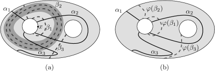
Figure 1: Systems $A$ and $B$ of curves on a surface ${\mathcal{M}}$, with $g=0$ and $h=3$ (a), and a re-drawing of $B$ via a $\partial$-automorphism $\varphi$ (composed of an isotopy and a Dehn twist of the darkly shaded annular region, see below) so that the number of intersections is reduced (b).

We consider re-drawings only in a restricted sense, namely, induced by $\partial$-automorphisms of ${\mathcal{M}}$, where a $\partial$-automorphism is a homeomorphism $\varphi\colon{\mathcal{M}}\to{\mathcal{M}}$ that fixes the boundary $\partial{\mathcal{M}}$ pointwise. Thus, given the $\alpha_{i}$ and the $\beta_{j}$, we are looking for a $\partial$-automorphism $\varphi$ such that the number of intersections (crossings) between $\alpha_{1},\ldots,\alpha_{m}$ and $\varphi(\beta_{1}),\ldots,\varphi(\beta_{n})$ is as small as possible (where sharing endpoints does not count). We call this minimum number of crossings achievable through any choice of $\varphi$ the entanglement number of the two systems $A$ and $B$.

In the orientable case, let $f_{g,h}(m,n)$ denote the maximum entanglement number of any two systems $A=(\alpha_{1},\ldots,\alpha_{m})$ and $B=(\beta_{1},\ldots,\beta_{n})$ of almost-disjoint curves on an orientable surface of genus $g$ with $h$ holes. Analogously, we define $\hat{f}_{g,h}(m,n)$ as the maximum entanglement number of any two systems $A$ and $B$ of $m$ and $n$ curves, respectively, on a nonorientable surface of genus $g$ with $h$ holes. It is easy to see that $f$ and $\hat{f}$ are nondecreasing in $m$ and $n$, which we will often use in the sequel.

To give the reader some intuition about the problem, let us illustrate which re-drawings are possible with a $\partial$-automorphism and which are not. In the example of Fig. 1, it is clear that the two crossings of $\beta_{3}$ with $\alpha_{3}$ can be avoided by sliding $\beta_{3}$ aside. It is perhaps less obvious that the crossings of $\beta_{2}$ can also be eliminated: To picture a suitable $\partial$-automorphism, one can think of an annular region in the interior of ${\mathcal{M}}$, shaded darkly in Fig. 1 (a), that surrounds the left hole and $\beta_{1}$ and contains most of the spiral formed by $\beta_{2}$. Then we cut ${\mathcal{M}}$ along the outer boundary of that annular region, twist the region two times (so that the spiral is unwound), and then we glue the outer boundary back. Here is an example of a single twist of an annulus; straight-line curves on the left are transformed to spirals on the right (this kind of homeomorphism is often called a Dehn twist).

On the other hand, it is impossible to eliminate the crossings of $\beta_{1}$ or $\beta_{3}$ with $\alpha_{2}$ by a $\partial$-automorphism. For example, we cannot re-route $\beta_{1}$ to go around the right hole and thus avoid $\alpha_{2}$, since this re-drawing is not induced by any $\partial$-automorphism $\varphi$: indeed, $\beta_{1}$ separates the point $x$ on the boundary of left hole from the right hole, whereas $\alpha_{2}$ does not separate them; therefore, the curve $\alpha_{2}$ has to intersect $\varphi(\beta_{1})$ at least twice, once when it leaves the component containing $x$ and once when it returns to this component.

A rather special case of our problem, with $m=n=1$ and only closed curves, was already considered by Lickorish [Lic62], who showed that the intersection of a pair of simple closed curves can be simplified via Dehn twists (and thus a $\partial$-automorphism) so that they meet at most twice (also see Stillwell [Sti80]). The case with $m=1$, $n$ arbitrary, only closed curves, and ${\mathcal{M}}$ possibly nonorientable was proposed in 2010 as a Mathoverflow question [Huy10] by T. Huynh. In an answer A. Putman proposes an approach via the “change of coordinates principle” (see, e.g., [FM11, Sec. 1.3]), which relies on the classification of 2-dimensional surfaces—we will also use it at some points in our argument.

The results. A natural idea for bounding $f_{g,h}(m,n)$ and $\hat{f}_{g,h}(m,n)$ is to proceed by induction, employing the change of coordinates principle mentioned above. This does indeed lead to finite bounds, but the various induction schemes we have tried always led to bounds at least exponential in one of $m,n$. Independently of our work, Geelen, Huynh, and Richter [GHR13] also recently proved bounds of this kind; see the discussion below. Partially influenced by the results on exponentially many intersections in representations of string graphs and similar objects (see [KM91, SSŠ03]), we first suspected that an exponential behavior might be unavoidable. Then, however, we found, using a very different approach, that polynomial bounds actually do hold.

For planar ${\mathcal{M}}$, i.e., $g=0$, we obtain an asymptotically tight bound:

Theorem 1.1.

For planar ${\mathcal{M}}$, we have $f_{0,h}(m,n)=O(mn),$ independent of $h$.

Here and in the sequel, the constants implicit in the $O$-notation are absolute, independent of $g$ and $h$.

A simple example providing a lower bound of $2mn$ is obtained, e.g., by replicating $\alpha_{2}$ in Fig. 1 $m$ times and $\beta_{1}$ $n$ times. We currently have no example forcing more than $2mn$ intersections.

In general, we obtain the following bounds:

Theorem 1.2.

1. For the orientable case,

   $$f_{g,h}(m,n)=O((m+n)^{4}).$$

2. For the nonorientable case,

   $$\hat{f}_{g,h}(m,n)=O((m+n)^{4}).$$

Both parts of Theorems 1.2 are derived from the planar case, Theorem 1.1. In the orientable case, we use the following results on genus reduction. For a convenient notation, let us set $L=\max(m,n)$.

Proposition 1.3 (Orientable genus reductions).

1. For $g>L$, we have

   $$f_{g,h}(m,n)\leq f_{L,g+h-L}(m,n).$$

2. $f_{g,h}(m,n)\leq f_{0,h+1}(cg(m+g),cg(n+g))$ for a suitable constant $c>0$.

To derive Theorem 1.2 (i), for $g>L$, we use Proposition 1.3(i), then (ii), and then the planar bound: $f_{g,h}(m,n)\leq f_{L,g+h-L}(m,n)\leq f_{0,g+h+1-L}(2cL^{2},2cL^{2})=O(L^{4})$. For $g\leq L$, we omit the first step.

In the nonorientable case, Theorem 1.2 (ii) is derived in two steps. First, analogous to Proposition 1.3 (i), we have the following reduction:

Proposition 1.4 (Nonorientable genus reduction).

For $g>4L+2$, we have

$$\hat{f}_{g,h}(m,n)\leq\hat{f}_{g^{\prime},h^{\prime}}(m,n),$$

where $g^{\prime}=4L+2-(g\operatorname{mod}2)$ and $h^{\prime}=h+\lceil g/2\rceil-2L-1$.

The second step is a reduction to the orientable case.

Proposition 1.5 (Orientability reduction).

There is a constant $c$ such that

$$\hat{f}_{g,h}(m,n)\leq f_{\lfloor(g-1)/2\rfloor,h+1+(g\operatorname{mod}2)}(c(g+m),c(g+n)).$$

Now we can derive Theorem 1.2 (ii). We set $L:=\max(m,n)$. For $g>4L+2$, we use Proposition 1.4, then Proposition 1.5. We also use monotonicity of the entanglement numbers in $m$ and $n$. We obtain $\hat{f}_{g,h}(m,n)\leq\hat{f}_{4L+2-(g\operatorname{mod}2),\vartheta_{1}(g,h,m,n)}(m,n)\leq f_{2L,\vartheta_{2}(g,h,m,n)}(6cL,6cL)$ where $\vartheta_{1}$ and $\vartheta_{2}$ are functions that, for simplicity, we do not evaluate explicitly. Then we use Proposition 1.3 and the planar bound, Theorem 1.1, to obtain an $O(L^{4})$ bound similarly as in the orientable case. For $g\leq 4L+2$, we omit the first step. Table 1 summarizes the proof of Theorem 1.2.

  1. For a planar surface, temporarily remove the holes not incident to any $\alpha_{i}$ or $\beta_{j}$, and contract the remaining “active” holes, augment the resulting planar graphs to make them 3-connected. Make a simultaneous plane drawing of the resulting planar graphs $G_{1}$ and $G_{2}$ with every edge of $G_{1}$ intersecting every edge of $G_{2}$ at most $O(1)$ times. Decontract the active holes and put the remaining holes back into appropriate faces (Theorem 1.1; Section 2). 2. If the genus is larger than $c(m+n)$, find handles or cross-caps avoided by the $\alpha_{i}$ and $\beta_{j}$, temporarily remove them, untangle the $\alpha_{i}$ and $\beta_{j}$, and put the handles or cross-caps back (Propositions 1.3 (i) and 1.4; Section 3). 3. If the surface is nonorientable, make it orientable by cutting along a suitable curve that intersects the $\alpha_{i}$ and $\beta_{j}$ at most $O(m+n)$ times, untangle the resulting pieces of the $\alpha_{i}$ and $\beta_{j}$, and glue back (Proposition 1.5; Section 5). 4. Make the surface planar by cutting along a suitable system of curves (canonical system of loops), untangle the resulting pieces of the $\alpha_{i}$ and $\beta_{j}$, and glue back (Proposition 1.3 (ii); Section 4).

Table 1: A summary of the proof.

Motivation. We were led to the question concerning untangling curves on surfaces while working on a project on $3$-manifolds and embeddings. Specifically, we are interested in an algorithm for the following problem: given a $3$-manifold $M$ with boundary, does $M$ embed in the $3$-sphere? A special case of this problem, with the boundary of $M$ a torus, was solved in [JS03]. The general version of the problem is motivated, in turn, by the question of algorithmically testing the embeddability of a $2$-dimensional simplicial complex in $\mathbb{R}^{3}$; see [MTW11].

Very recently, we showed that these embeddability problems are algorithmically decidable, see [MSTW14]. For the proof, we use the following upper bound on $f_{g,h}(m,n)$ and $\hat{f}_{g,h}(m,n)$, which we state here as a separate corollary in the specific form used in [MSTW14], for convenience of reference.

Corollary 1.6.

Both $f_{g,h}(m,n)$ and $\hat{f}_{g,h}(m,n)$ are bounded from above by $K(g)mn$, where $K(g)$ is a computable function of $g$, independent of $h$ (in fact, $K(g)=O(g^{4})$).

Proof.

By Thm. 1.1, for planar ${\mathcal{M}}$, we have $f_{0,h}=O(mn)$. By Prop. 1.3 (ii), in case of an orientable surface of arbitrary genus, $f_{g,h}(m,n)\leq f_{0,h+1}(cg(m+g),cg(n+g))=O(g^{2}(m+g)(n+g))=O(g^{4}mn)$. For the nonorientable case, Prop. 1.5 gives $\hat{f}_{g,h}(m,n)\leq f_{\lfloor(g-1)/2\rfloor,h+1+(g\mod 2)}(c(m+g),c(n+g))=O(g^{4}mn)$ as well. ∎

Independently of the application to embeddability, we consider the problem investigated in this paper interesting in itself and contributing to a better understanding of combinatorial properties of curves on surfaces.

As mentioned above, the question studied in the present paper has also been investigated independently by Geelen, Huynh, and Richter [GHR13], with a rather different and very strong motivation stemming from the theory of graph minors, namely the question of obtaining explicit upper bounds for the graph minor algorithms of Robertson and Seymour. Phrased in the language of the present paper, Geelen et al. [GHR13, Theorem 2.1] show that $f_{g,h}(m,n)$ and $\hat{f}_{g,h}(m,n)$ are both bounded by $n3^{m}$, but only under the assumption that ${\mathcal{M}}\setminus(\beta_{1}\cup\cdots\cup\beta_{n})$ is connected.

Further work. We suspect that the bound in Theorem 1.2 should also be $O(mn)$. The possible weak point of the current proof is the reduction in Proposition 1.3(ii), from genus comparable to $m+n$ to the planar case.

This reduction uses a result of the following kind: given a graph $G$ with $n$ edges embedded on a compact $2$-manifold ${\mathcal{M}}$ of genus $g$ (without boundary), one can construct a system of curves on ${\mathcal{M}}$ such that cutting ${\mathcal{M}}$ along these curves yields one or several planar surfaces, and at the same time, the curves have a bounded number of crossings with the edges of $G$ (see Section 4). Concretely, we use a result of Lazarus et al. [LPVV01], where the system of curves is of a special kind, forming a canonical system of loops. (This result is in fact essentially due to Vegter and Yap [VY90]; however, the formulation in [LPVV01] is more convenient for our purposes.) Their result is asymptotically optimal for a canonical system of loops, but it may be possible to improve it for other systems of curves. This and similar questions have been studied in the literature, mostly in algorithmic context (see, e.g., [CM07, DFHT05, Col03, Col12] for some of the relevant works), but we haven’t found any existing result superior to that of Lazarus et al. for our purposes.

2 Planar Surfaces

In this section we prove Theorem 1.1. In the proof we use the following basic fact (see, e.g., [MT01]).

Lemma 2.1.

If $G$ is a maximal planar simple graph (a triangulation), then for every two planar drawings of $G$ in $S^{2}$ there is an automorphism $\psi$ of $S^{2}$ converting one of the drawings into the other (and preserving the labeling of the vertices and edges). Moreover, if an edge $e$ is drawn by the same arc in both of the drawings, w.l.o.g. we may assume that $\psi$ fixes this arc pointwise.

Let us introduce the following piece of terminology. Let $G$ be as in the lemma, and let $D_{G}$, $D^{\prime}_{G}$ be two planar drawings of $G$. We say that $D_{G},D^{\prime}_{G}$ are directly equivalent if there is an orientation-preserving automorphism of $S^{2}$ mapping $D_{G}$ to $D^{\prime}_{G}$, and we call $D_{G},D^{\prime}_{G}$ mirror-equivalent if there is an orientation-reversing automorphism of $S^{2}$ converting $D_{G}$ into $D^{\prime}_{G}$.

We will also rely on a result concerning simultaneous planar embeddings; see [BKR12]. Let $V$ be a vertex set and let $G_{1}=(V,E_{1})$ and $G_{2}=(V,E_{2})$ be two planar graphs on $V$. A planar drawing $D_{G_{1}}$ of $G_{1}$ and a planar drawing $D_{G_{2}}$ of $G_{2}$ are said to form a simultaneous embedding of $G_{1}$ and $G_{2}$ if each vertex $v\in V$ is represented by the same point in the plane in both $D_{G_{1}}$ and $D_{G_{2}}$ (in particular any edge drawn in $D_{G_{1}}$ may intersect any edge drawn in $D_{G_{2}}$).

We note that $G_{1}$ and $G_{2}$ may have common edges, but they are not required to be drawn in the same way in $D_{G_{1}}$ and in $D_{G_{2}}$. If this requirement is added, one speaks of a simultaneous embedding with fixed edges. There are pairs of planar graphs known that do not admit any simultaneous embedding with fixed edges (and consequently, no simultaneous straight-line embedding). An important step in our approach is very similar to the proof of the following result.

Theorem 2.2 (Erten and Kobourov [EK05]).

Every two planar graphs $G_{1}=(V,E_{1})$ and $G_{2}=(V,E_{2})$ admit a simultaneous embedding in which every edge is drawn as a polygonal line with at most $3$ bends.

We will need the following result, which follows easily from the proof given in [EK05]. For the reader’s convenience, instead of just pointing out the necessary modifications, we present a full proof.

Theorem 2.3.

Every two planar graphs $G_{1}=(V,E_{1})$ and $G_{2}=(V,E_{2})$ admit a simultaneous, piecewise linear embedding in which each edge of $G_{1}$ and each edge of $G_{2}$ intersect at least once and at most $C$ times, for a suitable constant $C$.

In addition, if both $G_{1}$ and $G_{2}$ are maximal planar graphs, let us fix a planar drawing $D^{\prime}_{G_{1}}$ of $G_{1}$ and a planar drawing $D^{\prime}_{G_{2}}$ of $G_{2}$. The planar drawing of $G_{1}$ in the simultaneous embedding can be required to be either directly equivalent to $D^{\prime}_{G_{1}}$, or mirror-equivalent to it, and similarly for the drawing of $G_{2}$ (each of the four combinations can be prescribed).

Proof.

For the beginning, we assume that both graphs are Hamiltonian. Later on, we will drop this assumption.

Let $v_{1},v_{2},\dots,v_{n}$ be the order of the vertices as they appear on (some) Hamiltonian cycle $H_{1}$ of $G_{1}$. Since the vertex set $V$ is common for $G_{1}$ and $G_{2}$, there is a permutation $\pi\in S(n)$ such that $v_{\pi(1)},\dots,v_{\pi(n)}$ is the order of the vertices as they appear on some Hamiltonian cycle $H_{2}$ of $G_{2}$.

We draw the vertex $v_{i}$ in the grid point $p_{i}=(i,\pi(i))$, $i=1,2,\ldots,n$. Let $S$ be the square $[1,n]\times[1,n]$. A bispiked curve is an $x$-monotone polygonal curve with two bends such that it starts inside $S$; the first bend is above $S$, the second bend is below $S$ and it finishes in $S$ again.

The $n-1$ edges $v_{i}v_{i+1}$, of $H_{1}$, $i=1,2,\ldots,n-1$, are drawn as bispiked curves starting in $p_{i}$ and finishing in $p_{i+1}$. In order to distinguish edges and their drawings, we denote these bispiked curves by $c(i,i+1)$.

Similarly, we draw the edges $v_{\pi(i)}v_{\pi(i+1)}$ of $H_{2}$, $i=1,2,\ldots,n-1$, as $y$-monotone analogs of bispiked curves, where the first bend is on the left of $S$ and the second is on the right of $S$; here is an example:

We continue only with description of how to draw $G_{1}$; $G_{2}$ is drawn analogously with the grid rotated by $90$ degrees.

Let $D^{\prime}_{G_{1}}$ be a planar drawing of $G_{1}$. Every edge from $E_{1}$ that is not contained in $H_{1}$ is drawn either inside $D^{\prime}_{H_{1}}$ or outside. Thus, we split $E_{1}\setminus E(H_{1})$ into two sets $E^{\prime}_{1}$ and $E^{\prime\prime}_{1}$.

Let $P_{0}$ be the polygonal path obtained by concatenation of the curves $c(1,2)$, $c(2,3),\dots$, $c(n-1,n)$. Now our task is to draw the edges of $E^{\prime}_{1}\cup\{v_{1}v_{n}\}$ as bispiked curves, all above $P_{0}$, and then the edges of $E^{\prime\prime}_{1}$ below $P_{0}$.

We start with $E^{\prime}_{1}$ and we draw edges from it one by one, in a suitably chosen order, while keeping the following properties.

1. Every edge $v_{i}v_{j}$, where $i<j$, is drawn as a bispiked curve $c(i,j)$ starting in $p_{i}$ and ending in $p_{j}$.

2. The $x$-coordinate of the second bend of $c(i,j)$ belongs to the interval $[j-1,j]$.

3. The polygonal curve $P_{k}$ that we see from above after drawing the $k$th edge is obtained as a concatenation of some curves $c(1,i_{1}),c(i_{1},i_{2}),\dots,c(i_{\ell},n)$.

Here is an illustration; the square $S$ is deformed for the purposes of the drawing:

Initially, before drawing the first edge, the properties are obviously satisfied.

Let us assume that we have already drawn $k-1$ edges of $E^{\prime}_{1}$, and let us focus on drawing the $k$th edge. Let $e=v_{i}v_{j}\in E^{\prime}_{1}$ be an edge that is not yet drawn and such that all edges below $e$ are already drawn, where “below $e$” means all edges $v_{i^{\prime}}v_{j^{\prime}}\in E^{\prime}_{1}$ with $i\leq i^{\prime}<j^{\prime}\leq j$, $(i,j)\neq(i^{\prime},j^{\prime})$. (This choice ensures that we will draw all edges of $E^{\prime}_{1}$.)

Since $D^{\prime}_{G_{1}}$ is a planar drawing, we know that there is no edge $v_{i^{\prime}}v_{j^{\prime}}\in E^{\prime}_{1}$ with $i<i^{\prime}<j<j^{\prime}$ or $i^{\prime}<i<j^{\prime}<j$, and so the points $p_{i}$ and $p_{j}$ have to belong to $P_{k-1}$. The subpath $P^{\prime}$ of $P_{k-1}$ between $p_{i}$ and $p_{j}$ is the concatenation of curves $c(i,\alpha_{1}),c(\alpha_{1},\alpha_{2}),\dots,c(\alpha_{s},j)$ as in the inductive assumptions. In particular, the $x$-coordinate of the second bend $b^{*}$ of $c(\alpha_{s},j)$ belongs to the interval $[j-1,j]$. We draw $c(i,j)$ as follows: The second bend of $c(i,j)$ is slightly above $b^{*}$ but still below the square $S$. The first bend of $S$ is sufficiently high above $S$ (with the $x$-coordinate somewhere between $i$ and $j-1$) so that the resulting bispiked curve $c(i,j)$ does not intersect $P_{k-1}$. The properties (P1) and (P2) are obviously satisfied by the construction. For (P3), the path $P_{k}$ is obtained from $P_{k-1}$ by replacing $P^{\prime}$ with $c(i,j)$.

After drawing the edges of $E^{\prime}_{1}$, we draw $v_{1}v_{n}$ in the same way. Then we draw the edges of $E^{\prime\prime}_{1}$ in a similar manner as those of $E^{\prime}_{1}$, this time as bispiked curves below $P_{0}$. This finishes the construction for Hamiltonian graphs.

Now we describe how to adjust this construction for non-Hamiltonian graphs, in the spirit of [EK05].

First we add edges to $G_{1}$ and $G_{2}$ so that they become planar triangulations. This step does not affect the construction at all, except that we remove these edges in the final drawing.

Next, we subdivide some of the edges of $G_{i}$ with dummy vertices. Moreover, we attach two new extra edges to each dummy vertex, as in the following illustration:

By choosing the subdivided edges suitably, one can obtain a $4$-connected, and thus Hamiltonian, graph; see [EK05, Proof of Theorem 2] for details (this idea previously comes from [KW02]). An important property of this construction is that each edge of $G_{i}$ is subdivided at most once.

In this way, we obtain new Hamiltonian graphs $G^{\prime}_{1}$ and $G^{\prime}_{2}$, for which we want to construct a simultaneous drawing as in the first part of the proof. A little catch is that $G^{\prime}_{1}$ and $G^{\prime}_{2}$ do not have same vertex sets, but this is easy to fix. Let $d_{i}$ be the number of dummy vertices of $G^{\prime}_{i}$, $i=1,2$, and say that $d_{1}\geq d_{2}$. We pair the $d_{2}$ dummy vertices of $G^{\prime}_{2}$ with some of the dummy vertices of $G^{\prime}_{1}$. Then we iteratively add $d_{1}-d_{2}$ new triangles to $G^{\prime}_{2}$, attaching each of them to an edge of a Hamiltonian cycle. This operation keeps Hamiltonicity and introduces $d_{1}-d_{2}$ new vertices, which can be matched with the remaining $d_{1}-d_{2}$ dummy vertices in $G^{\prime}_{1}$.

After drawing resulting graphs, we remove all extra dummy vertices and extra edges added while introducing dummy vertices. An original edge $e$ that was subdivided by a dummy vertex is now drawn as a concatenation of two bispiked curves. Therefore, each edge is drawn with at most $5$ bends.

Two edges with 5 bends each may in general have at most 36 intersections, but in our case, there can be at most 25 intersections, since the union of the two segments before and after a dummy vertex is both $x$-monotone and $y$-monotone.

Because of the bispiked drawing of all edges, it is also clear that every edge of $G_{1}$ crosses every edge of $G_{2}$ at least once.

Finally, the requirements on directly equivalent or mirror-equivalent drawings can easily be fulfilled by interchanging the role of top and bottom in the drawing of $G_{1}$ or left and right in the drawing of $G_{2}$. Theorem 2.3 is proved. ∎

Proof of Theorem 1.1..

Let a planar surface ${\mathcal{M}}$ and the curves $\alpha_{1},\ldots,\alpha_{m}$, $\beta_{1},\ldots,\beta_{n}$ be given; we assume that ${\mathcal{M}}$ is a subset of $S^{2}$. Furthermore; by eventually applying some $\partial$-automorphism moving the curves $\beta_{j}$, we can assume that for every $i$ and $j$ the curves $\alpha_{i}$ and $\beta_{j}$ meet on the boundary in the endpoints or in the interior transversally and in a finite number of points. From this we construct a set $V$ of $O(m+n)$ vertices in $S^{2}$ and planar drawings $D_{G_{1}}$ and $D_{G_{2}}$ of two simple graphs $G_{1}=(V,E_{1})$ and ${G_{2}}=(V,E_{2})$ in $S^{2}$, as follows.

1. We put all endpoints of the $\alpha_{i}$ and of the $\beta_{j}$ into $V$ (note that some of them can be shared).

2. We choose a new vertex in the interior of each $\alpha_{i}$ and each $\beta_{j}$, or two distinct vertices if $\alpha_{i}$ or $\beta_{j}$ is a loop with a single endpoint, or three vertices if $\alpha_{i}$ or $\beta_{j}$ is a closed curve, and we add all of these vertices to $V$. These new vertices are all distinct and do not lie on any curves other than where they were placed.

3. If the boundary of a hole in ${\mathcal{M}}$ already contains a vertex introduced so far, we add more vertices so that it contains at least $3$ vertices of $V$. This finishes the construction of $V$.

4. To define the edge set $E_{1}=E(G_{1})$ and the planar drawing $D_{G_{1}}$, we take the portions of the curves $\alpha_{1},\ldots,\alpha_{m}$ between consecutive vertices of $V$ as edges of $E_{1}$. Similarly, we make the arcs of the boundaries of the holes into edges in $E_{1}$; these will be called the hole edges. By the choice of the vertex set $V$ above, this yields a simple plane graph.

5. Then we add new edges to $E_{1}$ so that we obtain a drawing $D_{G_{1}}$ in $S^{2}$ of a maximal planar simple graph $G_{1}$ (i.e., a triangulation) on the vertex set $V$. While choosing these edges, we make sure that all holes containing no vertices of $G$ lie in faces of $D_{G_{1}}$ adjacent to some of the $\alpha_{i}$. New edges drawn in the interior of a hole are also called hole edges.

6. We construct ${G_{2}}=(V,E_{2})$ and $D_{G_{2}}$ analogously, using the curves $\beta_{1},\ldots,\beta_{n}$. We make sure that all hole edges are common to $G_{1}$ and ${G_{2}}$.

After this construction, each hole of ${\mathcal{M}}$ contains either no vertex of $V$ on its boundary or at least three vertices. In the former case, we speak of an inner hole, and in the latter case, of a subdivided hole. A face $f$ of $D_{G_{1}}$ or $D_{G_{2}}$ is a non-hole face if it is not contained in a subdivided hole. An inner hole $H$ has its signature, which is a pair $(f_{1},f_{2})$, where $f_{1}$ is the unique non-hole face of $D_{G_{1}}$ containing $H$, and $f_{2}$ is the unique non-hole face of $D_{G_{2}}$ containing $H$. By the construction, each $f_{1}$ appearing in a signature is adjacent to some $\alpha_{i}$, and each $f_{2}$ is adjacent to some $\beta_{j}$.

In the following claim, we will consider different drawings $D^{\prime}_{G_{1}}$ and $D^{\prime}_{G_{2}}$ for $G_{1}$ and ${G_{2}}$. By Lemma 2.1, the faces of $D_{G_{1}}$ are in one-to-one correspondence with the faces of $D^{\prime}_{G_{1}}$. For a face $f_{1}$ of $D_{G_{1}}$, we denote the corresponding face by $f^{\prime}_{1}$, and similarly for a face $f_{2}$ of $D_{G_{2}}$ and $f^{\prime}_{2}$.

Claim 2.4.

The graphs $G_{1}$ and ${G_{2}}$ as above have planar drawings $D^{\prime}_{G_{1}}$ and $D^{\prime}_{G_{2}}$, respectively, that form a simultaneous embedding in which each edge of $G_{1}$ crosses each edge of $G_{2}$ at most $C$ times, for a suitable constant $C$; moreover, $D^{\prime}_{G_{1}}$ is directly equivalent to $D_{G_{1}}$; $D^{\prime}_{G_{2}}$ is directly equivalent to $D_{G_{2}}$; all hole edges are drawn in the same way in $D^{\prime}_{G_{1}}$ and $D^{\prime}_{G_{2}}$; and whenever $(f_{1},f_{2})$ is a signature of an inner hole, the interior of the intersection $f^{\prime}_{1}\cap f^{\prime}_{2}$ is nonempty.

We postpone the proof of Claim 2.4, and we first finish the proof of Theorem 1.1 assuming this claim.

For each inner hole $H$ with signature $(f_{1},f_{2})$, we introduce a closed disk $B_{H}$ in the interior of $f^{\prime}_{1}\cap f^{\prime}_{2}$. We require that these disks are pairwise disjoint. In sequel, we consider holes as subsets of $S^{2}$ homeomorphic to closed disks (in particular, a hole $H$ intersects ${\mathcal{M}}$ in $\partial H$).

Claim 2.5.

There is an orientation-preserving automorphism $\varphi_{1}$ of $S^{2}$ transforming every inner hole $H$ to $B_{H}$ and $D_{G_{1}}$ to $D^{\prime}_{G_{1}}$.

Proof.

Using Lemma 2.1 again, there is an orientation-preserving automorphism $\psi_{1}$ transforming $D_{G_{1}}$ into $D^{\prime}_{G_{1}}$ (since $D_{G_{1}}$ and $D^{\prime}_{G_{1}}$ are directly equivalent).

Let $f_{1}$ be a face of $D_{G_{1}}$. The interior of $f^{\prime}_{1}$ contains images $\psi_{1}(H)$ of all holes $H$ with signature $(f_{1},\cdot)$, and it also contains the disks $B_{H}$ for these holes. Therefore, there is a boundary- and orientation-preserving automorphism of $f^{\prime}_{1}$ that maps each $\psi_{1}(H)$ to $B_{H}$.

By composing these automorphisms on every $f^{\prime}_{1}$ separately, we have an orientation-preserving automorphism $\psi_{2}$ fixing $D^{\prime}_{G_{1}}$ and transforming each $\psi_{1}(H)$ to $B_{H}$. The required automorphism is $\varphi_{1}=\psi_{2}\psi_{1}$. ∎

Claim 2.6.

There is an orientation-preserving automorphism $\varphi_{2}$ of $S^{2}$ that fixes hole edges (of subdivided holes), fixes $B_{H}$ for every inner hole $H$, and transforms $\varphi_{1}(D_{G_{2}})$ to $D^{\prime}_{G_{2}}$.

Proof.

By Lemma 2.1 there is an orientation-preserving automorphism $\psi_{3}$ of $S^{2}$ that fixes hole edges and transforms $\varphi_{1}(D_{G_{2}})$ to $D^{\prime}_{G_{2}}$.

If an inner hole $H$ has a signature $(\cdot,f_{2})$, then both $\psi_{3}(B_{H})$ and $B_{H}$ belong to the interior of $f^{\prime}_{2}$. Therefore, as in the proof of the previous claim, there is an orientation-preserving homeomorphism $\psi_{4}$ that fixes $D^{\prime}_{G_{2}}$ and transforms $\psi_{3}(B_{H})$ to $B_{H}$. We can even require that $\psi_{4}\psi_{3}$ is identical on $B_{H}$. We set $\varphi_{2}:=\psi_{4}\psi_{3}$. ∎

To finish the proof of Theorem 1.1, we set $\varphi=\varphi_{1}^{-1}\varphi_{2}\varphi_{1}$. We need that $\varphi$ fixes the holes (inner or subdivided) and that $\alpha_{1},\dots,\alpha_{m}$ and $\varphi(\beta_{1}),\dots,\varphi_{1}(\beta_{m})$ have $O(mn)$ intersections. It is routine to check all the properties:

If $H$ is a hole (inner or subdivided), then $\varphi_{2}$ fixes $\partial\varphi_{1}(H)$. Therefore, $\varphi$ also restricts to a $\partial$-automorphism of ${\mathcal{M}}$.

The collections of curves $\alpha_{1},\dots,\alpha_{m}$ and $\varphi(\beta_{1}),\dots,(\beta_{m})$ have same intersection properties as the collections $\varphi_{1}(\alpha_{1}),\dots$, $\varphi_{1}(\alpha_{m})$ and $\varphi_{2}(\varphi_{1}(\beta_{1})),\dots$, $\varphi_{2}(\varphi_{1}(\beta_{m}))$. Since each $\alpha_{i}$ and each $\beta_{j}$ was subdivided at most three times in the construction, by Claims 2.4, 2.5, and 2.6, these collections have at most $O(mn)$ intersections. The proof of the theorem is finished, except for Claim 2.4. ∎

Proof of Claim 2.4..

Given $G_{1}$ and ${G_{2}}$, we form auxiliary planar graphs $\tilde{G}_{1}$ and $\tilde{G}_{2}$ on a vertex set $\tilde{V}$ by contracting all hole edges and removing the resulting loops and multiple edges. We note that a loop cannot arise from an edge that was a part of some $\alpha_{i}$ or $\beta_{j}$.

Then we consider planar drawings $D_{\tilde{G}_{1}}$ and $D_{\tilde{G}_{2}}$ forming a simultaneous embedding as in Theorem 2.3, with each edge of $\tilde{G}_{1}$ crossing each edge of $\tilde{G}_{2}$ at least once and most a constant number of times.

Let $v_{H}\in\tilde{V}$ be the vertex obtained by contracting the hole edges on the boundary of a hole $H$. Since the drawings $D_{\tilde{G}_{1}}$ and $D_{\tilde{G}_{2}}$ are piecewise linear, in a sufficiently small neighborhood of $v_{H}$ the edges are drawn as radial segments.

We would like to replace $v_{H}$ by a small circle and thus turn the drawings $D_{\tilde{G}_{1}}$, $D_{\tilde{G}_{2}}$ into the required drawings $D^{\prime}_{G_{1}}$, $D^{\prime}_{G_{2}}$. But a potential problem is that the edges in $D_{\tilde{G}_{1}}$, $D_{\tilde{G}_{2}}$ may enter $v_{H}$ in a wrong cyclic order.

We claim that the edges in $D_{\tilde{G}_{1}}$ entering $v_{H}$ have the same cyclic ordering around $v_{H}$ as the corresponding edges around the hole $H$ in the drawing $D_{G_{1}}$. Indeed, by contracting the hole edges in the drawing $D_{G_{1}}$, we obtain a planar drawing $D^{*}_{\tilde{G}_{1}}$ of $\tilde{G}_{1}$ in which the cyclic order around $v_{H}$ is the same as the cyclic order around $H$ in $D_{G_{1}}$ Since $\tilde{G}_{1}$ was obtained by edge contractions from a maximal planar graph, it is maximal as well (since an edge contraction cannot create a non-triangular face), and its drawing is unique up to an automorphism of $S^{2}$ (Lemma 2.1). Hence the cyclic ordering of edges around $v_{H}$ in $D_{\tilde{G}_{1}}$ and in $D^{*}_{\tilde{G}_{1}}$ is either the same (if $D_{\tilde{G}_{1}}$ and $D^{*}_{\tilde{G}_{1}}$ are directly equivalent), or reverse (if $D_{\tilde{G}_{1}}$ and $D^{*}_{\tilde{G}_{1}}$ are mirror-equivalent). However, Theorem 2.3 allows us to choose the drawing $D_{\tilde{G}_{1}}$ so that it is directly equivalent to $D^{*}_{\tilde{G}_{1}}$, and then the cyclic orderings coincide. A similar consideration applies for the other graph $G_{2}$.

The edges of $D_{\tilde{G}_{1}}$ may still be placed to wrong positions among the edges in $D_{\tilde{G}_{2}}$, but this can be rectified at the price of at most one extra crossing for every pair of edges entering $v_{H}$, as the following picture indicates (the numbering specifies the cyclic order of the edges around $H$ in $D_{G_{1}}\cup D_{G_{2}}$):

It remains to draw the edges of $G_{1}$ and $G_{2}$ that became loops or multiple edges after the contraction of the hole edges. Loops can be drawn along the circumference of the hole, and multiple edges are drawn very close to the corresponding single edge.

In this way, every edge of $G_{1}$ still has at most a constant number of intersections with every edge of $G_{2}$, and every two such edges intersect at least once unless at least one of them became a loop after the contraction. Consequently, whenever $(f_{1},f_{2})$ is a signature of an inner hole, the corresponding faces $f_{1}^{\prime}$ and $f_{2}^{\prime}$ intersect. This finishes the proof. ∎

3 Reducing the Genus to $O(m+n)$

In this section we prove Proposition 1.3(i) as well as Proposition 1.4. We begin with several definitions.

3.1 Cutting Along Curves

Let ${\mathcal{M}}$ be an (orientable or nonorientable) surface with boundary. By $h({\mathcal{M}})$ we denote the number of holes in ${\mathcal{M}}$ and by $g({\mathcal{M}})$ we denote the (orientable or nonorientable) genus of ${\mathcal{M}}$.

Now let $\delta$ be a properly embedded curve in ${\mathcal{M}}$ (i.e., either a simple closed curve that avoids the boundary $\partial{\mathcal{M}}$, or a simple arc whose endpoints lie on $\partial{\mathcal{M}}$). The curve $\delta$ is called separating if ${\mathcal{M}}\setminus\delta$ has two components. Otherwise, $\delta$ is non-separating.

We denote by ${\mathcal{M}}_{\langle\delta\rangle}$ the (possibly disconnected) surface obtained by cutting ${\mathcal{M}}$ along $\delta$. If $\delta$ is non-separating, then ${\mathcal{M}}_{\langle\delta\rangle}$ is connected. Otherwise, ${\mathcal{M}}_{\langle\delta\rangle}$ has two components, which we denote by ${\mathcal{M}}_{\langle\delta\rangle}^{1}$ and ${\mathcal{M}}_{\langle\delta\rangle}^{2}$.

Now we recall basic properties of the Euler characteristic of a surface. Given a triangulated surface ${\mathcal{M}}$, the Euler characteristic $\chi({\mathcal{M}})$ is defined as the number of vertices plus number of triangles minus the number of edges in the triangulation. It is well known that the Euler characteristic is a topological invariant and equals $2-2g({\mathcal{M}})-h({\mathcal{M}})$ if ${\mathcal{M}}$ is orientable, and $2-g({\mathcal{M}})-h({\mathcal{M}})$ if ${\mathcal{M}}$ is nonorientable.

To work simultaneously with orientable and nonorientable surfaces, it is also convenient to define the Euler genus of ${\mathcal{M}}$ as $g_{e}({\mathcal{M}}):=2-\chi({\mathcal{M}})-h({\mathcal{M}})$. That is, $g_{e}({\mathcal{M}})=g({\mathcal{M}})$ if ${\mathcal{M}}$ is nonorientable, and $g_{e}({\mathcal{M}})=2g({\mathcal{M}})$ if ${\mathcal{M}}$ is orientable.

We have the following relations for the Euler characteristic:

	$\delta$ is non-separating	$\delta$ is separating
$\delta$ is a closed curve	$\chi({\mathcal{M}})=\chi({\mathcal{M}}_{\langle\delta\rangle})$	$\chi({\mathcal{M}})=\chi({\mathcal{M}}_{\langle\delta\rangle}^{1})+\chi({\mathcal{M}}_{\langle\delta\rangle}^{2})$
$\delta$ is an arc	$\chi({\mathcal{M}})=\chi({\mathcal{M}}_{\langle\delta\rangle})-1$	$\chi({\mathcal{M}})=\chi({\mathcal{M}}_{\langle\delta\rangle}^{1})+\chi({\mathcal{M}}_{\langle\delta\rangle}^{2})-1$

The relations above also allow us to relate the genus of ${\mathcal{M}}$ and the genus of the surface(s) obtained after a cutting.

Let us call a closed curve $\delta$ in ${\mathcal{M}}$ two-sided if a small closed neighborhood of $\delta$ is homeomorphic to the annulus $S^{1}\times[0,1]$; otherwise, $\delta$ is one-sided (and a small closed neighborhood of $\delta$ is a Möbius band). Note that every orientable surface contains only two-sided closed curves.

Lemma 3.1.

We have the following relations for genera:

1. If ${\mathcal{N}}$ is orientable, then

   $$g({\mathcal{M}})=\left\{\begin{array}[]{ll}g({\mathcal{M}}_{\langle\delta\rangle}^{1})+g({\mathcal{M}}_{\langle\delta\rangle}^{2})&\mbox{if $\delta$ is separating};\\ g({\mathcal{M}}_{\langle\delta\rangle})&\mbox{if $\delta$ is a non-separating arc connecting}\\ &\mbox{two different boundary components};\\ g({\mathcal{M}}_{\langle\delta\rangle})+1&\mbox{if $\delta$ is a non-separating closed curve, or}\\ &\mbox{a non-separating arc with both endpoints}\\ &\mbox{in a single boundary component.}\\ \end{array}\right.$$

2. If ${\mathcal{N}}$ is orientable or nonorientable, then

   $$g_{e}({\mathcal{M}})=\left\{\begin{array}[]{ll}g_{e}({\mathcal{M}}_{\langle\delta\rangle}^{1})+g_{e}({\mathcal{M}}_{\langle\delta\rangle}^{2})&\mbox{if $\delta$ is separating};\\ g_{e}({\mathcal{M}}_{\langle\delta\rangle})&\mbox{if $\delta$ is a non-separating arc connecting}\\ &\mbox{two different boundary components};\\ g_{e}({\mathcal{M}}_{\langle\delta\rangle})+1&\mbox{if $\delta$ is a non-separating one-sided closed curve}\\ g_{e}({\mathcal{M}}_{\langle\delta\rangle})+2&\mbox{if $\delta$ is a non-separating arc with both endpoints}\\ &\mbox{in a single boundary component, or}\\ &\mbox{a non-separating two-sided closed curve.}\par\end{array}\right.$$

Note that $(b)$ implies $(a)$. However, it is still convenient to state $(a)$ separately.

Proof.

A simple case analysis yields the following relations for the numbers of holes:

$$h({\mathcal{M}})=\left\{\begin{array}[]{ll}h({\mathcal{M}}_{\langle\delta\rangle}^{1})+h({\mathcal{M}}_{\langle\delta\rangle}^{2})-2&\mbox{if $\delta$ is a separating closed curve};\\ h({\mathcal{M}}_{\langle\delta\rangle})-2&\mbox{if $\delta$ is a two-sided non-separating closed curve};\\ h({\mathcal{M}}_{\langle\delta\rangle})-1&\mbox{if $\delta$ is a one-sided non-separating closed curve};\\ h({\mathcal{M}}_{\langle\delta\rangle}^{1})+h({\mathcal{M}}_{\langle\delta\rangle}^{2})-1&\mbox{if $\delta$ is a separating arc};\\ h({\mathcal{M}}_{\langle\delta\rangle})+1&\mbox{if $\delta$ is a non-separating arc connecting}\\ &\mbox{two different boundary components};\\ h({\mathcal{M}}_{\langle\delta\rangle})-1&\mbox{if $\delta$ is a non-separating arc with both}\\ &\mbox{endpoints in a single boundary component.}\\ \end{array}\right.$$

The proof now follows by simple computation from the table above the lemma and the relations $\chi({\mathcal{M}})=2-2g({\mathcal{M}})-h({\mathcal{M}})$ if ${\mathcal{M}}$ is orientable and $\chi({\mathcal{M}})=2-g_{e}({\mathcal{M}})-h({\mathcal{M}})$ if ${\mathcal{M}}$ is orientable or nonorientable. ∎

3.2 Orientable Surfaces

Let ${\mathcal{M}}$ be a surface, which may be orientable or nonorientable. A handle-enclosing curve is a separating closed curve $\lambda$ in ${\mathcal{M}}$ that splits ${\mathcal{M}}$ into two components ${\mathcal{M}}_{\langle\lambda\rangle}^{+}$ and ${\mathcal{M}}_{\langle\lambda\rangle}^{-}$ such that ${\mathcal{M}}_{\langle\lambda\rangle}^{-}$ is a torus with hole—that is, an orientable surface of genus $1$ with one boundary hole; here are two ways of looking at it:

A system $L$ of handle-enclosing curves is independent if ${\mathcal{M}}_{\langle\kappa\rangle}^{-}\cap{\mathcal{M}}_{\langle\lambda\rangle}^{-}=\emptyset$ for every two closed curves $\kappa,\lambda\in L$.

First we focus on proving Proposition 1.3 (i). For the remainder of this subsection, all surfaces will be orientable.

For an orientable surface of genus $g$ with $h$ holes, we fix a standard representation of this surface, denoted by ${\mathcal{M}}_{g,h}$. It is obtained by removing interiors of $h$ pairwise disjoint disks $H_{1},\dots,H_{h}$ in the southern hemisphere of $S^{2}$ and by removing interiors of $g$ pairwise disjoint disks $D_{1},\dots,D_{g}$ in the northern hemisphere of $S^{2}$ and then attaching a torus with hole along the boundary of each $D_{i}$; see Fig. 2. Note that $\{\partial D_{i}\}_{i=1}^{g}$ is an independent system of handle-enclosing curves.

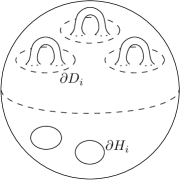
Figure 2: The standard representation ${\mathcal{M}}_{3,2}$.

One of the tools we need (Lemma 3.3) is that if we find handle-enclosing curves in some surface ${\mathcal{M}}$ (of genus $g$ with $h$ holes), then we can find a homeomorphism ${\mathcal{M}}\to{\mathcal{M}}_{g,h}$ mapping these curves to $\partial D_{i}$ extending some given homeomorphism of the boundaries. However, we have to require a technical condition on orientations, to be described next.

Let $\gamma_{1},\dots,\gamma_{h}$ be a collection of the boundary curves of an orientable surface ${\mathcal{M}}$ (of arbitrary genus) with $h$ holes. We assume that $\gamma_{1},\dots,\gamma_{h}$ are also given with orientations. Since ${\mathcal{M}}$ is orientable, it makes sense to speak of whether the orientations of $\gamma_{1},\dots,\gamma_{h}$ are mutually compatible or not: Choose and fix an orientation of ${\mathcal{M}}$. Then we can say for each boundary curve $\gamma_{i}$ whether ${\mathcal{M}}$ lies is on the right-hand side of $\gamma_{i}$ or on the left-hand side (with respect to the chosen orientation of ${\mathcal{M}}$ and the given orientation of $\gamma_{i}$).

Lemma 3.2.

Let ${\mathcal{M}}$ be a planar surface with $h$ holes. Let $\gamma_{1},\dots,\gamma_{h}$ be the boundary curves of ${\mathcal{M}}$ given with compatible orientations. Let $\zeta\colon\partial{\mathcal{M}}\to\partial{\mathcal{M}}_{0,h}$ be a homeomorphism such that the orientations (induced by $\zeta$) of the curves $\zeta(\gamma_{1}),\dots,\zeta(\gamma_{h})$ are compatible. Then $\zeta$ can be extended to a homeomorphism $\bar{\zeta}\colon{\mathcal{M}}\to{\mathcal{M}}_{0,h}$.

The lemma is generally known and the proof is quite straightforward. We keep the proof here for completeness (and for lack of a reference). Similar remark applies to Lemma 3.3 below.

Proof.

If $h=0$, then the claim follows immediately from the classification of surfaces. For $h=1$, an arbitrary homeomorphism $\partial{\mathcal{M}}\to\partial{\mathcal{M}}_{0,h}$ can be extended to a homeomorphism ${\mathcal{M}}\to{\mathcal{M}}_{0,h}$ (between disks) by ‘coning’.

For $h>1$ we prove the lemma by induction in $h$. We connect two (closed) boundary curves $\gamma_{1}$, $\gamma_{2}$ with an arc $\delta$ inside ${\mathcal{M}}$ attached at some points $a$ and $b$ and we also connect $\zeta(\gamma_{1})$ and $\zeta(\gamma_{2})$ inside ${\mathcal{M}}_{0,h}$ with an arc $\delta^{\prime}$ attached at $\zeta(a)$ and $\zeta(b)$. We cut ${\mathcal{M}}$ and ${\mathcal{M}}_{0,h}$ along $\delta$ and $\delta^{\prime}$, obtaining surfaces ${\mathcal{M}}^{*}$ and ${\mathcal{M}}^{*}_{0,h}$ with one hole less.

The holes $\gamma_{3},\dots,\gamma_{h}$ are kept in ${\mathcal{M}}^{*}$, while the holes $\gamma_{1}$ and $\gamma_{2}$ and the arc $\delta$ in ${\mathcal{M}}$ induce a boundary curve $\gamma^{*}$ in ${\mathcal{M}}^{*}$ composed of four arcs $\gamma^{*}_{1}$, $\delta^{*}_{1}$, $\gamma^{*}_{2}$ and $\delta^{*}_{2}$. Since the orientations of $\gamma_{1},\dots,\gamma_{h}$ are compatible, the arcs $\gamma_{1}^{*}$ and $\gamma_{2}^{*}$ are concurrently oriented as subarcs of $\gamma^{*}$, and they induce an orientation of $\gamma^{*}$ still compatible with $\gamma_{3},\dots,\gamma_{h}$.

Similarly, we obtain an orientation on the new hole $\gamma^{\prime*}$ in ${\mathcal{M}}^{*}_{0,h}$. We can also extend $\zeta$ so that $\zeta(\gamma^{*})=\zeta(\gamma^{\prime*})$ (running along $\delta^{*}_{1}$ and $\delta^{*}_{2}$ with same speed). By induction, there is a homeomorphism $\bar{\zeta}^{*}\colon{\mathcal{M}}^{*}\to{\mathcal{M}}^{*}_{0,h}$, and the resulting $\bar{\zeta}$ is obtained by gluing ${\mathcal{M}}^{*}$ and ${\mathcal{M}}^{*}_{0,h}$ back to ${\mathcal{M}}$ and ${\mathcal{M}}_{0,h}$. ∎

Lemma 3.3.

Let $(\lambda_{1},\dots,\lambda_{s})$ be an independent system of handle-enclosing curves in a surface ${\mathcal{M}}$ of genus $g$ with $h$ holes, $s\leq g$. Let $\{\gamma_{i}\}_{i=1}^{h}$ be the system of the boundary curves of the holes in ${\mathcal{M}}$. Then there is a homeomorphism $\psi\colon{\mathcal{M}}\rightarrow{\mathcal{M}}_{g,h}$ such that $\psi(\gamma_{i})=\partial H_{i}$, $i=1,2,\ldots,h$, and $\psi(\lambda_{i})=\partial D_{i}$, $i=1,2,\ldots,s$. Moreover, $\psi$ can be prescribed on the $\gamma_{i}$, assuming that it preserves compatible orientations.

Proof.

First we remark that we can assume that $s=g$. If $s<g$, we can extend $(\lambda_{1},\dots,\lambda_{s})$ to an independent system of handle-enclosing of size $g$: We cut away each torus with hole ${\mathcal{M}}^{-}_{\langle\lambda_{i}\rangle}$, obtaining a surface of genus $g-s$ homeomorphic to ${\mathcal{M}}_{g-s,h+s}$. Then we can find an independent system of $g-s$ handle-enclosing loops in this surface. In sequel, we assume $s=g$.

Let us cut ${\mathcal{M}}$ along the curves $\lambda_{1},\ldots,\lambda_{s}$. It decomposes into a collection $T_{1},\ldots,T_{g}$, where each $T_{i}$ is a torus with hole (with $\partial T_{i}=\lambda_{i}$), and one planar surface ${\mathcal{P}}$ with $g+h$ holes (the boundary curves of ${\mathcal{P}}$ are the $\lambda_{i}$ and the $\gamma_{i}$). In particular, ${\mathcal{M}}$ decomposes into the same collection of surfaces (up to a homeomorphism) as ${\mathcal{M}}_{g,h}$ when cut along $\partial D_{i}$. Let ${\mathcal{P}}^{\prime}$ be the planar surface in this decomposition of ${\mathcal{M}}_{g,h}$.

As we assume in the lemma, $\psi$ can be prescribed on some closed curves of $\partial{\mathcal{P}}$ while preserving compatible orientations. It can also be extended so that it maps each $\lambda_{i}$ to $\partial D_{i}$, while preserving compatible orientations between ${\mathcal{P}}$ and ${\mathcal{P}}^{\prime}$. Then we have, by Lemma 3.2, a homeomorphism between ${\mathcal{P}}$ and ${\mathcal{P}}^{\prime}$ extending $\psi$.

Finally, this homeomorphism can also be extended to all the $T_{i}$, one by one. Note that preserving the orientations is not an issue in this case since the torus with hole admits an automorphism reversing the orientation of the boundary curve. ∎

We state the following corollary of Lemma 3.3, which will be useful in Section 5.

Corollary 3.4.

Let ${\mathcal{M}}_{1}$ and ${\mathcal{M}}_{2}$ be two orientable surfaces of genus $g$ with $h$ holes. Let $\zeta\colon\partial{\mathcal{M}}_{1}\to\partial{\mathcal{M}}_{2}$ be a homeomorphism of the boundaries that preserves compatible orientations. Then $\zeta$ extends to a homeomorphism $\psi$ of ${\mathcal{M}}_{1}$ and ${\mathcal{M}}_{2}$.

Proof.

We find an arbitrary homeomorphism $\zeta_{1}\colon\partial{\mathcal{M}}_{1}\to\partial{\mathcal{M}}_{g,h}$ that preserves compatible orientations. Then the homeomorphism $\zeta_{2}\colon\partial{\mathcal{M}}_{2}\to\partial{\mathcal{M}}_{g,h}$ defined as $\zeta_{2}=\zeta_{1}\zeta^{-1}$ preserves compatible orientations as well. Using Lemma 3.3 (with $s=0$), we obtain extensions $\psi_{1}\colon{\mathcal{M}}_{1}\to{\mathcal{M}}_{g,h}$ and $\psi_{2}\colon{\mathcal{M}}_{2}\to{\mathcal{M}}_{g,h}$. Then $\psi:=\psi^{-1}_{2}\psi_{1}$ is the required homeomorphism. ∎

Lemma 3.5.

Let ${\mathcal{M}}$ be a surface of genus $g$ with $h$ holes. Let $(\delta_{1},\dots,\delta_{n})$ be an almost disjoint system of curves on ${\mathcal{M}}$. Then there is an independent system of $s\geq g-n$ handle-enclosing curves $\lambda_{1},\dots,\lambda_{s}$ such that each of the tori with hole ${\mathcal{M}}^{-}_{\langle\lambda_{j}\rangle}$ is disjoint from $\bigcup_{i=1}^{n}\delta_{i}$.

Proof.

Let us cut ${\mathcal{M}}$ along $\{\delta_{i}\}_{i=1}^{n}$ obtaining several components ${\mathcal{M}}_{1},\dots,{\mathcal{M}}_{q}$. If we cut along the curves one by one, we see that Lemma 3.1(a) implies

$$g({\mathcal{M}}_{1})+\cdots+g({\mathcal{M}}_{q})\geq g({\mathcal{M}})-n.$$

In each ${\mathcal{M}}_{k}$ we find an independent system of $g({\mathcal{M}}_{k})$ handle-enclosing curves (this can be done by transforming ${\mathcal{M}}_{k}$ into the standard representation). The union of these independent systems yields a system as in the lemma. ∎

Proof of Proposition 1.3(i).

Let ${\mathcal{M}}$ be a surface of genus $g$ with $h$ holes. Let $A=(\alpha_{1},\ldots,\alpha_{m})$ and $B=(\beta_{1},\ldots,\beta_{n})$ be two almost disjoint systems of curves in ${\mathcal{M}}$.

Our task is to find a $\partial$-automorphism $\varphi$ of ${\mathcal{M}}$ such that the number of crossings between $\alpha_{1},\dots,\alpha_{m}$ and $\varphi(\beta_{1}),\dots,\varphi(\beta_{n})$ is at most $f_{g-s,h+s}(m,n)$, where $s:=\min(g-m,g-n)$. (Let us recall that we assume that $g>m,n$, and therefore $s>0$.)

By Lemma 3.5 there is an independent system of handle-enclosing curves $\lambda_{1,\alpha},\dots,\lambda_{s,\alpha}$ such that the corresponding tori with hole are disjoint from the curves in $A$. Consequently, by Lemma 3.3, we have a homeomorphism $\psi_{\alpha}\colon{\mathcal{M}}\rightarrow{\mathcal{M}}_{g,h}$, extending a fixed homeomorphism $\psi^{\prime}\colon\partial{\mathcal{M}}\rightarrow\partial{\mathcal{M}}_{g,h}$, which preserves compatible orientations and maps each $\lambda_{k,\alpha}$ to $\partial D_{k}$ (using the notation from the definition of a standard representation).

Similarly, we have an independent system of handle-enclosing curves $\lambda_{1,\beta},\dots,\lambda_{s,\beta}$ with the corresponding tori with hole disjoint from the curves in $B$. We also have a homeomorphism $\psi_{\beta}\colon{\mathcal{M}}\rightarrow{\mathcal{M}}_{g,h}$ extending $\psi^{\prime}$ that maps the (closed) curves $\lambda_{k,\beta}$ to $\partial D_{k}$.

Now we have two systems $A^{\prime}=(\psi_{\alpha}(\alpha_{1}),\dots,\psi_{\alpha}(\alpha_{m}))$ and $B^{\prime}=(\psi_{\beta}(\beta_{1}),\dots,\psi_{\beta}(\beta_{m}))$ of curves in ${\mathcal{M}}_{g,h}$ avoiding the tori with hole bounded by the $\partial D_{i}$. Let us remove these tori (only for $i\leq s$) obtaining a new surface ${\mathcal{M}}^{*}$ of genus $g-s$ with $h+s$ holes. We find a $\partial$-automorphism $\varphi^{*}$ of ${\mathcal{M}}^{*}$ such that number of intersections between $A^{\prime}$ and $\varphi^{*}$-images of the curves in $B^{\prime}$ is at most $f_{g-s,h+s}(m,n)$. Since $\varphi^{*}$ fixes the boundary, it can be extended to a $\partial$-automorphism $\varphi_{g,h}$ of ${\mathcal{M}}_{g,h}$ while introducing no new intersections. Finally, $\varphi:=\psi^{-1}_{\alpha}\varphi_{g,h}\psi_{\beta}$ is the required $\partial$-automorphism of ${\mathcal{M}}$. ∎

3.3 Nonorientable Surfaces

The proof of Proposition 1.4 is similar to the previous proof but simpler, since we need not worry about orientations.

Lemma 3.6.

Let ${\mathcal{N}}$ and ${\mathcal{N}}^{\prime}$ be two nonorientable surfaces with the same genus and number of holes. Let $\psi_{0}\colon\partial{\mathcal{N}}\to\partial{\mathcal{N}}^{\prime}$ be a homeomorphism of the boundaries. Then $\psi_{0}$ extends to a homeomorphism $\psi\colon{\mathcal{N}}\to{\mathcal{N}}^{\prime}$.

Proof.

By the classification of surfaces, ${\mathcal{N}}$ and ${\mathcal{N}}^{\prime}$ are homeomorphic. Given two boundary components, there is a self-homeomorphism of ${\mathcal{N}}$ that exchanges these components. Therefore, we know that there is a homeomorphism $\psi_{1}\colon{\mathcal{N}}\to{\mathcal{N}}$ such that for each component $C$ of $\partial{\mathcal{N}}$ the images $\psi_{0}(C)$ and $\psi_{1}(C)$ coincide (as sets). However, if we equip $C$ with an orientation, it might happen that $\psi_{0}(C)$ and $\psi_{1}(C)$ have opposite orientations. In such case, we consider a self-homeomorphism $\psi_{C}$ of ${\mathcal{N}}$ that reverts the orientation of $C$ and fixes all other boundary components. Here is an example of such a self-homeomorphism:

Up to a homeomorphism, we can consider ${\mathcal{N}}$ as a polygon with holes whose edges are identified according to the labels. By moving the middle hole along $\gamma$, we revert its orientation without affecting the other holes.

By gradually composing $\psi_{1}$ with the $\psi_{C}$ for those $C$ on which orientations disagree, we can get a self-homeomorphism of ${\mathcal{N}}$ such that $\psi_{0}(C)$ and $\psi_{2}(C)$ have compatible orientations for every $C$. Finally, by a local modification of $\psi_{2}$ at small neighborhood of every $C$ we can get a self-homeomorphism $\psi$ of ${\mathcal{N}}$ that agrees with $\psi_{0}$ on $\partial{\mathcal{N}}$. ∎

Similar to the orientable case, we will use a certain canonical representation ${\mathcal{N}}_{g,h}$ for a nonorientable surface of genus $g$ with $h$ holes. We recall that a cross-cap in a nonorientable surface ${\mathcal{N}}$ is a subset of ${\mathcal{N}}$ which is homeomorphic to a Möbius band. Note that the boundary of a cross-cap is a single closed curve. A standard way of representing a nonorientable surface of genus $g$ with $h$ holes is to remove $h$ disjoint disks from the $2$-sphere and replace other $g$ disjoint disks with cross-caps. However, here it is more convenient to replace all but at most two of the cross-caps by handles: indeed, for $g\geq 3$, a pair of cross-caps can be replaced with a handle (this is sometimes called Dyck’s Theorem, see, e.g., [FW99, Lemma 3]; note that it is essential that at least one cross-cap remain present).

Thus, we can define a convenient representation (as opposed to the standard one mentioned above) ${\mathcal{N}}_{g,h}$ as follows. We again start with the sphere $S^{2}$, and we remove $h$ pairwise disjoint disks $H_{1},\dots,H_{h}$. Then we remove $\lfloor(g-1)/2\rfloor$ more disjoint disks $D_{1},\dots,D_{\lfloor(g-1)/2\rfloor}$ and attach a torus with hole along boundary of each $D_{i}$. Finally, we remove one (for $g$ odd) or two (for $g$ even) extra disks and we attach Möbius bands along these disks. Here is the convenient representation of ${\mathcal{N}}_{6,2}$:

Lemma 3.7.

Let $(\lambda_{1},\dots,\lambda_{s})$ be an independent system of handle-enclosing curves in a nonorientable surface ${\mathcal{N}}$ of genus $g$ with $h$ holes, $s\leq\lfloor(g-1)/2\rfloor$. Let $\{\gamma_{i}\}_{i=1}^{h}$ be the system of the boundary curves of the holes in ${\mathcal{N}}$. Then there is a homeomorphism $\psi\colon{\mathcal{N}}\rightarrow{\mathcal{N}}_{g,h}$ such that $\psi(\gamma_{i})=\partial H_{i}$, $i=1,2,\ldots,h$, and $\psi(\lambda_{i})=\partial D_{i}$, $i=1,2,\ldots,s$. Moreover, $\psi$ can be prescribed on the $\gamma_{i}$.

Proof.

The proof is analogous to that of Lemma 3.3. Let us cut ${\mathcal{N}}$ along the curves $\lambda_{1},\ldots,\lambda_{g}$. It decomposes into a collection $T_{1},\ldots,T_{s}$, where each $T_{i}$ is a torus with hole (with $\partial T_{i}=\lambda_{i}$), and one nonorientable surface $\hat{\mathcal{N}}$ of genus $g-2s$ with $h+s$ holes (the boundary curves of ${\mathcal{N}}$ are the $\lambda_{i}$ and the $\gamma_{i}$). In particular, ${\mathcal{N}}$ decomposes into the same collection of surfaces (up to a homeomorphism) as ${\mathcal{N}}_{g,h}$ when cut along the $\partial D_{i}$. Let ${\mathcal{N}}^{\prime}$ be the nonorientable surface in the decomposition of ${\mathcal{N}}_{g,h}$.

By Lemma 3.6, we have a homeomorphism between $\hat{\mathcal{N}}$ and ${\mathcal{N}}^{\prime}$ extending a given homeomorphism of the boundary curves. This homeomorphism can be also extended to all $T_{i}$, one by one. ∎

Lemma 3.8.

Let ${\mathcal{N}}$ be a nonorientable surface of genus $g$ with $h$ holes. Let $(\delta_{1},\dots,\delta_{n})$ be an almost disjoint system of curves on ${\mathcal{M}}$. Then there is an independent system of $s\geq g/2-2n-1$ handle-enclosing curves $\lambda_{1},\dots,\lambda_{s}$ such that each of the tori with hole ${\mathcal{M}}^{-}_{\langle\lambda_{j}\rangle}$ is disjoint from $\bigcup_{i=1}^{n}\delta_{i}$.

Proof.

Let us cut ${\mathcal{N}}$ along $\{\delta_{i}\}_{i=1}^{n}$, obtaining several components ${\mathcal{M}}_{1},\dots,{\mathcal{M}}_{q}$, $q\leq n+1$ (some of them may be orientable and some nonorientable). Cutting along the curves one by one, we see that Lemma 3.1(b) implies

$$g_{e}({\mathcal{M}}_{1})+\cdots+g_{e}({\mathcal{M}}_{q})\geq g_{e}({\mathcal{M}})-2n.$$

In each ${\mathcal{M}}_{k}$ we find an independent system of at least $(g_{e}({\mathcal{M}}_{k})-2)/2$ handle-enclosing curves. Indeed, if ${\mathcal{M}}_{k}$ is orientable, then we can find even $g_{e}({\mathcal{M}}_{k})/2$ such curves by transforming ${\mathcal{M}}_{k}$ to the standard representation. If ${\mathcal{M}}_{k}$ is nonorientable, then we find at least $(g_{e}({\mathcal{M}}_{k})-2)/2$ such curves by transforming ${\mathcal{M}}_{k}$ to the convenient representation.

The union of these independent systems yields a system as in the lemma (using $g=g_{e}({\mathcal{M}})$ and $q\leq n+1$). ∎

Proof of Proposition 1.4.

The proof is now almost same as for Proposition 1.3(i).

Let ${\mathcal{N}}$ be a nonorientable surface of genus $g$ with $h$ holes. Let $A=(\alpha_{1},\ldots,\alpha_{m})$ and $B=(\beta_{1},\ldots,\beta_{n})$ be two almost disjoint systems of curves in ${\mathcal{N}}$.

Our task is to find a $\partial$-automorphism $\varphi$ of ${\mathcal{N}}$ such that the number of crossings between $\alpha_{1},\dots,\alpha_{m}$ and $\varphi(\beta_{1}),\dots,\varphi(\beta_{n})$ is at most $\hat{f}_{g-2s,h+s}(m,n)$, where $s:=\min(\lceil g/2\rceil-2m-1,\lceil g/2\rceil-2n-1)$. Note that $g-2s=4L+2-(g\operatorname{mod}2)$ and $h+s=h+\lceil g/2\rceil-2L-1$ as required ($L=\max(m,n)$). (Let us also recall that we assume that $g>4L+2$, and so $s>0$.)

By Lemma 3.8 there is an independent system of handle-enclosing curves $\lambda_{1,\alpha},\dots,\lambda_{s,\alpha}$ such that the corresponding tori with hole are disjoint from the curves in $A$. Consequently, by Lemma 3.7, we have a homeomorphism $\psi_{\alpha}\colon{\mathcal{N}}\rightarrow{\mathcal{N}}_{g,h}$, extending a fixed homeomorphism $\psi^{\prime}\colon\partial{\mathcal{N}}\rightarrow\partial{\mathcal{N}}_{g,h}$, which maps each $\lambda_{k,\alpha}$ to $\partial D_{k}$.

Similarly, we have an independent system of handle-enclosing curves $\lambda_{1,\beta},\dots,\lambda_{s,\beta}$ with the corresponding tori with hole disjoint from the curves in $B$. We also have a homeomorphism $\psi_{\beta}\colon{\mathcal{N}}\rightarrow{\mathcal{N}}_{g,h}$ extending $\psi^{\prime}$ that maps the each $\lambda_{k,\beta}$ to $\partial D_{k}$.

Now we have two systems $A^{\prime}=(\psi_{\alpha}(\alpha_{1}),\dots,\psi_{\alpha}(\alpha_{m}))$ and $B^{\prime}=(\psi_{\beta}(\beta_{1}),\dots,\psi_{\beta}(\beta_{m}))$ of curves in ${\mathcal{N}}_{g,h}$ avoiding the tori with hole bounded by the $\partial D_{i}$. Let us remove these tori (only for $i\leq s$) obtaining a new surface ${\mathcal{N}}^{*}$ of genus $g-2s$ with $h+s$ holes. We find a $\partial$-automorphism $\varphi^{*}$ of ${\mathcal{N}}^{*}$ such that number of intersections between $A^{\prime}$ and $\varphi^{*}$-images of the curves in $B^{\prime}$ is at most $f_{g-s,h+s}(m,n)$. Since $\varphi^{*}$ fixes the boundary, it can be extended to a $\partial$-automorphism $\varphi_{g,h}$ of ${\mathcal{N}}_{g,h}$ while introducing no new intersections. Finally, $\varphi:=\psi^{-1}_{\alpha}\varphi_{g,h}\psi_{\beta}$ is the required $\partial$-automorphism of ${\mathcal{N}}$. ∎

4 Reducing the Orientable Genus to $\mathrm{𝟎}$

Here we prove Proposition 1.3(ii). We start with some preliminaries.

Let $g\geq 1$ and let $M_{g}$ be a $4g$-gon with edges consecutively labeled $a_{1}^{+}$, $b_{1}^{+}$, $a^{-}_{1}$, $b^{-}_{1}$, $a_{2}^{+}$, $b_{2}^{+}$, $a_{2}^{-}$,…, $b^{-}_{g}$. The edges are oriented: the $a^{+}_{i}$ and $b^{+}_{i}$ clockwise, and the $a^{-}_{i}$ and $b^{-}_{i}$ counter-clockwise. By identifying the edges $a^{+}_{i}$ and $a^{-}_{i}$, as well as $b^{+}_{i}$ and $b^{-}_{i}$, according to their orientations, we obtain an orientable surface ${\mathcal{M}}_{g}$ of genus $g$. The polygon $M_{g}$ is a canonical polygonal schema for ${\mathcal{M}}_{g}$.

Removing the interior of $M_{g}$, we obtain a system of $2g$ loops (closed curves with distinguished endpoints), all having the same endpoint. This system of loops is a canonical system of loops for ${\mathcal{M}}_{g}$. The loop in ${\mathcal{M}}_{g}$ obtained by identifying $a^{+}_{i}$ and $a^{-}_{i}$ is denoted by $a_{i}$. Similarly, we have the loops $b_{i}$. In the sequel, we assume that an orientable surface ${\mathcal{M}}$ is given and we look for a canonical system of loops induced by some canonical polygonal schema; here is an example with the double-torus:

Given a surface ${\mathcal{M}}$ with boundary, we can extend the definition of canonical system of loops for ${\mathcal{M}}$ in the following way. We contract each boundary hole of ${\mathcal{M}}$ obtaining a surface $\tilde{\mathcal{M}}$ without boundary. A system of loops $(a_{1},b_{1},a_{2},\dots,b_{g})$ in ${\mathcal{M}}$ is a canonical system of loops for ${\mathcal{M}}$ if no loop intersects the boundary of ${\mathcal{M}}$ and the resulting system $(\tilde{a}_{1},\tilde{b}_{1},\tilde{a}_{2}\dots,\tilde{b}_{g})$ after the contractions is a canonical system of loops for $\tilde{\mathcal{M}}$.

Lemma 4.1.

Let ${L}=(a_{1},b_{1},\dots,b_{g})$ and ${L}^{\prime}=(a^{\prime}_{1},b^{\prime}_{1},\dots,b^{\prime}_{g})$ be two canonical systems of loops for a given orientable surface ${\mathcal{M}}$ with or without boundary. Then, there is a $\partial$-automorphism $\psi$ of ${\mathcal{M}}$ transforming ${L}$ to ${L}^{\prime}$ (it may not keep the labels; that is, $a_{1}$ need not be transformed to $a^{\prime}_{1}$, etc.).

Proof.

If ${\mathcal{M}}$ has no boundary, then the lemma immediately follows from the definitions; $a_{i}$ is mapped to $a^{\prime}_{i}$ and $b_{i}$ to $b^{\prime}_{i}$.

If ${\mathcal{M}}$ has a boundary, we first contract each of the holes, obtaining a surface $\tilde{\mathcal{M}}$. In particular, each hole $H_{i}$ becomes a point $h_{i}$. Let $\tilde{L}$ and $\tilde{L}^{\prime}$ be the resulting canonical systems on $\tilde{\mathcal{M}}$. We find an automorphism $\tilde{\psi}_{1}$ of $\tilde{\mathcal{M}}$ transforming $\tilde{L}$ to $\tilde{L}^{\prime}$.

The automorphism $\tilde{\psi}_{1}$ may or may not be orientation-preserving. If $\tilde{\psi}_{1}$ preserves the orientation of $\tilde{\mathcal{M}}$, we set $\tilde{\psi}_{2}:=\tilde{\psi}_{1}$. If $\tilde{\psi}_{1}$ reverts the orientation we set $\tilde{\psi}_{2}:=\tilde{\psi}_{1}\tilde{\psi}$ where $\tilde{\psi}$ is an orientation-reversing automorphism of $\tilde{\mathcal{M}}$ transforming ${L}$ to ${L}$; see Fig. 3. In any case, $\tilde{\psi}_{2}$ preserves the orientation and maps ${L}$ to ${L}^{\prime}$.

Figure 3: Two examples of an automorphism $\tilde{\psi}$ reverting the orientation of $\tilde{\mathcal{M}}$ induced by a reflection of $M_{g}$ along one of the diagonals. In general, $(a_{1},b_{1},a_{2},\dots,b_{g})$ is mapped to $(b_{g},a_{g},b_{g-1},\dots,a_{1})$.

We adjust $\tilde{\psi}_{2}$ to fix each $h_{i}$ (this is possible since $\tilde{\mathcal{M}}$ remains connected after cutting along $\tilde{L}^{\prime}$ and also since the points $h_{i}$ are disjoint from the loops of $\tilde{L}$). Then we decontract the points $h_{i}$ back to holes, obtaining ${\mathcal{M}}$. After this $\tilde{\psi}_{2}$ induces the required $\partial$-automorphism $\psi$ of ${\mathcal{M}}$. (The obvious automorphism of ${\mathcal{M}}$ obtained by decontraction of the holes need not fix boundary; however, it can easily be modified to fix the boundary since $\psi_{2}$ preserves the orientation.) ∎

We need a theorem of Lazarus et al. [LPVV01] in the following version.

Theorem 4.2 (cf. [LPVV01, Theorem 1]).

Let ${\mathcal{M}}$ be a triangulated surface without boundary with total of $n$ vertices, edges and triangles. Then there is a canonical system of loops for ${\mathcal{M}}$ avoiding the vertices of ${\mathcal{M}}$ and meeting edges of ${\mathcal{M}}$ at a finite number of points such that each loop of the system has at most $O(n)$ intersections with the edges of the triangulation.

As we already mentioned in the introduction, the result is essentially due to Vegter and Yap [VY90]. Lazarus et al. provide more details ([VY90] is only an extended abstract), and they have a slightly different representation for the canonical system of loops, which is more convenient for our purposes.

From Theorem 4.2 we easily derive the following extension.

Proposition 4.3.

Let ${\mathcal{M}}$ be an orientable surface of genus $g$ with or without boundary. Let $D=(\delta_{1},\dots,\delta_{n})$ be an almost disjoint system of curves on ${\mathcal{M}}$. Then there is a canonical system of loops ${L}=(a_{1},b_{1},\dots,b_{g})$ such that $D$ and ${L}$ have $O(gn+g^{2})$ crossings.

For the proof, we need the following lemma, which may very well be folklore, but which we haven’t managed to find in the literature.

Lemma 4.4.

Let $G$ be a nonempty graph with at most $n$ vertices and edges, possibly with loops and/or multiple edges, embedded in an orientable surface ${\mathcal{M}}$ of genus $g$ without boundary. Then there is a graph $G^{\prime}$ without loops or multiple edges and with $O(g+n)$ vertices and edges that contains a subdivision of $G$ and triangulates ${\mathcal{M}}$.

In the proof below we did not attempt to optimize the constant in the $O$-notation. We thank Robin Thomas for a suggestion that helped us to simplify the proof.

Proof.

We can assume that every vertex is connected to at least one edge; if not, we add loops.

Let us cut ${\mathcal{M}}$ along the edges of $G$. We obtain several components ${\mathcal{M}}_{1},\dots,{\mathcal{M}}_{q}$. By Lemma 3.1 we know that

$$g({\mathcal{M}}_{1})+\cdots+g({\mathcal{M}}_{q})\leq g.$$

First, whenever $g({\mathcal{M}}_{i})>0$ for some $i$, we introduce a canonical system of loops inside $g({\mathcal{M}}_{i})$. For this we need one vertex and $2g({\mathcal{M}}_{i})$ edges, which gives at most $3g$ new vertices and edges in total. In this way we obtain a graph $G^{1}$ (containing $G$).

We cut ${\mathcal{M}}$ along the edges of $G^{1}$; the resulting components are all planar. Inside each component ${\mathcal{M}}^{1}_{i}$ we introduce a new vertex $v$ and connect it to all vertices on the boundary of ${\mathcal{M}}^{1}_{i}$; $v$ can be connected to some boundary vertex $u$ by multiple edges if $u$ occurs on the boundary of ${\mathcal{M}}^{1}_{i}$ in multiple copies. This is easily achievable if we consider, up to a homeomorphism, ${\mathcal{M}}^{1}_{i}$ as a polygon, possibly with tiny holes inside; see the left picture:

Since we have added at most $\deg u$ edges per vertex $u$ of $G^{1}$, we obtain a graph $G^{2}$, still with $O(g+n)$ vertices and edges.

We cut ${\mathcal{M}}$ along the edges of $G^{2}$. The resulting components ${\mathcal{M}}^{2}_{i}$ are all planar and, in addition, they have a single boundary curve. We subdivide each edge of $G^{2}$ twice, we introduce a new vertex $w$ in each ${\mathcal{M}}^{2}_{i}$, and we connect $w$ to all vertices on the boundary of ${\mathcal{M}}^{2}_{i}$ (including the vertices obtained from the subdivision). If $w$ is connected to a vertex $u$ of $G^{2}$ on the boundary of ${\mathcal{M}}^{2}_{i}$, we further subdivide the edge $uw$ and we connect the newly introduced vertex to the two neighbors of $u$ along the boundary of ${\mathcal{M}}^{2}_{i}$; this is illustrated in the right picture above.

This yields the required graph $G^{\prime}$. Indeed, we have subdivided all loops and multiple edges in $G^{2}$, and we do not introduce any new loops or multiple edges (because of the subdivision of $uw$ edges). Each face of $G^{\prime}$ is triangular; therefore, we have a triangulation. The size of $G^{\prime}$ is bounded by $O(g+n)$. ∎

Proof of Proposition 4.3.

If ${\mathcal{M}}$ contains holes, we contract them, find the canonical system on the contracted surface, and decontract the holes (without affecting the number of crossings). Thus, we can assume that ${\mathcal{M}}$ has no boundary.

Now we form a graph $G$ embedded in ${\mathcal{M}}$ in the following way. The vertex set of $G$ contains all endpoints of arcs in $D$. For a closed curve in $D$, we pick a vertex on the curve. Each arc of $D$ induces an edge in $G$. Each closed curve of $D$ induces a loop in $G$. This finishes the construction of $G$.

The graph $G$ has $O(n)$ vertices and edges. Let $G^{\prime}$ be the graph from Lemma 4.4 containing a subdivision of $G$.

Now we can use Theorem 4.2 for the triangulation given by $G^{\prime}$ to obtain the required canonical system of loops. ∎

Proof of Proposition 1.3(ii).

Let ${\mathcal{M}}$ be a surface of genus $g$ with $h$ holes. Let $A=(\alpha_{1},\dots,\alpha_{m})$ and $B=(\beta_{1},\dots,\beta_{n})$ be two almost-disjoint systems of curves. Our task is to find a $\partial$-automorphism $\varphi$ of ${\mathcal{M}}$ such that $\alpha_{1},\dots,\alpha_{m}$ and $\varphi(\beta_{1}),\dots,\varphi(\beta_{m})$ have at most $f_{0,h+1}(m^{\prime},n^{\prime})$ intersections, where $m^{\prime}\leq cg(m+g)$ and $n^{\prime}\leq cg(n+g)$ for some constant $c$. Proposition 1.3(ii) then follows from the monotonicity of $f_{g,h}(m,n)$ in $m$ and $n$.

Let ${L}_{\alpha}$ be a canonical system of loops as in Proposition 4.3 used with $(\alpha_{1},\dots,\alpha_{m})$, and let ${L}_{\beta}$ be a canonical system of loops as in Proposition 4.3 used with $(\beta_{1},\dots,\beta_{n})$.

According to Lemma 4.1, there is a $\partial$-automorphism $\psi$ of ${\mathcal{M}}$ transforming ${L}_{\beta}$ to ${L}_{\alpha}$. This homeomorphism induces a new system of curves $B_{\psi}:=(\psi(\beta_{1}),\dots,\psi(\beta_{n}))$.

We cut ${\mathcal{M}}$ along ${L}_{\alpha}$, obtaining a new, planar surface ${\mathcal{M}}^{\prime}$ with $h+1$ holes (one new hole appears along the cut). According to the choice of ${L}_{\alpha}$ and ${L}_{\beta}$, the systems $A$ and ${L}_{\alpha}$ have at most $O(gm+g^{2})$ intersections. Similarly, $B_{\psi}$ and ${L}_{\alpha}$ have at most $O(gn+g^{2})$ intersections. Thus, $A$ induces a system $A^{\prime}$ of $m^{\prime}\leq cg(m+g)$ new curves on ${\mathcal{M}}^{\prime}$, and $B_{\psi}$ induces a system $B^{\prime}$ of $n^{\prime}\leq cg(n+g)$ new curves on ${\mathcal{M}}^{\prime}$. From the definition of $f$, we find a $\partial$-automorphism $\varphi^{\prime}$ of ${\mathcal{M}}^{\prime}$ such that $A^{\prime}$ has at most $f_{0,h+1}(m^{\prime},n^{\prime})$ intersections with $\varphi^{\prime}(B^{\prime})$. Then we glue ${\mathcal{M}}^{\prime}$ back to ${\mathcal{M}}$, inducing the required $\partial$-automorphism $\varphi$ of ${\mathcal{M}}$. ∎

5 Reducing the Nonorientable Case to the Orientable One

In this section, we prove Proposition 1.5.

Let ${\mathcal{N}}$ be a nonorientable surface with $h\geq 0$ holes and nonorientable genus $g\geq 1$.

Our approach to prove Proposition 1.5 is similar in spirit to the proof of Proposition 1.3 (ii). The difference is that instead of cutting an orientable surface along a canonical system of loops to get a planar one, we cut the nonorientable surface ${\mathcal{N}}$ along one distinguished closed curve so as to obtain an orientable surface.

We recall that, given a closed curve $\lambda$ on a surface ${\mathcal{N}}$, the surface obtained by cutting ${\mathcal{N}}$ along $\lambda$ is denoted by ${\mathcal{N}}_{\langle\lambda\rangle}$.

Formally, an orientation-enabling curve in a nonorientable surface ${\mathcal{N}}$ is a properly embedded closed curve $\lambda$ such that ${\mathcal{N}}_{\langle\lambda\rangle}$ is orientable. It follows that an orientation-enabling curve is non-separating, since attaching two orientable components along a closed curve yields an orientable surface.

It is not hard to see that any nonorientable surface admits an orientation-enabling curve; it can be explicitly found in the convenient representation of the surface introduced in Section 3.3. For technical reasons, however, we will need to find an orientation-enabling curve $\lambda$ that also satisfies two additional properties: $\lambda$ should be compatible with orientations of the boundary curves of the holes in the surface (in a sense to be made precise below), and it should also be compatible with a given system $D$ of curves on ${\mathcal{N}}$, in the sense that we can bound the number of intersections between $\lambda$ and $D$.

The first ingredient for the proof of Proposition 1.5 is an analogue of Lemma 4.1. A perfect analogue would be to show that any two orientation-enabling curves of ${\mathcal{N}}$ can be transformed into one another by a $\partial$-automorphism of ${\mathcal{N}}$. However, it turns out that for nonorientable surfaces with holes this is not true in general; see Example 5.4 below. For this reason, we need the requirement of compatible orientations in the following lemma.

Lemma 5.1.

Let ${\mathcal{N}}$ be a nonorientable surface with boundary curves $\gamma_{1},\dots,\gamma_{h}$ and let $\lambda$ and $\kappa$ be two orientation-enabling curves in ${\mathcal{N}}$. Suppose that we have chosen orientations each of the curves $\gamma_{1},\dots,\gamma_{h}$ and for $\lambda$ and $\kappa$.

Supposed furthermore that the induced orientations of the boundary curves of ${\mathcal{N}}_{\langle\lambda\rangle}$ are mutually compatible, in the sense explained before Lemma 3.2, and that the same holds for the boundary curves of ${\mathcal{N}}_{\langle\kappa\rangle}$ (we stress that the compatibility condition also applies to the boundary curves originating from $\lambda$ and $\kappa$, respectively).

Then there is a $\partial$-automorphism $\psi$ of ${\mathcal{N}}$ transforming $\lambda$ to $\kappa$.

The second ingredient for the proof of Proposition 1.5 is the following existence result, analogous to Proposition 4.3.

Proposition 5.2.

Let ${\mathcal{N}}$ be a nonorientable surface of genus $g$ with or without boundary. Let $\gamma_{1},\dots,\gamma_{h}$ be the boundary curves of ${\mathcal{N}}$ given with some orientations. Let $D=(\delta_{1},\dots,\delta_{n})$ be an almost disjoint system of curves on ${\mathcal{N}}$. Then there is an orientation-enabling curve $\lambda$ such that $D$ and $\lambda$ have $O(g+n)$ crossings and such that $\lambda$ can be equipped with an orientation such that the induced orientations of the boundary curves on ${\mathcal{N}}_{\langle\lambda\rangle}$ are mutually compatible.

Finally, we will need the following simple lemma that relates the genus and number of holes of ${\mathcal{N}}$ to the corresponding quantities for ${\mathcal{N}}_{\langle\lambda\rangle}$.

Lemma 5.3.

Let ${\mathcal{N}}$ be a nonorientable surface of genus $g$ with $h$ holes and let $\lambda$ be an orientation-enabling curve. Let $g_{\lambda}$ be the (orientable) genus of ${\mathcal{N}}_{\langle\lambda\rangle}$ and $h_{\lambda}$ be the number of holes of ${\mathcal{N}}_{\langle\lambda\rangle}$.

• If $g$ is odd, then $\lambda$ is one-sided, $g_{\lambda}=(g-1)/2$, and $h_{\lambda}=h+1$.

• If $g$ is even, then $\lambda$ is two-sided, $g_{\lambda}=(g-2)/2$, and $h_{\lambda}=h+2$.

Proof.

Let us recall that we have the following relations for the Euler characteristic: $\chi({\mathcal{N}})=2-g-h$ since ${\mathcal{N}}$ is nonorientable, and $\chi({\mathcal{N}}_{\langle\lambda\rangle})=2-2g_{\lambda}-h_{\lambda}$ since ${\mathcal{N}}_{\langle\lambda\rangle}$ is orientable. We also have $\chi({\mathcal{N}})=\chi({\mathcal{N}}_{\langle\lambda\rangle})$ since the Euler characteristic of the closed curve $\lambda$ is $0$.

If $\lambda$ is one-sided, then $h_{\lambda}=h+1$, implying $g_{\lambda}=(g-1)/2$. In particular, $g$ must be odd. If $\lambda$ is two-sided, then $h_{\lambda}=h+2$, implying $g_{\lambda}=(g-2)/2$. In particular, $g$ must be even. This proves the lemma, since we have exhausted all possibilities. ∎

Now we are ready to prove Proposition 1.5.

Proof of Proposition 1.5..

Let ${\mathcal{N}}$ be a nonorientable surface of (nonorientable) genus $g$ with $h$ holes. Let $A=(\alpha_{1},\dots,\alpha_{m})$ and $B=(\beta_{1},\dots,\beta_{n})$ be two almost-disjoint systems of curves. Our task is to find a $\partial$-automorphism $\varphi$ of ${\mathcal{N}}$ such that $\alpha_{1},\dots,\alpha_{m}$ and $\varphi(\beta_{1}),\dots,\varphi(\beta_{m})$ have at most $f_{g^{\prime},h^{\prime}}(c(g+m),c(g+n))$ intersections, with $g^{\prime}=\lfloor(g-1)/2\rfloor$ and $h^{\prime}=h+1+(g\operatorname{mod}2)$.

Let us fix orientations of the boundary curves of ${\mathcal{N}}$ arbitrarily. Let $\lambda_{\alpha}$ be an orientation-enabling curve obtained from Proposition 5.2 applied to ${\mathcal{N}}$ and the system $A=(\alpha_{1},\dots,\alpha_{m})$, and let $\lambda_{\beta}$ be an orientation-enabling curve obtained from Proposition 5.2 used for ${\mathcal{N}}$ and the system $B=(\beta_{1},\dots,\beta_{n})$.

According to Lemma 5.1, there is a $\partial$-automorphism $\psi$ of ${\mathcal{N}}$ transforming $\lambda_{\beta}$ to $\lambda_{\alpha}$. This homeomorphism induces a new system of curves $B_{\psi}:=(\psi(\beta_{1}),\dots,\psi(\beta_{n}))$.

We cut ${\mathcal{N}}$ along $\lambda_{\alpha}$, obtaining a new, orientable surface ${\mathcal{M}}$. By Lemma 5.3, ${\mathcal{M}}$ has genus $g^{\prime}$ and $h^{\prime}$ holes. By the choice of $\lambda_{\alpha}$, the system $A$ and the (closed) curves $\lambda_{\alpha}$ have at most $O(m+g)$ intersections. Similarly, by our choices of $\lambda_{\beta}$ and of $\psi$, the system $B_{\psi}$ and $\lambda_{\alpha}=\psi(\lambda_{\beta})$ have at most $O(n+g)$ intersections. Thus, $A$ induces a system $A^{\prime}$ of $m^{\prime}\leq c(m+g)$ new curves on ${\mathcal{M}}$, and $B_{\psi}$ induces a system $B^{\prime}$ of $n^{\prime}\leq c(n+g)$ new curves on ${\mathcal{M}}$. By the definition of $f$ and monotonicity, we find a $\partial$-automorphism $\varphi^{\prime}$ of ${\mathcal{M}}$ such that $A^{\prime}$ has at most $f_{g^{\prime},h^{\prime}}(c(g+m),c(g+n))$ intersections with $\varphi^{\prime}(B^{\prime})$.

By the construction, $\varphi^{\prime}$ is compatible with the operation of undoing the cutting of ${\mathcal{N}}$ along $\lambda_{\alpha}$, i.e., $\varphi^{\prime}$ induces a $\partial$-automorphism $\varphi$ of ${\mathcal{N}}$, and this $\varphi$ yields the desired bound on the entanglement number of $A$ and $B$. ∎

5.1 Uniqueness of Orientation-Enabling Curves

In this section, we prove Lemma 5.1 (which is fairly easy, using the classification of surfaces). First, however, we briefly digress to describe the promised example that explains why the compatibility assumptions in the lemma are necessary. (The reader may skip this example since it is not used in any of the proofs.)

Example 5.4.

Let us consider a fixed nonorientable surface ${\mathcal{N}}$; for concreteness, let us take the projective plane with $4$ holes. We assume that ${\mathcal{N}}$ is obtained by identifying antipodal points on the boundary of the disk with holes. Let us consider orientation-enabling curves $\kappa$ and $\lambda$ as below:

We want to show that there is no $\partial$-automorphism of ${\mathcal{N}}$ transforming $\lambda$ to $\kappa$.

We see that the holes $h_{2}$ are (locally) on the same side of $\kappa$ whereas they are on different sides of $\lambda$. Let ${\mathcal{N}}^{\prime}$ be the surface obtained by gluing $h_{2}$ and $h_{3}$ according to the indicated orientations. If there is a $\partial$-automorphism transforming $\lambda$ to $\kappa$, then the surfaces ${\mathcal{N}}^{\prime}_{\langle\lambda\rangle}$ and ${\mathcal{N}}^{\prime}_{\langle\kappa\rangle}$ must be homeomorphic. However, ${\mathcal{N}}^{\prime}_{\langle\kappa\rangle}$ is obtained from ${\mathcal{N}}_{\langle\kappa\rangle}$ by introducing a cross-handle (i.e., two cross-caps) since the orientations of $h_{2}$ and $h_{3}$ are compatible on ${\mathcal{N}}_{\langle\kappa\rangle}$, and thus ${\mathcal{N}}^{\prime}_{\langle\kappa\rangle}$ is a nonorientable surface. On the other hand, ${\mathcal{N}}^{\prime}_{\langle\lambda\rangle}$ is obtained by introducing a handle (think of moving $h_{3}$ as the arrow in the picture above indicates). Therefore, ${\mathcal{N}}^{\prime}_{\langle\lambda\rangle}$ is orientable. We conclude that there is no $\partial$-automorphism of ${\mathcal{N}}$ transforming $\lambda$ to $\kappa$.

By this approach, if we have $h$ holes, we can construct $2^{h-1}$ different orientation-enabling curves with respect to $\partial$-homeomorphisms. (By an approach similar to the proof of Lemma 5.1, one can actually see that there are exactly $2^{h-1}$ different orientation-enabling curves, but we will not need this in what follows.)

We now proceed to provide the details for the proof of Lemma 5.1.

Proof of Lemma 5.1.

Both ${\mathcal{N}}_{\langle\lambda\rangle}$ and ${\mathcal{N}}_{\langle\kappa\rangle}$ have the same number of holes and same genus according to Lemma 5.3, and so they are homeomorphic. The idea is that a homeomorphism $\psi^{\prime}$ of ${\mathcal{N}}_{\langle\lambda\rangle}$ and ${\mathcal{N}}_{\langle\kappa\rangle}$ induces the required $\partial$-automorphism $\psi$ of ${\mathcal{N}}$ simply by undoing the operations of cutting ${\mathcal{N}}$ along $\lambda$ and $\kappa$, respectively. We need to be little careful, however, and to check that $\psi^{\prime}$ preserves the boundary and is compatible with the gluing.

Let $B_{\lambda}$ be the part of the boundary of ${\mathcal{N}}_{\langle\lambda\rangle}$ obtained from $\lambda$ when cutting ${\mathcal{N}}$. According to Lemma 5.3, $B_{\lambda}$ consists of one or two closed curves, depending of the parity of $g$. We define $B_{\kappa}$ analogously. We have an involution $i_{\lambda}$ on $B_{\lambda}$ such that the identification of all pairs $x$ and $i_{\lambda}(x)$ yields ${\mathcal{N}}$. We have an analogous involution $i_{\kappa}$ on $B_{\kappa}$. We need a homeomorphism $\psi^{\prime}\colon{\mathcal{N}}_{\langle\lambda\rangle}\to{\mathcal{N}}_{\langle\kappa\rangle}$ that is compatible with these involutions (that is, $\psi^{\prime}i_{\lambda}=i_{\kappa}\psi^{\prime}$ on $B_{\lambda}$), so that gluing back induces an automorphism of ${\mathcal{N}}$. We also need that $\psi^{\prime}$ fixes the other holes so that we obtain a $\partial$-automorphism.

We can define $\psi^{\prime}$ first on $\partial{\mathcal{N}}_{\langle\lambda\rangle}$ so that the requirements above are satisfied. Due to our compatibility assumptions, we can use Corollary 3.4 to get $\psi^{\prime}$ on the whole ${\mathcal{N}}_{\langle\lambda\rangle}$. As we have already mentioned, we obtain the required $\psi$ by gluing back ${\mathcal{N}}_{\langle\lambda\rangle}$ and ${\mathcal{N}}_{\langle\kappa\rangle}$ to ${\mathcal{N}}$. ∎

5.2 Existence of Orientation-Enabling Curves

In this section, we prove Proposition 5.2.

The proof will be subdivided into several steps. As in the proof of Proposition 1.3 (ii), we will replace the given system $D$ of curves by a suitable triangulation of the surface and show that there exists an orientation-enabling curve $\lambda$ in ${\mathcal{N}}$ that intersects the edges of the triangulation in a controlled way. We will look for $\lambda$ by choosing local orientations of the triangles of (a suitable refinement of) the given triangulation of ${\mathcal{N}}$. Then $\lambda$ will appear as the “ceasefire line” where the local orientations disagree. This will automatically guarantee that the surface ${\mathcal{N}}_{\langle\lambda\rangle}$ obtained after cutting along $\lambda$ is orientable. However, we still have to argue that we can choose the local orientations so that $\lambda$ is a single closed curve, and so that it does not intersect the original triangulation too often. Below we provide the details.

Local orientations. Let us assume that ${\mathcal{N}}$ is a triangulated surface. We equip each triangle with a local orientation (which can be given by a choice of a cyclic order on the vertices of triangle). We say that the orientations of two neighboring triangles are coherent if they are locally both clockwise or both counterclockwise.

Given a choice $\omega$ of local orientations on all triangles of ${\mathcal{N}}$ we create a graph $G_{\omega}$ embedded in ${\mathcal{N}}$ consisting of all edges of the triangulation for which the two neighboring triangles are not coherent. (Using the terminology of  [MT01], this corresponds to the edges, in the dual graph, of signature $-1$.)

By ${\mathcal{N}}_{\langle\omega\rangle}$ we denote the (possibly disconnected) surface obtained from ${\mathcal{N}}$ by cutting along $G_{\omega}$. The surface ${\mathcal{N}}_{\langle\omega\rangle}$ is orientable by the choice of the cut edges. Therefore, in particular, if $G_{\omega}$ consists of a single closed curve, then this is an orientation-enabling curve.

Given these preliminaries we can prove the following auxiliary proposition resembling Proposition 5.2 for surfaces without boundary.

Proposition 5.5.

Let ${\mathcal{N}}$ be a nonorientable surface without boundary with a fixed triangulation with total of $n$ vertices and edges. Then there is an orientation-enabling curve avoiding the vertices of ${\mathcal{N}}$ and meeting the edges of ${\mathcal{N}}$ in at most $2n$ intersections.

Proof.

First we create a certain collection of closed curves on ${\mathcal{N}}$. Let $\omega$ be a choice of local orientations. For every vertex $u$ we pair edges of $G_{\omega}$ incident to $u$ so that the two edges in every pair are neighbors in the cyclic order. This is possible since each edge corresponds to a change of local orientations and when we travel around $u$ we have to observe an even number of changes. We shorten each edge $\varepsilon$ of $G_{\omega}$ and shift it a little, obtaining a new edge $\hat{\varepsilon}$ that avoids the edges of the triangulation of ${\mathcal{N}}$. We connect these shortened edges according to the chosen pairs:

In this way, we obtain a system of closed curves $(\gamma_{1},\dots,\gamma_{t})$ (understood as curves in ${\mathcal{N}}$). Moreover, we can consider this system of curves as $G_{\eta}$ where $\eta$ is a choice of local orientations of some suitable refinement of the original triangulation of ${\mathcal{N}}$.

Further we observe that $G_{\eta}$ meets each edge of ${\mathcal{N}}$ at most twice (once next to each vertex of $G_{\omega}$; we emphasize that by an edge of ${\mathcal{N}}$ we mean an edge of the original triangulation of ${\mathcal{N}}$).

If we are lucky and $t=1$, that is, $G_{\eta}$ consists of a single closed curve, then we deduce that this curve is the curve we seek and we are done.

If $t>1$ we still have to modify the local orientations in order to obtain a single closed curve. In this case we will find a further refinement of the triangulation of ${\mathcal{N}}$ and a choice of local orientations $\vartheta$ such that $G_{\vartheta}$ consists of $t-1$ closed curves and $G_{\vartheta}$ still meets each edge of the original triangulation of ${\mathcal{N}}$ at most twice. After repeating this step $(t-1)$ times we obtain the required closed curve.

Let $G^{*}$ be the graph dual to the triangulation of ${\mathcal{N}}$. That is, the vertices of $G^{*}$ are the triangles of ${\mathcal{N}}$ and the edges of $G^{*}$ are the pairs of triangles sharing an edge. Let $\tau_{1}$ and $\tau_{2}$ be two triangles closest in $G^{*}$ such that $\tau_{1}$ contains a part of some curve $\gamma_{i}$ and $\tau_{2}$ contains a part of some curve $\gamma_{j}$ with $i\neq j$ (possibly $\tau_{1}=\tau_{2}$).

We want to connect $\gamma_{i}$ and $\gamma_{j}$ with an arc $\delta$ that is minimal in the following sense. First of all we assume that $\delta$ belongs only to triangles of some preselected shortest path between $\tau_{1}$ and $\tau_{2}$ in $G^{*}$. We also assume that it intersects each edge of ${\mathcal{N}}$ at most once. Finally, we can also assume that $\delta$ intersects $G_{\eta}$ only in endpoints of $\delta$, for otherwise, we could shorten $\delta$ (this might require changing the indices $i$ or $j$ if $\tau_{1}=\tau_{2}$ and this triangle contain other curve(s) $\gamma_{k}$). We observe that all the inner triangles on the preselected shortest path between $\tau_{1}$ and $\tau_{2}$ are disjoint from $G_{\eta}$ due to our choice of $\tau_{1}$ and $\tau_{2}$. It follows that if $\delta$ intersects an edge of ${\mathcal{N}}$, then this edge is not intersected by $G_{\eta}$.

Now we consider two arcs $\delta_{1}$ and $\delta_{2}$ parallel to $\delta$ (both of them join $\gamma_{i}$ and $\gamma_{j}$). We join $\gamma_{i}$ and $\gamma_{j}$ into a single closed curve $\gamma^{\prime}$ along $\delta_{1}$ and $\delta_{2}$:

After a suitable refinement of the triangulation we change the orientation of the narrow region between $\delta_{1}$, $\delta_{2}$ and of the two tiny segments of $\gamma_{i}$ and $\gamma_{j}$:

This way we obtain the required new choice of local orientations $\vartheta$. The corresponding graph $G_{\vartheta}$ consist of $\gamma^{\prime}$ and all closed curves (cycles) of $G_{\eta}$ except $\gamma_{i}$ and $\gamma_{j}$, that is, it has $t-1$ closed curves as required. In addition, it intersects each edge of ${\mathcal{N}}$ at most twice due to the choice of $\delta$. This finishes the proof. ∎

Now we are ready to prove Proposition 5.2.

Proof of Proposition 5.2..

First we contract all boundary holes $\gamma_{i}$ to points $\hat{\gamma}_{i}$; in this way, we obtain a surface $\hat{\mathcal{N}}$. We remember the orientation of $\gamma_{i}$ as one of two possible directions of how to travel around $\hat{\gamma}_{i}$ in some neighborhood of $\hat{\gamma}_{i}$ (it does not make sense to consider whether this direction is clockwise or counter-clockwise, since ${\mathcal{N}}$ is not orientable). We also let $\hat{D}=(\hat{\delta}_{1},\dots,\hat{\delta}_{n})$ be the system of curves on $\hat{\mathcal{N}}$ corresponding to $D$ on ${\mathcal{N}}$.

Now we form a graph $G$ embedded in $\hat{\mathcal{N}}$ in the following way. The vertex set of $G$ consists of all endpoints of arcs in $\hat{D}$. For a closed curve in $\hat{D}$, we pick a vertex on this curve. Each arc in $\hat{D}$ induces an edge in $G$. Each closed curve in $\hat{D}$ induces a loop in $G$. This finishes the construction of $G$. Note that the $\hat{\gamma}_{i}$ are situated either in the vertices of $G$ or in the faces, but not in the interiors of the edges. Also note that no two holes are contracted to the same vertex.

The graph $G$ has $O(n)$ vertices and edges. Let $G^{\prime}$ be the graph from Lemma 4.4 containing some subdivision of $G$ and having $O(g+n)$ vertices and edges. By possibly perturbing $G^{\prime}$, we can assume that the $\hat{\gamma}_{i}$ are not in the interiors of edges of $G^{\prime}$.

Using Proposition 5.5 we find an orientation-enabling curve $\hat{\lambda}_{0}$ that intersects each edge of $G^{\prime}$ at most twice. We would like to decontract the holes transforming $\hat{\lambda}_{0}$ to $\lambda_{0}$ on ${\mathcal{N}}$ getting the required curve. However, the problem is that the orientations of curves on ${\mathcal{N}}_{\langle\lambda_{0}\rangle}$ may not be compatible as we require. We still have to modify $\lambda_{0}$. We use an approach similar the proof of the previous proposition.

Let $G^{*}$ be the dual graph to $G^{\prime}$. Let us also equip $\lambda_{0}$ with some orientation. Note that $\lambda_{0}$ can be one-sided or two sided in ${\mathcal{N}}$. In the second case, it is important to observe that the two closed curves originating from $\lambda_{0}$ on ${\mathcal{N}}_{\langle\lambda_{0}\rangle}$ have compatible orientations. (Otherwise, gluing along them would mean introducing a handle, contradicting the non-orientability of ${\mathcal{N}}$.)

Let $\gamma_{i}$ be a hole such that the orientation of $\gamma_{i}$ is not compatible with $\lambda_{0}$ on ${\mathcal{N}}_{\langle\lambda_{0}\rangle}$. Let $\tau_{1}$ be a triangle containing $\hat{\gamma}_{i}$ (if $\hat{\gamma}_{i}$ is a vertex, it may be contained in several triangles). Let $\tau_{2}$ be a triangle containing a part of $\hat{\lambda}_{0}$ closest to $\tau_{1}$ in $G^{*}$. We connect $\hat{\lambda}_{0}$ with $\hat{\gamma}_{i}$ by an arc $\delta$ minimal in the following sense. We assume that $\delta$ uses triangles of some prescribed shortest path between $\tau_{1}$ and $\tau_{2}$. It intersects each edge on this path at most once. It also has no other intersection with $\lambda_{0}$, for otherwise, it could be shortened.

We ‘pull a finger’ along $\delta$ obtaining a new curve $\hat{\lambda}_{1}$:

After decontractions, we obtain that the resulting $\lambda_{1}$ and $\gamma_{i}$ are compatible on ${\mathcal{N}}_{\langle\lambda_{1}\rangle}$. The compatibility of $\lambda_{1}$ with respect to other boundary curves is not affected.

The curve $\hat{\lambda}_{1}$ can have more intersections with the edges of $G^{\prime}$. However, the new intersections appear either on edges that were not intersected previously (at most twice), or, if $\hat{\gamma}_{i}$ is a vertex, on the edges incident to it.

We can apply this procedure repeatedly, obtaining $\hat{\lambda}_{2}$, $\hat{\lambda}_{3}$, etc. After a finite number of steps we obtain a curve $\hat{\lambda}_{k}$ such that the corresponding $\lambda_{k}$ is already compatible with all holes on ${\mathcal{N}}_{\langle\lambda_{k}\rangle}$. This curve is our desired curve $\lambda$, since during the procedure we have introduced at most $2|E(G^{\prime})|+\sum\deg v$ new intersections, where the sum is over all vertices $v$ of $G^{\prime}$. Thus we are still within the $O(g+n)$ bound. ∎

Acknowledgement

We would like to thank the authors of [GHR13] for making a draft of their paper available to us, and, in particular, T. Huynh for an e-mail correspondence. We also thank an anonymous referee for many valuable comments and in particular for a suggestion of using local orientations in the proof of Proposition 5.2 which replaced our original (longer) homology-based proof.

References

- [BKR12] T. Bläsius, S. G. Kobourov, and I. Rutter. Simultaneous embedding of planar graphs. Preprint; http://arxiv.org/abs/1204.5853, 2012.
- [CM07] S. Cabello and B. Mohar. Finding shortest non-separating and non-contractible cycles for topologically embedded graphs. Discrete & Computational Geometry, 37(2):213–235, 2007.
- [Col03] É. Colin de Verdière. Shortening of curves and decomposition of surfaces. PhD. Thesis, Univ. Paris 7, 2003.
- [Col12] É. Colin de Verdière. Topological algorithms for graphs on surfaces. Habilitation thesis, École normale supérieure, available at http://www.di.ens.fr/~colin/, 2012.
- [DFHT05] E. D. Demaine, F. V. Fomin, M. T. Hajiaghayi, and D. M. Thilikos. Subexponential parameterized algorithms on bounded-genus graphs and -minor-free graphs. J. ACM, 52(6):866–893, 2005.
- [EK05] C. Erten and S. G. Kobourov. Simultaneous embedding of planar graphs with few bends. J. Graph Algorithms Appl., 9(3):347–364 (electronic), 2005.
- [FM11] B. Farb and D. Margalit. A primer on mapping class groups. Princeton University Press. Princeton, NJ, 2011.
- [FW99] G.K. Francis and J.R. Weeks. Conway’s ZIP proof. Amer. Math. Monthly, 106(5):393–399, 1999.
- [GHR13] J. Geelen, T. Huynh, and R. B. Richter. Explicit bounds for graph minors. Preprint, http://arxiv.org/abs/1305.1451, 05 2013.
- [Huy10] T. Huynh. Removing intersections of curves in surfaces. Mathoverflow http://mathoverflow.net/questions/33963/removing-intersections-of-curve%s-in-surfaces/33970#33970, 2010.
- [JS03] W. Jaco and E. Sedgwick. Decision problems in the space of Dehn fillings. Topology, 42(4):845–906, 2003.
- [KM91] J. Kratochvíl and J. Matoušek. String graphs requiring huge representations. J. Combin. Theory Ser. B, 53(1):1–4, 1991.
- [KW02] M. Kaufmann and R. Wiese. Embedding vertices at points: few bends suffice for planar graphs. J. Graph Algorithms Appl., 6:no. 1, 115–129 (electronic), 2002. Graph drawing and representations (Prague, 1999).
- [Lic62] W.B.R. Lickorish. A representation of orientable combinatorial 3-manifolds. Ann. Math. (2), 76:531–540, 1962.
- [LPVV01] F. Lazarus, M. Pocchiola, G. Vegter, and A. Verroust. Computing a canonical polygonal schema of an orientable triangulated surface. In Proc. 17th ACM Symposium on Computational Geometry, pages 80–89, 2001.
- [MSTW14] J. Matoušek, E. Sedgwick, M. Tancer, and U. Wagner. Embeddability in the 3-sphere is decidable. Preprint, http://arxiv.org/abs/1402.0815, 2014.
- [MT01] B. Mohar and C. Thomassen. Graphs on Surfaces. Johns Hopkins University Press, Baltimore, MD, 2001.
- [MTW11] J. Matoušek, M. Tancer, and U. Wagner. Hardness of embedding simplicial complexes in . J. Eur. Math. Soc., 13(2):259–295, 2011.
- [SSŠ03] M. Schaefer, E. Sedgwick, and D. Štefankovič. Recognizing string graphs in NP. J. Comput. Syst. Sci., 67(2):365–380, 2003.
- [Sti80] J. Stillwell. Classical Topology and Combinatorial Group Theory. Springer-Verlag, New York, NY, 1980.
- [VY90] G. Vegter and C. K. Yap. Computational complexity of combinatorial surfaces. In Proc. 6th Annual ACM Symposium on Computational Geometry, pages 102–111, 1990.