Embedding of Deterministic Test Data for In-Field Testing

Abstract

This paper presents a new feedback shift register-based method for embedding deterministic test patterns on-chip suitable for complementing conventional BIST techniques for in-field testing. Our experimental results on 8 real designs show that the presented approach outperforms the bit-flipping approach by 24.7% on average. We also show that it is possible to exploit the uneven distribution of don’t care bits in test patterns in order to reduce the area required for storing deterministic test patterns more than 3 times with less than 2% fault coverage drop.

I Introduction

Large test data volume is widely recognized as a major contributor to the testing cost of integrated circuits [1]. The test data volume in 2017 is expected to be 10 times larger than the one in 2012 [2]. On the contrary, the size of the Automatic Test Equipment (ATE) memory is expected to grow only twice [2].

A number of efficient on-chip test compression techniques have been proposed as a solution for reducing ATE memory requirements, including [1, 3, 4, 5, 6]. A test set for the circuit under test is compressed to a smaller set, which is stored in ATE memory. An on-chip decoder is used to generate the original test set from the compressed one during test application. Test compression has already established itself as a mainstream design-for-test methodology for manufacturing testing [6]. However, it cannot be used for in-field testing where ATE is not available [7].

For in-field testing, Built-In Self Test (BIST) including use of JTAG is applied, in which either pseudo-random test patterns are generated within the system or pre-computed deterministic test patterns are stored in system memory [7]. In terms of test application time and fault coverage, deterministic test patterns are obviously more effective than pseudo-random ones. The fault coverage achieved with pseudo-random test patterns can be as low as 65% [8]. Several methods for increasing BIST test coverage have been proposed, including modification of the circuit under test [9], insertion of control and observe points into the circuit [4], modification of the LFSR to generate a sequence with a different distribution of 0s and 1s [10], embedding of deterministic test patterns into LFSR’s patterns by LFSR re-seeding [11] or bit-flipping [12], or storing them in an on-chip memory [13]. The idea of complementing pseudo-random patterns with deterministic patterns is particularly attractive because the deterministic patterns can also solve the problem with transition or delay faults which are not handled efficiently by the pseudo-random patterns. However, the area required to store deterministic test patterns within the system can be prohibitively high. For example, the memory required to store them may exceed 30% of the memory used in a conventional ATPG approach [14].

In this paper, we propose a new method for embedding deterministic test patterns on-chip suitable for complementing conventional techniques for in-field testing. We generate deterministic test patters using a structure known as binary machine. This name was introduced by S. Golomb in his seminal book [15]. Binary machines can be considered as a more general type of Non-Linear Feedback Shift Registers (NLFSRs) [16] in which every stage is updated by its own feedback function.

Binary machines are typically smaller and faster than NLFSRs generating the same sequence. For example, consider the 4-stage NLFSR with the feedback function

$$f(x_{0},x_{1},x_{2},x_{3})=x_{0}\oplus x_{3}\oplus x_{1}\cdot x_{2}\oplus x_{2}\cdot x_{3},$$

where ”$\oplus$” is the XOR (addition modulo 2), ”$\cdot$” is the AND, and $x_{i}$ is the variable representing the value of the stage $i$, $i\in\{0,1,2,3\}$. If this NLFSR is initialized to the state $(x_{0}x_{1}x_{2}x_{3})=(1000)$, it generates the output sequence

$$(1,0,0,0,1,1,0,1,0,1,1,1,1,0,0)$$ (1)

with the period 15. The same sequence can be generated by the 4-stage binary machine with the feedback functions

$$\begin{array}[]{lcl}f_{3}(x_{0},x_{3})&=&x_{0}\oplus x_{3}\\ f_{2}(x_{1},x_{2},x_{3})&=&x_{3}\oplus x_{1}\cdot x_{2}\\ f_{1}(x_{2})&=&x_{2}\\ f_{0}(x_{1})&=&x_{1}.\end{array}$$

We can see that the binary machine uses 3 binary operations, while the NLFSR uses 5 binary operations. Furthermore, the depth of feedback functions of the binary machine is smaller than the depth of the feedback function of the NLFSR. Thus, the binary machine has a smaller propagation delay than the NLFSR.

While binary machines can potentially be smaller and faster than NLFSRs, the search space for finding a best binary machine for a given sequence is much larger than the corresponding one for NLFSRs. Algorithms for constructing binary machines were presented in [17, 18]. Both algorithms result in binary machines with the minimum number of stages for a given binary sequence. However, they do not minimize the circuit complexity of feedback functions. For Finite State Machines (FSM), it is known that an FSM with a non-minimal number of stages, e.g. encoded using one-hot encoding, often has a smaller total size than an FSM with a minimal number of stages [19].

In this paper, we present an algorithm with constructs binary machines with a non-minimal number of stages. Our experimental results show that binary machines constructed by the presented algorithm are 63.28% smaller on average compared to the one constructed by the algorithm [18]. The presented algorithm is particularly efficient for incompletely specified sequences, which are important for testing.

The rest of the paper is organized as follows. Section II gives an introduction to binary machines. Section IV, describes the new algorithm for constructing binary machines. Section V presents the experimental results. Section VI concludes the paper and discusses open problems.

II Binary Machines

An $n$-stage binary machine consists of $n$ binary storage elements, called stages [15]. Each stage $i\in\{0,1,\ldots,n-1\}$ has an associated state variable $x_{i}\in\{0,1\}$ which represents the current value of the stage $i$ and a feedback function $f_{i}:\{0,1\}^{n}\rightarrow\{0,1\}$ which determines how the value of $x_{i}$ is updated (see Figure 1).

A state of a binary machine is a vector of values of its state variables. At every clock cycle, the next state of a binary machine is determined from its current state by updating the values of all stages simultaneously to the values of the corresponding feedback functions. An $n$-stage binary machine has $2^{n}$ states corresponding to the set $\{0,1\}^{n}$ of all possible binary $n$-tuples.

Figure 1: The general structure of an $n$-stage binary machine.

The degree of parallelization of an $n$-stage binary machine, $k$, is the number of output bits generated at each clock cycle, $1\leq k\leq n$.

The dependence set of a Boolean function $f:\{0,1\}^{n}\rightarrow\{0,1\}$ is defined by

$$dep(f)=\{j\ |\ f(X)|_{x_{j}=0}\not=f(X)|_{x_{j}=1}\},$$

where $f(X)|_{x_{j}=k}=f(x_{0},\ldots,x_{j-1},k,x_{j+1},\ldots,x_{n-1})$ for $k\in\{0,1\}$.

The Algebraic Normal Form (ANF) [20] of a Boolean function $f:\{0,1\}^{n}\rightarrow\{0,1\}$ (also called Reed-Muller canonical form [21]) is an expression in the Galois Field or order 2, $GF(2)$, of type

$$f(x_{0},x_{1},\ldots,x_{n-1})=\sum_{i=0}^{2^{n}-1}c_{i}\cdot x_{0}^{i_{0}}\cdot x_{1}^{i_{1}}\cdot\ldots\cdot x_{n-1}^{i_{n-1}},$$

where $c_{i}\in\{0,1\}$ are constants and $(i_{0}i_{1}\ldots i_{n-1})$ is the binary expansion of $i$.

III Related Work

The first algorithm for constructing a binary machine with the minimum number of stages for a given binary sequence was presented in [17]. This algorithm exploits the unique property of binary machines that any binary $n$-tuple can be the next state of a given current state. The algorithm assigns every 0 of a sequence a unique even integer and every 1 of a sequence a unique odd integer. Integers are assigned in an increasing order starting from 0. For example, if an 8-bit sequence 00101101 is given, the sequence of integers 0,2,1,4,3,5,6,7 can be used. This sequence of integers is interpreted as a sequence of states of a binary machine. The largest integer in the sequence of states determines the number of stages. In the example above, $\lceil\log_{2}7\rceil=3$, thus the resulting binary machine has 3 stages. The feedback functions $f_{0},f_{1},f_{2}$ implementing the resulting current-to-next state mapping are derived using the traditional logic synthesis techniques [22].

Note that, in general, any permutation of integers can be used as a sequence of binary machine’s states, as long as the selected integer modulo 2 is equal to the corresponding bit of the output sequence. Different state assignments result in different feedback functions. The size of these functions may vary substantially.

In [18], the algorithm [17] was extended to binary machines generating $k$ bits of the output sequence per clock cycle. The main idea is to encode a binary sequence into an $m$-ary sequence which can be generated in a simpler way. As an example, suppose that we use the 4-ary encoding (00) = 0, (01) = 1, (10) = 2, (11) = 3 to encode the binary sequence 00101101 from the example above into the quaternary sequence 0231. Then, we can construct a parallel binary machine generating 00101101 2-bits per clock cycle with a sequence of states 0, 2, 3, 1. Note that $\lceil\log_{2}3\rceil=2$, so the resulting parallel binary machine has one stage less than the binary machine constructed above. This is surprising taking into account that all existing techniques for the parallelization of LFSRs [23, 24] and NLFSRs [25, 26] have area penalty. In was shown in [18] that, for random sequences, parallel binary machines can be an order of magnitude smaller than parallel LFSRs or NLFSRs generating the same sequence.

IV Synthesis of binary machines

The problem of finding a best binary machine for a given sequence can be divided into three sub-problems:

1. Selecting an optimal degree of parallelization for a given binary sequence.

2. Choosing an optimal state assignment for a given degree of parallelization.

3. Finding a best circuit for feedback functions for a given state assignment.

IV-A Optimal degree of parallelization

The degree of parallelization determines how many output bits are generated per clock cycle. The size of binary machines may differ substantially for different parallelization degrees. The degree of parallelization is optimal if it minimizes the size of the resulting binary machine.

In order to construct a binary machine with the degree of parallelization $p$, we map a binary sequence into an $2^{p}$-ary sequence by partitioning the binary sequence into vectors of length $p$. The resulting vectors are treated as binary expansions of elements of an $2^{p}$-ary sequence. The same approach was used in [18].

Let us denote by $N_{i}$ the number of occurrences of a digit $i$ in the $2^{p}$-ary sequence, $0\leq i<2^{p}$. Let $N_{max}$ be the largest of $N_{i}$. In [18], it was shown that the minimum number of stages in a binary machine generating a given binary sequence with the degree of parallelization $p$ is equal to

$$k=\lceil log_{2}N_{max}\rceil+p.$$ (2)

From (2) we can see that if $N_{max}=1$, then $k=p$. Such a case is called full parallelization. On the base of our experimental results, we hypothesise that the optimal degree of parallelization belongs to the interval

$$1\leq p_{opt}\leq\lceil\log_{2}n\rceil$$ (3)

where $n$ is the sequence length.

Note that for some applications, including testing, the degree of parallelization is specified by the user. For example, for testing it is equal to the number of scan chains.

IV-B Optimal state assignment

A state assignment determines a sequence of states which a binary machine follows. Different sequences of states give raise to different current-to-next state mappings and, thus, to different updating functions. The state assignment is optimal if it minimizes the size of the resulting binary machine.

Since a binary machine is a deterministic finite state automaton, any current state has a unique next state. For a given $2^{p}$-ary encoding, the minimal number of bits which has to be added to $p$-tuples to make the current-to-next state mapping unique is $\lceil log_{2}N_{max}\rceil$. The minimal number of stages in the resulting binary machine is given by (2).

The strategy for state assignment presented in this paper has two major differences from the one in [18]. First, we use a non-minimal number of stages, namely

$$k\geq\lceil log_{2}\frac{n}{p}\rceil+p.$$ (4)

Second, we assign states so that the feedback functions implementing the current-to-next state mapping depend on the minimum number of state variables. It is known that a Boolean function of $k$ variables needs $O(2^{k}/k)$ gates to be implemented (Shannon-Lupanov bound) [27]. Feedback functions of binary machines are random functions. For random functions, their actual size is very close to the upper bound. So, each extra variable nearly doubles the size of the function.

In our method, the feedback functions of an $(m+p)$-stage binary machine depend on $m=\lceil log_{2}\frac{n}{p}\rceil$ variables only. In [18], the feedback functions can potentially depend on all state variables.

The pseudocode of the presented state assignment algorithm is shown as Algorithm 1. The input of the algorithm in a binary sequence $A=(a_{0},a_{1},\ldots,a_{n})$ and the desired degree of parallelization $p$. The output is a sequence $S=(s_{0},s_{1},\ldots,s_{r-1})$ of binary vectors $s_{i}=(s_{i,0},s_{i,1},\ldots,s_{i,p+m-1})\in\{0,1\}^{p+m}$, where $r=\lceil n/p\rceil$ and $m=\lceil log_{2}r\rceil$, corresponding to the states of an $(p+m)$-stage binary machine generating $A$ with the degree of parallelization $p$.

The algorithm partitions $A$ into $p$-tuples and appends at the beginning of each $i$th $p$-tuple $m$ extra bits. These extra bits correspond to the binary expansion of the $i$th element of the permutation vector $\Pi$.

Next, we define a mapping $s_{i}\mapsto s_{i+1}$, for all $i\in\{0,1,\ldots,r-2\}$. Since $\Pi$ is a permutation, each state in the resulting sequence of states has a unique next state, so the mapping is well-defined. The last state $s_{r-1}$ and each of the $2^{p+m}-r$ remaining states of the resulting binary $(p+m)$-stage machine are mapped to don’t cares values. This gives us the possibility to specify the functions $f_{0},f_{1},\ldots,f_{p+m}$ implementing the current-to-next state mapping in a way which minimizes their size. Since $r\leq 2^{m}$, we can treat them as functions depending on the first $m$ variables only. This is very important, because, as we mentioned above, for random functions, the size nearly doubles with each extra variable.

Since, by construction, the first $p$ bits of each state $s_{i}$ in $S=(s_{0},s_{1},\ldots,s_{r-1})$ correspond to the $i$th $p$-tuple of $A$, the resulting binary machine generates $A$ with the degree of parallelization $p$.

Algorithm 1 Assign states to a binary machine which generates an binary sequence $A=(a_{0},a_{1},\ldots,a_{n})$ with the degree of parallelization $p$.

1:  $r:=\lceil n/p\rceil$

2:  $m:=\lceil log_{2}r\rceil$

3:  $\Pi:=(\pi_{0},\pi_{1},\ldots,\pi_{2^{m}-1})$ is a permutation of $(0,1,\ldots,2^{m}-1)$

4:  Let $\pi_{i,j}$ be the $j$th element of the binary expansion of $\pi_{i}$, $j\in\{0,\ldots,m-1\}$

5:  for every $i$ from 0 to $r-1$ do

6:     for every $j$ from 0 to $p-1$ do

7:        $s_{i,j}:=a_{i*p+j}$

8:     end for

9:     for every $k$ from 0 to $m-1$ do

10:        $s_{i,p+k}:=\pi_{i,k}$

11:     end for

12:     $s_{i}:=(s_{i,0},s_{i,1},\ldots,s_{i,p+m-1})$

13:  end for

14:  Return $S=(s_{0},s_{1},\ldots,s_{r-1})$

As an example, let us construct a binary machine which generates the following 20-bit binary sequence with the degree of parallelization 2:

$$A=(0,0,1,1,0,1,1,1,0,0,1,0,1,1,1,0,1,1,0,0).$$

Since $n=20$ and $p=2$, we get $r=10$ and $m=4$. Suppose we use the following permutation of $(0,1,\ldots,15)$:

$$\Pi=(1,8,4,2,9,12,6,11,5,10,13,14,15,7,3,0)$$

Then, we get the following sequence of states:

$$\begin{array}[]{l}S=(000100,100011,010001,001011,100100,110010,\\ ~{}~{}~{}~{}~{}011011,101110,010111,101000)\end{array}$$

The functions implementing the resulting current-to-next state mapping have the following defining table:

$$x_{5}x_{4}x_{3}x_{2}$$

0 0 0 1 1 0 0 0 1 1

1 0 0 0 0 1 0 0 0 1

0 1 0 0 0 0 1 0 1 1

0 0 1 0 1 0 0 1 0 0

1 0 0 1 1 1 0 0 1 0

1 1 0 0 0 1 1 0 1 1

0 1 1 0 1 0 1 1 1 0

1 0 1 1 0 1 0 1 1 1

0 1 0 1 1 0 1 0 0 0

1 0 1 0 - - - - - -

where ”-” stands for a don’t care value. Recall that the functions depend of the four variables $x_{5},x_{4},x_{3},x_{2}$ only. The remaining 6 input assignments are mapped to don’t cares. We can implement the above functions as:

$$\begin{array}[]{l}f_{5}=x_{2}\oplus x_{3}\\ f_{4}=x_{5}\\ f_{3}=x_{4}\\ f_{2}=x_{3}\\ f_{1}=x_{2}\oplus x_{4}\\ f_{0}=(x_{2}\oplus x_{3})^{\prime}\oplus x^{\prime}_{3}x^{\prime}_{3}x^{\prime}_{3}\\ \end{array}$$

where ”^′” stands for a complement.

It is important to use permutations $\Pi$ which have a low-cost implementation. Examples of such permutations are sequences of states generated by counters, LFSRs, or NLFSRs with simple feedback functions [28]. In the example above, we used the sequence of states of an LFSR with the generator polynomial $1+x+x^{4}$.

IV-C Best circuit for feedback functions

The problem of finding a best circuit for a given Boolean function is known to be notoriously hard. The exact solutions are known only for up to five variable functions [29]. However, there are many powerful heuristic algorithms for multi-level circuit optimization which are capable of finding good circuits for larger functions [22].

We optimize feedback functions using UC Berkeley’s tool ABC [30]. Our experimental results show that, even for random functions, ABC is capable of reducing the size of the original, non-optimized circuit by 30% on average.

V Experimental Results

V-A Comparison to previous BM synthesis algorithms

In the first experiment, we compared the presented algorithm to the algorithm [18]. Using both algorithms, we constructed binary machines for random sequences of length $2^{20}$ with a different number of don’t care bits. The results are summarized in Table I and Figure 2. As we can see, the presented algorithm is significantly more efficient than the algorithm [18] for sequences with many don’t cares. For the case of 99% don’t cares, it outperforms the algorithm [18] by 93.4%.

% of don’t	Number of gates in BMs		$\frac{G_{1}-G_{2}}{G_{1}}*100\%$
care bits	Alg. [18], $G_{1}$	Presented, $G_{2}$
0	303307	243734	19.64
25	311528	203615	34.64
50	313591	150919	51.87
60	308210	127683	58.57
70	295038	101134	65.72
80	275313	72440	73.69
90	238762	39710	83.37
95	189995	21680	88.59
99	78323	5167	93.40
average	557118	107342	63.28

TABLE I: Results for random sequences of length $2^{20}$.

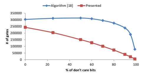
Figure 2: Results for random sequences of length $2^{20}$.

Design parameters						Bit-flipping	Presented	$\frac{G_{1}-G_{2}}{G_{1}}*100\%$
Name	# Gates	# Scan cells	# Faults	# Scan chains	# Top-off	# Gates, $G_{1}$	# Gates, $G_{2}$
a	34113	2511	91834	128	207	5049	4565	9.59
b	22104	1726	66390	128	214	4969	4515	9.14
c	19621	1726	48920	128	40	973	472	51.52
d	21984	1727	66554	128	211	5003	4470	10.65
e	19275	1727	50076	128	66	1224	684	44.11
f	39277	3022	89108	128	133	3820	3352	12.25
g	31726	2690	83936	128	213	5125	4674	8.80
h	29418	2690	67654	128	40	1191	577	51.55
average						3420	2880	24.7

TABLE II: Comparison to the bit-flipping approach for maximum achievable stuck-at faults coverage.

Design parameters		Maximum achievable stuck-at fault coverage				Stuck-at fault coverage $>98$%
Name	# Gates, $G_{1}$	# Top-off	% Test	Presented	$\frac{G_{1}-G_{2}}{G_{1}}*100\%$	# Top-off	% Test	Presented	$\frac{G_{1}-G_{3}}{G_{1}}*100\%$
			Coverage	# Gates, $G_{2}$			Coverage	# Gates, $G_{3}$
a	34113	207	99.98	4565	13.29	102	98.21	2004	5.87
b	22104	214	99.98	4515	20.28	63	98.30	1210	5.47
c	19621	40	99.98	472	2.24	40	99.98	427	2.17
d	21984	211	99.98	4470	20.18	67	99.13	1212	5.51
e	19275	66	99.98	684	3.38	66	99.98	647	3.36
f	39277	133	99.99	3352	8.45	100	99.46	2049	5.22
g	31726	213	99.98	4674	14.63	92	99.89	1771	5.58
h	29418	40	99.99	577	1.85	40	99.99	542	1.84

TABLE III: Area overhead of the presented approach for different stuck-at fault coverages.

V-B Comparison to previous approaches for embedding deterministic test patterns

In the second experiment, we compared the presented algorithms to the bit-flipping approach for embedding deterministic test patterns which, in our opinion, is one of the most efficient ones [12]. The results presented in this section were obtained using our implementation of the bit-flipping algorithm.

We applied both algorithms to 8 real designs with the number of gates varying from 19K to 39K. The results are summarized in Table II. We first applied 9000 pseudo-random patterns to all designs. Then, we computed the top-off patterns required to reach maximum achievable stuck-at faults coverage using a commercial ATPG tool. We used bit-flipping and the presented algorithms to represent these top-off patterns. As we can see from Table II, the presented approach outperforms the bit-flipping approach by 24.7% on average. The difference in the number of gates required in both approaches can be up to 51.5%. What is even more important, the area overhead of the presented approach goes down as the number of scan chains grows. On the contrary, the area overhead of the bit-flipping approach goes up (see Figure 3).

However, in spite of the improvements, the percentage of the overall chip area required to store deterministic test patterns can be prohibitively high for some designs (see column 6 of Table III). It is known that the size of representation for a data is related to the entropy of data [31]. Entropy puts a theoretical limit on the size of the minimal representation that can be achieved.

If a lower fault coverage is acceptable, then the area overhead can be reduced by exploiting the fact that don’t care bits are normally unevenly distributed among test patterns. As an example, consider the diagram in Figure 4. Each point on this diagram shows the number of don’t care bits in a test pattern of dma benchmark (in total 411 patterns of length 1720 bits each). These test patterns were generated by a commercial ATPG tool with dynamic compaction turned on and random fill turned off. They cover 100% of detectable stuck-at faults. The total percentage of specified bits is 6.45%. We can see that only the first few test patterns are highly specified. If we chop off the first 5% of test patterns, the entropy of the remaining patterns reduces twice. Therefore, they can be represented with a twice smaller representation than the one required for the whole set of test patterns. By using the last 95% of test patterns, we can achive 95.7% test coverage for stuck-at faults.

In Table III we show that, by using a subset of the top-off patterns only, we can reduce the area required for their representation more than 3 times in some cases, while sacrificing the fault coverage by less than 2%.

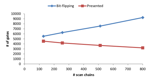
Figure 3: Area overhead as a function of the number of chains.

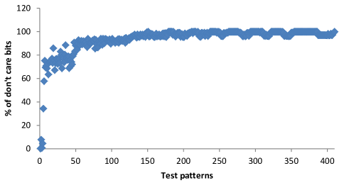
Figure 4: Distribution of don’t care bits in the test patterns of dma benchmark.

VI Conclusion

We presented a new method for embedding deterministic test patterns on-chip based on binary machines. The presented algorithm for synthesis of binary machines is significantly more efficient than previous work, especially for test data with many don’t cares. Our experimental results on 8 real designs show that the proposed approach outperforms the bit-flipping approach by 24.7% on average. We also show that it is possible to exploit uneven distribution of don’t care bits in test patterns to reduce the area required for generating top-off patterns more than 3 times with less than 2% decrease in fault coverage.

We believe that the presented algorithm for synthesis of binary machines is quite close to an optimal. What can be improved in the proposed method is the strategy for selecting a subset of top-off patterns which maximizes the fault coverage and minimizes the area overhead. At present, we use a simple greedy algorithm which selects top-off patterns based on the number of don’t care bits and the number of covered faults. A more sophisticated approach is likely to bring better results.

Binary machines can potentially be used for storing compressed test patterns for on-chip test compression techniques. This would eliminate the dependence of test compression on ATE memory. We are currently investigating the feasibility of such an approach on large industrial designs.

VII Acknowledgement

This work was supported in part by a research grant No 2011-03336 from the Swedish Governmental Agency for Innovation Systems VINNOVA.

References

- [1] Z. Wang and K. Chakrabarty, “Test data compression for IP embedded cores using selective encoding of scan slices,” in Proceedings of International Test Conference (ITC’2005), pp. 10 pp. –590, Nov. 2005.
- [2] “International technology roadmap for semiconductors,” 2011.
- [3] B. Koenemann, C. Barnhart, B. Keller, T. Snethen, O. Farnsworth, and D. Wheater, “A smartbist variant with guaranteed encoding,” in Proceedings of Asian Test Symposium (ATE’2001), pp. 325 –330, 2001.
- [4] J. Rajski, J. Tyszer, M. Kassab, and N. Mukherjee, “Embedded deterministic test,” IEEE Transactions on Computer-Aided Design of Integrated Circuits and Systems, vol. 23, pp. 776 – 792, May 2004.
- [5] S. Mitra and K. S. Kim, “X-compact: an efficient response compaction technique,” IEEE Transactions on Computer-Aided Design of Integrated Circuits and Systems, vol. 23, pp. 421 – 432, March 2004.
- [6] D. Czysz, G. Mrugalski, N. Mukherjee, J. Rajski, P. Szczerbicki, and J. Tyszer, “Deterministic clustering of incompatible test cubes for higher power-aware EDT compression,” IEEE Transactions on Computer-Aided Design of Integrated Circuits and Systems, vol. 30, pp. 1225 –1238, aug. 2011.
- [7] M. Majeed, D. Ahlstrom, U. Ingelsson, G. Carlsson, and E. Larsson, “Efficient embedding of deterministic test data,” in Proceedings of Asian Test Symposium (ATS’2010), pp. 159 –162, Dec. 2010.
- [8] D. Das and N. Touba, “Reducing test data volume using external/LBIST hybrid test patterns,” in Proceedings of International Test Conference (ITC’2000), pp. 115 –122, 2000.
- [9] E. B. Eichelberger and E. Lindbloom, “Random-pattern coverage enhancement and diagnosis for LSSD logic self-test,” IBM J. Res. Dev., vol. 27, pp. 265–272, May 1983.
- [10] C. Chin and E. J. McCluskey, “Weighted pattern generation for built-in self test,” Tech. Rep. TR - 84-7, Stanford Center for Reliable Computing, Aug. 1984.
- [11] G. Jervan, E. Orasson, H. Kruus, and R. Ubar, “Hybrid BIST optimization using reseeding and test set compaction,” Microprocess. Microsyst., vol. 32, pp. 254–262, August 2008.
- [12] H.-J. Wunderlich and G. Kiefer, “Bit-flipping BIST,” in Proc. of IEEE/ACM International Conference on Computer-Aided Design (ICCAD’1996), (San Jose, CA, USA), pp. 337 – 343, Nov. 1996.
- [13] J. Savir, G. S. Ditlow, and P. H. Bardell, “Random pattern testability,” IEEE Transactions on Computers, vol. C-33, pp. 79 –90, Jan. 1984.
- [14] G. Hetherington, T. Fryars, N. Tamarapalli, M. Kassab, A. Hassan, and J. Rajski, “Logic BISTfor large industrial designs: real issues and case studies,” in Proceedings of International Test Conference (ITC’1999), pp. 358 –367, 1999.
- [15] S. Golomb, Shift Register Sequences. Aegean Park Press, 1982.
- [16] C. J. Jansen, Investigations On Nonlinear Streamcipher Systems: Construction and Evaluation Methods. Ph.D. Thesis, Technical University of Delft, 1989.
- [17] E. Dubrova, “Synthesis of binary machines,” IEEE Transactions on Information Theory, vol. 57, pp. 6890 – 6893, 2011.
- [18] E. Dubrova, “Synthesis of parallel binary machines,” in Proceedings of International Conference of Computer-Aided Design (ICCAD’2011), (San Jose, CA, USA), pp. 200–206, Nov. 2011.
- [19] G. De Micheli, R. Brayton, and A. Sangiovanni-Vincentelli, “Optimal state assignment for finite state machines,” Computer-Aided Design of Integrated Circuits and Systems, IEEE Transactions on, vol. 4, pp. 269 – 285, July 1985.
- [20] T. W. Cusick and P. Stǎnicǎ, Cryptographic Boolean functions and applications. San Diego, CA, USA: Academic Press, 2009.
- [21] D. H. Green, “Families of Reed-Muller canonical forms,” International Journal of Electronics, vol. 70, pp. 259–280, 1991.
- [22] R. K. Brayton, C. McMullen, G. Hatchel, and A. Sangiovanni-Vincentelli, Logic Minimization Algorithms For VLSI Synthesis. Kluwer Academic Publishers, 1984.
- [23] T.-B. Pei and C. Zukowski, “High-speed parallel CRC circuits in VLSI,” Communications, IEEE Transactions on, vol. 40, pp. 653 –657, apr 1992.
- [24] S. Mukhopadhyay and P. Sarkar, “Application of LFSRs for parallel sequence generation in cryptologic algorithms,” in Computational Science and Its Applications - ICCSA 2006, vol. 3982 of Lecture Notes in Computer Science, pp. 436–445, Springer Berlin / Heidelberg, 2006.
- [25] C. D. Canniere and B. Preneel, “TRIVIUM specifications,” citeseer.ist.psu.edu/734144.html.
- [26] M. Hell, T. Johansson, and W. Meier, “Grain - a stream cipher for constrained environments,” citeseer.ist.psu.edu/732342.html.
- [27] I. Wegener, The Complexity of Boolean Functions. Stuttgart: John Wiley and Sons Ltd, 1987.
- [28] E. Dubrova, “A list of maximum-period NLFSRs,” March 2012. eprint.iacr.org/2012/166.
- [29] D. E. Knuth, The Art of Computer Programming Volumes 1-3 Boxed Set. Boston, MA, USA: Addison-Wesley Longman Publishing Co., Inc., 1998.
- [30] Berkeley Logic Synthesis and Verification Group, “ABC: A system for sequential synthesis and verification, release 70930,” 2007.
- [31] C. E. Shannon, “A mathematical theory of communications,” The Bell System Technical Journal, vol. 27, pp. 379–423,623–656, July,October 1948.