Abstract

This paper applies conformal prediction techniques to compute simultaneous prediction bands and clustering trees for functional data. These tools can be used to detect outliers and clusters. Both our prediction bands and clustering trees provide prediction sets for the underlying stochastic process with a guaranteed finite sample behavior, under no distributional assumptions. The prediction sets are also informative in that they correspond to the high density region of the underlying process. While ordinary conformal prediction has high computational cost for functional data, we use the inductive conformal predictor, together with several novel choices of conformity scores, to simplify the computation. Our methods are illustrated on some real data examples.

1 Introduction

Functional data analysis has been the focus of much research efforts in the statistics and machine learning community in the last decade. In functional data analysis, the data points are functions rather than scalars or vectors. The functional perspective provides a powerful modeling tool for many natural processes with certain smoothness structures. Typical examples arise in temporal-spatial statistics, longitudinal data, genetics, and engineering. The literature on functional data analysis is growing very quickly and familiar techniques like regression, classification, principal component analysis and clustering have all been extended to functional data. The books by Ramsay & Silverman (1997) and Ferraty & Vieu (2006) have established the state of the art.

The focus of this paper is exploratory analysis and visualization for functional data, including detection of outliers, median sets, and high density sets. Due to its infinite dimensional nature, visualization is a challenging problem for functional data since it is hard to see directly which curves are typical and which are abnormal. In the literature, many classical notions and tools for ordinary vector data have been extended to functional data, using either finite dimensional projection methods such as functional principal components (FPCA) and spline basis, or componentwise methods. For example, Hyndman & Shang (2010) developed functional bagplots and boxplots, where a band in functional space is obtained by first applying bivariate bagplots Rousseeuw et al. (1999) on the first two principal component scores, and projecting the bivariate sets back onto the functional space. In Sun & Genton (2011), the sample functions are ordered using a notion of functional data depth López-Pintado & Romo (2009) and a band is constructed by taking componentwise maximum and minimum of sample quantile functions. Other related work in outlier detection mostly use functional data depth to order the curves, and then apply robust estimators to detect outliers, see Cuevas et al. (2007), Febrero et al. (2008), Gervini (2009).

In this paper, we visualize functional quantiles in the form of simultaneous prediction bands. That is, for a given level of coverage, we construct a band that covers a random curve drawn from the underlying process. Our prediction bands are constructed by combining the finite dimensional projection approach and the idea of conformal prediction, a general approach to construct distribution free finite sample valid prediction sets Vovk et al. (2005); Shafer & Vovk (2008). Although originally developed as a tool for online prediction, conformal prediction methods have been proven to be useful for general nonparametric inferences, yielding robust and efficient prediction sets Lei et al. (2013); Lei & Wasserman (2013). To apply conformal methods to functional data, a major challenge is computation efficiency. Computing the bands with finite dimensional projection is infeasible using ordinary conformal prediction methods because the conformal prediction sets are usually hard to characterize. Here we use the inductive conformal method which allows efficient implementation for functional data when combined with some carefully chosen conformity scores. The resulting prediction bands always give correct finite sample coverage, without any regularity conditions on the underlying process. Unlike many existing functional boxplots, our bands tend to reflect the “high density” regions in the functional spaces and may have disconnected slices. In some cases, such a property can also reveal other salient structures in the data such as clusters.

Another contribution of this paper is the construction of clustering trees with finite sample interpretation for functional data. In classical vector cases, clustering, together with the aforementioned prediction sets, is closely related to density level sets Hartigan (1975); Rinaldo & Wasserman (2010); Rinaldo et al. (2012). However, in functional spaces, the density is not well defined because there is no $\sigma$-finite dominating measure. In Ferraty & Vieu (2006), a notion of “pseudo density” is used instead of density. In context of functional data, most methods use finite dimensional projections, combined with classical clustering methods such as K-means Tarpey & Kinateder (2003); Antoniadis et al. (2010) and Gaussian mixtures James & Sugar (2003); Shi & Wang (2008). A componentwise approach to functional data clustering is studied by Delaigle et al. (2012). In this paper we construct clustering trees for functional data by combining the pseudo density idea Ferraty & Vieu (2006) and conformal prediction. Each level of our cluster tree corresponds to an estimated prediction set, with distribution free, finite sample coverage. The clustering trees are therefore naturally indexed by the level of coverage. Moreover, the prediction sets at a higher level on the tree correspond to regions with higher pseudo density.

To our knowledge, this paper is the first to do prediction and visualization of functional data with finite sample guarantees. In Section 2 we introduce the problem of prediction bands for functional data and the general idea of conformal prediction method under this context. In Section 3 we develop the extended conformal prediction and apply it to efficiently construct simultaneous prediction bands for function data with good finite sample property. In Section 4 we develop our method of conformal cluster tree. Both methods are illustrated through real data examples.

2 Notation and Background

2.1 Prediction Sets for Functional Data

Let $X_{1}(\cdot),\cdots,X_{n}(\cdot)$ denote $n$ random functions drawn from an unknown distribution $P$ over the set of functions on $[0,1]$ with finite energy: ${\Omega}=L_{2}[0,1]$. The distribution $P$ is defined on an appropriate $\sigma$-field ${\cal F}$ on ${\Omega}$. Given the data and a number $0<\alpha<1$, we will construct a set of functions ${\cal C}_{n}\subset{\Omega}$ such that, for all $P$ and all $n$,

$$\mathbb{P}(X_{n+1}\in{\cal C}_{n})\geq 1-\alpha$$ (1)

where $X_{n+1}$ denotes a future function drawn from $P$ and $\mathbb{P}$ denotes the probability corresponding to $P^{n+1}$, the product measure induced by $P$.

Requiring (1) to hold is very ambitious and may be more than needed. If we are only interested in the main structural features of the curve, then we instead aim for the more modest goal that, for all $P$ and all $n$,

$$\mathbb{P}(\Pi(X_{n+1})\in{\cal C}_{n})\geq 1-\alpha$$ (2)

where $\Pi$ is a mapping into a finite dimensional function space ${\Omega}_{p}\subset{\Omega}$. The projection $\Pi$ may correspond to the subspace spanned by the first few functions in Fourier basis, wavelet basis, or any other orthonormal basis of $L_{2}[0,1]$.

In practice it is often of interest (for example, for visualization purposes) to have prediction bands. A prediction band $\mathcal{B}_{n}$ is a prediction set of the form $\mathcal{B}_{n}=\{X(\cdot)\in L_{2}[0,1]:X(t)\in B_{n}(t),\leavevmode\nobreak\ \forall\leavevmode\nobreak\ t\in[0,1]\}$, where for each $t$, $B_{n}(t)\subseteq{}^{1}$ can be expressed as the union of finitely many intervals. Most existing prediction bands for functional data with provable coverage relies on the assumption of Gaussianity (see, for example, Yao et al. (2005)). It is desirable to construct distribution free, finite sample prediction bands for functional data under general distributions.

2.2 Conformal Prediction Methods and Variants

Conformal inference Vovk et al. (2005); Shafer & Vovk (2008) is a very general theory of prediction, focused on sequential prediction. For our purposes, we only need the following batch version. Given the observed objects (random variables, random vectors, random functions, etc.) $X_{1},\ldots,X_{n}$ we want a prediction set for a new object $X_{n+1}$. Assume that $X_{i}\in{\Omega}$ and let $x\in{\Omega}$ be a fixed, arbitrary object. We will test the null hypothesis that $X_{n+1}=x$ and then take ${\cal C}_{n}$ to be the set of $x$’s that are not rejected by the test. Here are the details.

Define the augmented data ${\sf aug}(x)=\{X_{1},\ldots,X_{n},x\}$. Define conformity scores $\sigma_{1},\ldots,\sigma_{n+1}$ where $\sigma_{i}=g(X_{i},{\sf aug}(x))$ for some function $g$. (Actually, in Vovk et al. (2005) they omit $X_{i}$ from $g$ when defining $\sigma_{i}$. We discuss this point at the end of this section.) For $i=n+1$, the score is defined to be $\sigma_{n+1}=g(x,{\sf aug}(x))$. The conformity score measures how similar $X_{i}$ is to the rest of the data. An example is $\sigma_{i}=-\int(X_{i}(t)-\overline{X}^{x}(t))^{2}dt$ where

$\overline{X}^{x}(t)=(n+1)^{-1}[x(t)+\sum_{i=1}^{n}X_{i}(t)].$

In fact, we will use some other conformity scores that are better adapted to the data distribution.

Consider testing the null hypothesis $H_{0}:X_{n+1}=x$. When $H_{0}$ is true, the objects in the set ${\sf aug}(x)=\{X_{1},\ldots,X_{n},x\}$ are exchangeable and so the ranks of the conformity scores are uniformly distributed. Thus, the p-value

$$\pi(x)=\frac{\sum_{i=1}^{n+1}1{\hskip-2.5pt}\hbox{I}(\sigma_{i}\leq\sigma_{n+1})}{n+1}$$ (3)

is uniformly distributed over $\{1/(n+1),2/(n+1),...,1\}$ and is a valid p-value for the test in the sense that $\mathbb{P}[\pi_{n}(X_{n+1})\geq\alpha]\geq 1-\alpha$. We now invert the test, that is, we collect all the non-rejected null hypotheses:

$${\cal C}_{n}=\{x:\ \pi(x)\geq\alpha\}.$$ (4)

It follows from the above argument that

$$\mathbb{P}(X_{n+1}\in{\cal C}_{n})\geq 1-\alpha$$ (5)

for any $P$ and $n$. We refer to the above construction as the standard conformal method. Next we discuss the use of inductive conformal method which, as we shall see, has some computational advantages. The general idea is first given in Section 4.1 of Vovk et al. (2005).

Algorithm 1: Inductive Conformal Predictor Input: Data $X_{1},...,X_{n}$, confidence level $1-\alpha$, $n_{1}<n$. Output: ${\cal C}_{n}$. 1. Split data randomly into two parts $\mathbf{X}_{1}=\{X_{1},...X_{n_{1}}\}$, and $\mathbf{X}_{2}=\{X_{n_{1}+1},...,X_{n}\}$. Let $n_{2}=n-n_{1}$. 2. Let $g:\Omega\mapsto\mathbb{R}$ be a function constructed from $X_{1},\ldots,X_{n_{1}}$. 3. Define $\sigma_{i}=g(X_{n_{1}+i})$ for $i=1,\ldots,n_{2}$. Let $\sigma_{(1)}\leq\cdots\leq\sigma_{(n_{2})}$ denote the ranked values. 4. Let ${\cal C}_{n}=\{x:\ g(x)\geq\lambda\}$ with $\lambda=\sigma_{(\lceil(n_{2}+1)\alpha\rceil-1)}$.

Lemma 2.1.

Let $\mathcal{C}_{n}$ be the output of Algorithm 1. For all $n$ and $P$, $\mathbb{P}(X_{n+1}\in{\cal C}_{n})\geq 1-\alpha$.

Proof.

Note that the random function $g(\cdot)$ is independent of $\mathbf{X}_{2}$. Assume $X_{n+1}$ is another random sample. By exchangeability, the rank of $\sigma_{n_{2}+1}:=g(X_{n+1})$ among $\{\sigma_{1},...,\sigma_{n_{2}+1}\}$ is uniform among $\{1,2,...,n_{2}+1\}$. Therefore with probability at least $1-\alpha$, $X_{n+1}$ falls in $\mathcal{C}_{n}$. ∎

In the rest of this paper, unless otherwise noted, we use $n_{1}=\lfloor n/2\rfloor$. The data splitting step might seem inefficient due to the sample splitting. However, it greatly reduces the computational burden of the standard conformal method by avoiding re-fitting the function $g$ with every augmented data ${\sf aug}(x)$ for all $x\in\Omega$. Moreover, such a reduction can also substantially improve the robustness of the resulting prediction sets. For example, consider $k$-means clustering in $d$-dimensional Euclidean space. Let $\mathbf{Z}=(Z_{1},...,Z_{n})\subset{}^{d}$ be a data set. Given $k$ centers $v_{1},\ldots,v_{k}\subset{}^{d}$, let

$$R(v_{1},...,v_{k})=\frac{1}{n}\sum_{i=1}^{n}\min_{j}\|v_{j}-Z_{i}\|_{2}^{2}.$$

The $k$-means prototypes are the functions $\widehat{v}_{1},\ldots,\widehat{v}_{k}$ that minimize $R$. As usual, we can partition the data into $k$ groups $\widehat{G}_{1},\ldots,\widehat{G}_{k}$ where $\widehat{G}_{j}=\{Z_{i}:\|Z_{i}-\widehat{v}_{j}\|\leq\|Z_{i}-\widehat{v}_{r}\|,r\neq j\}$.

For the standard conformal method, let $\widehat{v}_{1}(z),\ldots,\widehat{v}_{k}(z)$ denote the prototypes based on the augmented data $Z_{1},\ldots,Z_{n},z$. Define the conformity score $\sigma_{i}=-\min_{j}\|Z_{i}-\widehat{v}_{j}(z)\|$. Let ${\cal C}_{n}$ denote the resulting conformal set. With obvious modification, let ${\cal C}_{n}^{\prime}$ denote the conformal set based on the modified method. Define ${\sf diam}(\mathcal{C})=\sup_{x,y\in\mathcal{C}}\|x-y\|$.

Proposition 2.1.

For any $\mathbf{Z}$, ${\sf diam}({\cal C}_{n})=\infty$ but ${\sf diam}({\cal C}_{n}^{\prime})<\infty$ if $n>2/\alpha$.

Proof.

For the first statement, consider the augmented data $Z_{1},\ldots,Z_{n},z$, where $\|z\|\geq C$. For $C$ sufficiently large (may depend on $\mathbf{Z}$), there exists a group $G_{j}$ such that $G_{j}=\{z\}$. In this case, $\sigma_{n+1}=0$ and hence ${\cal C}_{n}\supseteq\{z:\|z\|\geq C\}$ for all $\alpha$. It follows that ${\sf diam}({\cal C}_{n})=\infty$. The second statement follows since all the prototypes are in ${\sf convhull}(\mathbf{Z}_{1})\subseteq{\sf convhull}(\mathbf{Z})$. For all $\alpha$, there exists a $C>0$ large enough such that $g(z)<\sigma_{1}$ for all $\|z\|\geq C$. The key is that in the modified method, the prototypes and the majority of $\sigma_{i}$’s are not affected by absurd values of $z$. ∎

Remark 2.1.

Bounded prediction sets could also be obtained by omitting $Y_{i}$ from $g$ when defining $\sigma_{i}$. This is, in fact, the method used in Vovk et al. (2005). But this “omit one” approach is much more computationally expensive than our data-splitting method.

2.3 Conformal Prediction Bands in the Functional Case

We conclude this section with a brief discussion on conformal prediction bands for functional data. When the $X_{i}$’s are functions, we can construct prediction bands as follows. Given ${\cal C}_{n}$, a conformal prediction set, we can define upper and lower bounds for all $t\in[0,1]$: $\ell(t)=\inf_{x\in{\cal C}_{n}}x(t)$ and $u(t)=\sup_{x\in{\cal C}_{n}}x(t).$ It follows that

$$\mathbb{P}[\ell(t)\leq X_{n+1}(t)\leq u(t),\leavevmode\nobreak\ \forall\leavevmode\nobreak\ t]\geq 1-\alpha.$$

However, these bounds may be hard to compute, depending on the choice of conformity score.

The choice of conformity score also affects statistical efficiency. To see this, consider the following example. Under mild conditions on the process, the random variable $Y=\sup_{t}|X(t)|$ has finite quantiles. Then we can construct conformal prediction set $\mathcal{C}_{n}$ using the standard approach with conformity score $g(X)=-\sup_{t}|X(t)|$. Thus $\mathcal{C}_{n}$ is a valid prediction set and naturally leads to a band. However, such a band is usually too wide and hence of limited use.

We therefore face two challenges: choosing a good conformity score and extracting useful information from ${\cal C}_{n}$. In the vector setting, Lei et al. (2013) showed that using a density estimator to define a conformity score leads to conformal set ${\cal C}_{n}$ with certain minimax optimality properties. However, in the present setting, densities do not even exist. Instead, we consider two approaches: the first uses density of coefficients of projections to construct prediction bands and the second uses pseudo-densities to build clustering trees.

There is also a third challenge: identifying an optimal conformity score. This was done using minimax theory in Lei et al. (2013); Lei & Wasserman (2013) in the case where the data are vectors. To our knowledge, choosing an optimal conformity score for the functional case is still an open question. Rather, our current focus is on computation and visualization.

3 Prediction Bands Based on Projections

A common approach to functional data analysis is to project the curves onto a finite dimensional space that captures the main features of the curves. In this section, we consider the projection approach because it enables us to characterize the prediction sets and to construct simultaneous prediction bands with finite sample guarantee. To be concrete, we require the prediction band ${\cal C}_{n}$ to satisfy $\mathbb{P}(\Pi(X_{n+1})\in{\cal C}_{n})\geq 1-\alpha$ where $\Pi$ is a mapping into a $p$-dimensional function space ${\Omega}_{p}\subset{\Omega}$. There are two types of projections: projections on a fixed basis (for example, Fourier basis, wavelet basis, and spline basis) and projections on a data-driven basis such as functional principal components (FPC). Our method, summarized in Algorithm 2, is general enough so that it can be used for any basis. It is a specific implementation of the general method given in Algorithm 1.

Algorithm 2: Functional Conformal Prediction Bands Input: Data $X_{1},...,X_{n}$, basis functions $(\phi_{1},...\phi_{p})$, conformity score $\widehat{f}$, level $\alpha$, $1\leq n_{1}<n$. Output: $B_{n}(t)\subseteq{}^{1}$ for all $t\in[0,1]$. 1. Split data randomly into two parts $\mathbf{X}_{1}=\{X_{1},...X_{n_{1}}\}$, and $\mathbf{X}_{2}=\{X_{n_{1}+1},...,X_{n}\}$. Let $n_{2}=n-n_{1}$. 2. Compute basis projection coefficients $\xi_{ij}=\langle X_{i},\phi_{j}\rangle$, for $i=1,...,n$, $j=1,...,p$. Denote $\xi_{i}=(\xi_{i1},...,\xi_{ip})$. 3. For $i=n_{1}+1,...,n$, evaluate $\widehat{f}(\xi_{i})=\widehat{f}(\xi_{i};\xi_{1},...,\xi_{n_{1}})$ and rank these numbers by $f_{1}\leq f_{2}\leq...\leq f_{n_{2}}$. 4. Define $T_{n}=\{\xi\in{}^{p}:\widehat{f}(\xi)\geq\lambda=f_{\lceil(n_{2}+1)\alpha\rceil-1}\}$. 5. $B_{n}(t)=\{\sum_{j=1}^{p}\zeta_{j}\phi_{j}(t):(\zeta_{1},...,\zeta_{p})\in T_{n}\}$.

Proposition 3.1.

Denote $\Pi_{p}$ the projection operator induced by eigen-functions $\{\phi_{j}:1\leq j\leq p\}$. Then the prediction band $\mathcal{B}_{n}$ given by Algorithm 2 satisfies

$$\mathbb{P}\big{\{}\left(\Pi_{p}X_{n+1}\right)(t)\in B_{n}(t),\leavevmode\nobreak\ \forall\leavevmode\nobreak\ t\in[0,1]\big{\}}\geq 1-\alpha.$$

The proof follows from that of Lemma 2.1.

Remark 3.1.

The above finite sample coverage guarantee remains valid if the basis functions are estimated from $\mathbf{X}_{1}$, which is the case in most applications where functional principal components are used.

3.1 Conformal Prediction Bands using Gaussian Mixture Approximation

In general one can apply Algorithm 2 with any basis (possibly a data-driven one obtained from $\mathbf{X}_{1}$). However, in its abstract form, Algorithm 2 leaves some implementation issues unsolved. The most challenging one is the characterization of $T_{n}$ and $B_{n}(t)$ which depend on the choice of conformity score. Usually $\widehat{f}$ is a density estimator of the projection coefficient vector $\xi\in{}^{p}$ since it makes sense to use high density region as a prediction set for future observations. For example, Lei et al. (2013) use kernel density estimator to construct $\widehat{f}$. Although kernel density estimators can approximate any smooth densities, it is unclear how to keep track of $\{\xi^{T}\phi(t):\xi\in T_{n}\}$, the linear projection of the resulting prediction sets, where $\phi(t)=(\phi_{1}(t),...,\phi_{p}(t))^{T}$. However, the inductive conformal method allows us to use any other conformity score to simplify the computation. Next we show how to use Gaussian mixture density estimator to construct such a band.

To motivate the method, consider the mixture model

$$X\sim P=\pi_{1}P_{1}+\pi_{2}P_{2}+\cdots+\pi_{K}P_{K},$$

where each $P_{k}$ is the distribution of a Gaussian process on $[0,1]$ and $\pi_{k}$’s are mixing probabilities satisfying $\sum_{k}\pi_{k}=1$ and $\pi_{k}\geq 0$. Let $\{\phi_{j}:j\geq 1\}$ be an orthonormal basis of $L_{2}[0,1]$, and $\xi_{j}=\langle X,\phi_{j}\rangle$ be the scores of $X$, where $\langle f,g\rangle=\int fg$. Then $(\xi_{1},...,\xi_{p})$ is distributed as a $p$-dimensional Gaussian mixture. For smooth processes, the variance of the projection score on dimension $j$ in each component decays quickly as $j$ grows. Therefore, it is common in functional data analysis the sequence of scores is truncated for some small $p$. The basis that gives fastest decay corresponds to the functional principal components, where $\phi_{j}$’s are the eigen-functions of $\Gamma$, the covariance function of $X$:

$\Gamma=\mathbb{E}[X\otimes X]-\mathbb{E}X\otimes\mathbb{E}X=\sum_{j\geq 1}\lambda_{j}\,[\phi_{j}\otimes\phi_{j}],$

where for functions $f,g\in L_{2}[0,1]$, we define $f\otimes g:[0,1]^{2}\mapsto\mathbb{R}^{1}$: $[f\otimes g](s,t)=f(s)g(t).$ We emphasize that our band has correct coverage: (1) without assuming that the mixture model is correct, and (2) for all choices of projection dimension and numbers of mixture components.

Going back to Algorithm 2, we can choose $\widehat{f}$ to be a Gaussian mixture density estimator with $K$ components and $\phi_{1},...,\phi_{p}$ the first $p$ eigen-functions of empirical covariance function obtained from $\mathbf{X}_{1}$. Let $\widehat{\pi}_{k},\leavevmode\nobreak\ \widehat{\mu}_{k},\leavevmode\nobreak\ \widehat{\Sigma}_{k}$ be the estimated mixture proportion, mean, and covariance of the $k$th component. Denote $\varphi(\cdot;\mu,\Sigma)$ the density function of ${\rm Norm}(\mu,\Sigma)$. A rough outer bound of $T_{n}$, the level set of $\widehat{f}$ at $\lambda$, can be obtained by

$$T_{n}=\{\xi:\widehat{f}(\xi)\geq\lambda\}\subseteq\bigcup_{k=1}^{K}\{\xi:\varphi(\xi;\widehat{\mu}_{k},\widehat{\Sigma}_{k})\geq\lambda/(K\widehat{\pi}_{k})\}:=\bigcup_{k=1}^{K}T_{n,k}.$$ (6)

Note that each $T_{n,k}$ is an ellipsoid in $\mathbb{R}^{p}$ whose projection on $\phi(t)$ can be computed easily. Let $u_{k}(t)=\sup_{\xi\in T_{n,k}}\xi^{T}\phi(t)$ and $\ell_{k}(t)=\inf_{\xi\in T_{n,k}}\xi^{T}\phi(t)$. Both $u_{k}$ and $\ell_{k}$ are available in close form. Then we can output $B_{n}(t)=\cup_{k}[\ell_{k}(t),u_{k}(t)]$.

3.2 Two refinements

The approximation in (6) is usually conservative and improvements are usually possible. We elaborate this idea in two cases.

A better approximation of the density level set.

First, when the components in the Gaussian mixture are well separated ($\widehat{\mu}_{k}$’s are far from each other), then intuitively the level set of $\widehat{f}$ at $\lambda$ shall be approximately the union of level sets of $\varphi(\cdot;\widehat{\mu}_{k},\widehat{\Sigma}_{k})$ at $\lambda/\pi_{k}$. Now we make this idea precise and give an more refined approximation of $T_{n}$ that also retains finite sample coverage guarantee.

For all $1\leq k,s\leq K$, define

$$\delta_{ks}=\sup_{\xi}\left(\widehat{\pi}_{k}\varphi(\xi;\widehat{\mu}_{k},\widehat{\Sigma}_{k})\wedge\widehat{\pi}_{s}\varphi(\xi;\widehat{\mu}_{s},\widehat{\Sigma}_{s})\right),\ \ \ \delta_{k}=\sum_{s\neq k}\delta_{ks}.$$

Roughly speaking, $\delta_{ks}$ measures how much the two components overlap and $\delta_{k}$ measures how much the $k$th component overlaps with all other components. We note that $\delta_{ks}$ can be computed by solving a sequence of simple quadratically constrained quadratic programming (QCQP). More concretely, for a given value of $c$, we find $\sup_{\xi}\varphi(\xi;\widehat{\mu}_{k},\widehat{\Sigma}_{k})$ under the constraint $\varphi(\xi;\widehat{\mu}_{s},\widehat{\Sigma}_{s})\geq c$, which is a simple QCQP. Denote this value by $\eta(c)$, then it can be shown that $\delta_{ks}$ is either trivial ($\widehat{\pi}_{s}\varphi(\mu;\widehat{\mu}_{s},\widehat{\Sigma}_{s})\leq\widehat{\pi}_{k}\varphi(\mu;\widehat{\mu}_{k},\widehat{\Sigma}_{k})$) or it can be given by the unique $c^{*}$ such that $\widehat{\pi}_{k}c^{*}=\widehat{\pi}_{s}\eta(c^{*})$. In the non-trivial case, $c^{*}$ can be found using a simple binary search.

When all $\delta_{k}$ are smaller than $\lambda$, we have a better approximation of $T_{n}$:

$$T_{n}=\{\xi:\widehat{f}(\xi)\geq\lambda\}\subseteq\bigcup_{k=1}^{K}\{\xi:\varphi(\xi;\widehat{\mu}_{k},\widehat{\Sigma}_{k})\geq(\lambda-\delta_{k})/\pi_{k}\}:=\bigcup_{k=1}^{K}\tilde{T}_{n,k}.$$ (7)

Note that $\tilde{T}_{n,k}$ is also an ellipsoid. We can similarly compute $\tilde{\ell}_{k}=\inf_{\xi\in\tilde{T}_{n,k}}\xi^{T}\phi(t)$, $\tilde{u}_{k}=\sup_{\xi\in\tilde{T}_{n,k}}\xi^{T}\phi(t)$, and the band $\tilde{B}_{n}(t)=\cup_{k}[\tilde{\ell}_{k},\tilde{u}_{k}]$.

Proposition 3.2.

The prediction band $\tilde{B}_{n}(t)$ constructed above is a union of $K$ bands, and

$$\mathbb{P}\left\{\exists\,k:\,\left[\Pi_{p}(X_{n+1})\right](t)\in[\tilde{\ell}_{k}(t),\tilde{u}_{k}(t)],\,\forall\,t\right\}\geq 1-\alpha.$$

We implement this method on a real data example. The data set consists of 1,000 recordings of neurons over time (see Figure 1 (a)). The data come from a behavioral experiment, performed at the Andrew Schwartz motorlab: A macaque monkey performs a center-out and out-center target reaching task with 26 targets in a virtual 3D environment. The curves show voltage of neurons versus times recorded at electrodes. The recorded neural activity consists of all action potentials detected above a channel-specific threshold on a 96-channel Utah array implanted in the primary motor cortex. One of the goals is “spike sorting” which means clustering the curves. Each cluster is thought to correspond to one neuron since each neuron tends to have a characteristic curve (spike).

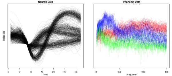
Figure 1: Two functional data sets. (a): neuron data. (b): phoneme data.

Our implementation uses functional principal components with $p=2$ and $K=3$. A band consists of three components is plotted along with the projected sample curves. The empirical coverage is 916 out of 1000. See Figure 2.

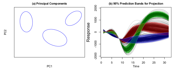
Figure 2: Prediction Bands for Neuron Data. (a): plots of first two FPC coefficients with boundary of $\tilde{T}_{n,k}$. (b): conformal prediction bands and projected curves.

A different conformity score.

The approximation introduced above may still be too conservative when the mixture components are not well separated. An example of such a situation can be seen from the phoneme data, which is considered in Hastie et al. (2009) and Ferraty & Vieu (2006). The data considered here consists of three phonemes, where each phoneme has 400 sample curves of discretized periodograms of length 150. The data is plotted in Figure 1 (b).

When analyzing the phoneme data, we also perform a FPCA and focus on the first two principal component scores. Note that our method can be implemented using other variants such as robust FPCA and using more dimensions. Here we choose two principal components for the ease of visualization. In the original data, the label of each curve is known and we summarize this information in Figure 3 (a) (but our algorithm assumes that the labels are unknown). We observe that the cluster corresponding to phoneme “dcl” exhibits significant non-Gaussianity, therefore the Gaussian mixture model fitting suggests that this single cluster is best modeled by a two-component Gaussian mixture. The band for that cluster is just the union of the bands given by the two components.

In this case, if the approximation in (7) is used, the resulting prediction and hence the band will be too wide than necessary due to the heavy overlap between the two components corresponding to phoneme “dcl”. Here we use a different conformity score to obtain a better prediction set. In particular, consider

$$\widehat{f}(\xi)=\max_{k:1\leq k\leq K}\widehat{\pi}_{k}\varphi(\xi;\widehat{\mu}_{k},\widehat{\Sigma}_{k}).$$ (8)

That is, instead of computing the sum of density from each component, we only look at the density of the cluster that $\xi$ is most likely to belong to. Such a conformity score function resembles that of a K-means clustering, except it takes into account of the mixture probabilities.

The advantage of using such a max function is the decomposability:

$$T_{n}=\{\xi:\widehat{f}(\xi)\geq\lambda\}=\bigcup_{k=1}^{K}\{\xi:\varphi(\xi;\widehat{\mu}_{k},\widehat{\Sigma_{k}})\geq\lambda/\widehat{\pi}_{k}\}:=\bigcup_{k=1}^{K}\bar{T}_{n,k}.$$ (9)

Since $\bar{T}_{n,k}$ is also an ellipsoid, we can analogously define $\bar{\ell}_{k}(t)=\inf_{\xi\in\bar{T}_{n,k}}\xi\phi(t)$, $\bar{u}_{k}(t)=\sup_{\xi\in\bar{T}_{n,k}}\xi^{T}\phi(t)$, and $\bar{B}_{n}(t)=\cup_{k}[\bar{\ell}_{k}(t),\bar{u}_{k}(t)]$.

Remark 3.2.

We note that $\bar{T}_{n,k}$ defined in (9) and $\tilde{T}_{n,k}$ defined in (7) are very close if the components are well-separated because $\delta_{k}\approx 0$ for all $k$ and $\widehat{f}$ defined in (8) is very close to the estimated density.

Since the union representation in the above equation is exact, there is no loss of statistical efficiency. The only possible loss of efficiency is using a conformity score function other than the density function. However, such a loss is conceivably small: since if the max contributor is large, the density is likely to be large. Therefore, ranking the max component density is roughly the same as ranking the density. The prediction band for the phoneme data is plotted in Figure 3 (b) where the empirical coverage is 90.5%.

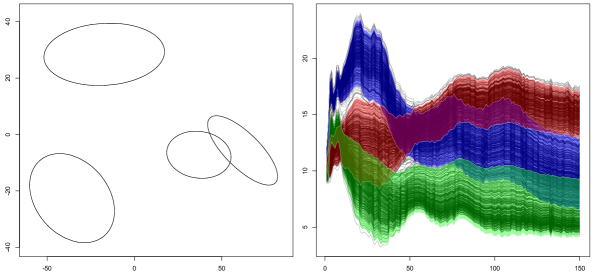
Figure 3: Prediction Bands for Phoneme Data. (a): plots of first two FPC coefficients with boundary of $\tilde{T}_{n,k}$. (b): conformal prediction bands and projected curves.

4 Methods Based on Pseudo-Densities

Here we investigate a different approach, based on pseudo-densities which were introduced by Ferraty & Vieu (2006). For simplicity, assume $n\alpha$ is an integer. Given a kernel $K$ and bandwidth $h>0$ define the pseudo-density estimator

$$\widehat{p}_{h}(u)=\frac{1}{n}\sum_{i=1}^{n}K\left(\frac{d(u,X_{i})}{h}\right)$$ (10)

where $d(f,g)$ is some distance measure (for example, $d(f,g)=[\int(f-g)^{2}]^{1/2}$). We assume that $K(z)\leq K(0)$ for all $z$. This looks like a kernel density estimator but it is not a density function. Indeed, there are no density functions on ${\Omega}$ because there is no $\sigma$-finite dominating measure. Nevertheless, Ferraty and Vieu show that $\widehat{p}_{h}(u)$ can be used for various tasks such as clustering curves, just as we would do for a density estimator. We can view $\widehat{p}_{h}$ as an estimator of $p_{h}(u)=\mathbb{E}(\widehat{p}_{h}(u))=\int K\big{(}\frac{d(u,x)}{h}\big{)}dP(x).$

We follow a similar approach here, and endow the high density sets in the functional space with a conformal prediction interpretation. For presentation simplicity, we use the standard conformal method. Let ${\cal C}_{n,\alpha}=\{f:\ \pi(f)\geq\alpha\}$ where

$$\pi(f)= \frac{1+\sum_{i=1}^{n}1{\hskip-2.5pt}\hbox{I}(\widehat{p}_{h}^{f}(X_{i})\leq\widehat{p}_{h}^{f}(f))}{n+1},$$

$$\widehat{p}_{h}^{f}(u)= \frac{n}{n+1}\widehat{p}_{h}(u)+\frac{1}{n+1}K\left(\frac{d(u,f)}{h}\right).$$

It is straightforward to see that $\mathcal{C}_{n,\alpha}$ constructed above is a level $1-\alpha$ conformal prediction set, and hence has distribution-free, finite sample coverage. The set ${\cal C}_{n,\alpha}$ can be approximated by a level set of $\widehat{p}_{h}$ as follows. Let $X_{(1)},X_{(2)},\ldots,$ denote the re-ordered data, ranked so that $\widehat{p}_{h}(X_{(1)})\leq\widehat{p}_{h}(X_{(2)})\leq\cdots$. Let $\lambda=\widehat{p}_{h}(X_{(n\alpha)})$ and let

$${\cal C}_{n,\alpha}^{+}=\left\{f:\ \widehat{p}_{h}(f)\geq\lambda-n^{-1}K(0)\right\}.$$ (11)

We have the following result ensuring that the level sets of the pseudo-density have a well-defined finite sample predictive interpretation. Its proof is analogous to that of ordinary kernel density for vectors (see Lei et al. (2013)).

Lemma 4.1.

We have $\mathbb{P}(X_{n+1}\in{\cal C}_{n,\alpha})\geq 1-\alpha$ for all $P$ and $n$. Furthermore, ${\cal C}_{n,\alpha}\subseteq{\cal C}_{n,\alpha}^{+}$ and hence, $\mathbb{P}(X_{n+1}\in{\cal C}_{n,\alpha}^{+})\geq 1-\alpha$ for all $P$ and $n$.

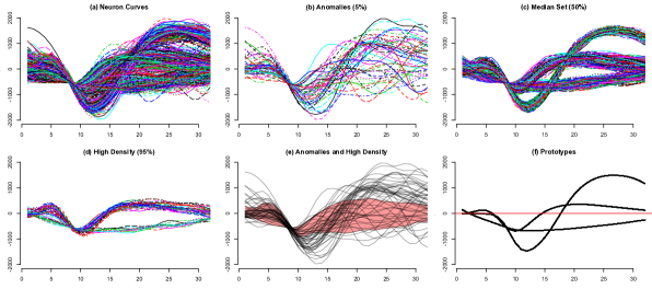
Figure 4: Neuron data. $X$ axis: time. $Y$ axis: response. (a) 1,000 recordings of action potentials over time. (b-e) anormalies, median, and high density sample curves using pseudo-density. (f) mean-shift prototypes.

Now we describe how to make use of and explore the set ${\cal C}_{n,\alpha}^{+}$. Let $\widehat{\mathcal{C}}_{n,\alpha}={\cal C}_{n,\alpha}^{+}\cap\{X_{1},\ldots,X_{n}\}$.

Anomalies, median set, and high density curves

We first consider three such sets of $\widehat{\cal C}_{n,\alpha}$: anomalies ($\alpha$ close to 0), typical ($\alpha=.5$) and high density ($\alpha$ close to 1). Figures 4 (b-e) show the results using the distance $d^{2}(f,g)=\int(f(t)-g(t))^{2}dt$ for the neuron data. It is easily seen that the median set successfully captures the common shape of each group of neurons. The high density set contains curves in the two larger groups. The anomalies consist of mostly curves with irregular shape.

Modes, prototypes, and mean shift

Another summary of $\widehat{\cal C}_{n,\alpha}$ are prototypes, that is, representative functions corresponding to the local maxima of the pseudo density (see also the cluster tree below). The modes of the pseudo-density can be obtained using the mean-shift algorithm Cheng (1995). Figure 4 (f) shows the three modes obtained in our example. Two of the modes have the signature of a neuron firing (a decrease followed by a sharp increase). The third mode, which stays negative, is unusual and deserves further attention.

Conformal cluster tree

Here we use a cluster tree to visualize how the conformal prediction set evolves as $\alpha$ changes smoothly from $0$ to $1$. For a given $\epsilon>0$, define the graph $G_{\alpha,\epsilon}$ whose nodes correspond to the functions in $\widehat{\cal C}_{n,\alpha}$ and with edges between nodes $X_{i}$ and $X_{j}$ if $\int(X_{i}(t)-X_{j}(t))^{2}dt\leq\epsilon^{2}$. Define the level $\alpha$ clusters to be the partition of $\widehat{\cal C}_{n,\alpha}$ induced by connected components of $G_{\alpha,\epsilon}$. As the conformal parameter $\alpha$ varies from $0$ to $1$, the collection $\mathcal{T}$ of all level $\alpha$ clusters form a tree (i.e. $A,B\in\mathcal{T}$ implies that $A\cap B=\emptyset$ or $A\subset B$ or $B\subset A$), which we call the conformal tree. The height of the tree is indexed by $\alpha$, with the root of tree indexed by $\alpha=0$, corresponding to all the points in the dataset. As $\alpha$ increases the sets $\widehat{\cal C}_{n,\alpha}$ becomes smaller, and the leaves, which are associated to local modes of the pseudo density, consist each of a single data point. Such a conformal tree is similar to an ordinary clustering tree, plus the additional feature of finite sample coverage and a different but quite natural indexing on $\alpha$ rather than the usual indexing on the density itself.

The conformal tree provides a graphical representation of some distributional properties of the data and, in particular, of the “high-density” regions. As such it allows us to identify salient features about the data that may be otherwise hard to detect. Figure 5(a) shows the conformity tree of the neuron data based on the pseudo density estimator described above using the $L_{2}$ distance and the Gaussian kernel. It is easy to see how the data appear to arise from a mixture of three components (compare with Figure 2), with splits occurring at values of $\alpha$ equal to approximately $0.08$ and $0.24$. A further, more subtle, split occurs at $\alpha=0.79$, and distinguishes between two groups of curves exhibiting very similar but ultimately distinct behavior. The leaves of the tree correspond to prototypical curves of highest pseudo density within each component. In Figure 5(b) we present the conformal tree with $h=\epsilon=1000$ as in Figure 4. The tree is different but suggests strongly the three-component structure. It also rises the issue of choosing tuning parameters, an important problem for future study.

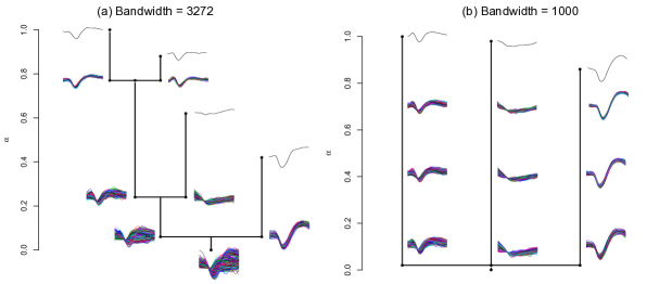
Figure 5: Conformal trees for the neuron data. (a): conformal tree with bandwidth $h$ chosen to maximize the variance of $\widehat{p}_{h}(X_{1}),...,\widehat{p}_{h}(X_{n})$ and $\epsilon$ set to $0.5\times\max\{\min_{X_{i},X_{j}\in\widehat{\cal C}_{n,\alpha}}d(X_{i},X_{j})\}$. (b): conformal tree obtained using: $h=\epsilon=1000$. The plots show the clusters for different values of $\alpha$. Next to each node (e.g., split), we plot the curves belonging to the elements of the corresponding partition of $\widehat{\cal C}_{n,\alpha}$. Isolated clusters of size smaller than 10 are ignored.

5 Conclusion and Future Directions

We have extended conformal methods and its variants to functional data. Using the inductive conformal predictor, together with basis projections, we obtain the first distribution-free simultaneous prediction bands for functional data with finite sample performance guarantee. These prediction bands can also be viewed as quantile sets of the underlying process that corresponding to high density region. On the other hand, using standard conformal prediction with pseudo densities, the prediction set ${\cal C}_{n}$ also reveals hierarchical and salient features in the data. We have proposed methods for extracting information from and visualizing ${\cal C}_{n}$. Currently, we are investigating several open questions such as extension of the new conformal method to other conformity scores in high dimensional problems and issues regarding optimality and the selection of tuning parameters. For functional data, the choice of distance in pseudo densities is also interesting. It can be shown that for the $L_{2}$ distance, the induced bands are unbounded. The results using the distance $d^{2}(f,g)=\sum_{j}e^{\gamma j}(\beta_{j}-\theta_{j})^{2}$ for example are somewhat different (not shown). Here, $\{\beta_{j}\}$ and $\{\theta_{j}\}$ are the coefficients $f$ and $g$ in the cosine basis. We call this the analytic distance as it is related to the set of analytic functions; see page 46 of Efromovich (1999). This distance is much more sensitive to the shape of the curve.

References

- Antoniadis et al. (2010) Antoniadis, A., Xavier Brossat, J. C., & Poggi, J. (2010). Clustering functional data using wavelets. In e-book of COMPSTAT, (pp. 697–704). Springer.
- Cheng (1995) Cheng, Y. (1995). Mean shift, mode seeking, and clustering. Pattern Analysis and Machine Intelligence, IEEE Transactions on, 17(8), 790–799.
- Cuevas et al. (2007) Cuevas, A., Febrero, M., & Fraiman, R. (2007). Robust estimation and classification for functional data via projection-based depth notions. Computational Statistics, 22, 481–496.
- Delaigle et al. (2012) Delaigle, A., Hall, P., & Bathia, N. (2012). Componentwise classification and clustering of functional data. Biometrika, 99.
- Efromovich (1999) Efromovich, S. (1999). Nonparametric curve estimation: methods, theory and applications. Springer Verlag.
- Febrero et al. (2008) Febrero, M., Galeano, P., & González-Manteiga, W. (2008). Outlier detection in functional data by depth measures, with application to identify abnormal nox levels. Environmetrics, 19.
- Ferraty & Vieu (2006) Ferraty, F., & Vieu, P. (2006). Nonparametric functional data analysis: theory and practice. Springer Verlag.
- Gervini (2009) Gervini, D. (2009). Detecting and handling outlying trajectories in irregularly sampled functional datasets. The Annals of Applied Statistics, 3, 1758–1775.
- Hartigan (1975) Hartigan, J. (1975). Clustering Algorithms. John Wiley, New York.
- Hastie et al. (2009) Hastie, T., Tibshirani, R., & Friedman, J. (2009). The Elements of Statistical Learning. Springer, 2nd ed.
- Hyndman & Shang (2010) Hyndman, R. J., & Shang, H. L. (2010). Rainbow plots, bagplots, and boxplots for functional data. Journal of Computational and Graphical Statistics, 19, 29–45.
- James & Sugar (2003) James, G. M., & Sugar, C. A. (2003). Clustering for sparsely sampled functional data. Journal of the American Statistical Association, 98, 397–408.
- Lei et al. (2013) Lei, J., Robins, J., & Wasserman, L. (2013). Efficient nonparametric conformal prediction regions. Journal of the American Statistical Association. To appear.
- Lei & Wasserman (2013) Lei, J., & Wasserman, L. (2013). Distribution free prediction bands for nonparametric regression. Journal of the Royal Statistical Society: Series B (Statistical Methodology). To appear.
- López-Pintado & Romo (2009) López-Pintado, S., & Romo, J. (2009). On the concept of depth for functional data. Journal of the American Statistical Association, 104, 718–734.
- Ramsay & Silverman (1997) Ramsay, J., & Silverman, B. (1997). Functional Data Analysis. New York: Springer.
- Rinaldo et al. (2012) Rinaldo, A., Singh, A., Nugent, R., & Wasserman, L. (2012). Stability of density-based clustering. Journal of Machine Learning Research, 13, 905–948.
- Rinaldo & Wasserman (2010) Rinaldo, A., & Wasserman, L. (2010). Generalized density clustering. The Annals of Statistics, 38, 2678–2722.
- Rousseeuw et al. (1999) Rousseeuw, P. J., Ruts, I., & Tukey, J. W. (1999). The bagplot: a bivariate boxplot. The American Statistician, 53, 382–387.
- Shafer & Vovk (2008) Shafer, G., & Vovk, V. (2008). A tutorial on conformal prediction. Journal of Machine Learning Research, 9, 371–421.
- Shi & Wang (2008) Shi, J., & Wang, B. (2008). Curve prediction and clustering with mixtures of gaussian process functional regression models. Statistics and Computing, 18, 267–283.
- Sun & Genton (2011) Sun, Y., & Genton, M. G. (2011). Functional boxplots. Journal of Computational and Graphical Statistics, 20, 216–334.
- Tarpey & Kinateder (2003) Tarpey, T., & Kinateder, K. K. J. (2003). Clustering functional data. Journal of Classification, 20, 93–114.
- Vovk et al. (2005) Vovk, V., Gammerman, A., & Shafer, G. (2005). Algorithmic Learning in a Random World. Springer.
- Yao et al. (2005) Yao, F., Müller, H.-G., & Wang, J.-L. (2005). Functional data analysis for sparse longitudinal data. Journal of the American Statistical Association, 100(470), 577–590.