A decomposition technique for pursuit evasion games with many pursuers

Abstract

Restrictions on memory storage impose ultimate limitations on the dimensionality of differential games problems for which optimal strategies can be computed via direct solution of the associated Hamilton-Jacobi-Isaacs equations. It is of interest therefore to explore whether, for certain specially structured differential games of interest, it is possible to decompose the original problem into a family of simpler, lower dimensional, differential games. In this paper we exhibit a class of single pursuer-multiple evader games for which a reduction in complexity of this nature is possible. The target set is expressed as a union of smaller, sub-target, sets. The individual differential games in the family are obtained from the original problem by taking as target set an element in the family of sub-target sets, in place of the original target set. We can exploit geometric features of the dynamic constraints and constraints of the problems arising in this way to reformulate them as lower dimensional, simpler to solve, problems. We give conditions under which the value function of the original can be characterized as the lower envelope of the value functions for the simpler problems and how optimal strategies can be constructed from those for the simpler problems. The methodology is illustrated by several examples.

I Introduction

Interest in Pursuit-Evasion differential games (PE games) involving several players dates back to the 1960’s. Progress in this field is documented in the classical differential games literature, which includes the books by Isaacs [11], Pontryagin [15], Friedman [8], Krasovskii and Subbotin [14]. Constructing optimal strategies for each player, finding the value of the game, deriving optimality conditions for the trajectories and establishing conditions for solvability of the game are typical objectives.

The case of several agents, although it can be considered as a special case of the general framework for the problem, has been addressed separately by many authors. An early significant contribution was that of Pshenichnii [16], who studied the problem with many pursuers and equal speeds and derived necessary and sufficient conditions for solutions to this problem. Ivanov and Ledyaev [12] subsequently studied the optimal pursuit in higher dimensional state spaces, with several pursuers and geometrical constraints. Through the study of an auxiliary problem, related to the interaction between one pursuer and the evader and using a Lyapunov function, they obtained sufficient conditions of optimality. Chodun [4] and more recently Ibragimov [10] used the same approach to solve a collection of one to one problems (one pursuer one evader) for problems with simple dynamic constraints.

Differential games, and multi-agent PE games in particular, have found applications in a variety of fields, for example in mathematical economics, where a game has been constructed to model the relation between agents [13, 6], in robotics where typically the emphasis is real time solutions and efficient computational methods. [9, 17].

Our proposed approach is to decompose the original game into a family of simpler, lower-dimensional games. This is achieve by expressing the original set as a union of smaller, target subsets. The individual differential games in the family result from the replacing the original target set by each of the target subsets. Special geometric features of the dynamic constraints and constraints can be exploited to reduce the complexity of the new problems generated in this way. Making use of verification techniques originally proposed by Isaacs [5, 2], properties of viscosity solutions and techniques of nonsmooth analysis [1, 3], we give we a lower-envelope characterization of the value function, and show how to construct optimal strategies for the original problem from those for the simpler problems. A similar decomposition technique was used in [7].

II The Hamilton-Jacobi-Isaacs approach to pursuit-evasion games

The state $y$ of a dynamic system, partitioned as $n$-vector components $y=(y_{1},\ldots,y_{m})$, is governed by the equations

$$\begin{array}[]{l}y_{1}^{\prime}(t)=-g_{1}(y(t))a_{1}(t)+h_{1}(y(t))b(t)+l_{1}(y(t))\\ \vdots\\ y_{m}^{\prime}(t)=-g_{m+1}(y(t))a_{m}(t)\\ \hskip 65.04256pt+h_{m}(y(t))b(t)+l_{m}(y(t))\;.\end{array}$$ (1)

in which $g_{i}(.),h_{i}(.):\mathbb{R}^{n}\rightarrow\mathbb{R}$, $i=1,\ldots,m+1$ and $l_{i}(.):\mathbb{R}^{n}\rightarrow\mathbb{R}^{n}$ are given functions.

For each $i$ we interpret the state component $y_{i}$ to be the relative position of the evader with respect to the $i$’th pursuer. The dimension of the state vector $y$ is therefore $N=n\times m$. The $n\times m$ vector $a=(a_{1},\ldots,a_{m})$ comprises the $n$-vector pursuer controls and $b$ is the $n$-vector evader control.

The pursuer and evader controls $a$ and $b$ take values in the sets

$$\begin{array}[]{l}A=B_{n}(0,\rho_{a})\times\ldots\times B_{n}(0,\rho_{a}),\quad B=B_{n}(0,\rho_{b})\\ \end{array}$$ (2)

for some given numbers $\rho_{a},\,\rho_{b}>0$. Define

$$\mathcal{A}:=\{\mbox{ meas. functions }a:[0,+\infty)\rightarrow A\}$$ (3)

$$\mathcal{B}:=\{\mbox{ meas. functions }b:[0,+\infty)\rightarrow B\}$$ (4)

It is assumed that

(H): $g_{i}(.),h_{i}(.),l_{i}(.)$, $i=1,\ldots m+1$ are Lipschitz continuous, and

$g_{i}(x)\rho_{a}-h_{i}(x)\rho_{b}-|l_{i}(x)|>0,\quad\forall x\in\mathbb{R}^{N},\quad\forall i$.

Note that the maximum allowable magnitude of the velocity of the $i$’th pursuer depends on the states of all the pursuers and the evader, via the functions $g_{i}(.)$, $h_{i}(.)$ and $l_{i}(.)$. We may assume, without loss of generality that the $g_{i}$’s and $h_{i}$’s are positive functions, since the constraint sets $A$ and $B$ are symmetric about the origin.

Take the target set to be

$$\mathcal{T}=\{(y_{1},y_{2},...,y_{m})\in\mathbb{R}^{N}:\min_{i\in\{1,2...m\}}|y_{i}|\leq r\}\,,$$ (5)

in which $r\geq 0$ is a specified number. Denote by $y_{x}(.)=y_{x}(.,a,b)$ the solution of (1), for given initial state $x$ and controls $a(.)\in{\cal A}$ and $b(.)\in{\cal B}$. Define the hitting time for (given $x$, $a$ and $b$) to be

$$t_{x}(a,b):=\left\{\begin{array}[]{l}\min\{t:y_{x}(t;a,b)\in\mathcal{T}\}\\ +\infty\quad\hbox{if }y_{x}(t;a,b)\notin\mathcal{T}\;\forall t.\end{array}\right.$$ (6)

The player with control $a$ (comprising the pursuers) seeks to minimize the hitting time, while the evader player, with control $b$, seeks to maximize it. It is convenient to transform the hitting time cost by means of the mapping

$$\psi(u):=\left\{\begin{array}[]{ll}1-e^{-u}&\hbox{if }u<+\infty\\ 1&\hbox{if }u=+\infty\;.\end{array}\right.$$ (7)

The cost becomes:

$$J(x,a,b)=\psi(t_{x}(a,b))=\int_{0}^{t_{x}}e^{-s}ds.$$ (8)

The transformation modifies the value function, but leaves unaltered the optimal strategies, owing to the fact that the transformation is monotone.

Full specification of the differential game requires precise description of the nature of the control strategies involved. For this purpose, we follow the Elliot/Kalton approach, based on the concept of ‘non-anticipative’ strategies. The set of such strategies for the $a$-player is

$$\Gamma:=\{\alpha:\mathcal{B}\rightarrow\mathcal{A}:t>0,b(s)=\tilde{b}(s)\hbox{ for all }s\leq t\\ \hbox{ implies }\alpha[b](s)=\alpha[\tilde{b}](s)\hbox{ for all }s\leq t\}\;.$$ (9)

$$\Delta:=\{\beta:\mathcal{A}\rightarrow\mathcal{B}:t>0,a(s)=\tilde{a}(s)\hbox{ for all }s\leq t\\ \hbox{ implies }\beta[a](s)=\beta[\tilde{a}](s)\hbox{ for all }s\leq t\}\;.$$ (10)

The upper and lower values of the game are

$$u^{+}(x):=\sup_{\beta\in\Delta}\inf_{a\in\mathcal{A}}J(x,a,\beta[a])$$

$$u^{-}(x):=\inf_{\alpha\in\Gamma}\sup_{b\in\mathcal{B}}J(\alpha[b],b)\;.$$

Under the stated hypotheses, and in view of the fact the Isaac’s condition is satisfied, the upper and lower values coincide, for arbitrary initial state $x$. The common value defines the value function $u(.)$ for the game. Thus $u(x)=u^{+}(x)=u^{-}(x)$ for all $x$.

It can be shown that, under the state assumptions, the value function is the unique uniformly continuous function $u(.):\mathbb{R}^{N}\rightarrow\mathbb{R}$, which vanishes on on ${\cal T}$ and which is a viscosity solution on $\mathbb{R}^{N}\backslash{\cal T}$ of the following Hamilton-Jacobi-Isaacs equation

$$\left\{\begin{array}[]{ll}u(x)+H(x,Du(x))=0&x\in\mathbb{R}^{N}\setminus\mathcal{T}\\ u(x)=0&x\in\partial\mathcal{T}\end{array}\right.$$ (11)

where The Hamiltonian is

$$H(x,p=(p_{1},\ldots,p_{m}))\;=$$

$$\,\rho_{a}\sum_{i=1}g_{i}(x)|p_{i}|-\rho_{b}|\sum_{i=1}h_{i}(x)p_{i}|$$

$$\hskip 72.26999pt-\sum_{i=1}l_{i}(x)\cdot p_{i}-1\;.$$

Furthermore, the value function is locally Lipschitz continuous.

Solving this equation for the value function of the game, yields the optimal strategy of each player for initial state $x_{0}$ as $a(t)=S(y_{x_{0}}(t))$ and $b(t)=W(y_{x_{0}}(t))$ where

$S(z)\in\underset{a\in A}{\operatorname{argmax}}\,\underset{b\in B}{\min}\{(g(x)a-h(x)b-l(x))\cdot Dv(x)\}$

$W(z)\in\underset{b\in B}{\operatorname{argmin}}\,\underset{a\in A}{\max}\{(g(x)a-h(x)b-l(x))\cdot Dv(x)\}.$

Example 1. We examine a simple, preliminary example. Consider the pursuit-evasion game with two pursuers $p_{1},p_{2}$ and one evader $e$, and the positions of each evolve in 1D space. We take the dynamics to be

$$\left\{\begin{array}[]{l}p_{1}^{\prime}=\frac{2}{3}a_{1}\\ p_{2}^{\prime}=a_{2}\\ e^{\prime}=\frac{b}{2}\\ p_{1}(0)=p_{1}^{0}\\ p_{2}(0)=p_{2}^{0}\\ e(0)=e^{0}\end{array}\right.$$ (12)

where $a_{1},a_{2},b\in B(0,1)=[-1,1]$, $p_{1},p_{1},e\in\mathbb{R}$. The speed constraint on pursuers is assumed to be greater than that of the evader; this ensures that the optimal hitting time is finite for an arbitrary initial finite state.

Let us now consider a reduced formulation. We translate the origin to the position of the e-player, so the $i$’th state variable becomes the position of the evader relative to that of the $i$’th pursuer. There results the reduced dynamics

$$\left\{\begin{array}[]{l}y_{1}^{\prime}=-\frac{2}{3}a_{1}+\frac{b}{2}\\ y_{2}^{\prime}=-a_{2}+\frac{b}{2}\\ y_{1}(0)=p_{1}^{0}-e^{0}\\ y_{2}(0)=p_{2}^{0}-e^{0}\end{array}\right.$$ (13)

here we have $a_{1},a_{2},b\in B(0,1)$, $y_{1},y_{2}\in(-\infty,+\infty)$. The target set $\mathcal{T}$ becomes the union of neighbourhoods the two axes: capture occurs when $\min_{i\in\{1,2\}}|p_{i}-e|\leq r$, for some specified $r\geq 0$.

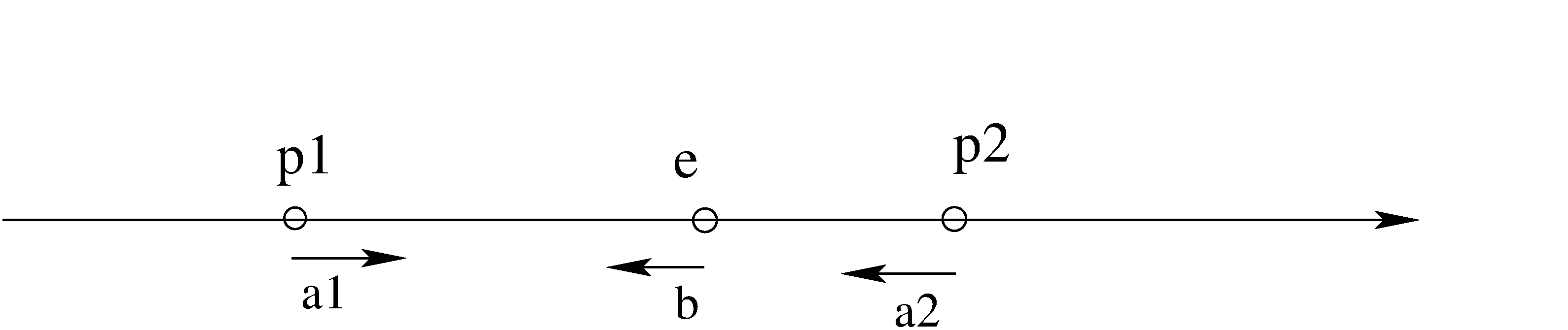
Figure 1: A monodimensional PE game with two pursuers.

The HJI equation is

$$\left\{\begin{array}[]{l}u(x)+\max\limits_{a_{1},a_{2}}\min\limits_{b}\left\{(\frac{2}{3}a_{1}-\frac{b}{2},a_{2}-\frac{b}{2})\cdot Du(x)\right\}=1\\ \hskip 101.17755ptx\in[0,+\infty]^{2}\setminus\mathcal{T}\\ u(x)=0\hskip 65.04256pt\par x\in\partial\mathcal{T}\end{array}\right.$$ (14)

Observe that, with this formulation, the dimension of the domain in which we seek to solve (14) is two. The rapid growth in complexity of the problem with increase in the number of the pursuers places severe restrictions on the computability of this equation for state dimensions greater than three. We now propose a decomposition technique to address this challenge.

III A decomposition technique for the $m$ pursuer problem

In this section we present a decomposition technique to overcome the complexity of the multiple pursuer game introduced in Section 2, for high state dimensions. The key idea is to decompose the target set ${\cal T}$ as a union of smaller sets ${\cal T}_{i}$, $i=1,\ldots,m$:

$$\mathcal{T}_{i}=\{(y_{1},y_{2},...,y_{m})\in\mathbb{R}^{N}:|y_{i}|\leq r\},\;i=1,\ldots,m.$$ (15)

and to relate the value function $u(.)$ for the original game to the value functions $u_{i}(.)$ for the games in which the ${\cal T}_{i}$’s replace ${\cal T}$. The $u_{i}(.)$’s are viscosity solutions to the HJI equation above, with modified boundary condition:

$$\left\{\begin{array}[]{ll}u_{i}(x)+H\left(x,Du_{i}(x)\right)=0&x\in\mathbb{R}^{N}\setminus\mathcal{T}_{i}\\ u_{i}(x)=0&x\in\mathcal{T}_{i}\end{array}\right.$$ (16)

Under the hypotheses, the $u_{i}(.)$’s are Lipschitz continuous.

Define the index set

$$I(x)\,:=\,\{i\in\{1,\ldots,m\}:u_{i}(x)=\min_{i}u(i)\}\;.$$

Theorem III.1

Assume condition (C) is satisfied:

(C): for arbitrary $x\in\mathbb{R}^{N}\backslash{\cal T}$, any convex combination $\{\lambda_{i}\,|\,i\in I(x)\}$ and any collection of vectors $\{\xi_{i}\in\partial^{L}u_{i}(x)\,|\,i\in I(x)\}$ we have

$$H(x,\sum_{i}\lambda_{i}\xi_{i})\,\leq\,\sum_{i\in I(x)}\lambda_{i}H(x,\xi_{i})\,.$$ (17)

Then

$$u(x)\;=\;\underset{i}{\min}\{u_{1}(x),\ldots,u_{m}(x)\}\,$$

for all $x\in\mathbb{R}^{N}\backslash{\cal T}$.

Remark III.2

Here the limiting superdifferential $\partial^{L}u_{i}(x)$ is the set

$$\partial^{L}u_{i}(x)\;:=\;\underset{x^{\prime}\rightarrow x}{\mbox{lim sup}}\;\partial^{F}u_{i}(x)\;,$$

in which $\partial^{F}u_{i}(x)$ is the super Frechet differential

$\quad\partial^{F}u_{i}(x)\,=\,$

$\{p\in\mathbb{R}^{N}:\underset{x^{\prime}\rightarrow x}{\mbox{lim sup}}\,\frac{u_{i}(x^{\prime})-u_{i}(x)-p\cdot(x^{\prime}-x)}{|x^{\prime}-x|}\leq 0\}\,.$

Condition (C) is automatically is satisfied if $H(x,.)$ is a convex function, but is in fact significantly weaker.

Proof Outline. Define

$$\overline{u}(x):=\min\{u_{i}(x);i\in 1\ldots m\}\quad\mbox{for all }x$$ (18)

Our aim is to show that $\overline{u}(.)$ coincides with $u(.)$. Since $\overline{u}(.)$ vanishes on ${\cal T}$, and in view of the facts that $\overline{u}(.)$ is Lipschitz continuous and that $u(.)$ is the unique uniformly continuous viscosity solution to the HJI equation satisfying this boundary condition, it suffices to show that $\overline{u}(.)$ is such a solution.

That $\overline{u}(.)$ is a super (viscosity) solution follows directly from the definition of super solution and the fact that $\overline{u}(.)$ is the lower envelope of a finite number of super solutions. It remains to show then that $\overline{u}(.)$ is a sub solution. Take any $x\in\mathbb{R}^{N}\backslash{\cal T}$ and any $\xi\in\partial^{F}(x)$. According to a well-known characterization of sub solutions, it suffices to demonstrate that

$$\overline{u}+H(x,\xi)\,\leq\,0\;.$$ (19)

But, by the ‘max rule’ for limiting subdifferentials of Lipschitz continuous functions, applied to $-\overline{u}(x)=\underset{i}{\max}(-u)(x)$, we know that, for some convex combination $\{\lambda_{i}\,|\,i\in I(x)\}$ and set of vectors $\{\xi_{i}\in\partial^{L}u_{i}(x)\,|\,i\in I(x)\}$.

$$\xi=\underset{i\in I(x)}{\sum}\lambda_{i}\xi_{i}\;.$$

For each $i\in I(x)$, there exists sequences $x^{i}_{j}\rightarrow x$ and $\xi^{i}_{j}\rightarrow\xi_{i}$ such that, for each $i$, $\xi\in\partial^{F}(x^{i}_{j})$ as $j\rightarrow\infty$. Since $u_{i}(.)$ is a subsolution, $H(x^{i}_{j},\xi^{i}_{j})\leq 0$. But then, since $H(.,.)$ is continuous,

$$H(x,\xi_{i})\leq\underset{j}{\mbox{lim sup}}\,H(x^{i}_{j},\xi^{i}_{j})\,\leq 0\,$$

It follows from condition (17) that

$$H(x,\xi)\,=\,H(x,\underset{i}{\sum}\lambda_{i}\xi_{i})\,\leq\,\underset{i}{\sum}\lambda_{i}H(x,\xi_{i})\;.$$

then

$$\overline{u}+H\left(x,\sum_{i}\lambda_{i}p_{i}\right)\leq\sum_{i}\lambda_{i}\overline{u}+\sum_{i}\lambda_{i}H(x,p_{i})\\ \leq\sum_{i}\lambda_{i}\left(u_{i}+H(x,p_{i})\right)\leq 0.$$ (20)

We have confirmed (19).                               $\square$

We now discuss the role the decomposition technique, summarized as Theorem III.1, in reducing the complexity of the differential game.

Consider again Example 1. The target can be expressed as a union of two sets: $\mathcal{T}:=\mathcal{T}_{1}\cup\mathcal{T}_{2}$, in which $\mathcal{T}_{i}:=\{(x_{1},x_{2})\in\mathbb{R}^{2}:|x_{i}|\leq r\}$. For the target $\mathcal{T}_{1}$ (respectively $\mathcal{T}_{2}$), the value function is clearly independent of $x_{2}$ (respectively $x_{1}$). So $\frac{\partial}{\partial x_{2}}u_{1}(x_{1},x_{2})=0$ and $\frac{\partial}{\partial x_{1}}u_{2}(x_{1},x_{2})=0$. $u_{1}(.)$ therefore satisfies

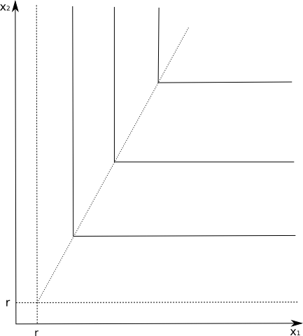
Figure 2: Some level sets for the value function of the monodimensional problem with two pursuers

$$\left\{\begin{array}[]{l}u_{1}+\max\limits_{a_{1}}\min\limits_{b}\left\{-(-\frac{2}{3}a_{1}+\frac{b}{2})\cdot\frac{\partial}{\partial x_{1}}u_{1}\right\}=1\\ \phantom{ffvvvtttttfffff}x_{1}\in(r,+\infty],x_{2}\in[0,+\infty)\\ u_{1}=0\phantom{fvvfffff}x_{1}\in[0,r],x_{2}\in[0,+\infty)\end{array}\right.$$ (21)

where $a_{1}\in B_{n}(0,\rho_{a})$ and $b\in B_{n}(0,\rho_{b})$. This is a 1D equation for a fixed $\overline{x}_{2}$ and is constant for a fixed $\overline{x}_{1}$. It has solution

$$u_{1}(x)=1-e^{-6(x_{1}-r)}\hbox{, }\psi^{-1}(u_{1})=6(x_{1}-r)$$ (22)

Similarly

$$u_{2}(x)=1-e^{-2(x_{2}-r)}\hbox{, }\psi^{-1}(u_{2})=2(x_{2}-r)\;.$$ (23)

The gradients of these two functions at $x$ are of the form $(k_{1}(x),0)$, $(0,k_{2}(x))$ for non-negative functions $k_{1}(.)$ and $k_{2}(.)$. It is simple to check that condition (C) is satisfied. According to Thm. III.1, the value function as lower envelope of $u_{1}(.)$ and $u_{2}(.)$, thus

$$\psi^{-1}(\overline{u})=\left\{\begin{array}[]{ll}-6(x_{1}-r)&\hbox{if }x_{1}\leq\frac{1}{3}x_{2}+\frac{2}{3}r\\ -2(x_{2}-r)&\hbox{if }x_{1}>\frac{1}{3}x_{2}+\frac{2}{3}r.\end{array}\right.$$ (24)

Remark III.3

These optimal strategies are consistent with intuition. When one pursuer is very close to the evader, that pursuer’s location alone affects the strategy of the evader, as expected. This feature of the solution is evident from the formulae for the value function, which reveal that, for states far from the $x_{1}$ axis but close to the $x_{2}$ (for example), the value function coincides with the function $u_{i}(x)$.

The preceding analysis can be generalized to cover a unidimensional problem with $m$ pursuers.

Theorem III.4

Assume hypotheses (H). Denote by $v_{i}(.):\mathbb{R}\rightarrow\mathbb{R}$ the solution of the following equation

$$\left\{\begin{array}[]{l}v_{i}(x_{i})+\max\limits_{a_{i}}\min\limits_{b}\left\{f_{i}(x_{i},a_{i},b)\cdot Dv_{i}(x_{i})\right\}=1\\ \phantom{tttppppppppppppppppppppttttttttttt}x_{i}\in(r,+\infty]\\ v(x_{i})=0\phantom{gggggggggggggggggggggg}x_{i}\in[0,r]\end{array}\right.$$

where $f_{i}(x_{i},a_{i},b):=g_{i}(x)a_{i}-h_{i}(x_{i})b-l(x_{i})$, $a_{i}\in B_{1}(0,\rho_{a})$, $b\in B_{1}(0,\rho_{b})$.

$$u_{i}(x=(x_{1},x_{2}...x_{i},...x_{m}))=v_{i}(x_{i})$$

Then the value function $u(.)$ is

$$u(x)\;=\;\min\{u_{1}(x),\ldots,u_{m}(x)\}$$

Proof:

It is straightforward to confirm that $u_{i}(x)$ is a viscosity solution of the problem (16), using the fact that $\frac{\partial u_{i}}{\partial x_{j}}(x)=0$ for all $i\neq j$. Then, in view of the uniqueness of viscosity solutions for (16) ([1] Theorem 3.1), we know that $u_{i}(.)$ is the unique viscosity solution of the decomposed problem $\eqref{P1}$.

Making use of the fact that that $\xi_{i}\in\partial^{L}u_{i}(x)$ has the structure $(0,\ldots,0,k_{i},0,\ldots,0)$, where $k_{i}\geq 0$, we deduce Then, for any $\xi_{i}\in\partial^{L}u_{i}(x)$ and $\xi_{j}\in\partial^{L}u_{j}(x)$ with $i,j\in I(x)$, we have

$$H(x,\xi_{i}+\xi_{j})=\\ \rho_{a}\left(g_{i}|k_{i}|+g_{j}|k_{j}|\right)-\rho_{b}|h_{i}k_{i}+h_{j}k_{j}|-l_{i}\cdot(0...k_{i}...k_{j}...0)\\ =\left(\rho_{a}g_{i}|k_{i}|-\rho_{b}|h_{i}k_{i}|-l_{i}\cdot(0...k_{i}...0)\right)\\ +\left(\rho_{a}g_{j}|k_{j}|-\rho_{b}|h_{j}k_{j}|-l_{j}\cdot(0...k_{j}...0)\right)\\ =H(x,\xi_{i})+H(x,\xi_{j}).$$ (25)

this confirms condition (C) of Thm. III.1 is satisfied. The stated characterization of the value function now follows from Thm. III.1. ∎

IV Examples and numerical tests.

In this section we solve some higher dimensional problems using the proposed decomposition technique. We note that memory storage constraints impose fundamental limits on the state dimensions of problems for which solutions to the associated HJI equations can be computed directly. Indeed, MATLAB implementations using a heap-based Java VM system are not feasible for $N$ dimensional arrays, for $N>5$ . This provides the motivation for studying decomposition techniques which are, in principle, applicable for very high dimensional problems.

Test 1

In this example we study pursuit-evasion game on a plane involving several pursuers and one evader, with the help of Thm. 3.1.

Consider the problem in a reduced space where the variable $x_{i}$ is the distance between the evader and the $i$’th pursuer and every pursuer has constant maximum speed $g_{i}(x)\equiv 1$. The evader has constant maximum speed $\displaystyle h_{i}(x)=0.9$.

The $i$’th unidimensional problem is, for control constraint sets $a_{i}\in B_{1}(0,1)$ and $b\in B_{1}(0,1)$, has associated HJI equation

$$\left\{\begin{array}[]{l}v_{i}(x_{i})+\min\limits_{a_{i}}\max\limits_{b}\left\{(g_{i}a_{i}-h_{i}(x)b)\cdot D_{i}v_{i}(x_{i})\right\}=1\\ \phantom{gggggggggggggggggggggggggg}x_{i}\in(r,+\infty]\\ v(x_{i})=0\phantom{gggggggggggggggggg}x_{i}\in[0,r].\end{array}\right.$$ (26)

We extend now the $v_{i}$ solution in the space of dimension 5: $V_{i}(x):\mathbb{R}^{5}\rightarrow R$ is defined as

$$u_{i}(x=(x_{1},...x_{i},...x_{5}))=v_{i}(x_{i})\;.$$ (27)

The value function of the problem is simply

$$u(x)=\min\{u_{1}(x),\ldots,u_{5}(x)\}.$$ (28)

Figs. 3, 4 we show simulations for two different with different starting points.

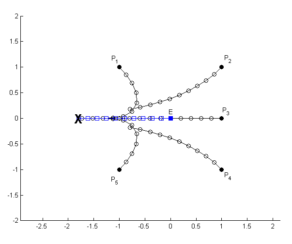
Figure 3: Test 1: optimal trajectories at various times. A $X$ indicates the point of capture.

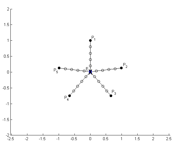
Figure 4: Test 1: optimal trajectories at various times. A $X$ indicates the point of capture. The optimal trajectory of the evader is waiting the capture.

Test 2

In this example, we consider a PE game involving several pursuers and one evader, but now in presence of an obstacle (a river, a different kind of medium) which affects the velocities of the pursuers and the evader. In this case we cannot pass to the reduced coordinates, since this will result in a loss of the information about the position of the agents. Accordingly, the first $m$ block components of the state are associated with the pursuers and the $(m+1)$’th block component with the evader. The positions of the agents, evolving in $\mathbb{R}^{n}$, are governed by the following equations

$$\left\{\begin{array}[]{l}y_{1}^{\prime}(t)=-g(y(t))a_{1}(t)\\ y_{2}^{\prime}(t)=-g(y(t))a_{2}(t)\\ \ldots\\ y_{m}^{\prime}(t)=-g(y(t))a_{m}(t)\\ y_{m+1}^{\prime}(t)=h(y(t))b(t)\,,\end{array}\right.$$ (29)

where the state $y:=(y_{1}^{T},y_{2}^{T},...,y_{m+1}^{T})^{T}\in\mathbb{R}^{N}$ and every $y_{i}\in\mathbb{R}^{n}$. We assume that $g:\mathbb{R}^{n}\rightarrow\mathbb{R}^{+}$ and $h:\mathbb{R}^{n}\rightarrow\mathbb{R}^{+}$, so every pursuer has the same velocity rule (depending from the position; in the previous case $y$ was the distance between agents). This will give us a geometric property which will guarantee the decomposability of the problem. The appropriate target set in the present setting is

$$\mathcal{T}=\left\{(y_{1}^{T},y_{2}^{T},...,y_{m+1}^{T})\in\mathbb{R}^{N}:\right.\\ \left.\min_{i\in\{1,2...m\}}|y_{i}-y_{m+1}|\leq r\right\}$$ (30)

Fig. 5 illustrates the target set in the case $m=2$, $n=1$.

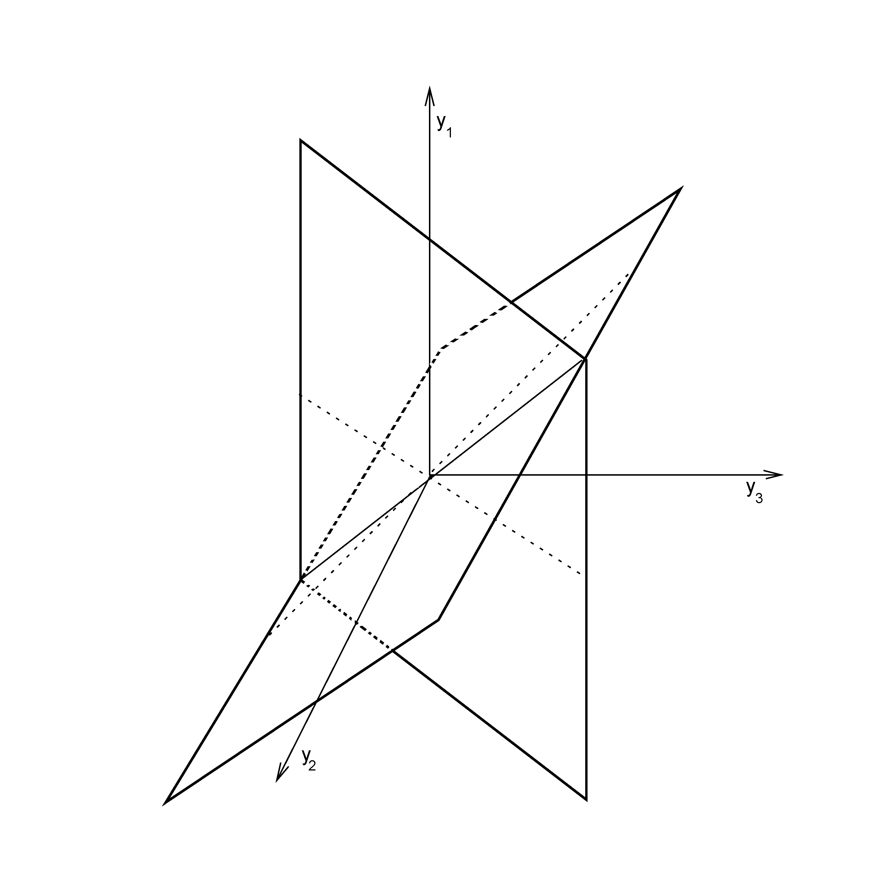
Figure 5: Test 2: Target set for $m=2$, $n=1$, $r=0$.

The Hamiltonian, which is

$$H(x,p)=g(x)\sum_{i=1}^{m}\rho_{a}|p_{i}|-h(x)\rho_{b}|p_{m+1}|-1\,,$$

is not convex in the $p$ variable.

Theorem IV.1

Assume (1), (2). Let $u_{i}(.):\mathbb{R}^{n}\rightarrow\mathbb{R}$ the solution of the following equation

$$\left\{\begin{array}[]{l}v_{i}(x_{i})+\max\limits_{a_{i}}\min\limits_{b}\left\{(g(x_{i})a_{i},-h(x)b)\cdot Dv_{i}(x_{i})\right\}=1\\ \phantom{ggggggggggggggggggggggg}x\in(r,+\infty]^{2n}\\ v(x_{i})=0\phantom{gggggggggggggggg}x_{i}\in\{|x_{1}-x_{2}|\leq r\}\end{array}\right.$$ (31)

with $a_{i}\in B_{n}(0,\rho_{a})$, $b\in B_{n}(0,\rho_{b})$. Define the function $u_{i}(x):\mathbb{R}^{N}\rightarrow\mathbb{R}$ as

$$u_{i}(x=(x_{1},\ldots,,x_{m}))=v_{i}(x_{i})\;.$$ (32)

Then the value function for the original problem is

$$u(x)=\min\{u_{1}(x),\ldots,u_{m}(x)\}$$

Proof:

To simplify the notation, suppose that $n=1$. (The case for a general $n$ is treated in the same way). We can see that the Hamiltonian is convex in $p$ along rays in every direction with exception of the $e_{m+1}$ direction. (Here, $e_{i}$ is $i$’th canonical basis vector).

We can repeat the main steps in the proof of Theorem III.4 with the exception of the verification of condition $(C)$. In this case we know, for geometric reason, the superdifferential of the function $u(.)$ is an element aligned with $e_{m+1}$, i.e.

$$\xi_{i},\xi_{j}\in\partial^{F}u(x),\quad(\xi_{i}-\xi_{j})\cdot e_{m+1}=0.$$

This follows from the fact that $e_{m+1}$ is tangential to the switching interface. Writing $u_{i}$ and $u_{j}$ for two reduced value functions, we can show that $u_{i}(.)=u_{j}(.)$, i.e. they solve the same equation. It follows that the switching interface is located where two reduced value functions coincide, i.e. where $u_{j}(x)=u_{i}(x)$. Writing $n$ for the normal of the switching interface, we have

$$n\cdot e_{m+1}=\left(0,\ldots,0,\frac{\partial u_{i}}{\partial x_{i}},0,\ldots,0,\frac{\partial u_{i}}{\partial x_{j}},0,\ldots,0\right)^{t}\\ \cdot\left(0,\ldots,0,1\right)^{t}=0\;.$$ (33)

Condition $(C)$ can now be validated. the state representation of $u(.)$ is therefore valid by Thm. 3.1. ∎

As an example, consider the $n=2$ case. An evader has position denoted by $x_{e}\in\mathbb{R}^{2}$ and $m\in\mathbb{N}$ pursuers have positions denoted by $x_{1},x_{2},...x_{n}\in\mathbb{R}^{2}$. Take $m=3$. It is assumed that

$$\left\{\begin{array}[]{ll}g(x)=1-0.5\cos(\pi x)&\hbox{ if }|x_{2}|<0.5\\ g(x)=1&\hbox{elsewhere}\end{array}\right.$$ (34)

and $h(x)\equiv 0.4$.

Figs. 6, 7 show some optimal trajectories and the level sets of the velocity function of the pursuers.

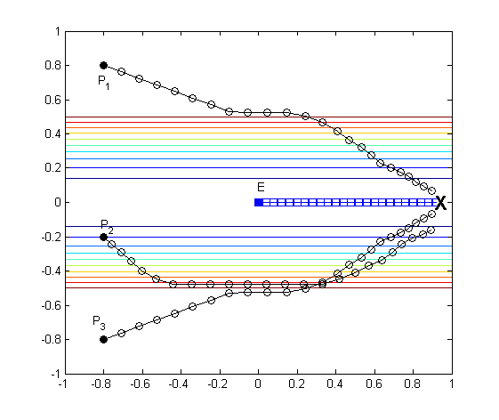
Figure 6: Test 2: optimal trjectories for a 3pursuers game.

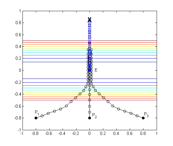
Figure 7: Test 2: optimal trjectories for a 3pursuers game.

V ACKNOWLEDGMENTS

This work was supported by the European Union under the 7th Framework Programme FP7-PEOPLE-2010-ITN SADCO, Sensitivity Analysis for Deterministic Controller Design.

References

- [1] M. Bardi and I. Capuzzo-Dolcetta, Optimal Control and Viscosity Solution of Hamilton-Jacobi-Bellman Equations. Birkhauser, Boston Heidelberg 1997.
- [2] M. Bardi, T.E.S. Raghavan, T. Parthasarathy, Stochastic and Differential Games: Theory and Numerical Methods, Birkhauser, Boston Heidelberg, 1999.
- [3] P. Cannarsa and C. Sinestrari. Semiconcave functions, Hamilton-Jacobi equations, and optimal control, Birkhauser, Boston Heidelberg, 2004.
- [4] W. Chodun, Differential games of evasion with many pursuers, J. Math. Anal. Appl. 142 (1989), no. 2, 370–389.
- [5] R.J. Elliott and N.J. Kalton. Values in differential games. Bull. Amer. Math. Soc. Vol. 78, No 3 (1972), 427–431.
- [6] G.M. Erickson, A differential game model of the marketing-operations interface, Eur. J. Oper. Res. 211 (2011) 294–402.
- [7] P. Falugi, C. Kountouriotis and R. Vinter, Differential Games Controllers That Confine a System to a Safe Region in the State Space, With Applications to Surge Tank Control, IEEE T. Automat. Contr. (2012) 57(11): 2778-2788 .
- [8] A. Friedman, Differential Games, John Wiley & Sons, New York, USA, 1971.
- [9] J.Hu and M. Wellman. Multiagent Reinforcement Learning: Theoretical Framework and an Algorithm. Proceedings of ICML, (1998) 242-250.
- [10] G.I. Ibragimov, Optimal pursuit of an evader by countably many pursuers. Differ. Equ. 41 (2005), no. 5, 627–-635.
- [11] R. Isaacs, Differential Games, John Wiley & Sons, New York, USA, 1965.
- [12] R.P. Ivanov and Yu. S. Ledyaev, Time optimality for the pursuit of several objects with simple motion in a differential game. Trudy Mat. Inst. Steklov. 158 (1981), 87–97.
- [13] S. Jørgensen, Optimal production, purchasing and pricing: A differential game approach, Eur. J. Oper. Res. 24 (1) (1986) 64–76.
- [14] N.N. Krasovskii and A.I. Subbotin, Game-Theoretical Control Problems, Springer, New York, 1988.
- [15] L.S. Pontryagrin, Izbrange Trudy (Selected works), Moskow, Russia, 1988.
- [16] B.N. Pshenichnii, Simple pursuit by several objects, Cybern. Syst. Anal. 12 (3) (1976) 484–485.
- [17] R. Vidal, O. Shakernia, J. Kim, Associate Member, H. Shim, S.Sastry, Probabilistic Pursuit–Evasion Games: Theory, Implementation, and Experimental Evaluation, IEEE T. Robotic. Autom., (2002) Vol. 18, No. 5.