A phenomenological approach to the equation of state of a unitary Fermi gas

Abstract

We propose a phenomenological approach for the equation of state of a unitary Fermi gas. The universal equation of state is parametrised in terms of Fermi-Dirac integrals. This reproduces the experimental data over the accessible range of fugacity and normalised temperature, but cannot describe the superfluid phase transition found in the MIT experiment [4]. The most sensitive data for compressibility and specific heat at phase transition can, however, be fitted by introducing into the grand partition function a pair of complex conjugate zeros lying in the complex fugacity plane slightly off the real axis.

1 Introduction

Recently, the thermodynamics of a unitary gas of fermionic atoms has been in the focus of experimental investigations [1, 2, 3, 4]. In a unitary gas, the inter-atomic interaction between neutral fermionic atoms is adjusted using the Feshbach resonance [5], so that the scattering length goes to $\pm\infty$. Such a gas has properties that are universal or scale independent [6]. The experimental confirmation of the universal nature of the equation of state (EOS) of a gas of neutral fermionic atoms has therefore given fresh impetus to its theoretical understanding [7, 8]. In a recent paper [9], an ansatz for the grand potential of a spin balanced two-component fermion gas was introduced through a virial expansion in powers of the fugacity variable $z$. This ansatz for the interaction part of the virial coefficients could fit the experimental data up to about $z=7$, surprising in view of the fact that it was meant to be a high temperature expansion for small $z$. For $z>7$, i.e., at low temperatures, the virial expansion was found to become unphysical.

In this paper we propose a novel phenomenological approach to describe the EOS, that agrees with experimental data all the way to very low temperatures and reproduces some of the zero temperature properties quantitatively. Following Sommerfeld [10], it would seem that at low temperatures when $z\gg 1$, $x=\ln z$ is a more suitable expansion parameter. Since a unitary gas introduces no extra length scales than already present in the ideal gas, we go one step further and express the grand potential in terms of a simple combination of two Fermi-Dirac integrals [11]. This allows us to fit the experimental data quite accurately, and at the same time to reproduce the correct second virial coefficient at small $z$, i.e., for high temperatures.

Furthermore, experimentally, a phase transition to super-fluidity is observed around $T/T_{F}\simeq 0.16$, evidenced by peaks in the heat capacity and compressibility [4]. To reproduce these features in our model, we introduce a phenomenological term in the grand partition function, which in the zero-width limit yields a singularity in the free energy and hence describes a phase transition.

In Sec. II, we first introduce our new phenomenological ansatz and show that it reproduces the universal function $h(z)$, which is the ratio of pressures of the spin-balanced two-component unitary gas and free Fermi gas, over a large range of experimentally available fugacities $z$. In Sec. III, we compute all the thermodynamic quantities for which experimental data are available and show that our phenomenological ansatz indeed incorporates the essential features of the data.

2 The phenomenological equation of state

The grand potential $\Omega$ of the unitary gas is related to the grand partition function ${\cal Z}$ by the thermodynamical relation

$$\Omega=-PV=-k_{B}T\ln{\cal Z}\,,$$ (1)

where $P$ and $V$ are pressure and volume, respectively, $T$ is the temperature, and $k_{B}$ the Boltzmann constant. The grand partition function is defined by

$${\cal Z}(\beta,z)=\sum_{N=0}^{\infty}Z_{N}(\beta)\,z^{N},\qquad\beta=1/k_{B}T\,,$$ (2)

where $Z_{N}(\beta)$ is the canonical $N$ particle partition function. Note that in the above series, the dependences on $\beta$ and $z$ are mixed. However, for the ideal free Fermi gas, ${\cal Z}$ has the form

$$\ln{\cal Z}_{F}(\beta,z)=\frac{V}{\lambda^{3}}\,2f_{5/2}(z)\,,\quad\lambda=\left(\frac{2\pi\hbar^{2}\beta}{m}\right)^{\!\!1/2}\!,$$ (3)

in which the $z$ dependence has separated out and is entirely coming through the function $f_{5/2}(z)$ which is one of the Fermi-Dirac integrals defined [11] as

$$f_{\nu}(x)=\frac{1}{\Gamma(\nu)}\int_{0}^{\infty}\frac{y^{(\nu-1)}dy}{1+e^{(y-x)}}\,.$$ (4)

For a unitary gas, a similar separation of variables $\beta$ and $z$ also takes place [6]. We therefore define a universal function $F_{P}(z)$ by

$$\ln{\cal Z}(\beta,z)=(V/\lambda^{3})\,F_{P}(z)\,.$$ (5)

In terms of this function, we define the universal thermodynamic function $h(z)$ by

$$h(x)=\frac{\Omega}{\Omega_{F}}=\frac{P}{P_{F}}=\frac{F_{P}(x)}{2f_{5/2}(x)}\,,\qquad x=\ln(z)\,,$$ (6)

where $\Omega_{F}$ and $P_{F}$ are the grand potential and pressure of the untrapped ideal Fermi gas, respectively. Note that in this quantity the dependence on temperature and length scales drops out, so that it is universal and scale independent (see also [1]).

The all-important function $F_{P}(x)$ encodes the thermodynamic properties of the unitary gas of fermionic atoms. We make the important assumption that $F_{P}(x)$ can be written as a linear superposition of Fermi-Dirac integrals since this ensures universality. Thus we introduce the function $F_{P}(x)$ through the following phenomenological ansatz:

$$F_{P}(x)=2[f_{5/2}(x)+4(f_{5/2}(x)-f_{3/2}(x))]+g(x)\,,$$ (7)

where the factor 2 in front accounts for spin degeneracy. This ansatz is further guided by the following considerations:

1. The function $h(x)$ obeys universality, i.e., it depends only on the fugacity $z=\exp(x)$, but not on any length scale or other system variable.

2. The leading term $f_{5/2}(x)$ in Eq. (7) is simply that of the free non-interacting Fermi gas given in Eq. (3).

3. The second term $4(f_{5/2}(x)-f_{3/2}(x))$ describes the contribution from the interactions. By definition this term does not contribute to the linear term in $z$ in the high temperature expansion of $F_{P}(x)$ (cf. [11]). Furthermore, the linear superposition of Fermi-Dirac integrals is determined to yield the exact interaction part of the second virial coefficient $\Delta b_{2}$ [12] in the high temperature limit. This choice, however, does not yield the correct third virial coefficient that is known to great accuracy, nor the estimated fourth virial coefficient [13, 14]. Nevertheless, the high temperature properties that we obtain still give excellent agreement with experimental results. On the other hand, the zero temperature properties are entirely determined by the function $f_{5/2}(x)$. The overall factor 5 of $f_{5/2}(x)$ allows for a good description also of the zero temperature properties of the unitary gas (see the detailed discussion to Fig. 2 below).

4. The function $g(x)$ in Eq. (7), which is implicitly a function of the fugacity $z=\exp(x)$, is introduced in order to describe the phase transition that has been observed in the experimental data [4]. For this purpose, we write the grand partition function ${\cal Z}$ in the complex $z$ plane as

$${\cal Z}={\widetilde{\cal Z}}\left[\left(1-\frac{z}{z_{c}+i\epsilon}\right)\!\left(1-\frac{z}{z_{c}-i\epsilon}\right)\right]^{(V/\lambda^{3})},$$ (8)

with real $z_{c}$ and $\epsilon$, where ${\widetilde{\cal Z}}$ describes the system without phase transition. At $z=z_{c}\pm i\epsilon$, this function goes to zero, causing a logarithmic singularity of the free energy in the limit $\epsilon\to 0$. The power $(V/\lambda^{3})$ of the zeros is required to preserve the universality of $h(x)$. For the function $g(z)$, which is found through Eqs. (7) and (5), this yields

$$g(z)=\ln\left[\frac{(z_{c}-z)^{2}+\epsilon^{2}}{z_{c}^{2}+\epsilon^{2}}\right]+2\,\frac{z}{z_{c}}\,.$$ (9)

The last term in Eq. (9) is introduced such that $g(x)$ gives no contribution to the first-order virial coefficient in the high temperature (i.e., small-$z$) expansion of $F_{P}(x)$. The choice of $z_{c}$ and $\epsilon$ is guided by a fit to the experimental data on compressibility and specific heat: while $z_{c}$ is given by the critical temperature of the phase transition, $\epsilon$ is governed by the width of the transition region.

We find that $z_{c}=13.5$ and $\epsilon=6.3$ give the best fits to the MIT data for compressibility and specific heat, seen in Fig. 3 below. While the form (9) of $g(x)$ works well throughout the phase transition region and all the way to small $z$ (i.e., to high temperatures), it becomes unphysical in the zero $T$ limit where we are forced to use the ansatz (7) with $g=0$.

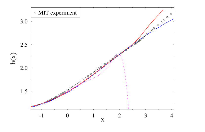
Figure 1: (Colour online) The function $h(x)$ for the untrapped unitary Fermi gas as a function of $x=\ln(z)$. The crosses represent the experimental MIT data by Ku et al [4]. Our result including the full $g(x)$ in (7) is shown by the (red) solid line. The result obtained by putting $g(x)=0$ is shown by the (blue) dashed line. We also show the results for the virial ansatz [9] by the (magenta) dotted line.

In Fig. 1 we compare our numerical results with the experimental data of the MIT group [4] for the universal function $h(x)$ given in Eq. (6). The solid line corresponds to the full expression (7) for $F_{P}(x)$, while the dotted line is obtained using $g(x)=0$. We see that the our phenomenological ansatz closely follows the data up to $x\sim 2.5$, while the high temperature virial ansatz introduced in [9] fails much earlier. For large $x$, the results obtained with $g(x)=0$ and with $g(x)$ given in (9) lie on either side of the data, the solid line showing that $g(x)$ becomes unphysical for $x>3$. In all calculations presented henceforth, we have put it to zero for $z>z_{max}=27$, corresponding to $x_{max}=3.3$ and a temperature $T_{min}=0.1\,T_{F}$, below which there are essentially no data points found in the figures below.

3 Thermodynamical properties

Encouraged by the good agreement over a large range of $x$ for our universal function $h(x)$, we now consider the calculation of basic thermodynamic observables. Following Ku et al. [4], we write for the normalised pressure

$$\widetilde{p}=\frac{P}{P_{0}}=\frac{5T}{2T_{F}}\frac{F_{P}(x)}{F^{\prime}_{P}(x)}=\frac{5}{3}\frac{E}{NE_{F}}\,,$$ (10)

where $P$ and $E$ are pressure and energy, respectively, of the interacting gas. The quantities used for the normalisation in the denominators above are all evaluated for the non-interacting gas: $P_{0}$ is the pressure at zero temperature, $T_{F}$ the Fermi temperature, and $E_{F}$ the Fermi energy; the latter two are related by $E_{F}=k_{B}T_{F}$. The prime here and below denotes derivative with respect to $x$. The normalised temperature is given by

$$\frac{T}{T_{F}}=\frac{k_{B}T}{E_{F}}=\frac{4\pi}{[3\pi^{2}F^{\prime}_{P}(x)]^{2/3}}\,.$$ (11)

The entropy, also related to pressure, is given by

$$\frac{S}{Nk_{B}}=\frac{T_{F}}{T}\left(\widetilde{p}-\frac{\mu}{E_{F}}\right)=\frac{5F_{P}(x)}{2F^{\prime}_{P}(x)}-\ln(z)\,.$$ (12)

The chemical potential $\mu$, normalised with respect to the non-interacting Fermi energy $E_{F}$, is given by

$$\frac{\mu}{E_{F}}=\widetilde{p}-\frac{TS}{T_{F}Nk_{B}}\,.$$ (13)

Analogously, the normalised compressibility is given by

$$\widetilde{\kappa}=\frac{\kappa}{\kappa_{0}}=\frac{2T_{F}}{3T}\frac{F^{\prime\prime}_{P}(x)}{F^{\prime}_{P}(x)}\,.$$ (14)

The specific heat at constant volume is given by

$$\frac{C_{V}}{Nk_{B}}=\frac{15}{4}\frac{F_{P}(x)}{F^{\prime}_{P}(x)}-\frac{9F^{\prime}_{P}(x)}{4F^{\prime\prime}_{P}(x)}=\frac{3T_{F}}{2T}\left(\tilde{p}-\frac{1}{\tilde{\kappa}}\right).$$ (15)

We note that both compressibility and specific heat depend on the second derivatives of the function $F_{P}(x)$.

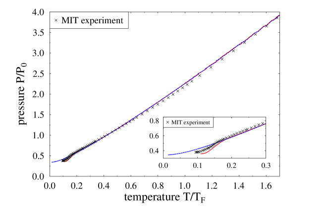
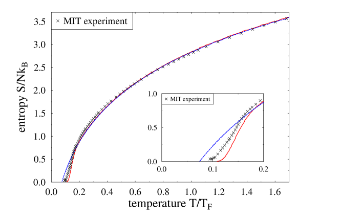
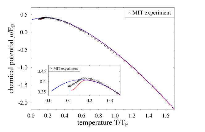
Figure 2: (Colour online) Normalised pressure (top), entropy (middle) and chemical potential (bottom) of the unitary Fermi gas as a function of temperature. The crosses denote the experimental MIT data [4]. Dashed (blue) and solid (red) lines are as in Fig. 1. The inserts give enlarged pictures of the low-temperature domain including the phase transition region.

We now present numerical results for the thermodynamic quantities for which experimental data are available. Since no ready-to-use numerical routines for the Fermi-Dirac integrals $f_{\nu}(x)$ could be found, we have calculated them by numerical integration of Eq. (4). This is easily possible to any desired accuracy for $\nu>1$. For $\nu\leq 1$ we employed the formula [11] $f_{\nu-1}(x)=f^{\prime}_{\nu}(x)$ and used numerical differentiation to obtain $f^{\prime}_{\nu}(x)$.

In Fig. 2 we compare our results of normalised pressure (top), entropy (middle), and chemical potential (bottom) with the MIT data. Our ansatz describes all these data quite well all the way down to the critical temperature $T_{c}=0.16\,T_{F}$. At high temperatures the results are comparable to, if not better than, the virial ansatz discussed in Ref. [9]. Departures are noticed around critical temperature $T_{c}$ (enlarged in the inserts). Like in Fig. 1, the results with and without including $g(x)$ lie on opposite sides of the data below $T_{c}$; the solid lines do reproduce the kink seen in the chemical potential at $T=T_{c}$.

We stress again that in Eq. (7) with $g(x)=0$, only the contribution $2\times 5f_{5/2}(x)$ is relevant for reproducing the results at $T=0$. For the energy per particle at $T=0$ it yields $E/N=(3/5){\widetilde{E}}_{F}$, where ${\widetilde{E}}_{F}$ if the Fermi energy of the interacting gas. Further, it is easily deduced that ${\widetilde{E}}_{F}/E_{F}=\xi=(1/5)^{2/3}=0.342$, which is slightly less than the experimentally determined value 0.36 of the MIT experiment [4]. We emphasise that our fit of $h(x)$ (see Fig.2) is particularly sensitive to the linear combination of $f_{5/2}$ and $f_{3/2}$ used in our ansatz (7), which was primarily chosen to yield a reasonable high temperature limit. Any different choice of parameters, or any admixture of Fermi-Dirac integrals $f_{\nu}$ with other orders $\nu$, could not simultaneously yield both these desirable large- and zero-temperature limits.

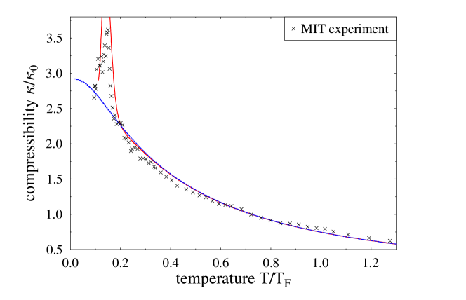
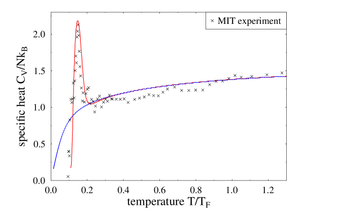
Figure 3: (Colour online) Normalised compressibility (top) and specific heat (bottom) of the unitary Fermi gas as functions of temperature (crosses and lines as in the previous figures).

In Fig. 3 we show the results of our calculation for compressibility (top) and specific heat (bottom) as functions of temperature. The resonant term $g(x)$ in $F_{P}(x)$ here gives an excellent description of the experimental peaks seen in both quantities. Again, it has to be cut at $T<T_{min}=0.1\,T_{F}$, and the result obtained with $g(x)=0$ yields the correct limits ${\widetilde{\kappa}}(T$=$0)=1/\xi$ and $C_{V}(T$=$0)=0$. In Fig. 4 we finally plot compressibility versus normalised pressure like it was done in Ref. [4]. Note here, in particular, the excellent agreement with the data up to the highest available pressures.

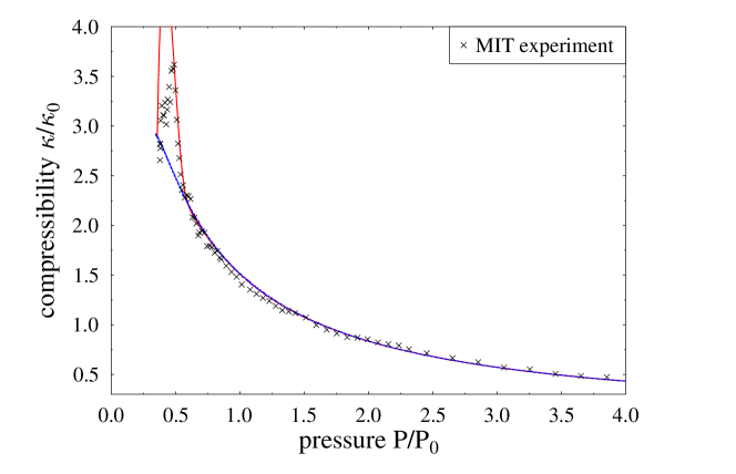
Figure 4: (Colour online) Normalised compressibility versus normalised pressure (crosses and lines as in the previous figures).

4 Summary and conclusions

To summarise, we have introduced a phenomenological function $F_{P}(x)$, given by Eq. (7) that yields the universal equation of state (6) of a unitary fermion gas. $F_{P}(x)$ depends solely on the fugacity $z$ (or on $x=\ln z$) and hence is scale independent. It consists of two Fermi-Dirac integrals, $f_{5/2}(x)$ and $f_{3/2}(x)$, and a resonant term $g(z)$ that corresponds to a pair of zeros of the grand partition function in the complex $z$ plane, suitable for describing the phase transition observed in the experiments. The non-resonant Fermi-Dirac part of $F_{P}(x)$ is constructed to yield a reasonable high temperature limit by imposing the value $\Delta b_{2}=1/\sqrt{2}$ of the second virial coefficient [12]; it contains otherwise no adjustable parameter. As a bonus, it also yields zero temperature limits that fit the data. The only two parameters $z_{c}$ and $\epsilon$, appearing in Eq. (9) for the resonant term $g(x)$, have been fitted to the critical temperature $T_{c}=0.16\,T_{F}$ and the width of the phase transition found in the MIT data for specific heat and compressibility (see Fig. 3). The function $g(z)$ diverges for $z\to\infty$, i.e., for $T\to 0$. It was therefore put to zero for $z>z_{max}=27$ corresponding to $T<T_{min}=0.1\,T_{F}$. However, the available data seen in the Figures 2 - 4 are lying at $T>T_{min}$, so that we can claim to describe all these data with our full ansatz (7). The only sizeable deviation is found in Fig. 1 for the quantity $h(x)$ which appears to have been measured even below $T_{min}$, and for which our results including $g(x)$ take off already above $T_{min}$. Nevertheless, we can claim that our ansatz, in spite of its simplicity, describes the overall experimental data surprisingly well. To construct it, we have mainly used the universal properties of a gas at unitarity, as well as crucial experimental observations.

It is also tempting to extend the above analysis for trapped fermionic atoms at unitarity. Following the arguements given above we may write $F_{P}^{(trap)}(x)$ in the form

$$F_{P}^{(trap)}(x)=2[f_{4}(x)+4(f_{4}(x)-f_{3}(x))]+g^{(trap)}(x)\,,$$ (16)

which is similar in form to the ansatz given in 7, with the Fermi integrals of the gas replaced by the appropriate Fermi integrals for the trap. In the first part there are no new parameters and the second virial coefficient is reproduced correctly. This form also determines the zero temperature properties of trapped fermionic system at unitarity. However, in the absence of data on compressibility and specific heat it is not possible to determine the second term $g(x)^{(trap)}$ and thus the full form of the thermodynamic potential. Nevertheless, the form suggested above may be useful in analysing the results for the trap also in future.

It would be interesting to see if our $F_{P}(x)$ can be obtained from a microscopic model. We have not succeeded with this, but it is hoped that our analysis will trigger future investigations in this direction.

References

References

- [1] S. Nascimbène, N. Navon, K. J. Jiang, F. Chevy, and C. Salomon, Nature 463, 1057 (2010).
- [2] N. Navon, S. Nascimbène, F. Chevy, and C. Salomon, Science 328, 729 (2010).
- [3] M. Horikoshi, S. Nakazima, M. Ueda, and T. Mukaiyama, Science 327, 442 (2010).
- [4] M. J. H. Ku, A. T. Sommer, L. W. Cheuk, and M. W. Zwierlein, Science 335, 563 (2012).
- [5] H. Feshbach, Ann. Phys. (N.Y.), 5, 537 (1958).
- [6] T.-L. Ho, Phys. Rev. Lett. 92, 090402 (2004).
- [7] H. Hu, X,-J. Liu, and P. D. Drummond, New Journal of Physics 12, 063038 (2010).
- [8] H. Hu, X,-J. Liu, and P. D. Drummond, Phys. Rev. A 83, 063610 (2011).
- [9] R. K. Bhaduri, W. van Dijk and M. V. N. Murthy, Phys. Rev. Lett. 108, 260402 (2012).
- [10] A Sommerfeld, Zeitschrift für Physik 47, 1 (1928).
- [11] R. K. Pathria, Statistical Mechanics (Pergamon Press, 1972) Appendix E, p. 508.
- [12] T.-L. Ho and E. J. Mueller, Phys. Rev. Lett. 92, 160404 (2004).
- [13] X.-J. Liu, H. Hu, and P. D. Drummond, Phys. Rev. Lett. 102, 160401 (2009).
- [14] D. Rakshit, K. M. Daily, and D. Blume, Phys. Rev. A 85, 033634 (2012).