Coalescence of Pickering emulsion droplets induced by electric-field

Abstract

Combining high-speed photography with electric current measurement, we investigate the electrocoalescence of Pickering emulsion droplets. Under high enough electric field, the originally-stable droplets coalesce via two distinct approaches: normal coalescence and abnormal coalescence. In the normal coalescence, a liquid bridge grows continuously and merges two droplets together, similar to the classical picture. In the abnormal coalescence, however, the bridge fails to grow indefinitely; instead it breaks up spontaneously due to the geometric constraint from particle shells. Such connecting-then-breaking cycles repeat multiple times, until a stable connection is established. In depth analysis indicates that the defect size in particle shells determines the exact merging behaviors: when the defect size is larger than a critical size around the particle diameter, normal coalescence will show up; while abnormal coalescence will appear for coatings with smaller defects.

When two droplets come into contact, they naturally coalesce to minimize the surface energy, a phenomenon extensively studied since 19th century thomson ; duchemin ; aartsjfm ; caseprl ; casepre . A quite recent study reveals that coalescence starts from the regime controlled by inertial, viscous, and surface-tension forces pnas , which is followed by either a viscous regime aartsprl or an inertial regime zaleski . However, the coalescence of special droplets – Pickering emulsion droplets – remains poorly understood. Stabilized by colloidal particles instead of surfactant molecules, Pickering emulsions are composed by particle-coated droplets Ramsden ; pickering , as shown in Fig.1a. Due to the highly controllable permeability, mechanical strength and biocompatibility velev ; dinsmore ; lee , Pickering emulsions have been actively studied in the last decade, and may find broad applications in important areas such as oil recovery eow and drug-delivery simovic . The well-controlled coalescence in Pickering emulsions can also facilitate material mixing and benefit the field of chemical and biochemical assays Ahn . More interestingly, the existence of an extra structure – particle shell – may bring fundamentally different merging physics and enrich the classical coalescence research. Consequently, there is great scientific and practical significance to clarify the coalescence of Pickering emulsion droplets.

If the surface is poorly coated, droplets can coalesce spontaneously and form supracolloidal structures Subramaniam ; andrea . Complex dynamics and structure of particles are observed during coalescence, due to the combined effects of charge, surface tension and liquid flow fuller . Numerical simulation further reveals that the repulsion between particles, the particles’ ability to attach to both droplet surfaces, and the stability of the liquid film between droplets are crucial for coalescence behaviors alberto . However, if the surface is coated by closely packed particles, coalescence rarely occurs. Inspired by the strong influence of electric field, which can deform liquid surface into conical tips taylor ; brazier ; stone ; basaran , create liquid jets out of these tips basaran , induce electrocoalescence between two isolated droplets brazier or among a large population of droplets basaran2 , and even prevent droplets from coalescing bird ; ristenpart ; we thus apply high voltage between two Pickering emulsion droplets and investigate their coalescence under electric field. The originally-stable droplets coalesce systematically, via two distinct approaches: normal coalescence and abnormal coalescence. In the first approach, a liquid bridge grows continuously and merges two droplets together, similar to the classical picture. In the second approach, however, completely different behaviors emerge: a liquid bridge forms through defects but fails to grow indefinitely; instead it breaks up spontaneously due to the geometric constraint from particle shells. Such connecting-then-breaking cycles repeat multiple times, until a stable connection is established. Further analysis indicates that the defect size in particle shells determines the exact merging behaviors: when defects are larger than a critical size, the normal approach will show up; while the abnormal coalescence will occur for smaller defects. This study generalizes the understanding of coalescence to a more complex system.

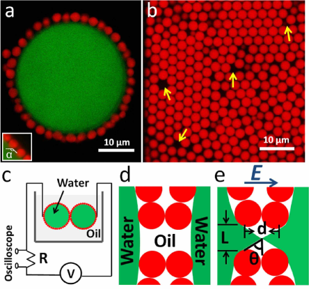
Figure 1: (color online). (a) The 2D confocal slice of a typical Pickering emulsion droplet. The saltwater droplet is dyed in green and the PMMA particles are dyed in red. The particles have the diameter $d=3\mu m$ for this particular sample. The magnified image in the inset shows the contact angle of particles at the interface: $\alpha=133\pm 5^{\circ}$. (b) The arrangement of particles in the shell. The yellow arrows point to some typical defects. (c) Diagram of the experimental setup. A DC voltage is applied through two electrodes that are in direct contact with the droplets. The current between two droplets is recorded by an oscilloscope. (d) A cartoon illustrating the separation of water droplets without electric field. (e) With high enough electric filed, a liquid bridge is formed through defects. $d$ is particle diameter, $L$ is the defect size, and $\theta$ is the cone angle.

We make Pickering emulsions by suspending saltwater droplets (12.5 wt% NaCl) in the organic solvent decahydronaphthalene (DHN). The droplets are stabilized by Poly(methyl methacrylate) (or PMMA) particles of diameter $d$. To ensure the general robustness of the results, we vary $d$ from $0.3\mu m$ to $3\mu m$ in the experiment. The emulsion droplets have the typical size of a few millimeters. One such droplet is illustrated by confocal microscopy in Fig.1a, with the internal saltwater fluorescently labeled in green and the PMMA particles dyed in red. Apparently, particles coat the droplet surface, forming a protective shell velev ; dinsmore . The magnified image in the lower inset shows the contact angle of particles at the interface: $\alpha=133\pm 5^{\circ}$. Fig.1b focuses on the particle shell: most particles are closely packed in the shell, with some defects randomly distributed irvine , as indicated by the arrows. These defects play an important role in coalescence, as demonstrated later by our study.

We directly visualize the merging of millimeter-size droplets with a fast camera (Photron SA4), at the frame rate of $10,000s^{-1}$. A DC electric voltage is applied through two electrodes that are in direct contact with the droplets (see Fig.1c). We gradually increase the voltage until coalescence takes place. To probe microscopic events the fast camera can not resolve, we further measure the electric current between the two droplets with an oscilloscope caseprl ; casepre . The current measurement is sensitive to any tiny connection at the beginning of coalescence. The time resolution of this approach is determined by the relaxation time of charging process in our salt solution and has the typical value of $\tau\sim 10^{-10}s$ footnote . These two approaches (high-speed photography and electric current) are synchronized to reveal a complete picture at both the macroscopic and the microscopic levels. The sketch of the system is shown in Fig.1c.

When electric field is absent or small, two contacting droplets never coalesce in our experiment, due to the protection of particle shells. However, sufficiently strong electric field can induce conical tip structures at the droplet surface taylor ; basaran ; stone , which may penetrate through the large pores of defects and form a connection, as demonstrated by the cartoon in Fig.1e. To simplify the analysis and illustrate the underlying physics, we assume that the defects in the two shells have identical size and align perfectly. We define the particle diameter as $d$, the defect size as $L$, and the the cone angle as $\theta$ bird . The electric field applies a local electrical stress, $\Sigma_{E}\sim\epsilon\epsilon_{0}E_{loc}^{2}$, onto the interface. Once $\Sigma_{E}$ exceeds the restoring capillary pressure, $P_{cap}\sim\gamma/L$, significant deformation will occur and a liquid bridge may form. Here $\epsilon\epsilon_{0}$ is the permittivity of the oil, $E_{loc}$ is the local electric field around the defect, and $\gamma$ is the surface tension of the water-oil interface. Apparently, the local electric field must exceed a finite value, $E_{loc}\sim\sqrt{\gamma/(\epsilon\epsilon_{0}L)}$, to establish a connection.

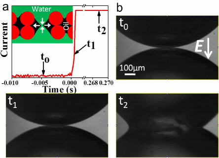
Figure 2: (color online). (a) The electric current between two droplets during a normal coalescence. Before connection, the signal fluctuates about zero (see $t=t_{0}$). Around $t=t_{1}$, however, it rises rapidly and saturates the apparatus, revealing the establishment of a stable connection. Inset cartoon illustrates the widening of the connection by the water flow. (b) The corresponding images from the synchronized fast photography. At $t_{0}=-4.7ms$, the droplets are intact. At $t_{1}=0.5ms$, although a connection is suggested by the electric signal, its small size prevents the direct observation. Significant variation in profile only occurs long after the connection, as illustrated at $t_{2}=268.8ms$. The voltage between two droplets is $50V$ for this particular event.

Once connected, the liquid bridge may continuously widen and merge the two droplets, as illustrated by the cartoon of Fig.2a (see the supplemental movie S-1 for real situation). The main panel of Fig.2a plots the electric current signal from oscilloscope. At $t=t_{0}$, no connection is established and the signal fluctuates about zero. Around $t=t_{1}$, however, the signal rises sharply and saturates the apparatus, indicating the formation of a stable connection. We define the starting point of this sharp rise as time zero throughout our measurements. The three typical moments, $t_{0}=-4.7ms$, $t_{1}=0.5ms$, and $t_{2}=268.8ms$, are illustrated by the high-speed images in Fig.2b. Clearly, the connection at $t_{1}$ barely changes the macroscopic picture, showing the limitation of photography and the essence of electrical measurements. Significant change in profile is only observed long after the connection, as demonstrated by the image at $t_{2}=268.8ms$.

The entire process lasts several hundred milliseconds, much longer than the water droplet coalescence without particle shells ($\sim 1ms$) aartsprl . We also notice that coalescence may stop in the middle and never reach the state shown in the $t_{2}$ image. These behaviors are caused by the particle shells, within which jammed particles can slow down or even terminate coalescence andrea .

More interestingly, a completely different merging process – abnormal coalescence – is observed. The behaviors of the electric signal is shown in Fig.3a: instead of increasing monotonically to saturate the oscilloscope, the signal exhibits multiple peaks, as demonstrated by the ones at $t_{1}$ and $t_{3}$. Fig.3b plots the zoomed-in details of one particular peak, and Fig.3c shows the corresponding images from synchronized photography.

The high-speed images reveal the detailed dynamics during abnormal coalescence: due to electrical attraction, the two droplets approach each other, flattening the contact area but failing to merge, as shown by the $t_{0}$ image in Fig.3c. In the subsequent development, however, the two droplets repeatedly approach then move away from each other, making multiple oscillatory-like cycles (see the supplemental movie S-2). Surprisingly, these cycles coincide exactly with the major peaks in the electric signal, as illustrated in Fig.3b: the rapid-rising of signal around $t_{2}$ corresponds to the approaching of droplets, the local maximum at $t_{3}$ matches the moment of closest distance between two droplets, and the sharp-declining part around $t_{4}$ agrees with the moving away of two droplets. Similar cycles repeat multiple times, until a stable connection is reached, as illustrated in the circle of the $t_{5}$ image. For this particular experiment, coalescence stops at this point, due to the particle jamming inside the shells.

These observations suggest the following picture for each cycle: the electric field deforms the droplet surfaces and establishes a connection through large pores, as illustrated in Fig.1e. This connection then quickly broadens, increasing the electric signal and pulling two droplets together. However, after reaching a maximum thickness, the bridge shrinks and breaks up, reducing the current to zero value; correspondingly the two droplets move away from each other, possibly due to the elastic repulsion from particle shells.

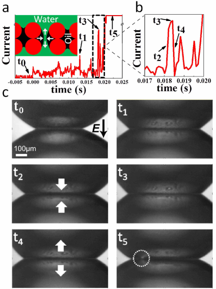
Figure 3: (color online). (a) The electric current signal for an abnormal coalescence. From no connection at $t_{0}$ to the stable connection at $t_{5}$, the signal exhibits multiple cycles of peaks, such as the ones at $t_{1}$ and $t_{3}$. The inset cartoon illustrates the narrowing of the neck due to the outward water flow, which breaks the bridge and completes one peak cycle. (b) The zoomed-in picture for one particular peak at $t_{3}$. The signal rises sharply around $t_{2}$, reaches maximum at $t_{3}$, and drops dramatically around $t_{4}$. (c) The corresponding images from the synchronized fast photography. At $t_{0}$, there is no connection but the contact area is flattened due to the electric attraction. The image at $t_{1}$ corresponds to one peak in the electric signal. Images $t_{2}$ through $t_{4}$ clarify the particular peak shown in (b). Around $t_{2}$, the droplets approach each other as indicated by the arrows, and corresponds to the sharp rise of the electric signal. At $t_{3}$, two droplets are at the closest distance and the signal reaches the maximum. Around $t_{4}$, the droplets move away from each other, and agrees with the dramatic drop of signal. The image of $t_{5}$ shows a stable connection inside the circle. The specific times are: $t_{0}=1.3ms,t_{1}=13.1ms,t_{2}=18.0ms,t_{3}=18.4ms,t_{4}=18.6ms$, and $t_{5}=22.2ms$. The voltage between two droplets is $80V$.

The direct visualization of liquid bridge would serve as an ideal confirmation for the above picture. However it typically occurs within the contact area and eludes such observation. After a number of trials, nevertheless, we successfully catch the cycles of bridge formation and break-up with fast camera, as shown in Fig.4a: no connection exists at $t_{0}$, while a tiny bridge is formed at $t_{1}$ (inside the box), which subsequently breaks up at $t_{2}$. Comparing with the electric signal in Fig.4b, we find an exact correspondence between the moment of bridge formation in Fig.4a and the peak location in Fig.4b at $t=t_{1}$. Similar cycles appear for many times (see the supplemental movie S-3 for a clear demonstration), and the correspondence between bridge formation and signal peak is always observed. These findings unambiguously verify our picture of the abnormal coalescence.

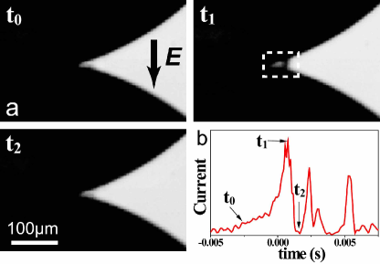
Figure 4: (color online). (a) The direct visualization of a liquid bridge. No connection exists at $t_{0}=-2.5ms$, while a tiny bridge is formed at $t_{1}=1.0ms$ (inside the box), which subsequently breaks up at $t_{2}=2.0ms$. (b) The corresponding electric signal. Clearly the bridge formation in (a) coincides exactly with one particular peak in the electric signal.

One essential question remains unclear: why does the bridge shrink and break up, instead of growing continuously? We propose a geometric explanation similar to the non-coalescence mechanism of charged water droplets bird ; ristenpart . Because of particle shells, the droplet surfaces are separated by a fixed distance around the particle diameter, $d$. Thus the geometry of the bridge depends mainly on the defect size, $L$ (see the schematics of Fig.1e). When $L$ is small, only slender cones with large $\theta$ can form, making the capillary pressure from the positive curvature (the one encircling the neck) dominate the pressure from negative curvature (the one along the bridge). This positive pressure consequently pushes liquid back into droplets and breaks the neck bird ; ristenpart , leading to abnormal coalescence. By contrast, however, when the defects are large, cones with small $\theta$ will form, making the negative curvature dominate the positive one. As a result, the negative pressure at the neck will suck more liquid from droplets and widen the connection, causing normal coalescence. The liquid flow and bridge evolution of the two situations are illustrated by the cartoons in Fig.2a and Fig.3a respectively.

Our analysis naturally leads to a critical defect size, $L_{c}$, above/below which the normal/abnormal coalescence occurs. This critical size should correspond to the critical angle, $\theta_{c}=30.8^{\circ}$, in the coalescence to non-coalescence transition between water droplets bird . According to Fig.1e, we have $\tan\theta\sim d/L$, which gives rise to: $L_{c}\sim d/\tan\theta_{c}\sim 1.68d$. Therefore the critical defect size is around the diameter of a particle, crossing which distinct merging phenomena will appear. Defects of this size are commonly observed, as demonstrated in Fig.1a. We further compare the two competing stresses, the electrical stress ($\epsilon_{0}\epsilon E_{loc}^{2}$) and the restoring capillary pressure ($\gamma/L_{c}$), at this critical size. Plugging in the values $\gamma\sim 30mN/m$, $\epsilon\sim 2$, and $E_{loc}\sim V/d$ ($V=80v$ and $d=3\mu m$ for the particular experiment shown in Fig.3), we obtain their ratio, $\epsilon_{0}\epsilon E_{loc}^{2}/(\gamma/L_{c})\sim 2$. This order-of-unity ratio confirms again that coalescence only occurs after the electrical stress overcomes the restoring stress, as predicted by our model.

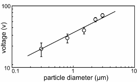
Figure 5: The voltage at which oscillation starts to occur, $V$, versus the particle diameter, $d$. Apparently $V$ increases with $d$, indicating higher voltage is needed for the oscillation of droplets coated with larger particles. The dependence is consistent with the solid line of $V\propto d^{0.5}$ predicted by our model.

Moreover, this analysis predicts a general trend for the oscillation of droplets coated by different sized particles. When the electrical stress balances the capillary pressure, $\epsilon_{0}\epsilon E_{loc}^{2}\sim(\gamma/L)$, oscillation should start to occur. Plugging in the typical conditions of $L\sim d$ and $E_{loc}\sim V/d$, we obtain $V\propto d^{0.5}$. Therefore, for droplets coated by larger particles, oscillation should start to occur at a larger voltage $V$. To test this prediction, we perform measurements with different particle sizes and vary $d$ by one order of magnitude. Indeed we observe the increase of $V$ with respect to $d$, which is consistent with the predicted relation $V\propto d^{0.5}$ (see Fig.5). This agreement provides another experimental evidence for our model.

In conclusion, we achieve the systematic coalescence of Pickering emulsion droplets by applying high enough electric field. The droplets coalesce via two distinct approaches: the normal and abnormal coalescence. During the normal coalescence, a liquid bridge grows continuously and merges two droplets together, similar to the liquid droplet coalescence but with a much slower speed. In the abnormal coalescence, however, completely different behaviors emerge: a liquid bridge forms but fails to grow indefinitely; instead it breaks up spontaneously due to the geometric constraint of particle shells. This connecting-then-breaking cycle repeats multiple times, until the defects grow large enough and establish a stable connection. In depth analysis indicates that when the defect size is much larger than the particle diameter, normal coalescence will show up; while the abnormal coalescence appears for smaller defects. Moreover, droplets coated by larger particles require higher voltages to oscillate and coalesce. This study generalizes the understanding of coalescence to a more complex system, and may find useful applications in the industries related to Pickering emulsions.

G. C., P. T. and L. X. are supported by Hong Kong RGC (CUHK404211, CUHK404912 and direct Grant 2060442). J. P. H. is supported by NNSFC (11075035/11222544), Fok Ying Tung Education Foundation (131008), and Shanghai Rising-Star Program (12QA1400200).

References

- (1) J. Thomson and H. Newall, Proc. R. Soc. London 39, 417 (1885).
- (2) L. Duchemin, J. Eggers, and C. Josserand, J. Fluid. Mech. 487, 167 (2003).
- (3) D. G. A. L. Aarts and H. N. W. Lekkerkerker, J. Fluid Mech. 606, 275 (2008).
- (4) S. C. Case and S. R. Nagel, Phys. Rev. Lett. 100, 084503 (2008).
- (5) S. C. Case, Phys. Rev. E 79, 026307 (2009).
- (6) J. D. Paulsen et al, PNAS 109, 6857 (2012).
- (7) D. G. A. L. Aarts et al, Phys. Rev. Lett. 95, 164503 (2005).
- (8) A. Menchaca-Rocha, A. Martínez-Daávalos, R. Núñez, S. Popinet, and S. Zaleski, Phys. Rev. E 63, 046309 (2001).
- (9) W. Ramsden, Proc. R. Soc. London 72, 156 (1903).
- (10) S. U. Pickering, J. Chem. Soc. 91, 2001 (1907).
- (11) O. D. Velev, A. M. Lenhoff, and E. W. Kaler, Science 287, 2240 (2000).
- (12) A. D. Dinsmore, M. F. Hsu, M. G. Nikolaides, M. Marquez, A. R. Bausch, and D. A. Weitz, Science 298, 1006 (2002).
- (13) D. Lee and D. A. Weitz, Adv. Mater. 20, 3498 (2008).
- (14) J. S. Eow, M. Ghadiri, A. O. Sharif, and T. J. Williams, Chem. Eng. J. (London) 84, 173 (2001).
- (15) S. Simovic, P. Heard, H. Hui, Y. Song, F. Peddie, A. K. Davey, A. Lewis, T. Rades, and C. A. Prestidge, Mol. Pharmaceutics 6, 861 (2009).
- (16) K. Ahn, J. Agresti, H. Chong, M. Marquez, and D. A. Weitz, Appl. Phys. Lett. 88, 264105 (2006).
- (17) A. B. Subramaniam, M. Abkarian, L. Mahadevan, and H. A. Stone, Nature 438, 930 (2005).
- (18) A. R. Studart, H. C. Shum, and D. A. Weitz, J. Phys. Chem. B 113, 3914 (2009).
- (19) E. J. Stancik, M. Kouhkan, and G. G. Fuller, Langmuir 20, 90 (2004).
- (20) H. Fan and A. Striolo, Soft Matter 8, 9533 (2012).
- (21) G. I. Taylor, Proc. R. Soc. A 280, 383 (1964).
- (22) H. A. Stone, J. R. Lister, and M. P. Brenner, Proc. R. Soc. A 455, 329 (1999).
- (23) R. T. Collins, J. J. Jones, M. T. Harris, and O. A. Basaran, Nature Physics 4, 149 (2008).
- (24) P. R. Brazier-Smith, S. G. Jennings and J. Latham, Proc. R. Soc. Lond. A 325, 363 (1971).
- (25) X. G. Zhang, O. A. Basaran, and R. M. Wham, AIChE J. 41, 1629 (1995).
- (26) W. D. Ristenpart, J. C. Bird, A. Belmonte, F. Dollar, and H. A. Stone, Nature (London) 461, 377 (2009).
- (27) J. C. Bird, W. D, Ristenpart, A. Belmonte, and H. A. Stone, Phys. Rev. Lett. 103, 164502 (2009).
- (28) W. T. M. Irvine, V. Vitelli and P. M. Chaikin, Nature 468, 947 (2010).
- (29) can be calculated as . Here is the relative permittivity of water, is the vacuum permittivity, and is the conductivity of our salt water. The detailed derivation of is the following: from charge conservation we have ; also from Gauss’s law we have . Combining the two gives: , with . This equation has the solution: , which gives the characteristic relaxation time .