Systematics in Metallicity Gradient Measurements I : Angular Resolution, Signal-to-Noise and Annuli Binning

Abstract

With the rapid progress in metallicity gradient studies at high-redshift, it is imperative that we thoroughly understand the systematics in these measurements. This work investigates how the [N ii] /H$\alpha$ ratio based metallicity gradients change with angular resolution, signal-to-noise (S/N), and annular binning parameters. Two approaches are used: 1. We downgrade the high angular resolution integral-field data of a gravitationally lensed galaxy and re-derive the metallicity gradients at different angular resolution; 2. We simulate high-redshift integral field spectroscopy (IFS) observations under different angular resolution and S/N conditions using a local galaxy with a known gradient. We find that the measured metallicity gradient changes systematically with angular resolution and annular binning. Seeing-limited observations produce significantly flatter gradients than higher angular resolution observations. There is a critical angular resolution limit beyond which the measured metallicity gradient is substantially different to the intrinsic gradient. This critical angular resolution depends on the intrinsic gradient of the galaxy and is $\leq 0.02^{\prime\prime}$ for our simulated galaxy. We show that seeing-limited high-redshift metallicity gradients are likely to be strongly affected by resolution-driven gradient flattening. Annular binning with a small number of annuli produces a more flattened gradient than the intrinsic gradient due to weak line smearing. For 3-annuli bins, a minimum S/N of $\sim 5$ on the [N ii] line is required for the faintest annulus to constrain the gradients with meaningful errors.

1. Introduction

The chemical abundance distribution within galaxies at local and high redshift offers unique insights into the formation and evolution of galaxies. Indeed, the first simple formation models of our Milky Way were built upon observational knowledge of the Galactic chemical distribution and stellar dynamics (Eggen et al., 1962; Searle & Zinn, 1978).

For local galaxies, the existence of radial metallicity gradients has been established in most spiral galaxies using abundances in H ii regions (Pagel & Edmunds, 1981; Edmunds & Pagel, 1984; Evans, 1986; Garnett & Shields, 1987; Vilchez et al., 1988; Shields, 1990; Vila-Costas & Edmunds, 1992; Zaritsky et al., 1994; Dutil & Roy, 1999). The radial metallicity gradients are negative, with a higher metallicity towards the galactic center. On the other hand, mergers and barred galaxies have shallower or flattened gradients due to interaction-induced gas flows or bar induced gas inflows (Kewley et al., 2010; Rupke et al., 2010a, b).

In the classic galactic chemical evolution models, the radial metallicity gradients formed during inside-out galaxy mass assembly. In this scenario, gas infall timescales increase with galactocentric distance (Prantzos & Boissier, 2000; Chiappini et al., 2001; Mollá & Díaz, 2005; Magrini et al., 2007; Fu et al., 2009). However, even among inside-out formation models, no consensus has been reached on the direction and magnitude of the cosmic time evolution of the metallicity gradient.

The time evolution of the metallicity gradient in disk galaxies provides tight constraints on the historical events that mark the galactic disc structure evolution. The cosmic metallicity gradient evolution is directly linked with the size-growth, external gas accretion, galactic-scale outflows, and any internal transportation of the star-forming gas in galaxies. Early analytical models such as Edmunds & Greenhow (1995) have provided perceptive predictions on how the gas flows can change the origin and evolution of the metallicity gradient. Current $\Lambda$CDM cosmological hydrodynamic simulations now incorporate the prescriptions for galactic chemical evolution models and initial predictions for the metallicity gradient evolution with redshift are beginning to emerge (e.g., Pilkington et al., 2012). To guide and compare with these models and simulations, it is of crucial importance to establish an observational baseline for the time evolution of metallicity gradients in galaxies.

Observational constraints on the time evolution of the metallicity gradient have been scarce and are traditionally based on indirect methods using different age-tracers such as Cepheids, planetary nebulae, and open clusters in the Milky Way (Andrievsky et al., 2002; Maciel et al., 2003; Maciel & Costa, 2010). Direct observations of metallicity gradients at high redshift have not been possible until the recent employment of high sensitivity near infrared (NIR) integral field spectrographs (IFS) on large telescopes.

As a result, it is only in the past three years that the first radial metallicity gradient measurements have been made for high-redshift galaxies (Jones et al., 2010; Cresci et al., 2010; Yuan et al., 2011; Queyrel et al., 2012; Swinbank et al., 2012; Jones et al., 2012). These integral field unit (IFU) studies can be divided into three categories according to their angular resolution: (1) gravitationally lensed galaxies with adaptive optics (AO) aided observations (Jones et al., 2010; Yuan et al., 2011; Jones et al., 2012); (2) non-lensed galaxies with AO aided observations (Swinbank et al., 2012); (3) non-lensed galaxies with seeing-limited observations (Cresci et al., 2010; Queyrel et al., 2012). It is interesting to note that the steepest gradients discovered so far are all observed in the highest resolution category (1), whereas much shallower gradients are reported in categories (2) and (3).

Compared to local observations, the most obvious restrictions at high redshift are angular resolution and signal-to-noise (S/N). Because of these impediments, simplifications in data analysis such as annular binning are used to gain S/N in spectra. It is unknown whether/how the observational limitations and data analysis techniques for high redshift studies cause systematic uncertainties in the measured metallicity gradients.

With the rapid progress in metallicity gradient observations at high redshift, it is imperative that we understand the systematics in our measurements before embarking on surveys of large samples.

This paper is the first of a series devoted to understanding the systematics of metallicity gradient measurements. Specifically, this paper investigates how the metallicity gradient is affected by the angular resolution, S/N, and annular binning that are characteristic for high-$z$ studies.

We use two approaches: 1. We downgrade the highest angular resolution and S/N IFU data from our published AO-aided lensed galaxy to lower resolutions and then recalculate the metallicity gradients at different resolutions; 2. We simulate the IFU data at high-$z$ using a local starburst galaxy with a known gradient. We then compare the metallicity gradients measured from the simulated data at different angular resolutions and S/N ratios. We find that the metallicity gradient changes systematically with angular resolution, S/N and the annular binning parameters.

This paper is organized as follows. In Section 2, we list the assumptions used. In Section 3 and Section 4, we describe our two approaches and results. We compare our results with literature data in Section 5. We discuss our explanations for the systematic uncertainties in Section 6. We present our conclusions and future directions in Section 7. Throughout this paper we use a standard $\Lambda$CDM cosmology with $H_{0}$= 70 km s^-1 Mpc^-1, $\Omega_{M}$=0.30, and $\Omega_{\Lambda}$=0.70.

2. Overall Assumptions

Many factors can affect metallicity gradient measurements. In order to analyze the role of angular resolution, S/N and annular binning parameter, it is necessary to decouple these effects from other factors that may affect the metallicity gradient. We hold all other parameters that may affect the gradient constant. To focus on the systematics of the angular resolution, S/N and annular binning on the metallicity gradient measurement, we find it necessary to impose the following assumptions and simplifications:

• We use the [N ii] /H$\alpha$ ratio as calibrated in Pettini & Pagel (2004) (the PP04N2 method hereafter) to calculate metallicity. Because of the relatively easy access, [N ii] /H$\alpha$ ratios will continue to be the most practical metallicity diagnostics for high-$z$ studies in the near future. In Kewley & Ellison (2008), we showed that the absolute abundance scale differs for different calibrations. However, relative metallicities, such as metallicity gradients are robust to within 0.03 dex on average. To avoid problems with the absolute abundance calibration scale, we only apply the single PP04N2 diagnostic. We have verified that the results for our local galaxy are unchanged when independent diagnostics such as the Kobulnicky & Kewley (2004) and McGaugh (1991) calibrations are applied.

• We assume that the metallicity gradient can be fitted by one linear function (c.f., Bresolin et al., 2009b). We express gradients in dex per kpc. We do not consider how the intrinsic sizes of galaxies may affect the metallicity gradient measurement (e.g., Jones et al., 2012).

• We assume that the metallicity distributions in disk galaxies have cylindrical symmetry, i.e., azimuthal abundance variations are not significant (e.g., Kennicutt & Garnett, 1996; Bresolin et al., 2009a).

• We assume the galactic center is well-defined and is aligned with the peak of H$\alpha$ emission. Locating the galactic center is straightforward for local galaxies, but may not be unambiguous for high-$z$ galaxies because of their irregular morphology (e.g., Abraham et al., 1996; Giavalisco et al., 1996). For similar reasons, we do not correct for the inclination angle of the galaxy as it is not well constrained for high-$z$ galaxies. Our aim is to simulate high-redshift data and to analyze that data under the same assumptions and limitations that affect high redshift galaxy observations.

• We only consider metallicity gradients for isolated disks.

• The inhomogeneity of metal distribution has been found in both the radial and vertical directions of the galactic discs, as well as in early-type galaxies. Although abundance gradients in the vertical direction and in early-type galaxies are equally important (Franx & Illingworth, 1990; Henry & Worthey, 1999; Marsakov & Borkova, 2006), we confine our discussion to the radial gas-phase metallicity in disk galaxies.

• The uncertainties stemming from lensing models and the effects of shocks and AGN (e.g., Wright et al., 2010; Rich et al., 2011; Yuan et al., 2012; Westmoquette et al., 2012) are beyond the scope of the paper and will be investigated in a future paper in this series.

Note that each of the above items may play an important role in metallicity gradient studies. We hold them constant in order to filter out the systematics of the angular resolution, S/N and annular binning on the metallicity gradient measurement. By comparing metallicity gradients obtained for the same data within the same galaxy using the same calibration, we avoid the effects of the issues highlighted above.

3. Methodology A: Downgrade High-Redshift High Angular Resolution Data

The highest intrinsic angular resolution achieved ($\sim 0.02^{\prime\prime}$) in metallicity gradient measurements at high-$z$ is in category (1): gravitationally lensed galaxies with adaptive optics (AO) (Jones et al., 2010; Yuan et al., 2011; Jones et al., 2012). Among these studies, the grand-design spiral Sp1149 at $z=1.49$ is most spectacular and suitable for detailed metallicity analysis because of its clear face-on morphology and fortuitously uniform lensing magnification (Yuan et al., 2011). Note that all high-$z$ observations of galaxies suffer from the loss of low surface brightness pixels. The magnification of gravitationally lensed galaxies helps to alleviate the problem by bringing more spatial elements with low surface brightness within the detection limit compared to non-lensed cases. We therefore use Sp1149 as our high redshift testing galaxy.

3.1. Integral field spectroscopy of Sp1149

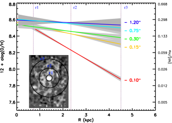
Figure 1.— Metallicity ([N ii] /H$\alpha$ ratio) vs. radius for Sp1149 downgraded to different angular resolution FWHM = 0.1, 0.15, 0.3, 0.75, and 1.2 arcsec (in different colors). The solid lines are the best-fit of the metallicity slope, the 1-$\sigma$ errors of the slope from linear regression are shown as shaded regions around the solid lines. The imbedded panel on the lower left shows the original OSIRIS H$\alpha$ map with the three annuli marked. The original data has an angular resolution of 0.1^′′ (FWHM), corresponding to the pixel scale of the data. Note that because of lensing magnification, the corresponding intrinsic angular resolution in this case is 0.02^′′.

Sp1149 was observed using the Laser Guide Star Adaptive Optics aided integral field spectrograph (OSIRIS; Larkin et al. 2006) on KECK II in 2011. We achieved an image-plane angular resolution of $0\farcs 1$, corresponding to a source-plane resolution of $\sim$ 0.02^′′ (170 pc). The pixel scale we use for Sp1149 is $0\farcs 1$, with a field of view (FOV) of 4.8^′′ by 6.4^′′ and a spectral resolution of $R\sim$3400.

Sp1149 is a rare lensing case as it is stretched almost equally by $\sim$ 5 times on each side of the two-dimensional image. As a result, the source-plane morphology looks almost identical to the image-plane morphology. The error on the lensing magnification of Sp1149 is $<10\%$ (Smith et al., 2009; Yuan et al., 2011).

In Yuan et al. (2011), we derive the metallicity gradient for Sp1149 by integrating the spectrum in three annuli corresponding to a physical length of r1$=$0.72$\pm$0.1 kpc, r2$=$2.34$\pm$0.2 kpc, r3$=$4.5$\pm$0.4 kpc. The choice of the annuli is such that the integrated spectra could reach S/N $>$ 5 for the weak [N ii] lines. The [N ii] line is robustly detected at S/N $>$ 5 for the inner two annuli and is a 3$\sigma$ detection for the outer annulus which we give an upper limit. In the next subsection, we use the same steps to derive metallicity gradients on the resolution-downgraded data of Sp1149.

3.2. Sp1149 Downgraded to Different Angular Resolutions

For each wavelength slice, we convolve the spatial pixels with a Gaussian kernel of a range of full width half maximum (FWHM) values (0.2^′′-0.8^′′). We then re-extract the spectra using the same three annuli as in Yuan et al. (2011). We use the same line-fitting procedures as used in Yuan et al. (2011): Gaussian profiles were fitted simultaneously to the three emission lines: [N ii]$\,\lambda$6548, 6583 and H$\alpha$. The line profile fitting was conducted using a $\chi^{2}$ minimization procedure which takes into account the greater noise level close to atmospheric OH emissions. The centroid and velocity width of [N ii]$\,\lambda\lambda$6548, 6583 lines were constrained by the velocity width of H$\alpha$$\,\lambda$6563, and the ratio of [N ii]$\,\lambda$6548 and [N ii]$\,\lambda$6583 is constrained to the theoretical value (Osterbrock, 1989). We fit the [N ii] /H$\alpha$ ratios in the three annuli and obtain the metallicities using the PP04N2 method (Pettini & Pagel, 2004). In Figure 1 we show the metallicity gradient and 1-$\sigma$ error of the fit to metallicity ([N ii] /H$\alpha$ ratio) vs. radius for the downgraded IFU data in a few cases of angular resolution FWHM.

We see from Figure 1 that the measured metallicity gradient flattens with poorer angular resolution FWHM. With an angular resolution FWHM above $\sim$0.75^′′, inverted (positive) gradients begin to appear within the errors of the linear fitting.

To determine whether the trend continues at even lower angular resolution, we downgrade the data using a range of angular resolution FWHM between the original 0.1^′′ resolution and a fiducially large 2.0^′′ resolution. We find that relation between the metallicity gradients and the angular resolution FWHM follows an interesting curve (Figure 2).

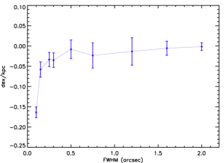
Figure 2.— The measured metallicity gradient and the 1-$\sigma$ error as a function of the FWHM angular resolution based on the data of Sp1149 at $z=1.49$ (Yuan et al., 2011). The smallest angular resolution corresponds to the actual observed resolution of 0.1^′′ or 0.02^′′ intrinsic resolution after correcting for lensing magnification.

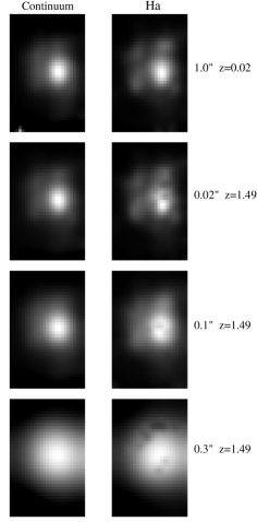
Figure 3.— The continuum and wavelength-collapsed H$\alpha$  image derived from the WiFeS data of Sp17222 (first row), and from the simulated Sp17222 at $z=1.49$ in different angular resolution FWHM (row 2-3: examples of FWHM  =  0.1^′′, 0.2^′′, 0.3^′′). We see that at FWHM $\geq$ 0.3^′′, the H$\alpha$ clumps on the outer disk of Sp17222 are not resolved anymore. The artifacts (black dots) on the simulated data are regions of low S/N ($<$ 5) on the H$\alpha$ line.

Figure 4.— Derived [N ii] /H$\alpha$ -based metallicity gradient for the local data of Sp17222. Left: H$\alpha$ intensity derived from the WiFeS datacube. We use the same three annuli as defined on the simulated high-$z$ data. The average spectra (zoomed in for the [N ii] and H$\alpha$  vicinity) in the three annuli are shown on the right panel (a1-a3). The flux is in unit of $10^{-16}$ ergs s^-1 cm${}^{-2}\AA^{-1}$. The panel on the bottom right shows the metallicity gradient derived using the three annuli (black) in comparison with a full sampling (red) without binning.

Figure 2 suggests that there is a critical angular resolution, below which the measured gradient is significantly more steepend. Above this critical resolution, e.g., under seeing-limited conditions, the gradient approaches a very shallow or nearly flat slope.

The behavior of the gradient vs. angular resolution is worrisome. Ideally, the measured gradient should not be a function of angular resolution within the observational errors. If a higher angular resolution more closely represents the real gradient, then what is the angular resolution required to recover the intrinsic gradient ? We address this question in Section 4.

4. Methodology B: Simulate High-Redshift IFU Observation Using Local Data

4.1. Local Spiral Galaxy IRAS F17222-5953 (Sp17222)

In order to simulate an IFS observation at high-$z$, we choose a local galaxy that has star formation concentrated at the galactic nucleus instead of in the spiral arms. We use the isolated luminous infrared galaxy IRAS F17222$-$5953 (Sp17222) at $z=0.021$. Sp17222 is relatively face-on, has a morphological type of Sbc, and a moderate SFR (H$\alpha$) of $\sim$11 M_⊙ yr^-1. The optical IFU data of Sp17222 is adopted from the Wide Field Spectrograph (WiFeS) Integral Field Unit (IFU) Great Observatory All-Sky LIRG Survey (GOALS) Sample (WIGS) (Rich et al., 2012).

Briefly, the IFU data were taken using WiFeS at the Mount Stromlo and Siding Spring Observatory (SSO) 2.3 m telescope (Dopita et al., 2010). The blue and red spectra of WiFeS were observed with a resolution of R3000 and R7000 and wavelength coverage of $\sim$3500-5800 $\AA$ and $\sim$ 5500-7000 $\AA$ respectively. We use the fully reduced and flux calibrated data from Rich et al. (2012). The pixel scale of WiFeS is 0.5^′′, with a field of view (FOV) of 25^′′$\times$38^′′. The reduced data are binned by 2 pixels in the spatial direction, yielding an effective spatial resolution of 1.0^′′$\times$1.0^′′.

4.2. Simulating IFU Observations of Sp17222 at $z=1.49$

To make realistic comparisons with observed IFU data, we fix Sp17222 at the redshift of Sp1149 ($z=1.49$). We derive the size and surface brightness distribution for each redshifted wavelength slice using basic equations of angular diameter distance and luminosity distance, and based on the conservation of total luminosity. Due to pure cosmology effects, the angular size and total flux of Sp17222 are reduced by $\sim 0.05$ and $\sim 2.9\times 10^{-5}$ respectively at $z=1.49$.

Because the angular size becomes smaller at higher redshift, an angular scale of 0.02^′′ is required to fully recover the spatial samplings of the local IFU data. We thus set the highest FWHM resolution of our simulation as 0.02^′′.

The original Poisson-noise dominated optical spectra are shifted into the NIR at $z=1.49$, and real NIR data are sky-background dominated. We compose a noise spectrum at the spectral resolution of WiFes by interpolating the sky-residuals of our OSIRIS datacube. The noise spectrum represents the sky OH emission residuals in a real observation in the NIR at $z=1.49$. The noise spectrum is scaled and added to the redshifted spectrum of each spaxel according to the required input S/N.

We define the input S/N of our simulation on the spaxel where H$\alpha$ emission peaks. For example, an input S/N of 100 means that the noise spectrum is scaled and added to the target spectrum such that the S/N ratio of the H$\alpha$ line on the brightest pixel is 100. To facilitate comparison with observations, we also measure the observed S/N of the [N ii] lines in outer annulus on the simulated datacube (Section 4.5).

Note that in this simulation, we do not consider any intrinsic evolutionary effect except that we multiply the total flux of the original IFU data by a factor of 20. The factor of 20 is adopted for two reasons: 1. The SFR of galaxies at $z\sim 2$ are found to be $\sim 20$ higher than galaxies at $z\sim 0$ at a fixed mass of $\sim 10^{10}~{}M{{}_{\odot}}$ (e.g., Noeske et al., 2007a, b; Zahid et al., 2012); 2. Without manually increasing the total flux, Sp17222 would have been under the detection limit of any current NIR IFU instrument. We find that by increasing the intrinsic flux by 20, Sp17222 would be well detected in NIR IFU spectrographs such as OSIRIS on KECK. The factor of $\sim$ 20 also coincides with the lensing flux magnification of Sp1149 in Section 3.

Finally, following similar steps as in Section 3, we convolve the spatial pixels with different angular resolution FWHM and generate a set of simulated IFU data at $z=1.49$.

For both the local and simulated datacube, we use the same line-fitting procedures as described in Yuan et al. (2011) and in Section 3.2. Figure 3 shows the continuum and H$\alpha$ emission line image derived from the original WiFeS data of Sp17222, and from the simulated high-$z$ Sp17222 datacube in different angular resolutions.

4.3. The Effect of Annular Binning on Metallicity Gradient

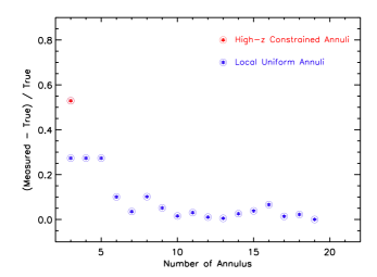
Figure 5.— The percentage of the difference between the measured metallicity gradient in annuli and the true metallicity gradient in full sampling as a function of the number of annulus used. The blue circles are the measurements from the annuli that are uniformly divided from the galactic center to the outer disk. The red circle shows the measurement from the 3 annuli that are defined on the high-z data constrained by the S/N of the weak [N ii] lines (Section 4.3).

Annular binning is a commonly used method to derive metallicity gradients for low S/N high-$z$ data (Jones et al., 2010; Yuan et al., 2011; Queyrel et al., 2012; Swinbank et al., 2012). In order to quantify the effect of annular binning on metallicity gradient measurements, we compare the effect of 3-annuli binning with full sampling without binning. Since only the local datacube has sufficient spatial resolution and S/N simultaneously to compare a full and 3-annuli sampling, we test these 2 types of samplings on the original datacube of Sp17222 first, without degrading the resolution.

We show the metallicity gradients derived from a 3-annuli binning and a full sampling in radius in the lower right panel of Figure 4. The three annuli are defined on the simulated high-$z$ data and they are chosen such that the [N ii] line from the outer-most annulus is robustly detected (S/N $\geq$ 5) on all annuli of the high-$z$ datacube, consistent with current high-z studies (Jones et al., 2010; Yuan et al., 2011).

We see from Figure 4 that the gradient from annular binning is shallower than the gradient derived from full samplings. In the case of Sp17222, binning in 3 annuli yields a metallicity gradient of -0.016$\pm$0.004 dex kpc^-1, whereas the fulling sampling yields -0.032$\pm$0.003 dex kpc^-1.

To further investigate the relation between the measured gradient and the number of annuli used, we calculate the measured metallicity on the local IFU data of Sp17222 using a range of annuli. Note that the annuli in Figure 4 are defined on the simulated high-$z$ data and are constrained by the S/N of the [N ii] line from the outer-most annulus. The choice of the annuli is therefore defined on the emission line flux distribution of the high-$z$ data. A more straight-forward method of defining annuli is to divide the radius equally into N uniform bins. These uniform annuli can be applied to the local data where the requirement of S/N$>5$ on the [N ii] line is not a constraint for most radii. We therefore divide the Sp17222 data equally in radius using a number of N_min = 3 and N_max = 20 annuli. We show in Figure 5 the percentage of the difference between the measured metallicity gradient from different numbers of annuli and the true metallicity gradient from full sampling as a function of the number of annuli. We find that with N=3-5 uniform annuli, the measured gradients are close to the true gradient within $\sim$ 30%; with N$\geq$6 uniform annuli, the true gradient can be recovered to within 10%. We also show that the metallicity gradient from the uniform 3-annuli is closer to the true gradient (28% c.f. 54%) than the S/N constrained 3-annuli employed on the high-z data.

In summary, we see that binning in 3 (or another small number of) annuli introduces non-negligible systematic errors on the metallicity gradient measurement. The definition of the location of the annuli also plays a non-negligible role in the metallicity gradient measurement. The choice of the annuli used in high-z studies is weighted by the S/N of the weak [N ii] lines and can only recover the true gradient to within 54% in the simulated case of Sp17222. The choice of uniformly distributed annuli recovers the true gradient significantly better. In the case of Sp17222, using N $>$ 6 annuli can recover the true gradient to within 10%.

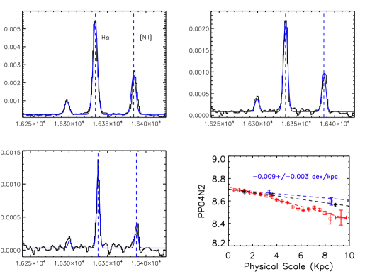
Figure 6.— Examples of the [N ii] and H$\alpha$ lines extracted from the 3 annuli on a simulated datacube (S/N=100, FWHM=0.02^′′). The panels are organized in the same order as in Figure 4, with the same flux and wavelength units. The panel on the bottom right shows the metallicity gradient (blue) based on the [N ii] and H$\alpha$  line ratios. The local 3-annuli (black) and full sampling (red) gradients are also shown for comparison.

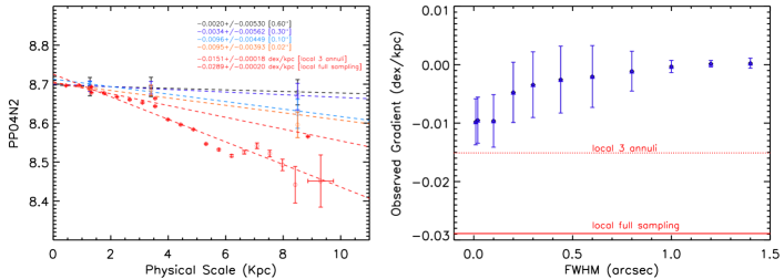
Figure 7.— Left: Metallicity vs. radius on the simulated datacube (S/N fixed at 100). Three-annuli bins are used. We show examples of a few angular resolution FWHM in different colors. For comparison, the three annuli and fully sampled metallicity of the local data are shown in red. Right: Simulated metallicity gradient as a function of angular resolution FWHM. The horizontal red lines show the location of the metallicity gradients measured on the local data using three annuli and full samplings respectively. We see that the local gradient is not recovered even in the highest resolution of the simulation (FWHM=0.02 ^′′).

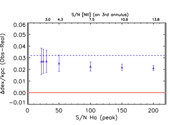
Figure 8.— The deviation of the measured gradient from the “true gradient” as a function of S/N (angular resolution fixed at 0.02^′′). The horizontal red line shows the true gradient measured on the fully sampled local data of Sp17222. The S/N marked on the bottom are defined on the peak spaxel of the H$\alpha$ emission line (Section 4.2). The corresponding S/N of the [N ii] line on the faintest annulus are marked on the top.

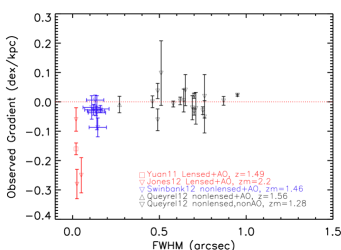
Figure 9.— The fact that measurements for different galaxies in different studies follow the same trend as Figure 2 and 7 strongly suggest that the angular resolution has played a role in causing the systematic difference in the metallicity gradient. The effect of angular resolution needs to be quantified before interpreting the metallicity gradient evolution with redshift.

4.4. The Effect of Angular Resolution on Metallicity Gradient Measurements

We extract the 3-annuli spectra for our simulated high-$z$ datacube with a range of angular resolution FWHM and S/N ratios. Figure 6 shows an example of the 3-annuli spectra and derived metallicity gradient. The example in Figure 6 has an angular resolution of FWHM=0.02^′′ and a limiting S/N of 100 on the H$\alpha$ line. A S/N of 100 on the H$\alpha$ line corresponds to a measured S/N of 7.5 on [N ii] line of the faintest annulus.

Figure 7 shows the PP04N2-based metallicity gradient for different angular resolution FWHM. We see the same trend in the simulated data as seen in Figure 1: the measured metallicity gradient is shallower as the FWHM increases. As the angular resolution FWHM approaches the seeing limited regime, the gradients are essentially consistent with a flat ($\sim$ 0) value. The curve of the metallicity gradients vs. the angular resolution FWHM relation is similar to Figure 2. However, the change of the FWHM from steep to shallow gradients is slower.

The deviation of the measured gradient from the true gradient measured from the fully sampled local data of Sp17222 can be derived from Figure 7. The closest gradient measurement we can obtain is $0.095\pm 0.004$ dex per kpc (true gradient = 0.032$\pm$0.004 dex per kpc), i.e., only 29% of the true gradient is recovered by the highest angular resolution and S/N observation simulated.

4.5. The Effect of S/N on Metallicity Gradient Measurements

Section 4.4 shows the high input S/N (100) case. As described in Section 4.2, the input S/N is defined on the H$\alpha$ line of the central pixel.

We repeat our analysis in Section 4.4 using a range of input S/N. We vary the S/N ratios as described in Section 4.2. We fix the angular resolution at FWHM=0.02^′′. Figure 8 shows the deviation of the measured gradient from the true gradient as function of S/N. The errors of the metallicity gradient are derived from the errors in the slope of the two-variable (metallicity and radius) linear regression. We see that the most significant effect of S/N is on the errors of the metallicity gradient measurement. The errors of the gradients decrease with S/N. At H$\alpha$ S/N (peak) $<$ 50 or [N ii] S/N (3^rd annulus) $<$5, the error bars of the gradient are so large that the gradients can not be meaningfully constrained, i.e., both a positive and negative gradient are consistent within the errors.

5. Metallicity Gradient vs. Angular Resolution from the Literature

As described in Section 1, current IFS studies on metallicity gradients can be divided into three categories according to their angular resolution: (1) gravitationally lensed galaxies with AO; (2) non-lensed galaxies with AO; (3) non-lensed galaxies under seeing-limited conditions. We gather the literature data in these 3 categories and examine the measured metallicity gradients with respect to the angular resolution FWHM used in the observations.

For category (1), we use the 5 lensed galaxies from Jones et al. (2010); Yuan et al. (2011); Jones et al. (2012). We exclude 1 merging system from the lensed galaxies because galaxy mergers are known to flatten metallicity gradients (Kewley et al., 2010; Rupke et al., 2010b; Rich et al., 2012). For (2), we use the 7 AO-corrected galaxies from Swinbank et al. (2012). The galaxy sample in Swinbank et al. (2012) is chosen from the High-Z Emission Line Survey (HiZELS) survey (Sobral, 2012) which targets H$\alpha$ emitters close to bright stars. For (3), we use the data of Queyrel et al. (2012), as 17 out of the 18 galaxies in Queyrel et al. (2012) are seeing-limited measurements, with 1 AO corrected measurement. The galaxy sample in Queyrel et al. (2012) is part of the MASSIV project (Contini et al., 2012) and is chosen based on the visibility of the H$\alpha$ line in J or H band. These 18 galaxies do not include interacting galaxies identified in Queyrel et al. (2012). Since [N ii] and H$\alpha$  lines are available for all the samples, we calculate the metallicities using the PP04N2 metallicity diagnostic. Note that the metallicity gradients in Queyrel et al. (2012) are based on the Pérez-Montero & Contini (2009) [N ii] /H$\alpha$ metallicity calibration, which we have converted to the PP04N2 metallicity calibration. The metallicity gradients are shown as a function of the angular resolution FWHM in Figure 9.

Note that there is a redshift difference among the three samples. The median redshift for sample (1) is $z\sim 2$, the median redshifts for samples (2) and (3) are $z\sim 1.5$ and $z\sim 1.3$ respectively. If the angular resolution effect does not play a role in these observations, one would be tempted conclude that the metallicity gradient is evolving from the steeper gradients at $z\sim 2$ to much shallower gradients at $z\sim 1$. However, relating Figure 9 with Figure 2 and Figure 7, we see a striking similarity in the behavior of the measured metallicity gradient vs. the angular resolution FWHM relation. The fact that the steepest gradients are only seen in the lensing+AO samples (including one galaxy at z$\sim$ 1.5) is consistent with our findings in the previous sections that there exists a critical angular resolution limit beyond which the absolute value of the gradients are significantly under-estimated. It is possible that angular resolution causes the trend in Figure 9. Until the effect of angular resolution on metallicity gradients is well understood, extreme caution must be taken when interpreting apparent evolution in metallicity gradients with redshift.

6. Discussion

6.1. Explanation of the angular resolution effect: “low S/N line smearing” effect

The PP04N2 based metallicity depends on the ratio of the [N ii]  and H$\alpha$ lines. The [N ii] lines are usually more than 3 times weaker than H$\alpha$ lines for normal star-forming regions. Given a negative radial metallicity gradient, much weaker [N ii]  lines are expected in the outer regions of a galaxy. Any spatial averaging/smoothing process selectively smears the low S/N [N ii]  line regions. As a result, the spatially averaged spectra are weighted more towards the regions of stronger [N ii]  lines, leading to over-estimation of the metallicity in the outer-disk. Accordingly, binning using small numbers of annuli has the same effect as lower resolution (i.e. larger angular resolution FWHM).

Using this argument, we would expect that the steeper the intrinsic gradient is, the larger the observed gradient is going to deviate from the intrinsic value. The curve of the gradient vs. FWHM relation (e.g., Figure 2, Figure 7, and Figure 9) would depend on the intrinsic shape of the metallicity gradient.

If low S/N line smearing is the cause of the angular resolution effect observed in Figure 2, Figure 7, and Figure 9, one would think that it is possible to cancel out the smearing effect by using a reversely weighted function. However, it is not straightforward to establish this anti-weighting function, as it relies on knowing the intrinsic gradient a priori. Moreover, if the “smearing” process is done by the atmosphere, it is impossible to de-convolve the observed FWHM back to the pre-smeared values, as it would be equivalent to finding an algorithm to “recover” the data with any wished angular resolution.

7. Conclusion

In this paper, we have demonstrated that the angular resolution, S/N and annular binning introduce significant systematic errors in metallicity gradient measurements at high-$z$.

We find that:

• The measured metallicity gradient changes systematically with angular resolution FWHM. Seeing-limited observations are likely to produce more flattened gradients than AO-aided high-resolution studies.

• There is a critical angular resolution FWHM range beyond which the measured metallicity is significantly more flattened than the intrinsic metallicity. This critical FWHM depends on the intrinsic gradient of the galaxy. For the two cases used in this work, the critical FWHM is $<0.02^{\prime\prime}$, only currently reachable with AO + gravitational lensing.

• For a fixed angular resolution, the errors of the metallicity gradient increase as S/N decrease. At low S/N ($<5$ for [N ii] line in the simulated case), the errors are so large that the gradient can not be meaningfully constrained.

• Three-annuli binning or any limited number of annular binning yields a more flattened gradient than the intrinsic gradient.

Until these effects are thoroughly understood, we urge caution in interpreting metallicity gradient evolution with redshift. Our next work is to build an empirical angular resolution library by simulating a large sample of high-z galaxies using local galaxies with known gradients.

References

- Abraham et al. (1996) Abraham, R. G., Tanvir, N. R., Santiago, B. X., Ellis, R. S., Glazebrook, K., & van den Bergh, S. 1996, MNRAS, 279, L47
- Andrievsky et al. (2002) Andrievsky, S. M., Bersier, D., Kovtyukh, V. V., Luck, R. E., Maciel, W. J., Lépine, J. R. D., & Beletsky, Y. V. 2002, A&A, 384, 140
- Bresolin et al. (2009a) Bresolin, F., Gieren, W., Kudritzki, R., Pietrzyński, G., Urbaneja, M. A., & Carraro, G. 2009a, ApJ, 700, 309
- Bresolin et al. (2009b) Bresolin, F., Ryan-Weber, E., Kennicutt, R. C., & Goddard, Q. 2009b, ApJ, 695, 580
- Chiappini et al. (2001) Chiappini, C., Matteucci, F., & Romano, D. 2001, ApJ, 554, 1044
- Contini et al. (2012) Contini, T., et al. 2012, A&A, 539, A91
- Cresci et al. (2010) Cresci, G., Mannucci, F., Maiolino, R., Marconi, A., Gnerucci, A., & Magrini, L. 2010, Nature, 467, 811
- Dopita et al. (2010) Dopita, M., et al. 2010, Ap&SS, 327, 245
- Dutil & Roy (1999) Dutil, Y., & Roy, J.-R. 1999, ApJ, 516, 62
- Edmunds & Greenhow (1995) Edmunds, M. G., & Greenhow, R. M. 1995, MNRAS, 272, 241
- Edmunds & Pagel (1984) Edmunds, M. G., & Pagel, B. E. J. 1984, MNRAS, 211, 507
- Eggen et al. (1962) Eggen, O. J., Lynden-Bell, D., & Sandage, A. R. 1962, ApJ, 136, 748
- Evans (1986) Evans, I. N. 1986, ApJ, 309, 544
- Franx & Illingworth (1990) Franx, M., & Illingworth, G. 1990, ApJ, 359, L41
- Fu et al. (2009) Fu, J., Hou, J. L., Yin, J., & Chang, R. X. 2009, ApJ, 696, 668
- Garnett & Shields (1987) Garnett, D. R., & Shields, G. A. 1987, ApJ, 317, 82
- Giavalisco et al. (1996) Giavalisco, M., Livio, M., Bohlin, R. C., Macchetto, F. D., & Stecher, T. P. 1996, AJ, 112, 369
- Henry & Worthey (1999) Henry, R. B. C., & Worthey, G. 1999, PASP, 111, 919
- Jones et al. (2010) Jones, T., Ellis, R., Jullo, E., & Richard, J. 2010, ApJ, 725, L176
- Jones et al. (2012) Jones, T., Ellis, R. S., Richard, J., & Jullo, E. 2012, ArXiv e-prints
- Kennicutt & Garnett (1996) Kennicutt, Jr., R. C., & Garnett, D. R. 1996, ApJ, 456, 504
- Kewley & Ellison (2008) Kewley, L. J., & Ellison, S. L. 2008, ApJ, 681, 1183
- Kewley et al. (2010) Kewley, L. J., Rupke, D., Zahid, H. J., Geller, M. J., & Barton, E. J. 2010, ApJ, 721, L48
- Kobulnicky & Kewley (2004) Kobulnicky, H. A., & Kewley, L. J. 2004, ApJ, 617, 240
- Larkin et al. (2006) Larkin, J., et al. 2006, New Astronomy Reviews, 50, 362
- Maciel & Costa (2010) Maciel, W. J., & Costa, R. D. D. 2010, in IAU Symposium, Vol. 265, IAU Symposium, ed. K. Cunha, M. Spite, & B. Barbuy, 317–324
- Maciel et al. (2003) Maciel, W. J., Costa, R. D. D., & Uchida, M. M. M. 2003, A&A, 397, 667
- Magrini et al. (2007) Magrini, L., Corbelli, E., & Galli, D. 2007, A&A, 470, 843
- Marsakov & Borkova (2006) Marsakov, V. A., & Borkova, T. V. 2006, Astronomy Letters, 32, 376
- McGaugh (1991) McGaugh, S. S. 1991, ApJ, 380, 140
- Mollá & Díaz (2005) Mollá, M., & Díaz, A. I. 2005, MNRAS, 358, 521
- Noeske et al. (2007a) Noeske, K. G., et al. 2007a, ApJ, 660, L47
- Noeske et al. (2007b) —. 2007b, ApJ, 660, L43
- Osterbrock (1989) Osterbrock, D. E. 1989, Astrophysics of gaseous nebulae and active galactic nuclei (Research supported by the University of California, John Simon Guggenheim Memorial Foundation, University of Minnesota, et al. Mill Valley, CA, University Science Books, 1989, 422 p.)
- Pagel & Edmunds (1981) Pagel, B. E. J., & Edmunds, M. G. 1981, ARA&A, 19, 77
- Pérez-Montero & Contini (2009) Pérez-Montero, E., & Contini, T. 2009, MNRAS, 398, 949
- Pettini & Pagel (2004) Pettini, M., & Pagel, B. E. J. 2004, MNRAS, 348, L59
- Pilkington et al. (2012) Pilkington, K., et al. 2012, A&A, 540, A56
- Prantzos & Boissier (2000) Prantzos, N., & Boissier, S. 2000, MNRAS, 313, 338
- Queyrel et al. (2012) Queyrel, J., et al. 2012, A&A, 539, A93
- Rich et al. (2011) Rich, J. A., Kewley, L. J., & Dopita, M. A. 2011, ApJ, 734, 87
- Rich et al. (2012) Rich, J. A., Torrey, P., Kewley, L. J., Dopita, M. A., & Rupke, D. S. N. 2012, ApJ, 753, 5
- Rupke et al. (2010a) Rupke, D. S. N., Kewley, L. J., & Barnes, J. E. 2010a, ApJ, 710, L156
- Rupke et al. (2010b) Rupke, D. S. N., Kewley, L. J., & Chien, L. 2010b, ApJ, 723, 1255
- Searle & Zinn (1978) Searle, L., & Zinn, R. 1978, ApJ, 225, 357
- Shields (1990) Shields, G. A. 1990, ARA&A, 28, 525
- Smith et al. (2009) Smith, G. P., et al. 2009, ApJ, 707, L163
- Sobral (2012) Sobral, D. 2012, in IAC Talks, Astronomy and Astrophysics Seminars from the Instituto de Astrofísica de Canarias, 291
- Swinbank et al. (2012) Swinbank, M., Sobral, D., Smail, I., Geach, J., Best, P., McCarthy, I., Crain, R., & Theuns, T. 2012, ArXiv e-prints
- Vila-Costas & Edmunds (1992) Vila-Costas, M. B., & Edmunds, M. G. 1992, MNRAS, 259, 121
- Vilchez et al. (1988) Vilchez, J. M., Pagel, B. E. J., Diaz, A. I., Terlevich, E., & Edmunds, M. G. 1988, MNRAS, 235, 633
- Westmoquette et al. (2012) Westmoquette, M. S., Clements, D. L., Bendo, G. J., & Khan, S. A. 2012, MNRAS, 424, 416
- Wright et al. (2010) Wright, S. A., Larkin, J. E., Graham, J. R., & Ma, C. 2010, ApJ, 711, 1291
- Yuan et al. (2012) Yuan, T.-T., Kewley, L. J., Swinbank, A. M., & Richard, J. 2012, ApJ, 759, 66
- Yuan et al. (2011) Yuan, T.-T., Kewley, L. J., Swinbank, A. M., Richard, J., & Livermore, R. C. 2011, ApJ, 732, L14+
- Zahid et al. (2012) Zahid, H. J., Dima, G. I., Kewley, L. J., Erb, D. K., & Davé, R. 2012, ApJ, 757, 54
- Zaritsky et al. (1994) Zaritsky, D., Kennicutt, Jr., R. C., & Huchra, J. P. 1994, ApJ, 420, 87