Self regulated shocks in massive star binary systems

Abstract

In an early-type, massive star binary system, X-ray bright shocks result from the powerful collision of stellar winds driven by radiation pressure on spectral line transitions. We examine the influence of the X-rays from the wind-wind collision shocks on the radiative driving of the stellar winds using steady state models that include a parameterized line force with X-ray ionization dependence. Our primary result is that X-ray radiation from the shocks inhibits wind acceleration and can lead to a lower pre-shock velocity, and a correspondingly lower shocked plasma temperature, yet the intrinsic X-ray luminosity of the shocks, $L_{\rm X}$ remains largely unaltered, with the exception of a modest increase at small binary separations. Due to the feedback loop between the ionizing X-rays from the shocks and the wind-driving, we term this scenario as self regulated shocks. This effect is found to greatly increase the range of binary separations at which a wind-photosphere collision is likely to occur in systems where the momenta of the two winds are significantly different. Furthermore, the excessive levels of X-ray ionization close to the shocks completely suppresses the line force, and we suggest that this may render radiative braking less effective. Comparisons of model results against observations reveals reasonable agreement in terms of $\log(L_{\rm X}/L_{\rm bol})$. The inclusion of self regulated shocks improves the match for $kT$ values in roughly equal wind momenta systems, but there is a systematic offset for systems with unequal wind momenta (if considered to be a wind-photosphere collision).

1. Introduction

A large fraction of massive stars reside in binary systems, with recent estimates of binarity for O-type stars of $\mathrel{\hbox to0.0pt{\lower 3.0pt\hbox{$\sim$}\hss}\raise 2.0pt\hbox{$>$}}70\%$ (Chini et al. 2012; Sana et al. 2012). In such systems, which consist of two hot luminous massive stars, the collision of the powerful stellar winds leads to the formation of high Mach number shocks that emit at X-ray wavelengths (Stevens et al. 1992). Historically, colliding winds binary (CWB) systems have been characterized by high plasma temperatures and an X-ray over-luminosity (compared to their expected single star brightness) (Pollock 1987; Chlebowski & Garmany 1991) with observational inferences corroborated by theoretical models (Luo et al. 1990; Stevens et al. 1992; Pittard & Stevens 1997). However, more recent studies examining a wider population and using the XMM-Newton and Chandra satellites indicate that short period WR+O and O+O-star binary systems have a ratio of $\log(L_{\rm X}/L_{\rm bol})\simeq-7$, similar to that expected for single O-stars (Owocki & Cohen 1999; De Becker et al. 2004; Oskinova 2005; Sana et al. 2006; Antokhin et al. 2008; Nazé 2009; Nazé et al. 2011; Gagné et al. 2011; Gagne et al. 2012). Therefore, superlative X-ray brightness - $\log(L_{\rm X}/L_{\rm bol})$ as high as -5 - appears to be reserved for the more massive CWBs with high mass-loss rates (e.g. WR25 - Raassen et al. 2003, Pollock & Corcoran 2006; WR140 - Pollock et al. 2005; $\eta$ Carinae - Corcoran 2005, Corcoran et al. 2010).

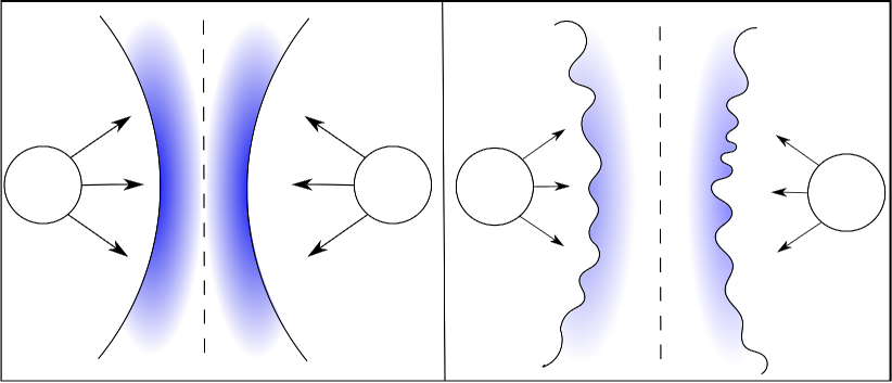
Figure 1.— Cartoon illustration depicting the wind-wind collision in an equal winds massive star binary system without (left) and with self regulating shocks (right). The stars are represented by the circles. Arrows indicate the wind direction, and arrow length indicates velocity magnitude. The solid and dashed lines demark the regions of post-shock stellar wind and the contact discontinuity, respectively. The shaded region indicates plasma temperature - fainter shading corresponds to lower temperature.

Can current models of CWBs account for the observed spread of over three orders of magnitude in X-ray luminosity from CWBs (Gagne et al. 2012)? Specific studies of archetypal systems around the higher luminosity end of the distribution have yielded promising results. For example, three dimensional simulations of $\eta$ Carinae and WR140, which include orbital motion, radiative cooling, and in some cases radiative driving, are able to explain the X-ray lightcurves and spectra reasonably well (Okazaki et al. 2008; Parkin et al. 2009, 2011; Russell et al. 2011). In contrast, models of WR22 by Parkin & Gosset (2011) over-predict $L_{\rm X}$ by up to two orders of magnitude, with the best agreement (a factor of roughly six over-estimate) achieved when a wind-photosphere collision occurs and the majority of the X-ray emission is extinguished. Problems also arise for lower mass CWB systems. A model of an O6V+O6V binary by Pittard (2009) and Pittard & Parkin (2010) revealed an estimated $\log(L_{\rm X}/L_{\rm bol})$ of between -6 and -6.3 (depending on the viewing angle). This should be compared against observed values for systems with orbital periods of 2-3 days that have $\log(L_{\rm X}/L_{\rm bol})$ between -6.2 and -7.3 (Nazé 2009; Gagné et al. 2011; Gagne et al. 2012). Pittard & Parkin (2010) have presented evidence that this discrepancy may, in part, be due to the spectral fitting procedure used to extract parameters from observations, which they show to under-predict the actual X-ray luminosity (which is known from the models) by up to a factor of two, particularly for short period systems where occultation may occur. Alternatively, the inconsistency with observations may indicate that some additional physics is required in the models.

Consideration of radiative wind driving in a massive star binary system led to the discovery of two interesting effects: radiative inhibition (Stevens & Pollock 1994) and sudden radiative braking (Owocki & Gayley 1995; Gayley et al. 1997). In the former, the acceleration of the stellar wind may be reduced by the radiation field of the binary companion, whereas the latter effect concerns hypersonic flows being effectively halted in their tracks enabling a wind-wind collision in systems where one would not occur on the basis of a ram pressure balance alone. One factor that has not been previously studied in the CWB paradigm is the influence of the ionizing X-rays from the wind-wind collision shocks on the wind driving. Stevens & Kallman (1990) examined the dependence of the radiative line force on X-ray ionization for the case of a high-mass X-ray binary system, finding that the stellar wind acceleration could be significantly suppressed by a particularly bright compact object because the excessive X-ray ionization reduces the radiative line force (see also Stevens 1991). This effect has also been explored for line-driven instability shocks embedded in a massive star’s wind (Krtička & Kubát 2009; Krtička et al. 2009) and for radiatively driven disk winds of active galactic nuclei (Proga et al. 2000).

In this paper we make the first attempt to examine the feedback of ionizing X-rays from the wind-wind collision shocks on wind acceleration in a massive star binary system. Because of the direct coupling between the radiation force that drives the stellar winds and the ionizing X-ray emission that results from the wind-wind collision, we term this effect self regulated shocks (SRSs). Fig. 1 depicts the basic scenario under consideration and highlights some key effects due to SRSs. Firstly, wind velocities are reduced (shorter arrows in the right panel) which causes a lower post-shock plasma temperature (fainter shading). Consequently, radiative cooling may become sufficiently important to introduce instabilities which will perturb the shock fronts (Stevens et al. 1992; Parkin & Pittard 2010; van Marle et al. 2011; Parkin et al. 2011; Lamberts et al. 2011). The goal of this work is to provide a qualitative picture, and initial quantitative estimates, of when/if the SRS effect might be important. Therefore, we will make simplifications in order to elucidate the physics.

The structure of this paper is as follows: In § 2 we calculate the influence of X-ray ionization on the line force due to an ensemble of spectral lines. The semi-analytical wind acceleration model is described in § 3, followed by results for model binary systems in § 4. An approximate model for SRSs is presented in § 5. We compare results to observations in § 6 and then discuss some implications of our findings, and possible avenues for going beyond the illustrative wind acceleration model adopted in this work, in § 7. The main conclusions of this work are summarised in § 8.

2. The line force

For the wind models that will be presented in § 3, we need to compute the radiation force due to spectral lines for appropriate stellar parameters while accounting for the influence of X-ray irradiation arising from a wind collision. We will adopt an approximate treatment of the radiation force due to spectral lines following Castor, Abbott, & Klein (1975) (hereafter CAK ) and closely follow the approach by Stevens & Kallman (1990) to estimate the effect of X-ray ionization on the line force – essentially, our goal is to repeat their calculations for the stellar parameters appropriate to our study. In this section we outline the method and the implementation used here. For full details of the methodology and discussions of its validity, we refer the reader to CAK , Abbott (1982) and Stevens & Kallman (1990).

The total force due to lines is given by,

$$f_{\rm rad}=\frac{\sigma_{\rm e}F}{c}M(t)\;,$$ (1)

where $\sigma_{\rm e}$ is the electron scattering opacity and $F$ is the radiative flux. $M(t)$ is known as the line force multiplier, which depends on the dimensionless optical depth parameter in a stellar wind, defined by

$$t=\sigma_{\rm e}\rho v_{\rm th}\left(\frac{dv}{dr}\right)^{-1}\;,$$ (2)

where $\rho$ is the mass density, $v_{\rm th}$ is the thermal velocity of a hydrogen atom and ${dv}/{dr}$ is the radial velocity gradient. The Sobolev optical depth of a spectral line between lower state $l$ and upper state $u$ is given by $\tau^{S}_{u,l}=\eta_{u,l}t$ where

$$\eta_{u,l}=\frac{hc}{4\pi}\frac{n_{l}B_{l,u}-n_{u}B_{u,l}}{\sigma_{\rm e}\rho v_{\rm th}}\;.$$ (3)

Here, $n_{l}$ and $n_{u}$ are the lower and upper level population number densities and $B_{l,u}$ and $B_{u,l}$ are the usual Einstein coefficients for absorption and stimulated emission, respectively. The force multiplier, $M(t)$, is composed from a sum over all line transitions

$$M(t)=\sum_{\rm lines}\Delta\nu_{D}\frac{F_{\nu}}{F}\frac{1-\exp(-\eta_{u,l}t)}{t}\;,$$ (4)

where $\Delta\nu_{D}$ is the Doppler width and $F_{\nu}$ is the specific flux at the line frequency ($\nu$).

To evaluate $M(t)$, we need to supply a list of line transitions (frequencies and oscillator strengths), specify the form of the radiation field $F_{\nu}$, and compute the associated level populations ($n_{l}$, $n_{u}$, relative to the total density $\rho$).

The line list used in this study is drawn from two sources. For low-ionization metal atoms/ions, we use the CD23 line database of Kurucz & Bell (1995). From this source we include elements with atomic number $6\leq Z\leq 30$ and include ionization stages i – v with the following exceptions: for C, we include only i – iv while for $Z>20$ we include ions i – vii, where available. In order to extend our calculations to regimes of higher ionization, we also included data from the chianti atomic database (Dere et al. 1997, 2009). From this source, we take line lists for H and He and the high ions of the astrophysically abundance metals: C, N, O, Ne, Mg, Si, S, Ar, Ca, Fe and Ni (for each of these metal, we include chianti line lists for all available ions that we did not take from Kurucz & Bell 1995; we excluded theoretically predicted lines from the database). In total, our line list contains $\sim 7.7\times 10^{5}$ transitions.

The stellar radiation field, $F_{\nu}$ was taken from ATLAS9 model atmosphere grids (Castelli & Kurucz 2004). For the specific stellar parameters used, see below.

The level populations ($n_{l}$, $n_{u}$) for each transition were computed in a two stage process. First we used Cloudy v10.00 (Ferland et al. 1998) to compute the ionization stage of a shell of gas illuminated by a specified radiation field. In all cases, we assumed that the irradiating spectrum contains two components: emission from the star and hard radiation associated with emission from the wind collision region. The shape of the stellar component was taken from the same model atmospheres used for $F_{\nu}/F$. In setting the intensity of this component, we follow Stevens & Kallman (1990) and consider only a single value for the ratio of the electron number density to the geometrical dilution factor ($n_{e}/W=3.5\times 10^{10}$ cm^-3). To describe the spectral shape of the hard ionizing radiation, we adopt a thermal Bremsstrahlung spectrum at a temperature of 10 keV. The intensity of this component is specified as an ionization parameter,

$$\xi=\frac{4\pi F_{\rm X}\mu m_{\rm H}}{\rho}$$ (5)

where, in this work, $F_{\rm X}$ is the flux of X-rays from the wind collision shocks, and $\rho$ is the gas density. The value of $\xi$ is varied to quantify the affect of X-ray ionization on $M(t)$. From the ion populations provided by the Cloudy calculations, we compute level populations assuming local thermodynamic equilibrium (LTE, adopting the gas temperature calculated by Cloudy). Although simplistic, this assumption makes it easy to compute the force multiplier reasonably quickly. Ideally, full non-LTE calculations should be performed for complete atomic models associated with each ion. This, however, would significantly complicate the calculation and is not expected to qualitatively affect our findings (see Stevens & Kallman 1990, for further discussion).

2.1. Example calculation

Using the procedure outlined above, we can calculate $M(t)$ accounting for the effects of excess ionization (as controlled by $\xi$). As an example, we show results for a star with effective temperature $T_{\rm eff}=38500$ K, surface gravity $\log g=3.92$ and solar metallicity $\log(Z/Z_{\odot})=0$ in Fig. 2.

Figure 2.— Force multiplier versus dimensionless optical depth parameter ($t$) for $\log\xi=$ -2, 0, 2 and 4 (solid lines). Dashed lines show our fits (see text). These calculations are for a star with $T_{\rm eff}=38500$ K, $\log g=3.92$ and $\log(Z/Z_{\odot})=0$. For comparison, we also show calculations from Abbott (1982) for a star with $T_{\rm eff}=40000$ K and $\log g=4.0$ (black spots).

As expected, our results are in good agreement with Stevens & Kallman (1990). For each value of $\xi$, $M$ is largest (and constant) when $t$ is sufficiently small that all lines are optically thin. At large $t$, $M$ decreases as lines become optically thick and saturate. For calculations with low ionization parameter ($\log\xi<0$), $M$ remains significant ($M\mathrel{\hbox to0.0pt{\lower 3.0pt\hbox{$\sim$}\hss}\raise 2.0pt\hbox{$>$}}1$) up to around $t\sim 1$ ($M$ is essentially independent of ionization parameter for $\log\xi<-2$). As found by Stevens & Kallman (1990), we also see that as $\log\xi$ is increased beyond zero, $M$ drops and the regime in which $M(t)$ is well-described by the optically thin limit extends to higher $t$-values. For $\log\xi>3$, the force multiplier is always small.

For comparison, we also show in Fig. 2 the $M$-values reported by Abbott (1982) from calculations for a star with similar parameters ($T_{\rm eff}=40000$ K, $\log g=4.00$ and $n_{e}/W=1.8\times 10^{11}$ cm^-3). Since no excess ionization radiation was included by Abbott (1982), his calculations should be compared to our results for the lowest ionization parameter shown ($\log\xi=-2$). In general, the agreement is very good – the biggest discrepancy occurs around $\log t=-2.5$ and is at worst a factor of two.

2.2. Parameterizing the force multiplier

Although the force multiplier $M$ can be directly used to specify the line force, it is convenient to parametrize its dependence on $t$ for use in wind calculations. Although this approach means that the full complexity of $M(t)$ is not captured, it is widely used because of the relative ease of manipulating simply-parametrized forms for $M(t)$ when deriving wind solutions.

The basic ansatz under the CAK approximation is to fit a power-law to the run of $M(t)$ with $t$,

$$M(t)=kt^{-\alpha}$$ (6)

where $\alpha$ defines the slope and $k$ the amplitude of $M$ at $t=1$ (i.e., $k=M(1)$). To capture the flattening of $M(t)$ for small $t$, we follow Owocki et al. (1988), and modify Eq (6) such that the force multiplier becomes constant at low $t$ (as it must in the optically thin limit),

$$M(t,\xi)=k(\xi)t^{-\alpha}\left[\frac{(1+\tau_{\rm max})^{1-\alpha}-1}{\tau_{\rm max}^{1-\alpha}}\right]$$ (7)

where $\tau_{\rm max}=\eta_{\rm max}(\xi)t$. In Eq (7) we now explicitly indicate that $M$ depends on both $t$ and $\xi$. Throughout this paper, we will choose to describe the influence of $\xi$ on $M$ via the CAK parameters $k(\xi)$ and $\eta_{\rm max}(\xi)$. Allowing for $\xi$-dependence in these quantities captures the two systematic changes in $M(t,\xi)$ with $\xi$: decreasing $\eta_{\rm max}(\xi)$ with increasing $\xi$ allows the turnover in $M(t)$ to shift to higher $t$ with increasing $\xi$, while a reduction in $k(\xi)$ at large $\xi$ describes the overall decrease in $M$ for larger ionization parameters.

We follow Stevens & Kallman (1990) in choosing that $\alpha$ does not vary with $\xi$. Although it is certainly possible to allow $\alpha$ to vary, this mostly just adds unwarranted complexity to the parametrization. As is clear from Fig. 2, the slope of $\log M$ versus $\log t$ is not constant, meaning that a best-fit $\alpha$ is in any case a function of the range across which it is fit. Therefore, in all of our calculations, we do not fit $\alpha$ but rather fix it to the value that is required in order to reproduce the correct observed terminal velocity for a single star of the appropriate spectral type in a standard CAK theory. For the example star discussed in Section 2.1, this is $\alpha=0.57$.

With $\alpha$ fixed, we derive values of $k(\xi)$ and $\eta_{\rm max}(\xi)$ by fitting our computed $M(t)$ curves to the functional form given by Eq (7). We restrict this fitting to $\log t<0$, the regime in which $M(t)$ is expected to be dynamically significant. To illustrate the accuracy of this approach, the derived fits from our example calculation are over-plotted in Fig. 2. As expected, the fits are always very good in the optically thin limit and generally agree to within a few tens of per cent across the range of interest (i.e. when $M\mathrel{\hbox to0.0pt{\lower 3.0pt\hbox{$\sim$}\hss}\raise 2.0pt\hbox{$>$}}1$). However, there are clear imperfections, particularly in cases where the slope of $M(t)$ deviates from a constant power law (e.g. in our $\log\xi=2$ case). Nevertheless, the parametrized form provides a convenient description and reproduces the force multiplier to within a factor of two, which is adequate precision for the purpose of this investigation. We provide tabulated values of $k(\xi)$ and $\eta_{\rm max}(\xi)$ in the Appendix.

2.3. Rescaling of the force multiplier

As mentioned in the previous section, in fitting $k(\xi)$ and $\eta_{\rm max}(\xi)$ we specified the value of $\alpha$ a priori with the aim that the resulting $M(t,\xi)$ produced a terminal wind velocity in agreement with observed values. We now also rescale the force multiplier $M(t,\xi)$ to produce a wind mass-loss rate in agreement with observed values, which equates to multiplying $k(\xi)$ by a correction factor. At the cost of some subjective rescaling, this approach has the advantage of ensuring that the line force used in the colliding-winds model in the following section will produce sensible wind parameters while also allowing the influence of X-ray irradiation to be explored. We note that this modification is of smaller magnitude than the current uncertainties in mass-loss rates and wind acceleration in massive stars (see Puls et al. 2008, for a recent review).

2.4. Results of the line force calculation

Line force calculations were performed for two massive stars: O6V and O4III (see Table 1 for full sets of stellar parameters). In Fig. 3 we show the resulting $k(\xi)$ and $\eta_{\rm max}(\xi)$. Clearly, for $\log(\xi)>0$ the line force is effectively suppressed, whereas for $\log(\xi)<0$ ionization effects are negligible and radiative acceleration is largely unaffected.

Figure 3.— Plots of the line force parameters $k$ (upper) and $\log(\eta_{\rm max})$ (lower) as a function of ionization parameter, $\xi$.

Table 1Parameters used for stellar model atmospheres

Model	$T_{\rm eff}$	$M_{\ast}$	$R_{\ast}$	$\log(L/L_{\odot})$	$\log(g)$	$Z$	$\dot{M}$	$v_{\infty}$	$k(\xi=0)$	$\alpha$
	$(K)$	$(M_{\odot})$	$(R_{\odot})$				(${\rm\hbox{${\rm\thinspace M_{\odot}}$}{\rm\thinspace yr}^{-1}\,}$)	(${\rm{\rm\thinspace km}{\rm\thinspace s}^{-1}\,}$)
O6V	38500	31.7	10.2	5.3	3.92	1	$2\times 10^{-7}$	2530	0.12	0.57
O4III	41500	48.8	15.8	5.8	3.73	1	$5\times 10^{-6}$	2750	0.18	0.63

3. The wind model

3.1. Radiatively driven winds

To compute the wind acceleration we follow Stevens et al. (1992). Alterations have been made to couple the model with a means of estimating the X-ray luminosity from the wind-wind collision shocks, and then allow for an ionization parameter ($\xi$) dependence of the line force. The calculation proceeds by solving for the wind of one of the stars, with the influence of the companion star appearing in the effective gravitational potential and as a contribution to the total radiative flux in the line force. Subsequently, we change to the frame of reference of the companion star and solve for its wind in an equivalent manner. In the following we describe the solution procedure for each wind. In § 3.2 we discuss how to infer the shock properties from the two wind solutions.

To simplify the problem we consider steady state solutions for the flow along the line-of-centres between the stars with the forces arising due to orbital motion ignored. We assume that the flow is symmetric about the line of centres and that the wind flows purely radially from the star. We also assume that the wind is isothermal with temperature, $T=0.8~{}T_{\rm eff}$, where $T_{\rm eff}$ is the effective stellar surface temperature. Lastly, we do not consider stellar radiation reflected from the opposing star’s photosphere. Some approximate expressions are used in the model to keep the calculations straightforward, whilst achieving an accuracy at the order unity level, and in § 7 we discuss possible alternatives. The equations for mass and momentum conservation in the wind are,

$$\oint\rho{\bf v}\cdot d{\rm S} = 0\rightarrow\dot{M}_{\Omega}=r^{2}\rho v$$ (8)

$$F(r,v,dv/dr) = \left(1-\frac{a^{2}}{v^{2}}\right)v\frac{dv}{dr}+\frac{d\Phi}{dr}-\frac{2a^{2}}{r}-g_{\rm rad},$$ (9)

$$F(r,v,dv/dr) = 0,$$

where $r$ is the distance along the line of centres measured from the centre of star 1, $v$ is the wind velocity along the line of centres, $\rho$ is the density, $\dot{M}_{\Omega}$ is the mass-loss rate per steradian and $a$ is the isothermal speed of sound. The gravitational potential due to both stars,

$$\Phi=-\frac{GM_{\ast 1}(1-\Gamma_{1})}{r}-\frac{GM_{\ast 2}(1-\Gamma_{2})}{d_{\rm sep}-r},$$ (10)

where $M_{\ast 1}$ and $M_{\ast 2}$ are the respective masses of star 1 and star 2, $\Gamma_{1}$ and $\Gamma_{2}$ are the respective Eddington ratio for each star ($\Gamma_{\rm i}=\sigma_{\rm e}L_{\ast\rm i}/4\pi GM_{\ast\rm i}c$), $d_{\rm sep}$ is the separation of the stars (measured between their centres), and $G$ is the gravitational constant. The combined radiative line force from both stars, $g_{\rm rad}$ takes the form,

$$g_{\rm rad}=\frac{\sigma_{\rm e}M(t,\xi)}{c}(F_{1}K_{1}-F_{2}K_{2}),$$ (11)

where $F_{1}$, $F_{2}$ are the radiative fluxes, and $K_{1}$, $K_{2}$ are the finite disk correction factors (FDCFs) for stars 1 and 2, respectively. $M(t,\xi)$ is the line force multiplier (Eq 7), which in our formulation has a dependence on both optical depth, $t$ (Eq 2) and the ionization parameter, $\xi$ (Eq 5).

The FDCF is a multiplicative factor used to correct the point source approximation for the finite size of the stellar disk (Castor 1974; CAK ; Pauldrach et al. 1986). For our adopted geometry and assumptions about the flow along the line of centres, we have,

$$K_{\rm i}(r,v,dv/dr) = \frac{(1+\sigma_{\rm i})^{1+\alpha}-(1+\sigma_{\rm i}\mu_{\ast i}^{2})^{1+\alpha}}{\sigma_{\rm i}(1+\alpha)(1+\sigma_{\rm i})^{\alpha}(1-\mu_{\ast i}^{2})},$$ (12)

where $\mu_{\rm i}=\cos\theta_{\rm i}$ with $\theta_{\rm i}$ being the angle subtended by the respective stellar disk viewed from a point in the wind, $\mu_{\ast 1}^{2}=1-R_{\ast 1}^{2}/r^{2}$ and $\mu_{\ast 2}^{2}=1-R_{\ast 2}^{2}/(d_{\rm sep}-r)^{2}$, and $\sigma_{1}=(r/v)(dv/dr)-1$ and $\sigma_{2}=(d_{\rm sep}-r)/v)(dv/dr)-1$. Following Stevens & Pollock (1994) and Pauldrach et al. (1986) we approximate the FDCFs as purely radial functions and neglect any velocity or velocity gradient terms. In this limit,

$$K_{\rm i}(r,v,dv/dr)\rightarrow K_{\rm i}(r)=\frac{1-[1-\mu_{\ast\rm i}^{2}]^{1+\alpha}}{(1+\alpha)(1-\mu_{\ast\rm i}^{2})}.$$ (13)

In the model considered here, we enforce monotonicity in the flow by ensuring $dv/dr=\max(dv/dr,0)$, which ensures that the optical depth parameter, $t$ is a positive valued scalar variable. It follows that our models do not permit radiative braking (which requires an inflection in the velocity gradient). Gayley et al. (1997) comment that correctly accounting for non-monotonicity in the FDCF allows radiative braking. Another way of viewing this is that radiative braking involves a bridging between two monotonic flows, which is not facilitated by standard CAK theory.

To proceed, we make a coordinate transform using the substitution of variables (Abbott 1980),

$$u = \frac{-2GM_{1}(1-\Gamma_{1})}{ra^{2}};$$ (14)

$$w = \frac{v^{2}}{a^{2}};$$ (15)

$$w^{\prime} = r^{2}v\frac{dv}{dr}[GM_{1}(1-\Gamma_{1})]^{-1},$$ (16)

leading to

$$F(u,w,w^{\prime})=\left(1-\frac{1}{w}\right)w^{\prime}+h(u)-gE(w^{\prime},\xi)B(u)w^{\prime\alpha},$$ (17)

where

$$g=\Gamma_{1}/(1-\Gamma_{1}),$$ (18)

$$E(w^{\prime},\xi)=k(\xi)C^{-\alpha}w^{\prime}\left[\left(\frac{1}{\eta_{\rm max}C}+\frac{1}{w^{\prime}}\right)^{1-\alpha}-(\eta_{\rm max}C)^{\alpha-1}\right],$$ (19)

$$C=\frac{\sigma_{\rm e}\dot{M}_{\Omega}v_{\rm th}}{GM_{\ast 1}(1-\Gamma_{1})},$$ (20)

$$B(u)=K_{1}(u)-\left(\frac{M_{\ast 2}\Gamma_{2}}{M_{\ast 1}\Gamma_{1}}\right)K_{2}(u)A(u),$$ (21)

$$h(u)=1+\frac{4}{u}-\frac{M_{\ast 2}(1-\Gamma_{2})}{M_{\ast 1}(1-\Gamma_{1})}A(u),$$ (22)

and

$$A(u)=\left(\frac{u_{\rm d}}{u-u_{\rm d}}\right)^{2}.$$ (23)

(Note that our definition of $C$ in Eq (20) differs from Stevens & Pollock (1994)’s equation (13)). The FDCFs

$$K_{1}(u)=\frac{1-\left[1-(u/u_{\ast 1})^{2}\right]^{1+\alpha}}{(1+\alpha)(u/u_{\ast 1})^{2}},$$ (24)

and

$$K_{2}(u)=\frac{1-\left[1-(u/u_{\ast 2})^{2}A(u)\right]^{1+\alpha}}{(1+\alpha)(u/u_{\ast 2})^{2}A(u)},$$ (25)

where $u_{\rm d}=u(d_{\rm sep})$, $u_{\rm\ast\rm i}=u(R_{\ast\rm i})$. The strategy for finding a consistent wind solution is centered around the use of the critical point conditions,

$$f_{1}(w_{\rm c},w^{\prime}_{\rm c},C_{\rm c}) = F(u,w,w^{\prime})=0,$$ (26)

$$f_{2}(w_{\rm c},w^{\prime}_{\rm c},C_{\rm c}) = \frac{\partial F}{\partial w^{\prime}}=0,$$ (27)

$$f_{3}(w_{\rm c},w^{\prime}_{\rm c},C_{\rm c}) = \frac{\partial F}{\partial u}+w^{\prime}\frac{\partial F}{\partial w}=0.$$ (28)

Eqs (26)-(28) are, respectively, the equation of motion, the singularity condition, and the regularity condition. The subscript “c” denotes the value of the given parameter at the critical point. Our set of equations differs slightly from those of Stevens & Pollock (1994). Specifically, we lack the singular presence of the eigenvalue of the problem (namely the mass-loss rate). Therefore, we cannot use the equations for $f_{1}$, $f_{2}$, and $f_{3}$ to derive closed form relations for $w_{\rm c}$ and $w^{\prime}_{\rm c}$. Instead, noting that Eqs (26)-(28) compose three equations in three unknowns, we solve for $w_{\rm c}$, $w^{\prime}_{\rm c}$, and $C_{\rm c}$ using a multi-dimensional root finder (see, e.g., Press et al. 1986), where the critical point conditions derived by Stevens & Pollock (1994) are used as the initial guess.

3.2. The post-shock winds

Once the wind profiles have been calculated we proceed to estimate the X-ray luminosity from the individual wind collision shocks. The separate values are then combined to evaluate the total shocked-wind X-ray luminosity. The final step is to use the estimate of the intrinsic X-ray luminosity from the shocked winds (Eq 29) to evaluate the ionization parameter, $\xi$ (Eq 5). (Note that when we swap from the frame of reference of one of the stars to its companion’s, we interchange the indices in Eqs 29 and 32).

We approximate each shock as a thin shell, and take the pre-shock wind velocity and density to be $v_{\rm sh}=v(r_{\rm bal})$ and $\rho_{\rm sh}=\rho(r_{\rm bal})$, respectively, where $r_{\rm bal}$ is the ram pressure balance point. The mean post-shock gas temperature (i.e. averaged over the bow shock), $T_{\rm ps}$, can be estimated from the Rankine-Hugoniot shock jump conditions, $kT\simeq\frac{1}{2}\times 1.17(v_{\rm sh}/10^{8}$cm s${}^{-1})^{2}$ keV, where the factor of a half is a correction to account for shock obliquity. The 0.01-10 keV X-ray luminosity from the respective wind-wind collision shocks is then estimated using the simple relation:

$$L_{\rm Xi}=\frac{1}{2}\dot{M_{\rm i}}v_{\rm i}^{2}\Xi_{\rm i}\left(\frac{1}{1+\chi}\right),$$ (29)

where the total mass-loss rate is approximated as $\dot{M}\approx 4\pi\dot{M}_{\Omega}$. (Note that the X-ray emitting region of the shocks is taken to be a point source situated at the ram pressure balance point along the line-of-centres). The parameter $\Xi$ approximates the thermalization of wind kinetic power. In § 4 we consider models of wind-wind collision and wind-photosphere collision (as a result of the stronger wind overwhelming the weaker wind). In the latter circumstance we take $\Xi$ to be the fractional solid angle subtended by the disk of the companion star,

$$\Xi=\frac{1}{2}(1-\epsilon_{\ast}),$$ (30)

where $\epsilon_{\ast}^{2}=1-(R_{\ast 2}/d_{\rm sep})^{2}$. For a wind-wind collision we take $\Xi$ to be the fractional wind kinetic power normal to the contact discontinuity (Zabalza et al. 2011),

$$\Xi=\frac{1}{4}\left(\frac{\pi\zeta_{\rm eff}}{1+\zeta_{\rm eff}}\right)^{2},$$ (31)

where the effective wind momentum ratio of the system,

$$\zeta_{\rm eff}=\frac{\dot{M}_{2}v_{\rm sh2}}{\dot{M}_{1}v_{\rm sh1}}.$$ (32)

The cooling parameter, $\chi$ appearing in Eq (29) derives from the ratio of the characteristic flow time to the cooling time (Stevens et al. 1992),

$$\chi=\left(\frac{v_{\rm sh}}{10^{8}\hbox{${\rm{\rm\thinspace cm}{\rm\thinspace s}^{-1}\,}$}}\right)^{4}\left(\frac{d_{\rm sep}}{10^{12}\;{\rm cm}}\right)\left(\frac{\dot{M}}{10^{-7}\hbox{${\rm\hbox{${\rm\thinspace M_{\odot}}$}{\rm\thinspace yr}^{-1}\,}$}}\right)^{-1}.$$ (33)

If $\chi\mathrel{\hbox to0.0pt{\lower 3.0pt\hbox{$\sim$}\hss}\raise 2.0pt\hbox{$<$}}1$ the post-shock gas is radiative, whereas if $\chi\gg 1$ the post-shock gas is adiabatic. It is useful to note the different scalings of $L_{\rm X}$ as the importance of cooling changes. For adiabatic shocks we have $\hbox{$L_{\rm X}$}\propto(\dot{M}/v_{\rm sh})^{2}$, therefore a decrease in $v_{\rm sh}$ leads to an increase in $L_{\rm X}$. In contrast, when the shocks are radiative $\hbox{$L_{\rm X}$}\propto\dot{M}v_{\rm sh}^{2}$, and a decrease in $v_{\rm sh}$ reduces $L_{\rm X}$.

In § 4 we consider calculations with either an attenuated or unattenuated X-ray flux. For the latter we merely have, $F_{\rm X}(r)=(L_{\rm X1}+L_{\rm X2})/4\pi(r_{\rm bal}-r)^{2}$. For the former, an attenuated flux is calculated by first scaling a 0.01-10 keV X-ray spectrum - derived from the MEKAL plasma code (Kaastra 1992; Mewe et al. 1995) - such that its total luminosity matches the value from Eq (29). The spectra from both winds are then combined, and the column density of gas upstream of the shock, $N_{\rm H}=\int^{r_{\rm bal}}_{r}\rho(r)dr$, is used to attenuate the spectrum. (Absorption due to the post-shock layers is neglected.) Finally, the resulting spectrum is integrated to acquire the attenuated luminosity, $L_{\rm Xatt}$ from which the ionization parameter can be determined. To this end we use version $c08.00$ of Cloudy (Ferland 2000, see also Ferland et al. 1998) to calculate the opacity.

To test the accuracy of our model, we made a calculation for an O6V+O6V binary at a separation of 30${\rm\thinspace R_{\odot}}$and compared the estimated X-ray luminosity to model cwb1 from Pittard (2009) and Pittard & Parkin (2010) (a 3D hydrodynamical model with radiatively driven winds). We found that our model over-predicted the intrinsic 0.1-10 keV X-ray luminosity by a factor of roughly two. Therefore, for all models examined in this paper we multiply Eq (29) by a factor of 1/2. Furthermore, when computing $\log(L_{\rm X}/L_{\rm bol})$ from our models we define $L_{\rm X}$ as the 0.5-10 keV X-ray luminosity to be consistent with observational studies (see, for example, Nazé 2009; Nazé et al. 2011; Gagné et al. 2011).

Figure 4.— The number of iterations, $N_{\rm iter}$ required to reach convergence in the O6V+O6V binary model calculations.

3.3. Solution strategy

To summarise, the steps in the calculation are:

1. Begin by setting $\xi=0$ everywhere.

2. Compute $v(r)$ and $\rho(r)$ using the wind acceleration model described in § 3.1 for the respective stars.

3. Determine the ram pressure balance point between the winds and use this to find $L_{\rm X}$ for both post-shock winds. For a wind-photosphere collision, the balance point is taken to be at the surface of the companion star.

4. Calculate the X-ray ionization parameter, $\xi(r)$ (see § 3.2).

5. Calculate the change in $v_{\rm sh}$ relative to the last iteration and if convergence is not achieved then repeat steps (2)-(4).

Fig. 4 shows the number of iterations required to reach convergence. A larger number of iterations are required for smaller separations where the affect of SRSs is greatest.

4. Results

Figure 5.— Wind velocity as a function of radius for the O6V binary with a separation of $d_{\rm sep}=60~{}R_{\odot}$. The different curves show the consecutive iterations. Convergence is reached after $\sim 5$ iterations.

In this section we examine the influence of the ionizing X-rays from the wind-wind collision shocks on the resulting wind acceleration. We have constructed two binary systems which we use to explore the impact of self-regulating shocks across a small range of spectral types: an O6V+O6V binary and an 04III+O6V binary. We also consider the collision of the O4III star’s wind against the photosphere of the O6V star, which arises at binary separations smaller than 300${\rm\thinspace R_{\odot}}$ in the O4III+O6V case. In the following sections we first examine the general properties of the self-regulating shocks scenario using the O6V+O6V binary system as our fiducial test case, then consider the importance of SRSs as a function of stellar separation for the different model binaries.

4.1. General properties

Figure 6.— Radial profiles of $\xi$ (upper), $k(r)$ (middle), and the total column density measured from the shock through the wind, $N_{\rm H}$ (lower).

Figure 7.— Comparison of calculations for the O6V+O6V binary with and without self regulating shocks. Orbital periods are calculated assuming circular orbits. From top to bottom: $\dot{M}$, $v_{\rm sh}$, and $\chi$.

We begin by examining the O6V+O6V binary at a separation of $d_{\rm sep}=60\hbox{${\rm\thinspace R_{\odot}}$}$. Fig. 5 shows the dramatic influence of SRSs on the wind acceleration compared to a calculation without this effect included. Three results are immediately apparent from this plot: i) the pre-shock velocity is considerably reduced, ii) the wind acceleration is inhibited, and, iii) the acceleration region is smaller.

What causes such a significant difference between wind calculations with and without SRSs? Fig. 6 shows the variation of $\xi$ with radius from the star. Close to the shocks (which reside at $r=30\hbox{${\rm\thinspace R_{\odot}}$}$ in this example), $\log(\xi)\gg 0$ which is sufficient to strongly suppress the line force (§ 2). In fact, throughout most of the wind the value of $\xi$ is large enough that the wind acceleration, $g_{\rm rad}\propto k(\xi)$ will be inhibited somewhat (see Fig. 3), and this becomes clear when one examines the run of $k(\xi)$ against radius. We note, however, that the sharp rise in $\xi$ close to the shocks is an unphysical consequence of concentrating all of the X-ray emission from post-shock winds at the stagnation point. SRSs are important when $\xi$ reaches relatively high values in the wind acceleration region (i.e. well away from the shocks) and, therefore, the spike seen in the top panel of Fig. 6 does not affect the main conclusions of this work.

For comparison, we also show in Fig. 6 (top panel) a calculation performed with an unattenuated X-ray flux, which differs only very slightly from the calculation with an attenuated X-ray flux. Although the total accrued column density, $N_{\rm Htot}$ steadily increases when tracking back from the shocks towards the star (lower panel of Fig. 6) it never reaches a sufficiently high value to impact the X-ray flux from the wind-wind collision shocks. Therefore, the decrease in $\xi$ as one moves away from the shocks results from an increase in the wind density and geometrical dilution of the X-rays. This result holds true for all of the models considered in this work. However, the influence of attenuation may become more important for higher mass-loss rates and/or when the winds contain optically thick clumps.

The wind mass-loss rate is largely unaffected by SRSs. This is because the mass-loss rate is set very close to the star and, as is evident from Fig. 6, the ionization parameter is low enough in this region to have little affect on the line force. It is interesting to note that the influence of SRSs inhibits the wind acceleration which causes the inner wind density to increase, thus reducing the influence of X-ray ionization ($\xi\propto\rho^{-1}$).

Figure 8.— Plots of $kT$ (upper) and $\log(L_{\rm X}/L_{\rm bol})$ (lower) against binary separation and orbital period (assuming circular orbits) for the O6V+O6V binary system. Details of the observations are given in § 6.

4.2. Variation with binary separation

To better understand the region of parameter space in which SRSs will influence the dynamics of the flow and the observable properties of a binary system, we have performed further model calculations for the O6V+O6V binary at a range of binary separations, the results of which are shown in Figs. 7 and 8. As anticipated from § 4.1, and illustrated by the calculations with and without SRS, the mass-loss rate does not vary greatly due to SRSs. The decrease in mass-loss rate with decreasing binary separation occurs due to the inhibition of wind acceleration by the opposing star’s radiation field (Stevens & Pollock 1994).

Also evident from Fig. 7 is that SRSs reduce the pre-shock wind velocity for a large range of binary separations - for the O6V+O6V binary the relative difference in $v_{\rm sh}$ between calculations with and without SRSs is 45$\%$ at $d_{\rm sep}=40\hbox{${\rm\thinspace R_{\odot}}$}$ and steadily decreases to 6$\%$ at $d_{\rm sep}=1000\hbox{${\rm\thinspace R_{\odot}}$}$. SRSs also cause the downturn in $v_{\rm sh}$ to occur at larger separations than without SRSs.

A secondary effect of a lower $v_{\rm sh}$ is that the importance of radiative cooling increases (lower $\chi$). As Fig. 7 illustrates, without SRSs we would not expect radiative shocks ($\chi\mathrel{\hbox to0.0pt{\lower 3.0pt\hbox{$\sim$}\hss}\raise 2.0pt\hbox{$<$}}1$) until $d_{\rm sep}\mathrel{\hbox to0.0pt{\lower 3.0pt\hbox{$\sim$}\hss}\raise 2.0pt\hbox{$<$}}40\hbox{${\rm\thinspace R_{\odot}}$}$ ($P_{\rm orb}\mathrel{\hbox to0.0pt{\lower 3.0pt\hbox{$\sim$}\hss}\raise 2.0pt\hbox{$<$}}4\;$days). In contrast, with SRSs this range increases out to $d_{\rm sep}\mathrel{\hbox to0.0pt{\lower 3.0pt\hbox{$\sim$}\hss}\raise 2.0pt\hbox{$<$}}70\hbox{${\rm\thinspace R_{\odot}}$}$ ($P_{\rm orb}\mathrel{\hbox to0.0pt{\lower 3.0pt\hbox{$\sim$}\hss}\raise 2.0pt\hbox{$<$}}10\;$days). Therefore, we expect that systems will have radiative shocks for larger separations than previously anticipated.

The inclusion of SRSs causes a reduction in plasma temperature, $kT$, at all separations but only significantly affects the X-ray luminosity, $L_{\rm X}$, for a limited range of separations (Fig. 8). At large separations ($d_{\rm sep}\mathrel{\hbox to0.0pt{\lower 3.0pt\hbox{$\sim$}\hss}\raise 2.0pt\hbox{$>$}}200\hbox{${\rm\thinspace R_{\odot}}$}$) we do not predict a considerable difference in $L_{\rm X}$ due to SRSs. Within our model, this stems from the scaling $L_{\rm X}\propto(\dot{M}/v_{\rm sh})^{2}$ for adiabatic shocks (see Eqs (29) and (33)), and the differences in $\dot{M}$ and $v_{\rm sh}$ between models with and without SRSs (Fig. 7). These competing effects effectively cancel to produce almost identical X-ray luminosities. For example, for separations greater than 200${\rm\thinspace R_{\odot}}$there are uniform offsets of roughly $7\%$ for $\dot{M}$ and $v_{\rm sh}$ between calculations with or without SRSs.

There are, however, a range of separations where SRSs are predicted to make the system intrinsically brighter. For the O6V+O6V binary this range is $70<d_{\rm sep}<200\hbox{${\rm\thinspace R_{\odot}}$}$, and arises because $v_{\rm sh}$ decreases more rapidly with decreasing binary separation with SRSs than without (and because $\hbox{$L_{\rm X}$}\propto(\dot{M}/v_{\rm sh})^{2}$ at the relevant values of $\chi$). With SRSs, and at $d_{\rm sep}<70\hbox{${\rm\thinspace R_{\odot}}$}$, $\chi<1$ therefore $L_{\rm X}\propto\dot{M}v_{\rm sh}^{2}$ and the decrease in $v_{\rm sh}$ caused by SRSs reduces the intrinsic brightness of the wind-wind collision shocks. The abrupt flattening of $L_{\rm X}$ as the separation is reduced below $d\sim 70\hbox{${\rm\thinspace R_{\odot}}$}$ in the model with SRSs (Fig. 8) is a consequence of the transition from $\chi>1$ to $\chi<1$, which alters the dependence of $L_{\rm X}$ on $v_{\rm sh}$.

Figure 9.— Comparison of calculations for the O4III+O6V binary with and without self regulating shocks. Orbital periods are calculated assuming circular orbits. Plots are shown for the O4III’s wind (left column) and the O6V’s wind (right column). From top to bottom: $\dot{M}$, $v_{\rm sh}$, and $\chi$. The vertical lines indicate the limiting separation below which a model solution could not be attained for cases with (dotted line) and without SRSs (dashed line). At smaller separations, a wind-photosphere collision is expected (see § 4.4).

Figure 10.— Plots of $kT$ (upper) and $\log(L_{\rm X}/L_{\rm bol})$ (lower) against binary separation and orbital period (assuming circular orbits) for the O4III+O6V binary system. The vertical lines indicate the limiting separation below which a model solution could not be attained for cases with (dotted line) and without SRSs (dashed line). Details of the observations are given in § 6.

4.3. O4III + O6V binary

We now consider an O4III+O6V binary with unequal wind momenta. Based on values for $\dot{M}$ and $v_{\infty}$ from Table 1 (which are calculated using isolated single star wind models) the wind-wind momentum ratio, $\zeta=0.04$ (in favour of the O4III star). Assuming terminal velocity winds (i.e. neglecting radiative inhibition and SRSs), the distance of the wind-wind momentum balance point from the star with the weaker wind is,

$$r_{2}=d_{\rm sep}\frac{1+\zeta^{1/2}}{\zeta^{1/2}}.$$ (34)

Setting $r_{2}=R_{\ast 2}=10.2\hbox{${\rm\thinspace R_{\odot}}$}$, one estimates the wind-wind collision to remain away from the surface of the O6V star for separations greater than 61${\rm\thinspace R_{\odot}}$. If we improve on this estimate using our wind model without the inclusion of SRSs we find a stable wind-wind collision down to separations of 80${\rm\thinspace R_{\odot}}$(dashed vertical lines in Figs. 9 and 10). However, when SRSs are included a stable wind-wind collision is not predicted to occur for separations smaller than 300${\rm\thinspace R_{\odot}}$(dotted vertical lines in Figs. 9 and 10). The reason for this drastic increase is that SRSs tend to make the weaker wind even weaker as it is closer to the source of the X-rays at the wind-wind collision. The tendency for SRSs to reduce the strength of the weaker wind, therefore, becomes more pronounced as the separation of the stars is reduced. Consequently, even for comparatively large separations, wind-launching fails. This general result states that SRSs will cause a wind-photosphere collision in unequal winds systems up to larger separations than otherwise expected.

For sufficiently large separations ($d_{\rm sep}>300\hbox{${\rm\thinspace R_{\odot}}$}$) a wind-wind collision is predicted to occur, and in this regime SRSs introduce a minor reduction in $\dot{M}$’s of roughly $4\%$ for both stars (Fig. 9). SRSs also cause a reduction in $v_{\rm sh}$ for both winds, most notably at smaller separations, where a sharp downturn arises in $v_{\rm sh}$ for the O6V wind, signifying the sudden failing of the wind-wind collision as the O6V’s wind becomes increasingly weakened by the X-rays from the shocks. Somewhat surprisingly, although we anticipate that a wind-photosphere collision will ensue for relatively large separations, the post-shock gas is expected to be adiabatic ($\chi\gg 1$). This differs from previous models in which a wind-photosphere collision is typically accompanied by highly radiative shocks from the weaker wind (Pittard 1998; Parkin & Gosset 2011).

Similar to the O6V+O6V binary, $L_{\rm X}$ is largely unaffected by SRSs for the O4III+O6V binary (Fig. 10). A noticeable reduction in $kT$ values is, however, introduced particularly for smaller separations. In this case we find that SRSs introduce an offset in $kT$ values for separations larger than 700${\rm\thinspace R_{\odot}}$($P_{\rm orb}>300\;$days), and that for closer separations SRSs cause a sharp downturn in $kT$, reflecting the behaviour of $v_{\rm sh}$ for the O6V’s wind - Fig. 9. $L_{\rm X}$ remains similar between the models, with SRSs causing an upturn in $L_{\rm X}$ for $d_{\rm sep}\simeq 300-600\hbox{${\rm\thinspace R_{\odot}}$}$.

We note that although the O4III star has the stronger wind, the X-ray emission is greater from the shocked O6V’s wind because a larger fraction of its wind is shocked at an angle close to the shock normal (thus converting a larger fraction of its kinetic energy into thermal energy - Pittard & Stevens 2002). It follows that the observed $kT$ will also be predominantly weighted by the weaker wind. For the specific parameters used in our model, and at separations less than 1000 ${\rm\thinspace R_{\odot}}$($P_{\rm orb}<400\;$days) the ratio of X-ray luminosity from the winds is 2:1 in favour of the O6V.

4.4. O4III + O6V binary with a wind photosphere collision

Figure 11.— Comparison of calculations for the O4III+O6V binary with a wind-photosphere collision and with and without self regulating shocks. Orbital periods are calculated assuming circular orbits. From top to bottom: $\dot{M}$, $v_{\rm sh}$, and $\chi$. (Results are only shown for the O4III’s wind because the O6V’s wind is assumed to be suppressed.)

Figure 12.— Plots of $kT$ (upper) and $\log(L_{\rm X}/L_{\rm bol})$ (lower) against binary separation and orbital period (assuming circular orbits) for the O4III+O6V binary with a wind-photosphere collision. Details of the observations are given in § 6.

As mentioned in the preceding section, the inclusion of SRSs (and radiative inhibition - Stevens & Pollock 1994) considerably increases the range of binary separations where a wind-photosphere collision will occur in a massive star binary system. For our O4III+O6V model we found that a ram pressure balance between the winds could not be achieved for separations less than 300${\rm\thinspace R_{\odot}}$. In this section we consider the wind-photosphere collision occurring at $d_{\rm sep}<300\hbox{${\rm\thinspace R_{\odot}}$}$. For this purpose we use the model described in § 3 with the difference that the O6V’s wind is not included and the shock is assumed to occur at the surface of the companion star, $r=d_{\rm sep}-R_{\ast 2}$. The fractional wind kinetic power that is thermalized, $\Xi$ is approximated by the solid angle subtended by the O6V star as viewed by the O4III star (see § 3.2).

As is clear from the plots of $\dot{M}$, $v_{\rm sh}$, and $\chi$ in Fig. 11 and $kT$ and $\log(L_{\rm X}/L_{\rm bol})$ in Fig. 12, SRSs have very little affect on the wind-photosphere collision. This is because $\log(\xi)<0$ in the inner wind acceleration region which allows the wind to accelerate to a similar velocity to the case with no SRSs. $\log(\xi)>0$ is only reached in regions beyond the acceleration zone, meaning that the driving is unaffected. To illustrate this, in Fig. 13 we show radial profiles of wind velocity, $\log(\xi)$, and $k(\xi)$ computed for binary separations of 50 and 200 ${\rm\thinspace R_{\odot}}$. Clearly, the line force is only suppressed by SRSs in regions where $\log(\xi)>0$, which reflects the almost step function like behaviour of $k(\xi)$ at $\log(\xi)\simeq 0-1$ (Fig. 3).

Figure 13.— Plots of $v$ (upper), $\log(\xi)$ (middle), and $k(\xi)$ (lower) as a function of radius for the O4III+O6V wind-photosphere collision model. Curves are shown for calculations at $d_{\rm sep}=$50 and 200 ${\rm\thinspace R_{\odot}}$.

5. An approximate indicator for self regulating shocks

It would be useful to have a simple means of estimating the separation at which we expect SRSs to play an important role in the wind-wind collision. This could be used, for example, to estimate whether SRSs should be considered when modelling a specific system. Surveying the results of our model calculations, we find that, to within an accuracy of a factor of two, we have the following approximate relations for our equal winds binary system:

$$v_{\rm sh}\approx 2v_{\rm esc},$$ (35)

$$v_{\rm esc}\approx\sqrt{2GM_{\ast}/R_{\ast}},$$ (36)

$$L_{\rm X}=\frac{\Xi}{1+\chi}\dot{M}v_{\rm sh}^{2}\approx\frac{d_{0}}{d_{\rm sep}}\dot{M}v_{\rm sh}^{2},$$ (37)

$$\rho(2R_{\ast})\approx\frac{\dot{M}}{16\pi v_{\rm esc}R_{\ast}^{2}},$$ (38)

where $\rho(2R_{\ast})$ is the wind density at a radius of $2~{}R_{\ast}$ and $d_{0}=0.5\hbox{${\rm\thinspace R_{\odot}}$}$ is a constant used to fit the variation of $\Xi/(1+\chi)$ with $d$. With the further simplification of neglecting any attenuation of X-rays as they travel back through the wind towards the star (which has been shown in § 4.1 to have minor influence, at least for the system parameters considered), inserting Eqs (35)-(38) into Eq (5) gives,

$$\xi(2R_{\ast})=64\pi^{2}\mu m_{\rm H}d_{0}\frac{v_{\rm esc}^{3}}{d_{\rm sep}}\left(\frac{d_{\rm sep}}{4R_{\ast}}-1\right)^{-2}.$$ (39)

From the results of § 4 a requirement for SRSs to affect the wind-wind collision is that $\log(\xi(2R_{\ast}))\mathrel{\hbox to0.0pt{\lower 3.0pt\hbox{$\sim$}\hss}\raise 2.0pt\hbox{$>$}}0$. Setting $\xi(2R_{\ast})=1$ and re-arranging Eq (39) leads to a cubic equation for $d_{\rm sep}$ which, for parameters pertaining to our equal winds O6V+O6V binary (§§ 4.1 and 4.2), has one real root of $d_{\rm sep}\simeq 91\hbox{${\rm\thinspace R_{\odot}}$}$. Inspecting Figs. 7 and 8 one sees that this value is consistent with the onset of a marked difference due to SRSs.

6. Comparison against observations

To facilitate a comparison of our model results against observed O+O binaries we have extracted a sample of systems from the studies by Gagné et al. (2011) and Gagne et al. (2012). Only systems with orbital periods within the range of our models have been considered. We then separated the remaining systems into those with roughly equal winds or unequal winds systems, where we classify the former as systems in which the stars differ by less than a spectral type and/or subclass, and the latter as systems which differ by more than this increment. The roughly equal winds systems (three in total) are then compared to our O6V+O6V binary and the unequal winds systems (six in total - although $kT$ values are only available for four systems) against the O4III+O6V binary.

We remind the reader that the model used in the current investigation includes simplifications to the physics, which have been chosen so as to allow a tractable initial exploration of the SRS effect and its potential importance. Nevertheless, in this section we compare our model results against observations to provide a sense of how SRSs might be relevant in explaining general trends. However, we caution that detailed comparison must await more thorough modelling.

6.1. Equal winds systems

In the equal winds case we find reasonably good agreement between our O6V+O6V model and the observed $kT$ and $\log(L_{\rm X}/L_{\rm bol})$ (Fig. 8). Including SRSs improves the match to the observed $kT$ values. The O6V+O6V results (Fig. 8) show that for binary separations less than $\sim 200\hbox{${\rm\thinspace R_{\odot}}$}$ ($P_{\rm orb}<30\;$days) we expect roughly equal winds systems to be brighter than the expected luminosity from embedded wind shocks in the respective stars ($\log(L_{\rm X}/L_{\rm bol})\simeq-7$ , e.g., Sana et al. 2006; Nazé et al. 2011). Roughly equal winds systems with separations larger than $\sim 200\hbox{${\rm\thinspace R_{\odot}}$}$ will not, therefore, be identifiable as CWB systems from their X-ray luminosity but instead they may be identifiable by $kT>0.6\;{\rm keV}$ (i.e. hotter plasma temperature than anticipated from a single massive star - Owocki & Cohen 1999). Indeed, it may be the case that only early-type O+O binaries with intermediate orbits and strong winds will be prolific X-ray emitters (e.g., Cyg OB#9 - $P_{\rm orb}=858\;$days - Nazé et al. 2012), with the majority of later-type massive binaries only being identifiable as CWBs (in X-rays) via plasma temperatures above 0.6 keV.

There is significant scatter in the observed $kT$ values and $\log(L_{\rm X}/L_{\rm bol})$ for orbital periods less than six days. We do not attempt to compare our model against these systems because, when the separation of the stars becomes comparable to their stellar radii, one expects additional effects that we have not considered to become important. For example, tidal deformation, gravity darkening, photospheric reflection, and the possibility of mass transfer (Gayley et al. 1999; Dessart et al. 2003; Owocki 2007; Dermine et al. 2009).

6.2. Unequal winds systems

At the separations of the observed unequal winds binaries, a wind-wind collision is predicted from models without SRSs while a wind-photosphere collision is expected based on our SRS calculations. Comparing Figs. 10 and 12 one sees that both cases do arguably similarly well at matching the observations - although the wind-wind collision with no SRSs does appear to over-predict the observed $\log(L_{\rm X}/L_{\rm bol})$. Interpreting this comparison is complicated, and it may simply be indicating that reality lies between these two different cases, i.e. a wind-wind collision prevailing to smaller separations but with some wind suppression due to SRSs.

Examining the wind-photosphere collision in more detail, the models systematically over-predict $kT$ values by roughly a factor of two, irrespective of whether SRSs are considered or not (Fig. 12). However, the agreement between the model and observations is reasonably good for $\log(L_{\rm X}/L_{\rm bol})$, with the exception of the two systems with orbital periods of roughly 6 days: HD93205 (Townsley et al. 2011; Nazé et al. 2011) and HD101190 (Chlebowski et al. 1989; Sana et al. 2011; Gagne et al. 2012). We remind the reader that orbital periods have been converted to binary separations under the basic assumption of circular orbits, which is accurate for the majority of the systems in the sample. Considering the two outliers with orbital periods of roughly 6 days, the former, HD93205, has an orbital eccentricity of 0.37 (Morrell et al. 2001; Rauw et al. 2009). Using the ephemeris from Morrell et al. (2001) and the date of the Chandra observation of HD93205, we estimate an orbital phase of $\sim 0.2$. As this is relatively close to periastron, we cannot appeal to the larger separation that will occur at apastron to improve the match against our model results. Adopting the recently derived orbital solution for HD101190 with an eccentricity of $\sim 0.3$ (Sana et al. 2011) does not help the agreement between our model and its $\log(\hbox{$L_{\rm X}$}/L_{\rm bol})$ datapoint either. A more detailed hydrodynamical model of a wind-photosphere collision is warranted to investigate the systematic discrepancy in $kT$ values and $\log(\hbox{$L_{\rm X}$}/L_{\rm bol})$.

7. Discussion

Owocki & Gayley (1995) and Gayley et al. (1997) have argued that for binary systems where a ram pressure balance is not expected to occur, the radiation field of the star with the weaker wind may decelerate the incoming wind of its stronger companion. We note that the high values of $\xi$ in the vicinity of the shocks (see Figs. 6 and 13) raises questions about the ability of radiative braking to produce a time-steady wind interaction region. For instance, perhaps an incoming flow is initially subject to radiative braking, but any shock which subsequently forms (and the associated X-ray flux) will suppress the braking force, leading to the dominant wind continuing on its path towards the weaker star’s photosphere. Then, with the X-ray emitting shocks extinguished - or sufficiently weaker/far enough away from the point where radiative braking was originally effective - the cycle can repeat. However, more detailed hydrodynamical model is required to properly assess these points as it may be the case that close to the photosphere of a star the gas density will be sufficiently high that the ionization parameter will be small (either due to an intrinsically dense photosphere, a build-up of gas behind the shock, or wind strengths weakened by inhibition/braking) , in which case radiative braking may prevail. Therefore, a complicated, and most likely time-dependent, competition between radiative braking and SRSs may arise.

In our model calculations we have examined the intrinsic X-ray luminosity. An important related question is how the observed $L_{\rm X}$ would be affected by shock self-regulation? For instance, SRSs reduce the post-shock gas temperature and, consequently, the energy of emitted X-rays. As the susceptibility of X-rays to absorption increases at lower energies, the X-ray flux that reaches the observer may be comparatively much fainter for systems where SRSs are effective. Therefore, although our model including SRSs overestimates the observed $L_{\rm X}$ for binary systems with orbital periods of a few days to about the same level as model cwb1 from Pittard (2009) (see also Pittard & Parkin 2010), further work is needed to evaluate how the observed (attenuated) $L_{\rm X}$ is impacted by SRSs. This will be an important point to pursue in future work.

The model adopted for this investigation features a number of approximate relations, adopted to keep the calculations relatively simple whilst achieving an order-of-unity accurate prediction of the influence of SRSs on a wind-wind collision. While these approximations have been chosen in order to give a simple exposition of the SRS mechanism, it is important to note that alternative approximations could have been made, whose respective merits should be borne in mind for future investigations. Firstly, the approximation used to estimate the half-opening angle of the bow shock, $\theta_{\rm half}=(\pi\zeta_{\rm eff})/(1+\zeta_{\rm eff})$, which features in Eq (31) for $\Xi$ does not consider the influence of the post-shock wind momentum on the global shock geometry. Calculations of shock half-opening angles which include this additional momentum flux (e.g. Canto et al. 1996; Gayley 2009) find that it widens the bow shock, leading to a slightly different, and more accurate, scaling of $\theta_{\rm half}$ with $\zeta_{\rm eff}$. Similarly, a more accurate expression for $\Xi$, in the case of a wind-photosphere collision (Eq 30) could likely be derived using a global momentum flux approach similar to that adopted by Gayley (2009). Secondly, in using Eq (31) to calculate the thermalization efficiency it is implicitly assuming that all wind kinetic energy normal to the shock is thermalized and the effect of shock obliquity is not included (although a constant obliquity correction is included when calculating the mean plasma temperature). We anticipate that a more accurate treatment of shock obliquity would introduce an order unity correction to the results and could improve the agreement with observations. Thirdly, we do not include the radiative-driving force arising from the stellar radiation field reflected by the opposing star’s photosphere. Gayley et al. (1999) examined a similar scenario in planar geometry and found that the radiative inhibition effect (Stevens & Pollock 1994) was weaker, and the mass-loss rate higher, due to the extra acceleration force from reflected radiation. To include the reflection effect in a geometry such as illustrated in Fig. 1 is not trivial, but would be a worthwhile avenue for future work. Reflection could be particularly important for the wind-photosphere collision model as it could enhance radiative braking and/or impinge on the wind-bearing star’s wind acceleration.

8. Conclusions

We have presented steady-state wind models for massive star binary systems in which the X-ray emission from the wind-wind collision shocks modifies the driving of the wind, which we term self regulating shocks (SRSs). To this end we include a parameterized radiative line force with X-ray ionization dependence (derived from line force calculations) in our wind model. Our primary result is that X-ray radiation from the shocks is found to inhibit the wind acceleration and can lead to lower pre-shock velocities, which in turn causes the post-shock plasma temperature to decrease. In general, SRSs will alter the pre-shock velocity if the ionization parameter $\log(\xi)\mathrel{\hbox to0.0pt{\lower 3.0pt\hbox{$\sim$}\hss}\raise 2.0pt\hbox{$>$}}0$ within a radius of $2~{}R_{\ast}$. We believe the qualitative results from this investigation to be robust, but note that quantitative estimates made from the model may change as more complete physics prescriptions are incorporated into new models. Caution should be exercised when extrapolating the results from the sample calculations in this paper to specific systems, as to acquire accurate results will require a dedicated analysis.

Despite the presence of an anticipated feedback loop between the shocks and the wind driving, the resulting intrinsic X-ray luminosity of the shocks is not strongly altered by the inclusion of SRSs. However, although not examined in this work, lower plasma temperatures may render the X-ray emission more susceptible to absorption, which could have an impact on the observed attenuated emission.

We have presented model results for O6V+O6V and O4III+O6V binary systems computed for a wide range of binary separations. For the O6V+O6V binary the main difference introduced by SRSs is the reduction in pre-shock velocities described above. For the O4III+O6V binary, SRSs greatly increase the separation at which a wind-photosphere collision (which occurs when there is no ram pressure balance between the winds) from 80 to 300 ${\rm\thinspace R_{\odot}}$. Furthermore, close to the shocks, where X-ray ionization is greatest, the line force can be completely suppressed, and we conjecture that this may render radiative braking ineffective, or highly time-dependent.

A comparison of our model results to observations reveals that the inclusion of self-regulated shocks improves the agreement for plasma temperatures in roughly equal winds systems. However, irrespective of the inclusion of self-regulated shocks we find a systematic offset in plasma temperatures for unequal winds systems (which we model as a wind-photosphere collision, as expected for the range of binary separations probed by observations). The models show reasonable agreement with observations for $\log(L_{\rm X}/L_{\rm bol})$. Unequal winds O+O star systems with a wind-wind collision are not expected to be brighter than their respective stars in X-rays. Such systems are predicted only to have a wind-wind collision above some cutoff binary separation because at smaller separations SRSs prevent a stable wind-wind ram pressure balance. For our sample O4III+O6V system, this cutoff is at a separation of $300\hbox{${\rm\thinspace R_{\odot}}$}$ ($P_{\rm orb}>70\;$days). However, shorter period systems (separations smaller than $130\hbox{${\rm\thinspace R_{\odot}}$}$, $P_{\rm orb}<20\;$days for our O4III+O6V model) with a wind-photosphere collision should be noticeably bright in X-rays (i.e. $\log(L_{\rm X}/L_{\rm bol})>-7$).

This work is a first attempt at modelling the influence of X-ray ionization on wind driving in massive star binary systems. In closing we suggest a few possible avenues for future work. Developing more realistic models requires multi-dimensionality, with 2D models being the logical next step. Furthermore, time-dependent calculations would be enlightening as one can envisage that oscillatory behaviour may result from perturbations in the pre-/post-shock flow, and it will be interesting to examine whether SRSs can explain flaring in massive star binary X-ray lightcurves (e.g. Moffat & Corcoran 2009).

Acknowledgements

We gratefully thank the referee, Ken Gayley, for a useful and informative report that helped to improve the paper, and Julian Pittard for helpful comments on an earlier draft. E. R. P thanks the Australian Research Council for funding through the Discovery Projects funding scheme (project number DP1096417).

Appendix A Tables of fits to line force parameters

In § 2 we described the dependence of the line force on the ionization parameter, $\xi$. To allow a straightforward application to the wind model in § 3 we described this dependence in terms of the parameters $k(\xi)$ and $\eta_{\rm max}(\xi)$. Tabulated values of these parameters are provided in Table 2. Note that these values have not been rescaled (as described in § 2.3). For $\log(\xi)>4$ the line force is strongly suppressed ($M\sim 0$).

Table 2Fit parameters for $k(\xi)$ and $\eta_{\rm max}(\xi)$

$\log(\xi)$	O6V		O4III
	$k$	$\log(\eta_{\rm max})$	$k$	$\log(\eta_{\rm max})$
-5.0	0.348	7.035	0.244	6.705
-4.0	0.349	7.034	0.245	6.703
-3.0	0.351	7.029	0.247	6.699
-2.5	0.353	7.023	0.248	6.693
-2.0	0.356	7.015	0.250	6.685
-1.5	0.358	7.003	0.252	6.672
-1.0	0.351	6.992	0.248	6.662
-0.5	0.321	6.992	0.223	6.675
0.0	0.263	6.999	0.176	6.722
0.5	0.196	6.966	0.128	6.721
1.0	0.130	6.526	0.090	6.288
1.5	0.103	4.891	0.087	4.268
2.0	0.035	4.164	0.029	3.392
2.5	0.021	2.660	0.018	2.305
3.0	0.023	2.068	0.020	1.911
3.5	0.020	1.655	0.019	1.563
4.0	0.014	1.233	0.015	1.220

References

- Abbott (1980) Abbott, D. C. 1980, ApJ, 242, 1183
- Abbott (1982) —. 1982, ApJ, 259, 282
- Antokhin et al. (2008) Antokhin, I. I., Rauw, G., Vreux, J.-M., van der Hucht, K. A., & Brown, J. C. 2008, A&A, 477, 593
- Canto et al. (1996) Canto, J., Raga, A. C., & Wilkin, F. P. 1996, ApJ, 469, 729
- Castelli & Kurucz (2004) Castelli, F., & Kurucz, R. L. 2004, arXiv:astro-ph/0405087
- (6) Castor, J. I., Abbott, D. C., & Klein, R. I. 1975, ApJ, 195, 157 (CAK)
- Castor (1974) Castor, J. L. 1974, MNRAS, 169, 279
- Chini et al. (2012) Chini, R., Hoffmeister, V. H., Nasseri, A., Stahl, O., & Zinnecker, H. 2012, MNRAS, 424, 1925
- Chlebowski & Garmany (1991) Chlebowski, T., & Garmany, C. D. 1991, ApJ, 368, 241
- Chlebowski et al. (1989) Chlebowski, T., Harnden, Jr., F. R., & Sciortino, S. 1989, ApJ, 341, 427
- Corcoran (2005) Corcoran, M. F. 2005, AJ, 129, 2018
- Corcoran et al. (2010) Corcoran, M. F., Hamaguchi, K., Pittard, J. M., Russell, C. M. P., Owocki, S. P., Parkin, E. R., & Okazaki, A. 2010, ApJ, 725, 1528
- De Becker et al. (2004) De Becker, M., Rauw, G., Pittard, J. M., Antokhin, I. I., Stevens, I. R., Gosset, E., & Owocki, S. P. 2004, A&A, 416, 221
- Dere et al. (1997) Dere, K. P., Landi, E., Mason, H. E., Monsignori Fossi, B. C., & Young, P. R. 1997, A&AS, 125, 149
- Dere et al. (2009) Dere, K. P., Landi, E., Young, P. R., Del Zanna, G., Landini, M., & Mason, H. E. 2009, A&A, 498, 915
- Dermine et al. (2009) Dermine, T., Jorissen, A., Siess, L., & Frankowski, A. 2009, A&A, 507, 891
- Dessart et al. (2003) Dessart, L., Langer, N., & Petrovic, J. 2003, A&A, 404, 991
- Ferland (2000) Ferland, G. J. 2000, in Revista Mexicana de Astronomia y Astrofisica Conference Series, Vol. 9, Revista Mexicana de Astronomia y Astrofisica Conference Series, ed. S. J. Arthur, N. S. Brickhouse, & J. Franco, 153–157
- Ferland et al. (1998) Ferland, G. J., Korista, K. T., Verner, D. A., Ferguson, J. W., Kingdon, J. B., & Verner, E. M. 1998, PASP, 110, 761
- Gagne et al. (2012) Gagne, M., Fehon, G., Savoy, M., Cartagena, C., Cohen, D. H., & Owocki, S. P. 2012, arXiv:1205.3510
- Gagné et al. (2011) Gagné, M., et al. 2011, ApJS, 194, 5
- Gayley (2009) Gayley, K. G. 2009, ApJ, 703, 89
- Gayley et al. (1997) Gayley, K. G., Owocki, S. P., & Cranmer, S. R. 1997, ApJ, 475, 786
- Gayley et al. (1999) Gayley, K. G., Owocki, S. P., & Cranmer, S. R. 1999, ApJ, 513, 442
- Kaastra (1992) Kaastra, J. S. 1992, Internal SRON-Leiden Report
- Krtička & Kubát (2009) Krtička, J., & Kubát,J. 2009, MNRAS, 394, 2065
- Krtička et al. (2009) Krtička, J., Feldmeier, A., Oskinova, L. M., Kubát, J., & Hamann, W. -R. 2009, A&A, 508, 841
- Kurucz & Bell (1995) Kurucz, R. L., & Bell, B. 1995, Atomic line list
- Lamberts et al. (2011) Lamberts, A., Fromang, S., & Dubus, G. 2011, MNRAS, 418, 2618
- Luo et al. (1990) Luo, D., McCray, R., & Mac Low, M.-M. 1990, ApJ, 362, 267
- Mewe et al. (1995) Mewe, R., Kaastra, J. S., & Liedahl, D. A. 1995, Legacy, 6, 16
- Moffat & Corcoran (2009) Moffat, A. F. J., & Corcoran, M. F. 2009, ApJ, 707, 693
- Morrell et al. (2001) Morrell, N. I., et al. 2001, MNRAS, 326, 85
- Nazé (2009) Nazé, Y. 2009, A&A, 506, 1055
- Nazé et al. (2011) Nazé, Y., et al. 2011, ApJS, 194, 7
- Nazé et al. (2012) Nazé, Y., Mahy, L., Damerdji, Y., Kobulnicky, H. A., Pittard, J. M., Parkin, E. R., Absil, O., & Blomme, R. 2012, A&A, 546, A37
- Okazaki et al. (2008) Okazaki, A. T., Owocki, S. P., Russell, C. M. P., & Corcoran, M. F. 2008, MNRAS, 388, L39
- Oskinova (2005) Oskinova, L. M. 2005, MNRAS, 361, 679
- Owocki (2007) Owocki, S. 2007, in Astronomical Society of the Pacific Conference Series, Vol. 367, Massive Stars in Interactive Binaries, ed. N. St.-Louis & A. F. J. Moffat, 233
- Owocki et al. (1988) Owocki, S. P., Castor, J. I., & Rybicki, G. B. 1988, ApJ, 335, 914
- Owocki & Cohen (1999) Owocki, S. P., & Cohen, D. H. 1999, ApJ, 520, 833
- Owocki & Gayley (1995) Owocki, S. P., & Gayley, K. G. 1995, ApJ, 454, L145+
- Parkin & Gosset (2011) Parkin, E. R., & Gosset, E. 2011, A&A, 530, A119
- Parkin & Pittard (2008) Parkin, E. R., & Pittard, J. M. 2008, MNRAS, 388, 1047
- Parkin & Pittard (2010) —. 2010, MNRAS, 406, 2373
- Parkin et al. (2011) Parkin, E. R., Pittard, J. M., Corcoran, M. F., & Hamaguchi, K. 2011, ApJ, 726, 105
- Parkin et al. (2009) Parkin, E. R., Pittard, J. M., Corcoran, M. F., Hamaguchi, K., & Stevens, I. R. 2009, MNRAS, 394, 1758
- Pauldrach et al. (1986) Pauldrach, A., Puls, J., & Kudritzki, R. P. 1986, A&A, 164, 86
- Pittard (1998) Pittard, J. M. 1998, MNRAS, 300, 479
- Pittard (2009) Pittard, J. M. 2009, MNRAS, 396, 1743
- Pittard & Parkin (2010) Pittard, J. M., & Parkin, E. R. 2010, MNRAS, 403, 1657
- Pittard & Stevens (1997) Pittard, J. M., & Stevens, I. R. 1997, MNRAS, 292, 298
- Pittard & Stevens (2002) —. 2002, A&A, 388, L20
- Pollock (1987) Pollock, A. M. T. 1987, ApJ, 320, 283
- Pollock & Corcoran (2006) Pollock, A. M. T., & Corcoran, M. F. 2006, A&A, 445, 1093
- Pollock et al. (2005) Pollock, A. M. T., Corcoran, M. F., Stevens, I. R., & Williams, P. M. 2005, ApJ, 629, 482
- Press et al. (1986) Press, W. H., Flannery, B. P., & Teukolsky, S. A. 1986, Numerical recipes. The art of scientific computing, ed. Press, W. H., Flannery, B. P., & Teukolsky, S. A.
- Proga et al. (2000) Proga, D., Stone, J. M., & Kallman, T. R. 2000, ApJ, 543, 686
- Puls et al. (2008) Puls, J., Vink, J. S., & Najarro, F. 2008, A&A Rev., 16, 209
- Raassen et al. (2003) Raassen, A. J. J., et al. 2003, A&A, 402, 653
- Rauw et al. (2009) Rauw, G., Nazé, Y., Fernández Lajús, E., Lanotte, A. A., Solivella, G. R., Sana, H., & Gosset, E. 2009, MNRAS, 398, 1582
- Russell et al. (2011) Russell, C. M. P., Corcoran, M. F., Okazaki, A. T., Madura, T. I., & Owocki, S. P. 2011, Bulletin de la Societe Royale des Sciences de Liege, 80, 719
- Sana et al. (2012) Sana, H., et al. 2012, Science, 337, 444
- Sana et al. (2011) Sana, H., James, G., & Gosset, E. 2011, MNRAS, 416, 817
- Sana et al. (2006) Sana, H., Rauw, G., Nazé, Y., Gosset, E., & Vreux, J.-M. 2006, MNRAS, 372, 661
- Stevens (1991) Stevens, I. R. 1991, ApJ, 379, 310
- Stevens et al. (1992) Stevens, I. R., Blondin, J. M., & Pollock, A. M. T. 1992, ApJ, 386, 265
- Stevens & Kallman (1990) Stevens, I. R., & Kallman, T. R. 1990, ApJ, 365, 321
- Stevens & Pollock (1994) Stevens, I. R., & Pollock, A. M. T. 1994, MNRAS, 269, 226
- Townsley et al. (2011) Townsley, L. K., et al. 2011, ApJS, 194, 1
- van Marle et al. (2011) van Marle, A. J., Keppens, R., & Meliani, Z. 2011, A&A, 527, A3
- Zabalza et al. (2011) Zabalza, V., Bosch-Ramon, V., & Paredes, J. M. 2011, ApJ, 743, 7