The AdS/CFT relation, quasi-normal modes and applications

Abstract:

Here we present a fast review of some of developments and new results concerning applications of gravity in the context of the AdS/CFT correspondence, in brane world perturbations as well as in holographic superconductors. We also discuss the structure of the phase transitions in a more general set up defined by the quasi-normal oscillations in the bulk, which signalize a very complex structure of the phase transition at the border.

Introduction

Applications of gravity outside the strict realm of Einstein gravity itself is a growing field of research, especially after the discovery of the Anti de Sitter/ Conformal Field Theory (AdS/CFT) relation [1, 2] and its implications for condensed matter systems [3]. In particular, methods initially used to treat question which concern mainly Einstein gravity, such as quasi-normal perturbations for the problem of stability of black holes, or the behaviour of electromagnetic fields in their vicinity, found applications in the AdS/CFT context to find, respectively, phase transitions [4, 5] or superconductivity [3, 6]. With the growing of the complexity of the problems, it became natural to consider the same methods for any gravitational model in asymptotically AdS space and the perturbations thereof, as a means to check further properties of further conformally invariant theories at the border of the AdS space.

Indeed, after the holographic principle was suggested by ’t Hooft [7] and Susskind [8], a large amount of literature emerged, culminating with a more precise though still conjectured formulation, where a theory of gravity in $d$ dimensions is equivalent to a conformally invariant theory in a $d-1$ dimensional space-time defined at the AdS infinity.

Later, the fact that a conformally invariant field theory is a natural set up for describing critical phenomena was used to define new models of the latter by means of the higher dimensional gravity counterpart. Thus, it has been proved, using the AdS/CFT conjecture and the so called dictionary relating fields defined at the infinity AdS border to the fields in the CFT counterpart, that a Reissner-Nordström black hole surrounded by electromagnetic fields and a scalar leads to a model of superconductivity at the border, where the scalar plays the role of an order parameter and one can compute the current and electromagnetic field at the CFT theory by means of the dictionary thus computing the conductivity. The amazing part of such a story is the fact that one need to know just classical gravity in the so called bulk to arrive at such conclusions about an eminently quantum theory at the border.

1 AdS Setting

A fundamental problem in General Relativity is to find a metric $g_{\mu\nu}$ that is a solution to the Einstein’s equations for a given energy-momentum tensor $T_{\mu\nu}$. The Minkowsky metric $g_{\mu\nu}=\eta_{\mu\nu}=\operatorname{diag}(-1,1,1,1)$ is a trivial solution for $T_{\mu\nu}=0$. The line element $ds^{2}=\eta_{\mu\nu}dx^{\mu}dx^{\nu}$ is invariant under transformations from the group $\operatorname{SO}(1,3)$, or $\operatorname{SO}(1,d-1)$ in $d$ dimensions.

Taking the Einstein’s equations in the vacuum and adding a cosmological term $8\pi T_{\mu\nu}=-\Lambda g_{\mu\nu}$, where $\Lambda$ is the cosmological constant, and contracting, we see that the metric $g_{\mu\nu}$ describes a $d$-dimensional space-time with constant curvature $\left(1-\frac{d}{2}\right)R=-d\Lambda$. If $R>0$, the space-time is called de Sitter space (dS), and if $R<0$, Anti de Sitter space (AdS).

The solution for the Einstein’s equations is

$$ds^{2}=-\left(1+\frac{r^{2}}{L^{2}}\right)dt^{2}+\frac{1}{\left(1+\frac{r^{2}}{L^{2}}\right)}+\frac{r^{2}}{L^{2}}d\Omega^{2}\ ,$$ (1)

with $L^{2}=-(d-1)(d-2)/(2\Lambda)$ and $d\Omega^{2}$ is a unitary $2$-sphere metric.

This $d$-dimensional space can be defined as a embedding in a $d+1$-dimensional space with line element

$$ds^{2}=-dt^{2}+\sum_{i=1}^{d-1}dx_{i}^{2}-dx_{d}^{2}$$ (2)

constrained by

$$-t^{2}+\sum_{i=1}^{d-1}x_{i}^{2}-x_{d}^{2}=-L^{2}\ .$$ (3)

This constraint is invariant by transformation from the conformal groups $\operatorname{SO}(2,d-1)$, so this is the symmetry group of the AdS space. For further information, see [9].

The metric of the AdS space can be expressed in Poincaré coordinates,

$$ds^{2}=\frac{L^{2}}{z^{2}}\left(dz^{2}+\eta_{\mu\nu}dx^{\mu}dx^{\nu}\right)\ ,$$ (4)

where $z\in(0,\infty)$ is an inverse radial coordinate. A free scalar field $\psi(z,x^{\mu})$ is a solution to the Klein-Gordon equation

$$\square\psi-m^{2}\psi=0\ .$$ (5)

Since the metric (4) does not depend on the coordinates $x^{\mu}$, we can decompose the scalar field as $\psi(z,x^{\mu})=e^{ik_{\mu}x^{\mu}}\psi_{k}(z)$ and write the Klein-Gordon equation as

$$\frac{1}{L^{2}}\left[z^{2}k^{2}-z^{d+1}\partial_{z}\left(z^{-d+1}\partial_{z}\right)+m^{2}L^{2}\right]\psi_{k}(z)=0\ ,$$ (6)

as seen on [10].

As $z\to 0$, we can neglet the term $z^{2}k^{2}$ in eq. (6) and $\psi_{k}$ has power law solutions $\psi_{k}=z^{\Delta}$ with $\Delta(\Delta-d)=m^{2}L^{2}$. So the asymptotic solution of $\psi(z,x^{\mu})$ can be written as

$$\psi(z,x^{\mu})\simeq\alpha(x^{\mu})z^{\Delta_{-}}+\beta(x^{\mu})z^{\Delta_{+}}$$ (7)

with

$$\Delta_{\pm}=\frac{d}{2}\pm\sqrt{\left(\frac{d}{2}\right)^{2}+m^{2}L^{2}}\ .$$ (8)

2 Perturbations around black hole solutions

Let $g^{(0)}_{\mu\nu}$ be a known black hole solution. To this metric we add a small perturbation $h_{\mu\nu}$, whose components must be small compared to $g^{(0)}_{\mu\nu}$, so the metric is now

$$g_{\mu\nu}=g^{(0)}_{\mu\nu}+h_{\mu\nu}\ .$$ (9)

To calculate $h_{\mu\nu}$, we write the Einstein’s equations for $g_{\mu\nu}$ in terms of $g^{(0)}_{\mu\nu}$ and $h_{\mu\nu}$, isolate the terms depending only on $g^{(0)}_{\mu\nu}$, which must cancel since $g^{(0)}_{\mu\nu}$ is already a solution to Einstein’s equations, and neglet the terms proportional to $h^{2}$ and higher orders to derive linear differential equations for $h_{\mu\nu}$. For good reviews, see [11, 12].

In a spherically symmetric space-time, it is possible to decouple the angular variables and define a scalar function $\psi(r,t)$ as a function of some component of $h_{\mu\nu}$, so we can solve the differential equations for each component of $h_{\mu\nu}$ solving a partial differential equation for a scalar field $\psi(r,t)$. In a convenient coordinate choice $r_{\star}(r)$, this equation is

$$-\frac{\partial^{2}\psi}{\partial t^{2}}+\frac{\partial^{2}\psi}{\partial r_{\star}^{2}}-V_{\text{eff}}(r)\psi=0\ ,$$ (10)

where $V_{\text{eff}}(r)$ is the effective potential depending only on the background metric $g^{(0)}_{\mu\nu}$.

The behaviour of $\psi$ can be expressed as $\psi(r,t)=e^{-i\omega t}\psi(r)$. These functions are called quasi-normal modes because they may lack properties of normal modes, such as completeness. The quasi-normal frequency $\omega$ is complex, and the quasi-normal mode is stable if $\Im(\omega)<0$ and unstable if $\Im(\omega)>0$. It is possible to prove that is the effective potencial $V_{\text{eff}}(r)$ is positive for all $r$, the quasi-normal modes are stable[13, 14]. For unstable mode to appear, it is necessary that the potential has pits with bound states of negative energy [15].

3 Black $p$-brane solutions

The black $p$-branes are a class of extended solutions of the bosonic sector of IIB/IIA Supegravity [16]. The near horizon limit of such geometries is given by the product between the $(p+2)$-dimensional AdS space-time and an $(d-p-2)$-dimensional sphere S: $AdS_{p+2}\times S^{d-p-2}$, where $d$ is the number of space-like dimensions in the bulk and $p$ is the number of $p$-brane extended dimensions. Also, the spacelike infinity is the $d$-dimensional Minkowski space-time, showing that the black $p$-branes solutions interpolate the AdS spacetime and the flat geometry. This connection, at least in ten dimensions, was very important for the first version of AdS/CFT conjecture as presented by Maldacena [1].

As shown in detail in our previous work [17], the black $p$-branes solution can be regarded as black holes with extended event horizons. So, we can apply the well-known perturbations methods of black holes in general relativity to the present case, in order to obtain some information about its structure and stability.

The ten dimensional Supergravity solution describing the so-called black p-branes is given by metric

$$ds^{2}=-A(x)dt^{2}+B(x)\left[dr^{2}+r^{2}d\Omega^{2}_{p-1}\right]+C(x)dx^{2}+x^{2}D(x)d\Omega^{2}_{8-p},$$ (11)

where $A(x)=(1-(a/x)^{7-p})(1-(b/x)^{7-p})^{-1/2}$, $C(x)=(1-(b/x)^{7-p})^{\alpha_{1}}(1-(a/x)^{7-p})^{-1}$, $B(x)=\sqrt{1-(b/x)^{7-p}}$, $D(x)=(1-(b/x)^{7-p})^{\alpha_{2}}$, with $\alpha_{1}=-\frac{1}{2}-\frac{(5-p)}{(7-p)}$ and $\alpha_{2}=\frac{1}{2}-\frac{(5-p)}{(7-p)}$. The maximal extension of above metric describes a black hole geometry, with an event horizon located at $x=a$. In the case, $p\neq 3$, a physical singularity in the curvature is present at $x=b$. Otherwise, we have in addition to the event horizon at $x=a$, and inner horizon at $x=b$ and the singularity at $x=0$.

We consider as linear perturbation the massless scalar field $\Psi(x^{A})$ evolving in the geometry (11). In order to study the stability of black $p$-branes we obtain the scalar quasi-normal spectrum. In the work [17] we have applied two different numerical approaches, the WKB technique and the time-domain approach. Here we will discuss only the time-domain numerical results, since we have a good agreement between the methods.

The Klein-Gordon equation for $\Psi(x^{A})$ in the metric (11) reduces to

$$\frac{d^{2}}{dr_{*}^{2}}\Psi_{L}(x)+\left[k^{2}-V(x)\right]\Psi_{L}(x)=0,$$ (12)

where $k^{2}=\omega^{2}-\beta^{2}$, and $V(x)$ is the effective potential, which is a well-behaved function which goes to zero at spatial infinity and has a peak near the event horizon.

Following the gauge invariant formalism [18], we can make an important observation: the equation governing the evolution of tensorial perturbations in such formalism is the Klein-Gordon equation. So, the quasi-normal spectrum are the same and the tensorial stability/instability can be achieved through the ordinary scalar perturbation.

In figure 1 we observed the usual picture in perturbative dynamics. After the initial transient regime, the quasi-normal mode phase follows as a late-time tail. Such an ending phase is strongly dependent on the value of the geometric mass $\beta$.

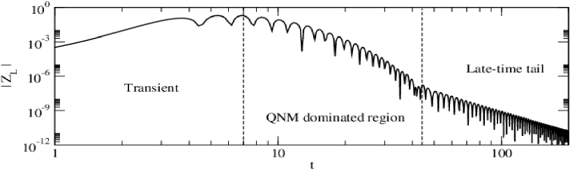
Figure 1: Log-log graph of the absolute value of $Z_{L}(t,x_{fixed})$. The quasi-normal and tail phases are indicated. The $p$-brane parameters are $p=0$, $a=2$, $b=0.5$, $L=1$ and $\beta=1$

As a conclusion, we can say that the black $p$-branes are stable against scalar and tensorial perturbations. Also, the quasi-normal spectrum in such a complex geometry is amazingly simple. Considering $\beta\neq 0$, later related to glueball mass in the AdS/CFT framework, the frequencies display an almost scaling behaviour.

4 The AdS/CFT Correspondence

The $D3$-brane metric is

$$ds^{2}=\left(1+\frac{L^{4}}{r^{4}}\right)^{-\frac{1}{2}}\left(-dt^{2}+\sum_{i=1}^{3}dx_{i}^{2}\right)+\left(1+\frac{L^{4}}{r^{4}}\right)^{\frac{1}{2}}\left(dr^{2}+r^{2}d\Omega_{5}^{2}\right)\ ,$$ (13)

where $d\Omega_{5}^{2}$ is the $5$-sphere metric and $L^{4}=4\pi g_{s}N^{2}$. In an appropriate limit, this metric can be written as

$$ds^{2}=\frac{r^{2}}{L^{2}}\left(-dt^{2}+\sum_{i=1}^{3}dx_{i}^{2}\right)+\frac{L^{2}}{r^{2}}dr^{2}+d\Omega_{5}^{2}\ .$$ (14)

With the coordinate change $r=L^{2}/u$, the metric takes the form

$$ds^{2}=\frac{L^{2}}{u^{2}}\left(-dt^{2}+\sum_{i=1}^{3}dx_{i}^{2}+du^{2}\right)+L^{2}d\Omega_{5}^{2}\ ,$$ (15)

which is the product of a $5$-dimensional AdS space with a $5$-sphere.

The conjecture stated by Maldacena says that a type IIB superstring theory on AdS${}_{5}\times$S⁵ with string coupling $g_{s}$ and a $4$-dimensional $N=4$ Super-Yang-Mills (SYM) theory with gauge group $SU(N)$ and SYM coupling $g_{YM}$ are equivalent, with $g_{s}=g_{YM}^{2}$ and $L^{4}=4\pi g_{s}N^{2}$. Consider an operator $O$ in $N=4$ SYM, as seen in [10]. A generating funcional $Z[J]$ can be obtained perturbing the lagrangian $\mathcal{L}(x)\to\mathcal{L}(x)+J(x)O(x)$ so

$$Z[J]=\left<e^{-\int d^{4}xJ(x)O(x)}\right>_{\text{CFT}}\ .$$ (16)

A deformation in the operator $O$ changes the value of $g_{YM}$. Since they are related, $g_{s}$ must also change, which is equivalent to change the boundary value of the dilaton.

Let $\psi(z,x^{\mu})$ be the dilaton, defined on the metric (4). The boundary value is written as $\psi(z=0,x^{\mu})=\psi_{0}(x^{\mu})=J(x)$. According to the AdS/CFT correspondence [19],

$$\left<e^{-\int d^{4}xJ(x)O(x)}\right>=Z_{\text{string}}\left[\psi(z,x^{\mu})=\psi_{0}(x^{\mu})\right]\ .$$ (17)

$Z_{\text{string}}$ is the partition function on the AdS space where the field $\psi$ has the value $\psi_{0}$ as boundary condition.

Returning to the free scalar fields on AdS, whose asymptotic solution if given by eq. (7), with $\Delta_{\pm}$ given by eq. (8), we choose one of the independent solution, that it, $\psi(z,x^{\mu})=\alpha(x^{\mu})z^{\Delta_{-}}$ and $\beta(x^{\mu})=0$ or $\psi(z,x^{\mu})=\beta(x^{\mu})z^{\Delta_{+}}$ and $\alpha(x^{\mu})=0$. Let $\epsilon$ be a coordinate value close to the boundary $z=0$. Then, $\psi(\epsilon,x^{\mu})=\alpha(x)\epsilon^{\Delta_{-}}$ ( or $\psi(\epsilon,x^{\mu})=\beta(x)\epsilon^{\Delta_{+}}$). $\epsilon$ has dimension $[\text{length}]^{-1}$ and $\psi$ is dimensionless. Therefore, $\alpha(x^{\mu})$ has mass dimension $\Delta_{-}$ (or $\beta(x^{\mu})$ has mass dimension $\Delta_{+}$). Since $J(x)=\alpha(x^{\mu})$ (or $J(x)=\beta(x^{\mu})$), eq. (17) implies that the operator $O$ has dimension $\Delta_{-}$ (or $\Delta_{+}$).

5 Holographic Superconductors

According to the AdS/CFT correspondence, a gravitational theory in the bulk is related to a field theory on the boundary. A space-time with a black hole is related to a thermal field theory, whose temperature is equal to the Hawking temperature of the black hole. Charged scalar fields in the bulk are related to condensates in the thermal field theory, so these scalar fields must behave like a order parameter if the thermal field theory describes a superconductivity.

Consider the lagrangian from [6]

$$\mathcal{L}=R+\frac{6}{L^{2}}-\frac{1}{4}F_{\mu\nu}^{2}-|\nabla_{\mu}\psi-iqA_{\mu}\psi|^{2}-m^{2}|\psi|^{2}\ .$$ (18)

If we rescale $\psi\to\psi/q$ and $A_{\mu}\to A_{\mu}/q$, then the matter action has a $1/q^{2}$ factor, so a large $q$ supresses the backreaction in the metric.

Considering the planar neutral black hole

$$ds^{2}=-f(r)dt^{2}+f^{-1}(r)dr^{2}+r^{2}(dx^{2}+dy^{2})\ ,$$ (19)

where

$$f(r)=\frac{r^{2}}{L^{2}}-\frac{M}{r}\qquad\text{and}\qquad T=\frac{3r_{h}}{4\pi L^{2}}=\frac{3}{4\pi}\frac{M^{\frac{1}{3}}}{L^{\frac{4}{3}}}\ ,$$ (20)

we assume that the fields depend only on the radial coordinate $A_{\mu}dx^{\mu}=\Phi(r)dt$, $\psi=\psi(r)$. Then the field equations for $m^{2}L^{2}=-2$ become

$$\psi^{\prime\prime}+\left(\frac{f^{\prime}}{f}+\frac{2}{r}\right)\psi^{\prime}+\frac{\Phi^{2}}{f^{2}}\psi+\frac{2}{L^{2}f}\psi=0\ ,$$ (21)

$$\Phi^{\prime\prime}+\frac{2}{r}\Phi^{\prime}-\frac{2\psi^{2}}{f}\Phi=0\ .$$ (22)

At the event horizon $r=r_{h}$, the equations of motion are regular if $\phi(r_{h})=0$ and $f^{\prime}(r_{h})\psi^{\prime}(r_{h})+\frac{2}{L^{2}}\psi(r_{h})=0$. So, there is a two parameter family of solutions with regular horizons. Asymptotically,

$$\psi = \frac{\psi^{(1)}}{r}+\frac{\psi^{(2)}}{r^{2}}+\cdots\ ,$$ (23)

$$\Phi = -\mu-\frac{\rho}{r}+\cdots\ .$$ (24)

To understand the asymptotic behaviour of $\Phi(r)$, consider a charged black hole perturbation. The time component of the electromagnetic potential behaves as a power law decay next to the AdS boundary and does not correspond to a field in the dual theory, but fixes the charge density $\rho$ of a state. This component must be zero at the event horizon, so a constant must be added, which can be understood in the dual field theory as a sum of a chemical potential $\mu$.

For $\psi$, either falloff if normalizable. We need to impose the condition that either $\psi^{(1)}$ or $\psi^{(2)}$ vanishes. To do so, for each pair of boundary conditions $(\psi(r_{h}),\Phi(r_{h}))$ we numerically solve eqs. (21) and (22) using fourth order Runge-Kutta method and for large $r$, fit the behaviour os $\psi(r)$ and $\Phi(r)$ as eqs. (23) and (24), which are linear on the parameters. This procedure gives us a map $(\psi(r_{h}),\Phi(r_{h}))\to(\psi^{(1)},\psi^{(2)},\mu,\rho)$. Using the shooting method, we find the pair of boundary conditions for which $\psi^{(1)}$ or $\psi^{(2)}$ vanishes. When $\psi^{(2)}=0$, we plot $<O_{1}>=\sqrt{2}\psi^{(1)}$ against $T$ and when $\psi^{(1)}=0$, $<O_{2}>=\sqrt{2}\psi^{(2)}$ against $T$.

At this point, is important to mention that equations of motion for the charged scalar field $\psi$ and electric potential $\Phi$ are invariant under two groups of scaling symmetries. The first one ($r\rightarrow\lambda r$, $t\rightarrow\lambda t$, $L\rightarrow\lambda L$, $q\rightarrow\lambda^{-1}q$, $m\rightarrow\lambda^{-1}m$), allow us to set the value of AdS radius $L=1$. The second one ($r\rightarrow\lambda r$, $t\rightarrow\lambda^{-1}t$, $\Phi\rightarrow\lambda^{-1}\Phi$), we can take $r_{h}=1$, which implies that the Hawking temperature is $T=3/4\pi$. Furthermore, the two groups of symmetry imply $T\rightarrow\lambda^{2}T$, and $\rho\rightarrow\lambda^{2}\rho$. From this, we see that $T\propto\rho^{1/2}$. Therefore, we can do calculations with $r_{h}=1$ and evaluate $T/\rho^{1/2}$ to eliminate the scaling symmetries that we used to set $r_{h}=1$.

Several curves appear, and they can be labelled by the number of times that $\psi(r)$ changes signal. Taking only cases in which $\psi(r)$ does not change signal, the figures in [6] are obtained.

$\psi(r)$ behaves like a order parameter, but this behaviour alone is not enough to see if the phase transition is that of a superconductor or a superfluid. We need then to obtain the conductivity $\sigma(\omega)$, where $\omega$ is the frequency. Perturbing the spatial component of the electromagnetic potential $A_{x}$ and assuming $A_{x}(r,t)=e^{-i\omega t}A_{x}(r)$, we get

$$A_{x}^{\prime\prime}+\frac{f^{\prime}}{f}A_{x}^{\prime}+\left(\frac{\omega^{2}}{f^{2}}-\frac{2\psi^{2}}{f}\right)A_{x}=0\ .$$ (25)

As $r\to r_{h}$, $A_{x}\to f^{-\frac{i\omega}{3r_{h}}}$. As $r\to\infty$,

$$A_{x}\simeq A_{x}^{(0)}+\frac{A_{x}^{(1)}}{r}+\cdots\ .$$ (26)

According to [3], the AdS/CFT dictionary says that the electric field in the CFT is equal to the electric field in the bulk as $r$ tends to infinity ($E_{x}=-\dot{A}_{x}^{(0)}$), and the first subleading term is dual to the induced current ($<J_{x}>=A_{x}^{(1)}$). Applying Ohm’s law,

$$\sigma(\omega)=\frac{<J_{x}>}{E_{x}}=-\frac{i}{\omega}\frac{A_{x}^{(1)}}{A_{x}^{(0)}}\ ,$$ (27)

whose behaviour is presented in [6]. For temperatures higher than the critical temperature, the real part of the conductivity is constant. For lower temperatures, there is a energy gap, as expected by BCS theory.

6 Phase transitions in Reissner-Nordström holographic superconductors

We consider the bulk action of a massive charged scalar field $\psi$ interacting with an abelian field $A_{\mu}$ generated by a charged AdS black hole, as in [4]. We keep the lagrangian (18) and now the background space-time is a spherically symmetric Reissner-Nordström AdS black hole

$$ds^{2}=-f(r)dt^{2}+\frac{1}{f(r)}dr^{2}+r^{2}d\Omega^{2}$$ (28)

with

$$f(r)=1-\frac{2M}{r}+\frac{Q^{2}}{4r^{2}}+\frac{r^{2}}{L^{2}}\ .$$ (29)

The abelian field is now fixed, $A_{\mu}dx^{\mu}=\Phi(r)dt$ with

$$\Phi(r)=\frac{Q}{r}-\frac{Q}{r_{+}}\ .$$ (30)

Assuming that $\psi$ depends only on $r$, the equation of motion is

$$\frac{1}{\sqrt{-g}}\partial_{r}\left(\sqrt{-g}g^{rr}\partial_{r}\psi\right)-\left(m^{2}-\frac{q^{2}\Phi^{2}(r)}{f(r)}\right)\psi=0\ .$$ (31)

Choosing coordinates in which $r_{+}=Q=1$, the Hawking temperature is given by

$$T=\frac{3}{4\pi}\left(\frac{1}{4}+\frac{1}{L^{2}}\right)$$ (32)

and eq. (31) depends only on the parameters $m$, $q$ and $L$.

We can set the boundary condition $\psi(r=1)=1$, since the equation of motion is linear. Developing a series solution around the horizon, we find $\psi^{\prime}(r=1)=\frac{4m^{2}L^{2}}{3L^{2}+12}$. With these conditions, we can numerically solve eq. (31) using fourth order Runge-Kutta method and search parameters for which $\psi\to 0$ as $r\to\infty$. Fixing $m^{2}L^{2}=4$ and $qL=10$, we need to vary only the parameter $L$, making the search straightforward. There are only three values of $L$ for which $\psi$ tends to zero, shown in figure 2. These modes can be labelled by the number of times $\psi$ changes signal and are called marginally stable modes.

Keeping the same fixed abelian field, but letting now $\psi$ depend on time as well as the radial coordinate, we have the following equation of motion,

$$\square\psi-2iqA_{\mu}g^{\mu\nu}\partial_{\nu}\psi-q^{2}A_{\mu}A^{\mu}\psi-m^{2}\psi\ .$$ (33)

With the Ansatz $A_{\mu}dx^{\mu}=\Phi(r)dt$ and the tortoise coordinate $r_{\star}(r)=\int\frac{dr}{f(r)}$, we write the equation por $\psi(r,t)$ as

$$-\frac{\partial^{2}\psi}{\partial t^{2}}+\frac{\partial^{2}\psi}{\partial r_{\star}^{2}}+2iq\Phi(r)\frac{\partial\psi}{\partial t}-V_{\text{eff}}(r)\psi=0$$ (34)

with

$$V_{\text{eff}}(r)=f(r)\left(\frac{f^{\prime}(r)}{r}+m^{2}\right)-q^{2}\Phi^{2}(r)\ ,$$ (35)

which is the equation for a charged scalar perturbation of the Reissner-Nordström-AdS black hole with an aditional imaginary term.

According to the AdS/CFT correspondence, a black hole is related to a thermal field theory, perturbations of the black hole are perturbations of the thermal theory and the imaginary part of the quasi-normal frequencies is related to the timescale of the return to thermal equilibrium [14]. For a condensate not to decay in the dual field theory, there must be an unstable quasi-normal mode in the bulk and the phase transition must happen at the same temperature that the quasi-normal modes change stability.

Fitting the behaviour of the quasi-normal modes as $\psi(r,t)=e^{-i\omega t}\psi(r)$ and, if the frequency is zero, as the imaginary part must be when the mode changes stability, it is easy to see that the transition must happen at a marginally stable mode. At this point the meaning of more than one marginally stable mode is not clear.

We must now solve eq. (34) numerically. With a gaussian distribution as initial condition and Dirichlet condition at $r_{\star}=0$, we derive the evolution of $\psi(r,t)$ using the finite difference method. As in the case of marginally stable modes, we choose coordinates in which $r_{+}=Q=1$ and fix $m^{2}L^{2}=4$ and $qL=10$ so the system depends only on one parameter $L$, which has a biunivocal relation with the Hawking temperature given by eq. (32).

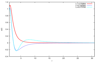
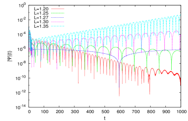
Figure 2: Marginally stable modes (left) and quasi-normal modes near the transition (right)

As can be seen in figure 2, there is indeed a stability change, and the transition occurs at $L\sim 1.28$, which is the first marginally stable mode. In figure 4, we show the real and imaginary parts of the quasi-normal frequency. Both parts change signal at the same value of $L$.

For values of $L$ close to the second marginally stable mode, $\psi(r,t)$ behaves as a superposition of two oscilations with distinct frequencies. Figure 3 shows $\psi(r,t)$ and the extracted second mode. The second mode exhibits a transition at $L\sim 2.15$, which is the second marginally stable mode. The frequencies are shown in figure 4. Since there is a third marginally stable mode, we assume that there is a third quasi-normal mode, but our analysis could not see it, as it is small compared to the other quasi-normal modes.

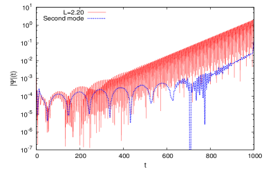
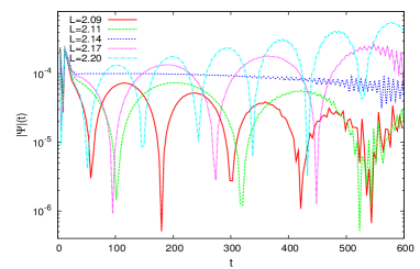
Figure 3: Extracted secondary quasi-normal mode (left) and secondary quasi-normal modes for values of $L$ near the second marginally stable mode (right).

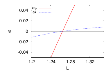
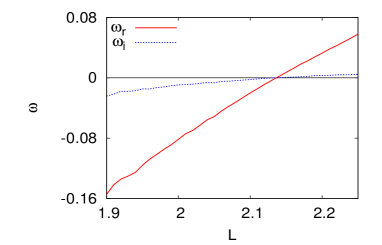
Figure 4: Quasi-normal frequencies of fundamental mode (left) and of the extracted secondary mode (right).

We can conclude now that the existence of more than one marginally stable mode means that there are more than one quasi-normal mode that changes stability at a particular marginally stable mode. For the system to be stable, all quasi-normal modes must be stable, and when one single quasi-normal mode changes stability, the whole system is unstable. So there is only one phase transition, which happens at the marginally stable mode labelled as fundamental. This work has been published in [5].

- [1] J. Maldacena, The Large N Limit of Superconformal Field Theories and Supergravity, Adv. Theor. Math. Phys. 2 (1998) 231 [hep-th/9711200].
- [2] E. Witten, Anti De Sitter Space And Holography, Adv. Theor. Math. Phys. 2 (1998) 253 [hep-th/9802150].
- [3] G. T. Horowitz, Introduction to Holographic Superconductors [hep-th/1002.1722].
- [4] S. S. Gubser, Breaking an Abelian gauge symmetry near a black hole horizon Phys. Rev. D 78 (2008) 065034 [hep-th/0801.2977].
- [5] E. Abdalla, C. E. Pellicer, J. Oliveira and A. B. Pavan, Phase transitions and regions of stability in Reissner-Nordström holographic superconductors, Phys. Rev. D 82 (2010) 124033 [hep-th/1010.2806].
- [6] S. A. Hartnoll, C. P. Herzog, and G. T. Horowitz, Building an AdS/CFT superconductor, Phys. Rev. Lett. 101 (2008) 031601 [hep-th/0803.3295].
- [7] G. ’t Hooft, Dimensional Reduction in Quantum Gravity, [gr-qc/9310026].
- [8] L. Susskind, The World as a Hologram, J. Math. Phys. 36 (1995) 6377 [hep-th/9409089].
- [9] H. Nastase, Introduction to AdS-CFT, [hep-th/0712.0689].
- [10] J. McGreevy, Holographic duality with a view toward many-body physics, [hep-th/0909.0518].
- [11] K. D. Kokkotas and B. Schmidt, Quasi-Normal Modes of Stars and Black Holes, Living Rev. Relativity 2 (1999).
- [12] H.-P. Nollert, Quasinormal modes: the characteristic ‘sound’ of black holes and neutron stars, Class. Quantum Grav. 16 (1999) R159.
- [13] R. M. Wald, Note on the stability of the Schwarzschild metric, J. Math. Phys. 20 (1979) 1056.
- [14] G. T. Horowitz and V. E. Hubeny, Quasinormal modes of AdS black holes and the approach to thermal equilibrium, Phys. Rev. D 62 (2000) 024027. [hep-th/9909056].
- [15] A. Bachelot e A. Motet-Bachelot, Les résonances d’un trou noir de Schwarzschild., Ann. Inst. Henri Poincaré 59 (1993) 3-68.
- [16] G. W. Gibbons and P. K. Townsend, Vacuum interpolation in supergravity via super p-branes, Phys. Rev. Lett. 71 (1993) 3754 [hep-th/9307049].
- [17] E. Abdalla, O. P. F. Piedra and J. de Oliveira, C. Molina Perturbations of black p-branes, Phys. Rev. D 81 (2010) 064001 [hep-th/0810.5489].
- [18] H. Kodama, A. Ishibashi, A master equation for gravitational perturbations of maximally symmetric black holes in higher dimensions, Prog. Theor. Phys. 110 (2003) 701 [hep-th/0305147].
- [19] O. Aharony, S. S. Gubser, J. Maldacena, H. Ooguri and Y. Oz, Large N Field Theories, String Theory and Gravity, Phys.Rept. 323 (2000) 183-386 [hep-th/9905111].