Lorentzian area measures and the Christoffel problem

Abstract

We introduce a particular class of unbounded closed convex sets of ${\mathbb{R}}^{d+1}$, called F-convex sets (F stands for future). To define them, we use the Minkowski bilinear form of signature $(+,\ldots,+,-)$ instead of the usual scalar product, and we ask the Gauss map to be a surjection onto the hyperbolic space ${\mathbb{H}}^{d}$. Important examples are embeddings of the universal cover of some globally hyperbolic maximal flat Lorentzian manifolds.

Basic tools are first derived, similarly to the classical study of convex bodies. For example, F-convex sets are determined by their support function, which is defined on ${\mathbb{H}}^{d}$. Then the area measures of order $i$, $0\leq i\leq d$ are defined. As in the convex bodies case, they are the coefficients of the polynomial in $\varepsilon$ which is the volume of an $\varepsilon$ approximation of the convex set. Here the area measures are defined with respect to the Lorentzian structure.

Then we focus on the area measure of order one. Finding necessary and sufficient conditions for a measure (here on ${\mathbb{H}}^{d}$) to be the first area measure of an F-convex set is the Christoffel Problem. We derive many results about this problem. If we restrict to F-convex set setwise invariant under linear isometries acting cocompactly on ${\mathbb{H}}^{d}$, then the problem is totally solved, analogously to the case of convex bodies. In this case the measure can be given on a compact hyperbolic manifold.

Particular attention is given on the smooth and polyhedral cases. In those cases, the Christoffel problem is equivalent to prescribing the mean radius of curvature and the edge lengths respectively.

Université de Cergy-Pontoise, UMR CNRS 8088, F-95000 Cergy-Pontoise, France.

Universite Paris 13, Sorbonne Paris Cité, LAGA, CNRS (UMR 7539), F-93430 Villetaneuse, France.

francois.fillastre@u-cergy.fr, veronelli@math.univ-paris13.fr

MSC: 52A38, 52A38, 58J05

1 Introduction

1.1 Area measures and the Christoffel problem for convex bodies

Let $K$ be a convex body in $\mathbb{R}^{d+1}$ and $\omega$ be a Borel set of the sphere $\mathbb{S}^{d}$, seen as the set of unit vectors of $\mathbb{R}^{d+1}$. Let $B_{\varepsilon}(K,\omega)$ be the set of points $p$ which are at distance as most $\varepsilon$ from their metric projection $\overline{p}$ onto $K$ and such that $p-\overline{p}$ is collinear to a vector belonging to $\omega$. It was proved in [FJ38] that the volume of $B_{\varepsilon}(K,\omega)$ is a polynomial with respect to $\varepsilon$:

$$V(B_{\varepsilon}(K,\omega))=\frac{1}{d+1}\sum_{i=0}^{d}\varepsilon^{d+1-i}\binom{d+1}{i}S_{i}(K,\omega).$$ (I)

Each $S_{i}(K,\cdot)$ is a finite positive measure on the Borel sets of the sphere, called the area measure of order $i$. $S_{0}(K,\cdot)$ is only the Lebesgue measure of the sphere $\mathbb{S}^{d}$, and $S_{d}(K,\omega)$ is the $d$-dimensional Hausdorff measure of the pre-image of $\omega$ for the Gauss map. The problem of prescribing the $d$th area measure is the (generalized) Minkowski problem, and the one of prescribing the first area measure is the (generalized) Christoffel problem (each problem having a smooth and polyhedral specialized version).

There are other ways of introducing the area measures [Sch93a]. If $K_{\varepsilon}:=K+\varepsilon B$, with $B$ the unit closed ball, we have

$$S_{d}(K_{\varepsilon},\omega)=\sum_{i=0}^{d}\varepsilon^{d-i}\binom{d}{i}S_{i}(K,\omega).$$ (II)

We can also use the mixed-volume $V(\cdot,\ldots,\cdot)$. Let $h_{K}$ be the support function of $K$:

$$h_{K}(x)=\sup_{k\in K}\langle x,k\rangle$$

where $\langle\cdot,\cdot\rangle$ is the usual scalar product and $x\in\mathbb{S}^{d}$. The set of support functions of convex bodies in $\mathbb{R}^{d}$ is a convex cone, that spans a linear subspace of the space of continuous functions on $\mathbb{S}^{d}$. Identifying a convex body with its support function, the mixed-volume is the unique symmetric $(d+1)$-linear form on the space of convex bodies of $\mathbb{R}^{d+1}$ with $V(K,\ldots,K)=V(K)$, if $V$ is the volume. It is continuous and hence, fixing convex bodies $K_{1},\ldots,K_{d}$, $V(K,K_{1},\ldots,K_{d})$, seen as a function of $h_{K}$, is an additive functional on a subset of the space of continuous functions on the sphere $\mathbb{S}^{d}$. It can be extended to the whole space, and by the Riesz representation theorem, there exists a unique measure $S(K_{1},\ldots,K_{d};\cdot)$ on the Borel sets of the sphere with

$$V(K,K_{1},\ldots,K_{d})=\frac{1}{d+1}\int_{\mathbb{S}^{d}}h_{K}(x)\mathrm{d}S(K_{1},\ldots,K_{d},x).$$

The area measure of order $i$ can then be defined as

$$S_{i}(K,\cdot)=S(\underbrace{K,\ldots,K}_{i},B,\ldots,B,\cdot),$$

so the first area measure of $K$ is the unique positive measure on the sphere such that for any convex body $K^{\prime}$,

$$V(K^{\prime},K,B,\ldots,B)=\frac{1}{d+1}\int_{\mathbb{S}^{d}}h_{K^{\prime}}(x)\mathrm{d}S_{1}(K,x).$$ (III)

A last way of defining the first area measure is due to C. Berg [Ber69]. In the case of a strictly convex body with $C^{2}$ boundary $K$, the first area measure is $\varphi_{K}\mbox{d}\mathbb{S}^{d}$, with $\mbox{d}\mathbb{S}^{d}$ the usual volume form on the sphere and $\varphi_{K}$ the mean radius of curvature of $K$ (the sum of the principal radii of curvature of $\partial K$ divided by $d$). One can compute $\varphi_{K}$ as

$$\frac{1}{d}{}^{\mathbb{S}^{d}}\!\!\!\Delta h_{K}+h_{K}$$ (IV)

where ${}^{\mathbb{S}^{d}}\!\!\!\Delta$ is the Laplacian on $\mathbb{S}^{d}$. The fact is that, for any convex body $K$, $S_{1}(K,\cdot)$ is equal in the sense of distributions to the formula above, defined in the sense of distributions. All those definitions of area measures use approximation results of a convex body by a sequence of polyhedral or smooth convex bodies.

The Christoffel problem was completely solved independently by W. Firey (for sufficiently smooth case in [Fir67], then generally by approximation in [Fir68]) and C. Berg [Ber69]. See [Fir81] for an history of the problem to the date, and Section 4.3 in [Sch93a]. See [GZ99], [GYY11] for developments around [Ber69].

1.2 Content of the paper

There is an active research about problems à la Minkowski and Christoffel for space-like hypersurfaces of the Minkowski space (at least too many to be cited exhaustively; some references will be given further). However they mainly concern smooth hypersurfaces, and often in the $d=2$ case. One of the aim of the present paper is to introduce a class of convex set which are intended to be the analog of convex bodies when the Euclidean structure is considered. In particular, they are the objects arising naturally for this kind of problems.

In the first section of the paper we define F-convex sets. They are intersection of the future sides of space-like hyperplanes, such that any future time-like vector is a support vector of the convex set. This section is almost self-contained, as we have to prove all the basics results similar to the convex bodies theory, for which the main source was [Sch93a]. Actually we will use some results contained in [Bon05]. For example, the support functions of F-convex sets are defined on ${\mathbb{H}}^{d}$. Also, single points, which are convex bodies, are not F-convex bodies. Their analogues are future cones of single points. However the matter is complicated because conditions on the boundary enter the picture (F-convex sets may have light-like support planes).

The motivation behind the definition of F-convex set is to be able to get the analog of (I) for the Lorentzian structure. The volume is independent of the signature of the metric, but not the orthogonal projection. The idea is to first prove it for particular F-convex sets, called Fuchsian convex sets which are F-convex sets invariant under a group of linear isometries $\Gamma$ of the Minkowski space acting cocompactly on ${\mathbb{H}}^{d}\subset{\mathbb{R}}^{d+1}$. In many aspects they behave very analogously to convex bodies, roughly speaking compactness is replaced by “cocompactness” (this was noted in [Fil13]). For them, we find formulas analogous to (I) and (III). As the definition of area measure is local, we use a result of “Fuchsian extension” (Subsection 3.3) of any part of an F-convex set to treat the general case.

We then focus on the first area measure. In the regular case, it is absolutely continuous with respect to the volume form of ${\mathbb{H}}^{d}$ with density the mean radius of curvature $\varphi$, obtained as

$$\frac{1}{d}\Delta h-h=\varphi$$ (1)

where $\Delta$ is the Beltrami–Laplace operator on $\mathbb{H}^{d}$. In the general case, the area measure of order one is given by the formula above in the sense of distribution.

To find conditions on a given measure $\mu$ on ${\mathbb{H}}^{d}$ such that there exists an F-convex set with $\mu$ as first area measure is the Christoffel problem. Section 4 contains computations related to the Christoffel problem. In the smooth case, related results were proved in [Sov81, Sov83, OS83, LdLSdL06]. Our computations go back to [Hel59, Hel62], and generalizes the preceding ones. See Remark 4.2 for more details. In the polyhedral case, we adapt a classical construction, which appears to be related to more recent works on Lorentzian geometry [Mes07, Bon05, BB09], see Remark 4.14.

The content of Section 5 will be described later.

1.3 The Fuchsian case

Fuchsian convex sets are very special F-convex sets, because they are at the same time invariant under the action of a (cocompact) group and contained in the future cone of a point, which is a relevant property as it will appear. Seemly, they are the only F-convex sets for which a definitive result can be given, very analogous to the one of convex bodies. By invariance, the support function of Fuchsian convex bodies can be defined on the compact hyperbolic manifold ${\mathbb{H}}^{d}/\Gamma$ instead of ${\mathbb{H}}^{d}$. The following statement stands to give an idea about the kind of results we obtained, we cannot define precisely all the terms in the introduction.

Theorem 1.1.

Let $\Gamma$ be so that $\mathbb{H}^{d}/\Gamma$ is a compact hyperbolic manifold with universal covering map $P_{\Gamma}:\mathbb{H}^{d}\to\mathbb{H}^{d}/\Gamma$. Let $\bar{\mu}$ be a positive Radon measure on $\mathbb{H}^{d}/\Gamma$. Define a positive Radon measure $\mu:=P_{\Gamma}^{\ast}\bar{\mu}$ on $\mathbb{H}^{d}$ as the pull-back distribution of $\bar{\mu}$ (see Subsection 4.3) and define the distribution

$$h_{\mu}:=\int_{\mathbb{H}^{d}}G(x,y)\mathrm{d}\mu(y)$$

where $G(x,y)$ is the kernel function defined by

$$G(x,y)=\frac{\cosh d_{\mathbb{H}^{d}}(x,y)}{v_{d-1}}\int_{+\infty}^{d_{\mathbb{H}^{d}}(x,y)}\frac{\mathrm{d}t}{\sinh^{d-1}(t)\cosh^{2}(t)}$$

($v_{d-1}$ is the area of $\mathbb{S}^{d-1}\subset{\mathbb{R}}^{d}$) and the precise action of $h_{\mu}$ is explained in (58). Then

1. $h_{\mu}$ is a solution to equation

   $$\frac{1}{d}\Delta h-h=\mu$$

   in the sense of distributions on $\mathbb{H}^{d}$.

2. There exists a unique $\Gamma$-invariant F-convex set $K$ with first area measure $\bar{\mu}$ if and only if

   1. $$\left|\int_{\mathbb{H}^{d}}G(x,y)\mathrm{d}\mu(y)\right|<+\infty,\quad\forall x\in{\mathbb{H}}^{d},$$

   2. the convexity condition

      $$\int_{\mathbb{H}^{d}}\Lambda(\eta,\nu,y)\mathrm{d}\mu(y)\geq 0,$$

      is satisfied for all future time-like vectors $\eta,\nu$, where $\Lambda(\eta,\nu,y)$ is

      $$\Lambda(\eta,\nu,y)=\Gamma(\eta,y)+\Gamma(\nu,y)-\Gamma(\eta+\nu,y)$$

      and $\Gamma(\eta,y)=\|\eta\|_{-}G\left(\frac{\eta}{\|\eta\|_{-}},y\right)$.

3. If $\mu=\bar{\varphi}\mathrm{d}{\mathbb{H}}^{d}$ for some $0<\bar{\varphi}\in C^{k,\alpha}({\mathbb{H}^{d}/\Gamma})$, $k\geq 0$ and $0\leq\alpha<1$, then $h_{\mu}\in C^{k+2,\alpha}(\mathbb{H}^{d})$ if $\alpha>0$ and $h_{\mu}\in C^{1,\beta}(\mathbb{H}^{d})$ for all $\beta<1$ if $\alpha=k=0$.

If the $\bar{\varphi}$ above is $C^{2}$ another characterization of convexity is given in Proposition 4.18. In this case $\bar{\varphi}$ is the mean radius of curvature of the Fuchsian convex set with support function $h_{\mu}$.

Those conditions are very cumbersome, so necessary conditions could be wished. In the compact Euclidean case, necessary conditions were first given in [Pog53, Pog73] (a proof is in [GM03]), but it does not seem to have an analogue in our case, see Remark 4.20, and the next subsection.

1.4 Quasi-Fuchsian convex sets and flat spacetimes

A quasi-Fuchsian convex set is the data of an F-convex set $K$ and a group of isometries $\Gamma$ of the Minkowski space such that

• $K$ is setwise invariant under the action of $\Gamma$,

• $\Gamma$ is isomorphic to its linear part $\Gamma_{0}$, which is such that ${\mathbb{H}}^{d}/\Gamma_{0}$ is a compact hyperbolic manifold.

Their interest comes in part from general relativity. Actually for any group $\Gamma$ as above, there is a unique convex open set $\Omega$, maximal for the inclusion, such that $\Gamma$ acts freely properly discontinuously on it. The closure of $\Omega$ is an F-convex set. The quotient $\Omega/\Gamma$ is a future complete flat Lorentzian spacetime, globally hyperbolic, maximal, spatially compact and homeomorphic to ${\mathbb{H}}^{d}/\Gamma_{0}\times{\mathbb{R}}$. We refer to [Bar05] for a classification of such manifolds. For more details on $\Omega$, see [Mes07, ABB⁺07, Bon05, BB09].

Section 5 contains in particular a kind of slicing of those spacetimes by constant mean radius of curvature hypersurface (the “dual” problem of slicing by constant mean curvature hypersurfaces is classical, see [ABBZ12]), with the particularity that the slicing goes “outside” of the future complete space-time and then slices a past complete spacetime.

1.5 The Christoffel–Minkowski problem

From now on let us consider only smooth objects. The classical Christoffel–Minkowski problem consists of characterizing functions on the sphere which are elementary symmetric functions of the radii of curvature of convex bodies. Aside from the cases corresponding to the Minkowski and Christoffel problems, the Christoffel–Minkowski problem is not yet solved. Active research is still going on, see [STW04, GM03, GLM06, GMZ06] and the references inside (see [GLL12] for the “dual” problem of prescribing curvature measures). Another aim of the present paper is to bring attention to the fact that similar analysis can be done on the hyperbolic space or on compact hyperbolic manifolds, that still have a geometric interpretation. Convex bodies are then replaced by F-convex sets.

For example, a Minkowski theorem (smooth version) was proved for quasi-Fuchsian convex sets in [BBZ11], in the case $d=2$. In the Fuchsian case, it is proved in any dimension [OS83]. The Minkowski problem for quasi-Fuchsian convex sets is the subject of [BF14].

1.6 Acknowledgement

The authors want to thank Francesco Bonsante, Thierry Daudé, Gerasim Kokarev, Yves Martinez-Maure and Jean-Marc Schlenker. The first author enjoyed useful conversations with Yves Martinez-Maure about hedgehogs. Francesco Bonsante pointed out to the first author the relation between the first area measure and measured geodesic laminations.

Several remarks and suggestions from the anonymous referee contributed to improve both the content and the presentation of this paper. The authors are grateful to him for such a careful reading.

The first author was partially supported by the ANR GR-Analysis-Geometry. The second author was partially supported by INdAM COFUND-2012 Outgoing Fellowships in Mathematics and/or Applications Cofunded by Marie Curie Actions.

2 Background on convex sets

2.1 Notations

Subsets of ${\mathbb{R}}^{d+1}$.

For a set $A\subset{\mathbb{R}}^{d+1}$ we will denote by $\overline{A},\stackrel{{\scriptstyle\circ}}{{A}},\partial A$ respectively the closure, the interior and the boundary of $A$. A hyperplane $\mathcal{H}$ of ${\mathbb{R}}^{d+1}$ is a support plane of a closed convex set $K$ if it has a non empty intersection with $K$ and $K$ is totally contained in one side of $\mathcal{H}$. In this paper, a vector orthogonal to a support plane and inward pointing is a support vector of $K$. A support plane at infinity of $K$ is a hyperplane $\mathcal{H}$ such that $K$ is contained in one side of $\mathcal{H}$, and any parallel displacement of $\mathcal{H}$ in the direction of $K$ meets the interior of $K$ ($\mathcal{H}$ and $K$ may have empty intersection). A support plane is a support plane at infinity.

We denote by $V$ the volume form of ${\mathbb{R}}^{d+1}$ (the Lebesgue measure).

Minkowski space.

The Minkowski space-time of dimension $(d+1)$, $d\geq 1$, is $\mathbb{R}^{d+1}$ endowed with the symmetric bilinear form

$$\langle x,y\rangle_{-}=x_{1}y_{1}+\cdots+x_{n}y_{n}-x_{d+1}y_{d+1}.$$

The interior of the future cone of a point $p$ is denoted by $I^{+}(p)$. We will denote $I^{+}(0)$ by $\mathcal{F}$, it is the set of future time-like vectors:

$${\mathcal{F}}=\{x\in{\mathbb{R}}^{d+1}|\langle x,x\rangle_{-}<0,x_{d+1}>0\}.$$

$\partial{\mathcal{F}}^{\star}$ and $\overline{{\mathcal{F}}}^{\star}$ are respectively $\partial{\mathcal{F}}$ and $\overline{{\mathcal{F}}}$ without the origin (respectively the set of future light-like vectors and the set of future vectors). Let us also denote

$${\mathcal{C}}(p):=\overline{I^{+}(p)}$$

and for $t>0$,

$$K({\mathbb{H}}_{t}):=\{x\in{\mathbb{R}}^{d+1}|\langle x,x\rangle_{-}\leq-t^{2},x_{d+1}>0\}$$

with $K({\mathbb{H}}):=K({\mathbb{H}}_{1})$.

For a differentiable real function $f$ on an open set of $\mathbb{R}^{d+1}$, $\operatorname{grad}_{x}f$ will be the Lorentzian gradient of $f$ at $x$:

$$D_{x}f(X)=\langle X,\operatorname{grad}_{x}f\rangle_{-},$$

namely the Lorentzian gradient is the vector with entries $(\frac{\partial f}{\partial x_{1}},\ldots,\frac{\partial f}{\partial x_{d}},-\frac{\partial f}{\partial x_{d+1}})$.

For two points $x,y$ on a causal (i.e. no-where space-like) line, the Lorentzian distance is

$$d_{L}(x,y)=\sqrt{-\langle x-y,x-y\rangle_{-}},$$

and $\|x\|_{-}:=d_{L}(x,0).$ We have the reversed triangle inequality:

$$\|x\|_{-}+\|y\|_{-}\leq\|x+y\|_{-},\qquad\forall x,y\in{\mathcal{F}}.$$ (2)

An isometry $f$ of the Minkowski space has the form $f(x)=l(x)+v$, with $v\in{\mathbb{R}}^{d+1}$ and $l\in O(d,1)$, the group of linear maps such that $lJl=J$, with

$$J=\mathrm{diag}(1,\ldots,1,-1).$$

We refer to [O’N83] for more details. For a $C^{2}$ function $f:{\mathbb{R}}^{d+1}\rightarrow{\mathbb{R}}$, the wave operator is

$$\square f=\frac{\partial^{2}f}{\partial x_{1}^{2}}+\ldots+\frac{\partial^{2}f}{\partial x_{d}^{2}}-\frac{\partial^{2}f}{\partial x_{d+1}^{2}}.$$

Hyperbolic Geometry.

In all the paper, the hyperbolic space is identified with the pseudo-sphere

$${\mathbb{H}}^{d}=\{x\in{\mathbb{R}}^{d+1}|\langle x,x\rangle_{-}=-1,x_{d+1}>0\},$$

i.e. ${\mathbb{H}}^{d}=\partial K({\mathbb{H}})$. We denote by $g,\nabla,\nabla^{2},\Delta=\operatorname{div}\nabla$ respectively the Riemannian metric, the gradient, the Hessian and the Laplacian of ${\mathbb{H}}^{d}$. Using hyperbolic coordinates on ${\mathcal{F}}$ (any orthonormal frame $X_{1},\ldots,X_{d}$ on ${\mathbb{H}}^{d}$ extended to an orthonormal frame of ${\mathcal{F}}$ with the decomposition $r^{2}g_{{\mathbb{H}}^{d}}-\mathrm{d}r\otimes\mathrm{d}r$ of the metric on ${\mathcal{F}}$), the Hessian of a function $f$ on ${\mathcal{F}}$ and the hyperbolic Hessian of its restriction to ${\mathbb{H}}^{d}$ are related by

$$\operatorname{Hess}f=\nabla^{2}f-\frac{\partial f}{\partial r}g.$$ (3)

A function $H$ on ${\mathcal{F}}$ is positively homogeneous of degree one, or in short $1$-homogeneous, if

$$H(\lambda\eta)=\lambda H(\eta)\,\forall\lambda>0.$$

It is determined by its restriction $h$ to ${\mathbb{H}}^{d}$ via $H(\eta)=h(\eta/\|\eta\|_{-})/\|\eta\|_{-}$. A function $H$ obtained in this way will be called the $1$-extension of $h$.

Lemma 2.1.

Let $h$ be a $C^{1}$ function on ${\mathbb{H}}^{d}$ and $H$ be its $1$-extension to ${\mathcal{F}}$. Then

$$\mathrm{grad}_{\eta}H=\nabla_{\eta}h-h(\eta)\eta.$$ (4)

Moreover, if $h$ is $C^{2}$, then $\forall X,Y\in T_{\eta}{\mathbb{H}}^{d}$,

$$\operatorname{Hess}_{\eta}H(X,Y)=\nabla^{2}h(X,Y)-hg(X,Y),$$ (5)

and, for $\eta\in{\mathbb{H}}^{d}$,

$$\square_{\eta}H=\Delta h-dh.$$

See Figure 7 for a geometric interpretation of (4).

Proof.

Using hyperbolic coordinates on ${\mathcal{F}}$, $\mathrm{grad}_{\eta}H$ has $d+1$ entries, and, at $\eta\in{\mathbb{H}}^{d}$, the $d$ first ones are the coordinates of $\nabla_{\eta}h$. We identify $\nabla_{\eta}h\in T_{\eta}{\mathbb{H}}^{d}\subset\mathbb{R}^{d+1}$ with a vector of $\mathbb{R}^{d+1}$. The last component of $\mathrm{grad}_{\eta}H$ is $-\partial H/\partial r(\eta)$, and, using the homogeneity of $H$, it is equal to $-h(\eta)$ when $\eta\in\mathbb{H}^{d}$. Note that at such a point, $T_{\eta}{\mathcal{F}}$ is the orthogonal sum of $T_{\eta}\mathbb{H}^{d}$ and $\eta$, and (4) follows.

On the other hand, $\nabla^{2}h(X,Y)=g(D_{X}\nabla h,Y)$, with $X,Y\in T_{\eta}{\mathbb{H}}^{d}$, where $D$ is the Levi-Civita connection of ${\mathbb{H}}^{d}$. By the Gauss Formula, it is equal to the connection of ${\mathbb{R}}^{d+1}$ plus a normal term. Differentiating $\nabla_{\eta}h=\mathrm{grad}_{\eta}H+h(\eta)\eta$ and using that $\eta$ is orthogonal to $Y$ leads to (5). This also follows from (3). The last equation is well-known, see e.g. Lemma 25 in [Hel59]. ∎

For $x_{0}\in{\mathbb{H}}^{d}$, $\rho_{x_{0}}(x)$ is the hyperbolic distance between $x_{0}$ and $x\in{\mathbb{H}}^{d}$. This gives local spherical coordinates $(\rho_{x},\Theta=(\theta_{2},\ldots,\theta_{d}))$ centered at $x_{0}$ on ${\mathbb{H}}^{d}$. A particular $x_{0}$ is $e_{d+1}$, the vector with entries $(0,\cdots,0,1)$ and we will denote $\rho_{e_{d+1}}(x)$ by $\rho(x)$. We have $\langle x,-e_{d+1}\rangle_{-}=x_{d+1}=\cosh\rho(x).$

As we identify the hyperbolic space with a pseudo-sphere in Minkowski space, we will identify hyperbolic isometries with isometries of Minkowski space. More precisely, the group of hyperbolic isometries is identified with the group of linear isometries of the Minkowski space preserving ${\mathcal{F}}$, see [Rat06]. In all the paper, $\Gamma$ is a given group of hyperbolic isometries (hence of linear Minkowski isometries) such that ${\mathbb{H}}^{d}/\Gamma$ is a compact manifold.

Cocycles.

Let $C^{1}(\Gamma,{\mathbb{R}}^{d+1})$ be the space of $1$-cochains, i.e. the space of maps $\tau:\Gamma\rightarrow{\mathbb{R}}^{d+1}$. For $\gamma_{0}\in\Gamma$, we will denote $\tau(\gamma_{0})$ by $\tau_{\gamma_{0}}$. The space of $1$-cocycles $Z^{1}(\Gamma,{\mathbb{R}}^{d+1})$ is the subspace of $C^{1}(\Gamma,{\mathbb{R}}^{d+1})$ of maps satisfying

$$\tau_{\gamma_{0}\mu_{0}}=\tau_{\gamma_{0}}+\gamma_{0}\tau_{\mu_{0}}.$$ (6)

For any $\tau\in Z^{1}(\Gamma,{\mathbb{R}}^{d+1})$ we get a group $\Gamma_{\tau}$ of isometries of Minkowski space, with linear part $\Gamma$ and with translation part given by $\tau$: for $x\in{\mathbb{R}}^{d+1}$, $\gamma\in\Gamma_{\tau}$ is defined by

$$\gamma x=\gamma_{0}x+\tau_{\gamma_{0}}.$$

The cocycle condition (6) expresses the fact that $\Gamma_{\tau}$ is a group. In other words, $\Gamma_{\tau}$ is a group of isometries which is isomorphic to its linear part $\Gamma$. Of course, $\Gamma_{0}=\Gamma$.

The space of $1$-coboundaries $B^{1}(\Gamma,{\mathbb{R}}^{d+1})$ is the subspace of $C^{1}(\Gamma,{\mathbb{R}}^{d+1})$ of maps of the form $\tau_{\gamma_{0}}=\gamma_{0}v-v$ for a given $v\in{\mathbb{R}}^{d+1}$. This has the following meaning. Let $v\in{\mathbb{R}}^{d+1}$ and let $f$ be an isometry of the Minkowski space with linear part $f_{0}$ and translation part $v$, so $f(x)=f_{0}(x)+v$ and $f^{-1}(x)=f_{0}^{-1}(x-v)$. Suppose that, for $\tau,\tau^{\prime}\in Z^{1}$, $\Gamma_{\tau}$ and $\Gamma_{\tau^{\prime}}$ are conjugated by $f$: $\forall\gamma\in\Gamma_{\tau}$ and $\forall\gamma^{\prime}\in\Gamma_{\tau^{\prime}}$ with the same linear part $\gamma_{0}$, $\gamma=f\circ\gamma^{\prime}\circ f^{-1}$. Developing $\gamma x=f\gamma^{\prime}f^{-1}x$, we get

$$\gamma_{0}x+\tau_{\gamma_{0}}=f_{0}\gamma_{0}f_{0}^{-1}x-f_{0}\gamma_{0}f_{0}^{-1}v+f_{0}\tau_{\gamma_{0}}^{\prime}+v$$

so for any $\gamma_{0}\in\Gamma$, $f_{0}\gamma_{0}f_{0}^{-1}=\gamma_{0}$, hence $f_{0}$ is trivial [Rat06, 12.2.6], $f$ is a translation by $v$, and $\tau$ and $\tau^{\prime}$ differ by a $1$-coboundary. Conversely, it is easy to check that if $\tau$ and $\tau^{\prime}$ differ by a $1$-coboundary, then $\gamma x=f\gamma^{\prime}f^{-1}x$, with $f$ a translation.

Note that $B^{1}(\Gamma,{\mathbb{R}}^{d+1})\subset Z^{1}(\Gamma,{\mathbb{R}}^{d+1})$, that they are both linear spaces, and that the dimension of $B^{1}(\Gamma,{\mathbb{R}}^{d+1})$ is $d+1$. The names come from the usual cohomology of groups, and $H^{1}(\Gamma,{\mathbb{R}}^{d+1})=Z^{1}(\Gamma,{\mathbb{R}}^{d+1})/B^{1}(\Gamma,{\mathbb{R}}^{d+1})$ is the $1$-cohomology group. The following lemma, certainly well-known, says that those notions are relevant only for $d>1$. Note that for $d>2$, $H^{1}(\Gamma,{\mathbb{R}}^{d+1})$ may be trivial.

Lemma 2.2.

$Z^{1}(\Gamma,{\mathbb{R}}^{2})=B^{1}(\Gamma,{\mathbb{R}}^{2})$.

Proof.

$\Gamma$ is the free group generated by a Lorentz boost of the form

$$\gamma_{0}=\left(\begin{array}[]{cc}\cosh t&\sinh t\\ \sinh t&\cosh t\end{array}\right)$$ (7)

for a $t\not=0$. As $\gamma_{0}$ is a Lorentz boost on the plane, $(\mathrm{Id}-\gamma_{0})$ is invertible. Let $\tau$ be a cocycle, and define $v=:(\mathrm{Id}-\gamma_{0})^{-1}\tau_{\gamma_{0}}$. Then one checks easily that for any integer $n$, $\gamma^{n}x=\gamma_{0}^{n}x+v-\gamma_{0}^{n}v$, that means that $\tau$ is a coboundary. ∎

As we will deal only with $1$-cocycles and $1$-coboundaries, we will call them cocycles and coboundaries respectively.

$\tau$-equivariant functions.

Let $\tau$ be a cocycle. A function $H:\mathcal{F}\rightarrow\mathbb{R}$ is called $\tau$-equivariant if it is $1$-homogeneous and satisfies

$$H(\gamma_{0}\eta)=H(\eta)+\langle\gamma_{0}^{-1}\tau_{\gamma_{0}},\eta\rangle_{-}.$$ (8)

See Remark 2.16 for the existence of such functions. A function $h:{\mathbb{H}}^{d}\rightarrow\mathbb{R}$ is called $\tau$-equivariant if its $1$-extension is $\tau$-equivariant. Note that a $0$-equivariant map on ${\mathbb{H}}^{d}$ satisfies

$$h(\gamma_{0}\eta)=h(\eta)$$

$\forall\eta\in{\mathbb{H}}^{d}$, and hence has a well-defined quotient on the compact hyperbolic manifold ${\mathbb{H}}^{d}/\Gamma$. Conversely, the lifting of any function defined on ${\mathbb{H}}^{d}/\Gamma$ gives a $0$-equivariant map on ${\mathbb{H}}^{d}$, that is, a $\Gamma$ invariant map.

Examples of $\tau$-equivariant functions are given in the lemma below. Non-trivial examples will follow from Remark 2.16.

Lemma 2.3.

Let $\tau,\tau^{\prime}$ be two cocycles.

1. The difference of two $\tau$-equivariant maps is $0$-equivariant.

2. The sum of a $\tau$-equivariant and a $\tau^{\prime}$-equivariant map is $(\tau+\tau^{\prime})$-equivariant. The product of a $\tau$-equivariant map with a real $\alpha$ is $(\alpha\tau)$-equivariant.

3. If there exists $H:\mathcal{F}\rightarrow\mathbb{R}$ at the same time $\tau$-equivariant and $\tau^{\prime}$-equivariant, then $\tau=\tau^{\prime}$.

4. If $\tau$ is a coboundary ($\tau_{\gamma_{0}}=v-\gamma_{0}v$), then the map $\eta\mapsto\langle\eta,v\rangle_{-}$ is $\tau$-equivariant.

5. If $\tau$ is a coboundary and $H$ is $\tau$-equivariant, then there exists a $0$-equivariant map $H_{0}$ with $H=H_{0}+\langle\cdot,v\rangle_{-}$.

Proof.

(i) and (ii) are straightforward from (8).

(iii) From (8), for any $\eta\in{\mathcal{F}}$, $\gamma_{0}\in\Gamma$,

$$H(\eta)+\langle\gamma_{0}^{-1}\tau_{\gamma_{0}}^{\prime},\eta\rangle_{-}=H(\gamma_{0}\eta)=H(\eta)+\langle\gamma_{0}^{-1}\tau_{\gamma_{0}},\eta\rangle_{-},$$

so for any $\eta\in{\mathcal{F}}$, $\langle\gamma_{0}^{-1}(\tau_{\gamma_{0}}-\tau_{\gamma_{0}}^{\prime}),\eta\rangle_{-}=0$ that leads to $\tau_{\gamma_{0}}=\tau_{\gamma_{0}}^{\prime}$.

(iv) It is immediate that $\langle\gamma_{0}^{-1}\tau_{\gamma_{0}},\eta\rangle_{-}=\langle v,\eta\rangle_{-}-\langle v,\gamma_{0}\eta\rangle_{-}$.

(v) $H-\langle\cdot,v\rangle_{-}$ is $0$-equivariant by (i) and (iv) ∎

The general structure of the set of equivariant maps can be summarized as follows.

• $\mathcal{E}(\Gamma)$ is the vector space of $0$-equivariant functions.

• $\mathcal{E}(\Gamma_{\tau})$ is the affine space over $\mathcal{E}(\Gamma)$ of $\tau$-equivariant functions.

• $\cup_{\tau\in Z^{1}}\mathcal{E}(\Gamma_{\tau})$ is the vector space of equivariant functions for $\Gamma$. The union is disjoint.

Let $H$ be a $C^{1}$ $\tau$-equivariant function. For any $\gamma\in\Gamma_{\tau}$ it is easy to check that

$$\mathrm{grad}_{\gamma_{0}\eta}H=\gamma\mathrm{grad}_{\eta}H$$ (9)

and, if $H$ is $C^{2}$, for $X,Y\in{\mathbb{R}}^{d+1}$,

$$\mathrm{Hess}_{\gamma_{0}\eta}H(\gamma_{0}X,\gamma_{0}Y)=\mathrm{Hess}_{\eta}H(X,Y).$$

From (5), if $X,Y\in T_{\eta}{\mathbb{H}}^{d}$ and $h$ is the restriction of $H$ to $h$,

$$\nabla^{2}_{\gamma_{0}\eta}h(d_{\eta}\gamma_{0}(X),d_{\eta}\gamma_{0}(Y))-h(\gamma_{0}\eta)g(d_{\eta}\gamma_{0}(X),d_{\eta}\gamma_{0}(Y))=\nabla^{2}_{\eta}h(X,Y)-h(\eta)g(X,Y).$$

Let us state it as

Lemma 2.4.

Let $h$ be a $\tau$-equivariant map on ${\mathbb{H}}^{d}$. Then $\nabla^{2}h-hg$ is $0$-equivariant.

2.2 F-convex sets

Let $K$ be a proper closed convex set of $\mathbb{R}^{d+1}$ defined as the intersection of the future side of space-like hyperplanes.

Lemma 2.5.

Let $K$ be a convex set as above.

1. $\forall k\in K,I^{+}(k)\subset\stackrel{{\scriptstyle\circ}}{{K}}$,

2. $K$ has non empty interior,

3. $K$ has no time-like support plane,

4. if $k\in\partial K$ is contained in a light-like support plane of $K$, then $k$ belongs to a light-like half-line contained in $\partial K$.

Proof.

(i) The definition says that there exists a family $\eta_{i}$, $i\in I$ of future time-like vectors and a family $\alpha_{i}$ of real numbers such that any $k\in K$ satisfies $\langle k,\eta_{i}\rangle_{-}\leq\alpha_{i}$ for all $i\in I$. For any future time-like or light-like vector $\ell$ we have $\langle\eta_{i},\ell\rangle_{-}<0$, hence $\langle k+\ell,\eta_{i}\rangle_{-}\leq\alpha_{i}$. (ii) follows from (i).

(iii) If $k\in K$ is contained in a time-like support plane, then $I^{+}(k)$ is not in the interior of $K$, that contradicts (i).

(iv) The intersection of the light-like support hyperplane with the boundary of $I^{+}(k)$ must be contained in the boundary of $K$. ∎

The half-line in (iv) can not be extended in the past, because any light-like line meets any space-like hyperplane. But the end-point of the half-line is not necessarily contained in a space-like support plane, see Example 2.35.

An F-convex set is a convex set as above such that any future time-like vector is a support vector:

$$\forall\eta\in{\mathcal{F}},\exists\alpha\in{\mathbb{R}},\forall k\in K,\langle\eta,k\rangle_{-}\leq\alpha~{}.$$ (10)

For example the intersection of the future side of two space-like hyperplanes is not an F-convex set. The $K({\mathbb{H}}_{t})$’s are F-convex sets. They will play a role analogue to the balls centered at the origin in the classical case. The cone ${\mathcal{C}}(p)$ of a point $p$, in particular $\overline{\mathcal{F}}$, is an F-convex set. This example shows that an F-convex set can have light-like support planes.

The following observation can be helpful.

Lemma 2.6.

A proper closed convex set defined as the intersection of the future side of space-like hyperplanes contained in an F-convex set is an F-convex set.

The following lemma says that for an F-convex set $K$, any space-like hyperplane is parallel to a support plane of $K$.

Lemma 2.7 ([Bon05, Lemma 3.13]).

Let $K$ be an F-convex set. Then $\forall\eta\in{\mathcal{F}},\exists\alpha\in{\mathbb{R}},\exists k\in K,\langle\eta,k\rangle_{-}=\alpha$.

Lemma 2.8.

If an F-convex set $K$ contains a half-line in its boundary, then this half-line is light-like.

Proof.

It follows from Lemma 2.5 that the half-line cannot be time-like. Let us suppose that the boundary contains a space-like half-line starting from $x$ and directed by the space-like vector $v$. Hence for any $\lambda>0$, $x+\lambda v\in K$. Let $\eta\in{\mathbb{H}}^{d}$ be such that $\langle\eta,v\rangle_{-}>0$. By definition of F-convex set, there exists $\alpha\in\mathbb{R}$ such that $\forall k\in K$, $\langle k,\eta\rangle_{-}\leq\alpha$. Then for any $\lambda$, $\langle\eta,x+\lambda v\rangle_{-}\leq\alpha$, that is impossible. ∎

We denote by $\partial_{s}K$ the set of points of $\partial K$ which are contained in a space-like support plane.

Lemma 2.9.

Let $k_{1},k_{2}\in\partial_{s}K$. Then $k_{1}-k_{2}$ is space-like.

Proof.

Let us suppose that $k_{1}-k_{2}$ is not space-like. Up to exchange $k_{1}$ and $k_{2}$, let us suppose that $k_{1}-k_{2}$ is future (light-like or time-like). Let $\eta$ be a support future time-like vector of $k_{1}$. Then $\langle\eta,k_{2}\rangle_{-}\leq\langle\eta,k_{1}\rangle_{-}$, i.e. $\langle\eta,k_{1}-k_{2}\rangle_{-}\geq 0$, that is impossible for two future vectors (they are not both light-like). ∎

Remark 2.10 (P-convex sets).

Similarly to the definition of F-convex set, a P-convex set $K$ is a proper closed convex set of $\mathbb{R}^{d+1}$ defined as the intersection of the past side of space-like hyperplanes and such that any past time-like vector is a support vector:

$$\forall\eta\in{\mathcal{F}},\exists\alpha\in{\mathbb{R}},\forall k\in K,\langle-\eta,k\rangle_{-}\leq\alpha~{}.$$

The study of P-convex sets reduces to the study of F-convex sets because clearly the symmetry with respect to the origin is a bijection between F-convex and P-convex sets. Note that the symmetric of a $\tau$-F-convex set is a $(-\tau)$-P-convex set. In particular, the symmetric of a $\tau$-F-convex set is a $\tau$-P-convex set if and only if $\tau=0$.

Example 2.11 ($\tau$-F-convex sets).

Let $\tau$ be a cocycle and $\Gamma_{\tau}$ be the corresponding group. A $\tau$-F-convex set is an F-convex set setwise invariant under the action of $\Gamma_{\tau}$. They are the quasi-Fuchsian convex sets mentioned in the introduction. If $\tau=0$, the F-convex sets are $\Gamma$ invariant. They are “Fuchsian” according to the terminology of the introduction. The $K({\mathbb{H}}_{t})$’s and $\overline{{\mathcal{F}}}$ are Fuchsian.

$\tau$-F-convex sets are F-convex sets [Bon05, Lemma 3.12].

Moreover, there exists a unique maximal domain $\Omega_{\tau}$ on which $\Gamma_{\tau}$ acts freely and properly discontinuously. Its closure $\overline{\Omega_{\tau}}$ is a $\tau$-F-convex set. Actually, $\Omega_{\tau}$ is maximal in the sense that any $\tau$-F-convex set is contained in $\overline{\Omega_{\tau}}$ [Bar05, Bon05].

The elementary example is $\Omega_{0}={\mathcal{F}}$. There also exists a past domain with the same property. See Subsection 1.4 and also [BMS13] for an up-to-date overview.

Remark 2.12 (Regular domains).

A (future) regular (convex) domain is a convex set which is the intersection of the future sides of light-like hyperplanes, and such that at least two light-like support planes exist. Regular domains were introduced in [Bon05]. See also [BB09] for the $d=2$ case. The intersection of the future side of two light-like hyperplanes is a regular domain but not an F-convex set. The F-convex set $K({\mathbb{H}})$ bounded by ${\mathbb{H}}^{d}$ is an F-convex set which is not a regular domain. We will call F-regular domains the regular domains which are F-convex sets. Future cones of points are F-regular domains. The $\overline{\Omega_{\tau}}$ are F-regular domains

2.3 Gauss map

Let $K$ be an F-convex set. The inward unit normal of a space-like support plane is identified with an element of ${\mathbb{H}}^{d}$. The Gauss map $G_{K}$ of $K$ is a set-valued map from $\partial K$ to ${\mathbb{H}}^{d}$. It associates to each point on $\partial K$ the inward unit normals of all the space-like support planes at this point. The Gauss map is defined only on $\partial_{s}K$. By the definition and Lemma 2.7, F-convex sets are exactly the future convex sets with $G_{K}(\partial_{s}K)={\mathbb{H}}^{d}$.

Example 2.13.

The Gauss map of $K({\mathbb{H}}_{t})$ is $x\mapsto x/t$. The Gauss map of ${\mathcal{C}}(p)$ is defined only at the apex $p$ of the cone. It maps $p$ onto the whole ${\mathbb{H}}^{d}$.

2.4 Minkowski sum

The (Minkowski) sum of two sets $A,B$ of ${\mathbb{R}}^{d+1}$ is

$$A+B:=\{a+b|a\in A,b\in B\}.$$

It is immediate from (10) that the sum of two F-convex sets is an F-convex set. It is also immediate that if $\lambda>0$ and $K$ is an F-convex set, then $\lambda K=\{\lambda k|k\in K\}$ is also an F-convex set. If $\lambda<0$, $\lambda K$ is a P-convex set.

Note that ${\mathcal{C}}(p)=\{p\}+\overline{{\mathcal{F}}}$. Moreover if $K$ is an F-convex set and $k\in K$, then ${\mathcal{C}}(k)\subset K$, so $K+\overline{{\mathcal{F}}}=K$ and then, for any $p\in{\mathbb{R}}^{d+1}$, $K+{\mathcal{C}}(p)=K+\{p\}$. $K+\{p\}$ is the set obtained by a translation of $K$ along the vector $p$.

Example 2.14.

Let $K$ be a $\tau$-F-convex set and $p\in{\mathbb{R}}^{d+1}$. Then $K+\{p\}$ is a $\tau^{\prime}$-convex set, with $\tau^{\prime}$ differing from $\tau$ by a coboundary: $\tau^{\prime}_{\gamma_{0}}=\tau_{\gamma}+p-\gamma_{0}p$. Lemma 2.2 says that in $d=1$, any $\tau$-F-convex set is the translation of a Fuchsian convex set.

2.5 Extended support function

Let $K$ be an F-convex set. The extended support function $H_{K}$ of $K$ is the map from ${\mathcal{F}}$ to $\mathbb{R}$ defined by

$$\forall\eta\in{\mathcal{F}},H_{K}(\eta)=\mbox{sup}\{\langle k,\eta\rangle_{-}|k\in K\}$$ (11)

Note that the sup is a max by Lemma 2.7. By definition

$$K=\{k\in{\mathbb{R}}^{d+1}|\langle k,\eta\rangle_{-}\leq H_{K}(\eta),\forall\eta\in{\mathcal{F}}\}.$$

An extended support function is sublinear, that is $1$-homogeneous and subadditive:

$$H(\eta+\mu)\leq H(\eta)+H(\mu).$$

For a $1$-homogeneous function, subadditivity and convexity are equivalent. In particular $H$ is continuous. Note that, for $\lambda>0$,

$$H_{K+K^{\prime}}=H_{K}+H_{K^{\prime}},\,H_{\lambda K}=\lambda H_{K}.$$ (12)

Hence

$$K+K^{\prime}=K+K^{\prime\prime}\Rightarrow K^{\prime}=K^{\prime\prime}.$$

Example 2.15.

The extended support function of $K({\mathbb{H}}_{t})$ is $-t\|\eta\|_{-}$. The sublinearity is equivalent to the reversed triangle inequality (2). The extended support function of ${\mathcal{C}}(p)$ is the restriction to ${\mathcal{F}}$ of the linear form $\langle\cdot,p\rangle_{-}$. In particular the support function of ${\mathcal{C}}(0)=\overline{{\mathcal{F}}}$ is the null function.

As from the definition

$$K\subset K^{\prime}\Leftrightarrow H_{K}\leq H_{K^{\prime}}$$

it follows from the example above that

$$K\subset\overline{{\mathcal{F}}}\Leftrightarrow H_{K}\leq 0.$$

Actually, for $K\subset\overline{{\mathcal{F}}}$, if $0\in K$, then $\overline{F}\subset K$ and then $K=\overline{{\mathcal{F}}}$. That says that

$$K\subset\overline{{\mathcal{F}}}^{\star}\Leftrightarrow H_{K}<0.$$ (13)

Remark 2.16.

Let $K$ be a $\tau$-F-convex with extended support function $H$. By definition of the support function, for $\eta\in F$ and $\gamma\in\Gamma_{\tau}$ with linear part $\gamma_{0}$,

$$H(\gamma_{0}\eta)=\mbox{sup}\{\langle k,\gamma_{0}\eta\rangle_{-}|k\in K\}=\mbox{sup}\{\langle\gamma k,\gamma_{0}\eta\rangle_{-}|\gamma k\in K\}$$

$$=\mbox{sup}\{\langle\gamma_{0}k,\gamma_{0}\eta\rangle_{-}+\langle\tau_{\gamma_{0}},\gamma_{0}\eta\rangle_{-}|k\in K\}=H(\eta)+\langle\tau_{\gamma_{0}},\gamma_{0}\eta\rangle_{-},$$

so $H$ is $\tau$-equivariant. In particular the existence of $\tau$-F-convex sets implies the existence of $\tau$-equivariant functions, and Lemma 2.3 gives properties on $\tau$-F-convex sets. For example, from (12) we get that if $K$ (resp. $K^{\prime}$) is a $\tau$-F-convex set (resp. $\tau^{\prime}$-convex set) then $\alpha K+K^{\prime}$ is a $(\alpha\tau+\tau^{\prime})$-convex set. Also, a $\tau$-F-convex set can not be a $\tau^{\prime}$-convex set if $\tau\not=\tau^{\prime}$.

2.6 Total support function

The extended support function $H$ of an F-convex set is defined only on ${\mathcal{F}}$ and we will see that this suffices to determine the F-convex set. The total support function of $K$ is, $\forall\eta\in{\mathbb{R}}^{d+1}$,

$$\tilde{H}_{K}(\eta)=\mbox{sup}\{\langle k,\eta\rangle_{-}|k\in K\}.$$

We have $\tilde{H}_{K}(0)=0$ and $\tilde{H}_{K}=H_{K}$ on ${\mathcal{F}}$. We also have $\tilde{H}_{K}=+\infty$ outside of $\overline{{\mathcal{F}}}$. This expresses the fact that $K$ has no time-like support plane and that $K$ is not in the past of a non time-like hyperplane. The question is what happens on $\partial{\mathcal{F}}$. As a supremum of a family of continuous functions, $\tilde{H}_{K}$ is lower semi-continuous, hence a classical result gives the following lemma, see propositions IV.1.2.5 and 1.2.6 in [HUL93] or theorems 7.4 and 7.5 in [Roc97].

Lemma 2.17.

For any $\ell\in\partial{\mathcal{F}}$ and any $\eta\in{\mathcal{F}}$, we have

$$\tilde{H}_{K}(\ell)=\underset{t\downarrow 0}{\mathrm{lim}}H_{K}(\ell+t(\eta-\ell)).$$

Let $K$ be an F-convex set and $\tilde{H}$ be its total support function. If $\tilde{H}(\ell)$ is finite for a future light-like vector $\ell$, then the light-like hyperplane

$$\ell^{\bot}:=\{x\in{\mathbb{R}}^{d+1}|\langle x,\ell\rangle_{-}=\tilde{H}(\ell)\}$$

is a support plane at infinity of $K$: $K$ is contained in the future side of $\ell^{\bot}$, and any parallel displacement of $\ell^{\bot}$ in the future direction meets the interior of $K$. Of course $\ell^{\bot}$ and $K$ may have empty intersection, for example any light-like vector hyperplane is a support plane at infinity for $K({\mathbb{H}})$, but they never meet it.

The following fundamental result allows to recover the F-convex set from a sublinear function.

Lemma 2.18.

Let $H:{\mathcal{F}}\rightarrow{\mathbb{R}}$ be a sublinear function. Then $H$ is the extended support function of the F-convex set

$$K=\{x\in{\mathbb{R}}^{d+1}|\langle x,\eta\rangle_{-}\leq H(\eta),\forall\eta\in{\mathcal{F}}\}.$$ (14)

The set $K$ as defined above is clearly a convex set as an intersection of half-spaces. If it is an F-convex set, it has an extended support function $H^{\prime}$, and a priori $H^{\prime}\leq H$.

Proof.

We define $\tilde{H}$ as the closure of the convex function which is $H$ on ${\mathcal{F}}$ and $+\infty$ outside of ${\mathcal{F}}$: $\tilde{H}(x)$ is defined as $\operatorname{Liminf}_{x\rightarrow y}H(y)$. $\tilde{H}$ is then lower semi-continuous and sublinear [HUL93, p. 205]. We know (see e.g. Theorem 2.2.8 in [Hör07] or V.3.1.1. in [HUL93]) that the set

$$F=\{x\in{\mathbb{R}}^{d+1}|\langle x,\eta\rangle_{-}\leq\tilde{H}(\eta)\,\forall\eta\in{\mathbb{R}}^{d+1}\}$$

is a closed convex set with total support function $\tilde{H}$. As $\tilde{H}$ takes infinite values on ${\mathbb{R}}^{n}\setminus\overline{{\mathcal{F}}}$, we have

$$F=\{x\in{\mathbb{R}}^{d+1}|\langle x,\eta\rangle_{-}\leq\tilde{H}(\eta)\,\forall\eta\in\overline{{\mathcal{F}}}\}$$

Finally as $\tilde{H}$ and $H$ coincide on ${\mathcal{F}}$ [HUL93, IV, Proposition 1.2.6], and by definition of $\tilde{H}$, we get $F=K$. It follows that $K$ is a closed convex set with $H$ as extended support function. The definition of $K$ says exactly that it is the intersection of the future of space-like hyperplanes, and as its extended support function is defined for any $\eta\in{\mathcal{F}}$, it is an F-convex set. ∎

Remark 2.19.

For any $\eta\in{\mathbb{H}}^{d}$, consider a sequence $(\gamma_{0}(n))_{n}$ of $\Gamma$ such that $\gamma_{0}(n)\eta/(\gamma_{0}(n)\eta)_{d+1}$ converges to a light-like vector $\ell$. Then, for any $\tau$-equivariant function $H$ we have

$$H\left(\frac{\gamma_{0}(n)\eta}{(\gamma_{0}(n)\eta)_{d+1}}\right)=\frac{H(\gamma_{0}(n)\eta)}{(\gamma_{0}(n)\eta)_{d+1}}=\frac{H(\eta)}{(\gamma_{0}(n)\eta)_{d+1}}+\left\langle\frac{\gamma_{0}(n)\eta}{(\gamma_{0}(n)\eta)_{d+1}},\tau_{\gamma_{0}(n)}\right\rangle_{-}.$$

This limit does not depend on the choice of the $\tau$-invariant function. Note that if $\tau=0$ the limit is $0$. Take care that, even in the case where the limit above is finite, we cannot deduce that the extended support function of a $\tau$-F-convex set has finite value at $\ell$. When $\gamma_{0}(n)=\gamma_{0}^{n}$, all the orbits are on the geodesic fixed by the isometry $\gamma_{0}$, and Lemma 2.17 says that the limit of the expression above is $\tilde{H}(\ell)$, and Proposition 3.14 in [Bon05] says that the value is finite. It says even more, that $\ell$ is normal to a support plane (and not only to a support plane at infinity). Actually $H$ has a continuous extension on the sphere [BF14], but the set of directions of light-like support planes has zero measure [BMS13, Proposition 4.15].

2.7 Restricted support function

As an extended support function is homogeneous of degree one, it is determined by its restriction to ${\mathbb{H}}^{d}$, which we call the (restricted) support function.

Example 2.20.

The support function of $K({\mathbb{H}}_{t})$ is the constant function $-t$.

The expression of support function $h_{p}$ of ${\mathcal{C}}(p)$ depends on $p$, and is given by the standard formulas relating the distance in the hyperbolic space and the Minkowski bilinear form, see [Thu02].

• If $p$ is the origin, $h_{p}=0$.

• If $p$ is time-like, then $h_{p}(\eta)=\pm\|p\|_{-}\cosh\rho_{\overline{p}}(\eta)$ where the sign depends on if $p$ is past or future, and $\overline{p}$ is the central projection of $p$ (or $-p$) on ${\mathbb{H}}^{d}$.

• If $p$ is space-like, then $h_{p}(\eta)=\langle p,p\rangle_{-}^{1/2}\sinh d^{*}(\eta,p^{\bot})$ where $d^{*}$ is the signed distance from $\eta$ to the totally geodesic hyperplane defined by the orthogonal $p^{\bot}$ of the vector $p$.

• If $p$ is light-like then $h_{p}(\eta)=\pm e^{d^{*}(\eta,H_{p})}$ where $d^{*}$ is the distance between $\eta$ and the horosphere

  $$\{x\in{\mathbb{H}}^{d}|\langle x,\pm p\rangle_{-}=-1\}$$

  the sign depending on whether $p$ is past or future.

Let us consider spherical coordinates $(\rho,\Theta)$ on ${\mathbb{H}}^{d}$ centered at $e_{d+1}$. Along radial directions, the subadditivity of the extended support function can be read on the restricted support function.

Lemma 2.21.

Let $h$ be the support function of an F-convex set. If $\Theta$ is fixed, then for any real $\alpha$,

$$h(\rho+\alpha,\Theta)+h(\rho-\alpha,\Theta)\geq 2\cosh(\alpha)h(\rho,\Theta).$$ (15)

Proof.

As $\Theta$ is fixed, let us denote $h(\rho):=h(\rho,\Theta)$. The proof is based on the following elementary formula: for $\rho,\rho^{\prime}\in{\mathbb{R}}$ we have

$$\binom{\sinh\rho}{\cosh\rho}+\binom{\sinh\rho^{\prime}}{\cosh\rho^{\prime}}=2\cosh\left(\frac{\rho-\rho^{\prime}}{2}\right)\binom{\sinh\frac{\rho+\rho^{\prime}}{2}}{\cosh\frac{\rho+\rho^{\prime}}{2}}.$$ (16)

This is easily checked by direct computation but it is more fun to use the hyperbolic exponential (see e.g. supplement C in [Yag79] or [CBC⁺11])

$$e^{\mathbf{h}\rho}=\cosh\rho+\mathbf{h}\sinh\rho$$

where $\mathbf{h}\notin{\mathbb{R}}$ is such that $\mathbf{h}^{2}=1$. As in the complex case we get

$$e^{\mathbf{h}\rho}+e^{\mathbf{h}\rho^{\prime}}=e^{\mathbf{h}\rho}e^{\mathbf{h}\frac{\rho^{\prime}-\rho}{2}}\left(e^{\mathbf{h}\frac{\rho^{\prime}-\rho}{2}}+e^{-\mathbf{h}\frac{\rho^{\prime}-\rho}{2}}\right)=2\cosh\left(\frac{\rho-\rho^{\prime}}{2}\right)e^{\mathbf{h}\frac{\rho^{\prime}+\rho}{2}}.$$

Then

$$h(\rho)+h(\rho^{\prime})=H\left(\binom{\sinh\rho}{\cosh\rho}\right)+H\left(\binom{\sinh\rho^{\prime}}{\cosh\rho^{\prime}}\right)\geq H\left(\binom{\sinh\rho}{\cosh\rho}+\binom{\sinh\rho^{\prime}}{\cosh\rho^{\prime}}\right)\stackrel{{\scriptstyle\eqref{eq:addition cosh}}}{{=}}2\cosh\left(\frac{\rho-\rho^{\prime}}{2}\right)h\left(\frac{\rho+\rho^{\prime}}{2}\right)$$ (17)

which is (15) up to change of variable. ∎

Fixing a $\Theta$ we get a radial direction along a half-geodesic of ${\mathbb{H}}^{d}$. It corresponds to a half time-like plane in ${\mathbb{R}}^{d+1}$, whose intersection with $\partial{\mathcal{F}}$ gives a light-like half-line. We denote by $\ell_{\Theta}$ the light-like vector on this line which has last coordinate equal to one.

Lemma 2.22.

For an F-convex set $K$ we have

$$\underset{\rho\rightarrow+\infty}{\mathrm{lim}}\frac{h_{K}(\rho,\Theta)}{\cosh(\rho)}=\tilde{H}_{K}(\ell_{\Theta}).$$

In particular, $K$ has a support plane at infinity directed by $\ell_{\Theta}$ if and only if

$$\underset{\rho\rightarrow+\infty}{\mathrm{lim}}\frac{h_{K}(\rho,\Theta)}{\cosh(\rho)}<+\infty.$$ (18)

Proof.

We have

$$h_{K}(\rho,\Theta)=(\rho,\Theta)_{d+1}H_{K}\left(\frac{(\rho,\Theta)}{(\rho,\Theta)_{d+1}}\right)=\cosh(\rho)H_{K}\left(\frac{(\rho,\Theta)}{(\rho,\Theta)_{d+1}}\right).$$

We can write (see Figure 1)

$$\frac{(\rho,\Theta)}{(\rho,\Theta)_{d+1}}=(1-\tanh(\rho))e_{d+1}+\tanh(\rho)\ell_{\Theta}.$$

Setting $t:=1-\tanh(\rho)$ the result follows because by Lemma 2.17

$$\tilde{H}_{K}(\ell_{\Theta})=\underset{t\rightarrow 0}{\mathrm{lim}}H_{K}(te_{d+1}+(1-t)\ell_{\Theta}).$$

∎

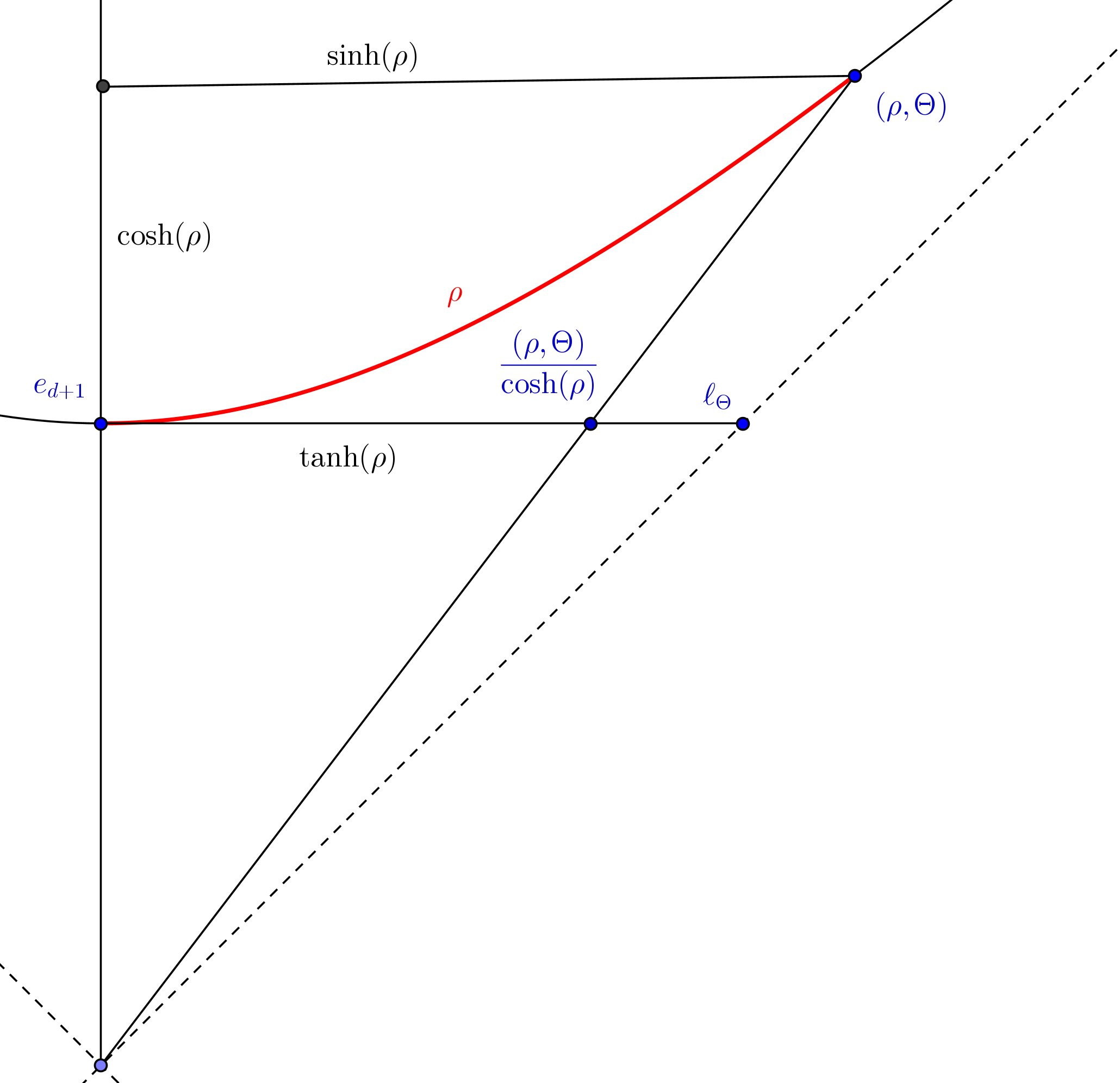
Figure 1: To Lemma 2.22.

Lemma 2.23.

Let $K$ be an F-convex set with support function $h$ and total support function $\tilde{H}$.

• If for any $\Theta$, $h(\eta,\Theta)=o(\cosh(\rho(\eta))),\eta\to\infty$ (in particular if $h$ is bounded) then $\tilde{H}$ equals $0$ on $\partial{\mathcal{F}}$.

• If $\tilde{H}$ equals $0$ on $\partial{\mathcal{F}}$, $h$ is either negative and $K\subset\overline{{\mathcal{F}}}^{\star}$ or $h$ is equal to $0$ and $K=\overline{{\mathcal{F}}}$.

Proof.

If $h$ satisfies the hypothesis, it is immediate from the previous lemma that $\tilde{H}$ equals $0$ on $\partial{\mathcal{F}}$. As $\tilde{H}$ is convex and equal to $0$ on $\partial{\mathcal{F}}$, it is non-positive on ${\mathcal{F}}$. Suppose that there exists $x\in{\mathcal{F}}$ with $\tilde{H}(x)=0$, and let $y\in{\mathcal{F}}\setminus\{x\}$. By homogeneity, $\tilde{H}(\lambda x)=0$ for all $\lambda>0$. Up to choose an appropriate $\lambda$, we can suppose that the line joining $\lambda x$ and $y$ meets $\partial{\mathcal{F}}$ in two points. Let $\ell$ be the one such that there exists $t\in]0,1[$ with $\lambda x=t\ell+(1-t)y$. By convexity and because $\tilde{H}(\lambda x)=\tilde{H}(\ell)=0$, we get $0\leq\tilde{H}(y)$, hence $\tilde{H}(y)=0$ and $H\equiv 0$. The conclusion follows from (13). ∎

Remark 2.24 (Intrinsic properties of restricted support functions).

Let $h$ be the restricted support function of a F-convex set $K$, with homogeneous extension $H$ on ${\mathcal{F}}$.

• $h$ is locally Lipschitz. Actually as a convex function, $H$ is locally Lipschitz for the usual Euclidean metric on ${\mathbb{R}}^{d+1}$. Clearly $h$ is Lipschitz on ${\mathbb{H}}^{d}$ for the Riemannian metric induced by the Euclidean ambient metric. The result follows because local Lipschitz condition does not depend on the Riemannian metric.

• $h$ is $(-1)$-convex. This means that on any unit speed geodesic $\gamma$, there exists a function $f$ such that $f$ is a solution of $f^{\prime\prime}-f=0$, $h\circ\gamma=f$ at a point $t$, and $h\geq f$ near $t$. This is usually denoted by $h^{\prime\prime}-h\geq 0$. In our case, $f$ is given by the restriction of the support function of the future cone of any point of $\partial_{s}K$ contained in a support plane orthogonal to $\gamma(t)\in{\mathbb{H}}^{d}\subset{\mathbb{R}}^{d+1}$.

• Actually any $(-1)$-convex function $h$ on ${\mathbb{H}}^{d}$ is a support function. It suffices to prove that the extension $H$ of $h$ to ${\mathcal{F}}$ is subadditive. Let $x,y\in{\mathcal{F}}$. They span a plane $P$, which defines a geodesic $\gamma$ on ${\mathbb{H}}^{d}$. Let $f$ and $F$ as above, such that $h=f$ at $(x+y)/\|x+y\|_{-}$. Then $H(x+y)=F(x+y)=F(x)+F(y)\leq H(x)+H(y)$.

• A classical example of $(-1)$-convex function on ${\mathbb{H}}^{d}$ is the composition of $\cosh(\cdot)-1$ with the distance to a point $p$. The extension of this function on ${\mathcal{F}}$ is $-\langle p,\cdot\rangle_{-}-\|\cdot\|_{-}$, which is the support function of the convex side of the unit hyperboloid in the future cone at $-p$.

Remark 2.25 (Euclidean support function of F-convex sets).

Let $\eta$ be a support vector of an F-convex set $K$, orthogonal to a support plane $\mathcal{H}$. For a vector $v\in\mathcal{H}$, $\langle v,\eta\rangle_{-}=0$, i.e. in matrix notation, ${}^{t}v.J.\eta=0$, $J=\mathrm{diag}(1,\ldots,1,-1).$ So $v$ is orthogonal to $J\eta$ for the standard Euclidean metric: $J\eta$ is an Euclidean outward support vector to $K$. Hence the Euclidean support function of an F-convex set is defined on the intersection of the Euclidean unit sphere and the interior of the past cone of the origin. Let us denote by $S$ the map from ${\mathbb{H}}^{d}$ to this part of $\mathbb{S}^{d}$:

$$S(\eta)=\frac{J\eta}{\|J\eta\|}=\frac{J\eta}{\|\eta\|},$$

with $\langle\cdot,\cdot\rangle$ the usual scalar product and $\|\cdot\|$ the associated norm. Let $x\in K$ with $h(\eta)=\langle x,\eta\rangle_{-}$. So

$$h(\eta)=\langle x,J\eta\rangle=\langle x,S(\eta)\rangle\|\eta\|,$$

and for suitable radial coordinates on ${\mathbb{H}}^{d}$, $\eta=(0,\ldots,0,\sinh(\rho),\cosh(\rho))$, so if $h^{E}$ is the Euclidean support function of $K$ (the supremum is reached at the same point $x$ for the two bilinear forms):

$$h(\eta)=\sqrt{\cosh(2\rho)}h^{E}(S(\eta)).$$

Remark 2.26 (Restricted support function on the ball).

An extended support function $H$ is also defined by its restriction onto the intersection of any space-like hyperplane with the interior of ${\mathcal{F}}$. This set can be identified with the open ball $B$ of $\mathbb{R}^{d}$. We do not need this here, but this is relevant for example to study the Minkowski problem [BF14]. This reference also consider F-convex sets as graphs on a space-like hyperplane, that we also do not consider here. But let us note for the next remark that restriction of extended support functions on $B$ are exactly convex functions on $B$.

Remark 2.27 (A function not bounded on the boundary).

It is tempting to say that if, for any $\Theta$, $\underset{\rho\rightarrow+\infty}{\mathrm{lim}}\frac{h_{K}(\rho,\Theta)}{\cosh(\rho)}$ is finite, then $K$ is contained in the future cone of a point, taking the supremum for $\Theta$ of the limits. But this is false: there exist convex functions on the closed ball $\overline{B}$ (see the preceding remark), lower-semi continuous and unbounded. They are constructed in Lemma p. 870 of [GKR68]. In this reference there are also constructed convex functions on the closed ball $\overline{B}$, lower-semi continuous, bounded, which attain no maximum.

2.8 Polyhedral sets

Let $p_{i},i\in I$, be a discrete set of points of ${\mathbb{R}}^{d+1}$. Let us suppose that for all $\eta\in{\mathbb{H}}^{d}$, $\operatorname{sup}_{i}\langle\eta,p_{i}\rangle_{-}$ is finite, and moreover that the supremum is attained. That is obviously not always the case, as $-ie_{d+1}$ and $\frac{1}{i}e_{d+1}$ show for $i\in\mathbb{N}$. The function

$$H(\eta)=\operatorname{max}_{i}\langle\eta,p_{i}\rangle_{-}$$

from ${\mathcal{F}}$ to $\mathbb{R}$ is clearly sublinear. From Lemma 2.18 there exists an F-convex set $K$ with support function $H$. We call an F-convex set obtained in this way an F-convex polyhedron. In particular

$$K=\{x\in{\mathbb{R}}^{d+1}|\langle x,\eta\rangle_{-}\leq\operatorname{max}_{i}\langle\eta,p_{i}\rangle_{-}\}.$$

Without loss of generality, we suppose that the set $p_{i},i\in I$ is minimal, in the sense that if a $p_{j}$ is removed from the list, a different F-convex polyhedron is then obtained. In particular, for any $i$ there exists $\eta$ with $H(\eta)=\langle\eta,p_{i}\rangle_{-}$, so $p_{i}\in\partial_{s}K$. Note that by Lemma 2.9, $p_{i}-p_{j}$ is space-like $\forall i,j$. This last property is not a sufficient condition on the $p_{i}$ to define an F-convex polyhedron, as the example $p_{i}=iv$ for any space-like vector $v$ and $i\in\mathbb{N}$ shows.

An F-convex polyhedron can be described more geometrically as a “future convex hull”. If $\mathcal{H}$ is a space-like hyperplane, we denote by $\mathcal{H}^{+}$ its future side.

Lemma 2.28.

Let $K$ be an F-convex polyhedron as above. $K$ is the smallest F-convex set containing the $p_{i}$.

Moreover,

$$K=\cap\{\mathcal{H}^{+}|p_{i}\in\mathcal{H}^{+}\forall i\}.$$

Proof.

Let $K^{\prime}$ be an F-convex set containing the $p_{i}$. For any $\eta\in{\mathcal{F}}$

$$H_{K^{\prime}}(\eta)=\operatorname{sup}_{x\in K^{\prime}}\langle x,\eta\rangle_{-}\geq\langle\eta,p_{i}\rangle_{-}$$

for all $i$ hence

$$H_{K^{\prime}}(\eta)\geq\operatorname{max}_{i}\langle\eta,p_{i}\rangle_{-}=H(\eta)$$

hence $K\subset K^{\prime}$. Let $A=\cap\{\mathcal{H}^{+}|p_{i}\in\mathcal{H}^{+}\forall i\}$. $K$ is an intersection of the future side of space-like hyperplanes (namely its support planes), which all contains the $p_{i}$’s, hence $A\subset K$. By Lemma 2.6, $A$ is an F-convex set, hence $K\subset A$ by the previous property. ∎

Let $K$ be an F-convex polyhedron as above. It gives a decomposition of ${\mathbb{H}}^{d}$ by sets

$$O_{i}=\{\eta\in{\mathbb{H}}^{d}|H(\eta)=\langle\eta,p_{i}\rangle_{-}\}.$$

Lemma 2.29.

The $O_{i}$’s are convex sets and $O_{i}\cap O_{j}$ is contained in a totally geodesic hypersurface if not empty.

Proof.

Let us denote by $C(O_{i})$ the cone over $O_{i}$ in ${\mathcal{F}}$. We have to prove that $C(O_{i})$ is convex in ${\mathbb{R}}^{d+1}$. Let $\eta_{1},\eta_{2}\in C(O_{i})$. Then, for $t\in[0,1]$, as extended support functions are convex,

$$H((1-t)\eta_{1}+t\eta_{2})\leq(1-t)H(\eta_{1})+tH(\eta_{2})=\langle(1-t)\eta_{1}+t\eta_{2},p_{i}\rangle_{-}\leq H((1-t)\eta_{1}+t\eta_{2})$$

hence $H((1-t)\eta_{1}+t\eta_{2})=\langle(1-t)\eta_{1}+t\eta_{2},p_{i}\rangle_{-}$ that means that $(1-t)\eta_{1}+t\eta_{2}\in C(O_{i})$.

For any $\eta\in O_{i}\cap O_{j}$ we get $\langle\eta,p_{i}-p_{j}\rangle_{-}=0$ that is the equation of a time-like vector hyperplane. ∎

A part $F$ of $O_{i}\subset{\mathbb{H}}^{d}$ is a $k$-face, $k=0,\ldots,d$, if $k$ is the smallest integer such that $F$ can be written as an intersection of $(d+1-k)$ $O_{j}$. A $0$-face is a vertex, a $(d-1)$-face is a facet and a $d$ face is a cell $O_{i}$ of the decomposition $\{O_{i}\}$. Let $\eta\in{\mathbb{H}}^{d}$ and $\mathcal{H}$ be the support plane of $K$ with normal $\eta$. If $\eta$ belongs to the interior of a $k$-face $F$, it is easy to see that $\mathcal{H}\cap K$ does not depend on $\eta\in F$ but only on $F$. The set $\mathcal{H}\cap K$ is called a $(d-k)$-face of $K$. As an intersection of convex sets, the faces of $K$ are convex. By construction a $(d-k)$-face contains at least $(d-k+1)$ of the $p_{i}$. As the normal vectors of the hyperplane containing it span a $k+1$ vector space, the $(d-k)$-face is contained in a plane of dimension $(d-k)$, and is not contained in a plane of lower dimension.

A $0$-face is a vertex, a $1$-face is an edge and a $d$-face is a facet of $K$. The vertices are exactly the $p_{i}$. An F-convex polyhedron must have vertices, but maybe no other $k$-faces as the example of the future cone of a point shows.

From Proposition 9.9 and Remark 9.10 in [Bon05], the decomposition given by the $O_{i}$ is locally finite (each $\eta\in{\mathbb{H}}^{d}$ has a neighborhood intersecting a finite number of $O_{i}$). Nevertheless the cells $O_{i}$ can have an infinite number of sides (see Figure 3.6 in [Mar07] where the lift of a simple closed geodesic on a punctured torus is drawn). In this case, the decomposition of $\partial_{s}K$ into faces is not locally finite, for example a vertex can be the endpoint of an infinite number of edges.

We call an F-convex polyhedron $K$ a space-like F-convex polyhedron if the $O_{i}$ are compact convex hyperbolic polyhedra (each with finite number of faces). Each vertex of the decomposition corresponds to a space-like facet of $K$, which is a compact convex polyhedron. Moreover $\partial_{s}K$ is locally finite for the decomposition in facets. It must have an infinite number of faces.

Example 2.30.

Let $x\in{\mathcal{F}}$. Then the convex hull of $\Gamma x$ is a space-like Fuchsian convex polyhedron, because fundamental domains for $\Gamma$ gives a tessellation of ${\mathbb{H}}^{d}$ by compact convex polyhedra [NP91]. A dual construction consists of considering the orbit of a space-like hyperplane [Fil13].

Figure 2: The elementary example in $d=2$.

Let us now consider the case of an F-regular domain $K$. From [Bon05], the image by the Gauss map $G$ of points of $\partial_{s}K$ gives a decomposition of ${\mathbb{H}}^{d}$ by convex sets which are convex hulls of points on $\partial_{\infty}{\mathbb{H}}^{d}$. Of course, if $p\in\partial_{s}K$, the support function $H$ of $K$ is equal to $\langle\cdot,p\rangle_{-}$ on $G(p)$. Hence $K$ is polyhedral in our sense if $K$ has a discrete set of vertices (points $p$ of $\partial_{s}K$ such that $G(p)$ has non empty interior). Following [Bon05], we call them F-regular domains with simplicial singularity.

Example 2.31 (The elementary example).

Figure 2 is an elementary examples of F-regular domains with simplicial singularity. The letters on the F-convex sets are edge-lengths. The letters on the cellulation of ${\mathbb{H}}^{2}$ are measures that will be introduced later. Actually we will call this example (the union the the future cones of points on a space-like segment) “the” elementary example, which is the simplest one, right after the future cone over a point.

2.9 Duality

The notion of duality has interest in its own, but here it will only be used as a tool in the proof of Proposition 2.47. See [Ber14] for a previous introduction. Let $A$ be a set which does not contain the origin. The dual of $A$ is

$$A^{*}=\{x\in{\mathbb{R}}^{d+1}|\langle x,a\rangle_{-}\leq-1,\forall a\in A\}.$$

It is immediate that $A^{*}$ is a closed convex set which does not contain the origin, that $A\subset A^{**}=:(A^{*})^{*}$ and that $A\subset B$ implies $B^{*}\subset A^{*}$, see [Sch93a, 1.6.1]. Note that as an F-convex set contains the future cone of its points, it meets any future time-like ray from the origin.

Lemma 2.32.

Let $K$ be an F-convex set which does not contain the origin. Then $K^{*}$ is contained in $\overline{{\mathcal{F}}}^{\star}$

Proof.

Let $x\notin\overline{{\mathcal{F}}}$. Then there exists a $k\in K$ such that $\langle x,k\rangle_{-}\geq 0$, so $x\notin K^{*}$. As by definition $0\notin K^{*}$, we have $K^{*}\subset\overline{{\mathcal{F}}}^{\star}$. ∎

In the compact case, duality is defined for convex bodies with the origin in their interior, that is equivalent to say that the Euclidean support functions are positive, and we get the fundamental property that the dual of the dual is the identity.

The lemma above says that in our case, even if $0\notin K$, we can take $K\nsubseteq\overline{{\mathcal{F}}}^{\star}$, and then $K^{*}\subset\overline{{\mathcal{F}}}^{\star}$ and $(K^{*})^{*}\subset\overline{{\mathcal{F}}}^{\star}$, so $(K^{*})^{*}\not=K$. Actually the genuine analog to the compact case is that the support function is negative. By (13) this is equivalent to say that $K$ is contained in $\overline{{\mathcal{F}}}^{\star}$.

Lemma 2.33.

Let $K$ be an F-convex set contained in $\overline{{\mathcal{F}}}^{\star}$. Then $K^{*}$ is a F-convex set and $(K^{*})^{*}=K$.

Proof.

$K^{*}$ is a closed convex set, so it is determined by its total support function. For $\eta\in{\mathcal{F}}$ let us consider $\tilde{H}_{K^{*}}(\eta)=\mathrm{sup}\{\langle\eta,x\rangle_{-}\forall x\in K^{*}\}$. There exists $\lambda>0$ such that $\lambda\eta\in K$, so as $\tilde{H}_{K^{*}}(\eta)=\frac{1}{\lambda}\tilde{H}_{K^{*}}(\lambda\eta)$ and by definition $\langle\lambda\eta,x\rangle_{-}\leq-1$ $\forall x\in K^{*}$, $\tilde{H}_{K^{*}}$ has finite values on ${\mathcal{F}}$. As for two future vectors $u,v$ we have $\langle u,v\rangle_{-}<0$ and $K\subset\overline{{\mathcal{F}}}^{\star}$, if $x\in K^{*}$ then $x+\overline{{\mathcal{F}}}\subset K^{*}$, so $\tilde{H}_{{\mathcal{C}}(x)}\leq\tilde{H}_{K^{*}}$, hence $\tilde{H}_{K^{*}}$ is infinite outside of $\overline{{\mathcal{F}}}$. So

$$K^{*}=\{x\in{\mathbb{R}}^{d+1}|\langle x,\eta\rangle_{-}\leq\tilde{H}_{K^{*}}(\eta),\forall\eta\in\overline{{\mathcal{F}}}\}$$

and by Lemma 2.17 we have

$$K^{*}=\{x\in{\mathbb{R}}^{d+1}|\langle x,\eta\rangle_{-}\leq\tilde{H}_{K^{*}}(\eta),\forall\eta\in{\mathcal{F}}\}$$

that says exactly that $K^{*}$ is an F-convex set.

To prove that $(K^{*})^{*}=K$ one has to prove that $(K^{*})^{*}\subset K$. Let $z\notin K$. There exists a support plane of $K$, orthogonal to some $\eta\in{\mathcal{F}}$, which separates $z$ from $K$ [Sch93a, 1.3.4]. Hence there exists $\alpha$ with $\langle z,\eta\rangle_{-}>\alpha$ and $\langle k,\eta\rangle_{-}<\alpha$ for all $k\in K$. From (13), $\alpha<0$. On the other hand, for any $k\in K$, $\langle k,\eta\rangle_{-}\leq\alpha$, which can be written $\langle k,\frac{\eta}{-\alpha}\rangle_{-}\leq-1$, hence $\frac{\eta}{-\alpha}\in K^{*}$. But $\langle z,\frac{\eta}{-\alpha}\rangle_{-}>-1$, so $z\notin(K^{*})^{*}$. ∎

Let $K$ be an F-convex contained in $\overline{{\mathcal{F}}}^{\star}$. The radial function of $K$ is the function from $\overline{{\mathcal{F}}}^{\star}$ to ${\mathbb{R}}^{+}\cup\{+\infty\}$ defined by

$$R_{K}(\eta):=\mathrm{inf}\{s>0|s\eta\in K\}.$$

$R_{K}$ has always finite values on ${\mathcal{F}}$. If $K$ does not meet the light-like ray directed by $\ell$, then $R_{K}(\ell)=+\infty$. In particular $\forall\eta$, $R_{K}(\eta)\eta\in\partial K$, $R_{K}$ is homogeneous of degree $-1$ and

$$K=\{\eta\in\overline{{\mathcal{F}}}^{\star}|R_{K}(\eta)\leq 1\}.$$

Lemma 2.34.

Let $K$ be an F-convex set contained in $\overline{{\mathcal{F}}}^{\star}$. Then on $\overline{{\mathcal{F}}}^{\star}$, the total support function $\tilde{H}_{K^{*}}$ of $K^{*}$ satisfies

$$\tilde{H}_{K^{*}}=\frac{-1}{R_{K}}.$$

As $K\subset\overline{{\mathcal{F}}}^{\star}$, $\tilde{H}_{K^{*}}$ and $\tilde{H}_{K}$ have finite non-positive values on $\overline{{\mathcal{F}}}$.

Proof.

We define $X=\{x\in\overline{{\mathcal{F}}}^{\star}|\tilde{H}_{K^{*}}(x)\leq-1\}.$ Let us first prove that $K=X$.

Let $x\in K\cap{\mathcal{F}}$. There exists $v\in K^{*}$ such that $\tilde{H}_{K^{*}}(x)=\langle v,x\rangle_{-}$. But by definition of $K^{*}$, $\langle v,x\rangle_{-}\leq-1$ hence $x\in X$. If $K\cap\partial{\mathcal{F}}$ is empty, we have $K\subset X$. If not, for $x\in K\cap\partial{\mathcal{F}}$ the result is obtained from the previous case using Lemma 2.17.

Let $x\in X$. By definition of the support function, for any $v\in K^{*}$ we have $\langle x,v\rangle_{-}\leq\tilde{H}_{K^{*}}(x)$. On the other hand, as $x\in X$, $\tilde{H}_{K^{*}}(x)\leq-1$ hence $x\in(K^{*})^{*}=K$. We proved that $K=X$.

Let us suppose that there exists $x$ with $\tilde{H}_{K^{*}}(x)>\frac{-1}{R_{K}(x)}$. As $\tilde{H}_{K^{*}}$ and $\frac{-1}{R_{K}}$ are $1$-homogeneous, one can find $\lambda>0$ such that $\tilde{H}_{K^{*}}(\lambda x)>-1>\frac{-1}{R_{K}(\lambda x)}$. So $\lambda x\in K\setminus X$, that is impossible. ∎

Example 2.35.

Let $p\in\overline{{\mathcal{F}}}^{\star}$. Then ${\mathcal{C}}(p)^{*}$ is the intersection of $\overline{{\mathcal{F}}}$ with the half-space $\{\langle x,p\rangle_{-}\leq-1\}$.

The dual of $K({\mathbb{H}}_{t})$ is $K({\mathbb{H}}_{1/t})$. More striking is the dual of $K({\mathbb{H}})+{\mathcal{C}}(e_{d+1})$. It is not hard to see that on ${\mathbb{H}}^{d}$, $R_{K({\mathbb{H}})+{\mathcal{C}}(e_{d+1})}(\eta)=2\eta_{d+1}$, so $H_{(K({\mathbb{H}})+{\mathcal{C}}(e_{d+1}))^{*}}(\eta)=\langle\eta,\eta\rangle_{-}/(-2\langle e_{d+1},\eta\rangle_{-})$, see Figure 3. Note that on $\partial{\mathcal{F}}^{\star}$, $R_{(K({\mathbb{H}})+{\mathcal{C}}(e_{d+1}))^{*}}=1$. So $K\subset{\mathcal{F}}^{\star}$ does not imply $K^{*}\subset{\mathcal{F}}^{\star}$.

Example 2.36.

The dual of a $\Gamma$ invariant F-convex set is a $\Gamma$ invariant F-convex set.

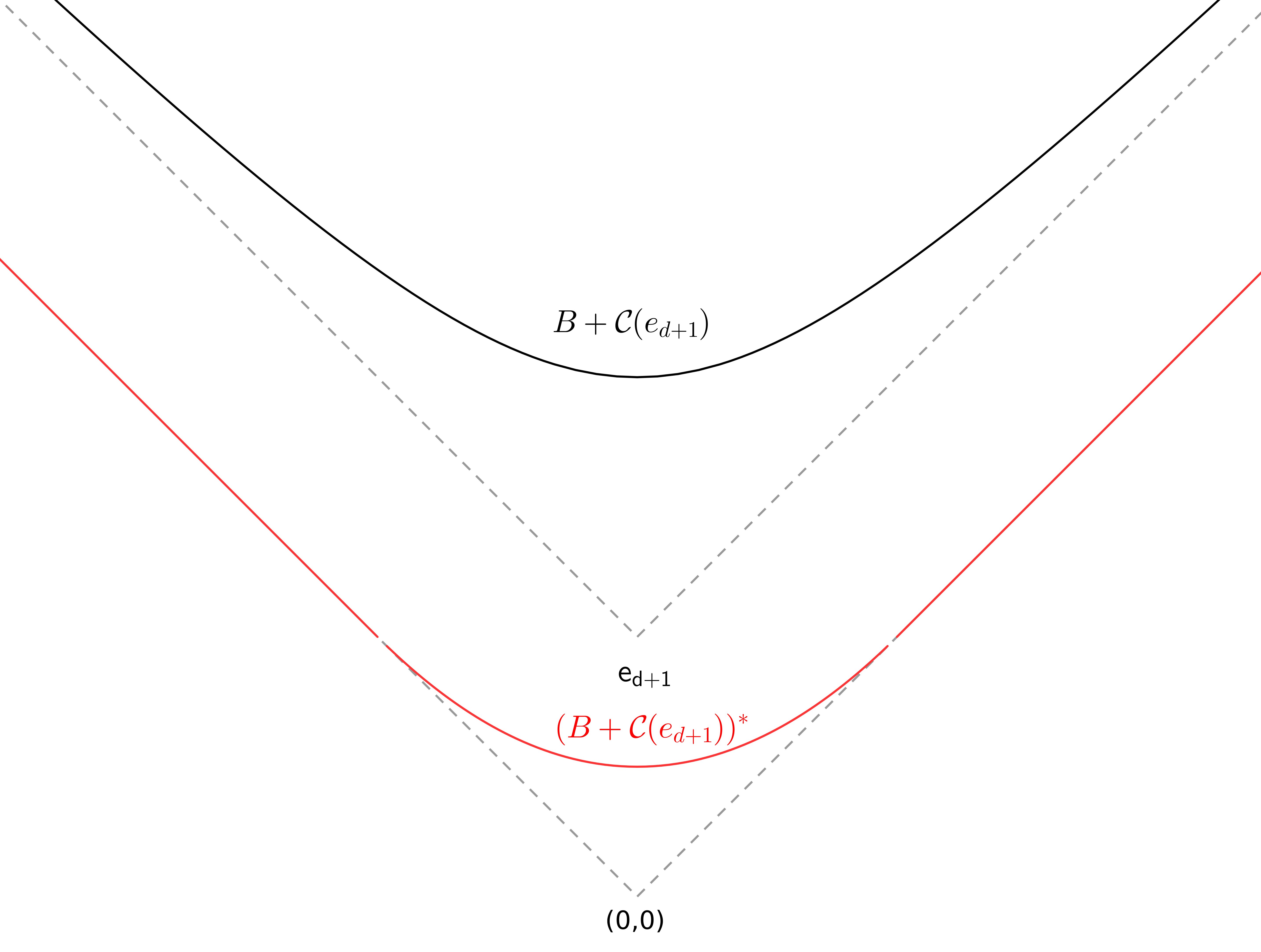
Figure 3: $K({\mathbb{H}})+{\mathcal{C}}(e_{d+1})$ and its dual.

2.10 First order regularity

Lemma 2.37.

Let $\eta\in{\mathcal{F}}$, $K$ be an F-convex set and $\mathcal{H}$ be the space-like support plane of $K$ with normal $\eta$. The intersection of $K$ and $\mathcal{H}$ is reduced to one point $p$ if and only if $H$ is differentiable at $\eta$. In this case $p$ is equal to the gradient $\mathrm{grad}_{\eta}H$ (for $\langle\cdot,\cdot\rangle_{-}$) of $H$ at $\eta$.

This result is a classical fact for convex bodies in the Euclidean space [Sch93a], and the adaptation of the proof is straightforward. See [Fil13], where this property is checked for Fuchsian convex sets, but the group invariance does not enter the proof.

An F-convex set is said to be $C^{k}$ if $\partial_{s}K$ is a $C^{k}$ submanifold of ${\mathbb{R}}^{d+1}$.

Lemma 2.38.

Let $K$ be an F-convex set with support function $h_{K}$ and extended support function $H_{K}$.

1. $K$ is $C^{1}$ if and only if it has a unique support plane at each boundary point.

2. If there exist $\eta,\eta^{\prime}\in{\mathcal{F}}$ with $H_{K}(\eta+\eta^{\prime})=H_{K}(\eta)+H_{K}(\eta^{\prime})$ then there exists $k\in K$ with two support planes. In particular $K$ is not $C^{1}$.

3. $h_{K}$ is $C^{1}$ if and only if $\partial_{s}K$ is strictly convex (i.e. the intersection of $K$ with any space-like support plane is reduced to a point).

4. If $K$ is strictly convex, then $h_{K}$ is $C^{1}$ and $\partial_{s}K=\partial K$.

5. If $h_{K}$ is $C^{1}$ and $\partial_{s}K=\partial K$, then $K$ is strictly convex.

6. If $K$ is $C^{1}$ then the Gauss map is a well defined continuous map. If $\partial_{s}K$ is strictly convex, then the Gauss map has a well defined inverse.

It follows that if $\partial_{s}K$ is $C^{1}$ and strictly convex, the Gauss map is a continuous bijection (it is surjective by assumption). We will see in Subsection 2.12 that in this case it is actually a homeomorphism.

Proof.

(i) is a general property of closed convex sets, see [Sch93a] p. 104. Suppose that the hypothesis of (ii) holds. Let $k,x,x^{\prime}$ be points of $K$ with respectively $\langle k,\eta+\eta^{\prime}\rangle_{-}=H_{K}(\eta+\eta^{\prime})$, $\langle x,\eta\rangle_{-}=H_{K}(\eta)$, $\langle x^{\prime},\eta^{\prime}\rangle_{-}=H_{K}(\eta^{\prime})$. By assumption we get $\langle k,\eta\rangle_{-}=\langle x,\eta\rangle_{-}+\langle x^{\prime}-k,\eta^{\prime}\rangle_{-}$, and $\langle x^{\prime}-k,\eta^{\prime}\rangle_{-}\geq 0$ so $\langle k,\eta\rangle_{-}\geq\langle x,\eta\rangle_{-}=H_{K}(\eta)$, so $H_{K}(\eta)=\langle k,\eta\rangle_{-}$, that means that the support plane directed by $\eta$ contains $k$, which is also in the support plane directed by $\eta+\eta^{\prime}$. By (i) $K$ is not $C^{1}$.

From Lemma 2.37 the intersection of $K$ with any of its space-like support planes is reduced to a point if and only if $H_{K}$ is differentiable, that occurs if and only if $H_{K}$ is $C^{1}$, as $H_{K}$ is convex (see e.g. [HUL93, p. 189]). This is (iii), that implies (v). (iv) follows because if $K$ is strictly convex it has only space-like support planes due to (iv) of Lemma 2.5.

From (i), the Gauss map is well defined if $K$ is $C^{1}$. In this case, the volume form of $\partial_{s}K$ is continuous, and, by the identification induced by $\langle\cdot,\cdot\rangle_{-}$ between $d$-forms and vectors on $\mathbb{R}^{d+1}$, normal vectors to $\partial_{s}K$ are continuous.

If $K$ is strictly convex, the inverse of the Gauss map is clearly well defined. ∎

Example 2.39.

If $H$ is the extended support function of ${\mathcal{C}}(p)$, it is immediate that $\mathrm{grad}_{\eta}H=p,\forall\eta\in{\mathcal{F}}$. It is important to not confuse $\partial_{s}{\mathcal{C}}(p)$ (the single point $p$) and $\partial{\mathcal{C}}(p)$ (the boundary of the cone), as $H$ is $C^{1}$ but ${\mathcal{C}}(p)$ is not strictly convex.

2.11 Orthogonal projection

Let $K$ be an F-convex set. We recall some facts which are contained in [Bon05], especially Proposition 4.3. For any point $k\in K$, there exists a unique point $r(k)$ on $\partial K$ which is contained in the closure of the past cone of $k$ and which maximizes the Lorentzian distance. The hyperplane orthogonal to $(k-r(k))$ is a support plane of $K$ at $r(k)$. In particular $r(K)=\partial_{s}K.$ The map $k\mapsto r(k)$ is the Lorentzian analogue of the Euclidean orthogonal projection onto a convex set, see Figure 4. The cosmological time of $K$ is $T(k)=d_{L}(k,r(k))$ for any $k\in K$. This is the analogue of the distance between a point and a convex set in the Euclidean space.

The normal field of $K$ is the map $N:K\setminus\partial K\rightarrow{\mathbb{H}}^{d}$ defined by $N(k)=\frac{1}{T(k)}(k-r(k))$. The normal field is well-defined and continuous, because equal to minus the Lorentzian gradient of $T$, and $T$ is a $C^{1}$ submersion on the interior of $K$. $N$ is surjective by definition of F-convex set. Note that $\|\operatorname{grad}T\|_{-}=1$.

\begin{picture}(3678.0,1544.0)(2590.0,-2048.0)\end{picture}

Figure 4: For the Euclidean metric, orthogonal projection onto a convex set is well-defined. For the Lorentzian metric, orthogonal projection onto the complementary of a space-like convex set is well-defined.

Let $\omega$ be a Borel set of ${\mathbb{H}}^{d}$ and $I$ be a non-empty interval of positive numbers (maybe reduced to a point). We introduce the following sets, see Figure 5:

$$K_{I}=T^{-1}(I),$$

$$K_{I}(\omega)=K_{I}\cap N^{-1}(\omega),$$

$$K(\omega)=G^{-1}_{K}(\omega).$$

We have some immediate properties:

• $K_{t}$ is the boundary of the F-convex set $K+tK({\mathbb{H}})$. If $h$ is the support function of $K$ and $H$ is its $1$-extension, then the support function of $K_{t}$ is $h-t$ and its extended support function is $H-t\|\cdot\|_{-}$. It follows easily that $K$ and $K_{t}$ have the same light-like support planes at infinity. Finally, $K_{t}$ has no light-like support plane.

• For $t>0$, the restriction of the normal field to $K_{t}=T^{-1}(t)$ is equal to the Gauss map $G_{K_{t}}$ of $K_{t}$. In particular, $K_{t}(\omega)=G^{-1}_{K_{t}}(\omega)$ and $\partial K_{t}$ is a $C^{1}$ space-like hypersurface (it is actually $C^{1,1}$ [Bar05, 4.12]).

• The restriction of the normal field to $K_{t}$ is a proper map [Bon05, 4.15] (as $K_{t}$ is $C^{1}$, the Gauss map is well-defined). Hence, if $\omega\subset{\mathbb{H}}^{d}$ is compact, $K_{t}(\omega)$ is compact.

• The map $r:K\rightarrow\partial_{s}K$ is continuous [Bon05, 4.3].

• If $\omega\subset{\mathbb{H}}^{d}$ is compact then $K(\omega)$ is compact, by the two previous items and because $r(K_{t}(\omega))=K(\omega)$.

This allows to prove that $\partial_{s}K$ determines $K$ in the following sense.

Lemma 2.40.

Let $K$ be an F-convex set. Then

$$K=\bigcup_{k\in\partial_{s}K}\mathcal{C}(k).$$

Proof.

Because of (i) of Lemma 2.5, $\bigcup_{k\in\partial_{s}K}\mathcal{C}(k)\subset K.$ Because $r(K)=\partial_{s}K$, for any $p\in K$ there exists $k\in\partial_{s}K$ such that $p\in\mathcal{C}(k)$. ∎

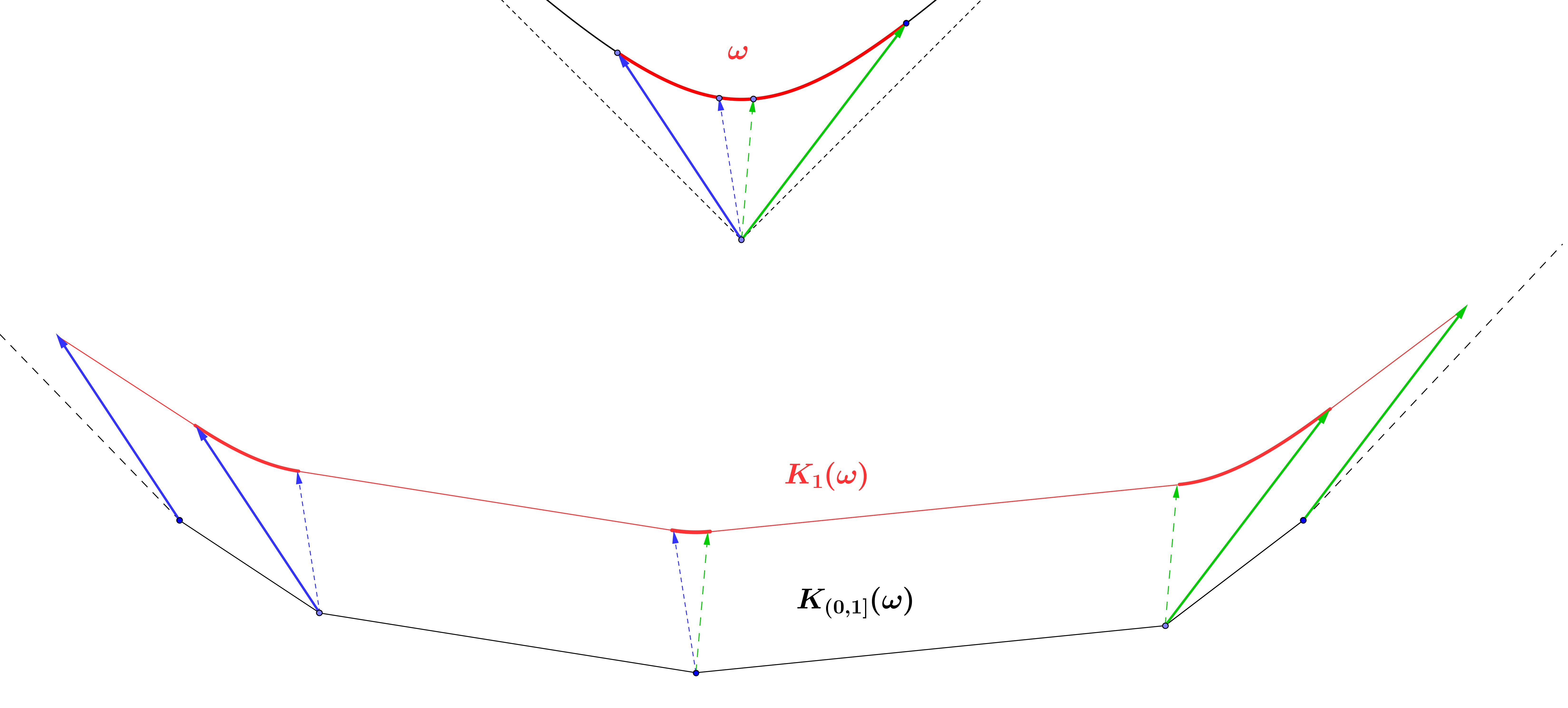
Figure 5: Notations, see Subsection 2.11.

Remark 2.41.

A property of F-convex sets is that the restriction of the normal field to $K_{t}$ is a proper map. Consider as $K$ the future of a line (an angle formed by the future of two light-like planes) in ${\mathbb{R}}^{3}$. The image of the Gauss map is a line $l$ in ${\mathbb{H}}^{2}$. The pre-image of any compact segment of $l$ by the Gauss map of any $K_{t}$ is not bounded.

Remark 2.42.

Let $K$ be a $\tau$-convex set. It is easy to see [Bon05, 4.10] that, if $\gamma\in\Gamma_{\tau}$, with linear part $\gamma_{0}$, then $r\circ\gamma=\gamma\circ r$, $N\circ\gamma=\gamma_{0}\circ N$, hence $T\circ\gamma=T$. It follows that

$$\gamma K_{(0,\varepsilon]}(\omega)=K_{(0,\varepsilon]}(\gamma_{0}\omega).$$

Lemma 2.43.

Let $\tau$ be a cocycle and let $h_{\tau}$ be the support function of $\overline{\Omega_{\tau}}$ (see Example 2.11).

1. An F-convex set $K$ which is (setwise) invariant for the action of $\Gamma_{\tau}$ is contained in $\overline{\Omega_{\tau}}$.

2. All $\tau$-F-convex sets have the same light-like support planes at infinity than $\overline{\Omega_{\tau}}$.

3. A $\tau$-F-convex set contained in $\Omega_{\tau}$ has only space-like support planes.

4. Let $K$ be a $\tau$-F-convex set. If $K\cap\partial\Omega_{\tau}\not=\emptyset$, then $K\cap\partial_{s}\Omega_{\tau}\not=\emptyset$.

5. Let $h$ be the support function of a $\tau$-F-convex set $K$. If $h<h_{\tau}$, then $K\subset\Omega_{\tau}$.

Proof.

Let $K$ as in (i) with extended support function $H$, and let $H_{\tau}$ be the extended support function of $\overline{\Omega_{\tau}}$. As $H-H_{\tau}$ is $0$-equivariant, its restriction to ${\mathbb{H}}^{d}$ reaches a minimum $a$ and a maximum $b$. Hence $H_{\tau}+a\|\cdot\|_{-}\leq H\leq H_{\tau}+b\|\cdot\|_{-}$, so clearly $H$ and $H_{\tau}$ have the same limit on any path $\ell+t(\eta-\ell)$. From Lemma 2.17, both sets have the same light-like support planes at infinity. (This proves (ii) if $K$ is a $\tau$-convex set.) In particular $K$ is contained in the intersection of the future side of those planes, but this intersection is precisely $\Omega_{\tau}$ [Bon05, Corollary 3.7], so $K\subset\overline{\Omega_{\tau}}$.

(iii) We know from Lemma 2.5 that $K$ has no time-like support plane. Let us suppose that $K$ has a light-like support plane $L$, and let $x\in K\cap L$. Then by (ii) $L$ is a support plane at infinity of $\Omega_{\tau}$, but $x\in\Omega_{\tau}$ so $L$ is a support plane of $\overline{\Omega_{\tau}}$. In particular, $x\in\partial\Omega_{\tau}$, that is impossible as $K$ is supposed to be in $\Omega_{\tau}$, which is open.

(iv) Suppose that $K\cap\partial_{s}\Omega_{\tau}=\emptyset$. By cocompactness, $H_{\tau}-H$ (the extended support functions of $\overline{\Omega_{\tau}}$ and $K$) is bounded from below by a positive constant $c$. So $S_{c/2}$, the level set of the cosmological time of $\Omega_{\tau}$ for the value $c/2$, contains $K$. But $S_{c/2}$ has no light-like support plane, so by (ii), $S_{c/2}\cap\partial\Omega_{\tau}=\emptyset$, hence $K\cap\partial\Omega_{\tau}=\emptyset$.

(v) If $h<h_{\tau}$, then $K\cap\partial_{s}\Omega_{\tau}=\emptyset$ and the result follows from (iv). ∎

Remark 2.44.

Lemma 2.18 and Lemma 2.43 imply that there exists a $\tau$-equivariant convex function $H_{\tau}$ such that, for any $\tau$-equivariant convex function $H$, then $H\leq H_{\tau}$.

Example 2.45.

Let $h$ be the support function of a $\Gamma$ invariant F-convex set $K$. Lemma 2.43 says that $K\subset\overline{{\mathcal{F}}}$. Suppose that $K\not=\overline{{\mathcal{F}}}$. From Lemma 2.23, $K\subset\overline{{\mathcal{F}}}^{\star}$, and by Lemma 2.43, $K\subset{\mathcal{F}}$.

2.12 The normal representation

Let $\mathcal{O}$ be an open set of ${\mathbb{H}}^{d}$ and let $h:\mathcal{O}\rightarrow{\mathbb{R}}$ be a $C^{1}$ map with $1$-extension $H$. We call normal representation of $h$ the map $\chi$ from $\mathcal{O}\rightarrow{\mathbb{R}}^{d+1}$ defined by $\chi(\eta)=\mathrm{grad}_{\eta}H$, that is, for any space-like vector $v$,

$$\langle\chi(\eta),v\rangle_{-}=D_{\eta}H(v)$$ (19)

and by Euler’s Homogeneous Function Theorem

$$\langle\chi(\eta),\eta\rangle_{-}=H(\eta).$$ (20)

The equation above defines a space-like hyperplane with normal $\eta$ containing the point $\chi(\eta)$. Lemma 2.37 says that if $H$ is the support function of an F-convex set $K$, then $\chi({\mathbb{H}}^{d})=\partial_{s}K$. If an F-convex set $K$ is $C^{1}$ and $\partial_{s}K$ is strictly convex, we know from Lemma 2.38 that the Gauss map is a continuous bijection. But from (iii) its support function has normal representation, which is clearly the inverse of the Gauss map, which is then a homeomorphism.

Now let $h:\mathcal{O}\rightarrow{\mathbb{R}}$ be $C^{2}$. Then $\chi$ is $C^{1}$. Differentiating (20) in the direction of a space-like vector $v$, and using (19), we get that $\langle\eta,D_{\eta}\chi(v)\rangle_{-}=0$, so if $\eta$ is a regular point, the space-like hyperplane $\langle\cdot,\eta\rangle_{-}=H(\eta)$ is tangent to $\chi(\mathcal{O})$ at $\chi(\eta)$. The differential $S^{-1}$ of $\chi$ is called the reverse shape operator, because $\chi$ is the inverse of the Gauss map, and the differential of the Gauss map is the shape operator. $S^{-1}$ is considered as an endomorphism of $T_{\eta}{\mathbb{H}}^{d}$, by identifying this space with the support plane of $\chi(\eta)$ with normal $\eta$. This allows to define the reverse second fundamental form of $H$: $\forall X,Y\in T_{\eta}{\mathbb{H}}^{d}$,

$$\textsc{II}^{-1}(X,Y):=\langle S^{-1}(X),Y\rangle_{-}=\operatorname{Hess}_{\eta}H(X,Y)\stackrel{{\scriptstyle\eqref{eq:II-1}}}{{=}}\nabla^{2}h(X,Y)-hg(X,Y).$$ (21)

As $\textsc{II}^{-1}(X,Y)=\mathrm{Hess}_{\eta}H_{K}(X,Y)$, $\textsc{II}^{-1}$ is symmetric and the eigenvalues $r_{1},\ldots,r_{d}$ of $S^{-1}$ are real. They are the principal radii of curvature of $h$. If they are not zero, the Gauss map is a $C^{1}$ diffeomorphism, and then the $r_{i}$ are the inverse of the principal curvatures of the space-like hypersurface $\chi(\mathcal{O})$.

2.13 Second order regularity

An F-convex set $K$ is called $C^{2}_{+}$ if $\partial_{s}K$ is $C^{2}$ and its Gauss map is a $C^{1}$ diffeomorphism. This implies that $\partial_{s}K$ is strictly convex, but $K$ is not necessarily strictly convex, as can be seen on Figure 3.

Lemma 2.46.

1. If $h_{K}$ is $C^{2}$, then the radii of curvature are real non-negative numbers.

2. If a $C^{2}$ function $h$ on ${\mathbb{H}}^{d}$ satisfies

   $$(\nabla^{2}h-hg)\geq 0.$$ (22)

   then it is the support function of an F-convex set.

3. If $K$ is $C^{2}_{+}$ then $h_{K}$ is $C^{2}$, the radii of curvature are positive (hence equal to the inverses of the principal curvatures).

Proof.

We already know that the eigenvalues of $S^{-1}$ are real. As $H_{K}$ is convex, its Hessian is positive semidefinite, so (i) holds.

Let $h$ be a function as in (ii). Then its one homogeneous extension to ${\mathbb{R}}^{d+1}$ has a positive semidefinite Hessian, and (ii) follows by Lemma 2.18.

Let us prove (iii). If the Gauss map $G$ is a $C^{1}$ diffeomorphism, its inverse is the normal representation $\chi$, which is then $C^{1}$. As $\chi$ is the gradient of $H_{K}$, $H_{K}$ is $C^{2}$. Moreover the shape operator (the differential of the Gauss map) is the inverse of the reverse shape operator, and both are positive definite, because they are both positive semidefinite and invertible.

∎

Proposition 2.47.

Let $K$ be an F-convex set with support function $h_{K}$. If $h_{K}$ is $C^{2}$ and the principal radii of curvature are positive, i.e. $(\nabla^{2}h_{K}-h_{K}g)>0$, then $K$ is $C^{2}_{+}$.

This proof of this proposition is the content of the next subsection.

Corollary 2.48.

Let $K$ be an F-convex set with support function $h_{K}$.

1. If a $C^{2}$ function $h$ on ${\mathbb{H}}^{d}$ satisfies

   $$(\nabla^{2}h-hg)>0.$$ (23)

   then it is the support function of a $C^{2}_{+}$ F-convex set.

2. If $h_{K}$ is $C^{2}$, then for any $\varepsilon>0$, $K+\varepsilon K({\mathbb{H}})$ is $C^{2}_{+}$.

Proof.

(1) follows from Proposition 2.47 and (ii) of Lemma 2.46. Let $h_{K}$ be $C^{2}$. Then $(\nabla^{2}h-hg)\geq 0$, and for any $\varepsilon>0$, the support function of $K+\varepsilon K({\mathbb{H}})$ is $h_{K}-\varepsilon$ and $(\nabla^{2}(h-\varepsilon)-(h-\varepsilon)g)>0$, and (2) follows from (1)

∎

Remark 2.49.

Let $h$ be a $C^{2}$ function on ${\mathbb{H}}^{d}$ such that $(\nabla^{2}h-hg)\leq 0$, with $1$-extension $H$. Then by the proposition above, $-H$ is the extended support function of an F-convex set $K$, and $\mathrm{grad}(-H)=-\mathrm{grad}H$ is the normal representation of $\partial_{s}K$. Hence $\mathrm{grad}H$ is the normal representation of $\partial_{s}(-K)$, and $-K$ is a P-convex set, see Remark 2.10.

Example 2.50.

The future cone of a point is at the same time an F-convex polyhedron and an F-convex set with $C^{2}$ support function. This is the only case where it can happen.

Example 2.51 (F-convex sets not contained in the future cone of a point).

Let us define, for $x\in{\mathbb{H}}^{d}$, $\rho=\rho(x)$ the hyperbolic distance to $e_{d+1}$, and

$$F_{\alpha}^{+}(x)=\cosh(\rho)^{\alpha},\alpha\geq 1,F_{\alpha}^{-}(x)=-\cosh(\rho)^{\alpha},-1\leq\alpha\leq 1$$

whose degree one extensions on ${\mathcal{F}}$ are respectively

$$\frac{x_{d+1}^{\alpha}}{(-\langle x,x\rangle_{-})^{(\alpha-1)/2}},-\frac{x_{d+1}^{\alpha}}{(-\langle x,x\rangle_{-})^{(\alpha-1)/2}}.$$

As $\cosh\rho$ is the restriction to ${\mathbb{H}}^{d}$ of the map $x\mapsto x_{d+1}$, using (3) and the fact that for $f:\mathbb{R}\rightarrow\mathbb{R}$ one has $\nabla^{2}(f\circ\rho)=(f^{\prime}\circ\rho)\nabla^{2}\rho+(f^{\prime\prime}\circ\rho)\mathrm{d}\rho\otimes\mathrm{d}\rho$, we compute easily that

$$\nabla^{2}\rho=\frac{\cosh\rho}{\sinh\rho}\left(g-\mathrm{d}\rho\otimes\mathrm{d}\rho\right)$$ (24)

and finally

$$\nabla^{2}\cosh^{\alpha}\rho=[\alpha\cosh^{\alpha}\rho]g+[\alpha(\alpha-1)\cosh^{\alpha-2}\rho\ \sinh^{2}\rho]\mathrm{d}\rho\otimes\mathrm{d}\rho.$$ (25)

It follows that $(\nabla^{2}-g)(F^{+}_{\alpha})$ and $(\nabla^{2}-g)(F^{-}_{\alpha})$ are semi-positive definite, hence $F_{\alpha}^{+}$ and $F_{\alpha}^{-}$ are support functions of F-convex sets. Note that $F^{-}_{0}$ is the support function of $K({\mathbb{H}})$, and $F^{-}_{1}$ and $F^{+}_{1}$ are support functions of the future cones of $e_{d+1}$ and $-e_{d+1}$ respectively. From Lemma 2.22, for $\alpha>1$, $F^{+}_{\alpha}$ has no light-like support plane at infinity. See Figure 6.

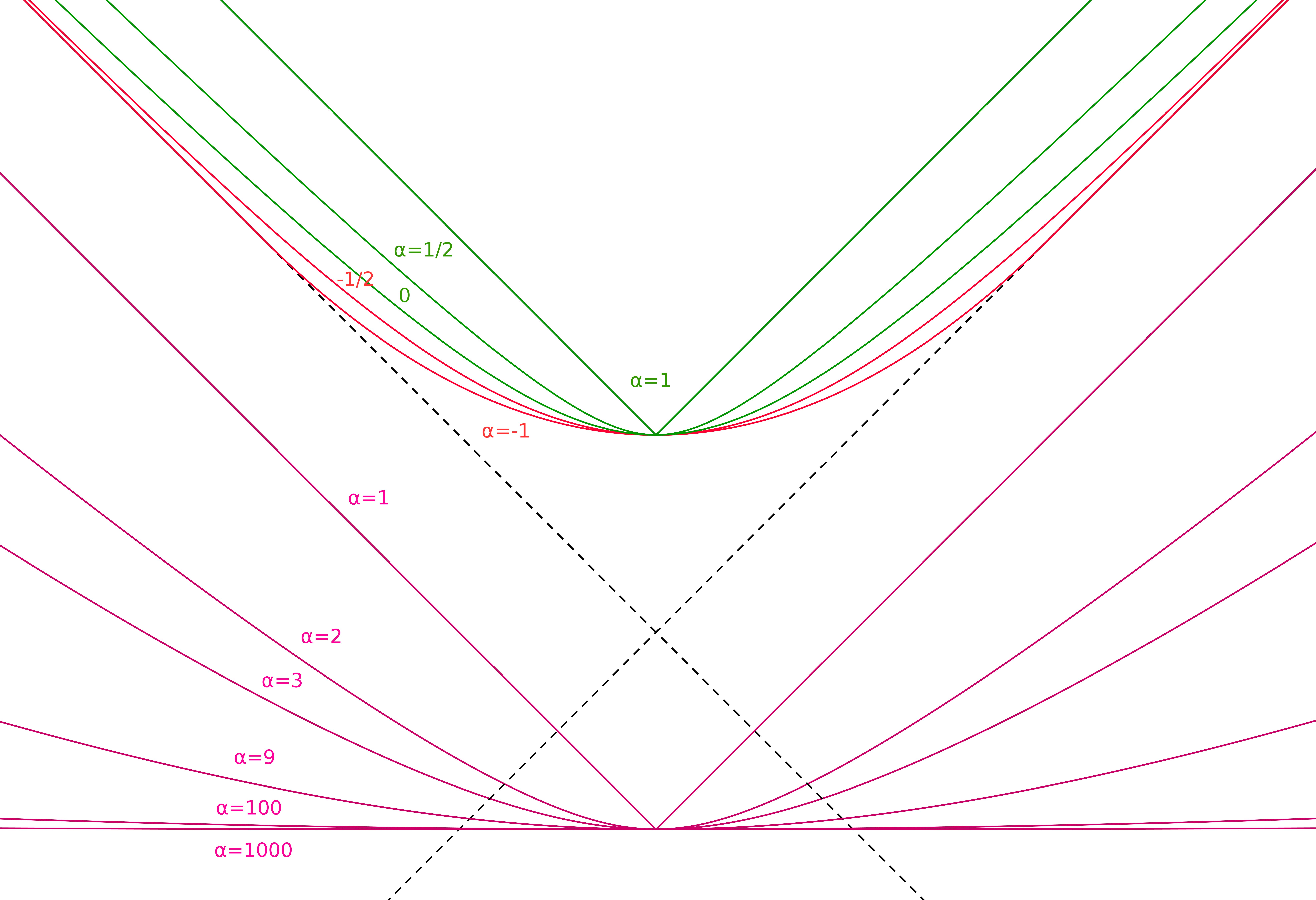
Figure 6: To Example 2.51.

2.14 Proof of Proposition 2.47

As $h_{K}$ is $C^{2}$, $H_{K}$ is $C^{2}$, the normal representation is $C^{1}$, and this is a regular map as the principal radii of curvature (the eigenvalues of its differential) are positive, so $\partial_{s}K$ is $C^{1}$. Moreover as the Gauss map is the inverse of the normal representation, it is a $C^{1}$ diffeomorphism. It remains to prove the non-trivial result that $\partial_{s}K$ is actually $C^{2}$.

First suppose that $K$ is contained in the future cone of a point. Up to a translation, we can consider that this is the future cone of the origin. From Lemma 2.34 and the properties of $H_{K}$, $K^{*}$ is $C^{2}$. At the point $R_{K^{*}}(\eta)\eta$ of the boundary of $K^{*}$, the Gauss map is $\chi(\eta)/(\sqrt{-\langle\eta,\eta\rangle_{-}})$, so a $C^{1}$ diffeomorphism, and then $K^{*}$ is $C^{2}_{+}$. By (iii) of Lemma 2.46, $h_{K^{*}}$ is $C^{2}$ and its principal radii of curvatures are positive. Repeating the argument, we get that $K=(K^{*})^{*}$ is $C^{2}$.

Now suppose that $K$ is not contained in any future cone of a point. We will need the following:

Fact: For any $k\in\partial_{s}K$, there exists a neighborhood $V$ of $k$ in $\partial_{s}K$ and an F-convex set $K_{V}$ such that: $V$ is a part of the boundary of $K_{V}$, $K_{V}$ is contained in the future cone of a point, has $C^{2}$ support function and positive principal radii of curvature.

From the preceding argument, it will follow that the boundary of $K_{V}$ is $C^{2}$, hence each point of $\partial_{s}K$ has a $C^{2}$ neighborhood, hence $K$ is $C^{2}$. Let us prove the fact. We need the following local approximation result.

Lemma 2.52.

Let $K$ be an F-convex set with support function $h_{K}$, $\omega\subset{\mathbb{H}}^{d}$ be compact and $\varepsilon>0$. Then there exists an F-convex set $A(K,\omega,\varepsilon)=:A$ with support function $h_{A}$ such that

• $A$ is $C^{2}_{+}$,

• $\mathrm{sup}_{\eta\in\omega}|h_{K}(\eta)-h_{A}(\eta)|<\varepsilon,$

• $A$ is contained in the future cone of a point.

Proof of Lemma 2.52.

The argument is an adaptation of [Fir74]. The intersection of $K_{\varepsilon/4}(\omega)$ with $\bigcup_{k\in\partial_{s}K}{\mathcal{C}}(k)$ is an open covering of the compact set $K_{\varepsilon/4}(\omega)$ (see Subsection 2.11). From it we get a finite covering $\bigcup_{i=1}^{N}{\mathcal{C}}(k_{i})$. Let $E$ be the convex hull of $\cup_{i}{\mathcal{C}}(k_{i})$. It has extended support function $H_{E}(x)=\mbox{max}_{i=1\cdots N}\langle x,k_{i}\rangle_{-}$, and is an F-convex set due to Lemma 2.18. As $k_{i}\in K$, ${\mathcal{C}}(k_{i})\subset K$ hence $E\subset K$ and $H_{E}\leq H_{K}$ on $\omega$. By construction $K_{\varepsilon/4}(\omega)\subset E$ hence $H_{K}-\varepsilon/4\leq H_{E}$ on $\omega$, and finally $\mbox{sup}_{x\in\omega}|H_{K}(x)-H_{E}(x)|<\varepsilon/3$.

The statement of the lemma and the computation above are true up to translations. We imply that we performed a translation such that $k_{1},\ldots,k_{N}$ are contained in the past cone of the origin, so $\langle x,k_{i}\rangle_{-}>0$ for all $x\in{\mathcal{F}}$. The functions

$$H_{p}(x)=\left(\sum_{i=1}^{N}\langle x,k_{i}\rangle_{-}^{p}/N\right)^{\frac{1}{p}}$$

are extended support functions of F-convex sets by Minkowski inequality and Lemma 2.18. $H_{p}$ is clearly $C^{2}$ (actually analytical), and $H_{p}(x)$ converges to $H_{E}(x)$ when $p\rightarrow\infty$. Let us choose $p=p_{\varepsilon}$ such that $\mbox{sup}_{x\in\omega}|H_{p}(x)-H_{E}(x)|<\varepsilon/3$. From Lemma 2.17, the extension $\tilde{H}_{p}$ of $H_{p}$ to $\partial{\mathcal{F}}$ is a continuous function with finite values. Let ${\mathcal{F}}(1)$ be the subset of $\overline{{\mathcal{F}}}$ made of vectors with last coordinate equal to one. It is a compact set and let $M$ be the maximal value for $\tilde{H}_{p}$. By homogeneity, we have, $\forall\eta\in{\mathcal{F}}$,

$$H_{p}(\eta)=\eta_{d+1}H_{p}(\eta/\eta_{d+1})\leq M\eta_{d+1}=M\langle\eta,-e_{d+1}\rangle_{-},$$

hence the F-convex set supported by $H_{p}$ is contained in ${\mathcal{C}}(-Me_{d+1})$. If $h_{p}$ is the restriction of $H_{p}$ to ${\mathbb{H}}^{d}$, we define $h_{A}:=h_{p}-\varepsilon/3$. Then:

• from (ii) of Lemma 2.46 $h_{A}$ is the support function of an F-convex set $A$,

• $A$ is contained in the future cone of a point,

• hence (2) of Corollary 2.48 holds, and $A$ is a $C^{2}_{+}$ F-convex set,

• finally $\mathrm{sup}_{\eta\in\omega}|h_{K}(\eta)-h_{A}(\eta)|<\varepsilon$,

so $A$ is the aimed $A(K,\omega,\varepsilon)$.

∎

Let $k\in\partial_{s}K$, $G_{K}(k)\in\omega_{0}\subsetneq\omega$, where $\omega_{0}$ and $\omega$ are two compact subsets of ${\mathbb{H}}^{d}$, and $V=\chi(\stackrel{{\scriptstyle\circ}}{{\omega_{0}}})$. Let us also introduce a bump function $\psi\in C^{\infty}({\mathbb{H}}^{d})$, $0\leq\psi\leq 1$, with $\mathrm{supp}\psi\subset\omega$ and $\psi=1$ in $\stackrel{{\scriptstyle\circ}}{{\omega_{0}}}$. Let $\varepsilon>0$, $A(K,\omega,\varepsilon)$ be the F-convex set given by Lemma 2.52, and let $h_{\varepsilon}$ be its support function. We proceed as in [Gho02] for example. The function

$$\overline{h}=\psi h_{K}+(1-\psi)h_{\varepsilon}$$

is a $C^{2}$ function on ${\mathbb{H}}^{d}$. It satisfies (23) on $\stackrel{{\scriptstyle\circ}}{{\omega_{0}}}$ and outside of $\omega$. On the remaining part of ${\mathbb{H}}^{d}$ we have

$$(\nabla^{2}-g)\overline{h}=\psi(\nabla^{2}-g)h_{K}+(1-\psi)(\nabla^{2}-g)h_{\varepsilon}+(h_{K}-h_{\varepsilon})\nabla^{2}\psi$$

$$+\mathrm{d}\psi\otimes\mathrm{d}(h_{K}-h_{\varepsilon})+\mathrm{d}(h_{K}-h_{\varepsilon})\otimes\mathrm{d}\psi.$$

We have $\psi(\nabla^{2}-g)h_{K}>0$ and $(1-\psi)(\nabla^{2}-g)h_{\varepsilon}>0$. Moreover the choice of $\varepsilon$ is independent of $\psi$. On one hand $(h_{K}-h_{\varepsilon})$ is arbitrarily small by Lemma 2.52. On the other hand, as $h_{K}$ and $h_{\varepsilon}$ are both $C^{1}$, they are arbitrarily close in $C^{1}(\stackrel{{\scriptstyle\circ}}{{\omega}})$ (this is true for the convex $1$-homogeneous extensions of the functions on a suitable subset of ${\mathcal{F}}$ [Roc97, 25.7]). So $(\nabla^{2}-g)\overline{h}>0$ for a well chosen $\varepsilon$. As $\overline{h}=h_{\varepsilon}$ outside of a compact set, $\overline{h}$ is the support function of an F-convex set contained in the future cone of a point, which is the wanted $K_{V}$.

Proposition 2.47 is proved.

2.15 The $d=1$ case

The relations between an F-convex set and its support function can be made more explicit in the case of the plane. Let $h$ be $C^{1}$ and let us use the coordinates $(r\sinh\rho,r\cosh\rho)$ on ${\mathcal{F}}$. We have

$$H(r\sinh\rho,r\cosh\rho)=rH(\sinh\rho,\cosh\rho)=:rh(\rho).$$

Computing the gradient in those coordinates, we can write $\partial_{s}K$ as a curve in terms of the support function, that has a clear geometric meaning, see Figure 7:

$$c(\rho)=h^{\prime}(\rho)\binom{\cosh\rho}{\sinh\rho}-h(\rho)\binom{\sinh\rho}{\cosh\rho}.$$ (26)

Note that if $h$ is $C^{2}$ then $c^{\prime}(\rho)=(h^{\prime\prime}(\rho)-h(\rho))\binom{\cosh\rho}{\sinh\rho}$, so the curve is indeed space-like, and regular if $h^{\prime\prime}-h\not=0$.

Figure 7: Planar case: recovering the curve from the support function (subsection 2.15).

From Corollary 2.48, a $C^{2}$ function $h:{\mathbb{R}}\rightarrow{\mathbb{R}}$ is the support function of an F-convex curve (F-convex set in the plane) if and only if $h^{\prime\prime}-h\geq 0$. If $h^{\prime\prime}-h>0$, then the curve has finite curvature. It will be useful to have a more general characterization of convexity. The compact analogue of the lemma below appeared in [Kal74].

Lemma 2.53.

A real function is the support function of an F-convex curve if and only if it is continuous and satisfies, for any real $\alpha$,

$$h(\rho+\alpha)+h(\rho-\alpha)\geq 2\cosh(\alpha)h(\rho).$$ (27)

Proof.

The condition is necessary due to Lemma 2.21. Now let $h$ be a continuous function and let $H$ be its homogeneous extension. We suppose that $H$ is not convex on ${\mathcal{F}}$.

Fact: There exists unitary $u$ and $v$ such that $H(u+v)>H(u)+H(v)$.

If the fact is true, we see from (17) that (27) is false. Now let us prove the fact. We know that there exists $u,v\in{\mathcal{F}}$ and $0<\lambda<1$ such that

$$H(\lambda u+(1-\lambda)v)>\lambda H(u)+(1-\lambda)H(v).$$

By continuity, this holds in a neighborhood of $\lambda$. Up to a reparametrization of $\lambda$, we can consider that this holds for any $0<\lambda<1$. Then it suffices to take $\lambda=\frac{\|v\|_{-}}{\|u\|_{-}+\|v\|_{-}}$ and multiply both sides of the equation above by $\frac{\|u\|_{-}+\|v\|_{-}}{\|u\|_{-}\|v\|_{-}}$. ∎

Remark 2.54 (Osculating hyperbola).

We can give a geometric interpretation of the radius of curvature for F-convex curves in the plane. Computations are formally the same as in the Euclidean case, see e.g. the first pages of [Spi79], so we skip them. Let $\gamma$ be the boundary of a strictly convex F-convex set in the Minkowski plane, seen as a curve parametrized by arc length (for the induced Lorentzian metric). Let $p_{1},p_{2},p_{3}$ be three points on $\gamma$, with $p_{2}$ between $p_{1}$ and $p_{3}$. There exists a unique upper hyperbola passing through those points (the center of this hyperbola is the intersection between the two time-like lines passing through the middle, and orthogonal to, the space-like segments $p_{1}p_{2}$ and $p_{2}p_{3}$). When $p_{1}$ and $p_{3}$ approaches $p_{2}$, the hyperbolas converges to a hyperbola with radius $\displaystyle\frac{1}{\|\gamma^{\prime\prime}\|_{-}}$. Now let $c$ as in (26). We have $c=\gamma\circ s$, with $s$ the arc length of $c$:

$$s(\rho)=\int_{0}^{\rho}h^{\prime\prime}(t)-h(t)\mathrm{d}t$$

and $\gamma$ parametrized by arc length. A computation shows that $\displaystyle\langle\gamma^{\prime\prime},\gamma^{\prime\prime}\rangle_{-}=-\frac{1}{(h^{\prime\prime}-h)^{2}}$.

2.16 Hedgehogs

Both spaces of support functions of F-convex sets and of P-convex set of ${\mathbb{R}}^{d+1}$ form a convex cone in the space of continuous functions on ${\mathbb{H}}^{d}$. They span a vector space, the vector space of differences of support functions. Such functions were known for a long under different names (see Remark 4.3 and Remark 4.14) and called hedgehogs since [LLR88].

To simplify we restrict to the case of $C^{2}$ support functions. It follows from the classical theory of difference of convex functions that the vector space spanned by $C^{2}$ support functions is the whole space of $C^{2}$ functions on ${\mathbb{H}}^{d}$ [Ale12, Har59, HU85, Ves87]. In the classical compact case, this is straightforward by compactness, writing any $C^{2}$ function $h$ on $\mathbb{S}^{d}$ as $(h+r)-r$ for any sufficiently large constant $r$. The same argument occurs in the quasi-Fuchsian case (see Lemma 2.55 below). This also gives another natural motivation to introduce hedgehogs: level surfaces of the cosmological time outside of an F-convex set are hedgehogs. Moreover, if $\tau$ is a cocycle, the following lemma says that all the $C^{2}$ $\Gamma_{\tau}$ invariant hedgehogs are obtained in this way. We will call such functions ($C^{2}$) $\tau$-hedgehog. See Figure 8.

Lemma 2.55.

Let $h$ be a $C^{2}$ $\tau$-hedgehog. There exists positive constants $c_{1}$ and $c_{2}$ such that $h-c_{1}$ bounds a $\tau$-F-convex set and $h+c_{2}$ bounds a $\tau$-P-convex set. For any positive constant $c$, $h+c_{2}+c$ (resp. $h-c_{1}-c$) bounds a $C^{2}_{+}$ $\tau$-F-convex (resp. $\tau$-F-convex).

Proof.

From Lemma 2.4, as ${\mathbb{H}}^{d}/\Gamma$ is compact, we get the constants $c_{1}$ and $c_{2}$ such that $\nabla^{2}h-gh$ is either positive semi-definite or negative semi-definite. The result follows from Corollary 2.48 and Remark 2.49. ∎

Note that to speak about “F-hedgehogs” is not relevant, as they are also “P-hedgehogs”. If $h$ is $C^{k}$ we will speak about $C^{k}$ hedgehog. $C^{2}$ hedgehogs have a natural geometric representation via the normal representation of $h$, see Subsection 2.12. Sometimes we will also call hedgehog the surface $\chi(h)$. Note that if $h$ is $\tau$-equivariant, by (9) $\chi({\mathbb{H}}^{d})$ is setwise invariant for the action of $\Gamma_{\tau}$.

In the classical case, when $h$ is the support function of a convex body, the normal representation of $h$ is the boundary of the convex body with support function $h$. Things are not so simple in our case, as if $h$ is the support function of an F-convex set, the normal representation of $h$ describes only $\partial_{s}K$. For example, the normal representation of the null function is the origin, and not the future light cone. Anyway we will be mainly interested in $\tau$-hedgehogs. From Lemma 2.43, if such a function is the support function of an F-convex set and is strictly less than $h_{\tau}$, then the image of the normal representation is the boundary of the F-convex set.

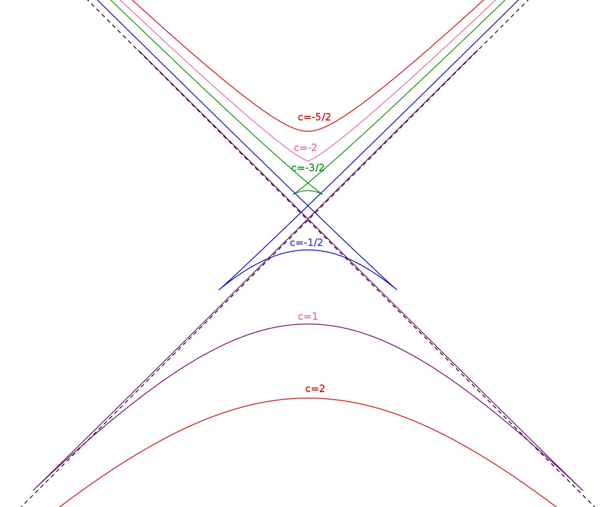
Figure 8: Plane $C^{2}$ hedgehogs with support function $h(t)=\cos(t)+c$ (curves are drawn thanks to (26)). If $c$ is sufficiently small or large, the hedgehog bounds an F-convex set or a P-convex set.

2.17 Elementary volume computations

For a space-like $C^{1}$ hypersurface $S$, we denote by $\mathrm{d}(S)$ the volume form of $S$ for the Riemannian metric induced on $S$ by the ambient Lorentzian metric.

Lemma 2.56.

Let $A$ be an open set of $\mathbb{R}^{d+1}$ and let $l:A\rightarrow\mathbb{R}$ be a $C^{1}$ function with non-vanishing gradient. Suppose that the level hypersurfaces $A_{t}:=l^{-1}(t)$ are space-like. Then

$$V(A)=\int\int_{A_{t}}\frac{1}{\|\operatorname{grad}_{x}l\|_{-}}\mathrm{d}(A_{t})(x)\mathrm{d}t.$$

The Lorentzian coarea formula formula above is certainly well-known in more general versions, nevertheless we provide a proof, just following the classical one, see e.g. [Sch93b]. The key elementary remarks are: 1) if we take $d$ space-like vectors with last coordinates equal to $0$ and a vertical vector, the computation of the volume of the resulting box is obviously the same for the Euclidean metric and for the Minkowski metric 2) linear Lorentzian isometries have determinant modulus equal to $1$ so they preserve the volume.

Proof.

The Lorentzian gradient of $l$ is a non-zero time-like vector. Without loss of generality we suppose that it is past directed. Moreover at a point $x_{0}\in A$ we have $\frac{\partial l}{\partial x_{d+1}}(x_{0})\not=0$. Up to a add a constant to $l$, let us suppose that $l(x_{0})=0$. By the implicit function theorem, locally there exists a $C^{1}$ map $g$ such that $x_{d+1}=g(x_{1},\ldots,x_{d},t)$ and

$$l(x_{1},\ldots,x_{d},g(x_{1},\ldots,x_{d},t))=t.$$

We define a $C^{1}$ diffeomorphism $\Phi$ from an open set $O\times(-\varepsilon,\varepsilon)$, $O\subset{\mathbb{R}}^{d}$, to $A$ by

$$(x_{1},\ldots,x_{d},t)\mapsto(x_{1},\ldots,x_{d},g(x_{1},\ldots,x_{d},t)).$$

(Up to decompose $A$ into suitable open sets, we suppose for simplicity that the image of $\Phi$ is the whole $A$.) Let us denote $X_{i}=\frac{\partial\Phi}{\partial x_{i}}$, $i=1,\ldots,d$ and $X_{d+1}=\frac{\partial\Phi}{\partial t}$. Then [Sch93b, 6.2.1]

$$V(A)=\int_{-\varepsilon}^{\varepsilon}\int_{O}|\operatorname{det}(X_{1},\ldots,X_{d+1})|\mbox{d}x_{1}\cdots\mbox{d}x_{d}\mbox{d}t.$$

The vectors $X_{1},\ldots,X_{d}$ belong to the space-like tangent space $L$ to $A_{t}$. Let $f_{1},\ldots,f_{d}$ be an orthonormal basis (for $\langle\cdot,\cdot\rangle_{-}$) of $L$, and $f_{d+1}$ be the unit past time-like vector orthogonal to $L$. We have

$$\operatorname{det}(X_{1},\ldots,X_{d+1})=\operatorname{det}\left(\langle X_{i},f_{j}\rangle_{-}\right)_{i,j=1,\ldots,d+1}$$

(this is easy to see using a Lorentz linear isometry sending $f_{1},\ldots,f_{d+1}$ to $e_{1},\ldots,e_{d},-e_{d+1}$ with $\{e_{i}\}$ the standard Euclidean basis —this isometry has determinant $1$). As $\langle X_{i},f_{d+1}\rangle_{-}=0$ for $i=1,\ldots,d$,

$$\operatorname{det}(X_{1},\ldots,X_{d+1})=\langle X_{d+1},f_{d+1}\rangle_{-}\operatorname{det}(\langle X_{i},f_{j}\rangle_{-})_{i,j=1,\ldots,d}.$$

On one hand,

$$\langle X_{d+1},f_{d+1}\rangle_{-}=\left\langle\frac{\partial\Phi}{\partial t},\frac{\mathrm{grad}l}{\|\mathrm{grad}l\|_{-}}\right\rangle_{-}=\frac{1}{\|\mathrm{grad}l\|_{-}}\left\langle\left(\begin{array}[]{c}0\\ \vdots\\ 0\\ \frac{\partial g}{\partial t}\end{array}\right),\mathrm{grad}h\right\rangle_{-}$$

$$=\frac{1}{\|\mathrm{grad}l\|_{-}}\frac{\partial g}{\partial t}\frac{\partial l}{\partial x_{d+1}}=\frac{1}{\|\mathrm{grad}l\|_{-}}.$$

On the other hand,

$$D:=\operatorname{det}(\langle X_{i},f_{j}\rangle_{-})_{i,j=1,\ldots,d}=-\operatorname{det}M$$

with

$$M={}^{t}\!(X_{1},\ldots,X_{d},f_{d+1})J(f_{1},\ldots,f_{d},f_{d+1}).$$

Note that $D=\operatorname{det}MJ$. So

$$-D^{2}=\operatorname{det}MJ\times{}^{t}M=\operatorname{det}{}^{t}\!(X_{1},\ldots,X_{d},f_{d+1})J(X_{1},\ldots,X_{d},f_{d+1})=\operatorname{det}(\langle X_{i},X_{j}\rangle_{-})_{i,j=1,\ldots,d},$$

finally $|D|=\sqrt{\left|\mathrm{det}\left(\langle\frac{\partial\Phi}{\partial x_{i}},\frac{\partial\Phi}{\partial x_{j}}\rangle_{-}\right)_{i,j=1,\ldots,d}\right|}$ and $|D|\mbox{d}x_{1}\cdots\mbox{d}x_{d}$ is the volume form on $A_{t}$ for the metric induced by the Lorentzian metric. ∎

3 Area measures

3.1 Definition of the area measures

3.1.1 Main statement

The notation is the one of Subsection 2.11. Let $\omega\subset{\mathbb{H}}^{d}$ be a Borel set. The normal field $N$ is continuous, and if we denote by $N_{\varepsilon}$ its restriction to $K_{(0,\varepsilon]}$, $K_{(0,\varepsilon]}(\omega)=N_{\varepsilon}^{-1}(\omega)$, so $K_{(0,\varepsilon]}(\omega)$ is measurable for the Lebesgue measure, and we denote by $V_{\varepsilon}(K,\omega)$ its volume. In other terms, $V_{\varepsilon}(K,\cdot)$ is the push forward of the restriction to $K_{(0,\varepsilon]}$ of the Lebesgue measure, which is a Radon measure, and as $N_{\varepsilon}$ is continuous, $V_{\varepsilon}(K,\cdot)$ is a Radon measure on ${\mathbb{H}}^{d}$. All results concerning measure theory in this section are elementary and can be found for example in [Tao10] or in the first pages of [Mat95]. Actually we mainly use these well known facts:

• Radon measures on ${\mathbb{H}}^{d}$ are the (unsigned) Borel measures which are finite on any compact,

• a Radon measure $\mu$ has the inner regularity property: for any Borel set $\omega$ of ${\mathbb{H}}^{d}$,

  $$\mu(\omega)=\operatorname{sup}\{\mu(K)|K\subset\omega,K\mbox{ compact }\},$$

• for any positive linear functional $I$ on the space of real continuous compactly supported functions on ${\mathbb{H}}^{d}$, there exists a unique Radon measure $\mu$ on ${\mathbb{H}}^{d}$ such that $I(f)=\int_{\mathbb{H}^{d}}f\operatorname{d}\mu$ (Riesz representation theorem).

The aim of this subsection is to prove the following result.

Theorem 3.1.

Let $K$ be an F-convex set in $\mathbb{R}^{d+1}$. There exist Radon measures $S_{0}(K,\cdot),\ldots,S_{d}(K,\cdot)$ on ${\mathbb{H}}^{d}$ such that, for any Borel set $\omega$ of ${\mathbb{H}}^{d}$ and any $\varepsilon>0$,

$$V_{\varepsilon}(K,\omega)=\frac{1}{d+1}\sum_{i=0}^{d}\varepsilon^{d+1-i}\binom{d+1}{i}S_{i}(K,\omega).$$ (28)

$S_{i}(K,\cdot)$ is called the area measure of order $i$ of $K$. We have that $S_{0}(K,\cdot)$ is given by the volume form of ${\mathbb{H}}^{d}$.

Two of those measures deserve special attention. $S_{d}(K,\cdot)$ may be called “the” area measure of $K$, for a reason which will be clear below. The problem of prescribing this measure is the Minkowski problem. In this paper we will focus on $S_{1}(K,\cdot)$.

Example 3.2.

For any $p\in{\mathbb{R}}^{d+1}$ let us consider $K={\mathcal{C}}(p)$. Actually $V_{\varepsilon}({\mathcal{C}}(p),\omega)$ is invariant under translations, so it suffices to compute it for $p=0$. From Lemma 2.56, using the cosmological time of the future cone (the Lorentzian distance to the origin), which has Lorentzian gradient equal to $1$,

$$V_{\varepsilon}({\mathcal{C}}(p),\omega)=\frac{\varepsilon^{d+1}}{d+1}S_{0}(K,\omega),$$ (29)

that expresses the fact that all space-like hyperplanes meet ${\mathcal{C}}(p)$ only at $p$, so the “curvatures” are supported only at a single point.

After some basics results on the $C^{1}$, $C^{2}_{+}$ and polyhedral cases, we will prove a statement close to Theorem 3.1 in the Fuchsian case. After that we will prove that, up to a translation, any compact part of the boundary of an F-convex set can be considered as a part of a Fuchsian convex set. The proof of Theorem 3.1 will follow from the following elementary remark.

Lemma 3.3.

The area measures defined in Theorem 3.1 are uniquely defined. They are even defined locally: if $K$ and $K^{\prime}$ are two F-convex sets such that the statement of Theorem 3.1 holds, and if $\omega$ is a Borel set of ${\mathbb{H}}^{d}$ with $K(\omega)=K^{\prime}(\omega)$, then $S_{i}(K,\omega)=S_{i}(K^{\prime},\omega)$.

Proof.

The uniqueness of the $S_{i}(K,\cdot)$ follows because (28) says that $V_{\varepsilon}(K,\omega)$ is a polynomial in $\varepsilon$. $K(\omega)=K^{\prime}(\omega)$ clearly implies $K_{(0,\varepsilon]}(\omega)=K^{\prime}_{(0,\varepsilon]}(\omega)$ hence $V_{\varepsilon}(K,\omega)=V_{\varepsilon}(K^{\prime},\omega)$, which are polynomials by Theorem 3.1, hence they have equal coefficients. ∎

Remark 3.4.

Due to their local nature, the area measures can be defined for more general convex sets than F-convex sets. What is needed is that the restriction of the normal map to level sets of the cosmological time is a proper map , see Subsection 2.11.

Remark 3.5.

From (28) we get a definition à la Minkowski for the area measure of an F-convex set:

$$\underset{\varepsilon\downarrow 0}{\mathrm{lim}}\frac{V_{\varepsilon}(K,\omega)-V_{0}(K,\omega)}{\varepsilon}=\underset{\varepsilon\downarrow 0}{\mathrm{lim}}\frac{V_{\varepsilon}(K,\omega)}{\varepsilon}=S_{d}(K,\omega).$$

Remark 3.6.

Let $K$ be a $C^{1}$ F-convex set and let $\mathrm{d}K$ be the volume form on $\partial_{s}K$ given by the Riemannian metric induced on $\partial_{s}K$ by the ambient Lorentzian metric. Let us denote by $\mbox{Area}(K,\omega)$ the measure (for $\mathrm{d}K$) of the set of points of $\partial_{s}K$ whose support vector belongs to $\omega$, i.e.  $\mbox{Area}(K,\omega)$ is the push-forward of $\mathrm{d}K$ on ${\mathbb{H}}^{d}$:

$$\mbox{Area}(K,\omega)=\mathrm{d}K(G_{K}^{-1}(\omega))=\mathrm{d}K(K(\omega))=(G_{K})_{*}\mathrm{d}K(\omega),$$

and $\mbox{Area}(K,\cdot)$ is a Borel measure because $G_{K}$ is continuous (Lemma 2.38). It is even a Radon measure as finite on any compact set, because if $\omega$ is compact then $K(\omega)$ is compact (see Section 2.11). Now, the cosmological time $T$ of any F-convex set $K$ is $C^{1}$, with Lorentzian gradient equal to $1$, so from Lemma 2.56:

$$V_{\varepsilon}(K,\omega)=\int_{0}^{\varepsilon}\mathrm{Area}(K_{t},\omega)\mbox{d}t.$$ (30)

Remark 3.7.

With the notation of Remark 2.42:

$$V_{\varepsilon}(K,\gamma_{0}\omega)=V_{\varepsilon}(K,\omega).$$ (31)

3.1.2 The $C^{2}_{+}$ case

Let $K$ be a $C^{2}_{+}$ F-convex set. We denote by $s_{i}$ the $i$th elementary symmetric function of the radii of curvature of $K$, i.e.

$$s_{i}=\binom{d}{i}^{-1}\sum_{1\leq j_{1}<\cdots<j_{i}\leq d}r_{j_{1}}\cdots r_{j_{i}}.$$

In particular $s_{0}=1$, $s_{1}=\frac{1}{d}(r_{1}+\cdots+r_{d})=\frac{1}{d}\mathrm{Trace}(S^{-1})$ and $s_{d}=r_{1}\cdots r_{d}=\mathrm{det}(S^{-1})$, where $S^{-1}$ is the reverse shape operator of $\partial K$.

Lemma 3.8.

Let $K$ be a $C^{2}_{+}$ F-convex set. Then the statement of Theorem 3.1 holds. Moreover

$$S_{i}(K,\cdot)=s_{i}\mathrm{d}\mathbb{H}^{d}(\cdot).$$

Proof.

$K_{t}$ is the boundary of $K+tK({\mathbb{H}})$, which is $C^{2}_{+}$ by (2) of Corollary 2.48. The Gauss map is a $C^{1}$ diffeomorphism hence

$$\int_{K_{t}(\omega)}\mbox{d}K_{t}=\int_{\omega}\mathrm{det}(S^{-1}_{t})\mbox{d}\mathbb{H}^{d}$$ (32)

where $S^{-1}_{t}$ is the reverse shape operator of the boundary of $K+tK({\mathbb{H}})$. Moreover from (21) $S^{-1}_{t}=S^{-1}+t\mathrm{Id}$. The result follows using (30) and

$$\mathrm{det}(S^{-1}+t\mathrm{Id})=\sum_{k=0}^{d}t^{k}\binom{d}{k}s_{d-k}.$$

∎

Remark 3.9.

(32) can be written $\mbox{Area}(K,\omega)=S_{d}(K,\omega)$, that explains the terminology for “the” area measure $S_{d}$.

3.1.3 The polyhedral case

The following characterization of the area measures for the compact case seemlingly appeared in [Zel70], see also [Fir70]. Let $P$ be a polyhedral F-convex set. For a $i$-face $e_{i}$, we denote by $\lambda_{i}(e_{i})$ the $i$-dimensional volume of $e_{i}$ in the Euclidean space isometric to the support plane containing $e_{i}$. We also denote by $\nu_{n}$ the $n$-dimensional Hausdorff measure of ${\mathbb{H}}^{d}$.

Lemma 3.10.

Let $P$ be a polyhedral F-convex set. Then the statement of Theorem 3.1 holds. Moreover, for any Borel set $\omega\subset{\mathbb{H}}^{d}$,

$$S_{i}(P,\omega)=\binom{d}{i}^{-1}\sum_{e_{i}}\lambda_{i}(e_{i})\nu_{d-i}(\omega\cap G_{P}(e_{i})).$$ (33)

where the sum is on all the open $i$-faces $e_{i}$ of $P$ and $G_{P}$ is the Gauss map of $P$.

Proof.

Let $e_{i}$ be an open $i$-face of $P$ and let $\omega$ be a Borel subset in the relative interior of $G_{P}(e_{i})$. We have

$$V_{\varepsilon}(P,\omega)=\lambda_{i}(e_{i})\frac{\nu_{d-i}(\omega)\varepsilon^{d+1-i}}{d+1-i}.$$

Indeed, up to a volume preserving Lorentzian isometry, we can suppose that the hyperplane containing $e_{i}$ is an horizontal hyperplane, for which the induced metric for the Euclidean or the Lorentzian structure of ${\mathbb{R}}^{d+1}$ are the same. By Fubini Theorem,

$$V_{\varepsilon}(P,\omega)=V((e_{i})_{(0,\varepsilon]},\omega)=\int_{e_{i}}V_{d+1-i}({\mathcal{C}}(x)_{(0,\varepsilon)}(\omega)))\mathrm{d}V_{i}(x)$$

where $V_{k}$ is the volume in ${\mathbb{R}}^{k}$. The relation (29) gives that $V_{d+1-i}({\mathcal{C}}(x)_{(0,\varepsilon)}(\omega)))=\frac{\varepsilon^{d+1-i}}{d+1-i}\nu_{d-i}(\omega)$, which is independent of $x$.

Now, if $e_{i}$ and $e_{j}$ are distinct open faces of $P$, then for any $\omega_{i}\subset G_{P}(e_{i})$ and $\omega_{j}\subset G_{P}(e_{j})$, for any positive $\varepsilon$, the interiors of $P_{(0,\varepsilon]}(\omega_{i})$ and $P_{(0,\varepsilon]}(\omega_{j})$ are disjoint. On one hand, $V_{\varepsilon}(P,\cdot)$ and $\nu_{d-i}$ are measures on ${\mathbb{H}}^{d}$. On the other hand, the cell decomposition of ${\mathbb{H}}^{d}$ given by $P$ has a countable number of cells, and each face is defined as the intersection of a finite number of cells, hence the decomposition has a countable number of faces. By the property of countable additivity of measures, we get, for any Borel set $\omega\subset{\mathbb{H}}^{d}$:

$$V_{\varepsilon}(P,\omega)=\sum_{i=0}^{d}\frac{1}{d+1-i}\sum_{e_{i}}\lambda_{i}(e_{i})\nu_{d-i}(\omega\cap G_{P}(e_{i}))\varepsilon^{d+1-i}.$$

The lemma follows by comparing the coefficients with (28). ∎

3.2 The Fuchsian case

We prove a “quotiented” version of Theorem 3.1. By the strong analogy between Fuchsian convex sets and convex bodies, the argument is a straightforward adaptation of Chapter 4 of [Sch93a].

Let $\Gamma$ be a group of hyperbolic isometries, such that ${\mathbb{H}}^{d}/\Gamma$ is a compact hyperbolic manifold. Let $K$ be a Fuchsian convex set (for the group $\Gamma$). Recall that $V_{\varepsilon}(K,\cdot)$ is then $\Gamma$ invariant. This permits to introduce a canonical projected Radon measure $V_{\varepsilon}^{\Gamma}(K,\cdot)$ on the Borel sets of ${\mathbb{H}}^{d}/\Gamma$. Namely, it is the only measure on ${\mathbb{H}}^{d}/\Gamma$ such that if $\omega\subset{\mathbb{H}}/\Gamma$ is a Borel set and $\psi:\omega\to{\mathbb{H}}^{d}$ is a measurable section of the covering projection $\pi:{\mathbb{H}}^{d}\to{\mathbb{H}}^{d}/\Gamma$, then $\psi_{\ast}(V_{\varepsilon}^{\Gamma}(K,\cdot))=V_{\varepsilon}(K,\cdot)$, [BF14, Section 3.4]. In particular it satisfies

$$V_{\varepsilon}^{\Gamma}(K,\pi(\omega))=V_{\varepsilon}(K,\omega)$$

each time $\omega$ meets at most once each orbit of $\Gamma$.

Let us denote by $\mathcal{K}(\Gamma)$ the set of $\Gamma$-F-convex sets. Recall that for $K,K^{\prime}\in\mathcal{K}(\Gamma)$, the Hausdorff distance between them is [Fil13]

$$d_{H}(K,K^{\prime})=\min\{\lambda\geq 0|K^{\prime}+\lambda K({\mathbb{H}})\subset K,K+\lambda K({\mathbb{H}})\subset K^{\prime}\}.$$

If $K\in\mathcal{K}(\Gamma)$, the covolume of $K$, $\mathrm{covol}_{\Gamma}(K)$, is the volume of $({\mathcal{F}}\setminus K)/\Gamma$. Note that

$$V_{\varepsilon}^{\Gamma}(K,{\mathbb{H}}^{d}/\Gamma)=\mathrm{covol}_{\Gamma}(K_{\varepsilon})-\mathrm{covol}_{\Gamma}(K).$$ (34)

Lemma 3.11.

Let $(K(n))_{n}$ be a sequence of $\Gamma$-convex sets converging (for $d_{H}$) to a $\Gamma$-convex set $K$. Then $V_{\varepsilon}^{\Gamma}(K(n),\cdot)$ weakly converges to $V_{\varepsilon}^{\Gamma}(K,\cdot)$.

Proof.

We have to prove that

1. $V_{\varepsilon}^{\Gamma}(K(n),{\mathbb{H}}^{d}/\Gamma)$ converges to $V_{\varepsilon}^{\Gamma}(K,{\mathbb{H}}^{d}/\Gamma)$,

2. for any open set $\omega$ of ${\mathbb{H}}^{d}/\Gamma$ then $\operatorname{Liminf}_{n\rightarrow+\infty}V_{\varepsilon}^{\Gamma}(K(n),\omega)\geq V_{\varepsilon}^{\Gamma}(K,\omega)$.

Note that $K_{\varepsilon}(n)=K(n)+\varepsilon K({\mathbb{H}})$ so by continuity of the Minkowski addition, $K_{\varepsilon}(n)$ converges to $K_{\varepsilon}$. By continuity of the covolume [Fil13], the first point follows from (34). Let us prove the second point. Let $\omega$ be an open set of ${\mathbb{H}}^{d}/\Gamma$, $\tilde{\omega}$ be any of its lift and let $x\in K_{(0,\varepsilon)}(\tilde{\omega})$.

Fact: for $n$ sufficiently large, $x\in K(n)_{(0,\varepsilon]}(\tilde{\omega})$.

Let us suppose that the Hausdorff distance between $K$ and $K(n)$ is $\delta$, the orthogonal projection of $x$ onto $\partial K$ is $p$ and $d_{L}(x,p)=t<\varepsilon$. Let us denote by $\eta\in\tilde{\omega}$ the vector $(x-p)/t$. As $K+\delta K({\mathbb{H}})\subset K(n)$, the point $q=p+\delta\eta$ belongs to $K(n)$. We can suppose that $\delta$ is small enough so that $\delta<t$ and then $x=p+t\eta$ belongs to $K(n)$. We denote by $p_{n}$ the orthogonal projection of $x$ onto $\partial K(n)$. By maximization property, $d_{L}(p_{n},x)\geq d_{L}(x,q)=t-\delta$. Note that $p$ and $p_{n}$ are both in the past cone of $x$. Up to a translation we can suppose that $x=0$. The last equation writes $\|p_{n}\|_{-}\geq t-\delta$. The property $K(n)+\delta K({\mathbb{H}})\subset K$ implies $\langle p_{n},\eta\rangle_{-}\leq H_{K}(\eta)+\delta$ with $H_{K}$ the extended support function of $K$, that can be written $\langle p_{n},\eta\rangle_{-}\leq t+\delta$.

We want to show that $-p_{n}/\|p_{n}\|_{-}$ is arbitrary close to $\eta$ if $n$ is sufficiently large (recall that $p_{n}$ is a past vector), i.e. that $\cosh d_{{\mathbb{H}}^{d}}(-p_{n}/\|p_{n}\|_{-},\eta)$ is close to $1$, i.e. that $\langle p_{n}/\|p_{n}\|_{-},\eta\rangle_{-}$ is close to $1$. But

$$\frac{\langle p_{n},\eta\rangle_{-}}{\|p_{n}\|}\leq\frac{t+\delta}{t-\delta}$$

that goes to $1$ when $\delta$ goes to $0$. On the other hand, $\|p_{n}\|_{-}\leq\langle p_{n},\eta\rangle_{-}$ as it can be easily checked. As $\tilde{\omega}$ is open, for $n$ sufficiently large $-p_{n}/\|p_{n}\|_{-}\in\tilde{\omega}$. Moreover

$$\|p_{n}\|_{-}\leq\langle p_{n},\eta\rangle_{-}\leq t+\delta$$

that is less than $\varepsilon$ if $\delta$ is sufficiently small because $t<\varepsilon$, so $d_{L}(p_{n},x)=\|p_{n}\|_{-}<\varepsilon$. The fact is proved.

The fact says that $K_{(0,\varepsilon)}(\tilde{\omega})\subset\operatorname{Liminf}_{n}K(n)_{(0,\varepsilon)}(\tilde{\omega})$, hence

$$V(K_{(0,\varepsilon)}(\tilde{\omega}))\leq V(\operatorname{Liminf}_{n}K(n)_{(0,\varepsilon)}(\tilde{\omega}))\leq\operatorname{Liminf}_{n}V(K(n)_{(0,\varepsilon)}(\tilde{\omega}))$$

that implies point 2 because the boundary of a convex set has zero Lebesgue measure. ∎

Lemma 3.12.

Let $K$ be a $\Gamma$ convex set. Then there exists a sequence of $\Gamma$-convex polyhedra converging to $K$.

Proof.

Let $\varepsilon>0$, $h$ be the support function of $K$ and $k_{i}\in\partial_{s}K$. There exists $\eta\in{\mathbb{H}}^{d}$ such that $\langle k_{i},\eta\rangle_{-}=h(\eta)$. By continuity there exists an open neighborhood $V_{i}$ of $\eta$ in ${\mathbb{H}}^{d}$ such that $|\langle k_{i},\eta^{\prime}\rangle_{-}-h(\eta^{\prime})|<\varepsilon,\,\forall\eta^{\prime}\in V_{i}$. By cocompactness of $\Gamma$, there exists a finite number of neighborhood $V_{i}$ as above such that $\{\Gamma V_{i}\}$ covers ${\mathbb{H}}^{d}$. The associated set of points $\{\Gamma k_{i}\}$ is discrete as discrete orbits of a finite number of points.

Let us introduce $h_{\varepsilon}(\eta)=\operatorname{max}_{i}\langle k_{i},\eta\rangle_{-}$. It is easy to see that if $\eta\in V_{i}$ and $\eta\notin V_{j}$, then $\langle\eta,k_{j}\rangle_{-}<\langle\eta,k_{i}\rangle_{-}$. Moreover each $\eta$ belongs to a finite number of $V_{i}$ (the tessellation of ${\mathbb{H}}^{d}$ by fundamental domains for $\Gamma$ is locally finite), hence $h_{\varepsilon}$ is well defined. It is also clearly $\Gamma$ invariant, hence it is the support function of a $\Gamma$ convex polyhedron and by construction, on ${\mathbb{H}}^{d}$, $|h_{\varepsilon}(\eta)-h(\eta)|<\varepsilon$. ∎

Proposition 3.13.

Let $K$ be a $\Gamma$ convex set. There exists finite Radon measures $S^{\Gamma}_{0}(K,\cdot),\ldots,S^{\Gamma}_{d}(K,\cdot)$ on ${\mathbb{H}}^{d}/\Gamma$ such that, for any Borel set $\omega$ of ${\mathbb{H}}^{d}/\Gamma$ and any $\varepsilon>0$,

$$V_{\varepsilon}^{\Gamma}(K,\omega)=\frac{1}{d+1}\sum_{i=0}^{d}\varepsilon^{d+1-i}\binom{d+1}{i}S_{i}^{\Gamma}(K,\omega),$$ (35)

and $S_{0}^{\Gamma}(K,\cdot)$ is given by the volume form on ${\mathbb{H}}^{d}/\Gamma$.

Moreover, if $K(n)$ converges to $K$, then $S_{i}^{\Gamma}(K(n),\cdot)$ weakly converges to $S_{i}^{\Gamma}(K,\cdot)$.

Proof.

If $P$ is a $\Gamma$ Fuchsian polyhedron, then (35) is a consequence of (33), applied to any lifting of $\omega$. By polynomial interpolation, for $d+1$ distinct reals numbers $n_{0},\ldots,n_{d}$, (35) applied with $\varepsilon=n_{i}$ can be considered as a solvable system of $d+1$ linear equations with unknowns $S_{0}^{\Gamma}(P,\omega),\ldots,S_{d}^{\Gamma}(P,\omega)$. So there exists real numbers $a_{im}$ with

$$S_{i}^{\Gamma}(P,\omega)=\sum_{m=0}^{d}a_{im}V_{n_{m}}^{\Gamma}(P,\omega).$$

Now let $K$ be any $\Gamma$-convex set. We define

$$S_{i}^{\Gamma}(K,\cdot):=\sum_{m=0}^{d}a_{im}V_{n_{m}}^{\Gamma}(K,\cdot).$$

Clearly $S_{i}^{\Gamma}(K,\cdot)$ is a finite signed Radon measure on ${\mathbb{H}}^{d}/\Gamma$. From Lemma 3.12 we can consider a sequence $P(n)$ of $\Gamma$-convex polyhedra converging to $K$, and from Lemma 3.11, for any continuous function $f$ on ${\mathbb{H}}^{d}/\Gamma$,

$$\int_{{\mathbb{H}}^{d}/\Gamma}f\operatorname{d}S_{i}^{\Gamma}(P(n),\cdot)\rightarrow\int_{{\mathbb{H}}^{d}/\Gamma}f\operatorname{d}S_{i}^{\Gamma}(K,\cdot).$$

It follows that $f\mapsto\int_{{\mathbb{H}}^{d}/\Gamma}f\operatorname{d}S_{i}^{\Gamma}(K,\cdot)$ is a positive linear functional, hence $S_{i}^{\Gamma}(K,\cdot)$ is a Radon measure.

The statement about weak convergence is clear. Using again polyhedral approximation and the fact that (35) is true in the polyhedral case, we see that the functionals on the continuous functions of ${\mathbb{H}}^{d}/\Gamma$ given by integrating with respect to each side of (35) are equal, hence the measures are equal by the uniqueness part of the Riesz representation theorem. We also get the remark on $S_{0}^{\Gamma}$ from Lemma 3.10. ∎

Remark 3.14 (A Steiner formula).

Let us introduce

$$W_{i}^{\Gamma}(K)=\frac{1}{d+1}S_{d+1-i}^{\Gamma}(K,{\mathbb{H}^{d}/\Gamma})$$

and $W_{0}^{\Gamma}(K):=\operatorname{covol}_{\Gamma}(K)$. They are the $\Gamma$-quermass integrals of $K$. Then (35) gives the following Steiner formula for $\Gamma$ convex sets:

$$V_{\varepsilon}(K)=\sum_{i=1}^{d+1}\varepsilon^{i}\binom{d+1}{i}W_{i}(K).$$

Note that $S_{0}^{\Gamma}(K,{\mathbb{H}}^{d}/\Gamma)=(d+1)W_{d+1}^{\Gamma}(K)$ is nothing but the volume of ${\mathbb{H}}^{d}/\Gamma$, which is itself related to the Euler characteristic of ${\mathbb{H}}^{d}/\Gamma$ if $d$ is even by the Gauss–Bonnet formula [Rat06]. In the compact Euclidean case, up to a dimensional constant the quermass integrals are the intrinsic volumes, and their sum has an integral representation known as Wills functional, see e.g. [Kam09].

Remark 3.15 (Mixed-area).

Recall that $\mathcal{K}(\Gamma)$ is the set of $\Gamma$-convex sets. The mixed-covolume $\mathrm{covol}(\cdot,\ldots,\cdot)$ is the unique symmetric $(d+1)$-linear form on $\mathcal{K}(\Gamma)$, continuous on each variable, such that [Fil13]

$$\mathrm{covol}(K,\ldots,K)=\mathrm{covol}(K).$$

For given $K_{1},\ldots,K_{d}\in\mathcal{K}(\Gamma)$, we get an additive functional

$$\mathrm{covol}(\cdot,K_{1},\ldots,K_{d}):\mathcal{K}(\Gamma)\rightarrow{\mathbb{R}},K\mapsto\mathrm{covol}(K,K_{1},\ldots,K_{d}).$$

If we identify the $\Gamma$-convex sets with their support functions, we can consider $\mathcal{K}(\Gamma)$ as a subset of $C^{0}({\mathbb{H}}^{d}/\Gamma)$, the set of continuous functions on ${\mathbb{H}}^{d}/\Gamma$. Following the classical arguments of the compact case [Ale37], one can show that $\mathrm{covol}(\cdot,K_{1},\ldots,K_{d})$ can be extended to a positive linear functional on $C^{0}({\mathbb{H}}^{d}/\Gamma)$. The first step is to extend $\mathrm{covol}(\cdot,K_{1},\ldots,K_{d})$ to the subset of $C^{0}({\mathbb{H}}^{d}/\Gamma)$ of functions which are difference of support functions: if $Z=h_{1}-h_{2}$ where $h_{1}$ and $h_{2}$ are support functions of $\Gamma$ convex sets, then we define

$$\mathrm{covol}(Z,K_{1},\ldots,K_{d})=\mathrm{covol}(h_{1},K_{1},\ldots,K_{d})-\mathrm{covol}(h_{2},K_{1},\ldots,K_{d}).$$

By the Stone–Weierstrass theorem, any continuous function on ${\mathbb{H}}^{d}/\Gamma$ can be uniformly approximated by a $C^{2}$ function. Moreover any $C^{2}$ function $Z$ on ${\mathbb{H}}^{d}/\Gamma$ is the difference of two support functions: for $t$ sufficiently large, $Z+t$ satisfies (22). Hence any continuous function on ${\mathbb{H}}^{d}/\Gamma$ can be uniformly approximated by the difference of two support functions. From this it can be checked that $\mathrm{covol}(\cdot,K_{1},\ldots,K_{d})$ can be extended to $C^{0}({\mathbb{H}}^{d}/\Gamma)$ with the required properties.

By the Riesz representation theorem there exists a unique Radon measure on ${\mathbb{H}}^{d}/\Gamma$, the mixed-area measure, denoted by $S(K_{1},\ldots,K_{d};\cdot)$, such that, for any $f\in C^{0}({\mathbb{H}}^{d}/\Gamma)$,

$$\mathrm{covol}(f,K_{1},\ldots,K_{d})=-\frac{1}{d+1}\int_{\mathbb{H}^{d}/\Gamma}f(u)\mathrm{d}S(K_{1},\ldots,K_{d};u).$$

The mixed-area measures are generalization of the area measures in the Fuchsian case. Let us sketch the proof of this fact. Following [FJ38], p. 29, one can prove that

$$S(K,\cdots,K;\omega)=\underset{\varepsilon\downarrow 0}{\mathrm{lim}}\frac{V_{\varepsilon}(K,\omega)}{\varepsilon}$$

It is clear that $K_{(0,\varepsilon+t]}(\omega)$ is the disjoint union of $K_{(0,\varepsilon]}(\omega)$ and of $(K_{\varepsilon})_{(0,t]}(\omega)$, in particular

$$V_{\varepsilon+t}(K,\omega)=V_{t}(K,\omega)+V_{\varepsilon}(K_{t},\omega)$$

hence the equation above can be written

$$\underset{\varepsilon\downarrow 0}{\mathrm{lim}}\frac{V_{\varepsilon+t}(K,\omega)-V_{t}(K,\omega)}{\varepsilon}=S(K+tK({\mathbb{H}}),\cdots,K+tK({\mathbb{H}}),\omega),$$

with $K({\mathbb{H}})$ the $\Gamma$-convex set bounded by ${\mathbb{H}}^{d}$, in other terms

$$S(K+tK({\mathbb{H}}),\cdots,K+tK({\mathbb{H}}),\omega)=\frac{d}{d\varepsilon}\left(V_{\varepsilon}(K,\omega)\right)(t).$$

On the other hand, by properties of the mixed-covolume, $S(K_{1},\ldots,K_{d};\cdot)$ is linear in each variable, in particular,

$$S(K+tK({\mathbb{H}}),\ldots,K+tK({\mathbb{H}});\cdot)=\sum_{i=0}^{d}t^{d-i}\binom{d}{i}S(\underbrace{K,\ldots,K}_{i},K({\mathbb{H}}),\ldots,K({\mathbb{H}});\cdot),$$

Integrating the two equations above between $0$ and $\varepsilon$ with respect to $t$ leads to

$$V_{\varepsilon}(K,\omega)=\frac{1}{d+1}\sum_{i=0}^{d}\varepsilon^{d+1-i}\binom{d+1}{i}S(\underbrace{K,\ldots,K}_{i},K({\mathbb{H}}),\ldots,K({\mathbb{H}});\omega),$$

Comparing the coefficients with (35) leads to

$$S(\underbrace{K,\ldots,K}_{i},K({\mathbb{H}}),\ldots,K({\mathbb{H}});\cdot)=S_{i}^{\Gamma}(K,\cdot).$$

Remark 3.16.

With the notations of Remark 3.14

$$W_{d}(K)=\frac{1}{d+1}S_{1}^{\Gamma}(K,{\mathbb{H}^{d}/\Gamma})=\int_{{\mathbb{H}^{d}/\Gamma}}\mathrm{d}S(K,K({\mathbb{H}}),\ldots,K({\mathbb{H}}))=\operatorname{covol}(K({\mathbb{H}}),K,K({\mathbb{H}}),\ldots,K({\mathbb{H}}))=$$

$$=\operatorname{covol}(K,K({\mathbb{H}}),\ldots,K({\mathbb{H}}))=-\int_{{\mathbb{H}^{d}/\Gamma}}h\mathrm{d}S(K({\mathbb{H}}),\ldots,K({\mathbb{H}}))=-\int_{{\mathbb{H}^{d}/\Gamma}}h\mathrm{d}{\mathbb{H}}^{d}/\Gamma$$

(in the $C^{2}_{+}$ case, writing the first area measure with the help of the Laplacian — see (1) —, it appears that the formula above is nothing but the Green Formula $\int_{{\mathbb{H}^{d}/\Gamma}}h\Delta f=\int_{{\mathbb{H}^{d}/\Gamma}}f\Delta h$ applied to $f=-1$). See also Subsection 5.3.

Remark 3.17 (Mean radius of curvature and Hessian of the covolume).

As in the compact Euclidean case, the Hessian of the covolume of $C^{\infty}_{+}$ Fuchsian convex sets, at the point $K({\mathbb{H}})$, is $(S_{1}(\cdot),\cdot)$, where $(\cdot,\cdot)$ is the $L^{2}$ scalar product on ${\mathbb{H}}^{d}/\Gamma$, see [Fil13] — it acts on the space of $C^{\infty}$ functions on ${\mathbb{H}}^{d}/\Gamma$, i.e. on the space of $C^{\infty}$ $\Gamma$-hedgehogs.

3.3 Fuchsian extension

Lemma 3.18.

Let $K$ be an F-convex set and $\omega\subset{\mathbb{H}}^{d}$ be a bounded Borel set. Up to a translation, there exists a Fuchsian convex set $\tilde{K}_{\omega}$ such that, for any subset $\omega^{\prime}$ of $\omega$,

$$K(\omega^{\prime})=\tilde{K}_{\omega}(\omega^{\prime}).$$

$\tilde{K}_{\omega}$ is a $\omega$-Fuchsian extension of $K$.

Proof.

Let $\boldsymbol{\omega}$ be a compact set of ${\mathbb{H}}^{d}$ containing $\omega$ in its interior. As $K(\boldsymbol{\omega})$ is compact (see Subsection 2.11), up to a translation, we suppose $K(\boldsymbol{\omega})\subset{\mathcal{F}}$. This implies that the support function $h_{K}$ of $K$ is negative on $\boldsymbol{\omega}$ (for $x\in K(\boldsymbol{\omega})$ with support vector $\eta\in\boldsymbol{\omega}$ we have $h_{K}(\eta)=\langle\eta,x\rangle_{-}<0)$. Let $h_{0}$ be the infimum of $h_{K}$ on $\boldsymbol{\omega}$. Let $B_{\rho}$ be the closed ball of ${\mathbb{H}}^{d}$ of radius $\rho$ centered at $e_{d+1}$.

Fact: $\exists\rho>0,\forall x\in K(\boldsymbol{\omega}),\forall\eta\in{\mathbb{H}}^{d}\setminus B_{\rho},\langle x,\eta\rangle_{-}\leq h_{0}$.

The condition $\langle x,\eta\rangle_{-}\leq h_{0}$ can be written

$$\cosh d_{{\mathbb{H}}^{d}}\left(\frac{x}{\|x\|_{-}},\eta\right)\geq\frac{|h_{0}|}{\|x\|_{-}}.$$

As $K(\boldsymbol{\omega})$ is compact and contained in ${\mathcal{F}}$, $\{x/\|x\|_{-}|x\in K(\boldsymbol{\omega})\}$ is a compact set of ${\mathbb{H}}^{d}$, say contained in $B_{r}$. Any $\rho$ larger than $\displaystyle r+\frac{|h_{0}|}{\underset{x\in K(\boldsymbol{\omega})}{\mathrm{inf}}(\|x\|_{-})}$ satisfies the wanted condition. The fact is proved.

Let $\Gamma$ be a group of isometries such that ${\mathbb{H}}^{d}$ is compact and containing $B_{\rho}$ in a fundamental domain (this is always possible, see page 74 of [Far96]). We define

$$\tilde{K}_{\omega}:=\{x\in{\mathbb{R}}^{d+1}|\langle x,\eta\rangle_{-}\leq h_{K}(\gamma_{0}^{-1}\eta),\forall\eta=\gamma_{0}\eta_{0},\gamma_{0}\in\Gamma,\eta_{0}\in\boldsymbol{\omega}\},$$ (36)

i.e. $\tilde{K}_{\omega}$ is the intersection of the future side of the support planes of $K(\omega)$ and of their orbits for the action of $\Gamma$. Because of the choice of $\Gamma$, $K(\boldsymbol{\omega})\subset\tilde{K}_{\omega}$. Moreover it is clear that the support planes of $K(\boldsymbol{\omega})$ are support planes of $\tilde{K}_{\omega}$, hence $K(\boldsymbol{\omega})\subset\tilde{K}_{\omega}(\boldsymbol{\omega})$ (note that the inclusion may be strict). Finally $\tilde{K}_{\omega}$ is different from $\overline{{\mathcal{F}}}$, it is $\Gamma$-invariant and it is an F-convex set (Lemma 2.6) hence it is a $\Gamma$-F-convex set.

Finally, we prove below that $K(\stackrel{{\scriptstyle\circ}}{{\boldsymbol{\omega}}})=\tilde{K}_{\omega}(\stackrel{{\scriptstyle\circ}}{{\boldsymbol{\omega}}})$. Obviously this implies that for any subset $\omega^{\prime}$ of $\stackrel{{\scriptstyle\circ}}{{\boldsymbol{\omega}}}$, we have $K(\omega^{\prime})=\tilde{K}_{\omega}(\omega^{\prime})$.

Suppose that $K(\stackrel{{\scriptstyle\circ}}{{\boldsymbol{\omega}}})\not=\tilde{K}_{\omega}(\stackrel{{\scriptstyle\circ}}{{\boldsymbol{\omega}}})$. As $K(\stackrel{{\scriptstyle\circ}}{{\boldsymbol{\omega}}})\subset\tilde{K}_{\omega}(\stackrel{{\scriptstyle\circ}}{{\boldsymbol{\omega}}})$, this means that there exists $y\in\partial\tilde{K}_{\omega}$, $y\notin K(\stackrel{{\scriptstyle\circ}}{{\boldsymbol{\omega}}})$ and $\eta\in G_{\tilde{K}_{\omega}}(y)\cap\stackrel{{\scriptstyle\circ}}{{\boldsymbol{\omega}}}$. Let $\mathcal{H}$ be the support hyperplane of $K$ orthogonal to $\eta$. $\mathcal{H}\cap K=K(\{\eta\})$ is a convex compact set (see Lemma 2.8). Let $x$ be the orthogonal projection (in $\mathcal{H}$) of $y$ onto $\mathcal{H}\cap K$. Let us denote by $v$ the normalization of the space-like vector $y-x$ and by $H$ the extended support function of $K$ (which is equal to the extended support function of $\tilde{K}_{\omega}$ on $\boldsymbol{\omega}$). We also denote by $H^{\prime}(\eta;v)$ the one-sided directional derivative of $H$ at $\eta$ in the direction $v$. By [Sch93a, 1.7.2] (see the proof of [Fil13, 3.1] for the Lorentzian version) it is equal to the total support function of $\mathcal{H}\cap K$ evaluated at $v$, hence it is equal to $\langle x,v\rangle_{-}$.

As $\eta$ is in the interior of $\boldsymbol{\omega}$, for small positive $\varepsilon$, the projection of $\eta+\varepsilon v$ onto ${\mathbb{H}}^{d}$ is in $\boldsymbol{\omega}$. We want to find the non-negative $\lambda(\varepsilon)$, depending on $\varepsilon$, such that

$$\langle x+\lambda(\varepsilon)v,\eta+\varepsilon v\rangle_{-}=H(\eta+\varepsilon v).$$ (37)

We get (recall that $\langle v,\eta\rangle_{-}=0$)

$$\lambda(\varepsilon)=\frac{H(\eta+\varepsilon v)-\langle x,\eta\rangle_{-}}{\varepsilon}-\langle x,v\rangle_{-}.$$

which is non-negative because

$$\langle x,\eta+\varepsilon v\rangle_{-}\leq H(\eta+\varepsilon v),$$

(that only means that $x$ belongs to $K$) and clearly continuous on positive $\varepsilon$.

Moreover

$$\lambda(\varepsilon)=\frac{H(\eta+\varepsilon v)-H(\eta)}{\varepsilon}-\langle x,v\rangle_{-}$$

and $\underset{\varepsilon\downarrow 0}{\mathrm{lim}}\lambda(\varepsilon)=H^{\prime}(\eta;v)-\langle x,v\rangle_{-}=0$.

Hence one can find $\varepsilon$ such that $x+\lambda(\varepsilon)v$ is between $x$ and $y$ and different from $y$. But (37) says that $x+\lambda(\varepsilon)v$ is the intersection between the support hyperplane of $K(\boldsymbol{\omega})$ orthogonal to $\eta+\varepsilon v$ and the line between $x$ and $y$: $y$ is not on the same side of a support plane of $K(\boldsymbol{\omega})$ (and hence of $\tilde{K}_{\omega}$) than $x$, that is impossible. ∎

Lemma 3.19.

Let $K_{1},K_{2}$ be two F-convex sets with extended support functions $H_{1},H_{2}$ and $\boldsymbol{\omega}$ a compact set of ${\mathbb{H}}^{d}$ and $\varepsilon>0$ with $\mathrm{sup}_{\eta\in\boldsymbol{\omega}}|H_{1}(\eta)-H_{2}(\eta)|<\varepsilon$.

Then for any compact set $\omega$ in the interior of $\boldsymbol{\omega}$ there exists an isometry group $\Gamma$ acting cocompactly on ${\mathbb{H}}^{d}$ and $\omega$-$\Gamma$ extensions $\tilde{K_{1}}$ and $\tilde{K_{2}}$ of respectively $K_{1}$ and $K_{2}$ such that $d_{H}(\tilde{K_{1}},\tilde{K_{2}})<\varepsilon$.

Proof.

Using the same notations as in the proof of Lemma 3.18, we take as $\Gamma$ a group containing $B_{\mathrm{max}(\rho_{K_{1}},\rho_{K_{2}})}$ in a fundamental domain. Let $y\in\tilde{K_{1}}+\varepsilon K({\mathbb{H}})$: $y=x+\varepsilon b$ with $x\in\tilde{K_{1}}$ and $b\in K({\mathbb{H}})$. Let $\eta\in{\mathbb{H}}^{d}$ such that $\eta=\gamma_{0}\eta_{0}$ with $\gamma_{0}\in\Gamma$ and $\eta_{0}\in\boldsymbol{\omega}$. We have

$$\langle y,\eta\rangle_{-}=\langle x,\eta\rangle_{-}+\varepsilon\langle b,\eta\rangle_{-}\leq H_{1}(\eta_{0})-\varepsilon\leq H_{2}(\eta_{0})=H_{2}(\gamma_{0}^{-1}\eta),$$

because $\langle b,\eta\rangle_{-}\leq-1$, hence $y\in\tilde{K_{2}}$ by definition (36), and $\tilde{K_{1}}+\varepsilon K({\mathbb{H}})\subset\tilde{K_{2}}$. In the same way $\tilde{K_{2}}+\varepsilon K({\mathbb{H}})\subset\tilde{K_{1}}$, so by definition $d_{H}(\tilde{K_{1}},\tilde{K_{2}})<\varepsilon$. ∎

3.4 Proof of Theorem 3.1

Let $\omega\subset{\mathbb{H}}^{d}$ be compact, and consider $\tilde{K}_{\omega}$ as in Lemma 3.18 (clearly, $V_{\varepsilon}(K,\omega)$ is invariant under translation). Let us define the following Radon measures on $\omega$: for any Borel set $b$ contained in $\omega$ and $i\in\{1,\ldots,d\}$

$$S_{i}^{\omega}(K,b):=S^{\Gamma}_{i}(\tilde{K}_{\omega},\overline{b}),$$ (38)

with $\overline{b}$ the image of $b$ for the projection ${\mathbb{H}}^{d}\rightarrow{\mathbb{H}}^{d}/\Gamma$ and $S^{\Gamma}_{i}(\tilde{K}_{\omega},\overline{b})$ given by Proposition 3.13. From Lemma 3.3, this definition does not depend on $\tilde{K}_{\omega}$.

Let $C_{c}^{0}({\mathbb{H}}^{d})$ be the space of continuous functions with compact support on ${\mathbb{H}}^{d}$. Let $f\in C_{c}^{0}({\mathbb{H}}^{d})$, and define

$$F_{i}(K)(f)=\int_{\omega}f\mathrm{d}S_{i}^{\omega}(K,\cdot),$$

where $\omega$ is a compact set such that $\mathrm{supp}f\subset\omega$. It is well defined, because if $\omega^{\prime}$ is another compact set with $\mathrm{supp}f\subset\omega^{\prime}$, then $S_{i}^{\omega}(K,\cdot)$ and $S_{i}^{\omega^{\prime}}(K,\cdot)$ coincides on $\omega\cap\omega^{\prime}$, that follows again from Lemma 3.3.

For any $i\in\{1,\ldots,d\}$, it is easy to see that $F_{i}(K)$ is a linear functional on $C_{c}^{0}({\mathbb{H}}^{d})$. It is moreover a positive functional, so by the Riesz representation theorem there exists a unique Radon measure on ${\mathbb{H}}^{d}$, that we denote by $S_{i}(K,\cdot)$, such that $F_{i}(K)(f)=\int_{{\mathbb{H}}^{d}}f\mathrm{d}S_{i}(K,\cdot)$.

Let $f$ with support in the compact set $\omega$. Recall that $\omega$ is contained in a fundamental domain for the action of the group $\Gamma$ fixing $\tilde{K}_{\omega}$. Let us denote by $\bar{\omega}$ (resp. $\overline{f}$) the image of $\omega$ (resp. $f$) for the canonical projection ${\mathbb{H}}^{d}\rightarrow{\mathbb{H}}^{d}/\Gamma$. By Lemma 3.18, $V_{\varepsilon}(K,\cdot)=V_{\varepsilon}(\tilde{K}_{\omega},\cdot)$ on $\omega$, then

$$\int_{\omega}f\mathrm{d}V_{\varepsilon}(K,\cdot)=\int_{\omega}f\mathrm{d}V_{\varepsilon}(\tilde{K}_{\omega},\cdot)=\int_{\bar{\omega}}\overline{f}\mathrm{d}V^{\Gamma}_{\varepsilon}(\tilde{K}_{\omega},\cdot)\stackrel{{\scriptstyle\eqref{eq: mu fuchs}}}{{=}}\int_{\bar{\omega}}\overline{f}\left(\frac{1}{d+1}\sum_{i=0}^{d}\varepsilon^{d+1-i}\binom{d+1}{i}S_{i}^{\Gamma}(\tilde{K}_{\omega},\overline{\omega})\right)$$

$$\stackrel{{\scriptstyle\eqref{def si avec quoti}}}{{=}}\int_{\omega}f\mathrm{d}\left(\frac{1}{d+1}\sum_{i=0}^{d}\varepsilon^{d+1-i}\binom{d+1}{i}S_{i}(K,\omega)\right)$$

and (28) follows by the uniqueness part of the Riesz representation theorem.

3.5 Characterizations of the first area measure

3.5.1 Distribution characterization

Let $K$ be a F-convex set of ${\mathbb{R}}^{d+1}$ with $C^{2}$ support function $h$. The mean radius of curvature $S_{1}(h)$ of $K$ is the sum of the principal radii of curvature divided by $d$:

$$\frac{1}{d}\Delta h-h=S_{1}(h)$$ (1)

where $\Delta$ is the Laplacian on the hyperbolic space.

Example 3.20.

Let $K$ be the future cone of a point $p$. The Hessian of its extended support function is the null matrix, hence, as expected, its mean radius of curvature is zero.

We will generalize (1). For any F-convex set $K$ with support function $h$, or more generally for any continuous function $h$ on ${\mathbb{H}}^{d}$, we define $S_{1}(h)$ by (1) considered in the sense of distributions: $\forall f\in C_{c}^{\infty}({\mathbb{H}}^{d}),$

$$(S_{1}(h),f)=\int_{{\mathbb{H}}^{d}}f\left(\frac{1}{d}\Delta-1\right)h\mathrm{d}{\mathbb{H}}^{d}:=\int_{{\mathbb{H}}^{d}}h\left(\frac{1}{d}\Delta-1\right)f\mathrm{d}{\mathbb{H}}^{d}.$$ (39)

Note that $S_{1}$ is linear with respect to $h$.

Lemma 3.21.

If $h$ is the support function of $K$, then $S_{1}(h)=S_{1}(K,\cdot)$ in the sense of distributions.

Proof.

Let $f\in C_{c}^{\infty}({\mathbb{H}}^{d})$ and suppose that $\mathrm{supp}f\subset\omega$ with $\omega$ compact. From Lemma 2.52 we know that there exists $C^{2}$ support function $h_{n}$ of $C^{2}_{+}$ F-convex sets $K_{n}$ converging to $h$ uniformly on $\omega$. Hence $\int_{{\mathbb{H}}^{d}}h_{n}\left(\frac{1}{d}\Delta-1\right)f\mathrm{d}{\mathbb{H}}^{d}$ converges to $\int_{{\mathbb{H}}^{d}}h\left(\frac{1}{d}\Delta-1\right)f\mathrm{d}{\mathbb{H}}^{d}$.

Let us consider $\omega$-Fuchsian extensions of $K_{n}$ and $K$ converging for the Hausdorff distance (Lemma 3.19). From Proposition 3.13, the corresponding first area measures weakly converge. But on $\omega$ they are equal to the first area measures of $K_{n}$ and $K$ respectively (Lemma 3.3), hence $\int_{{\mathbb{H}}^{d}}f\mathrm{d}S_{1}(K_{n},\cdot)$ converge to $\int_{{\mathbb{H}}^{d}}f\mathrm{d}S_{1}(K,\cdot)$.

By Lemma 3.8 we know that for all $n$, $\int_{{\mathbb{H}}^{d}}h_{n}\left(\frac{1}{d}\Delta-1\right)f\mathrm{d}{\mathbb{H}}^{d}=\int_{{\mathbb{H}}^{d}}f\mathrm{d}S_{1}(K_{n},\cdot)$. This proves the lemma.

∎

3.5.2 Polyhedral case

Let $P$ be an F-convex polyhedron, inducing a decomposition $C$ of ${\mathbb{H}}^{d}$. From Lemma 3.10, the first area measure of $P$ is a weight on each facet $\zeta$ of $C$, equal to $\frac{1}{d}$ times $\lambda(\zeta)$, the length of the corresponding edge of $P$. There is a necessary condition on the weights, if there exist $(d-2)$-faces of $C$. Let $\eta$ be a $(d-2)$-face contained in a facet $\zeta$ of $C$. We denote by $u(\eta,\zeta)$ the unit tangent vector (of ${\mathbb{H}}^{d}$) orthogonal to $\eta$ and contained in $\zeta$. We also denote by $u(\eta,\zeta)$ the corresponding space-like vector of Minkowski space. For any $(d-2)$-face $\eta$,

$$\sum\lambda(\zeta)u(\eta,\zeta)=0$$ (40)

where the sum is on the facets $\zeta$ containing $\eta$. A $(d-2)$-face of $C$ is the set of normal vectors to a $2$-dimensional face $F$ of $P$, say contained in a plane $\mathcal{H}$. In $\mathcal{H}$, $F$ is a compact convex polygon, and by construction $u(\eta,\zeta)$ is an outward unit normal of the edge of $F$ of length $\lambda(\zeta)$. The condition stated is then well-known: the sum of the weighted sum of the vectors orthogonal to $u(\eta,\zeta)$ (the edges of the polygon) must close up.

We will call polyhedral measure of order one a Radon measure $\varphi$ on ${\mathbb{H}}^{d}$ satisfying the properties above, namely:

1. the support of $\varphi$ is the set of facets of a numerable decomposition $C$ of ${\mathbb{H}}^{d}$ by compact convex polyhedra.

2. For any facet $\zeta$ of $C$, there exists a positive number $\lambda(\zeta)$ such that $\varphi(\omega)=\lambda(\zeta)\nu_{d-1}(\omega)$, for any Borel set $\omega$ of $\zeta$,

3. for any $(d-2)$-face $\eta$, (40) is satisfied.

From Lemma 3.21, the first area measure of an F-convex polyhedron can also be written as in (1) in the sense of distribution. Let us check it below on the most elementary example.

Example 3.22 (The elementary example).

Let $K$ be the elementary example of Example 2.31 (note that this example is easily generalized in all dimensions). $p_{1}$ and $p_{2}$ are two points in ${\mathbb{R}}^{3}$, related by a space-like segment of length $a$. Let $\gamma^{\bot}$ be the time-like plane orthogonal to $p_{1}-p_{2}$. $\gamma^{\bot}$ separates ${\mathcal{F}}$ into two regions $\tilde{\mathcal{O}}_{1}$ and $\tilde{\mathcal{O}}_{2}$, such that $p_{1}-p_{2}$ is pointed towards $\tilde{\mathcal{O}}_{2}$. The extended support function of $K$ is the restriction of $H_{i}=\langle\cdot,p_{i}\rangle_{-}$ on $\tilde{\mathcal{O}}_{i}$. Let us denote by $\mathcal{O}_{i}$ the intersection of $\tilde{\mathcal{O}}_{i}$ with ${\mathbb{H}}^{2}$, and by $h_{i}$ the restriction of $H$ to $\mathcal{O}_{i}$. Let $\nu_{1}$ et $\nu_{2}$ be the exterior normals to $\mathcal{O}_{1}$ and $\mathcal{O}_{2}$ respectively and note that $\nu_{1}=-\nu_{2}$ on $\partial\mathcal{O}_{1}=\partial\mathcal{O}_{2}=\gamma$. Then, for $f\in C_{c}^{\infty}({\mathbb{H}}^{d})$,

$$\ d(S_{1}(h),f) = d(\frac{1}{d}\Delta h-h,f)=(\Delta h-dh,f)=\int_{\mathbb{H}^{d}}h(\Delta f-df)$$

$$= -\int_{\mathbb{H}^{d}}dhf-\int_{\mathcal{O}_{1}}\left\langle\nabla h_{1},\nabla f\right\rangle+\int_{\partial\mathcal{O}_{1}}h_{1}\left\langle\nabla f,\nu_{1}\right\rangle-\int_{\mathcal{O}_{2}}\left\langle\nabla h_{2},\nabla f\right\rangle+\int_{\partial\mathcal{O}_{2}}h_{2}\left\langle\nabla f,\nu_{2}\right\rangle$$

$$= -\int_{\mathbb{H}^{d}}dhf+\int_{\mathcal{O}_{1}}f\Delta h_{1}-\int_{\partial\mathcal{O}_{1}}f\left\langle\nabla h_{1},\nu_{1}\right\rangle+\int_{\mathcal{O}_{2}}f\Delta h_{2}-\int_{\partial\mathcal{O}_{2}}f\left\langle\nabla h_{2},\nu_{2}\right\rangle$$

$$= \int_{\mathcal{O}_{1}}f(\Delta h_{1}-dh_{1})+\int_{\mathcal{O}_{2}}f(\Delta h_{2}-dh_{2})+\int_{\partial\mathcal{O}_{1}}f\left\langle\nabla h_{1}-\nabla h_{2},\nu_{1}\right\rangle=\int_{\partial\mathcal{O}_{1}=\gamma}f\left\langle\nabla(h_{1}-\nabla h_{2}),\nu_{1}\right\rangle,$$

because $(\Delta h_{i}-dh_{i})=0$ (see Remark 3.20).

As

$$(H_{1}-H_{2})(\eta)=\langle p_{1}-p_{2},\eta\rangle_{-},\qquad\operatorname{grad}_{\eta}(H_{1}-H_{2})=p_{1}-p_{2},$$

and from (4),

$$\operatorname{grad}_{\eta}(H_{1}-H_{2})=\nabla_{\eta}(h_{1}-h_{2})-(h_{1}-h_{2})(\eta)\eta.$$

Note that $p_{1}-p_{2}=a\nu_{1}$, so if $\eta\in\gamma$,

$$(h_{1}-h_{2})(\eta)=\langle p_{1}-p_{2},\eta\rangle_{-}=0.$$

Finally, $\mathrm{grad}_{\eta}(h_{1}-h_{2})=p_{1}-p_{2}$, and

$$\langle\nabla(h_{1}-h_{2}),\nu_{1}\rangle=\langle p_{1}-p_{2},\nu_{1}\rangle_{-}=a,$$

and as expected

$$(S_{1}(h),f)=\frac{1}{d}a\int_{\gamma}f.$$

Remark 3.23 (Relation with measured geodesic laminations).

It is proved in Proposition 9.1 in [Bon05] that the first area measure of a F-regular domain with simplicial singularity is a particular case of so-called measured geodesic stratification, which are transverse measures generalizing in any dimension measured geodesic laminations on ${\mathbb{H}}^{2}$ (geodesic stratifications are more general than geodesic laminations in any dimension, see Remark 4.18 in [Bon05]). Those measures are associated to some F-regular domains, but it is not known if any F-regular domain gives a transverse measure on ${\mathbb{H}}^{d}$. The reciprocal is true, see Remark 4.14.

4 The Christoffel problem

Let $\mu$ be a positive Radon measure on ${\mathbb{H}}^{d}$. We have seen in Section 3 that $\mu$ is the first area measure of an F-convex set $K$ if and only if the restricted support function $h_{K}$ of $K$ is a continuous function which satisfies

$$\frac{1}{d}\Delta h_{K}-h_{K}=\mu$$

in the sense of distribution on ${\mathbb{H}}^{d}$, and such that its $1$-homogeneous extension $H_{K}(\eta)=\|\eta\|_{-}h_{K}(\eta/\|\eta\|_{-})$ is a convex function on $\mathcal{F}$. In this section we will discuss the existence of explicit solutions to the equation above, as well as possible conditions which guarantee the convexity and the uniqueness of the solution. Those solutions will be compared to a polyhedral construction of a convex solution in 4.4.

Due to its specificity, the $d=1$ case will be treated at the end of this section, so all the reminder concerns the $d>1$ case.

4.1 Regular first area measures

Here we look for an explicit solution to (1) when $\mu=\varphi\mathrm{d}{\mathbb{H}}^{d}$ for some function $\varphi\in C^{\infty}_{c}({\mathbb{H}}^{d})$.

We define $k:(0,+\infty)\to(-\infty,0)$ as

$$k(\rho)=\frac{\cosh\rho}{v_{d-1}}\int_{+\infty}^{\rho}\frac{\mathrm{d}t}{\sinh^{d-1}(t)\cosh^{2}(t)},$$ (41)

with $v_{d-1}$ the area of $\mathbb{S}^{d-1}\subset{\mathbb{R}}^{d}$, and we observe that $k$ is solution of the ODE

$$\ddot{k}(\rho)+\frac{\dot{A}(\rho)}{A(\rho)}\dot{k}(\rho)-dk(\rho)=0,$$ (42)

where

$$A(\rho)=\int_{\partial B_{\rho}(x)}\mathrm{d}A_{\rho}=v_{d-1}\sinh^{d-1}\rho$$

is the area of the (smooth) geodesic sphere

$$\partial B_{\rho}=\{y\in\mathbb{H}^{d}:d_{\mathbb{H}^{d}}(x,y)=\rho\}$$

centered at any point $x\in\mathbb{H}^{d}$ and $\mathrm{d}A_{\rho}$ is the $(d-1)$-dimensional volume measure on $\partial B_{\rho}$. Finally, we introduce the kernel function $G:\mathbb{H}^{d}\times\mathbb{H}^{d}\to\mathbb{R}\cup\{\infty\}$ given by

$$G(x,y)=k(d_{\mathbb{H}^{d}}(x,y)).$$ (43)

For later purposes observe that there exists positive constants $C_{1}$ and $C_{2}$ depending on $d$ such that

$$-k(\rho)\stackrel{{\scriptstyle\rho\to\infty}}{{\sim}}C_{1}e^{-d\rho},\qquad-k(\rho)\stackrel{{\scriptstyle\rho\to 0}}{{\sim}}\begin{cases}C_{2}\rho^{2-d},&\textrm{if }d>2\\ -C_{2}\log(\rho),&\textrm{if }d=2,\end{cases}$$ (44)

and

$$A(\rho)\stackrel{{\scriptstyle\rho\to\infty}}{{\sim}}\frac{v_{d-1}}{2^{d-1}}e^{(d-1)\rho},\qquad A(\rho)\stackrel{{\scriptstyle\rho\to 0}}{{\sim}}v_{d-1}\rho^{d-1}.$$ (45)

Accordingly, for each fixed $x\in\mathbb{H}^{d}$

$$\int_{\mathbb{H}^{d}}|G(x,y)|\mathrm{d}{\mathbb{H}}^{d}(y)=\int_{0}^{\infty}|k(\rho)|A(\rho)\mathrm{d}\rho<+\infty,$$ (46)

so that if $\psi:\mathbb{H}^{d}\to\mathbb{R}$ is a measurable bounded function we can write

$$\int_{\mathbb{H}^{d}}G(x,y)\psi(y)\mathrm{d}{\mathbb{H}}^{d}(y) =\int_{0}^{+\infty}\left(\int_{\partial B_{\rho}(x)}G(x,z)\psi(z)\mathrm{d}A_{\rho}(z)\right)\mbox{d}\rho$$

$$=\int_{0}^{+\infty}k(\rho)\int_{\partial B_{\rho}(x)}\psi(z)\mathrm{d}A_{\rho}(z)\mathrm{d}\rho.$$

Theorem 4.1.

Let $\varphi\in C^{\infty}_{c}(\mathbb{H}^{d})$. Then, a particular solution to (1) is given by the function $h_{\varphi}\in C^{\infty}(\mathbb{H}^{d})$ defined as

$$h_{\varphi}(x)=d\int_{\mathbb{H}^{d}}G(x,y)\varphi(y)\mathrm{d}{\mathbb{H}}^{d}(y).$$ (47)

Remark 4.2.

We proceed for the proof as in [Sov81] (similar computations was performed also in [LdLSdL06]). Actually all these proofs are essentially based on the work of Helgason [Hel59], which gave the solution of the Poisson problem $\Delta h=\varphi$ on $\mathbb{H}^{d}$ for compactly supported data $\varphi$.
In the regular compact case, a different approach was proposed by Firey in [Fir67]. Let $\chi_{K}:{\mathbb{S}}^{d}\to{\mathbb{R}}^{d+1}$ be the normal representation of a compact convex set $K$ with $C^{2}$ support function ($\chi_{K}({\mathbb{S}}^{d})$ is the boundary of $K$ and $\eta$ is an outer normal to $K$ at $\chi_{K}(\eta)$, namely $\chi_{K}$ is the Euclidean gradient of the extended support function of $K$). Then, once we have defined $\Phi$ the $(-1)$-homogeneous extension of $\varphi$, we get that $\chi_{K}$ satisfies the system of uncoupled Poisson equations $\Delta_{{\mathbb{S}}^{d}}\chi^{i}=\partial_{i}\Phi$. Actually, the techniques introduced by Firey to solve this problem seem hardly generalizable to the study of F-convex sets, due to the non compactness of $\mathbb{H}^{d}$. Nevertheless, one could try to reproduce Firey’s approach to our context, and use Helgason’s analysis of the Poisson problem on ${\mathbb{H}}^{d}$ to get a proof of Theorem 4.1 for smooth compactly supported $\varphi$.
To conclude this remark, it’s worthwhile to recall that Sovertkov proposed also a further method to prove the existence of a solution to (1), [Sov83]. However this latter is based on a compactness argument which permits to extract a function from the solutions of the problem on a sequence of compact balls exhausting $\mathbb{H}^{d}$. Accordingly the obtained solution has no explicit expression.

Proof.

For each $\psi\in C^{2}(\mathbb{H}^{d})$ and for each real $\rho>0$, we introduce the mean value operator $M_{\rho}(\psi;x)$, defined for $x\in\mathbb{H}^{d}$ as

$$M_{\rho}(\psi;x):=\frac{1}{A(\rho)}\int_{\partial B_{\rho}(x)}\psi\mbox{d}A_{\rho}.$$

More generally, one could define $\mathfrak{M}_{\psi}:\mathbb{H}^{d}\times\mathbb{H}^{d}\to\mathbb{R}$ as

$$\mathfrak{M}_{\psi}(y,x):=M_{d_{\mathbb{H}^{d}}(x,y)}(\psi;x).$$

According to Lemma 22 in [Hel59], it holds that

$$\Delta_{1}\mathfrak{M}_{\varphi}(x,y)=\Delta_{2}\mathfrak{M}_{\varphi}(x,y),$$ (48)

where $\Delta_{1}$ and $\Delta_{2}$ are the Laplace-Beltrami operator of $\mathbb{H}^{d}$ acting respectively on the first and second $\mathbb{H}^{d}$ component of $\mathfrak{M}_{\varphi}$. Choosing on $\mathbb{H}^{d}$ spherical coordinates $(\rho,\mathbf{\theta})$ centered at $x$, standard computations show that (see e.g. [Hel62, X.7.2]), for every $\psi\in C^{2}(\mathbb{H}^{d})$, it holds

$$\Delta_{\mathbb{H}^{d}}\psi(\rho,\mathbb{\theta})=\partial_{\rho\rho}\psi(\rho,\mathbb{\theta})+\frac{\dot{A}(\rho)}{A(\rho)}\partial_{\rho}\psi(\rho,\mathbb{\theta})+\frac{1}{\sinh^{2}\rho}\Delta_{\partial B_{\rho}(x)}\psi(\rho,\mathbb{\theta}).$$ (49)

Accordingly, since $\mathfrak{M}_{\psi}(y,x)$ depends on $d_{\mathbb{H}^{d}}(x,y)$, but not on the angular coordinates $\mathbb{\theta}$ of $y$, relations (48) and (49) give

$$\Delta_{\mathbb{H}^{d}}M_{\rho}(\psi;x)=\Delta_{2}\mathfrak{M}_{\psi}(y,x)=\Delta_{1}\mathfrak{M}_{\psi}(y,x)=\partial_{\rho\rho}M_{\rho}(\psi;x)+\frac{\dot{A}(\rho)}{A(\rho)}\partial_{\rho}M_{\rho}(\psi;x),$$ (50)

where $y=(\rho,\mathbb{\theta})$ is any chosen point on $\partial B_{\rho}(x)$.
Now, from (43), (46) and (47), $h_{\varphi}$ is well-defined and we have

$$h_{\varphi}(x)=d\int_{0}^{\infty}k(\rho)\int_{\partial B_{\rho}(x)}\varphi(y)\mbox{d}A_{\rho}(y)\mbox{d}\rho=d\int_{0}^{+\infty}k(\rho)A(\rho)M_{\rho}(\varphi;x)\mbox{d}\rho.$$

We claim that we can differentiate under the integral sign, i.e. that for all $x_{0}\in{\mathbb{H}}^{d}$

$$\Delta_{\mathbb{H}^{d}}h_{\varphi}(x_{0})=d\int_{0}^{+\infty}k(\rho)A(\rho)\Delta_{\mathbb{H}^{d}}M_{\rho}(\varphi;x_{0})\mbox{d}\rho.$$ (51)

To prove this claim, let $K\subset{\mathbb{H}}^{d}$ be a compact set containing $x_{0}$, endowed with a local coordinate chart, and let $\partial_{x}^{\alpha}$ be a partial derivative of order $0\leq|\alpha|\leq 2$. The function $h_{\varphi}$ can be written as

$$h_{\varphi}(x)=d\int_{0}^{\infty}k(\rho)\frac{A(\rho)}{\mathbb{A}(\rho)}\int_{\partial\mathbb{B}_{\rho}(0)}\varphi(\exp_{x}(y))d\mathbb{A}_{\rho}(y)d\rho,$$

where $\mathbb{B}_{\rho}(0)$ is the Euclidean ball of radius $\rho$, $\mathbb{A}_{\rho}$ its area, $d\mathbb{A}_{\rho}$ is its area measure and $\exp_{x}$ the exponential map of ${\mathbb{H}}^{d}$ at $x$. Since $\varphi\in C^{\infty}_{c}$, there exists a constant $R=R(K)>0$ such that

$$\int_{\partial\mathbb{B}_{\rho}(0)}\varphi(\exp_{x}(y))d\mathbb{A}_{\rho}(y)=0,\quad\forall(\rho,x)\in[R,\infty)\times K.$$

On the other hand, by compactness there exists a constant $C>0$ such that $|\partial_{x}^{\alpha}\varphi(\exp_{x}(y))|\leq C$ for all $(\rho,x)\in[0,R+1]\times K$, $y\in\partial\mathbb{B}_{\rho}(0)$, and $0\leq|\alpha|\leq 2$. Then

$$\left|\partial_{x}^{\alpha}\int_{\partial\mathbb{B}_{\rho}(0)}\varphi(\exp_{x}(y))d\mathbb{A}_{\rho}(y)\right|=\left|\int_{\partial\mathbb{B}_{\rho}(0)}\partial_{x}^{\alpha}\varphi(\exp_{x}(y))d\mathbb{A}_{\rho}(y)\right|\leq C\mathbb{A}(\rho).$$

Hence, for all $(\rho,x)\in(0,\infty)\times K$, thanks to (44) and (45) we have

$$\left|\partial_{x}^{\alpha}\left[k(\rho)\frac{A(\rho)}{\mathbb{A}(\rho)}\int_{\partial\mathbb{B}_{\rho}(0)}\varphi(\exp_{x}(y))d\mathbb{A}_{\rho}(y)\right]\right|\leq C|k(\rho)A(\rho)|\in L^{1}((0,\infty))$$

so that

$$\partial_{x}^{\alpha}h_{\varphi}(x_{0})=d\int_{0}^{+\infty}\partial_{x}^{\alpha}\left[k(\rho)A(\rho)M_{\rho}(\varphi;x_{0})\right]\mbox{d}\rho=d\int_{0}^{+\infty}k(\rho)A(\rho)\partial_{x}^{\alpha}M_{\rho}(\varphi;x_{0})\mbox{d}\rho$$

and (51) is proven. Now, thanks to (50),

$$\frac{1}{d}\Delta_{\mathbb{H}^{d}}h_{\varphi}(x)-h_{\varphi}(x)$$

$$=\int_{0}^{+\infty}k(\rho)A(\rho)\left[\Delta_{\mathbb{H}^{d}}M_{\rho}(\varphi;x)-dM_{\rho}(\varphi;x)\right]\mbox{d}\rho$$

$$=\int_{0}^{+\infty}k(\rho)A(\rho)\left[\partial_{\rho\rho}M_{\rho}(\varphi;x)+\frac{\dot{A}(\rho)}{A(\rho)}\partial_{\rho}M_{\rho}(\varphi;x)-dM_{\rho}(\varphi;x)\right]\mathrm{d}\rho$$

$$=\int_{0}^{+\infty}k(\rho)\partial_{\rho}\left[A(\rho)\partial_{\rho}M_{\rho}(\varphi;x)\right]\mathrm{d}\rho-d\int_{0}^{+\infty}k(\rho)A(\rho)M_{\rho}(\varphi;x)\mathrm{d}\rho$$

An integration by parts and (42) yield

$$\frac{1}{d}\Delta_{\mathbb{H}^{d}}h_{\varphi}(x)-h_{\varphi}(x)$$

$$=\left.k(\rho)A(\rho)\partial_{\rho}M_{\rho}(\varphi;x)\right|^{\rho=+\infty}_{\rho=0}-\int_{0}^{+\infty}\dot{k}(\rho)A(\rho)\partial_{\rho}M_{\rho}(\varphi;x)\mathrm{d}\rho$$

$$-d\int_{0}^{+\infty}k(\rho)A(\rho)M_{\rho}(\varphi;x)\mathrm{d}\rho$$

$$=\left.k(\rho)A(\rho)\partial_{\rho}M_{\rho}(\varphi;x)\right|^{\rho=+\infty}_{\rho=0}\left.-\dot{k}(\rho)A(\rho)M_{\rho}(\varphi;x)\right|^{\rho=+\infty}_{\rho=0}$$

$$+\int_{0}^{+\infty}\partial_{\rho}\left[\dot{k}(\rho)A(\rho)\right]M_{\rho}(\varphi;x)\mathrm{d}\rho-d\int_{0}^{+\infty}k(\rho)A(\rho)M_{\rho}(\varphi;x)\mathrm{d}\rho$$

$$=\left.k(\rho)A(\rho)\partial_{\rho}M_{\rho}(\varphi;x)\right|^{\rho=+\infty}_{\rho=0}\left.-\dot{k}(\rho)A(\rho)M_{\rho}(\varphi;x)\right|^{\rho=+\infty}_{\rho=0}$$

$$+\int_{0}^{+\infty}\left[A(\rho)\ddot{k}(\rho)+\dot{A}(\rho)\dot{k}(\rho)-\mathrm{d}k(\rho)A(\rho)\right]M_{\rho}(\varphi;x)\mathrm{d}\rho$$

$$=\left.k(\rho)A(\rho)\partial_{\rho}M_{\rho}(\varphi;x)\right|^{\rho=+\infty}_{\rho=0}\left.-\dot{k}(\rho)A(\rho)M_{\rho}(\varphi;x)\right|^{\rho=+\infty}_{\rho=0}.$$

Now, observe that

$$\begin{array}[]{ll}&\left|\partial_{\rho}M_{\rho}(\varphi;x)\right|=A(1)^{-1}\left|\partial_{\rho}\int_{\partial B_{1}(x)}\varphi(\exp_{x}(\rho\exp_{x}^{-1}(y))\mathrm{d}A_{1}(y)\right|\leq\max_{\partial B_{\rho}(x)}|\nabla\varphi|.\\ &\left|M_{\rho}(\varphi;x)\right|\leq\max_{\partial B_{\rho}(x)}|\varphi|.\end{array}$$ (52)

Moreover, applying l’Hôpital’s rule, we get that $\dot{k}(\rho)=O(k(\rho))$ as $\rho\to\infty$ and

$$\lim_{\rho\to 0}k(\rho)A(\rho)=0\quad\textrm{ and }\quad\lim_{\rho\to 0}\dot{k}(\rho)A(\rho)=1.$$

Since $\varphi\in C^{\infty}_{c}$, (52) implies

$$\lim_{\rho\to 0}k(\rho)A(\rho)\partial_{\rho}M_{\rho}(\varphi;x)=\lim_{\rho\to+\infty}k(\rho)A(\rho)\partial_{\rho}M_{\rho}(\varphi;x)=\lim_{\rho\to+\infty}\dot{k}(\rho)A(\rho)M_{\rho}(\varphi;x)=0$$

and

$$\lim_{\rho\to 0}\dot{k}(\rho)A(\rho)M_{\rho}(\varphi;x)=\varphi(x),$$

so that

$$\frac{1}{d}\Delta_{\mathbb{H}^{d}}h_{\varphi}(x)-h_{\varphi}(x)=\varphi(x)$$

as aimed. Finally, since $\varphi\in C^{\infty}$, by standard elliptic regularity we get $h_{\varphi}\in C^{\infty}(\mathbb{H}^{d})$. ∎

Remark 4.3 (Geometric interpretation).

Let $\varphi$ as in Theorem 4.1. We do not know if $h_{\varphi}$ is the support function of an F-convex set. But the solution (47) can be written as $h_{\varphi}(x)=\langle x,\chi(x)\rangle_{-}$ with, for $x\in{\mathcal{F}}$,

$$\chi(x)=-\frac{d}{v_{d-1}}\int_{{\mathbb{H}}^{d}}y\varphi(y)\int_{+\infty}^{\mathrm{acosh}(-\langle\frac{x}{\|x\|_{-}},y\rangle_{-})}\frac{\mathrm{d}t}{\sinh^{d-1}(t)\cosh^{2}(t)}\mathrm{d}{\mathbb{H}}^{d}(y).$$

This is the normal representation of a $C^{2}$ F-hedgehog with mean radius of curvature $\varphi$, see Subsection 2.16. Hedgehogs appear naturally when the Christoffel problem is considered, under different names. In the smooth setting, they are also called generalized envelopes, see [Oli92] and the references inside. See also Remark 4.14.

4.2 Distributions solutions

Let $\mathcal{R}(\mathbb{H}^{d})$ be the set of the Radon measures $\mu$ on $\mathbb{H}^{d}$ and define $\mathcal{R}^{+}(\mathbb{H}^{d})$ as the subset of measures satisfying the additional condition

$$\int_{\mathbb{H}^{d}\setminus B_{1}(x_{0})}|G(x_{0},y)|\mathrm{d}\mu(y)<+\infty$$ (53)

for some (hence any) $x_{0}\in\mathbb{H}^{d}$.
Each $\mu\in\mathcal{R}^{+}(\mathbb{H})$ can be seen as the distribution called, with a standard abuse of notation, also $\mu\in\mathcal{D}^{\prime}(\mathbb{H})$, and whose action is given by

$$(\mu,f)=\int_{\mathbb{H}^{d}}f(x)\mathrm{d}\mu(x),\qquad\forall f\in\mathcal{D}(\mathbb{H}^{d})=C^{\infty}_{c}(\mathbb{H}^{d}).$$ (54)

Remark 4.4.

We note that, in case $\mu=\varphi\mathrm{d}{\mathbb{H}}^{d}$ is given as a $C^{2}$ function on $\mathbb{H}^{d}$, thanks to (44) and (45), condition (53) is implied by

$$e^{-d_{\mathbb{H}^{d}}(x_{0},x)}\max\{|\varphi(x)|;|\nabla\varphi(x)|\}\in L^{1}({\mathbb{H}}^{d}\setminus B_{1}(x_{0})).$$ (55)

In particular our assumption (53) is weaker than the conditions required by Sovertkov [Sov81] and Lopes de Lima and Soares de Lira [LdLSdL06].

Theorem 4.5.

Let $\mu\in\mathcal{R^{+}}(\mathbb{H}^{d})$ and consider the equation

$$\frac{1}{d}\Delta h-h=\mu$$ (56)

in the sense of distributions on $\mathbb{H}^{d}$. Then, a particular solution to (56) is given by the distribution $h_{\mu}\in\mathcal{D}^{\prime}(\mathbb{H}^{d})$ defined formally as

$$h_{\mu}(x):=d\int_{\mathbb{H}^{d}}G(x,y)\mathrm{d}\mu(y),$$ (57)

and whose action is defined by (58).

Corollary 4.6.

Let $\varphi\in C^{k,\alpha}(\mathbb{H}^{d})$, $0\leq k$, $0\leq\alpha<1$. Assume that there exists $x_{0}\in\mathbb{H}^{d}$ such that

$$\int_{\mathbb{H}^{d}}|G(x_{0},y)|\varphi(y)\mathrm{d}{\mathbb{H}}^{d}(y)<+\infty$$

Then (1) has a solution given by

$$h_{\varphi}(x)=d\int_{\mathbb{H}^{d}}G(x,y)\varphi(y)\mathrm{d}\mathbb{H}^{d}(y).$$

Moreover, $h_{\varphi}\in C^{k+2,\alpha}(\mathbb{H}^{d})$ if $\alpha>0$ and $h_{\varphi}\in C^{1,\beta}(\mathbb{H}^{d})$ for all $\beta<1$ if $\alpha=k=0$.

Remark 4.7.

It is not hard to see (cf. (64)) that if $\varphi$ is $\Gamma$-invariant, then also the solution $h_{\varphi}$ is $\Gamma$ invariant, see Subsection 4.3 and the proof of Theorem 4.9 for more details. On the other hand if $K$ is a $C^{2}_{+}$ $\tau$-F-convex set, it follows from Lemma 2.4 (or more generally from Remark 3.7) that its mean radius of curvature is $\Gamma$-invariant. In particular the support function of a $\tau$-F-convex set can not be recovered by Corollary 4.6. This is a first evidence of the non-uniqueness of the solutions, that will be further discussed in the subsequent sections.

Proof of Theorem 4.5.

Given $\mu\in\mathcal{R}^{+}(\mathbb{H}^{d})$, the distribution $h\in\mathcal{D}^{\prime}(\mathbb{H}^{d})$ is a solution to (56) if and only if

$$(h,\frac{1}{d}\Delta f-f)=(\mu,f)\qquad\forall f\in\mathcal{D}(\mathbb{H}^{d}).$$

Define formally

$$h_{\mu}(x):=d\int_{\mathbb{H}^{d}}G(x,y)\mathrm{d}\mu(y).$$

We claim that $h_{\mu}\in\mathcal{D}^{\prime}(\mathbb{H}^{d})$, its action being defined by

$$(h_{\mu},f):=(\mu,h_{f})=\int_{\mathbb{H}^{d}}h_{f}(x)\mathrm{d}\mu(x),$$ (58)

where $h_{f}(x)=d\int_{\mathbb{H}^{d}}G(x,y)f(y)\mathrm{d}{\mathbb{H}^{d}}(y)$ is the smooth solution to $\frac{1}{d}\Delta h_{f}-h_{f}=f$ given by Theorem 4.1. To this end, note that for each compact set $K\in{\mathbb{H}}^{d}$ and $f\in\mathcal{D}(K)$,

$$\left|h_{f}(x)\right|\leq\begin{cases}d|K|\left\|f\right\|_{\infty}\left|k(d_{\mathbb{H}^{d}}(x),\operatorname{supp}f)\right|,&\textrm{if}\ d_{\mathbb{H}^{d}}(x,K)>1,\\ d\left\|f\right\|_{\infty}\left\|G(x,\cdot)\right\|_{L^{1}(\mathbb{H}^{d})},&\textrm{if}\ d_{\mathbb{H}^{d}}(x,K)\leq 1\end{cases},$$

where $|K|$ is the hyperbolic volume of $K$. Then, choosing $x_{0}$ in the interior of $K$, thanks to (53) and to the monotonicity of $k$ we have

$$\int_{\mathbb{H}^{d}}h_{f}(x)\mathrm{d}\mu(x)$$ (59)

$$\leq d\left\|f\right\|_{\infty}\left[\mu\left(\{x:d_{\mathbb{H}^{d}}(x,K)\leq 1\}\right)\left\|G(x,\cdot)\right\|_{L^{1}(\mathbb{H}^{d})}+|K|\int_{\{x:d_{\mathbb{H}^{d}}(x,K)>1\}}|k(d_{\mathbb{H}^{d}}(x,K))|\mathrm{d}\mu(x)\right]$$

$$\leq d\left\|f\right\|_{\infty}\left[\mu\left(\{x:d_{\mathbb{H}^{d}}(x,K)\leq 1\}\right)\left\|G(x,\cdot)\right\|_{L^{1}(\mathbb{H}^{d})}+|K|\int_{\{x:d_{\mathbb{H}^{d}}(x,K)>1\}}|G(x,x_{0})|\mathrm{d}\mu(x)\right]$$

$$\leq C_{K}\left\|f\right\|_{\infty}<+\infty,$$

where the constant

$$C_{K}:=d\left[\mu\left(\{x:d_{\mathbb{H}^{d}}(x,K)\leq 1\}\right)\left\|G(x,\cdot)\right\|_{L^{1}(\mathbb{H}^{d})}+|K|\int_{{\mathbb{H}}^{d}\setminus B_{1}(x_{0})}|G(x,x_{0})|\mathrm{d}\mu(x)\right]$$

is independent of $f$. Then (58) is well defined and the functional $h_{\mu}$ on $\mathcal{D}(\mathbb{H}^{d})$ is linear by construction and continuous because of (59). Also, it’s worthwhile to observe that (58) is the natural action for $h_{\mu}$, as it is shown by the case $\mu=\varphi\mathrm{d}{\mathbb{H}^{d}}$ when $\varphi\in C^{2}_{c}(\mathbb{H}^{d})$.
We want to prove that $h_{\mu}$ is a solution of (56). To this end, let $f_{1},f_{2}\in\mathcal{D}(\mathbb{H}^{d})=C^{\infty}_{c}(\mathbb{H}^{d})$ and compute

$$=\int_{\mathbb{H}^{d}}\left(d\int_{\mathbb{H}^{d}}G(x,y)f_{2}(x)\mathrm{d}{\mathbb{H}^{d}}(x)\right)\left[\frac{1}{d}\Delta f_{1}-f_{1}\right](y)\mathrm{d}{\mathbb{H}^{d}}(y)$$ (60)

$$=\int_{\mathbb{H}^{d}}h_{f_{2}}(y)\left[\frac{1}{d}\Delta f_{1}-f_{1}\right](y)\mathrm{d}{\mathbb{H}^{d}}(y)$$

$$=\int_{\mathbb{H}^{d}}\left[\frac{1}{d}\Delta h_{f_{2}}(y)-h_{f_{2}}(y)\right]f_{1}(y){\mathrm{d}\mathbb{H}^{d}}(y)$$

$$=\int_{\mathbb{H}^{d}}f_{2}(y)f_{1}(y)\mathrm{d}{\mathbb{H}^{d}}(y),$$

where we have applied Fubini and Stokes’ theorems, and $h_{f_{2}}\in C^{\infty}(\mathbb{H}^{d})$ is the solution given by Theorem 4.1. Since $f_{2}\in\mathcal{D}(\mathbb{H}^{d})$ is arbitrary, (LABEL:equiv) says that for a $f\in\mathcal{D}(\mathbb{H}^{d})$ one has $h_{\frac{1}{d}\Delta f-f}=f$. Then

$$(\frac{1}{d}\Delta h_{\mu}-h_{\mu},f)=(h_{\mu},\frac{1}{d}\Delta f-f)=\int_{\mathbb{H}^{d}}h_{\frac{1}{d}\Delta f-f}(x)\mathrm{d}\mu(x)=\int_{\mathbb{H}^{d}}f(x)\mathrm{d}\mu(x)=(\mu,f).$$ (61)

∎

Proof of Corollary 4.6.

Let $\mu=\varphi\mathrm{d}{\mathbb{H}^{d}}$. Then, according to Theorem 4.5,

$$h_{\varphi}(x):=d\int_{\mathbb{H}^{d}}G(x,y)\mathrm{d}\mu(y)=d\int_{\mathbb{H}^{d}}G(x,y)\varphi(y)\mathrm{d}{\mathbb{H}^{d}}(y)$$

is a distribution solution to (56). If $\varphi\in C^{k,\alpha}(\mathbb{H}^{d})$ for $\alpha>0$, then the conclusion follows directly from Theorem 3.54 in [Aub98]. More generally, if $\varphi\in C^{0}(\mathbb{H}^{d})$, then clearly $\varphi\in L^{p}_{loc}(\mathbb{H}^{d})$ for all $p<\infty$. Applying again Theorem 3.54 in [Aub98] we get that $\varphi\in W^{2,p}_{loc}(\mathbb{H}^{d})$. Hence, up to choose $p$ large enough, we get that $\varphi\in C^{1,\beta}(\mathbb{H}^{d})$ for all $\beta<1$ thanks to Sobolev embedding (see Theorem 2.10 in [Aub98]). ∎

Example 4.8 (The elementary example).

We are given a measure on ${\mathbb{H}}^{2}$ which is a weight $a$ on a geodesic $\gamma$. It separates ${\mathbb{H}}^{2}$ into $\mathcal{O}_{1}$ and $\mathcal{O}_{2}$. Let us denote by $v$ the unit space-like vector orthogonal to the time-like hyperplane defining $\gamma$ and pointing to $\mathcal{O}_{2}$. Let $h_{\mu}$ be the analytic solution proposed in (57). Since $h_{\mu}|_{\mathcal{O}_{i}}$ is smooth, it makes sense to write

$$h_{\mu}|_{\mathcal{O}_{i}}(x)=\int_{\mathbb{H}^{d}}G(x,y)\mathrm{d}\mu(y)=\int_{-\infty}^{\infty}ak(d_{\mathbb{H}^{2}}(x,\gamma(t)))\mathrm{d}t.$$

It is clear that $h_{\mu}|_{\mathcal{O}_{i}}(x)$ depends only on $d_{\mathbb{H}^{2}}(x,\gamma)$. First of all, in dimension $d=2$ by (41) we have the explicit expression

$$k(\rho)=\frac{1}{2\pi}\left[1+\frac{\cosh(\rho)}{2}\log\left(\frac{\cosh(\rho)-1}{\cosh(\rho)+1}\right)\right]$$

By the hyperbolic Pythagorean theorem [Thu02]

$$\cosh(d_{{\mathbb{H}}^{2}}(x,\gamma(t))=\cosh(t)b(x),$$

where $b(x):=\cosh(d_{\mathbb{H}^{2}}(x,\gamma))$ is independent of $t$. Note also that $b(x)$ has the following geometric interpretation: $\sinh(d_{\mathbb{H}^{2}}(x,\gamma))=\varepsilon\langle x,v\rangle_{-}$, where $\varepsilon=1$ if $x$ and $v$ are on the same side of $\gamma$, and $\varepsilon=-1$ otherwise. So

$$\cosh(d_{\mathbb{H}^{2}}(x,\gamma))=\sqrt{1+\langle x,v\rangle_{-}^{2}}.$$

Consider the halfspace model for ${\mathbb{H}}^{2}$, i.e. ${\mathbb{H}}^{2}=\{(u,w)\in\mathbb{R}^{2}\ :\ y>0\}$ endowed with the (conformally Euclidean) metric $w^{-2}(du^{2}+dw^{2})$. Without loss of generality, we can suppose that $\gamma(t)=(0,e^{t})$. With this choice for the coordinates system and for the geodesic, it is easy to obtain

$$\sinh(d_{\mathbb{H}^{2}}((u,w),\gamma))=\varepsilon\langle x,v\rangle_{-}=\frac{|u|}{w}.$$

Then

$$h_{\mu}|_{\Omega_{i}}(x) =\int_{-\infty}^{\infty}ak(d_{\mathbb{H}^{2}}(x,\gamma(t)))\mathrm{d}t$$

$$=\frac{a}{2\pi}\int_{-\infty}^{\infty}\left[1+\frac{\cosh(t)b(x)}{2}\log\left(\frac{\cosh(t)b(x)-1}{\cosh(t)b(x)+1}\right)\right]\mathrm{d}t$$

$$=\frac{a}{\pi}\left[(b^{2}(x)-1)^{1/2}\arctan\left((b^{2}(x)-1)^{-1/2}\right)-1\right]$$

$$=\frac{a}{\pi}\left[\langle x,v\rangle_{-}\arctan\left((\langle x,v\rangle_{-})^{-1}\right)-1\right]$$

$$=\frac{a}{\pi}\left[\frac{u}{w}\arctan\left(\frac{w}{u}\right)-1\right].$$

On the one hand, using the conformal structure of ${\mathbb{H}}^{2}$, one can check that as expected

$$(\Delta h_{\mu}-2h_{\mu})|_{\mathcal{O}_{i}}(u,w)=w^{2}\left(\frac{\partial^{2}}{\partial u^{2}}+\frac{\partial^{2}}{\partial w^{2}}\right)h_{\mu}|_{\mathcal{O}_{i}}(u,w)-2h_{\mu}|_{\mathcal{O}_{i}}(u,w)=0$$

for $i=1,2$. On the other hand, we have for instance that

$$(\nabla^{2}h_{\mu}|_{\mathcal{O}_{i}}-gh_{\mu}|_{\mathcal{O}_{i}})\left(\frac{\partial}{\partial w},\frac{\partial}{\partial w}\right) =\frac{\partial^{2}}{\partial w^{2}}h_{\mu}|_{\mathcal{O}_{i}}+\frac{1}{w}\frac{\partial}{\partial_{w}}h_{\mu}|_{\Omega_{i}}-\frac{1}{w^{2}}h_{\mu}|_{\mathcal{O}_{i}}$$

$$=\frac{a}{\pi}\frac{(1-z^{2})}{2w^{2}(1+z^{2})^{2}},$$

where $z=u/w$, and the latter expression is negative for $z$ large enough, which proves that $h_{\mu}$ is not the support function of a convex set. But we know that there exists a convex solution, see Example 2.31. So (57) does not reach all convex solutions. This example is continued in Example 4.13 and Example 4.26.

4.3 Fuchsian solutions

Throughout this section we will use overlined letters to denote objects defined on the compact hyperbolic manifold ${\mathbb{H}^{d}/\Gamma}$. For instance, given $\bar{\varphi}:\mathbb{H}^{d}/\Gamma\to\mathbb{R}$ we can define $\varphi:\mathbb{H}^{d}\to\mathbb{R}$ as $\varphi=\Pi_{\Gamma}\circ\bar{\varphi}$, where $\Pi_{\Gamma}:\mathbb{H}^{d}\to{\mathbb{H}^{d}/\Gamma}$ is the covering projection. The precise meaning of overlined symbols will be specified time by time.

Theorem 4.9.

Let $0<\bar{\varphi}\in C^{k,\alpha}({\mathbb{H}^{d}/\Gamma})$ for some $k\geq 0$ and $0\leq\alpha<1$. Then the equation

$$\frac{1}{d}\Delta\bar{h}-\bar{h}=\bar{\varphi}$$ (62)

on $\mathbb{H}^{d}/\Gamma$ has a unique solution $\bar{h}_{\bar{\varphi}}$ defined for all $\bar{x}\in\mathbb{H}/\Gamma$ as

$$\bar{h}_{\bar{\varphi}}(\bar{x})=d\int_{\mathbb{H}^{d}}G(x,y)\varphi(y)\mathrm{d}{\mathbb{H}^{d}}(y),$$ (63)

where $x\in\Pi_{\Gamma}^{-1}(\bar{x})$ and $\varphi=\bar{\varphi}\circ P_{\Gamma}$.
Moreover, $\bar{h}_{\bar{\varphi}}\in C^{k+2,\alpha}(\mathbb{H}^{d})$ if $\alpha>0$ and $\bar{h}_{\bar{\varphi}}\in C^{1,\beta}(\mathbb{H}^{d})$ for all $\beta<1$ if $\alpha=k=0$.

Proof.

Consider $\varphi=\bar{\varphi}\circ P_{\Gamma}\in C^{k,\alpha}(\mathbb{H}^{d})$. By definition $\varphi$ is $\Gamma$-invariant, i.e. $\varphi(x)=\varphi(\gamma x)$ for all $\gamma\in\Gamma$ and $x\in\mathbb{H}^{d}$. Moreover

$$0<\bar{\varphi}_{\ast}:=\min_{{\mathbb{H}^{d}/\Gamma}}\bar{\varphi}\leq\varphi\leq\max_{{\mathbb{H}^{d}/\Gamma}}\bar{\varphi}=:\bar{\varphi}^{\ast}<\infty,$$

so that condition (53) is satisfied. Let

$$h_{\varphi}(x)=d\int_{\mathbb{H}^{d}}G(x,y)\varphi(y)\mathrm{d}{\mathbb{H}^{d}}(y),$$

be the solution to equation (1) given by Theorem 4.1 and Corollary 4.6. Then $h_{\varphi}$ is $\Gamma$-invariant. In fact, for all $x\in\mathbb{H}^{d}$ and $\gamma\in\Gamma$ it holds

$$h_{\varphi}(\gamma x) =d\int_{\mathbb{H}^{d}}G(\gamma x,y)\varphi(y)\mathrm{d}{\mathbb{H}^{d}}(y)$$ (64)

$$=d\int_{\mathbb{H}^{d}}G(\gamma x,\gamma y)\varphi(\gamma y)\mathrm{d}{\mathbb{H}^{d}}(\gamma y)\qquad\textrm{(by a change of variable)}$$

$$=d\int_{\mathbb{H}^{d}}G(x,y)\varphi(\gamma y)\mathrm{d}{\mathbb{H}^{d}}(y)\qquad\textrm{(since $\gamma$ is an isometry of $\mathbb{H}^{d}$)}$$

$$=d\int_{\mathbb{H}^{d}}G(x,y)\varphi(y)\mathrm{d}{\mathbb{H}^{d}}(y)\qquad\textrm{(by construction of $\varphi$)}$$

$$=h_{\varphi}(x).$$

Accordingly, $\bar{h}_{\bar{\varphi}}=h_{\varphi}\circ P_{\gamma}^{-1}$ is a well defined function on ${\mathbb{H}^{d}/\Gamma}$, it has the form given in (63) and it is a solution of (62) since $P_{\Gamma}$ is a (local) Riemannian isometry.

∎

Now, let $\mathcal{R}({\mathbb{H}^{d}/\Gamma})$ be the set of the positive finite Radon measures on ${\mathbb{H}^{d}/\Gamma}$. As for (54) we have $\mathcal{R}({\mathbb{H}^{d}/\Gamma})\subset\mathcal{D}^{\prime}({\mathbb{H}^{d}/\Gamma})$, the space of distributions on ${\mathbb{H}^{d}/\Gamma}$. Then, given $\bar{\mu}\in\mathcal{R}({\mathbb{H}^{d}/\Gamma})$, we can consider the equation

$$\frac{1}{d}\Delta\bar{h}-\bar{h}=\bar{\mu},\qquad\textrm{in }\mathcal{D}^{\prime}({\mathbb{H}^{d}/\Gamma}).$$ (65)

We want to show that, as in the regular case, a solution to this latter can be obtained by projecting to ${\mathbb{H}^{d}/\Gamma}$ a solution of (56).

Let $\varepsilon>0$ such that $B_{\varepsilon}(\bar{x})\subset{\mathbb{H}^{d}/\Gamma}$ is a convex geodesic ball for each $\bar{x}\in{\mathbb{H}^{d}/\Gamma}$. The compactness of ${\mathbb{H}^{d}/\Gamma}$ implies that such an $\varepsilon$ exists, and that the open covering $\{B_{\varepsilon}(\bar{x})\}_{\bar{x}\in{\mathbb{H}^{d}/\Gamma}}$ admits a finite subcovering $\{B_{\varepsilon}(\bar{x}_{j})\}_{j\in J}$, $|J|<\infty$. Fix points $x_{j}$ in the fibers over $\bar{x}_{j}$, i.e. $P(x_{j})=\bar{x}_{j}$ for all $j\in J$. Then $\{B_{\varepsilon}(\gamma x_{j})\}_{\gamma\in\Gamma,j\in J}$ is a locally finite open covering of $\mathbb{H}^{d}$ such that $B_{\varepsilon}(\gamma x_{j})\cap B_{\varepsilon}(x_{j})=\emptyset$ for all $\gamma\in\Gamma$ and all $j\in J$.
Given $\overline{\mu}\in\mathcal{R}({\mathbb{H}^{d}/\Gamma})$, we can define $\mu:=P_{\Gamma}^{\ast}\bar{\mu}\in\mathcal{R^{+}}(\mathbb{H}^{d})$ as the pull-back measure of $\bar{\mu}$ through the projection $P_{\Gamma}$. Since $P_{\Gamma}$ is a Riemannian submersion, $\mu$ is well-defined. Namely, one can first define the action of $\mu$ on Borel-measurable set $A\subset B_{\varepsilon}(\gamma x_{j})$ for some $\gamma\in\Gamma$ and $j\in J$, as $\mu(A)=\bar{\mu}(P_{\Gamma}(A))$. For general $A\subset\mathbb{H}^{d}$, one uses the sheaf property of distributions.

We note that $\mu$ is $\Gamma$-invariant, i.e.

$$\mu(\gamma A):=\mu(\{\gamma x:x\in A\})=\mu(A)$$ (66)

for every measurable set $A$. In fact $\gamma$ acts as an isometry on $\mathbb{H}^{d}$, and (66) is true by definition for any $A\subset B_{\varepsilon}(\gamma x_{j})$.
Similarly, consider a distribution $T\in\mathcal{D}^{\prime}(\mathbb{H}^{d})$ which is $\Gamma$-invariant, i.e. such that $(T,f)=(T,f\circ\gamma)$ for all $\gamma\in\Gamma$ and for every $f\in\mathcal{D}(\mathbb{H}^{d})$. Then $T$ naturally induces a distribution $\bar{T}=P_{\Gamma,\ast}T\in\mathcal{D}({\mathbb{H}^{d}/\Gamma})$ as follows. Let $\bar{f}\in\mathcal{D}({\mathbb{H}^{d}/\Gamma})$. If $\operatorname{supp}\bar{f}\subset B_{\varepsilon}(\bar{x}_{j})$ for some $j\in J$, then we set $(\bar{T},\bar{f})=(T,\bar{f}\circ{P_{\gamma}}|_{B_{\varepsilon}(\gamma x_{j})})$ for some $\gamma\in\Gamma$. The definition is independent of the choice $\gamma$ because of the $\Gamma$-invariance of $T$. For general $\bar{f}\in\mathcal{D}({\mathbb{H}^{d}/\Gamma})$ we use, as above, the sheaf property of $\mathcal{D}^{\prime}({\mathbb{H}^{d}/\Gamma})$.

Theorem 4.10.

Let $\bar{\mu}\in\mathcal{R}({\mathbb{H}^{d}/\Gamma})$. Then a distribution solution to (65) is given by the distribution $\bar{h}_{\bar{\mu}}\in\mathcal{D}^{\prime}({\mathbb{H}^{d}/\Gamma})$ defined as

$$\bar{h}_{\bar{\mu}}=P_{\gamma,\ast}h_{\mu},$$

where $\mu=P_{\Gamma}^{\ast}\bar{\mu}\in\mathcal{R}^{+}(\mathbb{H}^{d})$ and $h_{\mu}$ is the distribution solution to equation (62) given in Theorem 4.5.

Proof.

Given $\bar{\mu}\in\mathcal{R}({\mathbb{H}^{d}/\Gamma})$, we define the "lifting" $\mu:=P^{\ast}_{\gamma}\bar{\mu}\in\mathcal{R^{+}}(\mathbb{H}^{d})$. Consider the equation

$$\frac{1}{d}\Delta h-h=\mu\qquad\textrm{ in }\mathcal{D}^{\prime}(\mathbb{H}^{d}),$$ (67)

and let $h_{\mu}$ be the solution to (67) defined in (57). Such a solution exists since (53) is satisfied because of the $\Gamma$-invariance of $\mu$ and (46). We have that $h_{\mu}$ is $\Gamma$-invariant. In fact, if $f\in C^{\infty}_{c}(\mathbb{H}^{d})$, then reasoning as in (64) we get

$$h_{f\circ\gamma}(x)=d\int_{\mathbb{H}^{d}}G(x,y)f(\gamma y)\mathrm{d}{\mathbb{H}}^{d}=d\int_{\mathbb{H}^{d}}G(\gamma x,\gamma y)f(\gamma y)\mathrm{d}{\mathbb{H}}^{d}=d\int_{\mathbb{H}^{d}}G(\gamma x,y)f(y)\mathrm{d}{\mathbb{H}}^{d}(y)=h_{f}(\gamma x)=(h_{f}\circ\gamma)(x)$$

and this latter, together with (58), yields

$$(h_{\mu},f\circ\gamma)=(\mu,h_{f\circ\gamma})=(\mu,h_{f}\circ\gamma)=(\mu,h_{f})=(h_{\mu},f),$$

by the $\Gamma$-invariance of $\mu$.
Since $h_{\mu}$ is $\Gamma$-invariant, we can define a distribution $\bar{h}_{\bar{\mu}}\in\mathcal{D}^{\prime}({\mathbb{H}^{d}/\Gamma})$ as

$$\bar{h}_{\bar{\mu}}=P_{\gamma,\ast}h_{\mu}.$$ (68)

Finally, we want to prove that $\bar{h}_{\bar{\mu}}$ is a solution to (65), i.e. that

$$(\bar{h}_{\bar{\mu}},\frac{1}{d}\Delta\bar{f}-\bar{f})=(\bar{\mu},\bar{f}),\qquad\forall\bar{f}\in\mathcal{D}^{\prime}({\mathbb{H}^{d}/\Gamma}).$$ (69)

To this end, suppose first that $\operatorname{supp}\bar{f}\subset B_{\varepsilon}(\bar{x}_{j})$ for some $j\in J$. Then $\operatorname{supp}(\frac{1}{d}\Delta\bar{f}-\bar{f})\subset B_{\varepsilon}(\bar{x}_{j})$ and

$$(\bar{h}_{\bar{\mu}},\frac{1}{d}\Delta\bar{f}-\bar{f})=(h_{\mu},\frac{1}{d}\Delta f-f),$$

where $f=\bar{f}\circ P_{\Gamma}|_{B_{\varepsilon}(x_{j})}\in C^{\infty}_{c}(B_{\varepsilon}(x_{j}))$. Moreover, by definition of $h_{\mu}$

$$(h_{\mu},\frac{1}{d}\Delta f-f)=(\mu,h_{\frac{1}{d}\Delta f-f}).$$

Thanks to (LABEL:equiv), we know that since $f\in C^{\infty}_{c}(\mathbb{H}^{d})$ it holds $h_{\frac{1}{d}\Delta f-f}=f$. Finally, since $f$ is compactly supported in $B_{\varepsilon}(x_{j})$, we have

$$(\mu,h_{\Delta f-df})=(\mu,f)=(\bar{\mu},\bar{f}),$$

which concludes the proof when $\operatorname{supp}\bar{f}\subset B_{\varepsilon}(\bar{x}_{j})$. The case of general $f\in\mathcal{D}^{\prime}({\mathbb{H}^{d}/\Gamma})$ follows by the sheaf property of distributions. ∎

4.4 Polyhedral solution

Recall notations and definitions from Subsubsection 3.5.2.

Theorem 4.11.

(General case) Let $\varphi$ be a polyhedral measure of order one on ${\mathbb{H}}^{d}$. If the numbers $\lambda(\zeta)$ are uniformly bounded from below by a positive constant, then $\varphi$ is the first area measure of a polyhedral F-convex set.

(Invariant case) Let $\overline{\varphi}$ be a Radon measure on a compact hyperbolic manifold ${\mathbb{H}}^{d}/\Gamma$ such that a lift $\varphi$ of $\overline{\varphi}$ is a polyhedral measure of order one on ${\mathbb{H}}^{d}$. Then there exists a cocycle $\tau$ such that $\varphi$ is the first area measure of a polyhedral $\tau$-F-convex set.

Remark 4.12 (The $d=1$ case).

In this case, the condition (iii) in the definition of polyhedral measure of order one is void. The measure is only the data of a countable numbers of points on the non-compact one dimensional manifold ${\mathbb{H}}^{1}$, with positive weights. From it we construct a space-like polygon with edge length the weights. The proof is then the same as the proof of Minkowski theorem for plane convex compact polygons. See Figure 9. The invariant case is the data of a finite number of points with positive weight on a circle of length $t$. We construct a space-like polygon invariant under a group of isometry whose linear part is the group $\Gamma$ generated by (7). From Lemma 2.2, the polygon is the translate of a $\Gamma$ polygon.

Figure 9: Proof of Theorem 4.11 in the $d=1$ case. The point on the right hand picture is chosen arbitrarily. $v_{k}$ is a unit vector orthogonal to the point of ${\mathbb{H}}^{1}$ of weight $a_{k}$.

Example 4.13 (The elementary example).

Before the general proof, let us illustrate the method with the elementary example, see Example 2.31. We are given a measure on ${\mathbb{H}}^{2}$ which is a weight $a$ on a geodesic $\gamma$ (this generalizes immediately to any dimension, taking a totally geodesic hypersurface instead of a geodesic). It separates ${\mathbb{H}}^{2}$ into $\mathcal{O}_{1}$ and $\mathcal{O}_{2}$. Let us denote by $v$ the unit space-like vector orthogonal to the time-like hyperplane defining $\gamma$ and pointing to $\mathcal{O}_{2}$. Choose any point $p_{1}\in{\mathbb{R}}^{3}$, and let us denote by $p_{2}$ the point $p_{1}+av$. Then the wanted F-convex set is the union of the future cones of the points of the segment $[p_{1},p_{2}]$. Compare with the analytical solution, Example 4.8

Proof.

Choose an arbitrarily cell of $C$ and denote it by $\xi_{b}$. For any other cell $\xi$, let us define the following vector of ${\mathbb{R}}^{d+1}$: if $\xi=\xi_{b}$ then $X(\xi)=0$, otherwise

$$X(\xi)=\sum_{i=1}^{n}\lambda(\xi_{i}\cap\xi_{i+1})v(\xi_{i},\xi_{i+1}),$$

where

• $(\xi_{1}=\xi_{b},\ldots,\xi_{n}=\xi)$ is a path of cells of $C$, with $\xi_{i}\cap\xi_{i+1}$ a codimension $1$ cell of $C$;

• $v(\xi_{i},\xi_{i+1})$ is the unit space-like vector normal to the hyperplane of ${\mathbb{R}}^{d+1}$ defined by $\xi_{i}\cap\xi_{i+1}$, pointing toward $\xi_{i+1}$.

Fact: $X(\xi)$ does not depend on the choice of the path between $\xi_{b}$ and $\xi$. As ${\mathbb{H}}^{d}$ is simply connected, we can go from one path to the other by a finite number of operations as shown in Figure 10. Clearly the deformation on the left hand figure leaves $X(\xi)$ unchanged as $v(\xi_{i},\xi_{i+1})=-v(\xi_{i+1},\xi_{i})$. The deformation on the right hand figure consists of changing cells sharing a codimension $2$ cell $\zeta$ by the other cells sharing $\zeta$. Then the result follows from condition (40) because $v(\xi_{i},\xi_{i+1})$ is orthogonal to $u(\zeta,\xi_{i}\cap\xi_{i+1})$. The fact is proved.

Fact: the set of $X(\xi)$ is discrete. Between two points $X(\xi)$ and $X(\xi^{\prime})$ there is at least a space-like segment given by a vector $\lambda v$, with $\lambda$ greater than a given positive constant by assumption, and $v$ a unit space-like vector, so its Euclidean norm is $\geq 1$. The fact is proved.

Let us define, for $\eta\in{\mathcal{F}}$

$$H(\eta)=\operatorname{max}_{\xi}\langle\eta,X(\xi)\rangle_{-}.$$

Let $\eta\in\xi_{1}$ and $\eta\notin\xi_{2}$. For a path of cells $\xi_{i}$ between $\xi_{1}$ and $\xi_{2}$, as $v(\xi_{i},\xi_{i+1})$ points toward $\xi_{i+1}$, $\langle v(\xi_{i},\xi_{i+1}),\eta\rangle_{-}$ is negative, hence

$$\langle X(\xi_{2}),\eta\rangle_{-}=\langle X(\xi_{1}),\eta\rangle_{-}+\sum_{i}\lambda(\xi_{i}\cap\xi_{i+1})\langle v(\xi_{i},\xi_{i+1}),\eta\rangle_{-}<\langle X(\xi_{1}),\eta\rangle_{-}$$

so $H(\eta)=\langle\eta,X(\xi_{1})\rangle_{-}$. This says that the decomposition of ${\mathbb{H}}^{d}$ induced by $H$ is $C$. $H$ is the extended support function of the wanted polyhedron, because if $\xi$ and $\xi^{\prime}$ share a codimension $2$ cell, then there is an edge joining $X(\xi)$ to $X(\xi^{\prime})$. This edge is $X(\xi)-X(\xi^{\prime})=\lambda(\xi\cap\xi^{\prime})v(\xi,\xi^{\prime})$ and has length $\lambda(\xi\cap\xi^{\prime})$. The general part of the theorem is proved. Note that if the base cell $\xi_{b}$ is changed, the resulting polyhedron will differ from the former one by a translation.

Now suppose that the data of the cellulation and the $\lambda$ are invariant under the action of $\Gamma$. To each $\gamma_{0}\in\Gamma$ we associate $\tau_{\gamma_{0}}:=X(\gamma_{0}\xi_{b})$. For $\mu_{0}\in\Gamma$, the path from $\xi_{b}$ to $\gamma_{0}\mu_{0}\xi_{b}$ is the path from $\xi_{b}$ to $\gamma_{0}\xi_{b}$ followed by the image under $\gamma_{0}$ of the path from $\xi_{b}$ to $\mu_{0}\xi_{b}$. Moreover it is easily checked from the definition of $X$ that

$$\gamma_{0}X(\xi)=\sum_{i=1}^{n}\lambda(\xi_{i}\cap\xi_{i+1})\gamma_{0}v(\xi_{i},\xi_{i+1})$$

$$=\sum_{i=1}^{n}\lambda(\xi_{i}\cap\xi_{i+1})v(\gamma_{0}\xi_{i},\gamma_{0}\xi_{i+1})$$

$$=\sum_{i=1}^{n}\lambda(\gamma_{0}\xi_{i}\cap\gamma_{0}\xi_{i+1})v(\gamma_{0}\xi_{i},\gamma_{0}\xi_{i+1}),$$

i.e. $\gamma_{0}X(\xi)$ is the realization of the path from $\gamma_{0}\xi_{b}$ to $\gamma_{0}\xi$. Hence

$$\tau_{\gamma_{0}\mu_{0}}=X(\gamma_{0}\mu_{0}\xi_{b})=X(\gamma_{0}\xi_{b})+\gamma_{0}X(\mu_{0}\xi_{b})=\tau_{\gamma_{0}}+\gamma_{0}\tau_{\mu_{0}},$$

and the cocycle condition (6) is satisfied. Finally

$$\gamma X(\xi)=\gamma_{0}X(\xi)+\tau_{\gamma_{0}}=\gamma_{0}X(\xi)+X(\gamma_{0}\xi_{b})$$

is the sum of the realization of the path from $\xi_{b}$ to $\gamma_{0}\xi_{b}$ followed by the path from $\gamma_{0}\xi_{b}$ to $\gamma_{0}\xi$, i.e. it is the realization of the path from $\xi_{b}$ to $\gamma_{0}\xi$, hence a vertex of $P$. The set of vertices of $P$ is $\Gamma_{\tau}$ invariant, and so is $P$.

Figure 10: The two kinds of operations to go from a path of cell to another (proof of Theorem 4.11).

∎

Figure 11: To Remark 4.15. Grafting and intrinsic meaning of condition (40).

Remark 4.14 (A classical construction).

The analog of Theorem 4.11 in the compact Euclidean case was solved in [Sch77]. We almost repeated this proof in the first part of the proof of Theorem 4.11 above, up to obvious changes. Note that the argument is classical and appears in some places in polyhedral geometry, without mention to the Christoffel problem, see [FI]. Here polyhedral hedgehogs appear naturally under the name virtual polytopes, as realizations of signed polyhedral measure of order one.

The striking fact is that the construction in the proof of Theorem 4.11 also appears in the following. Inspiring on the $d=2$ construction of G. Mess [Mes07, ABB⁺07], F. Bonsante shows in [Bon05] how to construct an F-regular domain from a measured geodesic stratification, see Remark 3.23 (in this setting, in $d=2$, the analog of condition (40) is void, but it holds for $d>2$). The second part of the proof of Theorem 4.11 comes from those references. Actually the basement of the construction is contained in the $d=1$ case (Remark 4.12).

Remark 4.15 (Graftings).

Let ${\mathbb{H}}^{2}/\Gamma$ be a compact hyperbolic surface, and let $\sigma$ be a simple closed geodesic on it. Assign a positive weight $a$ to $\sigma$. It lifts on ${\mathbb{H}}^{2}$ to an infinite number of disjoint geodesics, with the same weight $a$. From the construction mentioned above [Mes07, Bon05], one can construct a domain $\Omega_{\tau}$. Let $\tilde{S}_{1}$ be the level surface for the cosmological time of $\Omega_{\tau}$. We get a compact surface $\tilde{S}_{1}/\Gamma_{\tau}$, and this way to go from ${\mathbb{H}}^{2}/\Gamma$ to $\tilde{S}_{1}/\Gamma_{\tau}$ is a geometric realization of a grafting of ${\mathbb{H}}^{2}/\Gamma$ along $\sigma$. Grafting are more generally defined along a measured geodesic lamination on a hyperbolic surface. The same procedure applied to a $\tau$-F-convex polyhedron is the geometric realization of a grafting, not along disjoint geodesic but along a cellulation of the hyperbolic surface. See Figure 11.

Remark 4.16 (Fuchsian condition).

The polyhedral case is absent from Theorem 1.1 because the polyhedral surface given by Theorem 4.11 should not be Fuchsian in general. Are there conditions on the measure to be the first area measure of a convex Fuchsian polyhedron? Can these conditions be stated in term of grafting in $d=2$?

4.5 Convexity of solutions

In sections from 4.1 to 4.3 we have described how to obtain a general analytic solution to equation (62). Actually, by a geometrical point of view we are mainly interested in special solutions which are restriction to $\mathbb{H}^{d}$ of convex functions on $\mathcal{F}$. Hence, in this section we discuss some conditions which ensure the convexity of the solution $h_{\mu}$ given in (57).

A first general necessary and sufficient convexity condition for classical convex body was given by Firey in Theorem 2 of [Fir68]. There the convexity was showed to be equivalent to the positivity of a particular quadratic form. As already observed in [LdLSdL06], Firey’s approach seems unlikely generalizable to F-convex set, since it is based on applications of the Stokes’ theorem on the compact sphere. Nevertheless, a similar condition can be given also in our case. We suppose here that the solution $h_{\mu}$ given in (57) is continuous (this is without loss of generality, since support functions of convex sets are necessarily continuous; see also Proposition 4.28). By Section 2.5, we know that $h_{\mu}$ is the restricted support function of a convex set if and only if its extended support function $H_{\mu}(\eta)=\|\eta\|_{-}h_{\mu}(\eta/\|\eta\|_{-})$ is convex, which is in turn equivalent to $H_{\mu}$ being subadditive, i.e.

$$H_{\mu}(\eta+\nu)\leq H_{\mu}(\eta)+H_{\mu}(\nu).$$

We note that $H_{\mu}$ can be written in the form

$$H_{\mu}(\eta)=\int_{\mathbb{H}^{d}}\|\eta\|_{-}G\left(\frac{\eta}{\|\eta\|_{-}},y\right)\mathrm{d}\mu(y)=\int_{\mathbb{H}^{d}}\Gamma(\eta,y)\mathrm{d}\mu(y),$$

where

$$\Gamma(\eta,y) =\|\eta\|_{-}k\left(d_{\mathbb{H}^{d}}\left(\frac{\eta}{\|\eta\|_{-}},y\right)\right)=\|\eta\|_{-}k\left(\operatorname{acosh}\left(-\|\eta\|_{-}^{-1}\left\langle\eta,y\right\rangle_{-}\right)\right)$$

$$=-\frac{\left\langle\eta,y\right\rangle_{-}}{v_{d-1}}\int_{+\infty}^{\operatorname{acosh}\left(-\|\eta\|_{-}^{-1}\left\langle\eta,y\right\rangle_{-}\right)}\frac{\mathrm{d}q}{\sinh^{d-1}q\cosh^{2}q}$$

is defined for all $\eta\in\mathcal{F}$ and $y\in\mathbb{H}^{d}\subset\mathcal{F}$. Hence we get the following

Proposition 4.17.

Let $\mu\in\mathcal{R}^{+}(\mathbb{H}^{d})$. Then $h_{\mu}$ defined formally as in (57) is the restricted support function of a $F$-convex set if and only if

$$\left|\int_{\mathbb{H}^{d}}G(x,y)\mathrm{d}\mu(y)\right|<+\infty,\quad\forall x\in{\mathbb{H}}^{d},$$

and

$$\int_{\mathbb{H}^{d}}\Lambda(\eta,\nu,y)\mathrm{d}\mu(y)\geq 0,$$ (70)

for all $\eta,\nu\in\mathcal{F}$, where

$$\Lambda(\eta,\nu,y)=\Gamma(\eta,y)+\Gamma(\nu,y)-\Gamma(\eta+\nu,y).$$

In case $h_{\mu}\in C^{2}$, $\mu=\varphi\mathrm{d}{\mathbb{H}}^{d}$ for some continuous function $\varphi$, and the expression of $h=h_{\varphi}$ is given by (63). Thanks to Proposition 2.47, we know that $h_{\varphi}$ is the restricted support function of a $F$-convex if and only if $\nabla^{2}h_{\varphi}-h_{\varphi}g\geq 0$. In [LdLSdL06], the authors computed explicitly this expression. For completeness we report here, with minor changes, their computations.

Let $\nabla_{1}^{2}G$ be the Hessian of $G:\mathbb{H}^{d}\times\mathbb{H}^{d}\to\mathbb{R}$ with respect to the first component. Then

$$\left(\nabla^{2}h|_{x}-h(x)g|_{x}\right)(X,X)=\int_{\mathbb{H}^{d}\setminus\{x\}}\left[\nabla^{2}_{1}G|_{(x,y)}(X,X)-|X|^{2}G(x,y)\right]\varphi(y)\mathrm{d}{\mathbb{H}}^{d}(y),$$ (71)

for all $X\in T_{x}\mathbb{H}^{d}$, with $|X|^{2}=g(X,X)$. Since $G(x,y)=k(\rho_{y}(x))$, we have that

$$\nabla^{2}_{1}G|_{(x,y)}=\ddot{k}(\rho_{y}(x))\mathrm{d}\rho_{y}\otimes\mathrm{d}\rho_{y}|_{x}+\dot{k}(\rho_{y}(x))\nabla^{2}\rho_{y}|_{x}.$$

Computing explicitly $\dot{k}$ and $\ddot{k}$ and using (24)

$$\nabla^{2}_{1}G|_{(x,y)}=\left(k(\rho_{y}(x))+\frac{1}{v_{d-1}\sinh^{d}(\rho_{y}(x))}\right)g-\frac{d}{v_{d-1}\sinh^{d}(\rho_{y}(x))}\mathrm{d}\rho_{y}\otimes\mathrm{d}\rho_{y}|_{x}.$$

Accordingly, (71) yields

$$\left(\nabla^{2}h|_{x}-h(x)g|_{x}\right)(X,X)$$

$$=|X|^{2}\int_{0}^{\infty}\frac{1}{v_{d-1}\sinh^{d}(\rho_{y}(x))}\int_{\partial B_{\rho}(x)}\varphi(y)\mathrm{d}A_{\rho}(y)\mathrm{d}\rho$$

$$-\int_{0}^{\infty}\frac{d}{v_{d-1}\sinh^{d}(\rho_{y}(x))}\int_{\partial B_{\rho}(x)}g|_{x}(\nabla\rho_{y},X)^{2}\varphi(y)\mathrm{d}A_{\rho}(y)\mathrm{d}\rho$$

$$=\int_{0}^{\infty}\frac{1}{v_{d-1}\sinh^{d}(\rho_{y}(x))}\int_{\partial B_{\rho}(x)}\left[|X|^{2}-dg_{\mathbb{H}^{d}}|_{x}(\nabla\rho_{y},X)^{2}\right]\varphi(y)\mathrm{d}A_{\rho}(y)\mathrm{d}\rho.$$

Proposition 4.18.

Let $\varphi\in C^{2}(\mathbb{H}^{d})$. The function $h_{\varphi}$, defined as in (63), is the restricted support function of a $F$-convex set if and only if

$$0\leq\int_{0}^{\infty}\frac{1}{v_{d-1}\sinh^{d}(\rho_{y}(x))}\int_{\partial B_{\rho}(x)}\left[|X|^{2}-dg_{\mathbb{H}^{d}}|_{x}(\nabla\rho_{y},X)^{2}\right]\varphi(y)\mathrm{d}A_{\rho}(y)\mathrm{d}\rho,$$

for all $x\in\mathbb{H}^{d}$ and all $X\in T_{x}\mathbb{H}^{d}$.

Remark 4.19.

The last expression corresponds to the quadratic form $Q_{u^{\prime}}(u^{\prime\prime})$ computed in [LdLSdL06], where $u^{\prime}=x$ and $u^{\prime\prime}=X$. This is easily seen using the explicit form of $k$ and the relations $\cosh\rho_{y}(x)=-\left\langle x,y\right\rangle$ and $\left\langle\nabla\rho_{y}(x),X\right\rangle\sinh\rho_{y}(x)=-\left\langle X,y\right\rangle$ obtained at page 93 in [LdLSdL06]. Here $y\in\mathbb{H}^{d}$ is identified with $y\in T_{x}\mathcal{F}$.

Remark 4.20 (Sufficient conditions).

The convexity conditions (70) and the one of Proposition 4.18 are sharp, but pretty involved and hard to check. In the case of compact convex bodies in the Euclidean space, a more direct approach was proposed by Guan and Ma [GM03], following Pogorelov, but it does not seems suitable to be adapted to our setting. In fact in the classical setting one has that the restricted support function $h_{K}$ of a regular convex body $K$ satisfies the convexity condition ${}^{\mathbb{S}^{d}}\nabla^{2}h_{K}+h_{K}g_{\mathbb{S}^{d}}\geq 0$ as a quadratic form on ${\mathbb{S}^{d}}$. Using the fact that the Hessian $\operatorname{Hess}(H_{K})$ of the total support function $H_{K}(x):=|x|h_{K}(x/|x|)$ is $(-1)$-homogeneous and, in ${\mathbb{R}}^{d+1}$,

$$\mathrm{Hess}(\mathrm{Hess}H_{K}(e_{i},e_{i}))(e_{j},e_{j})=\mathrm{Hess}(\mathrm{Hess}H_{K}(e_{j},e_{j}))(e_{i},e_{i}),$$

one obtains the symmetry relation

$${}^{\mathbb{S}^{d}}\nabla^{2}\left({}^{\mathbb{S}^{d}}\nabla^{2}h_{K}(e_{i},e_{i})+h_{K}\right)(e_{j},e_{j})+{}^{\mathbb{S}^{d}}\nabla^{2}h_{K}(e_{j},e_{j})$$

$$={}^{\mathbb{S}^{d}}\nabla^{2}\left({}^{\mathbb{S}^{d}}\nabla^{2}h_{K}(e_{j},e_{j})+h_{K}\right)(e_{i},e_{i})+{}^{\mathbb{S}^{d}}\nabla^{2}h_{K}(e_{i},e_{i}),$$

for all $i=1,\dots,d$, where $\{e_{i}\}_{i=1}^{d}$ is a local orthonormal frame in a neighborhood of any point $x\in{\mathbb{S}^{d}}$. Choosing the point $x$ and the direction $e_{1}$ such that ${}^{\mathbb{S}^{d}}\nabla^{2}h_{K}(e_{1},e_{1})|_{x}+h_{K}(x)$ is a minimum of the curvature radius of $K$, an application of the maximum principle gives that

$${}^{\mathbb{S}^{d}}\nabla^{2}h_{K}(e_{1},e_{1})|_{x}+h_{K}(x)\geq\varphi-{}^{\mathbb{S}^{d}}\nabla^{2}\varphi(e_{1},e_{1}),$$

where $\varphi$ is the mean radius of curvature of $K$. This proves that $K$ is convex provided

$$\varphi(x)-{}^{\mathbb{S}^{d}}\nabla^{2}\varphi(e_{i},e_{i})|_{x}\geq 0,$$ (72)

for all $x$ and $i$.

Because of the different sign in the decomposition of the Euclidean Hessian in our setting (3), we get instead that

$$\nabla^{2}h_{K}(e_{1},e_{1})|_{x}-h_{K}(x)\leq\nabla^{2}\varphi(e_{1},e_{1})+\varphi,$$

from which it seems impossible to get any useful conclusion.
It has to be noted that in [GM03] a further sufficient condition for the existence of a convex solution is given for the classical compact problem. In particular it is there asked for $\varphi^{-1}$ to be a solution of $\nabla^{2}_{\mathbb{S}^{d}}\varphi^{-1}+\varphi^{-1}g_{\mathbb{S}^{d}}\geq 0$ in the sense of quadratic form (actually the more general Christoffel-Minkowski problem is treated). Once again, the techniques used in [GM03] seem require the compactness of the underlying space $\mathbb{S}^{d}$, so that a generalization of their proof to our setting seems definitely non-trivial. Nevertheless is natural to wonder whether there exist conditions on $\nabla^{2}_{{\mathbb{H}}^{d}}\varphi^{-1}-\varphi^{-1}g_{{\mathbb{H}}^{d}}$ which imply the existence of an F-convex solution to the Christoffel problem.

Remark 4.21 (Curvatures close to a constant function).

Finally, we note that condition (72) is verified if $\varphi$ is $C^{2}$ close to a constant function. In the same order of idea, suppose that $0<\bar{\varphi}:{\mathbb{H}}^{d}/\Gamma\to\mathbb{R}$ is $C^{\alpha}$ close enough to a positive constant function $\bar{\varphi}_{\ast}>0$. The unique $\Gamma$ invariant solution $\bar{h}_{\ast}$ to

$$\frac{1}{d}\Delta\bar{h}_{\ast}-\bar{h}_{\ast}=\bar{\varphi}_{\ast}$$

on ${\mathbb{H}}^{d}/\Gamma$ is the constant function $\bar{h}_{\ast}=-\bar{\varphi}_{\ast}$. Consider the unique $\Gamma$ invariant solution $\bar{h}$ to $\frac{1}{d}\Delta\bar{h}-\bar{h}=\bar{\varphi}$, which, by Theorem 4.9 and with notation introduced therein, is given as

$$\bar{h}(\bar{x})=\int_{\mathbb{H}^{d}}G(x,y)\varphi(y)\mathrm{d}{\mathbb{H}^{d}}(y).$$

Since $\bar{\varphi}$ is $C^{\alpha}$ close to $\bar{\varphi}_{\ast}$ and $G(x,\cdot)\in L^{1}({\mathbb{H}}^{d})$, also $\bar{h}$ is $C^{0}$ close to $\bar{h}_{\ast}$. Then, by Schauder estimates (see for instance Section 3.6.3 in [Aub98]), $\bar{h}$ is $C^{2,\alpha}$ close to $h_{\ast}$, and it is then the restriction to ${\mathbb{H}}^{d}$ of a convex function on $\mathcal{F}$. This proves the following

Proposition 4.22.

Let $0<\bar{\varphi}:{\mathbb{H}}^{d}/\Gamma\to\mathbb{R}$. Fix constants $0<\alpha\leq 1$ and $\bar{\varphi}_{\ast}>0$. There exists a constant $c=c(\alpha,\bar{\varphi})$ such that if $\left\|\bar{\varphi}-\bar{\varphi}_{\ast}\right\|_{C^{\alpha}}<c$, then $\bar{\varphi}$ is the restricted support function of a $\Gamma$ invariant F-convex set.

4.6 Uniqueness

In this section with find conditions under which F-convex sets are uniquely determined by their first area measure. This is obviously not true in general, considering F-convex sets differing by a translation, whose restricted support functions are given in Example 2.20. Below is a more elaborated example.

Example 4.23 (Fuchsian and quasi-Fuchsian F-convex sets with same mean radius of curvature).

A nontrivial example can be constructed as follows. Let $\tau$ be a cocycle which is not a coboundary. Let $K$ be a $C^{2}_{+}$ $\tau$-F-convex set, with mean radius of curvature $\varphi$. $\varphi$ is $\Gamma$ invariant and we know by Theorem 4.9 that there exists a $\Gamma$ invariant solution $h_{0}$. We do not know if $h_{0}$ is convex, but for any $t>0$, $K+tK({\mathbb{H}})$ is a $C^{2}_{+}$ $\tau$-F-convex set, with mean radius of curvature $\varphi+t$, and the corresponding Fuchsian solution is $h_{0}-t$. If $t$ is sufficiently large, $\nabla^{2}(h_{0}-t)-(h_{0}-t)g>0$, and $h_{0}-t$ is the support function of a $\Gamma$ invariant F-convex set with same mean radius of curvature than $K+tK({\mathbb{H}})$.

4.6.1 An elementary case

So far we have seen some uniqueness results for analytic solutions to equation (56). As a matter of fact, we are interested in a smaller class of solutions which are restricted support functions of some F-convex set. As one expects, convexity gives further information on the uniqueness of the solution. A special situation occurs when the first area measure $\mu$ of some F-convex set $K$ is zero in some open domain $\Omega\subset\mathbb{H}^{d}$. In this case we have that the restricted support function $h_{K}$ satisfies the homogeneous equation $\frac{1}{d}\Delta h_{K}-h_{K}=0$ in the sense of distributions on $\Omega$. By elliptic regularity we have that $h_{K}|_{\Omega}\in C^{\infty}(\Omega)$. In particular, it makes sense to consider the Hessian $\nabla^{2}h_{K}$ of $h_{K}$. Hence we have that, at each point $x\in\Omega$, the quadratic form $\nabla^{2}h_{K}-h_{K}g$ is trace-null, and furthermore all its eigenvalues are nonnegative by convexity condition. This yields that $\nabla^{2}h_{K}-h_{K}g\equiv 0$ in $\Omega$, which in turn gives that the extended support function $H_{K}(\eta)$ has null Hessian on $\{\eta\in\mathcal{F}:\eta/\|\eta\|_{-}\in\Omega\}$. Hence, $h_{K}|_{\Omega}$ is the restriction to $\mathbb{H}^{d}$ of a linear function on $\mathbb{R}^{d+1}$.

The remarks above gives an elementary condition for uniqueness:

Lemma 4.24.

Let $H_{1}$ and $H_{2}$ be the extended support functions of two F-convex sets with the same first area measure. If $H_{1}-H_{2}$ is convex, then they differ by the restriction of a linear form to ${\mathbb{H}}^{d}$.

This also gives the following characterization.

Lemma 4.25.

An F-convex set whose first area measure is a polyhedral measure of order one is an F-convex polyhedron.

In Section 5, we will show many hypersurfaces with zero mean radius of curvature, but they will not be explicit.

Example 4.26 (A surface with zero mean radius of curvature).

From Example 4.8, we got a function $h$ on an open set $\mathcal{O}$ of ${\mathbb{H}}^{2}$ such that its normal representation has zero mean radius of curvature. Up to a constant, the $1$-extension $H$ of $h$ has the form

$$H(x)=\langle x,v\rangle_{-}\arctan\left(\frac{\|x\|_{-}}{\langle x,v\rangle_{-}}\right)+\langle x,\frac{x}{\|x\|_{-}}\rangle_{-}$$

(here one can another time check that the wave operator of $H$ restricted to ${\mathbb{H}}^{2}$ is zero) and one can compute its Lorentzian gradient restricted to ${\mathbb{H}}^{2}$. Taking for $v$ the vector with coordinates $(1,0,0)$, and using the parametrization of $\mathcal{O}$ with coordinates $\left(\begin{array}[]{c}\sinh(t)\cos(\theta)\\ \sinh(t)\sin(\theta)\\ \cosh(t)\end{array}\right)$, for $t>0,-\pi/2<\theta<\pi/2$, we get the following normal representation, drawn in Figure 12,

$$\chi(t,\theta)=\left(\begin{array}[]{c}\arctan\left(\frac{1}{\sinh(t)\cos(\theta)}\right)\\ \frac{\sinh(t)\sin(\theta)}{1+\sinh(t)^{2}\cos(\theta)^{2}}\\ \frac{\cosh(t)}{\sqrt{1+\sinh(t)^{2}\cos(\theta)^{2}}}\end{array}\right).$$

Note that at the points where the radii $r_{i}$ of curvature are not zero, multiplying by $r_{1}r_{2}$, $r_{1}+r_{2}=0$ implies $1/r_{1}+1/r_{2}=0$, and $1/r_{1}$ are the principal curvatures of the surface, hence the surface has mean curvature zero.

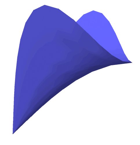
(a) The zero mean radius of curvature surface.

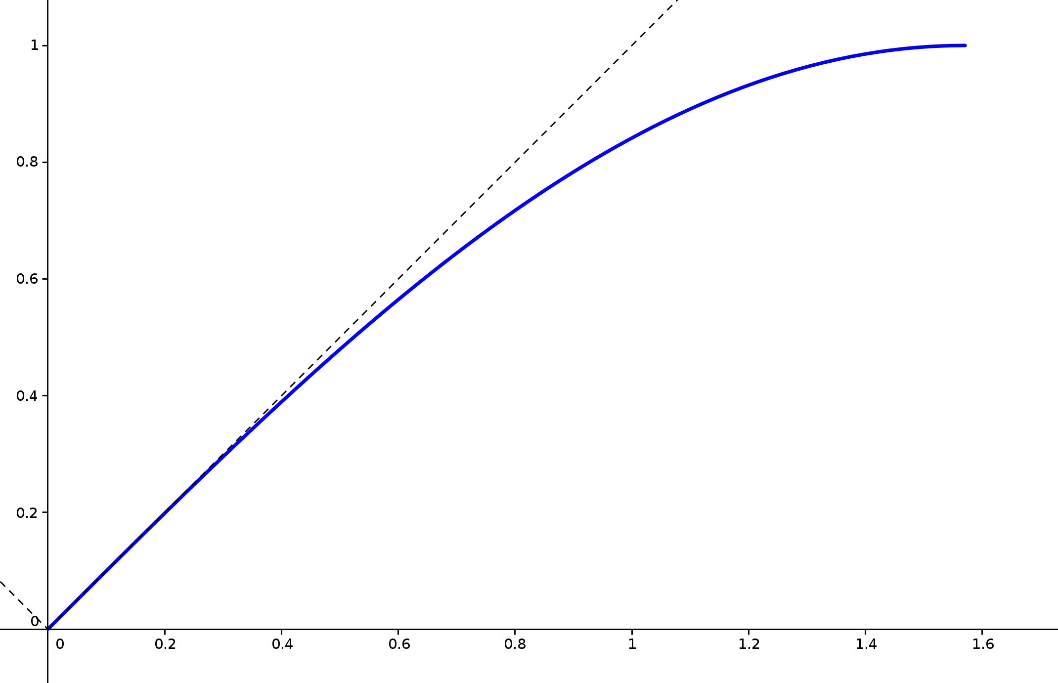
(b) The curve is the intersection of the surface with the $\{x_{2}=0\}$ plane. It can also be obtained from the function $h:{\mathbb{R}}^{+}\rightarrow{\mathbb{R}}$, $h(t)=\sinh(t)\arctan\left(\frac{1}{\sinh(t)}\right)-1$ and formula (26). Its radius of curvature is $\frac{-1}{\cosh(t)^{2}}$.

Figure 12: To Example 4.26.

4.6.2 Sovertkov condition for uniqueness

In [Sov81], the author proved the uniqueness among smooth solutions which do not grow too much. An easy observation gives that Sovertkov’s result holds as well for distribution solutions.

Theorem 4.27.

Let $\mu$ be a positive radon measure on $\mathbb{H}^{d}$ and let $\zeta:\partial\mathbb{H}^{d}\to\mathbb{R}$ be a function defined on the hyperbolic boundary at infinity. There is at most one continuous distribution solution $h$ to the equation (56) satisfying

$$\forall\theta,\quad\underset{\rho\rightarrow+\infty}{\mathrm{lim}}\frac{h(\rho,\mathbf{\theta})}{\cosh(\rho)}=\zeta(\theta).$$ (73)

By Lemma 2.22, the result above has a clear geometric meaning: two F-convex sets with the same first area measure are equal if for any null direction $\ell$ they have the same support plane at infinity directed by $\ell$. In particular, if $\zeta$ is continuous, the two convex sets must be contained in the future cone of a point.

Proof.

Let $h_{1},h_{2}\in\mathcal{D}^{\prime}(\mathbb{H}^{n})$ be two continuous functions satisfying (73) and

$$\Delta h_{1}-dh_{1}=\mu=\Delta h_{2}-dh_{2}$$

in $\mathcal{D}^{\prime}(\mathbb{H}^{n})$. Then, $h_{3}=h_{1}-h_{2}$ satisfies

$$\forall\theta,\quad\underset{\rho\rightarrow+\infty}{\mathrm{lim}}\frac{h_{3}(\rho,\mathbf{\theta})}{\cosh(\rho)}=0,$$

by the linearity of the equation

$$\frac{1}{d}\Delta h_{3}-h_{3}=0,$$ (74)

and by elliptic regularity $h_{3}\in C^{\infty}(\mathbb{H}^{n})$, [Aub98]. Hence we can proceed as in [Sov81] to prove that $h_{3}=0$. Namely, let $\varepsilon>0$ and define the smooth functions

$$h^{(\varepsilon)}_{\pm}(\rho,\mathbf{\theta}):=\varepsilon\left(\cosh(\rho)+1\right)\pm h_{3}(\rho,\mathbf{\theta}).$$

Both $h^{(\varepsilon)}_{\pm}$ satisfy

$$\underset{\rho\rightarrow+\infty}{\mathrm{lim}}h^{(\varepsilon)}_{\pm}(\rho,\mathbf{\theta})=\underset{\rho\rightarrow+\infty}{\mathrm{lim}}\left(\cosh(\rho)+1\right)\left(\varepsilon\pm\frac{h_{3}(\rho,\mathbf{\theta})}{\cosh(\rho)+1}\right)>0,$$

for all $\mathbf{\theta}$, and

$$\frac{1}{d}\Delta h^{(\varepsilon)}_{\pm}-h^{(\varepsilon)}_{\pm}=-\varepsilon d<0.$$

By the maximum principle we thus get that $h^{(\varepsilon)}_{\pm}$ are strictly positive for all $\varepsilon$, that is

$$|h_{3}(\rho,\mathbf{\theta})|<\varepsilon\left(\cosh(\rho)+1\right)$$

for all $\varepsilon>0$ and $(\rho,\mathbf{\theta})\in\mathbb{H}^{d}$. This proves the claim. ∎

4.6.3 Non-uniqueness

Reasoning as in the proof of Theorem 4.27, it is possible to get a characterization of non-unique solutions. In fact, let $h_{1}$ and $h_{2}$ be two distributions solutions to the equation (56) for some positive Radon measure $\mu$ on $\mathbb{H}^{d}$. Then $h=h_{1}-h_{2}$ satisfies the homogeneous equation (74) and is hence smooth by elliptic regularity. This elementary observation easily implies the following

Proposition 4.28.

Let $\mu\in\mathcal{R}(\mathbb{H}^{d})^{+}$ and let $h_{\mu}$ be the distribution solution to equation (56) defined in (57). If $h_{\mu}\in\mathcal{D}^{\prime}(\mathbb{H}^{d})\setminus C^{0}(\mathbb{H}^{d})$, then there exists no F-convex set $K$ with $\mu$ as first area measure.

Proof.

By contradiction, suppose such a convex $K$ exists. Then its restricted support function $h_{K}$ is a continuous solution to (56). But $h_{\mu}-h_{K}\in C^{\infty}(\mathbb{H}^{d})$ by elliptic regularity, and this gives us a contradiction. ∎

Example 4.29.

Let $\mu=\delta_{y}$ be the Dirac distribution at the point $y\in\mathbb{H}^{d}$. Then the solution to (62) proposed in (57) is

$$h_{\delta}(x)=G(x,y)\in D^{\prime}(\mathbb{H}^{d})\setminus C^{0}(\mathbb{H}^{d}).$$

Hence, by Proposition 4.28, there is no F-convex set with first area measure $\delta_{y}$. On the other hand, this result is not surprising, since by Section 4.6.1 we know that a continuous solution $h$ to $\frac{1}{d}\Delta h-h=\delta_{y}$ that is restriction to ${\mathbb{H}}^{d}$ of a convex function, has to be the restriction of a linear function on $\mathbb{H}^{d}\setminus\{y\}$, hence on all of $\mathbb{H}^{d}$ by continuity.

4.7 Proof of Theorem 1.1

The uniqueness is a consequence of Theorem 4.27 together with Lemma 2.23 (it will also follows from Corollary 5.2).

The first part of Theorem 1.1 follows from Theorem 4.10, the second from Proposition 4.17 and the third from Theorem 4.9.

4.8 The $d=1$ case

We specify here the analytical results of the previous section to the one dimensional setting, where an almost complete picture can be given. Actually, the first area measure is also the last area measure, so in $d=1$ there is a unique Christoffel–Minkowski problem. In fact in this case we have $\mathbb{H}^{1}=\mathbb{R}^{1}$ (see Subsection 2.15), and the first area measure is a positive Radon measure $\mu$ on $\mathbb{R}$. Accordingly, equation (62) reads

$$h^{\prime\prime}(t)-h(t)=\mu,\quad\textrm{in }\mathcal{D}^{\prime}(\mathbb{R})$$ (75)

in the sense of distributions, that is

$$\int_{-\infty}^{\infty}h(s)(f^{\prime\prime}(s)-f(s))\mathrm{d}s=\int_{-\infty}^{\infty}f(s)\mathrm{d}\mu(s),\quad\forall f\in C^{\infty}_{c}(\mathbb{R}).$$

Assume that $\mu\in\mathcal{R}^{+}(\mathbb{H}^{1})$, that is

$$\int_{-\infty}^{\infty}e^{-|t|}\mathrm{d}\mu(t)<\infty.$$ (76)

Reasoning as in the previous sections, we get that a particular solution to (75) takes the form

$$h_{\mu}(t)=-\int_{-\infty}^{\infty}\frac{e^{-|s-t|}}{2}\mathrm{d}\mu(s),$$

where the distribution $h_{\mu}\in\mathcal{D}^{\prime}(\mathbb{R})$ is defined by

$$(h_{\mu},f):=(\mu,h_{f})=-\int_{-\infty}^{\infty}\left(\int_{-\infty}^{\infty}\frac{e^{-|s-t|}}{2}f(s)\mathrm{d}s\right)\mathrm{d}\mu(t),\quad\forall f\in C^{\infty}_{c}(\mathbb{R}),$$

and is well-defined because of (76). In fact an integration by parts yields

$$({h_{\mu}}^{\prime\prime}-h_{\mu},f) =(h_{\mu},f^{\prime\prime}-f)=-\int_{-\infty}^{\infty}\left(\int_{-\infty}^{\infty}\frac{e^{-|s-t|}}{2}(f^{\prime\prime}(s)-f(s))\mathrm{d}s\right)\mathrm{d}\mu(t)=\int_{-\infty}^{\infty}f(t)\mathrm{d}\mu(t).$$

We note that, thanks to condition (76), even if the function $f:=-e^{-|s|}/2$ is not compactly supported, the convolution $h_{\mu}=f\ast\mu$ inherits the continuity property of $f$.
Considering also solutions to the homogeneous equation $h^{\prime\prime}=h$, we get that for $\mu\in\mathcal{R}^{+}(\mathbb{H}^{1})$ all solutions to equations (75) are continuous and can be written as

$$h_{\mu}(t)=-\int_{-\infty}^{\infty}\frac{e^{-|s-t|}}{2}\mathrm{d}\mu(s)+A\cosh(t)+B\sinh(t),\quad A,B\in\mathbb{R}.$$ (77)

When $\mu=\varphi(t)\mathrm{d}t$ for some $\varphi\in C^{0}(\mathbb{R})$, then assumption (76) can be skipped. In fact the general solution to equation

$$h^{\prime\prime}(t)-h(t)=\varphi(t)$$ (78)

can be also written in the form

$$h_{\varphi}=\int_{1}^{t}\sinh(t-s)\varphi(s)\mathrm{d}s+C\cosh(t)+D\sinh(t),\quad C,D\in\mathbb{R},$$ (79)

which makes sense for any continuous function $\varphi$ without growth assumption. We note that, when

$$\int_{-\infty}^{\infty}e^{-|t|}\varphi(t)\mathrm{d}t<\infty,$$

the expression in (79) and in (77) are the same up to set

$$A=C+\frac{1}{2}\int_{1}^{\infty}e^{-s}\varphi(s)\mathrm{d}s+\frac{1}{2}\int_{-\infty}^{1}e^{s}\varphi(s)\mathrm{d}s,$$

$$B=D+\frac{1}{2}\int_{1}^{\infty}e^{-s}\varphi(s)\mathrm{d}s-\frac{1}{2}\int_{-\infty}^{1}e^{s}\varphi(s)\mathrm{d}s.$$

Since the problem is one dimensional, equation (78) can be interpreted also as

$$\nabla^{2}h-gh=\varphi\geq 0$$

hence all the solutions given in (79) are automatically restrictions to $\mathbb{H}^{1}$ of convex functions on $\mathcal{F}$.

When $\mu\in\mathcal{R}(\mathbb{H}^{1})$ is a positive measure, one expects to get the same conclusion for solutions of (75), since, roughly speaking, $\nabla^{2}h-gh=\mu>0$ in the sense of distribution. To prove this, thanks to Lemma 2.53, it is enough to show that

$$h_{\mu}(t+\alpha)+h_{\mu}(t-\alpha)\geq 2\cosh(\alpha)h_{\mu}(t)$$

for all $t,\alpha\in\mathbb{R}$. We let $t$ be fixed, and since this latter is an even condition, we can assume without loss of generality that $\alpha>0$. Then, an explicit computation gives that

$$2\cosh(\alpha)h_{\mu}(t)-h_{\mu}(t+\alpha)-h_{\mu}(t-\alpha)=\int_{-\infty}^{\infty}\left[-\cosh(\alpha)e^{-|t-s|}+\frac{e^{-|t+\alpha-s|}}{2}+\frac{e^{-|t-\alpha-s|}}{2}\right]\mathrm{d}\mu(s)\leq 0,$$

since

$$\left[-\cosh(\alpha)e^{-|t-s|}+\frac{e^{-|t+\alpha-s|}}{2}+\frac{e^{-|t-\alpha-s|}}{2}\right]=\begin{cases}0,&\textrm{if }|t-s|\geq\alpha,\\ \sinh(|t-s|-\alpha)\leq 0,&\textrm{if }|t-s|<\alpha.\end{cases}$$

Example 4.30.

To end this section, we remark that here we get also an explicit expression for the Elementary example of Example 2.31 in the $d=1$ case. This is no more true in higher dimension, as we discussed in Example 4.13. In fact, in one dimension we have to consider a measure concentrated in a point, that is for instance $\mu=\delta_{0}$, the Dirac mass at the origin. Hence a special solution $h_{\delta_{0}}$ given by (77) is

$$h_{\delta_{0}}(t)=\frac{e^{-|t|}}{2},$$

which is the restriction to ${\mathbb{H}}^{1}$ of the $1$-homogeneous piecewise linear function $H$ on $\mathbb{R}^{2}$ defined as

$$H(x_{1},x_{2})=\begin{cases}x_{2}+x_{1},&\textrm{if }x_{1}<0\\ x_{2}-x_{1},&\textrm{if }x_{1}\geq 0.\end{cases}$$

5 Quasi–Fuchsian solutions

5.1 Uniqueness of solution

We start this section with the simple proof of the fact that the solution to (65) is unique in the quasi-Fuchsian case. Actually, it can be shown that this result follows from Theorem 4.27, see Remark 2.19.

Proposition 5.1.

Given $\bar{\mu}\in\mathcal{R}({\mathbb{H}^{d}/\Gamma})$, the equation (65) has a unique solution $\bar{h}_{\bar{\mu}}$ in the sense of distributions, whose explicit expression is given in (68).

Proof.

Let $\bar{T}_{1},\bar{T}_{2}\in\mathcal{D}^{\prime}({\mathbb{H}^{d}/\Gamma})$ be two solution of $\eqref{eq_dist_Gamma}$. Choose $\bar{\eta}\in C^{\infty}({\mathbb{H}^{d}/\Gamma})$ and let $\bar{h}_{\bar{\eta}}\in C^{\infty}({\mathbb{H}^{d}/\Gamma})$ be a solution to $\frac{1}{d}\Delta\bar{h}_{\bar{\eta}}-\bar{h}_{\bar{\eta}}=\bar{\eta}$, which exists thanks to Theorem 4.9. Then

$$(\bar{T}_{1},\bar{\eta})=(\bar{T}_{1},\frac{1}{d}\Delta\bar{h}_{\bar{\eta}}-\bar{h}_{\bar{\eta}})=(\frac{1}{d}\Delta\bar{T}_{1}-\bar{T}_{1},\bar{h}_{\bar{\eta}})=(\bar{\mu},\bar{h}_{\bar{\eta}})=(\frac{1}{d}\Delta\bar{T}_{2}-\bar{T}_{2},\bar{h}_{\bar{\eta}})=(\bar{T}_{2},\frac{1}{d}\Delta\bar{h}_{\bar{\eta}}-\bar{h}_{\bar{\eta}})=(\bar{T}_{2},\bar{\eta}).$$

Since $\bar{\eta}$ is arbitrary, this proves that $\bar{T}_{1}=\bar{T}_{2}$ in the sense of distributions. ∎

Corollary 5.2.

Let $\tau$ be a cocycle and let $h$ and $h^{\prime}$ be two $\tau$-equivariant maps such that $S_{1}(h)=S_{1}(h^{\prime})$. Then $h=h^{\prime}$. In particular there exists at most one $\tau$-F-convex set with a given first area measure.

Proof.

By linearity, $S_{1}(h-h^{\prime})=0$, but $h-h^{\prime}$ is $\Gamma$-invariant, so by Proposition 5.1, $h=h^{\prime}$. The second part follows by considering support functions for $h$ and $h^{\prime}$. ∎

5.2 The $\tau$-hedgehog of zero curvature

Lemma 5.3.

For any $\tau\in Z^{1}(\Gamma,{\mathbb{R}}^{d+1})$, there exists a unique $C^{\infty}$ $\tau$-hedgehog $\lambda_{\tau}$ with $S_{1}(\lambda_{\tau})=0$. It is the support function of a convex set if and only if $\tau$ is a coboundary.

In the Fuchsian case ($\tau=0$), $\lambda_{\tau}$ is the origin.

Proof.

Let $h$ be a $\tau$-equivariant map. By Theorem 4.10 there exits a $\Gamma$-invariant function $h_{0}$ such that $S_{1}(h_{0})=S_{1}(h)$ in the sense of distribution ($h_{0}$ is a continuous function by the arguments of Subsubsection 4.6.3). Let us define $\lambda_{\tau}=h-h_{0}$. It has the following properties:

• $\lambda_{\tau}$ is unique: by Corollary 5.2. In particular, it is well-defined in the sense that is depends only on $\tau$.

• $S_{1}(\lambda_{\tau})=0$: by construction.

• $\lambda_{\tau}$ is $C^{\infty}$: by the preceding item and elliptic regularity.

• If $\tau$ is a coboundary, with the notations of (v) of Lemma 2.3, $S_{1}(H)=S_{1}(H_{0})$, $H-H_{0}=\langle\cdot,v\rangle_{-}$ and this is the $1$-extension of $\lambda_{\tau}$.

• If $H-H_{0}$ is convex, as $H$ and $H_{0}$ have the same area measure, by Subsubsection 4.6.1, $H$ and $H_{0}$ differ by the restriction to ${\mathcal{F}}$ of a linear form. So $\tau$ is a coboundary.

• $\lambda_{\tau}$ is $\tau$-equivariant by construction.

∎

Remark 5.4 (Formal eigenfunctions of the hyperbolic Laplacian).

Let us denote by $E(d)$ the space of formal eigenfunctions of the Laplacian of ${\mathbb{H}}^{d}$ for the eigenvalue $d$. For any $\tau\in Z^{1}(\Gamma,{\mathbb{R}}^{d+1})$, $\lambda_{\tau}$ belongs to $E(d)$ (note that its $1$-extension is a formal eigenfunction of the wave operator). Actually this correspondence is a linear injection.

Lemma 5.5.

The map $\lambda:\tau\mapsto\lambda_{\tau}$ from $Z^{1}(\Gamma,{\mathbb{R}}^{d+1})$ to $E(d)$ is an injective linear map.

The image of $B^{1}(\Gamma,{\mathbb{R}}^{d+1})$ is the set of the restrictions to ${\mathbb{H}}^{d}$ of linear forms of ${\mathbb{R}}^{d+1}$.

Proof.

We already know that the image of $Z^{1}$ belongs to $E(d)$.

$\lambda$ is injective: Let $\tau^{\prime}\in Z^{1}$. If $\lambda(\tau)=\lambda(\tau^{\prime})$, then there exists a $\tau$-equivariant function $h$, a $\tau^{\prime}$-equivariant function $h^{\prime}$ and $\Gamma$ invariant functions $h_{0}$ and $h_{0}^{\prime}$ with $h^{\prime}-h_{0}^{\prime}=h-h_{0}$ i.e. $h^{\prime}+h_{0}=h+h_{0}$. The right hand side is a $\tau$-equivariant function and the left hand side is a $\tau^{\prime}$-equivariant function. The result follows from Lemma 2.3.

$\lambda$ is linear: with the preceding notations and $\alpha$ a real number, from Lemma 2.3, $\alpha h+h^{\prime}$ is $(\alpha\tau+\tau^{\prime})$-equivariant. On one hand, $\alpha(h-h_{0})+h^{\prime}-h_{0}^{\prime}$ is equal to $\alpha\lambda_{\tau}+\lambda_{\tau^{\prime}}$. On the other hand, $S_{1}(\alpha h+h^{\prime})=S_{1}(\alpha h_{0}+h_{0}^{\prime})$ hence $\alpha h+h^{\prime}-\alpha h_{0}+h_{0}^{\prime}$ is equal to $\lambda_{\alpha\tau+\tau^{\prime}}$.

$\lambda(B^{1})$: we already know that the image is made of restriction of linear forms. The result follows because $\lambda$ is linear and $B^{1}$ has dimension $d+1$. ∎

Remark 5.6 (Slicing by constant mean radius of curvature).

From Lemma 2.55, we get two positive constants $c_{1}$ and $c_{2}$ such that, for any positive $c$, $\lambda_{\tau}-c_{1}-c$ is a slicing of an unbounded part of the $\tau$-F-regular domain $\Omega^{+}_{\tau}$ by smooth convex Cauchy surfaces with constant mean radius of curvature. In the same way, $\lambda_{\tau}+c_{2}+c$ is a slicing of an unbounded part of the $\tau$-P-convex domain $\Omega^{-}_{\tau}$ by smooth convex Cauchy surfaces with constant mean radius of curvature. Taking negative $c$, the slicing can be extended, going outside of $\Omega^{+}_{\tau}\cup\Omega^{-}_{\tau}$, and the slices are $\tau$-hedgehogs.

Remark 5.7 (Quasi-Fuchsian Christoffel problem).

The uniqueness part of the problem is solved by Corollary 5.2. Given a $\Gamma$-invariant measure $\mu$, Theorem 4.9 gives the (unique) $\Gamma$-invariant solution $h_{0}$ of $S_{1}(h_{0})=\mu$. So $h:=h_{0}+\lambda_{\tau}$ is the unique $\tau$-equivariant solution of $S_{1}(h)=\mu$, in the sense of distribution. To know when $h$ is the support function of a $\tau$-F-convex set, one has to use Proposition 4.17.

Remark 5.8 (Relations with Codazzi tensors).

A Codazzi tensor (here on a hyperbolic surface $S$) is a self-adjoint $(0,2)$-tensor which satisfies the Codazzi equation. For example, for any smooth function $u$ on $S$, $\mathrm{Hess}u-u\mathrm{Id}$ is a Codazzi tensor. If $S$ is compact, a group isomorphism $\Phi$ between the space of traceless Codazzi tensor and $H^{1}(\Gamma,{\mathbb{R}}^{3})$ ($\Gamma=\pi_{1}(S)$) is constructed in [BS]: Let $\tilde{b}$ be the lifting of $b$ to ${\mathbb{H}}^{2}$. From a result of [OS83], there exists a smooth map $h:{\mathbb{H}}^{2}\rightarrow R$ with $\tilde{b}=\mathrm{Hess}h-h\mathrm{Id}$. It can be checked that $\tilde{b}$ is $\tau$-equivariant, for a $\tau\in Z^{1}(\Gamma,{\mathbb{R}}^{3})$. Then define $\Phi(b)=\tau$. Lemma 5.3 says that $\Phi$ is surjective: for any $\tau$, $\mathrm{Hess}\lambda_{\tau}-\lambda_{\tau}\mathrm{Id}$ is a traceless Codazzi operator on ${\mathbb{H}}^{d}/\Gamma$.

5.3 Mean width of flat GHCM spacetimes

Let $h$ be a $\tau$-equivariant map. The map $h-\lambda_{\tau}$ is $\Gamma$-invariant, and $S_{1}(h)=S_{1}(h-\lambda_{\tau})$. With the notations of Subsection 4.3 together with the definition of the action given in (39), $\forall f\in C^{\infty}({\mathbb{H}}^{d}/\Gamma)$, the action of the first area measure on ${\mathbb{H}}^{d}/\Gamma$ writes as

$$(\overline{S}_{1}(\overline{h-\lambda_{\tau}}),f)=\int_{{\mathbb{H}}^{d}/\Gamma}(\overline{h-\lambda_{\tau}})\left(\frac{1}{d}\Delta-1\right)f.$$

Let $h$ be the support function of a $\tau$-F-convex set $K$. The Radon measure $S_{1}(K,\cdot)$ is $\Gamma$ invariant, so for any fundamental domain $\omega$ for the action of $\Gamma$, we can define the total first area measure of $K$ by $\overline{S}_{1}(K):=S_{1}(K,\omega)$. Actually, $S_{1}(K,\cdot)$ gives a Radon measure $\overline{S}_{1}(K,\cdot)$ on ${\mathbb{H}}^{d}/\Gamma$, and $\overline{S}_{1}(K)=\overline{S}_{1}(K,{\mathbb{H}}^{d}/\Gamma)$. By setting $f=1$ in the above formula, we obtain (compare with Remark 3.16)

$$\overline{S}_{1}(K)=-\int_{{\mathbb{H}}^{d}/\Gamma}\overline{h-\lambda_{\tau}}.$$ (80)

Let us consider a $\tau$-F-regular domain $\Omega^{+}_{\tau}$ with simplicial singularity (see Subsection 2.8). In this case, the total mass of the measured geodesic stratification on ${\mathbb{H}}^{d}/\Gamma$ is equal to $\overline{S}_{1}(\Omega^{+}_{\tau})$ (see Remark 3.23).

From the given cocycle $\tau$, one also get a $\tau$-P-regular domain $\Omega_{\tau}^{-}$ (it is given for example by the symmetry with respect to the origin of the F-convex domain $\Omega_{-\tau}$). The meaning of $\overline{S}_{1}(\Omega_{\tau}^{-})$ is clear. Let us denote by $h^{+}_{\tau}$ the support function of $\Omega^{+}_{\tau}$ and by $h^{-}_{\tau}$ the support function of $\Omega^{-}_{-\tau}$, which is a $(-\tau)$-equivariant map. Moreover $-\lambda_{\tau}=\lambda_{-\tau}$, so using (80) and the equation above,

$$\overline{S}_{1}(\Omega_{\tau}^{-})+\overline{S}_{1}(\Omega_{\tau}^{+})=-\int_{{\mathbb{H}}^{d}/\Gamma}\overline{h_{\tau}^{+}+h_{\tau}^{-}}.$$

This last formula has the following geometric meaning. Let $\eta\in{\mathcal{F}}$, and $-1:{\mathbb{R}}^{d}\rightarrow{\mathbb{R}}^{d},x\mapsto-x$. Then $h^{-}_{\tau}\circ-1$ is the support function (defined on $-{\mathcal{F}}$) of $\Omega_{\tau}^{-}$. So $(h_{\tau}^{+}+h_{\tau}^{-})(\eta)$ is the “distance” between the support planes of $\Omega_{\tau}^{+}$ and $\Omega_{\tau}^{+}$ orthogonal to $\eta$ ($(h_{\tau}^{+}+h_{\tau}^{-})(\eta)<0$ says that the respective half-spaces are disjoint). Hence $-\int_{{\mathbb{H}}^{d}/\Gamma}\overline{h_{\tau}^{+}+h_{\tau}^{-}}$ divided by the volume of ${\mathbb{H}}^{d}/\Gamma$ can be called the mean width of the flat spacetime $(\Omega_{\tau}^{+}\cup\Omega_{\tau}^{-})/\Gamma_{\tau}$. We get that this mean width is determined by the total mass of the measured geodesic stratifications defining the spacetime. In the Fuchsian case $\tau=0$, the mean width is null.

References

- [ABB+07] L. Andersson, T. Barbot, R. Benedetti, F. Bonsante, W. Goldman, F. Labourie, K. Scannell, and J.-M. Schlenker. Notes on: “Lorentz spacetimes of constant curvature” [Geom. Dedicata 126 (2007), 3–45; mr2328921] by G. Mess. Geom. Dedicata, 126:47–70, 2007.
- [ABBZ12] L. Andersson, T. Barbot, F. Béguin, and A. Zeghib. Cosmological time versus CMC time in spacetimes of constant curvature. Asian J. Math., 16(1):37–87, 2012.
- [Ale37] A. D. Alexandrov. On the theory of mixed volumes I. Mat. Sbornik, 2(5):947–972, 1937. (Russian. Translated in [Ale96]).
- [Ale96] A. D. Alexandrov. Selected works. Part I, volume 4 of Classics of Soviet Mathematics. Gordon and Breach Publishers, Amsterdam, 1996. Selected scientific papers, Translated from the Russian by P. S. V. Naidu, Edited and with a preface by Yu. G. Reshetnyak and S. S. Kutateladze.
- [Ale12] A. D. Alexandrov. On the surfaces representable as difference of convex functions [translation of mr0048059]. Sib. Èlektron. Mat. Izv., 9:360–376, 2012.
- [Aub98] T. Aubin. Some nonlinear problems in Riemannian geometry. Springer Monographs in Mathematics. Springer-Verlag, Berlin, 1998.
- [Bar05] T. Barbot. Globally hyperbolic flat space-times. J. Geom. Phys., 53(2):123–165, 2005.
- [BB09] R. Benedetti and F. Bonsante. Canonical Wick rotations in 3-dimensional gravity. Mem. Amer. Math. Soc., 198(926):viii+164, 2009.
- [BBZ11] T. Barbot, F. Béguin, and A. Zeghib. Prescribing Gauss curvature of surfaces in 3-dimensional spacetimes: application to the Minkowski problem in the Minkowski space. Ann. Inst. Fourier (Grenoble), 61(2):511–591, 2011.
- [Ber69] C. Berg. Corps convexes et potentiels sphériques. Mat.-Fys. Medd. Danske Vid. Selsk., 37(6):64 pp. (1969), 1969.
- [Ber14] J. Bertrand. Prescription of Gauss curvature on compact hyperbolic orbifolds. Discrete Contin. Dyn. Syst., 34(4):1269–1284, 2014.
- [BF14] F. Bonsante and F. Fillastre. The equivariant Minkowski problem in Minkowski space, arXiv:1405.4376 2014.
- [BMS13] F. Bonsante, C. Meusburger, and J.-M. Schlenker. Recovering the geometry of a flat spacetime from background radiation. Annales Henri Poincaré, 15:9 (2014), 1733–1799.
- [Bon05] F. Bonsante. Flat spacetimes with compact hyperbolic Cauchy surfaces. J. Differential Geom., 69(3):441–521, 2005.
- [BS] F. Bonsante and A. Seppi. On Codazzi tensors on a hyperbolic surface and flat Lorentzian geometry, arXiv:1501.04922 2015.
- [CBC+11] F. Catoni, D. Boccaletti, R. Cannata, V. Catoni, and P. Zampetti. Geometry of Minkowski space-time. Springer Briefs in Physics. Springer, Heidelberg, 2011.
- [Far96] F. T. Farrell. Lectures on surgical methods in rigidity. Published for the Tata Institute of Fundamental Research, Bombay, 1996.
- [FI] F. Fillastre and I. Izmestiev. Shapes of polyhedra, mixed volumes, and hyperbolic geometry, arXiv:1310.1560 2013.
- [Fil13] F. Fillastre. Fuchsian convex bodies: basics of Brunn-Minkowski theory. Geom. Funct. Anal., 23(1):295–333, 2013.
- [Fir67] W. J. Firey. The determination of convex bodies from their mean radius of curvature functions. Mathematika, 14:1–13, 1967.
- [Fir68] W. J. Firey. Christoffel’s problem for general convex bodies. Mathematika, 15:7–21, 1968.
- [Fir70] W. J. Firey. Local behaviour of area functions of convex bodies. Pacific J. Math., 35:345–357, 1970.
- [Fir74] W. J. Firey. Approximating convex bodies by algebraic ones. Arch. Math. (Basel), 25:424–425, 1974.
- [Fir81] W. J. Firey. Subsequent work on Christoffel’s problem about determining a surface from local measurements. In E. B. Christoffel (Aachen/Monschau, 1979), pages 721–723. Birkhäuser, Basel, 1981.
- [FJ38] W. Fenchel and B. Jessen. Mengenfunktionen und konvexe körper. Danske Videnks. Selsk. Math.-fys. Medd., 16(3), 1938.
- [Gho02] M. Ghomi. The problem of optimal smoothing for convex functions. Proc. Amer. Math. Soc., 130(8):2255–2259 (electronic), 2002.
- [GKR68] D. Gale, V. Klee, and R. T. Rockafellar. Convex functions on convex polytopes. Proc. Amer. Math. Soc., 19:867–873, 1968.
- [GLL12] P. Guan, J. Li, and Y. Li. Hypersurfaces of prescribed curvature measure. Duke Math. J., 161(10):1927–1942, 2012.
- [GLM06] P. Guan, C. Lin, and X. Ma. The Christoffel-Minkowski problem. II. Weingarten curvature equations. Chinese Ann. Math. Ser. B, 27(6):595–614, 2006.
- [GM03] P. Guan and X.-N. Ma. The Christoffel-Minkowski problem. I. Convexity of solutions of a Hessian equation. Invent. Math., 151(3):553–577, 2003.
- [GMZ06] P. Guan, X.-N. Ma, and F. Zhou. The Christofel-Minkowski problem. III. Existence and convexity of admissible solutions. Comm. Pure Appl. Math., 59(9):1352–1376, 2006.
- [GYY11] P. Goodey, V. Yaskin, and M. Yaskina. A Fourier transform approach to Christoffel’s problem. Trans. Amer. Math. Soc., 363(12):6351–6384, 2011.
- [GZ99] E. Grinberg and G. Zhang. Convolutions, transforms, and convex bodies. Proc. London Math. Soc. (3), 78(1):77–115, 1999.
- [Har59] P. Hartman. On functions representable as a difference of convex functions. Pacific J. Math., 9:707–713, 1959.
- [Hel59] S. Helgason. Differential operators on homogenous spaces. Acta Math., 102:239–299, 1959.
- [Hel62] S. Helgason. Differential geometry and symmetric spaces. Pure and Applied Mathematics, Vol. XII. Academic Press, New York, 1962.
- [Hör07] L. Hörmander. Notions of convexity. Modern Birkhäuser Classics. Birkhäuser Boston Inc., Boston, MA, 2007. Reprint of the 1994 edition.
- [HU85] J.-B. Hiriart-Urruty. Generalized differentiability, duality and optimization for problems dealing with differences of convex functions. In Convexity and duality in optimization (Groningen, 1984), volume 256 of Lecture Notes in Econom. and Math. Systems, pages 37–70. Springer, Berlin, 1985.
- [HUL93] J.-B. Hiriart-Urruty and C. Lemaréchal. Convex analysis and minimization algorithms. I, volume 305 of Grundlehren der Mathematischen Wissenschaften [Fundamental Principles of Mathematical Sciences]. Springer-Verlag, Berlin, 1993. Fundamentals.
- [Kal74] M. Kallay. Reconstruction of a plane convex body from the curvature of its boundary. Israel J. Math., 17:149–161, 1974.
- [Kam09] J. Kampf. On weighted parallel volumes. Beiträge Algebra Geom., 50(2):495–519, 2009.
- [LdLSdL06] L. Lopes de Lima and J. H. Soares de Lira. The Christoffel problem in Lorentzian geometry. J. Inst. Math. Jussieu, 5(1):81–99, 2006.
- [LLR88] R. Langevin, G. Levitt, and H. Rosenberg. Hérissons et multihérissons (enveloppes parametrées par leur application de Gauss). In Singularities (Warsaw, 1985), volume 20 of Banach Center Publ., pages 245–253. PWN, Warsaw, 1988.
- [Mar07] A. Marden. Outer circles. Cambridge University Press, Cambridge, 2007. An introduction to hyperbolic 3-manifolds.
- [Mat95] P. Mattila. Geometry of sets and measures in Euclidean spaces, volume 44 of Cambridge Studies in Advanced Mathematics. Cambridge University Press, Cambridge, 1995. Fractals and rectifiability.
- [Mes07] G. Mess. Lorentz spacetimes of constant curvature. Geom. Dedicata, 126:3–45, 2007. Written in 1990.
- [NP91] M. Näätänen and R. C. Penner. The convex hull construction for compact surfaces and the Dirichlet polygon. Bull. London Math. Soc., 23(6):568–574, 1991.
- [Oli92] V. Oliker. Generalized convex bodies and generalized envelopes. In Geometric analysis (Philadelphia, PA, 1991), volume 140 of Contemp. Math., pages 105–113. Amer. Math. Soc., Providence, RI, 1992.
- [O’N83] B. O’Neill. Semi-Riemannian geometry, volume 103 of Pure and Applied Mathematics. Academic Press Inc. [Harcourt Brace Jovanovich Publishers], New York, 1983. With applications to relativity.
- [OS83] V. I. Oliker and U. Simon. Codazzi tensors and equations of Monge-Ampère type on compact manifolds of constant sectional curvature. J. Reine Angew. Math., 342:35–65, 1983.
- [Pog53] A. V. Pogorelov. On existence of a convex surface with a given sum of the principal radii of curvature. Uspehi Matem. Nauk (N.S.), 8(3(55)):127–130, 1953.
- [Pog73] A. V. Pogorelov. Extrinsic geometry of convex surfaces. American Mathematical Society, Providence, R.I., 1973. Translated from the Russian by Israel Program for Scientific Translations, Translations of Mathematical Monographs, Vol. 35.
- [Rat06] J. Ratcliffe. Foundations of hyperbolic manifolds, volume 149 of Graduate Texts in Mathematics. Springer, New York, second edition, 2006.
- [Roc97] T. Rockafellar. Convex analysis. Princeton Landmarks in Mathematics. Princeton University Press, Princeton, NJ, 1997. Reprint of the 1970 original, Princeton Paperbacks.
- [Sch77] R. Schneider. Das Christoffel-Problem für Polytope. Geometriae Dedicata, 6(1):81–85, 1977.
- [Sch93a] R. Schneider. Convex bodies: the Brunn-Minkowski theory, volume 44 of Encyclopedia of Mathematics and its Applications. Cambridge University Press, Cambridge, 1993.
- [Sch93b] L. Schwartz. Analyse. IV, volume 45 of Collection Enseignement des Sciences [Collection: The Teaching of Science]. Hermann, Paris, 1993. Applications à la théorie de la mesure.
- [Sov81] P. I. Sovertkov. The Christoffel problem in a pseudo-Euclidean space . Mat. Zametki, 30(5):737–747, 797, 1981.
- [Sov83] P. I. Sovertkov. The generalized Christoffel problem in a pseudo-Euclidean space . Izv. Vyssh. Uchebn. Zaved. Mat., (6):64–67, 1983.
- [Spi79] M. Spivak. A comprehensive introduction to differential geometry. Vol. II. Publish or Perish Inc., Wilmington, Del., second edition, 1979.
- [STW04] W. Sheng, N. Trudinger, and X.-J. Wang. Convex hypersurfaces of prescribed Weingarten curvatures. Comm. Anal. Geom., 12(1-2):213–232, 2004.
- [Tao10] T. Tao. An epsilon of room, I: real analysis, volume 117 of Graduate Studies in Mathematics. American Mathematical Society, Providence, RI, 2010. Pages from year three of a mathematical blog.
- [Thu02] W. P. Thurston. The geometry and topology of three-manifolds. 2002. Electronic version 1.1, http://library.msri.org/books/gt3m/.
- [Ves87] L. Veselý. A short proof of a theorem on compositions of d.c. mappings. Proc. Amer. Math. Soc., 101(4):685–686, 1987.
- [Yag79] I. M. Yaglom. A simple non-Euclidean geometry and its physical basis. Springer-Verlag, New York, 1979. An elementary account of Galilean geometry and the Galilean principle of relativity, Heidelberg Science Library, Translated from the Russian by Abe Shenitzer, With the editorial assistance of Basil Gordon.
- [Zel70] J. S. Zelver. The integro-geometric tangent measures of Euclidean n-space. PhD thesis, Oregon State University, 1970.