Quantum transport equations for low-dimensional multiband electronic systems. I

Abstract

A systematic method of calculating the dynamical conductivity tensor in a general multiband electronic model with strong boson-mediated electron-electron interactions is described. The theory is based on the exact semiclassical expression for the coupling between valence electrons and electromagnetic fields and on the self-consistent Bethe–Salpeter equations for the electron-hole propagators. The general diagrammatic perturbation expressions for the intraband and interband single-particle conductivity are determined. The relations between the intraband Bethe–Salpeter equation, the quantum transport equation and the ordinary transport equation are briefly discussed within the memory-function approximation. The effects of the Lorentz dipole-dipole interactions on the dynamical conductivity of low-dimensional $sp_{\alpha}$ models are described in the same approximation. Such formalism proves useful in studies of different (pseudo)gapped states of quasi-one-dimensional systems with the metal-to-insulator phase transitions and can be easily extended to underdoped two-dimensional high-$T_{c}$ superconductors.

I Introduction

The ab initio band structure calculations of strongly-interacting low-dimensional (quasi-one-dimensional (Q1D) or two-dimensional (2D)) systems (high-$T_{c}$ superconductor YBa₂Cu₃O_7-x as well as charge-density-wave (CDW) systems K_0.3MoO₃ and BaVS₃ being examples Massidda87 ; Whangbo86 ; Mattheiss95 ) usually reveal several bands in the vicinity of the Fermi level that are, in the leading approximation, decoupled from the rest of the band structure. In the tight-binding approximation, the bare dispersions of such a multiband model are well understood in terms of the strong hybridization among several properly chosen orbitals per unit cell, while the hybridization with the other electronic levels is neglected. Emery87 The bare single-particle tight-binding Hamiltonian is thus taken to include commensurate/incommensurate CDW or SDW (spin-density wave) average fields and several first-neighbour bond energies. In the two-particle Hamiltonian one usually retains the long-range Coulomb interactions, the largest local (Hubbard) interactions together with the most important short-range interactions. Associated with different terms in the single-particle Hamiltonian are fluctuations in the charge and spin densities on different orbitals in the unit cell and on the corresponding bonds. All these ingredients make strongly-interacting multiband electronic problems extremely complicated.

To explain most of experimental results on typical single-band systems, it usually suffices to describe properly the coupling between ${\bf q}\approx 0$ monopole charge fluctuations and external electromagnetic (EM) fields and combine this coupling Hamiltonian with the ordinary transport equations. Pines89 ; Ziman72 However, in multiband electronic systems, even in the cases when only one band intersects the Fermi level, the analysis is considerably more complicated. Not only the interband physics but also the intraband physics depends drastically on both single-particle and two-particle parameters of the Hamiltonian and are affected differently by various types of fluctuations. Therefore, to understand the results of transport measurements Ando04 ; Forro00 and reflectivity measurements Uchida91 ; Degiorgi91 ; Kezsmarki06 of multiband electronic systems in detail, we describe the ${\bf q}\approx 0$ multipolar fluctuations in the dynamical conductivity tensor in a way consistent with the results of experimental methods which probe charge and spin fluctuations which presumably occur at finite wave vectors Sugai03 ; Takigawa91 . The ${\bf q}\approx 0$ charge-charge correlation function is thus just one of several equally important correlation functions defined in terms of symmetrized intraband and interband charge and spin fluctuations. Common to all these correlation functions is a complicated structure of the intraband and interband electron-hole propagators. Therefore, to understand the contribution of different types of fluctuations to these correlation functions, in particular to the dynamical conductivity, we must first find the solution to quite general Bethe–Salpeter equations for the electron-hole propagators and then combine the result with the very definition of the response function under consideration. This question, which is of great importance in studies of strongly-interacting low-dimensional systems, is in the focus of the present analysis.

In this article, we thus present a general response theory which uses both an essentially exact semiclassical description of the coupling between valence electrons and external EM fields Landau95 ; Kupcic09b and a quite general description of the intraband and interband charge fluctuations Barisic90 ; Kupcic07 . The result is the current-dipole Kubo formula for the dynamical conductivity, Kubo95 with the structure of the intraband electron-hole propagators determined by means of the quantum transport equation (i.e., the intraband Bethe–Salpeter equation). To emphasize the connection between the present theory and the ordinary transport theory, Pines89 ; Ziman72 ; Eliashberg62 ; Abrikosov88 ; Vollhardt80 we determine the explicit form of the intraband conductivity in the memory-function approximation. Gotze72 ; Giamarchi91 ; Kupcic04 We also find the structure of the interband conductivity in both cases, with real and with purely imaginary interband dipole vertices, to show in which way the Lorentz local field corrections Adler62 ; Wieser62 ; Zupanovic96 affect the dynamical conductivity of interacting low-dimensional systems.

The article is organized as follows. To make the reading of the article easier, we give in section 2 an overview of the results. Then in section 3 the notation is introduced to describe electrons and boson modes in a general multiband electronic model with boson-mediated electron-electron interactions. A complementary multiband electronic model with nonretarded electron-electron interactions will be studied in a separate article KupcicUP which is focused on the commensurability effects in the single-particle conductivity tensor.

Starting with the quantum electrodynamical description of the interaction between valence electrons and external EM fields, we derive the exact semiclassical form of the electron-EM field coupling Hamiltonian in section 4. In section 5 we define the dynamical conductivity tensor and briefly discuss the relaxation-time approximation. Section 6 gives the structure of the self-consistent Bethe–Salpeter equations for the dipole vertex functions and for the related auxiliary electron-hole propagators (to be defined latter) in a general multiband case. We show the equivalence of the Bethe–Salpeter equation for the auxiliary intraband electron-hole propagators and the quantum transport equation. The generalized Drude formula is derived from the quantum transport equation by using the memory-function approximation. The bare interband conductivity is considered in section 7 and the related local field effects in section 8. Section 9 contains the concluding remarks.

II Overview of results

Before discussing the details of the dynamical conductivity model proposed in this article, we present an overview of the results. In this way principal physical messages of the present work are separated from the technical details.

We are interested here in a general low-dimensional model with multiple electronic bands in the presence of boson-mediated electron-electron interactions. The single-particle part of the total Hamiltonian is assumed to be exactly solvable. The Bloch energies $\varepsilon_{L}({\bf k})$ in the band labeled by the band index $L$ and all relevant bare vertex functions (the dipole vertices $P_{\alpha}^{LL^{\prime}}({\bf k},{\bf k}^{\prime})$, for example) are thus taken as known functions. To study the influence of the boson-mediated electron-electron interactions on single-electron propagators ${\cal G}_{L}({\bf k},{\rm i}\omega_{n})$ and, in addition, on different electron-hole propagators encountered in the response functions of interest, we use high-order diagrammatic perturbation theory of the metallic state, as usual in investigations of low-dimensional electronic systems. Abrikosov75 ; Dzyaloshinskii73

The electron-hole propagators are associated with the dispersive, undamped bosons which can either correspond to the external degrees of freedom coupled to electrons/holes or the internal degrees of freedom built of the electron-hole excitations at finite values of q. In sections 6–8, the emphasis is on the acoustic and Raman-active and infrared-active optical phonons. The scattering by phase and amplitude phonon modes of the common Peierls CDW model will be studied in detail within the microscopic Lee–Rice–Anderson model in the accompanying article KupcicJPCM (to be referred to as Article II).

Figure 1: The Dyson equation (1) for electron Green’s functions. $L$ is the electron band index and $\nu$ is the boson branch index. The black circle and the big gray circle represent, respectively, the bare and the renormalized electron-boson vertex. Here and herafter, the tiny and bold solid (dashed) lines are the bare and renormalized electron (boson) propagators.

In high-order perturbation theory, the electron Green’s function ${\cal G}_{L}({\bf k},{\rm i}\omega_{n})$ satisfies the Dyson equation Fetter71 ; Abrikosov75 ; Mahan90

$$\big{[}{\rm i}\hbar\omega_{n}-\varepsilon_{L}({\bf k})+\mu-\hbar\Sigma_{L}({\bf k},{\rm i}\omega_{n})\big{]}{\cal G}_{L}({\bf k},{\rm i}\omega_{n})=\hbar,$$ (1)

where $\Sigma_{L}({\bf k},{\rm i}\omega_{n})$ is the self-energy function of the electron (see figure 1). In this case $\Sigma_{L}({\bf k},{\rm i}\omega_{n})$ is a function of ${\cal G}_{L}({\bf k},{\rm i}\omega_{n})$, resulting in a system of two coupled equations. A strong reduction of the quasi-particle pole weight in ${\cal G}_{L}({\bf k},{\rm i}\omega_{n})$ at the Fermi level is predicted by different strictly 1D theories Dzyaloshinskii73 ; Solyom79 ; Giamarchi04 and observed in angle-resolved photoemission spectroscopy (ARPES) experiments on Q1D systems Vescoli00 ; Mitrovic07 . In this article we present a systematic method of calculating the dynamical conductivity tensor in interacting low-dimensional systems which is consistent with the described treatment of the single-electron Green’s functions ${\cal G}_{L}({\bf k},{\rm i}\omega_{n})$.

II.1 Electron coupling to EM fields

In semiclassical electrodynamics applied to a general exactly solvable single-particle problem with multiple electronic bands, the electric component of the EM field parallel to the cartesian axis $\alpha$, $E_{\alpha}({\bf q})$, couples to the currents of free charges and to the dipole moments of bound charges in a way described by the coupling Hamiltonian

$$H^{\rm ext}=-\sum_{{\bf q}\alpha}E_{\alpha}({\bf q})\hat{P}_{\alpha}({-\bf q}).$$ (2)

Here, $\hat{P}_{\alpha}({-\bf q})$ is the total dipole density operator. It is the sum of the intraband and interband contributions

$$\hat{P}_{\alpha}({-\bf q})=\sum_{LL^{\prime}}\sum_{{\bf k}\sigma}P^{L^{\prime}L}_{\alpha}({\bf k}_{+},{\bf k})c_{L^{\prime}{\bf k}+{\bf q}\sigma}^{\dagger}c_{L{\bf k}\sigma},$$ (3)

with $P^{L^{\prime}L}_{\alpha}({\bf k}_{+},{\bf k})$ representing the corresponding intraband ($L=L^{\prime}$) and interband ($L\neq L^{\prime}$) dipole vertices, and ${\bf k}_{+}={\bf k}+{\bf q}$. It is not hard to verify that these vertices are directly related to the vertices in the current and charge density operators, $J_{\alpha}^{L^{\prime}L}({\bf k}_{+},{\bf k})$ and $q^{L^{\prime}L}({\bf k}_{+},{\bf k})$. The relation is given by the expression

$$P_{\alpha}^{LL^{\prime}}({\bf k},{\bf k}_{+})=\frac{{\rm i}\hbar J_{\alpha}^{LL^{\prime}}({\bf k})}{\varepsilon_{L^{\prime}}({\bf k}_{+})-\varepsilon_{L}({\bf k})}=\frac{{\rm i}e}{q_{\alpha}}\,q^{LL^{\prime}}({\bf k},{\bf k}_{+})$$ (4)

(${\bf q}=q_{\alpha}\hat{e}_{\alpha}$ in the longitudinal case). The imaginary currents and the imaginary dipole moments do not have a straightforward physical meaning, but they make the notation used throughout this article as simple as possible. For example, they can be used to express the gauge invariance of the expression (2) simply by rewritting $H^{\rm ext}$ in terms of $q^{L^{\prime}L}({\bf k}_{+},{\bf k})$ and $J_{\alpha}^{L^{\prime}L}({\bf k}_{+},{\bf k})$ and using the standard relations between $E_{\alpha}({\bf q},\omega)$ and the scalar potential $V^{\rm tot}({\bf q},\omega)$ and the vector potential $A_{\alpha}({\bf q},\omega)$.

II.2 Dynamical conductivity tensor

In order to examine how electrons respond to applied EM fields, we introduce the dynamical conductivity tensor $\sigma_{\alpha\beta}({\bf q},\omega)$, Landau95 which is the response function relating the induced total current $J_{\alpha}({\bf q},\omega)$ to $E_{\beta}({\bf q},\omega)$; $J_{\alpha}({\bf q},\omega)=\sum_{\beta}\sigma_{\alpha\beta}({\bf q},\omega)E_{\beta}({\bf q},\omega)$. We use here the finite temperature formalism. The dynamical conductivity $\sigma_{\alpha\beta}({\bf q},\omega)$ is in this case given by analytical continuation (${\rm i}\nu_{n}\rightarrow\omega+{\rm i}\eta$) of $\sigma_{\alpha\beta}({\bf q},{\rm i}\nu_{n})$, which is the Matsubara Fourier transform of $\sigma_{\alpha\beta}({\bf q},\tau)$. The compact form of the semiclassical coupling Hamiltonian (2) allows us to express $\sigma_{\alpha\beta}({\bf q},\tau)$ in the form of the current-dipole Kubo formula Kubo95

$$\sigma_{\alpha\beta}({\bf q},\tau)=\frac{1}{\hbar V}\langle T_{\tau}[\hat{J}_{\alpha}({\bf q},\tau)\hat{P}_{\beta}(-{\bf q},0)]\rangle_{\rm irred}.$$ (5)

Here, $\hat{J}_{\alpha}({\bf q})$ is the total current density operator defined in a way analogous to (3) (see (23)). In order to extract the most important physical consequences that follow from this expression, one usually uses the relations (4) to rewrite $\sigma_{\alpha\beta}({\bf q},\tau)$ either in terms of the charge-charge or the current-current Kubo formulae. Mahan90 In contrast to these approaches, we use here (5), because this expression will be shown below to provide the direct link of the present analysis to the common transport theory Pines89 ; Ziman72 and to the textbook approaches to the dynamical long-range Coulomb screening Fetter71 ; Mahan90 ; Ziman79 ; Wooten72 .

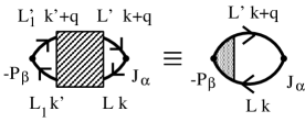
Figure 2: The Bethe–Salpeter expression for the screened dynamical conductivity tensor $\widetilde{\sigma}_{\alpha\beta}({\bf q},{\rm i}\nu_{n})$ in a general multiband case. The dynamical conductivity $\sigma_{\alpha\beta}({\bf q},{\rm i}\nu_{n})$, equation (5), is the RPA-irreducible part of $\widetilde{\sigma}_{\alpha\beta}({\bf q},{\rm i}\nu_{n})$. Kubo95

To complete the response theory, we must take into account the relaxation processes describing the way in which electrons are scattered by static disorder, by other electons or by different types of boson modes. Since our primarily interest is in the low-dimensional systems where the quasi-particle pole weight in the single-electron Green’s function is strongly reduced by boson-mediated electron-electron interactions, we must calculate $\sigma_{\alpha\beta}({\bf q},\tau)$ beyond the common weak coupling theory (corresponding to second-order perturbation theory for the single-electron self-energy function). This means that in order to work out $\sigma_{\alpha\beta}({\bf q},\tau)$ we must use the general Bethe–Salpeter expression for the screened conductivity tensor illustrated in figure 2 and the definition $\sum_{\beta}\sigma_{\alpha\beta}({\bf q},\omega)E_{\beta}({\bf q},\omega)=\sum_{\beta}\widetilde{\sigma}_{\alpha\beta}({\bf q},\omega)E_{0\beta}({\bf q},\omega)$, where ${\bf E}_{0}({\bf q},\omega)$ is the external electric field Kubo95 . The bold solid lines in these two diagrams are the single-electron Green’s functions which satisfy the Dyson equation (1). The intraband and interband contributions to $\sigma_{\alpha\beta}({\bf q},{\rm i}\nu_{n})=\sum_{LL^{\prime}}\sigma_{\alpha\beta}^{LL^{\prime}}({\bf q},{\rm i}\nu_{n})$ can be represented by the same expression,

$$\sigma_{\alpha\beta}^{LL^{\prime}}({\bf q},{\rm i}\nu_{n})=\frac{1}{V}\sum_{{\bf k}\sigma}\frac{1}{\beta\hbar^{2}}\sum_{{\rm i}\omega_{n}}J_{\alpha}^{LL^{\prime}}({\bf k}){\cal G}_{L}({\bf k},{\rm i}\omega_{n})$$

$$\hskip 14.22636pt\times{\cal G}_{L^{\prime}}({\bf k}_{+},{\rm i}\omega_{n+})(-)\Gamma^{LL^{\prime}}_{\beta}({\bf k},{\bf k}_{+},{\rm i}\omega_{n},{\rm i}\omega_{n+}),$$ (6)

equally well for $L=L^{\prime}$ as for $L\neq L^{\prime}$. Here the $\Gamma^{LL^{\prime}}_{\beta}({\bf k},{\bf k}_{+},{\rm i}\omega_{n},{\rm i}\omega_{n+})$ are the renormalized dipole vertex functions which satisfy the self-consistent Bethe–Salpeter equations for the renormalized dipole vertex, and ${\rm i}\omega_{n+}={\rm i}\omega_{n}+{\rm i}\nu_{n}$. In order to emphasize the connection between the present approach and the common transport theory, as well as to simplify the notation, we introduce the auxiliary electron-hole propagator $\Phi^{LL^{\prime}}_{\beta}({\bf k},{\bf k}_{+},{\rm i}\omega_{n},{\rm i}\omega_{n+})$ by comparing the relation

$$\sigma_{\alpha\beta}^{LL^{\prime}}({\bf q},{\rm i}\nu_{n})=\frac{1}{\beta V}\sum_{i\omega_{n}{\bf k}\sigma}J_{\alpha}^{LL^{\prime}}({\bf k})\Phi^{LL^{\prime}}_{\beta}({\bf k},{\bf k}_{+},{\rm i}\omega_{n},{\rm i}\omega_{n+})$$ (7)

with (6). Therefore, our task is to solve the self-consistent equations for $\Phi^{LL^{\prime}}_{\beta}({\bf k},{\bf k}_{+},{\rm i}\omega_{n},{\rm i}\omega_{n+})$ rather than that for the renormalized dipole vertices.

We limit our discussion to the low-dimensional systems where the scattering by static disorder and the scattering processes in which electrons change the band can both be neglected. These processes have negligible influence on the properties studied here. However, the self-consistent equations still have a very complex structure in particular as a consequence of the following features: the nesting properties of the Fermi surface, the resonant nature of the scattering by the (quasi)static CDW or SDW potentials and the local-field effects in the interband conductivity channel.

II.3 Results

The results of the present analysis are the following: (i) we show the formal solution to the Bethe–Salpeter equations for $\Phi^{LL^{\prime}}_{\alpha}({\bf k},{\bf k}_{+},{\rm i}\omega_{n},{\rm i}\omega_{n+})$ and to the (intraband) quantum transport equation, (ii) we compare the intraband conductivity to that obtained by using the memory-function approximation, (iii) we calculate the bare interband conductivity and (iv) we rederive the well-known Lorentz–Lorenz form of the optical conductivity in the presence of scattering by boson modes.

(i) Although it is tempting to completely neglect the electron-EM field vertex corrections in $\sigma_{\alpha\beta}({\bf q},{\rm i}\nu_{n})$, this is not justified in the intraband channel, at least in the cases with low-dimensional conductivity studied here. The method by which the intraband conductivity tensor is calculated here is very general and is based on a systematic analysis of the self-consistent equation for the auxiliary electron-hole propagator $\Phi_{\beta}({\bf k},{\bf k}_{+},{\rm i}\omega_{n},{\rm i}\omega_{n+})$ in which the single-electron self-energy contributions and the related vertex corrections are treated on an equal footing. The equation is of the form

$$\big{[}{\rm i}\nu_{n}+\varepsilon({\bf k})/\hbar-\varepsilon({\bf k}_{+})/\hbar$$

$$\hskip 28.45274pt+\Pi({\bf k},{\bf k}_{+},{\rm i}\omega_{n},{\rm i}\omega_{n+})\big{]}\Phi_{\alpha}({\bf k},{\bf k}_{+},{\rm i}\omega_{n},{\rm i}\omega_{n+})$$

$$\hskip 14.22636pt=\frac{1}{\hbar^{2}}\big{[}{\cal G}({\bf k},{\rm i}\omega_{n})-{\cal G}({\bf k}_{+},{\rm i}\omega_{n+})\big{]}p_{\alpha}(-{\bf q}),$$ (8)

with $p_{\alpha}(-{\bf q})={\rm i}e/q_{\alpha}$ and $\Pi({\bf k},{\bf k}_{+},{\rm i}\omega_{n},{\rm i}\omega_{n+})=\Pi^{r}({\bf k},{\bf k}_{+},{\rm i}\omega_{n},{\rm i}\omega_{n+})+{\rm i}\Pi^{i}({\bf k},{\bf k}_{+},{\rm i}\omega_{n},{\rm i}\omega_{n+})$. For simplicity we assume that only one band intersects the Fermi level and omit explicit reference to the conduction band index. $\Pi({\bf k},{\bf k}_{+},{\rm i}\omega_{n},{\rm i}\omega_{n+})$ is the electron-hole self-energy, the structure of which is derived here for the case in which conduction electrons are scattered only by various boson modes. These boson modes are assumed to dissipate momentum by their own means (impurities, Umklapps, etc.). Pinned phasons of the commensurate CDW problem, for example, enter in the present theory in the same way as the infrared-active optical phonons from section 8.2. This question is discussed in more details in Article II.

The electron-hole self-energy is found to be the difference between two auxiliary single-electron self-energies $\widetilde{\Sigma}({\bf k},{\rm i}\omega_{n})$, and the contributions of the ${\bf q}\approx 0$ forward scattering processes are found to drop out of both $\widetilde{\Sigma}({\bf k},{\rm i}\omega_{n})$ and $\Pi({\bf k},{\bf k}_{+},{\rm i}\omega_{n},{\rm i}\omega_{n+})$, in full agreement with the charge continuity equation.

Equation (8) is valid under quite general conditions, and is therefore applicable to a rich variety of problems, including purely electronic models with nonretarded local and short-range interactions. For example, it is not hard to verify that the normal scattering processes do not lead to the resistivity in this case, as required by the general principle of microscopic reversibility. Ziman72 This question will be discussed in more details in Ref. KupcicUP, .

(ii) In the ordinary 3D metallic regime, equation (8) leads to the ordinary transport equation, with Pines89 ; Ziman72

$$\sigma^{\rm intra}_{\alpha\alpha}({\bf q},\omega)\approx\frac{{\rm i}e^{2}}{m}\frac{1}{V}\sum_{{\bf k}\sigma}\frac{mv^{2}_{\alpha}({\bf k})\big{(}-\partial f({\bf k})/\partial E({\bf k})\big{)}}{\omega+{\rm i}\Gamma_{1\alpha}({\bf k})-q_{\alpha}^{2}v^{2}_{\alpha}({\bf k})/\omega}$$ (9)

being the resulting intraband electrical conductivity, and ${\bf q}=q_{\alpha}\hat{e}_{\alpha}$ again. Here, $m$ is the unity of mass, commonly taken as the free electron mass, and $\Gamma_{1\alpha}({\bf k})\propto\Pi^{i}({\bf k},{\bf k}_{+},{\rm i}\omega_{n},{\rm i}\omega_{n+})$ is the intraband relaxation rate. In the Drude $\omega\approx 0$ limit, where $\omega\gg q_{\alpha}v_{\alpha}({\bf k})$, the $q_{\alpha}$ dependent term in the denominator of (9) can be ignored, and we obtain the intraband conductivity (10). For $\omega\ll q_{\alpha}v_{\alpha}({\bf k})$ and $q_{\alpha}\rightarrow 0$, on the other hand, the result is the well-known Thomas–Fermi expression Ziman79 ; Mahan90 for $\sigma^{\rm intra}_{\alpha\alpha}({\bf q},\omega)$ and for the dielectric susceptibility $\chi^{\rm intra}({\bf q},\omega)=(q_{\alpha}^{2}/{\rm i}\omega)\sigma^{\rm intra}_{\alpha\alpha}({\bf q},\omega)$.

(iii) The general expression for the interband single-particle conductivity is derived and compared to the approximate expression which is frequently encountered in the literature. Wooten72 ; Ziman79

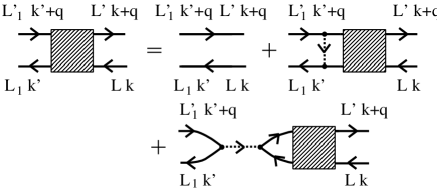
Figure 3: The Bethe–Salpeter equations for electron-hole propagators in a general multiband electronic model with weak nonretarded and/or boson-mediated electron-electron interactions. The vertex renormalizations are assumed to be negligible in this case.

(iv) If the scattering of valence electrons is sufficiently weak, the electron-boson vertex renormalizations are of no importance and the electron-hole propagators of figure 2 satisfy the Bethe–Salpeter equations shown in figure 3 with two types of contributions, the ladder contributions and the RPA (random phase approximation) contributions. Negele88 These equations can be completely rewritten in terms of the renormalized single-electron Green’s functions and the dynamically screened electron-electron interactions.

This approximation is used here to illustrate how the conductivity tensor is affected by the short-range dipole-dipole interactions. The result is the well-known Lorentz-Lorenz form of the dynamical conductivity for 3D metallic $sp_{\alpha}$ models Adler62 ; Wieser62 which is believed to be valid in the Q1D conductors, as well Zupanovic96 . From the result

$$\sigma^{\rm intra}_{\alpha\alpha}({\bf q},\omega)=\sigma^{\rm intra,0}_{\alpha\alpha}({\bf q},\omega)=\frac{{\rm i}e^{2}n_{\alpha\alpha}^{\rm eff}/m}{\omega+{\rm i}\Gamma_{1\alpha}},$$ (10)

$$\sigma^{\rm inter}_{\alpha\alpha}({\bf q},\omega)=\frac{\sigma^{\rm inter,0}_{\alpha\alpha}({\bf q},\omega)}{1-(4\pi{\rm i}/3\omega)\sigma^{\rm inter,0}_{\alpha\alpha}({\bf q},\omega)},$$ (11)

we can conclude that the contributions to the conductivity tensor of the free charges and of the bound charges are decoupled and that the Lorentz dipole-dipole interactions affect only the bound (interband) charge contribution to the conductivity tensor.

III Electron-boson coupling

Let us first introduce the quantities characterizing a general multiband electronic model with boson-mediated electron-electron interactions. The total Hamiltonian is the sum of two contributions, $H=H_{0}+H^{\prime}$. Here,

$$H_{0}=H_{0}^{\rm el}+H_{0}^{\rm bos}=\sum_{L{\bf k}\sigma}\varepsilon_{L}({\bf k})c^{\dagger}_{L{\bf k}\sigma}c_{L{\bf k}\sigma}$$

$$+\sum_{\nu{\bf q}^{\prime}}\frac{1}{2M_{\nu}}\big{[}p^{\dagger}_{\nu{\bf q}^{\prime}}p_{\nu{\bf q}^{\prime}}+\big{(}M_{\nu}\omega_{\nu{\bf q}^{\prime}}\big{)}^{2}q^{\dagger}_{\nu{\bf q}^{\prime}}q_{\nu{\bf q}^{\prime}}\big{]}$$ (12)

is the bare electron-boson Hamiltonian, and

$$H^{\prime}=\sum_{\nu{\bf q}^{\prime}}\sum_{LL^{\prime}{\bf k}\sigma}\Phi^{L^{\prime}L}_{\nu}({\bf k}+{\bf q}^{\prime},{\bf k})c^{\dagger}_{L^{\prime}{\bf k}+{\bf q}^{\prime}\sigma}c_{L{\bf k}\sigma}$$ (13)

is the scattering Hamiltonian which describes the scattering of valence electrons by each of the boson modes. As already mentioned, the bosonic modes can be external to electronic system (e.g. phonons) or built from electron-hole fluctuations at finite wave vectors. In (12), $\varepsilon_{L}({\bf k})$ is the bare electron dispersion, $\omega_{\nu{\bf q}^{\prime}}$ is the bare boson frequency and $M_{\nu}$ is the corresponding “mass” parameter. Finally, $\Phi^{L^{\prime}L}_{\nu}({\bf k}+{\bf q}^{\prime},{\bf k})$ is the generalized scattering potential. For convenience, it is assumed to be a product of the coupling constant $g_{\nu}/\sqrt{N}$, the dimensionless electron-boson vertex $q^{L^{\prime}L}_{\nu}({\bf k}+{\bf q}^{\prime},{\bf k})$ and the boson field $q_{\nu{\bf q}^{\prime}}$,

$$\Phi^{L^{\prime}L}_{\nu}({\bf k}+{\bf q}^{\prime},{\bf k})=\frac{g_{\nu}}{\sqrt{N}}\,q^{L^{\prime}L}_{\nu}({\bf k}+{\bf q}^{\prime},{\bf k})q_{\nu{\bf q}^{\prime}}.$$ (14)

In the intraband scattering approximation, in which the electron does not change the band when it is scattered by bosons, the scattering potential $\Phi^{L^{\prime}L}_{\nu}({\bf k}+{\bf q}^{\prime},{\bf k})$ is diagonal in the band index.

III.1 Skeleton diagrams

Figure 4: The Dyson equation (16) for boson Green’s functions.

In the finite temperature formalism, the effects of $H^{\prime}$ on the single-electron and boson properties are described in terms of two exact Matsubara Green’s functions Fetter71 ; Abrikosov75 ; Mahan90

$${\cal G}_{L}({\bf k},\tau)=-\langle T_{\tau}\big{[}c_{L{\bf k}\sigma}(\tau)c^{\dagger}_{L{\bf k}\sigma}(0)\big{]}\rangle,$$

$${\cal D}_{\nu}({\bf q}^{\prime},\tau)=-\langle T_{\tau}\big{[}q_{\nu{\bf q}^{\prime}}(\tau)q^{\dagger}_{\nu{\bf q}^{\prime}}(0)\big{]}\rangle.$$ (15)

Their Fourier transforms satisfy two Dyson equations, equation (1) and

$$\big{\{}M_{\nu}\big{[}({\rm i}\nu_{n})^{2}-\omega_{\nu{\bf q}^{\prime}}^{2}\big{]}-\hbar\Sigma_{\nu}({\bf q}^{\prime},{\rm i}\nu_{n})\big{\}}{\cal D}_{\nu}({\bf q}^{\prime},{\rm i}\nu_{n})=\hbar$$ (16)

(see figure 4). It is convenient to adopt an abbreviated notation by writting

$$\frac{g_{\nu}^{2}}{N}|q_{\nu}^{L^{\prime}L}({\bf k}+{\bf q}^{\prime},{\bf k})|^{2}{\cal D}_{\nu}({\bf q}^{\prime},\tau)\equiv\hbar{\cal F}_{\nu}^{L^{\prime}L}({\bf k}+{\bf q}^{\prime},{\bf k},\tau).$$ (17)

This expression can also be shown in the form ${\cal F}_{\nu}^{L^{\prime}L}({\bf k}+{\bf q}^{\prime},{\bf k},\tau)={\cal F}_{\nu}^{L^{\prime}L,LL^{\prime}}({\bf k}+{\bf q}^{\prime},{\bf k},{\bf q}^{\prime},\tau)$, where

$$\hbar{\cal F}_{\nu}^{L^{\prime}L,L_{1}L_{1}^{\prime}}({\bf k}+{\bf q}^{\prime},{\bf k}^{\prime},{\bf q}^{\prime},\tau)$$

$$=-\langle T_{\tau}\big{[}\Phi^{L^{\prime}L}_{\nu}({\bf k}+{\bf q}^{\prime},{\bf k},\tau)\Phi^{L_{1}L_{1}^{\prime}}_{\nu}({\bf k}^{\prime},{\bf k}^{\prime}+{\bf q}^{\prime},0)\big{]}\rangle,$$ (18)

is by definition the force-force correlation function Mahan90 ; Kupcic09 (FFCF) associated with the potential $\Phi^{L^{\prime}L}_{\nu}({\bf k}+{\bf q}^{\prime},{\bf k})$.

Figure 5: The skeleton series for the single-electron self-energy. The self-energy is shown in terms of both the renormalized three-point vertex function $\tilde{q}_{\nu}^{L^{\prime}L}({\bf k}_{+},{\bf k},{\rm i}\omega_{n+},{\rm i}\omega_{n})$ (the big gray circle) and the completely irreducible four-point vertex function $U_{\nu}^{L^{\prime}L,LL^{\prime}}({\bf k}+{\bf q}^{\prime},{\bf k},{\bf q}^{\prime},{\rm i}\omega_{n+},{\rm i}\omega_{n},{\rm i}\nu_{n})$ (the white rectangle).

In high-order perturbation theory the self-energy function of the electron, $\Sigma_{L}({\bf k},{\rm i}\omega_{n})$, is usually represented by the sum of skeleton diagrams shown in figure 5, leading to a simple analytical expression

$$\hbar\Sigma_{L}({\bf k},{\rm i}\omega_{n})\approx-\sum_{L^{\prime}\nu{\bf q}^{\prime}}\frac{1}{\beta\hbar}\sum_{{\rm i}\nu_{n}}{\cal G}_{L^{\prime}}({\bf k}+{\bf q}^{\prime},{\rm i}\omega_{n+})$$

$$\hskip 14.22636pt\times\widetilde{\cal F}_{\nu}^{L^{\prime}L,LL^{\prime}}({\bf k}+{\bf q}^{\prime},{\bf k},{\bf q}^{\prime},{\rm i}\omega_{n+},{\rm i}\omega_{n}).$$ (19)

Here, $\widetilde{\cal F}_{\nu}^{L^{\prime}L,LL^{\prime}}({\bf k}+{\bf q}^{\prime},{\bf k},{\bf q}^{\prime},{\rm i}\omega_{n+},{\rm i}\omega_{n})$ is the renormalized FFCF obtained by replacing one bare electron-boson vertex in ${\cal F}_{\nu}^{L^{\prime}L,LL^{\prime}}({\bf k}+{\bf q}^{\prime},{\bf k},{\bf q}^{\prime},{\rm i}\nu_{n})$, $q_{\nu}^{L^{\prime}L}({\bf k}_{+},{\bf k})$, by the renormalized vertex $\tilde{q}_{\nu}^{L^{\prime}L}({\bf k}_{+},{\bf k},{\rm i}\omega_{n+},{\rm i}\omega_{n})$. Equation (19) is nothing but the three-point vertex representation of $\Sigma_{L}({\bf k},{\rm i}\omega_{n})$. In the same representation the boson self-energy takes the form

$$\hbar\Sigma_{\nu}({\bf q},{\rm i}\nu_{n})\approx\sum_{LL^{\prime}{\bf k}\sigma}\frac{1}{\beta\hbar^{2}}\sum_{{\rm i}\omega_{n}}\frac{g_{\nu}^{2}}{N}\tilde{q}_{\nu}^{L^{\prime}L}({\bf k}_{+},{\bf k},{\rm i}\omega_{n+},{\rm i}\omega_{n})$$

$$\hskip 28.45274pt\times q_{\nu}^{LL^{\prime}}({\bf k},{\bf k}_{+}){\cal G}_{L}({\bf k},{\rm i}\omega_{n}){\cal G}_{L^{\prime}}({\bf k}_{+},{\rm i}\omega_{n+}).$$ (20)

We have just reemphasized that the three-point vertex representation is very useful in describing the closed system of four equations characterizing strongly-interacting electron-boson systems in the absence of external EM fields (equations (1), (16), (19) and (20)). However, the conductivity tensor of such an electron-boson model has a compact form if the structure of the Bethe–Salpeter equations of section 6 is also simple, at least from the formal point of view. For this purpose, it is much more convenient to use the four-point vertex representation. This representation is based upon the knowledge of the irreducible four-point interaction $U_{\nu}^{L^{\prime}L,LL^{\prime}}({\bf k}+{\bf q}^{\prime},{\bf k},{\bf q}^{\prime},{\rm i}\omega_{n+},{\rm i}\omega_{n},{\rm i}\nu_{n})$. The equivalence of the two representations in the skeleton approximation is illustrated in figure 5, where $U_{\nu}^{L^{\prime}L,LL^{\prime}}({\bf k}+{\bf q}^{\prime},{\bf k},{\bf q}^{\prime},{\rm i}\omega_{n+},{\rm i}\omega_{n},{\rm i}\nu_{n})$ is represented by the white rectangle. The expression for $\Sigma_{L}({\bf k},{\rm i}\omega_{n})$ is now of the form

$$\hbar\Sigma_{L}({\bf k},{\rm i}\omega_{n})\approx-\sum_{L^{\prime}\nu{\bf q}^{\prime}}\frac{1}{\beta\hbar}\sum_{{\rm i}\nu_{n}}{\cal G}_{L^{\prime}}({\bf k}+{\bf q}^{\prime},{\rm i}\omega_{n+})$$

$$\times U_{\nu}^{L^{\prime}L,LL^{\prime}}({\bf k}+{\bf q}^{\prime},{\bf k},{\bf q}^{\prime},{\rm i}\omega_{n+},{\rm i}\omega_{n},{\rm i}\nu_{n}).$$ (21)

A full discussion of the Bethe–Salpeter equations is postponed to section 6.

IV Electron coupling to EM fields

In quantum electrodynamics of tightly bound valence electrons in solids, whether metallic or insulating, the coupling between electrons and external EM fields is given by the minimal gauge invariant substitution. The expansion to the second order in the vector potential $A_{\alpha}({\bf q},\omega)$ gives the coupling Hamiltonian $H^{\rm ext}\approx\widetilde{H}^{\rm ext}_{1}+\widetilde{H}^{\rm ext}_{2}$, with Kupcic07 ; Kupcic04 ; Kupcic05

$$\widetilde{H}^{\rm ext}_{1}=-\frac{1}{c}\sum_{{\bf q}\alpha}A_{\alpha}({\bf q})\hat{J}_{\alpha}(-{\bf q}),$$

$$\widetilde{H}^{\rm ext}_{2}=\frac{e^{2}}{2mc^{2}}\sum_{{\bf q}{\bf q}^{\prime}\alpha\beta}A_{\alpha}({\bf q}-{\bf q}^{\prime})A_{\beta}({\bf q}^{\prime})\hat{\gamma}^{LL}_{\alpha\beta}(-{\bf q};2).$$ (22)

Here,

$$\hat{J}_{\alpha}({\bf q})=\sum_{LL^{\prime}}\sum_{{\bf k}\sigma}J_{\alpha}^{LL^{\prime}}({\bf k},{\bf k}_{+})c^{\dagger}_{L{\bf k}\sigma}c_{L^{\prime}{\bf k}+{\bf q}\sigma},$$

$$\hat{\gamma}^{LL}_{\alpha\beta}({\bf q};2)=\sum_{L}\sum_{{\bf k}\sigma}\gamma^{LL}_{\alpha\beta}({\bf k},{\bf k}_{+};2)c^{\dagger}_{L{\bf k}\sigma}c_{L{\bf k}+{\bf q}\sigma}$$ (23)

are, respectively, the total current density operator and the bare diamagnetic density operator.

To obtain the semiclassical expression for the coupling Hamiltonian, equation (2), we have to take into account the fact that both the interband and intraband current-current contributions to the diamagnetic current must vanish in the normal metallic or insulating state. The cancellation of the interband contribution is a consequence of the effective mass theorem, Abrikosov73 ; Kupcic07 ; Kupcic04 ; Kupcic03

$$\gamma^{LL}_{\alpha\beta}({\bf k})=\gamma^{LL}_{\alpha\beta}({\bf k};2)+\sum_{L^{\prime}(\neq L)}\frac{(2m/e^{2})J_{\alpha}^{LL^{\prime}}({\bf k})J_{\beta}^{L^{\prime}L}({\bf k})}{\varepsilon_{L}({\bf k})-\varepsilon_{L^{\prime}}({\bf k})}$$

$$\hskip 5.69054pt=\frac{m}{\hbar^{2}}\frac{\partial^{2}\varepsilon_{L}({\bf k})}{\partial k_{\alpha}\partial k_{\beta}},$$ (24)

leading to $H^{\rm ext}\approx H^{\rm ext}_{1}+H^{\rm ext}_{2}$, with Kupcic09

$$H^{\rm ext}_{1}=-\frac{1}{c}\sum_{{\bf q}\alpha}A_{\alpha}({\bf q})\bigg{[}{\sum_{L}}\hat{J}^{LL}_{\alpha}(-{\bf q})+\sum_{L\neq L^{\prime}}{\rm i}\omega\hat{P}^{LL^{\prime}}_{\alpha}(-{\bf q})\bigg{]},$$

$$H^{\rm ext}_{2}=\frac{e^{2}}{2mc^{2}}\sum_{L{\bf q}{\bf q}^{\prime}\alpha\beta}A_{\alpha}({\bf q}-{\bf q}^{\prime})A_{\beta}({\bf q}^{\prime})\hat{\gamma}^{LL}_{\alpha\beta}(-{\bf q}).$$ (25)

Here, $\hat{P}_{\alpha}^{LL^{\prime}}({\bf q})$, $L\neq L^{\prime}$, is the interband part in dipole density operator (3), and $\hat{\gamma}^{LL}_{\alpha\beta}(-{\bf q})$ is the diamagnetic density operator. The reciprocal effective mass tensor $\gamma^{LL}_{\alpha\beta}({\bf k})$ is the vertex function in $\hat{\gamma}^{LL}_{\alpha\beta}(-{\bf q})$.

The intraband current-current contribution to the diamagnetic current cancels $H^{\rm ext}_{2}$, confirming the assertion made in section 2 that

$$H^{\rm ext}=-\sum_{{\bf q}\alpha}E_{\alpha}({\bf q})\hat{P}_{\alpha}({-\bf q}).$$

We emphasize the simple structure of this coupling Hamiltonian. The most direct way to obtain this expression for $H^{\rm ext}$ is to consider the coupling of the scalar potential $V^{\rm tot}({\bf q},\omega)$ to the charge density operator. Kubo95

IV.1 Density operators

Let us derive now the relations (4) among three types of intraband and interband vertex functions underlying the gauge invariance of the present response theory. To do this, we use very general microscopic operator equations

$$\hbar q_{\alpha}\hat{J}_{\alpha}({\bf q})={\rm i}\hbar\frac{\partial}{\partial t}\hat{\rho}({\bf q})=\big{[}\hat{\rho}({\bf q}),H_{0}^{\rm el}\big{]},$$

$${\rm i}\hbar\hat{J}_{\alpha}({\bf q})={\rm i}\hbar\frac{\partial}{\partial t}\hat{P}_{\alpha}({\bf q})=\big{[}\hat{P}_{\alpha}({\bf q}),H_{0}^{\rm el}\big{]},$$ (26)

where $H_{0}^{\rm el}$ is the electronic part in the bare Hamiltonian (12). Furthermore,

$$\hat{\rho}({\bf q})=\sum_{LL^{\prime}}\sum_{{\bf k}\sigma}eq^{LL^{\prime}}({\bf k},{\bf k}_{+})c^{\dagger}_{L{\bf k}\sigma}c_{L^{\prime}{\bf k}+{\bf q}\sigma}$$ (27)

is the total charge density operator, with $eq^{LL^{\prime}}({\bf k},{\bf k}_{+})$ being the charge vertex function, while $\hat{J}_{\alpha}({\bf q})$ and $\hat{P}_{\alpha}({\bf q})$ are given by (23) and (3). The two commutators in (26) are easily worked out, leading to the required relations

$$P_{\alpha}^{LL^{\prime}}({\bf k},{\bf k}_{+})=\frac{{\rm i}\hbar J_{\alpha}^{LL^{\prime}}({\bf k})}{\varepsilon_{L^{\prime}}({\bf k}_{+})-\varepsilon_{L}({\bf k})}=\frac{{\rm i}e}{q_{\alpha}}\,q^{LL^{\prime}}({\bf k},{\bf k}_{+}).$$

The explicit form of each of these vertices is often obtained by calculating the coefficients in the linear term in $H^{\rm ext}$ in (22).

The long-wavelength intraband vertices are of particular interest. They are given by model independent expressions

$$q^{LL}({\bf k},{\bf k}_{+})\approx 1,$$

$$J^{LL}_{\alpha}({\bf k},{\bf k}_{+})\approx J^{LL}_{\alpha}({\bf k})\equiv ev^{L,0}_{\alpha}({\bf k}),$$

$$P^{LL}_{\alpha}({\bf k},{\bf k}_{+})\approx P^{LL}_{\alpha}(-{\bf q})\equiv p_{\alpha}(-{\bf q}).$$ (28)

Here, $v^{L,0}_{\alpha}({\bf k})=(1/\hbar)\partial\varepsilon_{L}({\bf k})/\partial k_{\alpha}$ is the bare electron group velocity and $p_{\alpha}(-{\bf q})={\rm i}e/q_{\alpha}$ is the bare dipole vertex.

Notice that the thermodynamic averages of the density operators in (26) are the usual induced macroscopic densities. For example, ${\bf J}({\bf q},\omega)$, $\rho({\bf q},\omega)$ and ${\bf P}({\bf q},\omega)$ represent the common notation for the induced macroscopic current, charge and dipole densities. They are related by two equations Landau95

$${\bf q}\cdot{\bf J}({\bf q},\omega)=\omega\rho({\bf q},\omega),$$

$$\rho({\bf q},\omega)=-{\rm i}{\bf q}\cdot{\bf P}({\bf q},\omega).$$ (29)

The first one is the usual charge continuity equation.

V Dynamical conductivity tensor

We now define the total dynamical conductivity tensor $\sigma_{\alpha\beta}({\bf q},\omega)$ as the response function to the macroscopic electric field Landau95

$${\bf E}({\bf q},\omega)={\bf E}_{0}({\bf q},\omega)+{\bf E}_{1}({\bf q},\omega);$$ (30)

that is

$$J_{\alpha}({\bf q},\omega)=\sum_{\beta}\sigma_{\alpha\beta}({\bf q},\omega)E_{\beta}({\bf q},\omega).$$ (31)

Here, ${\bf J}({\bf q},\omega)$ is the induced total current density from (29), ${\bf E}_{0}({\bf q},\omega)$ is the external field and ${\bf E}_{1}({\bf q},\omega)$ is the depolarization field (equal to $-4\pi{\bf P}({\bf q},\omega)$ for the longitudinal polarization of the field in the thin slab). The conductivity tensor is given by analytical continuation to the real axis of $\sigma_{\alpha\beta}({\bf q},{\rm i}\nu_{n})$ (see figure 6), where $\sigma_{\alpha\beta}({\bf q},{\rm i}\nu_{n})$ is the Matsubara Fourier transform of

$$\sigma_{\alpha\beta}({\bf q},\tau)=\frac{1}{\hbar V}\langle T_{\tau}[\hat{J}_{\alpha}({\bf q},\tau)\hat{P}_{\beta}(-{\bf q},0)]\rangle_{\rm irred}.$$

Therefore, to find the dynamical conductivity tensor of an interacting electron-boson system, we must determine the structure of the current-dipole Kubo formula (5) which agrees with the definition of the macroscopic electric field (30).

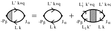
Figure 6: The dynamical conductivity $\sigma_{\alpha\beta}({\bf q},{\rm i}\nu_{n})$ from figure 2, shown in the three-point vertex representation (left diagram) and in the four-point vertex representation (right diagrams). The collection of diagrams in the renormalized four-point interaction must be consistent with the definition of ${\bf E}({\bf q},\omega)$ in (30); i.e., the renormalized four-point interaction is irreducible in the long-range RPA contribution.

V.1 Relaxation-time approximation

It is instructive first to show the structure of the bare dynamical conductivity (5) in the simplest multiband model, namely, a two-band model with the lower band partially occupied by electrons and the upper band empty, in the limiting case where the scattering is sufficiently weak. As explained in more details in Article II, this model is of importance in accounting for the properties of the ordered state of some simple CDW systems. Lee74 ; Kim93 ; Kupcic09

To do this, we first calculate the ideal bare conductivity tensor $\sigma^{0}_{\alpha\beta}({\bf q},{\rm i}\nu_{n})$ which is given by the first term in figure 6, with ${\cal G}_{L}({\bf q},{\rm i}\omega_{n})$ replaced by the bare Green’s function ${\cal G}_{L}^{0}({\bf q},{\rm i}\omega_{n})$. Summation over ${\rm i}\omega_{n}$ can be performed easily to give $\sigma^{0}_{\alpha\beta}({\bf q},{\rm i}\nu_{n})=\delta_{\alpha,\beta}\sum_{LL^{\prime}}\sigma_{\alpha\alpha}^{LL^{\prime}}({\bf q},{\rm i}\nu_{n})$. After analytical continuation, we obtain the ideal bare intraband ($L=L^{\prime}$) and interband ($L\neq L^{\prime}$) contributions described by

$$\sigma_{\alpha\alpha}^{LL^{\prime}}({\bf q},\omega)$$

$$=-\frac{1}{V}\sum_{{\bf k}\sigma}\frac{J_{\alpha}^{LL^{\prime}}({\bf k})P_{\alpha}^{L^{\prime}L}({\bf k})[f_{L}({\bf k})-f_{L^{\prime}}({\bf k}_{+})]}{\hbar\omega+{\rm i}\hbar\eta+\varepsilon_{L}({\bf k})-\varepsilon_{L^{\prime}}({\bf k}_{+})}.$$ (32)

Weak scattering processes can be inserted into this expression by replacing the adiabatic term $\eta$ by the relaxation rate $\Gamma^{LL^{\prime}}_{\alpha}$ independent of frequency and wave vector. This is the generalization of the common relaxation-time approximation. As required, the associated transport relaxation time $\tau^{L}_{\alpha}=1/\Gamma^{LL}_{\alpha}$ differs from that found in the single-electron propagators.

The bare intraband contribution is of the Drude form

$$\sigma^{\rm intra,0}_{\alpha\alpha}({\bf q},\omega)\approx\frac{{\rm i}e^{2}n^{\rm eff,0}_{\alpha\alpha}/m}{\omega+{\rm i}\Gamma_{1\alpha}},$$ (33)

with

$$n_{\alpha\alpha}^{\rm eff,0}=\frac{1}{V}\sum_{L{\bf k}\sigma}m[v^{L,0}_{\alpha}({\bf k})]^{2}\bigg{(}-\frac{\partial f_{L}({\bf k})}{\partial\varepsilon_{L}({\bf k})}\bigg{)}$$ (34)

representing the effective number of conduction electrons, Kupcic07 ; Kupcic09 and $\Gamma^{LL}_{\alpha}=\Gamma_{1\alpha}$ by assumption. $n_{\alpha\alpha}^{\rm eff,0}$ includes the conduction holes from the lower band and the thermally activated electrons from the upper band. The bare interband contribution is the sum of two off-diagonal terms in (32), with $\eta$ replaced by $\Gamma^{LL^{\prime}}_{\alpha}$: $\sigma^{\rm inter,0}_{\alpha\alpha}({\bf q},\omega)=\sum_{L\neq L^{\prime}}\sigma^{LL^{\prime}}_{\alpha\alpha}({\bf q},\omega)$.

The main disadvantage of this simple procedure of calculating $\sigma_{\alpha\alpha}({\bf q},\omega)$ is that it does not apply to low-dimensional systems with sizeable interactions. The reason for that is the following. First, comparison with experimental data shows that the relaxation rates $\Gamma^{LL^{\prime}}_{\alpha}$ are frequency dependent. Second, the causality principle requires that $\Gamma^{LL^{\prime}}_{\alpha}(\omega)$ is just the imaginary part of a complex quantity which will be called here the electron-hole self-energy function. Finally, it turns out that in the strong coupling limit the electron-hole self-energy is not a simple function of frequency $\omega$. Instead, it depends quite drastically on two internal electron frequencies too.

We shall therefore present now a systematic treatment of scattering processes in interacting electron-boson systems with multiple electronic bands which treats all elements in the electron-hole self-energy consistently with the charge continuity equation (29), with the causality principle and with the definition of ${\bf E}({\bf q},\omega)$. The resulting self-consistent equations turn out to be the generalization of the equations used by Vollhardt and Wölfle Vollhardt80 to study the scattering by static disorder in a single-band case.

VI Bethe–Salpeter equations

Figure 7: The general form of the Bethe–Salpeter equations for electron-hole propagators. The white rectangle represents again the completely irreducible four-point interaction.

The term Bethe–Salpeter equations Negele88 ; Ziman88 refers to the self-consistent equations for the exact electron-hole propagators $\Phi^{LL^{\prime}L^{\prime}_{1}L_{1}}({\bf k},{\bf k}_{+},{\bf k}^{\prime}_{+},{\bf k}^{\prime},{\rm i}\omega_{n},{\rm i}\omega_{n+},{\rm i}\omega_{m+},{\rm i}\omega_{m})$ shown in figure 7. A widely-used simplification in these equations is illustrated in figure 3. In this case, we have both the ladder contributions and the RPA-like contributions to the irreducible four-point interaction, but the three-point vertex renormalizations are neglected both in these equations and in the related Dyson equations. The interaction lines and the electron propagators are renormalized, so that these equations must be treated consistently with the Dyson equations, as already pointed out in section 2. However, in strictly 1D metallic systems as well as in strongly-correlated low-dimensional systems, it is necessary to use the Bethe–Salpeter equations beyond this approximation by taking into account the three-point vertex renormalizations as well.

To simplify the analysis, it is convenient to multiply the left-hand side of the diagrams in figure 7 by the corresponding bare vertex function and then sum over ${\bf k}^{\prime}$ and ${\rm i}\omega_{m}$. For the electron-hole propagators in the dynamical conductivity (5), the bare vertex in question is the bare dipole vertex function, and the Bethe–Salpeter equations from figure 7 turn into the Bethe–Salpeter equations for the auxiliary electron-hole propagators

$$\Phi^{LL^{\prime}}_{\alpha}({\bf k},{\bf k}_{+},{\rm i}\omega_{n},{\rm i}\omega_{n+})=\frac{1}{\hbar^{2}}{\cal G}_{L}({\bf k},{\rm i}\omega_{n})$$

$$\times{\cal G}_{L^{\prime}}({\bf k}_{+},{\rm i}\omega_{n+})(-)\Gamma^{LL^{\prime}}_{\alpha}({\bf k},{\bf k}_{+},{\rm i}\omega_{n},{\rm i}\omega_{n+}).$$ (35)

The equations are illustrated in figure 8.

With little loss of generality, we restrict the analysis to the case where the irreducible four-point interaction $\sum_{\nu}U_{\nu}^{L^{\prime}L_{1}^{\prime},L_{1}L}({\bf k}_{+},{\bf k}^{\prime},{\bf q}^{\prime},{\rm i}\omega_{n+},{\rm i}\omega_{m},{\rm i}\nu_{m})$ can be approximated by $U^{L^{\prime}L_{1}^{\prime},L_{1}L}({\bf q}^{\prime},{\rm i}\nu_{m})$. In this case, the explicit form of the intraband ($L=L^{\prime}$) and interband ($L\neq L^{\prime}$) equations is the following

$$D_{LL^{\prime}}^{-1}({\bf k},{\bf k}_{+},{\rm i}\omega_{n},{\rm i}\omega_{n+})\Phi^{LL^{\prime}}_{\alpha}({\bf k},{\bf k}_{+},{\rm i}\omega_{n},{\rm i}\omega_{n+})$$

$$\hskip 28.45274pt=\frac{1}{\hbar^{2}}\big{[}{\cal G}_{L}({\bf k},{\rm i}\omega_{n})-{\cal G}_{L^{\prime}}({\bf k}_{+},{\rm i}\omega_{n+})\big{]}$$

$$\times\bigg{\{}-P_{\alpha}^{L^{\prime}L}({\bf k}_{+},{\bf k})-\frac{1}{\beta}\sum_{L_{1}L_{1}^{\prime}}\sum_{{\bf q}^{\prime}{\rm i}\nu_{m}}U^{L^{\prime}L_{1}^{\prime},L_{1}L}({\bf q}^{\prime},{\rm i}\nu_{m})$$

$$\hskip 28.45274pt\times\Phi^{L_{1}L_{1}^{\prime}}_{\alpha}({\bf k}+{\bf q}^{\prime},{\bf k}_{+}+{\bf q}^{\prime},{\rm i}\omega_{m},{\rm i}\omega_{m+})\bigg{\}},$$ (36)

with

$$D_{LL^{\prime}}^{-1}({\bf k},{\bf k}_{+},{\rm i}\omega_{n},{\rm i}\omega_{n+})={\rm i}\nu_{n}+\varepsilon_{L}({\bf k})/\hbar-\varepsilon_{L^{\prime}}({\bf k}_{+})/\hbar$$

$$\hskip 56.9055pt+\Sigma_{L}({\bf k},{\rm i}\omega_{n})-\Sigma_{L^{\prime}}({\bf k}_{+},{\rm i}\omega_{n+})$$ (37)

and ${\rm i}\omega_{m}={\rm i}\omega_{n}+{\rm i}\nu_{m}$. The ${\cal G}_{L}({\bf k},{\rm i}\omega_{n})$ satisfy the Dyson equations for electrons (1) and $U^{L^{\prime}L_{1}^{\prime},L_{1}L}({\bf q}^{\prime},{\rm i}\nu_{m})$ is a simple generalization of the completely irreducible four-point interaction $U^{L^{\prime}L,LL^{\prime}}({\bf q}^{\prime},{\rm i}\nu_{m})$ from (21).

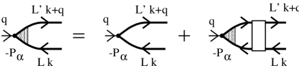
Figure 8: The Bethe-Salpeter equations (36) for auxiliary electron-hole propagators.

In the electronic multiband model we are interested in here, there are $n$ bands in the vicinity of the Fermi level. The bands are built of $n$ orbitals per unit cell. Associated with each of these orbitals are the intracell charge and spin fluctuations, and these intracell fluctuations are possible sources of scattering. The monopole charge fluctuations underlying the present analysis of the dynamical conductivity tensor might be also strongly affected by the presence of the intracell fluctuations. As a result, $\sigma_{\alpha\beta}({\bf q},\omega)$ will have considerably more structure than that characterizing the ordinary single-band model, even in the case where only one band out of $n$ valence bands intersects the Fermi level.

VI.1 Quantum transport equation

In the remainder of this section we consider the intraband term in (36) from this point of view. We assume that there is only one conduction band and again drop reference to the band index. We use the intraband scattering approximation where the scattering processes in which the electron changes the band are neglected. As discussed in Article II, this approximation is easily seen not to be adequate, for example, to study fluctuations in the order parameter in the pseudogap state of the ordinary CDW systems. However, it is convenient to illustrate the main ideas regarding the quantum transport equations. Finally, the three-point vertex renormalizations in the renormalized interactions are also neglected, as usual in the common non-crossing approximation for the electron-boson systems. Millis87 ; Niksic95 ; Rozenberg96 The resulting intraband Bethe–Salpeter equation is of the form

$$D^{-1}({\bf k},{\bf k}_{+},{\rm i}\omega_{n},{\rm i}\omega_{n+})\Phi_{\alpha}({\bf k},{\bf k}_{+},{\rm i}\omega_{n},{\rm i}\omega_{n+})$$

$$\hskip 14.22636pt=\frac{1}{\hbar^{2}}\big{[}{\cal G}({\bf k},{\rm i}\omega_{n})-{\cal G}({\bf k}_{+},{\rm i}\omega_{n+})\big{]}\bigg{\{}p_{\alpha}(-{\bf q})$$

$$-\frac{1}{\beta}\sum_{{\bf q}^{\prime}{\rm i}\nu_{m}}{\cal F}({\bf q}^{\prime},{\rm i}\nu_{m})\Phi_{\alpha}({\bf k}+{\bf q}^{\prime},{\bf k}_{+}+{\bf q}^{\prime},{\rm i}\omega_{m},{\rm i}\omega_{m+})\bigg{\}}.$$

(38)

The structure of (38) is simplified by defining the auxiliary single-electron self-energy function

$$\hbar\widetilde{\Sigma}({\bf k},{\rm i}\omega_{n})=-\frac{1}{\beta\hbar}\sum_{{\bf q}^{\prime}{\rm i}\nu_{m}}\bigg{\{}1-\frac{v^{0}_{\alpha}({\bf k}+{\bf q}^{\prime})}{v^{0}_{\alpha}({\bf k})}\bigg{\}}$$

$$\hskip 28.45274pt\times{\cal F}({\bf q}^{\prime},{\rm i}\nu_{m}){\cal G}({\bf k}+{\bf q}^{\prime},{\rm i}\omega_{n}+{\rm i}\nu_{m})$$ (39)

and the electron-hole self-energy

$$\Pi({\bf k},{\bf k}_{+},{\rm i}\omega_{n},{\rm i}\omega_{n+})=\widetilde{\Sigma}({\bf k},{\rm i}\omega_{n})-\widetilde{\Sigma}({\bf k}_{+},{\rm i}\omega_{n+}).$$ (40)

Equation (38) now reduces to the quantum transport equation

$$\big{[}{\rm i}\nu_{n}+\varepsilon({\bf k})/\hbar-\varepsilon({\bf k}_{+})/\hbar$$

$$+\Pi^{r}({\bf k},{\bf k}_{+},{\rm i}\omega_{n},{\rm i}\omega_{n+})\big{]}\Phi_{\alpha}({\bf k},{\bf k}_{+},{\rm i}\omega_{n},{\rm i}\omega_{n+})$$

$$\hskip 14.22636pt-\frac{1}{\hbar^{2}}\big{[}{\cal G}({\bf k},{\rm i}\omega_{n})-{\cal G}({\bf k}_{+},{\rm i}\omega_{n+})\big{]}p_{\alpha}(-{\bf q})$$

$$=-{\rm i}\Pi^{i}({\bf k},{\bf k}_{+},{\rm i}\omega_{n},{\rm i}\omega_{n+})\Phi_{\alpha}({\bf k},{\bf k}_{+},{\rm i}\omega_{n},{\rm i}\omega_{n+}).$$ (41)

Equation (41) is the self-consistent equation for the auxiliary electron-hole propagator, in contrast to the ordinary transport equation, equation (47), which is formulated in terms of the induced density $\delta n({\bf k},{\bf q},{\rm i}\nu_{n})$ defined by

$$\delta n({\bf k},{\bf q},{\rm i}\nu_{n})=\frac{1}{\beta}\sum_{{\rm i}\omega_{n}}\Phi_{\alpha}({\bf k},{\bf k}_{+},{\rm i}\omega_{n},{\rm i}\omega_{n+})E_{\alpha}({\bf q},{\rm i}\nu_{n}).$$ (42)

The conditions under which (41) reduces to the ordinary transport equation are discussed below.

To illustrate the role of the electron-EM field vertex renomalizations in (41), it is useful to define the auxiliary single-electron propagator $\widetilde{\cal G}({\bf k},{\rm i}\omega_{n})$ as the single-particle propagator which satisfies the following Dyson equation

$$\big{[}{\rm i}\hbar\omega_{n}-\varepsilon({\bf k})+\mu-\hbar\widetilde{\Sigma}({\bf k},{\rm i}\omega_{n})\big{]}\widetilde{\cal G}({\bf k},{\rm i}\omega_{n})=\hbar.$$ (43)

The forward scattering processes cancel identically out in $\widetilde{\Sigma}({\bf k},{\rm i}\omega_{n})$ as a result of the charge continuity equation. The fact that the auxiliary propagator $\widetilde{\cal G}({\bf k},{\rm i}\omega_{n})$ has the quasi-particle pole even for relatively strong scattering processes is consistent with the fact that the residue associated with the quasi-particle pole in the exact propagator ${\cal G}({\bf k},{\rm i}\omega_{n})$ is proportional to $t_{b}/t_{a}$ and vanishes in the strictly 1D limit $t_{b}\rightarrow 0$. Dzyaloshinskii73 This interesting observation is in the background of a variety of approximate treatments of various pseudogapped states. In these approaches, the forward scattering contributions to the FFCF ${\cal F}({\bf q}^{\prime},{\rm i}\nu_{m})$ are neglected from the outset.

The expression for the intraband conductivity which correctly describes the $\omega\approx 0$ Drude limit, but which is not necessarily correct in the $\omega=0$ Thomas–Fermi limit, is the following

$$\sigma_{\alpha\alpha}^{\rm intra}({\bf q},{\rm i}\nu_{n})=\frac{1}{V}\sum_{{\bf k}\sigma}J_{\alpha}({\bf k})p_{\alpha}(-{\bf q})\frac{1}{\beta\hbar}\sum_{{\rm i}\omega_{n}}$$

$$\times\frac{{\cal G}({\bf k},{\rm i}\omega_{n})-{\cal G}({\bf k}_{+},{\rm i}\omega_{n+})}{{\rm i}\hbar\nu_{n}+\hbar\Pi({\bf k},{\bf k}_{+},{\rm i}\omega_{n},{\rm i}\omega_{n+})+\varepsilon({\bf k})-\varepsilon({\bf k}_{+})}.$$ (44)

This is nothing but (32) for the ideal intraband conductivity in which ${\rm i}\eta$ is replaced by $\Pi({\bf k},{\bf k}_{+},{\rm i}\omega_{n},{\rm i}\omega_{n+})$.

VI.2 Memory-function approximation

In the weak coupling limit, the self-energy $\Pi({\bf k},{\bf k}_{+},{\rm i}\omega_{n},{\rm i}\omega_{n+})$ is a non-singular function of two fermion frequencies and in the simplest approximation can be written in the form $\Pi({\bf k},{\bf k}_{+},{\rm i}\omega_{n},{\rm i}\omega_{n+})\approx M_{\alpha}({\bf k},{\rm i}\nu_{n})=M^{r}_{\alpha}({\bf k},{\rm i}\nu_{n})+{\rm i}M^{i}_{\alpha}({\bf k},{\rm i}\nu_{n})$. $M_{\alpha}({\bf k},{\rm i}\nu_{n})$ is called the memory function. Gotze72 ; Giamarchi91 ; Kupcic04 The momentum distribution function

$$n({\bf k})=\frac{1}{\beta\hbar}\sum_{{\rm i}\omega_{n}}{\cal G}({\bf k},{\rm i}\omega_{n}){\rm e}^{{\rm i}\omega_{n}\eta}$$ (45)

appearing in (44) in the memory-function approximation reduces in the weak coupling limit to the Fermi–Dirac distribution function $f({\bf k})$.

We now define the electron-boson coupling function $\lambda_{\alpha}({\bf k},\omega)$, the mass enhancement factor $m_{\alpha\alpha}^{*}({\bf k},\omega)/m$, the intraband relaxation rate $\Gamma_{1\alpha}({\bf k},\omega)$ and the collision integral $I({\bf k},\omega)$ by

$$\lambda_{\alpha}({\bf k},\omega)=M^{r}_{\alpha}({\bf k},\omega)/\omega,$$

$$m_{\alpha\alpha}^{*}({\bf k},\omega)=(1+\lambda_{\alpha}({\bf k},\omega))m,$$

$$\Gamma_{1\alpha}({\bf k},\omega)=(m/m_{\alpha\alpha}^{*}({\bf k},\omega))M^{i}_{\alpha}({\bf k},\omega),$$

$$I({\bf k},\omega)=-\Gamma_{1\alpha}({\bf k},\omega)\delta n({\bf k},{\bf q},\omega).$$ (46)

Summation of (41) over ${\rm i}\omega_{n}$, together with analytical continuation ${\rm i}\nu_{n}\rightarrow\omega+{\rm i}\eta$ and multiplication by $E_{\alpha}({\bf q},\omega)$, gives the ordinary transport equation Pines89 ; Ziman72 ; Abrikosov88

$$-{\rm i}\big{[}\hbar\omega+E({\bf k})-E({\bf k}_{+})\big{]}\delta n({\bf k},{\bf q},\omega)+\frac{m}{m_{\alpha\alpha}^{*}({\bf k},\omega)}e\hbar v_{\alpha}^{0}({\bf k})$$

$$\hskip 56.9055pt\times\frac{\partial f({\bf k})}{\partial\varepsilon({\bf k})}E_{\alpha}({\bf q},\omega)=\hbar I({\bf k},\omega),$$ (47)

where $E({\bf k})=\varepsilon({\bf k})/(1+\lambda_{\alpha}({\bf k},\omega=0))$.

In solving (47) it is convenient to follow the usual textbook procedure. Pines89 This equation can be solved either for $J_{\alpha}^{\rm c}({\bf q},\omega)$ or for $\rho^{\rm c}({\bf q},\omega)$, where

$$\rho^{\rm c}({\bf q},\omega)=\frac{1}{V}\sum_{{\bf k}\sigma}e\delta n_{0}({\bf k},{\bf q},\omega),$$

$$J_{\alpha}^{\rm c}({\bf q},\omega)=\frac{1}{V}\sum_{{\bf k}\sigma}ev_{\alpha}^{0}({\bf k})\delta n_{1}({\bf k},{\bf q},\omega)$$ (48)

are, respectively, the induced charge and current densities of conduction electrons, and the $\delta n_{i}({\bf k},{\bf q},\omega)$, $i=0,1$, are the contributions to $\delta n({\bf k},{\bf q},\omega)$ which are proportional to $[v^{0}_{\alpha}({\bf k})]^{i}$. For further considerations of the random-phase approximation in section 8.1, the second route is more appropriate choice. In this case, we consider the thin slab with the longitudinal polarization of the electric fields, introduce the scalar fields $V^{\rm tot}({\bf q},\omega)$ and $V^{\rm ext}({\bf q},\omega)$, by the relations $V^{\rm tot}({\bf q},\omega)=({\rm i}/q_{\alpha})E_{\alpha}({\bf q},\omega)$ and $V^{\rm ext}({\bf q},\omega)=({\rm i}/q_{\alpha})E_{0\alpha}({\bf q},\omega)$, and use the definition of the dielectric susceptibility $\chi^{\rm intra}({\bf q},\omega)$: $\rho^{\rm c}({\bf q},\omega)=\chi^{\rm intra}({\bf q},\omega)V^{\rm tot}({\bf q},\omega)$, or

$$[1/\chi^{\rm intra}({\bf q},\omega)-4\pi/q^{2}]\rho^{\rm c}({\bf q},\omega)=V^{\rm ext}({\bf q},\omega).$$ (49)

It is readily seen that the intraband conductivity is of the form

$$\sigma^{\rm intra}_{\alpha\alpha}({\bf q},\omega)\equiv\frac{{\rm i}\omega}{q_{\alpha}^{2}}\chi^{\rm intra}({\bf q},\omega)={\rm i}e^{2}\frac{1}{V}\sum_{{\bf k}\sigma}\frac{m}{m_{\alpha\alpha}^{*}({\bf k},\omega)}$$

$$\hskip 28.45274pt\times\frac{[v^{0}_{\alpha}({\bf k})]^{2}\big{(}-\partial f({\bf k})/\partial\varepsilon({\bf k})\big{)}}{\omega+{\rm i}\Gamma_{1\alpha}({\bf k},\omega)-q_{\alpha}^{2}v^{2}_{\alpha}({\bf k})/\omega}.$$ (50)

In the Drude $\omega\approx 0$ limit, we set $q_{\alpha}$ in the denominator equal to zero, with $\Gamma_{1\alpha}({\bf k},\omega)\approx\langle\Gamma_{1\alpha}({\bf k},\omega)\rangle_{\rm FS}=\Gamma_{1\alpha}(\omega)$ and $m_{\alpha\alpha}^{*}({\bf k},\omega)\approx\langle m_{\alpha\alpha}^{*}({\bf k},\omega)\rangle_{\rm FS}=m_{\alpha\alpha}^{*}(\omega)$, to obtain

$$\sigma^{\rm intra}_{\alpha\alpha}({\bf q},\omega)=\frac{{\rm i}e^{2}n_{\alpha\alpha}^{\rm eff,0}/m_{\alpha\alpha}^{*}(\omega)}{\omega+{\rm i}\Gamma_{1\alpha}(\omega)},$$ (51)

an expression known as the generalized Drude formula. Here, $\langle\ldots\rangle_{\rm FS}$ means the average over the Fermi surface. The expression (51) remains valid when more than one band intersects the Fermi level, provided that $\Gamma^{LL}_{\alpha}(\omega)\approx\Gamma_{1\alpha}(\omega)$. The generalization to the case with the relaxation rates $\Gamma^{LL}_{\alpha}(\omega)$ dependent on the band index $L$ is straightforward.

Although we have arrived at (41) and (47) by considering in the auxiliary self-energy $\widetilde{\Sigma}({\bf k},{\rm i}\omega_{n})$ only the scattering by boson modes, these expressions are of a more general validity, namely all relevant scattering mechanisms have to be included in $\Pi({\bf k},{\bf k}_{+},{\rm i}\omega_{n},{\rm i}\omega_{n+})$. Therefore, we can use (41) to study the effects of local and short-range electron-electron interactions on electrodynamic properties of strongly-correlated low-dimensional systems or to study similar effects associated with the scattering by different periodic CDW/SDW potentials.

VII Interband conductivity

In analogy to (44), we can write the bare interband conductivity in the form

$$\sigma_{\alpha\alpha}^{\rm inter,0}({\bf q},{\rm i}\nu_{n})=-\frac{1}{V}\sum_{L\neq L^{\prime}}\sum_{{\bf k}\sigma}\frac{1}{\beta\hbar}\sum_{{\rm i}\omega_{n}}J_{\alpha}^{LL^{\prime}}({\bf k})P_{\alpha}^{L^{\prime}L}({\bf k})$$

$$\times\frac{{\cal G}_{L}({\bf k},{\rm i}\omega_{n})-{\cal G}_{L^{\prime}}({\bf k}_{+},{\rm i}\omega_{n+})}{{\rm i}\hbar\nu_{n}+\hbar\Pi_{LL^{\prime}}({\bf k},{\bf k}_{+},{\rm i}\omega_{n},{\rm i}\omega_{n+})-\varepsilon_{L^{\prime}}({\bf k}_{+})+\varepsilon_{L}({\bf k})},$$

(52)

with the electron-EM field vertex corrections neglected, resulting in $\Pi({\bf k},{\bf k}_{+},{\rm i}\omega_{n},{\rm i}\omega_{n+})\approx\Sigma({\bf k},{\rm i}\omega_{n})-\Sigma({\bf k}_{+},{\rm i}\omega_{n+})$. The electron-hole self-energy $\Pi_{LL^{\prime}}({\bf k},{\bf k}_{+},{\rm i}\omega_{n},{\rm i}\omega_{n+})$ is replaced by $M_{\alpha}^{LL^{\prime}}({\bf k},{\rm i}\nu_{n})$, in the memory-function approximation, and by ${\rm i}\Gamma_{\alpha}^{LL^{\prime}}({\bf k})\approx{\rm i}\Gamma_{\alpha}^{LL^{\prime}}$, in the relaxation-time approximation.

In those multiband systems in which the interband dipole vertex $P_{\alpha}^{L^{\prime}L}({\bf k})$ is purely imaginary, the local dipole moment vanishes and there are no local field effects. Kupcic02 The interband conductivity is given by $\sigma_{\alpha\alpha}^{\rm inter}({\bf q},\omega)=\sigma_{\alpha\alpha}^{\rm inter,0}({\bf q},\omega)$. This result can be equally well understood to represent the solution to the RPA equation

$$[1/\chi({\bf q},\omega)-4\pi/q^{2}]\rho({\bf q},\omega)=V^{\rm ext}({\bf q},\omega)$$ (53)

for the total dielectric susceptibility $\chi({\bf q},\omega)=\sum_{i={\rm intra},{\rm inter}}\chi^{i}({\bf q},\omega)$, where $\chi^{i}({\bf q},\omega)=(q_{\alpha}^{2}/{\rm i}\omega)\sigma^{i}_{\alpha\alpha}({\bf q},\omega)$.

In the opposite case, the interband dipole vertex is real and its dispersionless part is directly related to the intracell dipole transitions. Particularly interesting are the examples in which $P_{\alpha}^{L^{\prime}L}({\bf k}_{+},{\bf k})\approx P_{\alpha}^{L^{\prime}L}$ is completely local. In this case we can use the procedure from the following section to determine the effects of the Lorentz local fields.

At this point caution is in order regarding the relaxation-time approximation. It is well known that in those systems in which the damping energy $\Gamma_{\alpha}^{LL^{\prime}}({\bf k})$ is comparable to the interband threshold energy (the pseudogapped state of the ordinary CDW systems is an example) the relaxation-time approximation of (52) overestimates the in-gap part of the interband conductivity. In this regime, $\sigma_{\alpha\alpha}^{\rm inter,0}({\bf q},\omega)$ is found to be better described by the approximate textbook expression Wooten72 ; Ziman79

$$\sigma^{\rm inter,0}_{\alpha\alpha}(\omega)$$

$$=\frac{1}{V}\sum_{L\neq L^{\prime}}\sum_{{\bf k}\sigma}\frac{{\rm i}\omega|P_{\alpha}^{LL^{\prime}}({\bf k})|^{2}[f_{L}({\bf k})-f_{L^{\prime}}({\bf k}_{+})]}{\hbar\omega+{\rm i}\hbar\Gamma_{2\alpha}({\bf k})-\varepsilon_{L^{\prime}}({\bf k}_{+})+\varepsilon_{L}({\bf k})}.$$ (54)

In order to briefly illustrate our results, the typical mean-field single-particle conductivity of the Peierls CDW model at temperatures well below the mean-field transition temperature $T_{\rm P}^{0}$ is shown in figure 9. The dashed and the dot-dashed lines represent, respectively, the interband contributions calculated by using (54) and the relaxation-time version of (52). Notice the difference between the two curves at $\omega\approx 0$. The solid line is the total single-particle conductivity which is the sum of the contribution of thermally activated charge carriers in (51) and the interband contribution (54). This result agrees reasonably well with the experimental spectra Degiorgi91 measured at temperatures well below the CDW transition temperature. The detailed discussion of the mean-field approximation as well as of the effects of fluctuations in the order parameter is given in Article II.

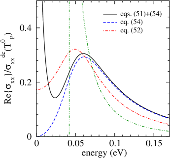
Figure 9: The mean-field single-particle conductivity of the Peierls CDW model along the highly conducting direction $x$, at temperature $T=160$ K. The bare electron dispersion is $\varepsilon({\bf k})=-\sum_{\alpha=x,y}2t_{\alpha}\cos k_{\alpha}a_{\alpha}$, with $2t_{a}=0.5$ eV and $2t_{b}=50$ meV. The mean-field transition temperature is assumed to be $T_{\rm P}^{0}=200$ K and $\Delta(160\,{\rm K})=21$ meV is the CDW order parameter at temperature $T=160$ K. The damping energies are $5\hbar\Gamma_{1}=\hbar\Gamma_{2}=30$ meV at $T<T_{\rm P}^{0}$, and $\hbar\Gamma^{0}_{1}=30$ meV at $T>T_{\rm P}^{0}$. The dot-dot-dashed line shows the inverse square-root singularity in $\sigma^{\rm inter,sp}_{xx}(\omega)$ associated with the limit $\hbar\Gamma_{2}\rightarrow 0$.

In the next section, we shall examine the Lorentz local field corrections in the relaxation-time approximation, starting with $\sigma^{\rm inter,0}_{\alpha\alpha}({\bf q},\omega)$ given by (54). The damping energy $\hbar\Gamma_{2\alpha}({\bf k})\approx\hbar\Gamma_{2\alpha}$ is assumed to be small in comparison with the interband threshold energy.

VIII Local field effects

Most Q1D systems are characterized by a large number of atoms in the unit cell (for example, in the blue bronze K_0.3MoO₃ we have 86 atoms per unit cell). The bands in the vicinity of the Fermi level are thus built of different molecular orbitals of the well-defined symmetry with the intermolecular distance large when compared to the first-neighbor atom-atom distance. Therefore, the bands are narrow and the typical interband threshold energy is in the infrared part of the spectrum. In most cases of interest, the low-energy interband electron-hole excitations are local and correspond to dipolar transitions between one molecular orbital of the $s$ symmetry and another of the $p_{\alpha}$ symmetry. Consequently, to determine the proper structure of the total conductivity tensor $\sigma_{\alpha\alpha}({\bf q},\omega)$ in this case, it is important to take into account the local field effects too.

This is not the only Q1D case in which the local field corrections are important. In the ordered state of the strong bond-CDW systems the interband dipole excitations are also local. Finally, the ordinary $sp_{\alpha}$ models with the interband threshold energy in the visible part of the spectrum also have $\sigma^{\rm inter,0}_{\alpha\alpha}({\bf q},\omega)$ of the form (54), with the dipole vertex $P_{\alpha}^{L^{\prime}L}({\bf k})\approx P_{\alpha}^{L^{\prime}L}$ real. Wooten72 ; Adler62 ; Wieser62

VIII.1 Multicomponent random-phase approximation

To demonstrate the usual procedure for dealing with the local field corrections, Adler62 ; Wieser62 ; Zupanovic96 we consider the model with the intraband currents and with one type of bound charges. We assume that the contribution of the bound charges is related to the intra-atomic or intramolecular dipolar transitions in $\sigma^{\rm inter,0}_{\alpha\alpha}({\bf q},\omega)$. In section 8.2, we shall briefly discuss the case of infrared-active optical phonons, as well. In this section, we make a simple modification of the notation. For example, the label intra is replaced by c and the label inter by b (for conduction and bound charges).

The bare intraband dielectric susceptibility is assumed to be of the form

$$\chi^{\rm c,0}({\bf q},\omega)\equiv\chi^{0}_{11}({\bf q},\omega)=(q_{\alpha}^{2}/{\rm i}\omega)\sigma^{\rm c,0}_{\alpha\alpha}({\bf q},\omega),$$ (55)

with $\sigma^{\rm c,0}_{\alpha\alpha}({\bf q},\omega)$ given by (50), and the bare interband dielectric susceptibility is

$$\chi^{\rm b,0}({\bf q},\omega)\equiv\chi^{0}_{22}({\bf q},\omega)=(q_{\alpha}^{2}/{\rm i}\omega)\sigma^{\rm b,0}_{\alpha\alpha}({\bf q},\omega),$$ (56)

with $\sigma^{\rm b,0}_{\alpha\alpha}({\bf q},\omega)$ given by (54).

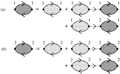
Figure 10: The RPA equations for the screened susceptibilities $\chi_{11}({\bf q},\omega)$ (a) and $\chi_{22}({\bf q},\omega)$ (b).

The electrons are assumed to be subjected to an external longitudinal electric field ${\bf E}_{0}({\bf r},t)$ represented by the scalar potential $V^{\rm ext}({\bf r},t)$. $\rho_{1}({\bf q},\omega)=\rho^{\rm c}({\bf q},\omega)$ and $\rho_{2}({\bf q},\omega)=-{\rm i}q_{\alpha}P_{\alpha}^{\rm b}({\bf q},\omega)$ are the Fourier transforms of two types of macroscopic charge densities. $\rho^{\rm c}({\bf q},\omega)$ describes the monopole-charge density of conduction electrons and $P_{\alpha}^{\rm b}({\bf q},\omega)$ the dipole-charge density of bound charges. The two-component random-phase approximation describes the long-range screening in such a case. According to figure 10, the RPA equations can be shown in the form

$$\big{[}1/\chi_{11}^{0}({\bf q},\omega)-V_{11}\big{]}\rho_{1}({\bf q},\omega)-V_{12}\,\rho_{2}({\bf q},\omega)=V^{\rm ext}({\bf q},\omega),$$

$$-V_{21}\,\rho_{1}({\bf q},\omega)+\big{[}1/\chi_{22}^{0}({\bf q},\omega)-V_{22}\big{]}\rho_{2}({\bf q},\omega)=V^{\rm ext}({\bf q},\omega).$$

(57)

Here, the $\chi_{ii}^{0}({\bf q},\omega)$ stand for two bare dielectric susceptibilities in (55) and (56), and $V_{ij}\equiv V_{ij}({\bf q})=-N_{ij}/q^{2}$ are the Fourier transforms of different long-range interactions. The numbers $N_{11}=-4\pi$, $N_{12}=N_{21}=-4\pi$ and $N_{22}=-4\pi+4\pi/3$ correspond to the monopole-monopole, monopole-dipole and dipole-dipole interactions, respectively. Zupanovic96 $N_{11}=N_{12}=N_{21}=-4\pi$ are easily shown to represent the common depolarization factors for the longitudinal ${\bf q}\approx 0$ fields. Landau95 It is not hard to verify that, after neglecting the Lorentz term $4\pi/3$ in $N_{22}$ (i.e., when $N_{22}=N_{11}$), equations (57) reduce to (53).

Equations (57) may be rewritten now in the alternative form, in terms of two dipole densities $P_{i\alpha}({\bf q},\omega)=({\rm i}/q_{\alpha})\rho_{i}({\bf q},\omega)$, to give

$$\hskip 42.67912pt\big{(}1/\alpha_{11}^{0}\big{)}P_{1\alpha}=E_{0\alpha}+N_{11}P_{1\alpha}+N_{12}P_{2\alpha},$$

$$\big{(}1/\alpha_{22}^{0}+N_{11}-N_{22}\big{)}P_{2\alpha}=E_{0\alpha}+N_{21}P_{1\alpha}+N_{11}P_{2\alpha},$$

(58)

with the implicit dependence on ${\bf q}$ and $\omega$. Here

$$\alpha^{0}_{ii}({\bf q},\omega)=(-1/q_{\alpha}^{2})\chi^{0}_{ii}({\bf q},\omega)$$ (59)

is the common notation for two bare polarizabilities. It must be emphasized that the expressions on the right-hand side of (58) represent the macroscopic electric field ${\bf E}({\bf q},\omega)$, equation (30), which is the sum of the external electric field and two depolarization fields originating from the conduction electrons and from the induced dipole moments of bound charges. Landau95 This is a useful observation which helps us to rewrite (58) in the final form

$$\big{[}1/\sigma^{\rm c}_{\alpha\alpha}({\bf q},\omega)\big{]}J^{\rm c}_{\alpha}({\bf q},\omega)=E_{\alpha}({\bf q},\omega),$$ (60)

$$\big{[}1/\alpha^{\rm b}_{\alpha\alpha}({\bf q},\omega)\big{]}P^{\rm b}_{\alpha}({\bf q},\omega)=E_{\alpha}({\bf q},\omega),$$ (61)

with

$$E_{\alpha}({\bf q},\omega)=E_{0\alpha}({\bf q},\omega)-4\pi\big{[}P_{1\alpha}({\bf q},\omega)+P_{2\alpha}({\bf q},\omega)\big{]}.$$ (62)

For the thin slab with the longitudinal polarization of the fields, the field ${\bf E}_{0}({\bf r},t)$ is identical to the dielectric displacement field ${\bf D}({\bf r},t)$ and the relation (62) leads to the usual form of the longitudinal macroscopic dielectric function. If other high-energy on-site dipolar excitations are also included, the total dielectric function becomes

$$\varepsilon_{\alpha\alpha}({\bf q},\omega)=\varepsilon^{\rm HE}_{\alpha\alpha}({\bf q},\omega)+\frac{4\pi{\rm i}\sigma^{\rm c}_{\alpha\alpha}({\bf q},\omega)}{\omega}+4\pi\alpha^{\rm b}_{\alpha\alpha}({\bf q},\omega).$$ (63)

Here, $\alpha_{11}({\bf q},\omega)=\alpha^{0}_{11}({\bf q},\omega)\equiv({\rm i}/\omega)\sigma^{\rm c}_{\alpha\alpha}({\bf q},\omega)$ and

$$\alpha_{22}({\bf q},\omega)=\frac{\alpha^{0}_{22}({\bf q},\omega)}{1-(4\pi/3)\alpha^{0}_{22}({\bf q},\omega)}\equiv\alpha^{\rm b}_{\alpha\alpha}({\bf q},\omega)$$ (64)

are two renormalized polarizabilities.

In the notation of the previous sections, this result can be expressed by (10) and (11). We can therefore conclude that the contribution of the monopole charges to the conductivity tensor is decoupled from the contribution of the dipole charges. The latter contribution is affected by the Lorentz field in the usual way, giving also the possibility for the collective contribution in $\sigma^{\rm inter}_{\alpha\alpha}({\bf q},\omega)$ when $1+(4\pi/3\omega){\rm Im}\{\sigma^{\rm inter,0}_{\alpha\alpha}({\bf q},\omega)\}=0$.

VIII.2 Infrared-active optical phonons

It was implied by our discussion of the quantum transport equation that (5), together with the density operators (3) and (23), is able to capture all relevant aspects of the electron-phonon coupling in the dynamical conductivity tensor of multiband electronic systems, at least for the scattering by acoustic and Raman-active optical phonons. In order to treat carefully infrared-active optical phonons, we must also include the direct coupling between phonons and EM fields in $H^{\rm ext}$ and take into account the corresponding local field corrections.

The generalization of (63) to such a case with multiple dipolar bound-charge contributions is very simple. For our present purposes it is simplest to replace $\alpha^{0}_{22}({\bf q},\omega)$ by the sum of all bare dipolar bound-charge polarizabilities. In the two-band case with one infrared-active phonon branch, we obtain

$$\alpha^{0}_{22}({\bf q},\omega)=(-1/q_{\alpha}^{2})\chi^{\rm inter,0}({\bf q},\omega)+\alpha^{0}_{\rm ph}({\bf q},\omega),$$ (65)

with $\alpha^{0}_{\rm ph}({\bf q},\omega)=(e^{2}/M_{\nu}V_{0})[\omega_{\nu{\bf q}}^{2}-\omega(\omega+{\rm i}\gamma)]^{-1}$ being the bare phonon polarizability.

IX Conclusions

In this article, we have derived the dynamical conductivity tensor in a general multiband electronic model with sizeable boson-mediated electron-electron interactions. Starting with the gauge-invariant form of the coupling between valence electrons and external EM fields, we have derived the general form of the self-consistent Bethe–Salpeter equations for the auxiliary intraband and interband electron-hole propagators. It is demonstrated that the intraband Bethe–Salpeter equation is identical to the usual quantum transport equation and that it reduces to the ordinary transport equation in the weak coupling limit. In this way, the present response theory of multiband electronic systems is connected to the generalized Drude formula for the intraband conductivity widely used in experimental analyses as well as to different Fermi liquid theories based on the Landau–Silin transport equations. In order to illustrate the formalism presented here, we shall give in the accompanying article KupcicJPCM the detailed description of the CDW mean-field approximation and the effects of fluctuations in the order parameter on the dynamical conductivity of the Peierls CDW systems.

References

• (1) Massidda S, Yu J and Freeman A J 1987 Phys. Lett. A 122 198
• (2) Whangbo M-H and Schneemeyer L F 1986 Inor. Chem. 25 2424
• (3) Mattheiss L F 1985 Solid State Commun. 93 791
• (4) Emery V J 1987 Phys. Rev. Lett. 58 2794
• (5) Pines D and Noziéres P 1989 The Theory of Quantum Liquids I (New York: Addison-Wesley)
• (6) Ziman J M 1972 Electrons and Phonons (London: Oxford University Press)
• (7) Ando Y, Komiya S, Segawa K and Kurita Y 2004 Phys. Rev. Lett. 93 267001
• (8) Forró L, Gaál R, Berger H, Fazekas P, Penc K, Kézsmárki I and Mihály G 2000 Phys. Rev. Lett. 85 1937
• (9) Uchida S, Ido T, Takagi H, Arima T, Tokura Y and Tajima S 1991 Phys. Rev. B 43 7942
• (10) Degiorgi L, Alavi B, Mihály G and Grüner G 1991 Phys. Rev. B 44 7808
• (11) Kézsmárki I, Mihály G, Gaál R, Barišić N, Akrap A, Forró L, Homes C C and Mihály L 2006 Phys. Rev. Lett. 96 186402
• (12) Sugai S, Suzuki H, Takayanagi Y, Hosokawa T and Hayamizu N 2003 Phys. Rev. B 68 184504
• (13) Takigawa M, Reyes A P, Hammel P C, Thompson J D, Heffner R H, Fisk Z and Ott K C 1991 Phys. Rev. B 43 247
• (14) Landau L D, Lifshitz E M and Pitaevski L P 1995 Electrodynamics of Continous Media (Oxford: Butterworth–Heinemann)
• (15) Kupčić I 2009 J. Raman Spectrosc. 40 442
• (16) Barišić S and Zelenko J 1990 Solid State Commun. 74 367
• (17) Kupčić I and Barišić S 2007 Phys. Rev. B 75 094508
• (18) Kubo R, Toda M and Hashitsume N 1995 Statistical Physics II (Berlin: Springer-Verlag)
• (19) Eliashberg G M 1961 Zh. Eksp. Teor. Fiz. 41 410 (1962 Sov. Phys. JETP 14 886)
• (20) Abrikosov A A 1988 Fundamentals of the Theory of Metals (Amsterdam: Nort-Holland)
• (21) Vollhardt D and Wölfle P 1980 Phys. Rev. B 22 4666
• (22) Götze W and Wölfle P 1972 Phys. Rev. B 6 1226
• (23) Giamarchi T 1991 Phys. Rev. B 44 2905
• (24) Kupčić I 2004 Physica B 344 27
• (25) Adler S L 1962 Phys. Rev. 126 413
• (26) Wieser N 1962 Phys. Rev. 129 63
• (27) Županović P, Bjeliš A and Barišić S 1996 Z. Phys. B 101 387
• (28) Kupčić I et al unpublished
• (29) Abrikosov A A, Gorkov L P and Dzyaloshinski I E 1975 Methods of Quantum Field Theory in Statistical Physics (New York: Dover Publications)
• (30) Dzyaloshinskii I E and Larkin A I 1973 Zh. Eksp. Teor. Fiz. 65 411 (1974 Sov. Phys. JETP 38 202)
• (31) Kupčić I, Rukelj Z and Barišić S to be published (in the main text referred to as Article II)
• (32) Fetter A L and Walecka J D 1971 Quantum Theory of Many-Particle Systems (London: McGraw–Hill)
• (33) Mahan G D 1990 Many-particle Physics (New York: Plenum Press)
• (34) Solyom J 1979 Adv. Phys. 28 201
• (35) Giamarchi T 2004 Quantum Physics in 1D (Oxford: Clarendon Press)
• (36) Vescoli V, Zwick F, Henderson W, Degiorgi L, Grioni M, Gruner G and Montgomery L K 2000 Eur. Phys. J. B 13 503
• (37) Mitrovic S, Fazekas P, Søndergaard C, Ariosa D, Barišić N, Berger H, Cloötta D, Forró L, Hóchst H, Kupčić I, Pavuna D and Margaritondo G 2007 Phys. Rev. B 75 153103
• (38) Ziman J M 1979 Principles of the Theory of Solids (London: Cambridge University Press)
• (39) Wooten F 1972 Optical Properties of Solids (New York: Academic Press)
• (40) Negele J W and Orland H 1988 Quantum Many-Particle Systems (New York: Addison–Wesley)
• (41) Kupčić I 2009 Phys. Rev. B 79 235104
• (42) Kupčić I and Barišić S 2005 Fizika A 14 47
• (43) Abrikosov A A and Genkin V M 1973 Zh. Eksp. Teor. Fiz. 65 842 (1974 Sov. Phys. JETP 38 417)
• (44) Kupčić I 2003 Physica C 391 251
• (45) Lee P A, Rice T M and Anderson P W 1974 Solid State Commun. 14 703
• (46) Kim K, McKenzie R and Wilkins J W 1993 Phys. Rev. Lett. 71 4015
• (47) Ziman J M 1988 Elements of Advanced Quantum Theory (London: Cambridge University Press)
• (48) Millis A J and Lee P A 1987 Phys. Rev. B 35 3394
• (49) Nikšić H, Tutiš E and Barišić S 1995 Physica C 241 247
• (50) Rozenberg M J, Kotliar G and Kajueter H 1996 Phys. Rev. B 64 8452
• (51) Kupčić I 2002 Physica B 322 154