Observational constraints on viable parametrizations with geometrical and dynamical probes
Abstract
We demonstrate that a wide range of viable parameterizations (including the Hu & Sawicki and the Starobinsky models) can be expressed as perturbations deviating from the CDM Lagrangian. We constrain the deviation parameter using a combination of geometrical and dynamical observational probes. In particular, we perform a joint likelihood analysis of the recent Supernovae type Ia data, the Cosmic Microwave Background shift parameters, the Baryonic Acoustic Oscillations and the growth rate data provided by the various galaxy surveys. This analysis provides constraints for the following parameters: the matter density , the deviation from CDM parameter and the growth index . We parametrize the growth index in three manners (constant, Taylor expansion around , and Taylor expansion around the scale factor). We point out the numerical difficulty for solving the generalized Friedman equation at high redshifts due to stiffness of the resulting ordinary differential equation. We resolve this problem by constructing an efficient analytical perturbative method in the deviation parameter . We demonstrate that this method is highly accurate, by comparing the resulting analytical expressions for the Hubble parameter, with the numerical solutions at low and intermediate redshifts. Surprisingly, despite of its perturbative nature, the accuracy of the method persists even for values of that are of .
pacs:
98.80.-k, 98.80.Bp, 98.65.Dx, 95.35.+d, 95.36.+x1 Introduction
A variety of cosmological studies have converged to a cosmic expansion history involving a spatially flat geometry and a cosmic dark sector formed by cold dark matter and some sort of dark energy, endowed with large negative pressure, in order to explain the observed accelerating expansion of the UniverseTeg04 ; Spergel07 ; essence ; Kowal08 ; Hic09 ; komatsu08 ; LJC09 ; BasPli10 ; komatsu11 . In this framework, the absence of a fundamental physical theory, regarding the mechanism inducing the cosmic acceleration, has given rise to a plethora of alternative cosmological scenarios. Modified gravity models act as an important alternative to the scalar-field dark energy models, since they provide an efficient way towards explaining the accelerated expansion of the universe, under a modification of the nature of gravity. Such an approach is an attempt to evade the coincidence and cosmological constant problems of the standard CDM model.
Particular attention over the last decades has been paid on gravity theories Sot10 . In this scenario of nonstandard gravity, one modifies the Einstein-Hilbert action with a general function of the Ricci scalar . The approach is a relative simple but fundamental tool used to explain the accelerated expansion of the universe. A pioneering approach was proposed long ago, where Star80 . Later on, the models were further explored from different points of view in Carrol ; FR ; Amendola-2007a and a large number of functional forms of gravity is currently available in the literature. It is interesting to mention that subsequent investigations Amendola-2007a confirmed that gravity is an unacceptable model because it fails to reproduce the correct cosmic expansion in the matter era. Of course, there are many other possibilities to explain the present accelerating stage. Indeed, in the literature one can find a variety of modified gravity models (for reviews see Refs. Ame10 ) which include the braneworld Dvali, Gabadadze and Porrati (hereafter DGP; DGP ) model, Finsler-Randers gravity Stav12 , scalar-tensor theories scal and Gauss-Bonnet gravity gauss .
The construction of observationally viable theories has proved to be challenging because it has been shown Amendola-2007a that most of these models do not predict a matter era in the cosmic expansion history. Nevertheless observationally viable models have been constructed and two such examples are the following:
-
1.
The Hu & Sawicki model Hu07 with
(1.1) where , are free parameters, is of the order of the Ricci scalar at the present time, is the Hubble constant, is the dimensionless matter density parameter at the present time, and are positive constants.
-
2.
The Starobinsky model Starobinsky-2007 with
(1.2)
These models were originally advertised as models that do not contain the cosmological constant as part of being distinct from the CDM form (where is the cosmological constant). However, it is straightforward to show that both the Hu & Sawicki and the Starobinsky models may be written in terms of CDM modified by a distortion function that depends on a deviation parameter as:
| (1.3) |
whereBamba:2012qi
| (1.4) |
for the Hu & Sawicki model with and , while
| (1.5) |
for the Starobinsky model where and . Notice that in both cases the following two limits exist for :
| (1.6) |
and therefore both models reduce to CDM for . Notice that both the Hu & Sawicki and the Starobinsky models effectively include the cosmological constant even though they were advertised as being free from a cosmological constant in the original papers Hu07 ; Starobinsky-2007 . In fact by proper choices of the function it is possible to construct infinite viable models which however will always include CDM as a limiting case for .
Thus, an important question that arises is the following: ‘What is the range of the deviation parameter that is consistent with cosmological observations?’ This is the main question addressed in the present study. Since CDM is consistent with observations we anticipate that the value is within the acceptable range of values. Thus, the interesting part of the question is ‘What is the maximum allowed value of at eg the confidence level?’
In order to address this question we solve the background modified Friedman equation assuming flatness and obtain the Hubble parameter . This involves the numerical solution of a stiff ordinary differential equation (ODE), second order in , with initial conditions at high that correspond to CDM . The numerical solution of this stiff ODE at redshifts higher than is quite challenging. However, we have developed an efficient analytical perturbative expansion in to solve it. This expansion leads to an analytic expression for to all orders in . We thus use geometric probes (type Ia surenovae, CMB shift parameter and Baryon Acoustic Oscillation data) to constrain the parameters that appear in the expression of .
In addition to geometric observations that probe directly the cosmic metric, dynamical probes play a crucial role in constraining cosmological models. The growth index, , could provide an efficient way to discriminate between modified gravity models and scalar field dark energy (hereafter DE) models which adhere to general relativity. The accurate determination of the growth index is considered one of the most fundamental tasks for Observational Cosmology. Its importance steams from the fact that there is only a weak dependence of on the equation of state parameter , as has been found by Linder & Cahn Linder2007 , which implies that one can separate the background expansion history, , constrained by geometric probes (SnIa, BAO, CMB), from the fluctuation growth history, given by . For a constant DE equation of state , it was theoretically shown that for DE models within general relativity the growth index is well approximated by (see Refs. Linder2007 ,Silv94 ,Wang98 ,Nes08 ), which boils down to for the CDM cosmology . Notice, that in the case of the braneworld model of Dvali, Gabadadze & Porrati DGP we have (see also Refs. Linder2007 ; Gong10 ; Wei08 ; Fu09 ), while for some f(R) gravity models we have for various parameter values (see Gann09 ; Tsu09 ). Recently, Basilakos & Stavrinos Bastav13 found for the Finsler-Randers cosmology.
Observationally, indirect methods to measure have also been developed (mostly using a constant ), based either on the observed growth rate of clustering Nes08 ; Guzzo08 ; Port08 ; Gong10 ; Dos10 ; Por ; Hud12 ; Bass ; Samnew12 providing a wide range of values , or on massive galaxy clusters (Vikhlinin et al. Vik09 and Rapetti et al. Rap10 ). The latter study provides . An alternative method for measuring involves weak gravitational lensing Daniel10 . Gaztanaga et al. Gazt12 performed a cross-correlation analysis between probes of weak gravitational lensing and redshift space distortions and found no evidence for deviations from general relativity. Also, Basilakos & Pouri Por and Hudson & Turnbull Hud12 imposed constraints on the growth index using the combination parameter 111Here the capital denotes the growth rate of structure. We follow the latter notation in order to avoid confusion with the ., of the growth rate of structure multiplied by the redshift-dependent rms fluctuations of the linear density field, . The above authors found Por Hud12 while Basilakos & Pouri Por showed that the current growth data can not accommodate the Dvali, Gabadadze & Porrati DGP gravity model.
In order to impose constraints on the viable models discussed above, we use in addition to geometric probes, the recent growth rate data as collected by Nesseris & Garcia-Bellido NesGa12 , Hudson & Turnbull Hud12 and Beutler et al. Beutler .
The plan of the paper is as follows. Initially in section II, we briefly discuss the background cosmological equations. The basic features of the growth index are presented in section III, where we extend the original Polarski & Gannouji method Pol for a general family of parametrizations as well as cosmological models. In section IV, a joint statistical analysis based on the Union 2.1 set of type Ia supernovae (SnIa Suzuki:2011hu ), the observed Baryonic Acoustic Oscillations (BAOs Perc10 ), the shift parameter of the Cosmic Microwave Background (CMB komatsu11 ), and the observed linear growth rate of clustering, measured mainly from the PSCz, 2dF, VVDS, SDSS, 6dF, 2MASS, BOSS and WiggleZ redshifts catalogs, is used to constraint the growth index model free parameters. Finally, we summarize our main conclusions in section V.
2 The background evolution
First of all we start with the assumption that the universe is a self-gravitating fluid described by a modified gravity namely Sot10 , and endowed with a spatially flat homogeneous and isotropic geometry. In addition, we also consider that the universe is filled by non-relativistic matter and radiation. The modified Einstein-Hilbert action reads:
| (2.1) |
where is the Lagrangian of matter, is the Lagrangian of radiation and . Now varying the action with respect to the metric222We use the metric i.e. the Hilbert variational approach. we arrive at
| (2.2) |
where is the Ricci scalar, , is the Einstein tensor and is the energy-momentum tensor of matter. Modeling the expanding universe as a perfect fluid that includes radiation and cold dark matter with velocity , we have , where and are the total energy density and pressure of the cosmic fluid respectively. Note that is the matter density, denotes the density of the radiation and , are the corresponding pressures. Assuming negligible interaction between non-relativistic matter and radiation the Bianchi identity (which insures the covariance of the theory) leads to the matter/radiation conservation laws:
| (2.3) |
the solutions of which are and . Note that the over-dot denotes derivative with respect to the cosmic time , is the scale factor and is the Hubble parameter.
Now, in the context of a flat FLRW metric with Cartesian coordinates
| (2.4) |
the Einstein’s tensor components are given by:
| (2.5) |
Inserting Eqs.(2.5) into the modified Einstein’s field equations (2.2), for comoving observers, we derive the modified Friedmann’s equations
| (2.6) |
| (2.7) |
where and . Also, the contraction of the Ricci tensor provides the Ricci scalar
| (2.8) |
Of course, if we consider then the field equations (2.2) boil down to the nominal Einstein’s equations a solution of which is the Einstein de Sitter model. On the other hand, the concordance cosmology is fully recovered for . We would like to stress here that within the context of the metric formalism the above cosmological models must obey simultaneously some strong conditions (for an overall discussion see Ame10 ). Briefly these are: (i) for , where is the Ricci scalar at the present time. If the final attractor is a de Sitter point we need to have for , where is the Ricci scalar at the de Sitter point, (ii) for , (iii) for and finally (iv) at .
Finally, from the current analysis it becomes clear that unlike the standard Friedmann equations in Einstein’s general relativity the modified equations of motion (2.6) and (2.7) are complicated and thus it is difficult to solve them analytically. Below, we are going to compare the results with those of the concordance CDM model. This can help us to understand better the theoretical basis of the current models as well as the variants from general relativity. For practical reasons (see below), we derive the the effective (“geometrical”) dark energy EoS parameter in terms of (see Ame10 ; Saini00 and references therein)
| (2.9) |
where
| (2.10) |
Differentiating the latter and utilizing Eq. (2.9) we find that
| (2.11) |
In the case of the traditional CDM cosmology , the corresponding dark energy EoS parameter is strictly equal to and the normalized Hubble function in the matter era is given by
| (2.12) |
2.1 The functional forms
In order to solve numerically the modified Friedmann equation (2.6) we need to know apriori the functional form of . Due to the absence of a physically well-motivated functional form for the parameter, there are many theoretical propositions in the literature. In this article for the background we use different reference expansion models namely flat CDM and respectively. Bellow we briefly present the two most popular models whose free parameters can be constrained from the current cosmological data.
Firstly, we use the Hu & Sawicki Hu07 model (hereafter CDM) as expressed by equation (1.1). Using the constrains provided by the violations of weak and strong equivalence principle, Capozziello & Tsujikawa CapTs found that . On the other hand it has been proposed by FuWu that is an integer number, so for simplicity in our work we have set . In Ref. Hu07 the parameters were related to , and the first derivative of at the present epoch in order to ensure the expansion history is close to that of CDM. Specifically, we have
The first two derivatives of Eq.(1.1) with respect to are
| (2.13) |
| (2.14) |
As discussed in the Introduction, the Lagrangian of Eq. (1.1) can also be written as
| (2.15) | |||||
where and . In this form it is clear that the HS model can be arbitrarily close to CDM, depending on the parameters and .
We now consider the Starobinsky Starobinsky-2007 model (hereafter CDM) as expressed by equation (1.2): As in the Hu & Sawicki Hu07 model we choose , while CapTs also showed that . In this case the and derivatives are given by
| (2.16) |
| (2.17) |
In order to ensure that the expansion history of this model is close to that of CDM we need to match the constant to , ie or
| (2.18) |
As discussed in the Introduction, the Lagrangian of Eq. (1.2) can also be written as
| (2.19) |
where and . In this form it is clear that that this model can also be arbitrarily close to CDM, depending on the parameters and . Thus, the parameter determines how close the model is to CDM.
It is interesting to mention that the above models satisfy all the strong conditions (see section II) and thus they provide predictions which are similar to those of the usual (scalar field) DE models, as far as the cosmic history (presence of the matter era, stability of cosmological perturbations, stability of the late de Sitter point etc.) is concerned. Also, we will restrict our present numerical solutions to the choice Km/s/Mpc and . For example, in this case the modified Friedmann equations for the models contain two free parameters, namely which can be constrained from the current cosmological data.
2.2 Analytic approximations
In this subsection we present a novel approximation scheme for the solution of the modified Friedmann equation (2.6) and we explicitly apply it to the two widely used models Eqs. (2.15) and (2.19).
In particular we may write eq. (2.6) as
| (2.20) |
where the prime denotes differentiation with respect to and is given by eq. (2.8). Using now eq. (1.3) for specific models, the above ODE (and its solution ) may be expanded around CDM with respect to the deviation parameter .
Since we are interested in testing deviations from the CDM model, we find it useful to perform a series expansion of the solution of the ODE (2.2) around as
| (2.21) |
where
| (2.22) |
and is the number of terms we keep before truncating the series. Usually keeping only the two first non-zero terms is more that enough to have excellent agreement of better than at all redshifts with the numerical solution for realistic values of the parameter .


By expanding Eq. (2.2) with (2.21) to any given order in we can find analytical solutions for the Hubble expansion rate. It is easy to show that for the HS model and for the first two terms of the expansion are the following:
| (2.23) |
where and are given by Eqs. (A.1) and (A.2) respectively. For the Starobinsky model for we have
Obviously, similar expressions can be obtained for any model and up to any order provided that for we obtain CDM . We stress that the expressions for are algebraic up to all orders, something that makes this method very useful and fast compared to solving the differential equation numerically. Furthermore, this method avoids another problem of the numerical integration, namely that at very high redshifts the ODE of Eq. (2.6) is quite stiff, thus making the integration impossible with standard methods. This makes the numeric solution quite time consuming and possibly unreliable, something which as we will show is not a problem for our analytic approximation.
In what follows we will test the validity of this approximation in both cases. In order to do this we compared the predictions of the analytical solutions of Eqs. (2.23) and (2.24) to the numerical solution in each case for a large variety of values for the parameter . In particular, we estimated the average percent deviation between the approximations and the numerical solution, defined as:
| (2.25) |
where the average is taken over redshifts in the range . The reason for averaging is that most of the data we will use involve distance scales, like the luminosity distance, that are integrals of the Hubble parameter. We have also kept below since the numerical ODE solver of Mathematica is unable to go to larger redshifts due to the stiffness of the ODE.
We show the results of the average error for a large variety of values of the parameter in Fig. 1. Clearly, the approximation behaves exceptionally especially within the ranges of interest, ie the vertical dashed lines. These regions correspond, as we will see in a later section, to the best fit values of . The horizontal dotted line indicates an error of . Finally, we see that our approximation is on average in agreement to better than for realistic parameters, ie , of the models. In a forthcoming paper we attempt to investigate the validity of our method against all the available gravity models.
We should note that there is some similarity between the iterative approach suggested by Starobinsky in Ref. Starobinsky:2007hu and our method. Both approaches are based on taking small deviations from an unperturbed simple case. However, our approach is based on the existence of a well defined dimensionless deviation parameter while Starobinsky uses the WKB approximation with no reference to a deviation perturbative parameter.
In addition, in Ref. Starobinsky:2007hu the iterative procedure has been based on the assumption that the Ricci scalar can be written in terms of three components namely , and (see Starobinsky’s eq.12), whereas in our approach we perform a Taylor expansion of the Hubble function around . The reason of using such an expansion is due to the fact that for close to zero both models tend to the concordance CDM model.
Our approach is indeed a perturbative approach and it should be applicable for small values of the deviation parameter . The fact that the method remains accurate even for values of of O(1) can be attributed to the fact that even for of the deviation term as a whole remains small. As expected however, the accuracy of the method decreases for increasing (see Fig. 1). We will compare the above iterative procedures in a forthcoming paper.
3 The Evolution of the linear growth factor
In this section we concentrate on the sub-horizon scales in which the DE component is expected to be homogeneous and thus we can use perturbations only on the matter component of the cosmic fluid Dave02 . Therefore, the evolution equation of the matter fluctuations, for cosmological models where the DE fluid has a vanishing anisotropic stress and the matter fluid is not coupled to other species (see Gann09 ,Lue04 ,Linder05 ,Stab06 ,Uzan07 ,Tsu08 ,Dent ), is given by:
| (3.1) |
where is the matter density and , with denoting Newton’s gravitational constant.
For those cosmological models which adhere to general relativity, [, ], the above equation reduces to the usual time evolution equation for the mass density contrast Peeb93 , while in the case of modified gravity models (see Lue04 ,Linder2007 , Tsu08 ,Gann09 ), we have (or ). Indeed it has been shown (see Refs. Gann09 ; Tsu09 ) that in the case of models the quantity is a function of the scale factor and of the wave-number
| (3.2) |
We restrict our analysis to the choice of Mpc-1 or Mpc (see also Zhang12 ).
In this context, , where is the linear growing mode (usually scaled to unity at the present time). Of course, solving Eq.(3.1) for the concordance cosmology, we derive the well known perturbation growth factor (see Peeb93 ):
| (3.3) |
In this work we use the above equation normalized to unity at the present time.
Since in most of the cases Eq.(3.1) does not yield analytical solutions, it is common in this kind of studies to provide an efficient parametrization of the matter perturbations which is based on the growth rate of clustering Peeb93
| (3.4) |
where is the growth index (see Refs. Silv94 ; Wang98 ; Lue04 ; Linder2007 ; Nes08 ) which plays a key role in cosmological studies as we described in the introduction.
3.1 The generalized growth index parametrization
Inserting the first equality of Eq.(3.4) into Eq. (3.1) and using simultaneously Eq. (2.9) and , we derive after some algebra, that
| (3.5) |
with
| (3.6) |
where in order to evaluate the final form of Eq.(3.6) we have used Eq.(2.11).
Now, we consider that the growth index varies with cosmic time. Transforming equation (3.5) from to redshift [] and utilizing Eqs.(3.4), (2.11) we simply derive the evolution equation of the growth index (see also Pol ). Indeed this is given by:
| (3.7) |
where prime denotes derivative with respect to redshift. At the present time the above equation becomes
| (3.8) |
where and .
In this work we phenomenologically parametrize by the following general relation (see Por )
| (3.9) |
Obviously, the above equation can be viewed as a first order Taylor expansion around some cosmological quantity such as , and . We would like to stress that for those functions which satisfy [or ] one can write the parameter in terms of . In this case [], using Eq.(3.1) we obtain
| (3.10) |
Let us now briefly present various forms of , .
-
•
Constant growth index (hereafter model): Here we set strictly equal to zero, thus .
-
•
Expansion around (see Pol ; hereafter model): In this case we have . Note however, that this parametrization is valid at relatively low redshifts . In the statistical analysis presented below we utilize a constant growth index, namely for .
- •
For the and parametrizations one can easily show that and , respectively. As an example, for the case of the CDM cosmology with and , Eq.(3.10) provides . In addition, based on the Starobinsky’s model with Gannouji et al. Gann09 found .
Finally, we should note that the growth index is clearly model dependent via as it can be seen by Eqs.(3.9) and (3.10). However, Gannouji et al. Ref. Gann09 found that in the case of the Starobisky model the corresponding growth rate of clustering is not really affected by the scale especially up to (see their Fig. 2). In addition, we have demonstrated that the allowed deviation from CDM is relatively small in the cases considered ( less than 0.5 at 2 in most cases) and therefore any allowed scale dependence of the growth is minor. This implies that the use of the value of the measured can be used without sacrifice of accuracy.
Another issue concerning nonlinear effects is that in this work we utilize Mpc-1 which corresponds to Mpc. Note that the power-spectrum normalization which is the rms mass fluctuation on Mpc corresponds to Mpc-1. On the other hand it has been common practice to assume that the shape of the power spectrum recovered from galaxy surveys matches the linear matter power spectrum shape on scales Mpc-1 (Smith:2002dz , Tegmark:2003uf , see also the discussion in section 4 of Percival:2006gt ). Obviously the choice of Mpc-1 insures that we are treating the liner regime. Of course we have repeated our analysis for different values of and we confirm Gannouji et al. results, ie that small variations around Mpc-1 do not really affect the qualitative evolution of the growth rate of clustering and thus of . Furthermore, we found that the evolution of is almost completely unaffected for different values of , see for example Fig. 9 (top) and Fig. 10.
Nevertheless, we do anticipate a minor contribution of non-linear effects even on these scales at a level less than a few percent Angulo:2007fw . These effects would tend to slightly amplify the value of and increase the error bars correspondingly by less than a few percent.
| Index | growth rate | Refs. | |
|---|---|---|---|
| 1 | 0.02 | Hud12 | |
| 2 | 0.067 | Beutler | |
| 3 | 0.17 | Perc04 ; Song09 | |
| 4 | 0.35 | Song09 ; Teg06 | |
| 5 | 0.77 | Song09 ; Guzzo08 | |
| 6 | 0.25 | Sam11 | |
| 7 | 0.37 | Sam11 | |
| 8 | 0.22 | Blake | |
| 9 | 0.41 | Blake | |
| 10 | 0.60 | Blake | |
| 11 | 0.78 | Blake | |
| 12 | 0.57 | Reid12 | |
| 13 | 0.30 | Tojeiro:2012rp | |
| 14 | 0.40 | Tojeiro:2012rp | |
| 15 | 0.50 | Tojeiro:2012rp | |
| 16 | 0.60 | Tojeiro:2012rp |
4 Observational constraints
In the following we briefly present some details of the statistical method and on the observational sample that we adopt in order to constrain the free parameters of the growth index, presented in the previous section.
4.1 The Growth data
The growth data that we utilize in this article based on the PSCz, 2dF, VVDS, SDSS, 6dF, 2MASS, BOSS and WiggleZ galaxy surveys, for which their combination parameter of the growth rate of structure, , and the redshift-dependent rms fluctuations of the linear density field, , is available as a function of redshift, . The estimator is almost a model-independent way of expressing the observed growth history of the universe (see Song09 ). Indeed the observed growth rate of structure () is derived from the redshift space distortion parameter and the linear bias . Observationally, using the anisotropy of the correlation function one can estimate the parameter. On the other hand, the linear bias factor can be defined as the ratio of the variances of the tracer (galaxies, QSOs etc) and underlying mass density fields, smoothed at Mpc , where is measured directly from the sample. Combining the above definitions we arrive at . We would like to point that the different cosmologies (including those of modified gravity) enter only weakly in the observational determination of (and thus of ), through the definition of distances. In Table I we quote the precise numerical values of the data points with the corresponding errors and references.
4.2 The overall Likelihood analysis
In order to constrain the cosmological parameters and the growth index of the models one needs to perform a joint likelihood analysis, involving the cosmic expansion data such as SnIa and BAO, CMB shift parameter together with the growth data. Up to now, due to the large errors of the growth data with respect to the cosmic expansion data, various authors preferred to constrain first using SnIa/BAO/CMB and then to use the growth data alone. Of course, armed with the recent high quality growth data it would be worthwhile to simultaneously constrain . In particular, we use the Union 2.1 set of 580 SnIa of Suzuki et al. Suzuki:2011hu 333The SnIa data can be found in http://supernova.lbl.gov/Union/ and in Suzuki:2011hu , and the observed BAOs. For simplicity, but without loss of generality, we only considered the case where the covariance matrix of the SnIa data is diagonal. The BAO data are given in terms of the parameter , where is the BAO scale at the drag redshift, assumed known from CMB measurements, and Perc10
| (4.1) |
is the usual volume distance.
| 6dF | SDSS | WiggleZ | ||||
|---|---|---|---|---|---|---|
| 0.106 | 0.2 | 0.35 | 0.44 | 0.6 | 0.73 | |
| 0.336 | 0.1905 | 0.1097 | 0.0916 | 0.0726 | 0.0592 | |
| 0.015 | 0.0061 | 0.0036 | 0.0071 | 0.0034 | 0.0032 | |
In this analysis we use the 6dF, the SDSS and WiggleZ BAO data shown in Table 2. The WiggleZ collaboration Blake:2011en has measured the baryon acoustic scale at three different redshifts, complementing previous data at lower redshift obtained by SDSS and 6DFGS Perc10 .
The chi-square is given by
| (4.2) |
where the indices are in growing order in , as in Table 2. For the first six points, was obtained from the covariance data in Blake:2011en in terms of :
| (4.3) |
The positions of CMB acoustic peaks are affected by the expansion history of the Universe from the decoupling epoch to today. In order to quantify the shift of acoustic peaks we use the data points of Ref. Hinshaw:2012fq (WMAP9), where and are two CMB shift parameters and is the redshift at decoupling.
For the redshift there is a fitting formula by Hu and Sugiyama Hu:1995en :
| (4.4) |
where , , , and ( correspond to the uncertainty of the Hubble parameter today, i.e. km sec-1 Mpc-1).
For a flat prior, the 9-year WMAP data (WMAP9) measured best-fit values are Hinshaw:2012fq
| (4.11) |
The corresponding inverse covariance matrix is Hinshaw:2012fq
| (4.15) |
We thus define
| (4.19) |
and construct the contribution of CMB to as
| (4.20) |
Notice that depends on the parameters (, , ). The density parameter of radiation today is
| (4.21) |
where is the photon density parameter and is the relativistic degrees of freedom. We adopt the standard values and Hinshaw:2012fq . Concerning the constraints on the parameters assuming a fixed value we should note that the statistical analysis does not depend on an a priory selected value of . First, the SnIa distance moduli are always normalized using the internally determined . On the other hand one of the merits of using the shift parameter in cosmological studies is that its dependence on the Hubble constant is almost negligible (for details see MelNes ). Indeed as it can be shown from Eq.(4.4 we use the normalized cosmological parameters and . In this context, the -dependence does it enter in the analysis of the CMB shift parameter via , but small variations around km/sec/Mpc are not expected to affect the qualitative results.


The overall likelihood function444Likelihoods are normalized to their maximum values. In the present analysis we always report uncertainties on the fitted parameters. is given by the product of the individual likelihoods according to:
| (4.22) |
where refers to the dynamical probe likelihood fit and
| (4.23) |
The vectors , contain the free parameters of the model and depend on the model. In particular, the essential free parameters that enter in the theoretical expectation are: and . Note that in the case of the CDM we have . Also, in all cases we have set .
Since likelihoods are defined as , this translates into an addition for the joint function:
| (4.24) |
with
| (4.25) |
The minimization of the was done in Mathematica™. Note that the is given by
| (4.26) |
where is the observed growth rate uncertainty.
To this end since we will use, the relevant to our case, corrected Akaike information criterion Akaike1974 , defined, for the case of Gaussian errors, as:
| (4.27) |
where , is the number of free parameters. A smaller value of AIC indicates a better model-data fit. However, small differences in AIC are not necessarily significant and therefore, in order to assess, the effectiveness of the different models in reproducing the data, one has to investigate the model pair difference AIC. The higher the value of , the higher the evidence against the model with higher value of , with a difference AIC indicating a positive such evidence and AIC indicating a strong such evidence, while a value indicates consistency among the two comparison models. A numerical summary of the statistical analysis for the background expansion models as well as for the various parametrizations is shown in Table LABEL:tab:growth1.
At this point we should stress that in this paper we only use the shift parameter and don’t use the full CMB likelihood. The reason for this is that our analysis has demonstrated self-consistently that only small deviations from CDM are allowed. Thus the use of the shift parameter for this range of small deviations is expected to be an acceptable approximation to the more accurate (but also more complicated) full CMB likelihood approach.
Furthermore, we have decided to utilize (as many authors did in the past) the CMB shift parameter which is a valid and frequently used tool in this kind of studies, especially over the last decade. The robustness of the shift parameter was tested and discussed in RefsElgCor and it has been found that the shift parameter changes when massive neutrinos are included (which is not our case here) or when there is a strongly varying equation of state parameter (the models remain close to CDM).
4.2.1 Constant growth index
First of all we utilize the parametrization (, : see section 3A). Therefore, the corresponding CDM and CDM statistical vectors contain only three free parameters namely, where . Accordingly, if we consider the CDM model then , implying that the vector includes two free parameters.
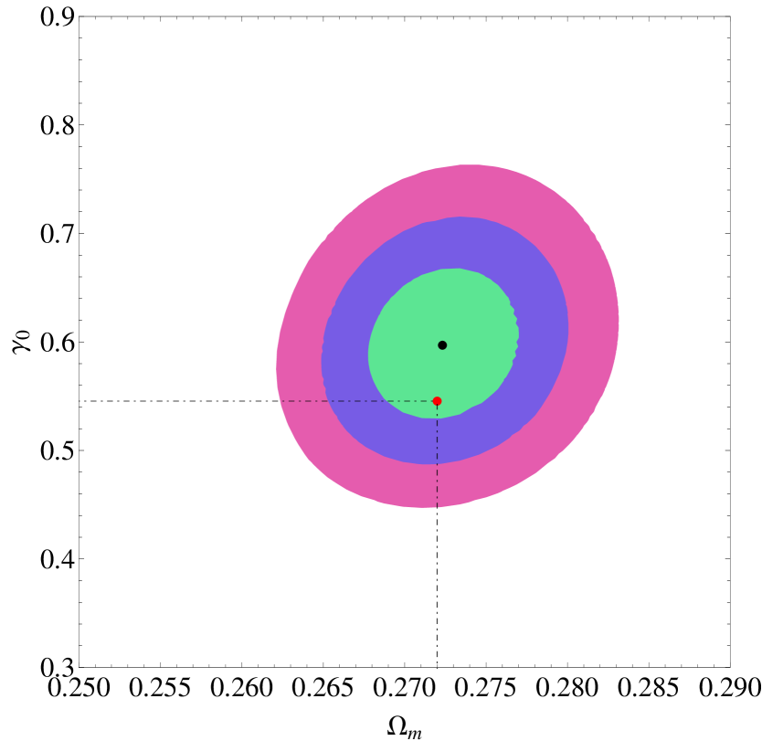
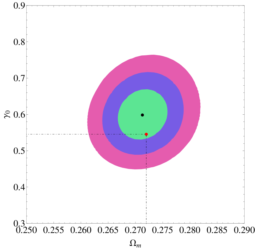
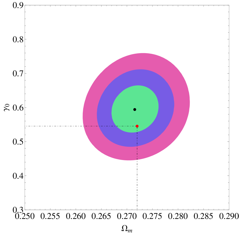
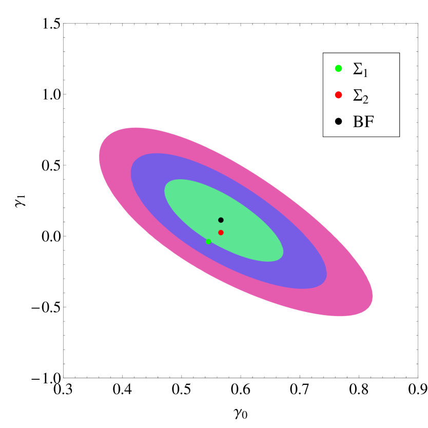
Our main results are listed in Table LABEL:tab:growth1, where we quote the best fit parameters with the corresponding 1 uncertainties, for three different expansion models. In Figure 2 we present the 1, 2 and confidence levels in the plane. It becomes evident that using the most recent growth data-set together with the expansion cosmological data we can place strong constraints on . In all cases the best fit value is in a very good agreement with that provided by WMAP9+SPT+ACT (; Hinshaw et al. Hinshaw:2012fq ).
| Exp. Model | Param. Model | AIC | ||||||
|---|---|---|---|---|---|---|---|---|
| CDM | 574.227 | 578.227 | 0 | |||||
| 573.861 | 579.861 | 1.634 | ||||||
| 573.767 | 579.767 | 1.540 | ||||||
| CDM-Hu07 | 0 | 573.855 | 579.855 | 1.628 | ||||
| 573.633 | 581.633 | 3.406 | ||||||
| 573.585 | 581.585 | 3.358 | ||||||
| CDM-Starobinsky-2007 | 0 | 580.178 | 1.951 | |||||
| 581.857 | 3.630 | |||||||
| 581.765 | 3.538 |
Concerning the CDM expansion model (see the right panel of Fig.2) our growth index results are in agreement within errors, to those of Samushia et al. Sam11 who found and to those of Bass who obtained and . However, our best-fit value is somewhat greater from the theoretically predicted value of (see lines in the right panel of Fig. 2). Such a small discrepancy between the theoretical CDM and observationally fitted value of has also been found by other authors. For example, Di Porto & Amendola Port08 obtained , Gong Gong10 measured while Nesseris & Perivolaropoulos Nes08 , found . Recently, Basilakos & Pouri Por and Hudson & Turnbull Hud12 using a similar analysis found and respectively. In this context, Samushia et al. Samnew12 obtained .


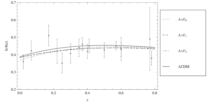
Concerning the CDM model (see the middle panel of Fig. 2) the best fit parameter is with . Also, we checked the case where , compare the middle plot of Fig. 2 with Fig. 3, and we found that our results remain mostly unaffected. Thus throughout the rest of the paper we adopt . Also in the case of Starobinsky’s CDM model (see Fig. 2) the best fit parameter is with . In Figure 4, we plot the measured with the estimated growth rate function, . The value of AICΛ() is smaller than the corresponding values which indicates that the CDM model () appears now to fit better than the CDM and CDM gravity models the expansion and the growth data. The = values (ie., ) indicate that the growth data are consistent with the CDM and CDM gravity models with a constant growth index.
At this point we should mention that in all our contour plots, eg Fig. 2, we have fixed the various parameters to the best-fit values instead if marginalizing over them. It is well known in the literature, see for example Akrami:2010cz , that marginalizing over the nuisance parameters and fixing the parameter in general gives different effects since in the former case due to the integration of the likelihood points away from the best-fit and well within the tail of the distribution will contribute in the contour, thus creating a sort of a volume effect.
4.2.2 Time varying growth index
Now we concentrate on the parametrizations, presented in section 3A. In this case the free parameters of the models are and for the CDM and CDM, CDM expansion models respectively.
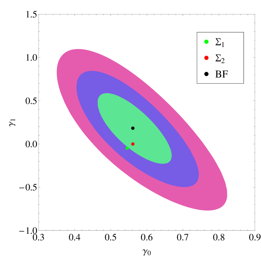
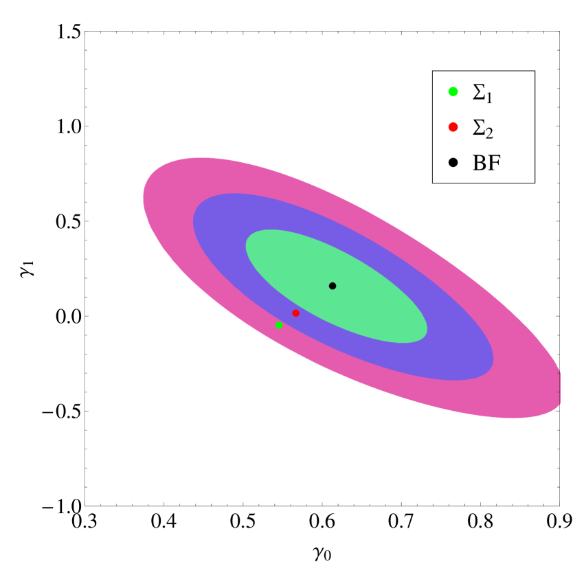
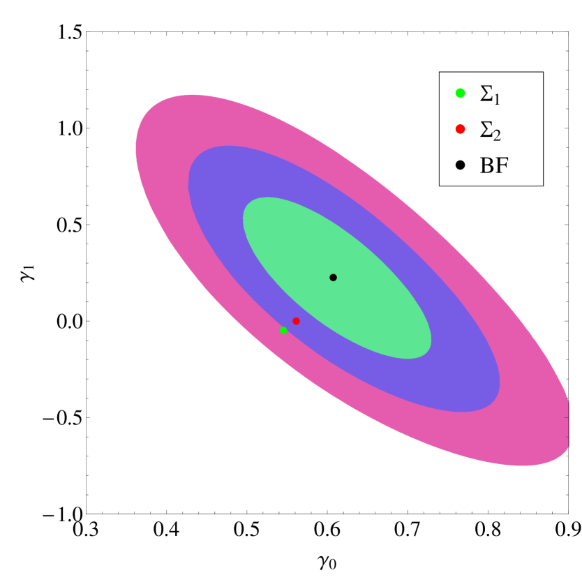
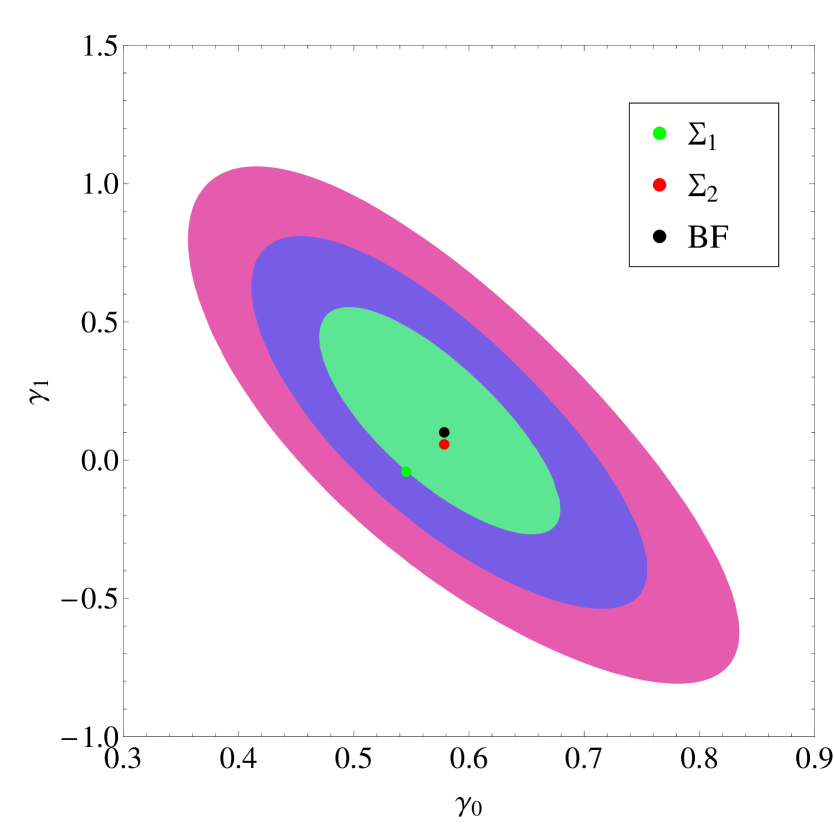
In Figure 5 (CDM model), Figure 6 (CDM model) and Figure 7 (CDM model) we present the results of our statistical analysis for the (left panel) and (right panel) parametrizations in the plane in which the corresponding contours are plotted for 1, 2 and 3 confidence levels. The theoretical values (see section 3A) in the CDM and expansion models indicated by the colored dots. Overall, we find that the predicted CDM, CDM and CDM solutions of the parametrizations are close to the borders (; see green sectors in Figs. 5, 6 and 7).
Furthermore, we also show the corresponding contours by marginalizing over the other parameters, see the bottom row in Fig. 5, and we find that both procedures are in good agreement within . Statistically this means that the likelihood function is close to being a Gaussian.
Below we briefly discuss the main statistical results: (a) parametrization: For the usual cosmology the likelihood function peaks at and with . The latter results are in agreement with previous studies Port08 ; Nes08 ; Dos10 ; Por . In the case of the CDM and CDM gravity models we find that ) with and ) and with respectively.
(b) parametrization: The best fit values are: (i) for CDM we have , (), (ii) in the case of CDM model we obtain , () and (iii) for CDM gravity model we find , ().
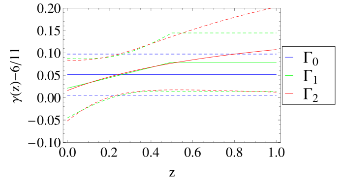
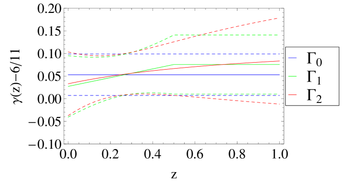
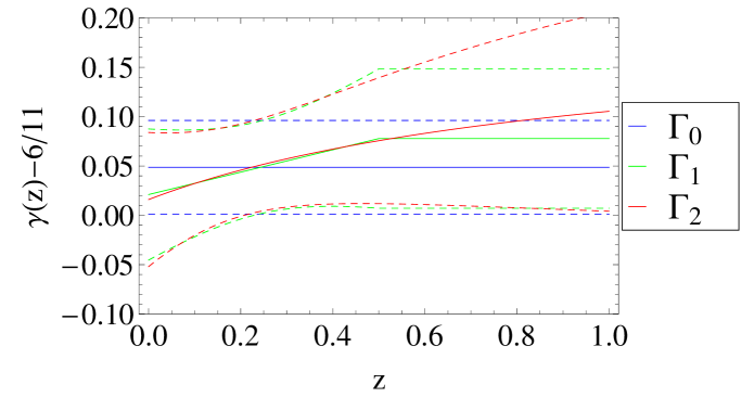
Finally, as we have already mentioned in Table LABEL:tab:growth1, one may see a more compact presentation of our statistical results. In Figure 8 we present the evolution of the growth index for various parametrizations. In the all three cases of the concordance and CDM cosmological models (see upper and bottom panels of Fig.8) the relative growth index difference of the various fitted models indicates that the parametrizations have a very similar redshift dependence for , while the parametrization shows very large such deviations for . Based on the CDM gravity model (middle panel of Fig.8) we observe that the parametrizations provide a similar evolution of the growth index.
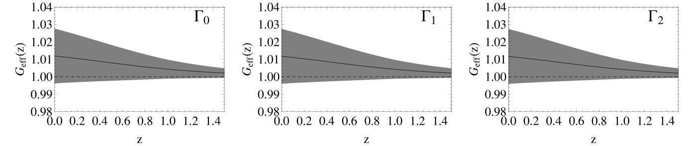
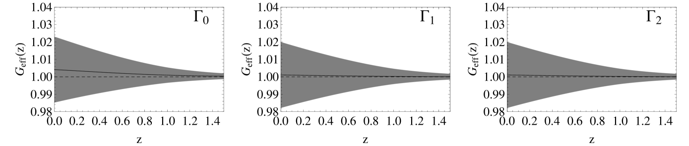
Furthermore, in Fig. 9 we show the evolution of for the two models considered in the text, CDM (left) and CDM (right). The lines correspond to (blue), (green), and (red). As it can be seen, both cases predict little evolution for at late times, around for CDM and for CDM. Furthermore, while shows almost the same evolution for all three parameterizations of CDM, this is not the case for CDM where differs significantly from the other two.
Finally, we repeated our analysis by treating as a free parameter and the corresponding results are in good agreement with our previous analysis within with the results of Table LABEL:tab:growth1, thus justifying our choice to fix . Specifically, we found:
In the case of the CDM:
-
•
for the model: , , , .
-
•
for the model: , , , , .
-
•
for the model: , , , , .
In the case of the CDM:
-
•
for the model: , , , , .
-
•
for the model: , , , , , .
-
•
for the model: , , , , , .
In the case of the CDM:
-
•
for the model: , , , , .
-
•
for the model: , , , , , .
-
•
for the model: , , , , , .
5 Conclusions
It is well known that the growth index plays a key role in cosmological studies because it can be used as a useful tool in order to test Einstein’s general relativity on cosmological scales. In this article, we utilized the recent growth rate data provided by the clustering, measured mainly from the PSCz, 2dF, VVDS, SDSS, 6dF, 2MASS, BOSS and WiggleZ galaxy surveys, in order to constrain the growth index. In particular, performing simultaneously a likelihood analysis of the recent expansion data (SnIa, CMB shift parameter and BAOs) together with the growth rate of structure data, in order to determine the cosmological and the free parameters of the parametrizations and thus to statistically quantify the ability of to represent the observations. We consider the following growth index parametrization [where , and ]. Overall, considering a CDM expansion model we found that the observed growth index is in agreement, within errors, with the theoretically predicted value of . Additionally, based on the Akaike information criterion we shown that for any type of the combined analysis of the cosmological (expansion+growth) data can accommodate the Hu-Sawicky and Starobinsky gravity models for small values of the deviation parameter .
Numerical Analysis Files: The Mathematica and data files used for the numerical analysis of this study may be downloaded from: http://leandros.physics.uoi.gr/fr-constraints/probes.htm .
Acknowledgements
We would like to thank J. García-Bellido, C. Blake, C.H. Chuang and I. Sawicki for very useful and enlightening discussions. S.N. acknowledges financial support from the Madrid Regional Government (CAM) under the program HEPHACOS S2009/ESP-1473-02, from MICINN under grant AYA2009-13936-C06-06 and Consolider-Ingenio 2010 PAU (CSD2007-00060), as well as from the European Union Marie Curie Initial Training Network UNILHC PITN-GA-2009-237920. This research has been co-financed by the European Union (European Social Fund - ESF) and Greek national funds through the Operational Program ”Education and Lifelong Learning” of the National Strategic Reference Framework (NSRF) - Research Funding Program: THALIS. Investing in the society of knowledge through the European Social Fund. SB acknowledges support by the Research Center for Astronomy of the Academy of Athens in the context of the program ”Tracing the Cosmic Acceleration”.
Appendix A Useful formulae
Here we provide the exact expressions of the coefficients for the HS and Starobinsky models for . In all cases is given by Eq. (2.22). For the HS model the first two terms are:
| (A.1) | |||||
| (A.2) | |||||
while for the Starobinsky model the first two terms are:
| (A.3) |
| (A.4) |
References
- (1) M. Tegmark et al., Astrophys. J. 606, 702 (2004)
- (2) D. N. Spergel et al., Astrophys. J. Suplem. 170, 377 (2007)
- (3) T. M. Davis et al., Astrophys. J. 666, 716 (2007)
- (4) M. Kowalski et al., Astrophys. J. 686, 749(2008)
- (5) M. Hicken et al., Astroplys. J. 700, 1097 (2009)
- (6) E. Komatsu et al., Astrophys. J. Suplem. 180, 330 (2009); G. Hinshaw et al., Astrophys. J. Suplem. 180, 225 (2009)
- (7) J. A. S. Lima and J. S. Alcaniz, Mon. Not. Roy. Astron. Soc. 317, 893 (2000); J. F. Jesus and J. V. Cunha, Astrophys. J. Lett. 690, L85 (2009)
- (8) S. Basilakos and M. Plionis, Astrophys. J. Lett. 714, 185 (2010)
- (9) E. Komatsu et al., Astrophys. J. Suplem. 192, 18 (2011)
- (10) T. P. Sotiriou and V. Faraoni, Rev. Mod. Phys. 82 451 (2010)
- (11) A. A. Starobinsky, Phys. Lett. B, 91, 99 (1980)
- (12) S. M. Carrol, V. Duvvuri, M. Trodden and M. S. Turner, Phys. Rev. D., 70, 043528 (2004)
- (13) A. D. Dolgov and M. Kawasaki, Phys. Lett. B 573, 1 (2003); T. Chiba, Phys. Lett. B 575,1 (2003); G. Allemandi, A. Borowiec, M. Francaviglia and S. D. Odintsov, Phys. Rev. D 72, 063505 (2005); A. L. Erickcek, T. L. Smith, and M. Kamionkowski, Phys. Rev. D 74, 121501 (2006); T. Chiba, T. L. Smith and A. L. Erickcek, Phys. Rev. D 75, 124014 (2007); W. Hu and I. Sawicki, Phys. Rev. D 76, 064004 (2007); S. A. Appleby and R. A.. Battye, Phys. Lett. B 654,7 (2007); J. Santos, J. S. Alcaniz, F. C. Carvalho and N. Pires, Phys. Lett. B 669, 14 (2008); J. Santos and M. J. Reboucas, Phys. Rev. D 80, 063009 (2009); V. Miranda, S. E. Joras, I. Waga and M. Quartin, Phys. Rev. Lett. 102, 221101 (2009); S. H. Pereira, C. H. G. Bessa and J. A. S. Lima, Phys. Lett. B 690 103 (2010); R. Reyes et al., Nature 464, 256 (2010); S. Capozziello, V. F. Cardone and V. Salzano, Phys. Rev. D 78, 063504 (2008) [arXiv:0802.1583 [astro-ph]]; A. Aviles, A. Bravetti, S. Capozziello and O. Luongo, arXiv:1210.5149 [gr-qc]; S. Capozziello and M. De Laurentis, Phys. Rept. 509, 167 (2011) [arXiv:1108.6266 [gr-qc]].
- (14) L. Amendola, D. Polarski and S. Tsujikawa, Phys. Rev. Lett. 98, 131302 (2007); L. Amendola, R. Gannouji, D. Polarski and S. Tsujikawa, Phys. Rev. D 75, 083504 (2007)
- (15) E. J. Copeland, M. Sami and S. Tsujikawa, Intern. Journal of Modern Physics D, 15, 1753,(2006); L. Amendola and S. Tsujikawa, Dark Energy Theory and Observations, Cambridge University Press, Cambridge UK, (2010); R. R. Caldwell and M. Kamionkowski, Ann.Rev.Nucl.Part.Sci., 59, 397 (2009); I. Sawicki and W. Hu, Phys. Rev. D., 75, 127502 (2007)
- (16) G. Dvali, G. Gabadadze and M. Porrati, Phys. Lett. B., 485, 208 (2000)
- (17) P. C. Stavrinos, A. Kouretsis and M. Stathakopoulos, Gen.Rel.Grav., 40, 1404 (2008); J. Skalala and M. Visser, Int. J. Mod.Phys.D., 19, 1119 (2010); N. Mavromatos, S. Sarkar and A. Vergou, Phys. Lett. B., 696, 300 (2011); S. Vacaru, Int. J. Mod. Phys D., 21 1250072 (2012); M. C. Werener, Gen. Rel. Grav., 44, 3047 (2012)
- (18) J. P. Uzan, Phys. Rev. D., 59, 123510 (1999); L. Amendola, Phys. Rev. D., 60, 043501 (1999); T. Chiba, Phys. Rev. D., 60, 083508 (1999); N. Bartolo and M. Pietroni, Phys. Rev. D., 61, 023518 (2000); F. Perrotta, C. Baccigalupi and S. Matarrese, Phys. Rev. D., 61, 023507 (2000); B. Boisseau, G. Esposito-Farese, D. Polarski and A. A. Starobinsky, Phys. Rev. Lett., 85, 2236 (2000); G. Esposito-Farese and D. Polarski, Phys. Rev. D., 63, 063504 (2001); D. F. Torres, Phys. Rev. D., 66, 04522 (2002); Y. Fujii and K. Maeda, ’The Scalar-Tensor theory of gravitation, Cambridge University Press (2003).
- (19) S. Nojiri, S. D. Odintsov and M. Sasaki, Phys. Rev. D 71, 023003 (2005); Comelli, Phys. Rev. D. 72, 064018 (2005); B.M.N. Carter and I. Neupane, JCAP, 0606, 004 (2006); T. Koivisto and D.F. Mota, Phys. Lett. B., 644, 104 (2007) F. Bauer, J. Solà, H. Štefančić, JCAP, 1012 029, (2010); F. Bauer, J. Solà, H. Štefančić, Phys. Lett. B., 688 , 269 (2010)
- (20) K. Bamba, A. Lopez-Revelles, R. Myrzakulov, S. D. Odintsov and L. Sebastiani, oscillations and growth index from inflation to dark energy era,” Class. Quant. Grav. 30, 015008 (2013) [arXiv:1207.1009 [gr-qc]].
- (21) W. Hu and I. Sawicki, Phys. Rev. D., 76, 064004 (2007)
- (22) A. A. Starobinsky, JETP Lett. 86, 157 (2007)
- (23) E. V. Linder, Phys. Rev. D., 70, 023511 (2004); E. V. Linder, and R. N. Cahn, Astrop. Phys., 28, 481 (2007)
- (24) V. Silveira and I. Waga, Phys. Rev. D., 64, 4890 (1994)
- (25) L. Wang and J. P. Steinhardt, Astrophys. J. 508, 483 (1998)
- (26) S. Nesseris and L. Perivolaropoulos, Phys. Rev. D 77, 023504 (2008)
- (27) Y. Gong, Phys. Rev. D., 78 123010 (2008)
- (28) H. Wei, Phys. Lett. B., 664, 1 (2008)
- (29) Y.G. Gong, Phys. Rev. D., 78, 123010 (2008) X.-y Fu, P.-x Wu and H.-w, Phys. Lett. B., 677, 12 (2009)
- (30) R. Gannouji, B. Moraes and D. Polarski, JCAP, 62, 034 (2009)
- (31) S. Tsujikawa, R. Gannouji, B. Moraes and D. Polarski D., Phys. Rev. D., 80, 084044 (2009)
- (32) H. Motohashi, A. A. Starobinsky and J. Yokoyama J., Progress of Theoretical Physics, 123, 887 (2010)
- (33) S. Basilakos and P. Stavrinos, Phys. Rev. D., 87, 043506 (2013)
- (34) L. Guzzo et al., Nature 451, 541 (2008)
- (35) C. Di Porto and L. Amendola, Phys. Rev. D., 77, 083508 (2008)
- (36) J. Dosset, et al., JCAP 1004, 022 (2010)
- (37) S. Basilakos and A. Pouri, Mon. Not. Roy. Astron. Soc., 423, 3761 (2012)
- (38) M. J. Hudson and S. J. Turnbull, Astrophys. J. Let. 715, 30 (2012)
- (39) S. Basilakos, Intern. Journal of Modern Physics D, 21, 1250064 (2012)
- (40) L. Samushia, et al., Mon. Not. Roy. Astron. Soc., 429, 1514 (2013)
- (41) A. Vikhlinin et al. 2009, Astrophys. J., 692, 1060 (2009)
- (42) D. Rapetti, S. W. Allen, A. Mantz, and H. Ebeling, Mon. Not. Roy. Astron. Soc., 406, 179 (2010)
- (43) S. A. Thomas, F. B. Abdalla, & J. Weller, Mon. Not. Roy. Astron. Soc. 395, 197 (2009); S. F. Daniel, et al., Phys. Rev. D 81, 123508 (2010); R. Bean & M. Tangmatitham, Phys. Rev. D 81, 083534 (2010)
- (44) E. Gaztanaga et al., Mon. Not. Roy. Astron. Soc., 422, 2904 (2012)
- (45) S. Nesseris and J. Garcia-Bellido, JCAP, 11, 33 (2012)
- (46) F. Beutler, et al., Mon. Not. Roy. Astron. Soc., 423, 3430 (2012)
- (47) D. Polarski and R. Gannouji, Phys. Lett. B 660, 439 (2008)
- (48) N. Suzuki, D. Rubin, C. Lidman, G. Aldering, R. Amanullah, K. Barbary, L. F. Barrientos and J. Botyanszki et al., Astrophys. J. 746, 85 (2012)
- (49) W. J. Percival, Mon. Not. Roy. Astron. Soc., 401 2148 (2010)
- (50) T. D. Saini, S. Raychaudhury,V. Sahni, and A. A. Starobinsky, Phys. Rev. Lett., 85, 1162, (2000); D. Huterer, and M. S. Turner, Phys. Rev. D., 64, 123527 (2001)
- (51) S. Capozziello and S. Tsujikawa, Phys. Rev. D., 77, 107501 (2008)
- (52) X. Fu, P. Wu and H. Yu, Eur. Phys. J. C., 68, 271 (2010)
- (53) R. Dave, R. R. Caldwell and P. J. Steinhardt, Phys. Rev. D., 66, 023516 (2002)
- (54) A. Lue, R. Scossimarro, and G. D. Starkman, Phys. Rev. D., 69, 124015 (2004)
- (55) E. V. Linder, Phys. Rev. D., 72, 043529 (2005)
- (56) F. H. Stabenau and B. Jain, Phys. Rev. D, 74, 084007 (2006)
- (57) P. J. Uzan, Gen. Rel. Grav., 39, 307 (2007)
- (58) S. Tsujikawa, K. Uddin and R. Tavakol, Phys. Rev. D., 77, 043007 (2008)
- (59) J. B. Dent, S. Dutta and L. Perivolaropoulos, Phys. Rev. D., 80, 023514 (2009)
- (60) P. J. E. Peebles, “Principles of Physical Cosmology”, Princeton University Press, Princeton New Jersey (1993)
- (61) Wen-Shaui Zhang et al., [arXiv:1202.0892] (2012)
- (62) A. B. Belloso, J. Garcia-Bellido and D. Sapone, JCAP, 1110, 010 (2011)
- (63) C. Di Porto, L. Amendola and E. Branchini, Mon. Not. Roy. Astron. Soc. 419, 985 (2012)
- (64) M. Ishak and J. Dosset, Phys. Rev. D., 80, 043004 (2009)
- (65) W. J. Percival, et al., Mon. Not. Roy. Astron. Soc., 353, 1201 (2004)
- (66) Y-S. Song and W.J. Percival, J. Cosmol. Astropart. Phys., 10 (2009) 004
- (67) M. Tegmark et al., Phys. Rev. D 74, 123507 (2006)
- (68) L. Samushia, W. J. Percival and A. Raccanelli, [arXiv:1102.1014] (2012)
- (69) C. Blake et al., Mon. Not. Roy. Astron. Soc., 415, 2876 (2011)
- (70) B. A. Reid et al., Mon. Not. Roy. Astron. Soc., 426, 2719 (2012)
- (71) R. Tojeiro, et al., Mon. Not. Roy. Astron. Soc., 424, 2339 (2012)
- (72) C. Blake, E. Kazin, F. Beutler, T. Davis, D. Parkinson, S. Brough, M. Colless and C. Contreras et al., Mon. Not. Roy. Astron. Soc. 418, 1707 (2011)
- (73) H. Akaike, IEEE Transactions of Automatic Control, 19, 716 (1974); N. Sugiura, Communications in Statistics A, Theory and Methods, 7, 13 (1978)
- (74) O. Elgaroy & T. Multamaki, J. Cosmol. Astropart. Phys., 9 (2009) 2; P. S. Corasaniti & A. Melchiorri, Phys. Rev. D, 77 (2008), 103507
- (75) G. Hinshaw, D. Larson, E. Komatsu, D. N. Spergel, C. L. Bennett, J. Dunkley, M. R. Nolta and M. Halpern et al., arXiv:1212.5226 [astro-ph.CO].
- (76) W. Hu and N. Sugiyama, Astrophys. J. 471, 542 (1996).
- (77) A. Melchiorri et al., Phys. Rev. D., 68 (2003), 043509; S. Nesseris & L. Perivolaropoulos, J. Cosmol. Astropart. Phys., 018 (2007), 0701
- (78) R. E. Smith et al. [Virgo Consortium Collaboration], Mon. Not. Roy. Astron. Soc. 341, 1311 (2003) [astro-ph/0207664].
- (79) M. Tegmark et al. [SDSS Collaboration], Astrophys. J. 606, 702 (2004) [astro-ph/0310725].
- (80) W. J. Percival, R. C. Nichol, D. J. Eisenstein, J. A. Frieman, M. Fukugita, J. Loveday, A. C. Pope and D. P. Schneider et al., Astrophys. J. 657, 645 (2007) [astro-ph/0608636].
- (81) R. Angulo, C. M. Baugh, C. S. Frenk and C. G. Lacey, Mon. Not. Roy. Astron. Soc. 383, 755 (2008) [astro-ph/0702543].
- (82) A. A. Starobinsky, JETP Lett. 86, 157 (2007) [arXiv:0706.2041 [astro-ph]].
- (83) Y. Akrami, C. Savage, P. Scott, J. Conrad and J. Edsjo, JCAP 1107, 002 (2011) [arXiv:1011.4297 [hep-ph]].