Dimethyl ether in its ground state, $\varv=0$, and lowest two torsionally excited states, $\varv_{11}=1$ and $\varv_{15}=1$, in the high-mass star-forming region G327.3-0.6

Abstract

Context. One of the big questions in astrochemistry is whether complex organic molecules are formed in the gas phase after evaporation of the icy mantles of interstellar dust grains or at intermediate temperatures within these icy mantles. Dimethyl ether (CH₃OCH₃) is one of these species that may form through either of these mechanisms, but it is yet unclear which is dominant.

Aims. The goal of this paper is to determine the respective importance of solid state vs. gas phase reactions for the formation of dimethyl ether. This is done by a detailed analysis of the excitation properties of the ground state and the torsionally excited states, $\varv_{11}=1$ and $\varv_{15}=1$, toward the high-mass star-forming region G327.3-0.6.

Methods. With the Atacama Pathfinder EXperiment 12 m submillimeter telescope, we performed a spectral line survey toward G327.3-0.6 around 1.3, 1.0, and 0.9 mm as well as at 0.43 and 0.37 mm. The observed CH₃OCH₃ spectrum is modeled assuming local thermal equilibrium.

Results. CH₃OCH₃ has been detected in the ground state, $\varv=0$, and in the torsionally excited states $\varv_{11}=1$ and $\varv_{15}=1$, for which lines have been detected here for the first time. The emission is modeled with an isothermal source structure as well as with a non-uniform spherical structure. In the isothermal case two components at 80 and 100 K are needed to reproduce the dimethyl ether emission, whereas an abundance jump at 85 K or a model with two abundance jumps at 70 and 100 K fit the emission equally well. The emission from the torsionally excited states, $\varv_{11}=1$ and $\varv_{15}=1$, is very well fit by the same model as the ground state.

Conclusions. For non-uniform source models one abundance jump for dimethyl ether is sufficient to fit the emission, but two components are needed for the isothermal models. This suggests that dimethyl ether is present in an extended region of the envelope and traces a non-uniform density and temperature structure. Both types of models furthermore suggest that most dimethyl ether is present in gas that is warmer than 100 K, but a smaller fraction of 5% –28% is present at temperatures between 70 and 100 K. The dimethyl ether present in this cooler gas is likely formed in the solid state, while gas phase formation probably is dominant above 100 K. Finally, the $\varv_{11}=1$ and $\varv_{15}=1$ torsionally excited states are easily excited under the density and temperature conditions in G327.3-0.6 and will thus very likely be detectable in other hot cores as well.

1 Introduction

A key stage in high-mass star-formation is the hot molecular core phase, in which high abundances of complex organic molecules are found in the inner warm regions (e.g. Rodgers & Charnley, 2003). The origin of complex organic species is still debated, in particular, which species are formed by solid state reactions in the cooler stages, and which form in the gas phase after evaporation of icy grain surfaces, when the young forming high-mass star starts heating up its surroundings (Tielens & Charnley, 1997; Charnley et al., 1992; Charnley, 1995). CH₃OCH₃ (dimethyl ether) is one of these “hot core molecules” for which the exact formation mechanism is not yet clear. It has frequently been detected toward high-mass star-forming regions and has a typical abundance of 10^-8–10^-7 with respect to H₂ (see e.g., Sutton et al., 1995; Nummelin et al., 2000; Schilke et al., 2001; Comito et al., 2005). It has been observed towards low-mass star-forming regions as well (Cazaux et al., 2003; Jørgensen et al., 2005a).

A recent discussion of CH₃OCH₃ formation is given by Peeters et al. (2006). Two alternative formation mechanisms are suggested: grain surface reactions and warm gas phase chemistry. In the first route, large quantities of CH₃OCH₃ may be produced by the combination of radicals formed as the photo-dissociation products of organic molecules on the surfaces of icy grains (Garrod et al., 2008). Since these radicals are mobile only at intermediate ice temperatures or higher, CH₃OCH₃ is formed above 30 K. It evaporates before H₂O and CH₃OH, due to its inability to form hydrogen bonds. In laboratory experiments by Öberg et al. (2009) an evaporation temperature of 85–90 K is found. However, the total number of desorbed molecules is a function of both temperature and time. Therefore the expected evaporation temperature of CH₃OCH₃ for more realistic warm-up time scales for star-forming regions, e.g., 10⁴–10⁶ yr for an envelope warming up from 20 to 200 K (Garrod et al., 2008), is expected to be around 70 K (see e.g., Bisschop et al., 2006, where this time scale effect is demonstrated for CO and N₂). After evaporation it is destroyed and/or protonated (Peeters et al., 2006). This results in a decreasing abundance over time and a peak in the CH₃OCH₃ abundance early in the evolution of the hot core. The second route is gas phase formation of CH₃OCH₃ from CH₃OH. This reaction has been measured in the laboratory by Karpas & Mautner (1989) and occurs in two steps. The first step is the self-alkylation of protonated methanol: CH₃OH${}_{2}^{+}\leavevmode\nobreak\ +\leavevmode\nobreak\ {\rm CH}_{3}{\rm OH}\rightarrow{\rm CH}_{3}$OCH${}_{4}^{+}\leavevmode\nobreak\ +\leavevmode\nobreak\ {\rm H}_{2}{\rm O}$. The second step is dissociative recombination, which leads to the neutral dimethyl ether. Hamberg et al. (2010) report that the dissociative recombination of CD₃OCD${}_{4}^{+}$ leads to the formation of deuterated dimethyl ether in about 7% of the cases. If the same branching ratio holds for the non-deuterated species, this means that the expected gas phase abundance ratio CH₃OCH₃/CH₃OH is probably not higher than $\sim$7%. The abundance of CH₃OCH₃ formed in the gas phase is expected to peak at higher temperatures compared to the grain-surface formation scenario, since CH₃OH only evaporates at around 100 K (Viti et al., 2004). However, low abundances of two orders of magnitude less of CH₃OH are also found in the outer parts of low-mass protostars and even cold dark clouds (Jørgensen et al., 2005b; Maret et al., 2005; Dickens et al., 2000). If this is also the case for high-mass star-forming regions, it may also lead to the formation of a small amount of dimethyl ether at low temperatures in the gas phase. In summary, CH₃OCH₃ is mainly expected to be present in the hot core and the emission should be very well modeled with one or two temperature components. One of the main questions we would like to answer in this paper is whether this is indeed is the case.

The detailed study of CH₃OCH₃ is part of a larger project in which we obtained a large, unbiased, line-survey of the 230, 290, 345, 690 and 810 GHz atmospheric windows with the Atacama Pathfinder EXperiment (APEX) telescope for the chemically extremely rich high-mass star-forming region G327.3-0.6 (Bisschop et al. in prep). The G327.3-0.6 hot core is located in an active region of high-mass star-formation, close to two HII regions, and its formation may have been triggered by an expanding infrared bubble (Minier et al., 2009). North of the “hot core” there is a colder cloud core detected in CO and N₂H⁺ (Wyrowski et al., 2006). Recent observations of mid-J CO-lines by Leurini et al. (2012) show that the molecular emission is extended and suggest that smaller high density clumps are also present in the region. The aim of our large unbiased line-survey of the high-mass star-forming region G327.3-0.6 is to make an inventory of the chemical composition of the “hot core” and to compare their abundances and excitation properties to astrochemical models of gas and grain-surface chemistry (as for example shown for ethyl formate and n-propyl cyanide by Belloche et al., 2009). Hereby we aim to get a better understanding of the chemical mechanisms, e.g., which species may be formed on grain surfaces and which in the gas phase. G327.3-0.6 is very suitable for such a study since the emission lines are strong and narrow. There is relatively little line blending, which makes it possible to detect many weaker transitions. Next to the detection of dimethyl ether, a large number of other complex organic molecules have been detected in this source, such as C₂H₅CN and CH₃C(O)CH₃ (Gibb et al., 2000, Bisschop et al. in prep.). Currently, we have detected 44 molecular species in this source, 51 isotopologues and 23 vibrationally excited states of which two are detected for minor isotopologues. Papers in which the full CHAMP⁺ and SHeFI surveys will be presented are in preparation.

This paper is structured as follows: Sect. 2 discusses the observations, Sect. 3 presents the analysis methods, Sect. 4 describes the results of the observations, and discusses the results of radiative transfer models for the dimethyl ether emission with either an isothermal or non-uniform density and temperature structure, in Sect. 5 the isothermal and non-uniform source structure models are compared and the resulting constraints on the formation mechanisms of CH₃OCH₃ are discussed, and finally Sect. 6 summarizes the main conclusions.

2 Observations

Table 1: Overview of the observed frequencies, half-power beam widths ($HPBW$) and the telescope beam efficiencies ($B_{\rm eff}$).

$\lambda$	$\nu$	Freq. range	$HPBW$	$B_{\rm eff}$
mm	GHz	GHz	″
1.3	230	213–267.5	27.1	0.81
1.0	290	270–315	21.5	0.73
0.9	345	335–362	18.0	0.65
0.43	690	623–714.8	8.7	0.43a
0.37	810	784–831 & 843.6-852.8	7.6	0.35b

^a Measured at 661 GHz. ^b Measured at 809 GHz.

G327.3-0.6 was observed in 2008 in the 230, 290 and 345 GHz atmospheric windows with the Atacama Pathfinder EXperiment (APEX) located in the Atacama desert in Chile (Güsten et al., 2006a, b). Additional observations were performed in August 2009 in the 690 and 810 GHz atmospheric windows. The coordinates for the G327.3-0.6 hot core are $\alpha_{\mathrm{J2000}}$=15^h53^m08$\aas@@fstack{s}$2, $\delta_{\mathrm{J2000}}$=$-54^{\circ}$37$\arcmin$06.6$\arcsec$ and the source has a $V_{\mathrm{lsr}}=-$45 km s^-1. We used a distance of 2.9 kpc for G327.3-0.6 (Simpson & Rubin, 1990) and a luminosity of 1$\times$10⁵ L_⊙ (Wyrowski et al., 2006). In Table 1 the precise frequency ranges that are covered are given. The front-ends used were the SHeFI heterodyne receivers, APEX-1 for the 230 GHz window and APEX-2 for the 290 and 345 GHz windows (Vassilev et al., 2008). The 2 times 7-pixel dual channel heterodyne receiver array, CHAMP⁺ (Kasemann et al., 2006), was employed for the 690 and 810 GHz observations. The Fast Fourier Transform Spectrometer (FFTS) was the backend for all the SHeFI observations (Klein et al., 2006). It has 8192 spectral channels divided over two units, each of which has a bandwidth of 1 GHz with a channel spacing of 122 kHz. The two units are spaced such that there is 100 MHz overlap, which results in a bandwidth of 1.9 GHz covered per setting. For the CHAMP⁺ array the Array Fast Fourier Transform Spectrometer (AFFTS) was used. It has 2048 channels in each of its two units, both of which have a bandwidth of 1.5 GHz, a resolution of 732 kHz and an overlap between both units of 180 MHz. All observations were done in single sideband mode. The telescope pointing was performed on the continuum of the source itself. The pointing was checked every two hours for the SHeFI instrument and every hour for the CHAMP⁺ instrument and found to be accurate within 2”. The focus was optimized every few hours or around sun-set and sun-rise and when large temperature changes occurred. The wobbling mode with a throw of $\pm$100″ was used for the observations.

The main-beam temperatures have been calculated by:

$$T_{\rm MB}=T_{\rm A}^{\ast}\times\frac{F_{\rm eff}}{B_{\rm eff}}$$ (1)

where $F_{\rm eff}$ and $B_{\rm eff}$ are the forward and the main beam efficiencies, respectively. The main beam efficiencies were based on the measurements at a number of given frequencies: the SHeFI efficiencies are tabulated in Vassilev et al. (2008), whereas the efficiencies of the CHAMP⁺ instrument for the August 2009 observing campaign are given online All values used in this paper are shown in Table 1. These efficiencies were scaled to the efficiencies at the observing frequencies using the Ruze-formula. The half power beam widths ($HPBW$) of APEX (Güsten et al., 2006b, 2008) are given by:

$$HPBW=7.8\arcsec\frac{800}{\nu{\rm(GHz)}}.$$ (2)

The rms noise level reached on the $T_{\rm MB}$ scale at 0.244 MHz resolution was 30–40 mK for the 230 and 290 GHz bands and 45–55 mK in the 345 GHz window. For the 690 GHz and 810 GHz windows the rms was 100–200 mK and 150–500 mK, respectively, at a resolution of 0.732 MHz.

Before modeling the molecular emission of the source a zeroth order baseline was subtracted. The baseline was determined based on emission-free parts of the spectra. In general, the system temperatures calculated were averaged over the observed range of 1.8 GHz per setting. However, for the CHAMP⁺ spectra, there are a few frequency settings where strong atmospheric emission lines are present. These settings were recalibrated channel-by-channel off-line. In most cases this reduced the atmospheric features in the spectra and increased the overall calibration accuracy in the band. However, the calibration close to these strong atmospheric lines remains very uncertain and does thus not give reliable quantitative constraints. We have compared observations of the exact same frequency taken at different days and from this we estimate that the calibration uncertainty leads to an overall uncertainty on the line-strengths of 15–20% for the SheFI data and $\sim$25–30% for the CHAMP⁺ data. At 1.3, 1.0, and 0.9 mm the confusion limit is reached for a significant fraction of the observed frequency ranges, however sufficient emission free ranges were present to determine a baseline.

3 Data Analysis

This research made use of the myXCLASS program (Comito et al., 2005), which accesses the CDMS (Müller et al., 2001, 2005) and JPL (Pickett et al., 1998) molecular data bases. Additionally, we modeled selected emission lines of the ground state with the new radiative transfer tool LIME (Brinch & Hogerheijde, 2010). The line assignments for CH₃OCH₃ are based on new measurements of the ground state, $\varv=0$, by Endres et al. (2009) as well as the lowest two torsionally excited states, $\varv_{11}=1$ and $\varv_{15}=1$ (Endres et al in prep.). The $\varv_{11}=1$ and $\varv_{15}=1$ states lie 200 and 240 cm^-1, or in temperature units 288 and 346 K above the ground state, respectively. Local thermal equilibrium (LTE) models were constructed for the emission, in which the source size $\theta$ is given in $\arcsec$, column density $N_{\rm T}$ in cm^-2, rotational temperature $T_{\rm rot}$ in K, and line width $\Delta V$ in km s^-1 were varied to obtain the best-fit model by-eye. We have estimated the uncertainties by systematically varying all the parameters in the myXCLASS models. The model results are shown together with the uncertainties in Table 2. The increments with which the different parameters were varied is equal to half the uncertainty given in Table 2.

Although the myXCLASS models are used to derive the molecular parameters, rotational diagrams (see Goldsmith & Langer, 1999, for a discussion of the method) were used to assess the reliability of the fits. Rotational diagrams were constructed for the lines of the ground and torsionally excited states that were not too severely blended, meaning that these transitions are found to be the major contribution to the emission feature. Blending with known features of other molecules has been corrected for by the subtraction of the model for all molecules minus dimethyl ether from the integrated line-intensities. Under LTE conditions and assuming the emission is optically thin the integrated line intensities, $\int T_{\rm MB}dV$ in K km s^-1 are related to the column density in the upper energy level, $N_{\rm u}$ in cm^-1, divided by the degeneracy in the upper energy level, $g_{\rm u}$, by:

$$\frac{N_{\rm u,thin}}{g_{\rm u}}=\frac{8\pi k\nu^{2}\int T_{\rm MB}dV}{hc^{3}A_{\rm ul}B},$$ (3)

where $\nu$ is the transition frequency in Hz, $A_{\rm ul}$ is the Einstein $A$-coefficient in s^-1. The Einstein $A$-coefficient can be calculated through:

$$A_{\rm ul}=1.16395\cdot 10^{-20}\nu^{3}\mu^{2}S,$$ (4)

where $\mu$ is the dipole moment in Debye and $S$ is the line strength. $B$ is the beam-filling factor and is calculated through:

$$B=\frac{\theta_{\rm G327.3-0.6}^{2}}{\theta_{\rm G327.3-0.6}^{2}+\theta_{HPBW}^{2}},$$ (5)

where $\theta_{\rm G327.3-0.6}$ is the size (FWHM) of the source in arcsec, which is determined from the isothermal myXCLASS model for the optically thick transitions. If the emission for a specific transition is optically thick the integrated line intensity additionally has to be multiplied by the correction factor $C_{\tau}$, which is given by:

$$C_{\tau}=\frac{\tau}{1-e^{-\tau}},$$ (6)

where $\tau$ is the optical depth. Thus:

$$\frac{N_{\rm u,thick}}{g_{\rm u}}=\frac{N_{\rm u,thin}}{g_{\rm u}}C_{\tau}$$ (7)

In this paper the optical depths for the emission lines are calculated with the isothermal myXCLASS model. The total source-averaged column density $N_{\rm T}$ can then be computed from:

$$N_{\rm T}=\frac{N_{\rm u}}{g_{\rm u}}\frac{Q(T_{\rm rot})}{e^{-E_{\rm u}/T_{\rm rot}}},$$ (8)

where the rotational temperature, $T_{\rm rot}$, should be equal to the kinetic temperature of the gas under LTE conditions, $Q(T_{\rm rot})$ is the rotational partition function, and $E_{\rm u}$ is the upper level energy in K. Practically, this means that $T_{\rm rot}$ can be determined from the slope of the rotational diagram (such as for example shown in Fig. 2) and $N_{\rm T}$ from the intercept with the y-axis.

The fit to the data has been optimized, using an iterative approach. First we made a model that fits the data well by-eye and subsequently a rotation diagram was constructed. The results of this fit were then used as renewed input until the fit was optimal.

3.1 Critical density

One of the main assumptions in our analysis is that the emission is in LTE. In the following we will use the critical density, $n_{\rm cr}$ in cm^-3, to validate this assumption. However, it is necessary to mention that $n_{\rm cr}$ is not per definition equal to the density where the excitation temperature is equal to the kinetic temperature. This depends on for example the frequency of a transition, and the temperature of the gas (Evans, 1999, 1989). Both higher frequencies and higher temperatures decrease the densities at which a given transition is effectively thermalized. At submillimeter wavelengths the thermalization density is approximately the same as the critical density. We therefore use the critical density here to estimate the effective thermalization density. Unfortunately it is not possible to derive the critical density for transitions of dimethyl ether directly, since its collisional rates are not known. However, we can attempt to estimate them, when we assume that the rates for CH₃OH are comparable within an order of magnitude. The critical density for a transition is calculated by:

$$n_{\rm cr}=\frac{A_{\rm ul}}{\gamma\ }.$$ (9)

Here $\gamma$ is the collisional rate in cm³ s^-1. The collisional rates for CH₃OH are $\sim$10^-11–10^-10 cm³ s^-1 (Pottage et al., 2004). The values for the Einstein A-coefficients of CH₃OCH₃ range from 10^-6 s^-1 up to 4.0$\times$10^-3 s^-1 at the highest frequencies and up to 3.0$\times$10^-4 s^-1 for frequencies below 370 GHz. This means that $n_{\rm cr}$ can be as high as 10⁷–10⁸ cm^-3 for the lines with the highest line-strengths assuming the collisional rate is 10^-11 cm³s^-1. However, as previously mentioned the effective density at which a transition is thermalized is likely to be different from the critical density. Multiple effects can play a role, e.g., for transitions from moderately to highly excited states the sum over all collisional rates from the upper state need to be considered and not only the one corresponding to the radiative transition. High optical depths can also lower the density at which a transition is thermalized. Additionally, a strong infrared radiation field can thermalize the populations to the radiation field irrespective of the density. However we do not expect the latter to be a problem for dimethyl ether in this source (see Sect. 4.2). When effects like high optical depth or the inclusion of all collisional rates are taken into account, the density at which the molecular emission reflects the kinetic temperature is one or two orders of magnitude lower than the critical density, i.e., 10⁵–10⁶ cm^-3. Since we used a rather conservative estimate for the collisional rate, the effective thermalization density may be lower still. This means that most transitions should easily be thermalized at densities of 10⁶–10⁷ cm^-3 we expect at temperatures from 70 K and higher from the model by Rolffs et al. (2011).

3.2 Dust optical depth

The observations described in this paper cover a large frequency range and it is therefore important to obtain a model that is consistent over all frequencies. The LTE models constructed with the myXCLASS software systematically overestimate the line-strength for the CHAMP⁺ part of the survey. This is likely due to the dust optical depth at higher frequencies, which absorbs part of the radiation emitted by the molecules (Mezger et al., 1990). This can be corrected for by estimating the total column density of hydrogen, $N_{\rm H}$, from which the dust optical depth is calculated such that the relative intensities over all frequencies match. $N_{\rm H}$ is given by $N({\rm H})+2N({\rm H_{2}})$ in cm^-2. The dust optical depth, $\tau_{\rm d}$, is calculated by:

$$\tau_{\rm d}=N_{\rm H}\ \sigma_{\lambda}^{H},$$ (10)

The dust collisional cross section ($\sigma_{\lambda}^{\rm H}$) is given by:

$$\sigma_{\lambda}^{\rm H}=7\times 10^{-21}\ \frac{Z}{Z_{\odot}}\ b\lambda_{\rm\mu m}^{-2},$$ (11)

for $\lambda>100\leavevmode\nobreak\ \mu$m. The metallicity for G327.3-0.6, $\frac{Z}{Z_{\odot}}$, is assumed to be equal to that in the galactic center, i.e. 2, and $b$ is an adjustable factor, that takes grain properties into account. The myXCLASS program assumes a value of 3.4 for deeply embedded IR sources where the grains are expected to be coated with thin ice layers (Rengarajan, 1984). In comparison, a factor of 1.9 is used for grains without ice layers. The latter may be more correct for the CH₃OCH₃ emission that is arising from warmer gas. Furthermore in the myXCLASS program, dust is considered to be present in a foreground layer and corrected for with the factor e${}^{-\tau_{\rm d}}$. For consistency we use the same correction factor for the rotational diagram treatment. However, when the dust is present in the source itself molecular line emission is expected to be attenuated with the factor $(1-e^{-\tau_{\rm d}})/\tau_{\rm d}$. The combination of the effect of the dust grain properties and foreground/in situ treatment could lead to an underestimation of the value for $N_{\rm H}$ with a factor 4–5 in addition to the uncertainty of about $\sim$50% on the value derived from the CHAMP⁺ observations with myXCLASS. However, with the additional uncertainties on the source structure and the dust composition it is accurate enough for our purposes. The line-intensities over the full frequency range covered in this paper are corrected for by the factor e${}^{-\tau_{\rm d}}$. The optimal value for $N_{\rm H}$ is derived by assuming the model for dimethyl ether found at the lower frequencies also to hold at the higher frequencies (See Sect. 4.1). Typical values for $\tau_{\rm d}$ are 0.08 (230 GHz), 0.13 (290 GHz), 0.19 (345 GHz), 0.76 (690 GHz) and 1.04 (810 GHz).

4 Results

4.1 The CH₃OCH₃ ground state, $\varv=0$

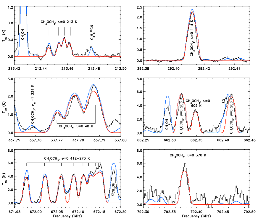
Figure 1: Selected emission lines for ground-state CH₃OCH₃, $\varv=0$, in all atmospheric windows. The observed spectrum is displayed in black, the myXCLASS isothermal model for CH₃OCH₃, $\varv=0$, in red and the myXCLASS isothermal model for all assigned species in blue. The major transitions of CH₃OCH₃, $\varv=0$, and other detected species are indicated in the plot as well as the values for $E_{\rm u}$ for the transitions of CH₃OCH₃, $\varv=0$.

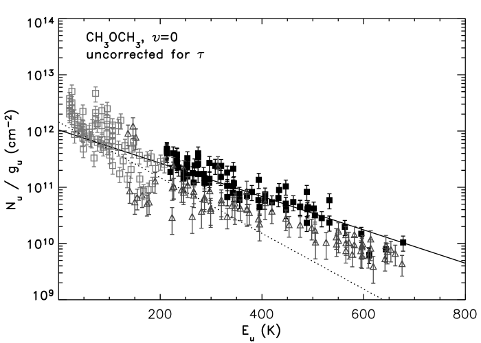
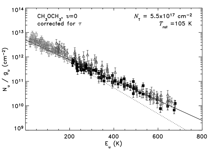
Figure 2: Rotational diagram for CH₃OCH₃, $\varv=0$, uncorrected for the predicted optical depth (left) and corrected for the optical depth (right), in all other aspects the data is treated in the same way, as well as that the same symbols and line-styles are used in both panels. Line-emission from other species, derived from an isothermal model of all identified species minus dimethyl ether, has been subtracted from the dimethyl ether emission in both figures. The filled squares ($\blacksquare$) indicate the lines with $E_{\rm u}>$ 200 K and open squares ($\Box$) lines with $E_{\rm u}<$ 200 K, detected with SHeFI in the 230, 290 and 345 GHz windows. The open triangles ($\triangle$) indicate CHAMP⁺ data. The solid line shows the least squares-fit to the $E_{\rm u}>$ 200 K data and the dotted line the least-square fit to the $E_{\rm u}<$ 200 K transitions. The dust absorption has been corrected for. $N_{\rm T}$ for the fit to the transitions with $E_{\rm u}\leavevmode\nobreak\ >$ 200 K is 5.5$\times$10¹⁷ cm^-2 and $T_{\rm rot}$ is 105 K for a source size of 2.6″. For the transitions with $E_{\rm u}\leavevmode\nobreak\ <$200 K these values are 5.0$\times$10¹⁷ cm^-2 and 82 K, respectively for a source size of 3.2″.

Emission lines for the ground state are detected in all atmospheric windows, more specifically 337 in the SHeFI bands and 136 at the frequencies observed with CHAMP⁺. Examples of lines detected for each band are shown in Fig. 1. Naturally a large number of lines is blended with transitions of other species, which results in a number of 250 features, for which CH₃OCH₃ is the main contributor (an overview of the CH₃OCH₃, $\varv=0$ transitions is given in the appendix in Table LABEL:detfreqv0). As described in Sect. 3, the model for the emission of all other assigned features is taken into account in the isothermal myXCLASS model. The values for $E_{\rm u}$ for the detected transitions range from 21.7 to 677.5 K, and are very evenly spread in energy. The optical depths for detected transitions range from 0.056 to 26.

Table 2: Resulting best by-eye fits for the isothermal myXCLASS model. The estimated uncertainties on the different parameters are given in brackets.

$\theta$	$T_{\rm rot}$	$N_{\rm T}^{a}$	$\Delta V$
″	K	cm-2	km s-1
One-component model
3.2(0.2)	90(5)	8.0$\times$1017(0.5)	4(0.3)
Two-component model
2.6(0.2)	100(5)	1.5$\times$1018(0.3)	4(0.3)
3.2(0.2)	80(5)	7.5$\times$1016(2.0)	4(0.3)
${}^{a}N_{\rm T}$ is the source averaged column density calculated using Eq. 8.

We have attempted to fit the data with both a one-component and two-component isothermal model (see Sect. 3). In general the two components fit the data better by-eye, since it is difficult to model both the intensities of the optically thick transitions with excitation temperatures above and below 200 K accurately with only one component. The optically thick lines with the lowest excitation temperatures of $\sim$30 K namely suggest a significantly larger source size compared to the optically thick lines of $\sim$200 K. To get an idea of how well both models fit we have calculated a reduced $\chi^{2}$ for both isothermal models for the same transitions as modeled with the non-uniform density model discussed in Sect. 4.3. The parameters for both models, as well as the reduced $\chi^{2}$ are shown in Table 2. The two-component isothermal model has a reduced $\chi^{2}$ of 1.34 vs. 2.08 for the one-component model. This result may suggest that there are two physical components, but could also indicate that the dimethyl ether emission arises from a region with a non-uniform density and/or temperature structure. The same is seen in the CHAMP⁺ data. Here two different values for $N_{\rm H}$ are needed to correct for the dust optical depth (see Sect. 3.2 for an explanation). This is also illustrated in Fig. 2, where the CHAMP⁺ data (shown as $\triangle$) is corrected for the $\tau_{\rm d}$ found for the highest excitation lines for a hydrogen column density of $2\times$10²⁴ cm^-2. This value is consistent within the uncertainties mentioned in Sect. 3.2 with ${N}_{T\rm>100\leavevmode\nobreak\ K}$ of 4.5$\times$10²⁴ cm^-2 derived for the models by Rolffs et al. (2011) from the 870 $\mu$m dust emission, in particular since the value found with myXCLASS (see Sect. 3.2) likely underestimates the actual value. The CHAMP⁺ detections are well fit at the highest excitation energies, but that the excitation levels below 200 K actually are corrected too much and lie above the fit and most of the transitions detected with SheFI (shown in Fig. 2 as $\Box$). These lower energy CHAMP⁺ detections thus seem to require a lower dust optical depth and corresponding hydrogen column density ($N_{\rm H}=$1$\times$10²⁴ cm^-2) to match the lower frequency data. This could be explained by dimethyl ether gas that is present in an extended region with a temperature and density gradient or that has two different abundance components. Both scenarios may well cause dimethyl ether to “see” different dust columns dependent on the location in the envelope of the star-forming region (see also Sect. 5).

The two-component isothermal myXCLASS model fit to the data is shown in the rotation diagram in Fig. 2 for the ground state. On the left the rotation diagram is shown without the correction for optical depth and on the right with the correction for the optical depth derived from the model. Least-square fits of the transitions are shown for both $E_{\rm u}$ values above 200 K (solid line) and below 200 K (dotted line). The column density for the fit to the transitions with $E_{\rm u}\leavevmode\nobreak\ >$ 200 K is 5.5$\times$10¹⁷ cm^-2 and the rotational temperature is 105 K for a source size of 2.6″. For the transitions with $E_{\rm u}\leavevmode\nobreak\ <$200 K these values are 5.0$\times$10¹⁷ cm^-2 and 82 K, respectively for a source size of 3.2″. The difference between the column densities from the rotational diagram and the two components given in Table 2 are due to the fact that the two temperature components of the isothermal model are both contributing to the emission of all transitions, and the least-square column densities are therefore higher. The comparison between the two rotation diagrams clearly shows that a large fraction of the “scatter” is due to the optical depth of the emission lines. The rotational temperature derived in the uncorrected rotational diagram is furthermore higher and the column density about an order of magnitude lower compared to that corrected for optical depth. Some scatter remains for the corrected data which is most likely due to the presence of line-blends with unidentified features, as well as uncertainties in the baseline level due to line-confusion.

As discussed in Sect. 3.1, it is possible (though not likely) that some transitions for dimethyl-ether are excited under non-LTE conditions. If we remove those lines for which this is most probable, the fit to the data is not affected significantly, and most of these transitions are very well-fit by the LTE model. Thus we conclude that LTE indeed is a good approximation for dimethyl ether in this source.

4.2 The CH₃OCH₃ torsionally excited states $\varv_{11}=1$ and $\varv_{15}=1$

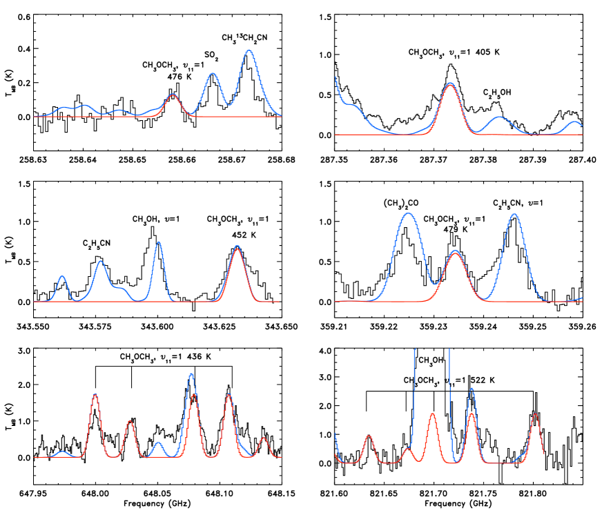
Figure 3: Selected emission lines for CH₃OCH₃, $\varv_{11}=1$, in all atmospheric windows. The observed spectrum is displayed in black, the myXCLASS isothermal model for only CH₃OCH₃, $\varv_{11}=1$, in red and the model for all assigned species in blue. Transitions of CH₃OCH₃, $\varv_{11}=1$, and other detected species are labeled in the plot as well as the values for $E_{\rm u}$ for CH₃OCH₃, $\varv_{11}=1$.

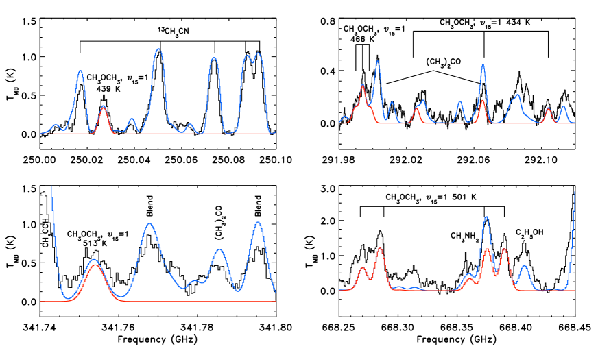
Figure 4: Selected emission lines for CH₃OCH₃, $\varv_{15}=1$ in four atmospheric windows. The observed spectrum is displayed in black, the myXCLASS isothermal model for only CH₃OCH₃, $\varv_{15}=1$, in red and the model for all assigned species in blue. Transitions of CH₃OCH₃, $\varv_{15}=1$, and other detected species are labeled in the plot as well as the values for $E_{\rm u}$ for CH₃OCH₃, $\varv_{15}=1$.

Emission from the $\varv_{11}=1$ torsionally excited state is detected in all atmospheric windows studied here. The $\varv_{15}=1$ state is detected in all atmospheric windows except for the highest (810 GHz) window. The number of lines present in the observations for $\varv_{11}=1$ with the SHeFI receiver is 117 and 84 with the CHAMP⁺ receiver. For $\varv_{15}=1$ these numbers are 59 and 39, respectively. Unfortunately, some of these features are very strongly blended with transitions of other species so that there are only 101 and 42 “clean” features that can reliably be used for the analysis of $\varv_{11}=1$ and $\varv_{15}=1$, respectively (see for an overview of these assignments Tables LABEL:detfreqv11 and LABEL:detfreqv15 in the appendix). In Figs. 3 and 4 selected transitions for both states are shown for all atmospheric windows in which they are detected. The torsionally excited states states lie $\sim$288 K ($\varv_{11}=1$) and 346 K ($\varv_{15}=1$) above the ground state. Lines with $E_{\rm u}$ up to 550 K have been detected. The smaller energy range covered compared to the ground state, means that the column densities and rotational temperatures for $\varv_{11}=1$ and $\varv_{15}=1$ lines are less well-constrained. However, their spectra are very well modeled with the same LTE model as the ground state (see Sect. 4.1). Interestingly the $\varv_{11}=1$ torsionally excited state is infrared inactive while $\varv_{15}=1$ is infrared active. If dimethyl ether would strongly interact with the infrared radiation field, a difference between the excitation of the ground state and the torsionally excited states or between the two torsionally excited states would be expected. Since this clearly is not the case, we conclude that for this specific molecule it is not necessary to include or correct for an infrared radiation field in the models.

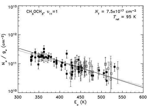
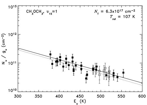
Figure 5: Rotational diagrams for the torsionally excited states, $\varv_{11}=1$ (left) and $\varv_{15}=1$ (right), of dimethyl ether. The filled squares ($\blacksquare$) indicate transitions detected with the SHeFI instrument, the open squares ($\Box$) detections with the CHAMP⁺ instrument. The solid line represents the fit to the torsionally excited states and the dotted line indicates the fit to the ground state transitions with $E_{\rm u}>$ 200 K. The least-square fit to the torsionally excited state, $\varv_{11}=1$ gives a resulting $N_{\rm T}$ of 7.5$\times$10¹⁷ cm^-2 and a $T_{\rm rot}$ of 95 K. For the torsionally excited state, $\varv_{15}=1$, these values are 6.3$\times$10¹⁷ cm^-2 and 107 K, respectively.

In Fig. 5 the rotational diagrams are shown for the $\varv_{11}=1$ and $\varv_{15}=1$ states. The least-square fits are indicated by the solid black line and a fit to the high energy transitions of the ground state is indicated with the dotted line. The least-square fit to the torsionally excited state, $\varv_{11}=1$ gives a resulting column density of 7.5$\times$10¹⁷ cm^-2 and a rotational temperature of 95 K. For the torsionally excited state, $\varv_{15}=1$, these values are 6.3$\times$10¹⁷ cm^-2 and 107 K, respectively. The consistency between the model for the ground state and the torsionally excited states is not just clear from the isothermal model fits shown in Figs. 3 and 4, but is also apparent in these rotational diagrams (Fig. 5). Due to the lower optical depths for the transitions of the excited states one could expect that the critical densities for the lines from the $\varv_{11}=1$ and $\varv_{15}=1$ states and thus the densities where LTE is a good approximation are higher than for the ground state. Nonetheless they are very well fit by the same model, confirming our conclusion in Sect. 3.1 that LTE is a good assumption for dimethyl ether toward the G327.3-0.6 star-forming region.

The optical depths in the isothermal models for the torsionally excited states range from 0.05–0.655 and 0.038–0.387 for $\varv_{11}=1$ and $\varv_{15}=1$, respectively. The line intensities are very close to what is expected based on the ground state and no lines that are expected to be there are missing. We are therefore confident, that we have detected the $\varv_{11}=1$ and $\varv_{15}=1$ states here for the first time in space and expect that their transitions will easily be detected in other hot core sources in the future.

4.3 A non-uniform density and temperature model

In Sect. 4.1 we show that two abundance components are needed to model the dimethyl ether emission with an isothermal model. This may either be due to two physical components or to the fact that the dimethyl ether emission arises from an extended region in the envelope. We now want to test these scenarios for a spherical model for the source structure with a physically more realistic temperature and density profile.

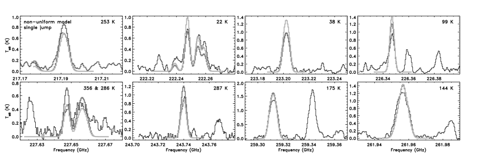
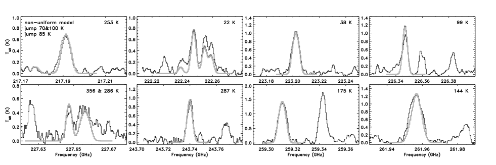
Figure 6: Selected emission lines for CH₃OCH₃, $\varv=0$, over-plotted with the best-fit non-uniform LIME model with a single jump of the CH₃OCH₃ abundance at 70 or 100 K (see Table 3). The observed spectrum is displayed in black, the model for CH₃OCH₃, $\varv=0$, with an abundance jump at 70 K in light grey and at 100 K in dark grey. The value of $E_{\rm u}$ for each transition is given in the upper right corner of each panel.

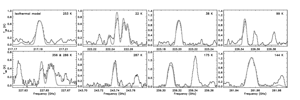
Figure 7: Same as Fig. 8, but with two jumps of the CH₃OCH₃ abundance at 70 and 100 K (light grey) and a single jump of the abundance at 85 K (dark grey). The observed spectrum is displayed in black.

Figure 8: Same as Fig. 8, but with the isothermal myXCLASS model over-plotted in grey (see Table 2 for the properties of the two isothermal components).

We have used the density and temperature profile for the source G327.3-0.6 calculated by Rolffs et al. (2011) and modeled the dimethyl ether emission with the new radiative transfer tool LIME (Brinch & Hogerheijde, 2010). Rolffs et al. (2011) approximate the density and temperature profile of G327.3-0.6 with a spherical model based on the 870 $\mu$m dust radial profile observed with the Large APEX Bolometer Camera (LABOCA) in the ATLASGAL project (APEX Telescope Large Area Survey of the Galaxy, Schuller et al., 2009). In the model the source has a luminosity of 7$\times$10⁴ L_⊙, a temperature of 55 K at the photospheric radius (i.e., diffusion sets the temperature gradient in the inner region, and the balance between heating and cooling sets the temperature gradient in the outer region), and a density of 3.5$\times$10⁶ cm^-3. The photospheric radius is derived by computing the Planck and Rosseland opacities and weighting them with the Planck function (see Rolffs et al., 2011, for the details). The model assumes the gas is static, and has a turbulent line width, $FWHM$, of 4 km s^-1.

The dimethyl ether in the non-uniform density and temperature LIME models is assumed to be in LTE as for the isothermal myXCLASS models presented in Sect. 4.1. The dust opacity has not been taken into account in the LIME models, due to issues of its implementation into the code in combination with overlapping transitions, which for dimethyl nearly always is the case. For this reason we have chosen to use only low frequency dimethyl ether transitions (up to: 261956 MHz) for which the dust is optically thin (see Sect. 3.2) and thus does not affect the model results significantly. Another assumption is that CH₃OCH₃ evaporates above 70 K and that dimethyl ether’s precursor methanol evaporates at $\sim$100 K (see Sect. 1). The radii at which these temperatures occur are consistent with those found for the two components of the isothermal myXCLASS model described in Sect. 4.1.

To assess the accuracy of the models, we have performed a reduced $\chi^{2}$-analysis for the calculated emission for a set of 7 dimethyl ether transitions that span a range of temperatures and optical depths and are known to be free from emission line blends from our survey. In Table 3 we show the best reduced $\chi^{2}$ for the fits to the transitions shown in Figs. 8–8 for the non-uniform density and temperature models with the CH₃OCH₃ abundance jumping at a temperature ranging from 70 K up to 100 K. Results for the best-fit model with a jump at 70 K (light grey) and 100 K (dark grey) are also shown in Fig. 8, as well as the model with a jump at both 70 and 100 K (light grey) and a single jump at 85 K (dark grey) in Fig. 8. The reduced $\chi^{2}$ is calculated for a 10 km s^-1 wide window around the peak position except for the blended features (second and fifth panel), where the velocity range covered is 8 km s^-1 to avoid including emission from other species. Below the jump temperature the abundance is set to be negligible (1.0$\times$10^-15 w.r.t. H₂). For each jump temperature, we first tried to identify around which abundance the reduced $\chi^{2}$ was lowest and afterwards ran a set of 4–6 models with abundance steps of 1–2$\times$10^-8 to identify the best-fit abundance.

As can be seen in Fig. 8 the LIME model, where the abundance jump for CH₃OCH₃ occurs at 100 K, fits most emission lines very well, but seems to over-reproduce the transitions with the highest excitation energies. In contrast, the model where there is a single jump at 70 K, has the opposite problem, that the lower excitation transitions are over-produced, when those at high energies are well fit. When there are two abundance jumps at 70 and 100 K or one at an intermediate temperature of 85 K (see Fig. 8) this systematic mismatch of low or higher excitation transitions is not observed. The difference between the model with the abundance jump at 85 K and that with a jump at both 70 and 100 K is, however, negligible. Both models fit the observed line strength and width very well. It is only in the second panel for the 22 K lines that some deviation is seen for two weaker lines, which are slightly under-produced very likely due to unknown line blends.

Due to the similarities for the non-uniform density LIME models with a single or double abundance jump no conclusion about whether there are one or two jumps in the CH₃OCH₃ abundance, can be drawn. Finally, the models suggest that most dimethyl ether emission arises from a region with temperatures above 100 K, but that some emission seems to arise from a region with temperatures lower than 100 K.

Table 3: Results of the fits to a selected number of dimethyl ether transitions for both the non-uniform density and temperature LIME models as well as the isothermal myXCLASS models.

$T_{\rm jump}$	$\chi^{2}$	$x$(CH3OCH3)a	$\frac{\mathcal{N}_{\rm<100\leavevmode\nobreak\ K}{\rm(CH_{3}OCH_{3})}}{\mathcal{N}{\rm(CH_{3}OCH_{3})}}$
K		w.r.t. H2
Non-uniform density and temperature model
70	1.73	9$\times$10-8	0.41
80	1.31	1.1$\times$10-7	0.28
85	1.26	1.4$\times$10-7	0.21
90	1.33	1.4$\times$10-7	0.14
100	1.37	2.0$\times$10-7	0.00
70 & 100	1.32	3$\times$10-8 & 1.4$\times$10-7	0.05
Isothermal model
90	2.08	1.7$\times$10-7	0.14
80 & 100	1.34	5.9$\times$10-8 & 3.0$\times$10-7	0.08

^aThe abundance in the outermost part of the envelope, where temperatures are below 70 K, is assumed to be 1.0$\times$10^-15 with respect to H₂, i.e., negligible.

5 Discussion

5.1 Comparison of an isothermal source model with a non-uniform density and temperature model

In general, we can conclude that isothermal models for the dimethyl ether emission are in qualitative agreement with the models with a non-uniform source structure. This is demonstrated by the comparison of Figs. 8 and 8. There are small differences, i.e., the line wings are better fit with the isothermal model, whereas the line-centers are often better fit with the non-uniform source model. To compare the isothermal fit to the non-uniform spherical model, we have calculated a reduced $\chi^{2}$ for the myXCLASS models with one and two components of the same lines that are used in the LIME model. The isothermal model suggests two abundance jumps for CH₃OCH₃, as can be seen by the significantly lower value for $\chi^{2}$ for the two-component model (see Sect. 4.1). However, the non-uniform density and temperature models suggest that two separate abundance jumps are not needed. This suggests that dimethyl ether traces gas that has a temperature and density gradient. In a way our two-component isothermal model can be considered as a “simple” non-uniform density and temperature model. The non-uniform source model is therefore a useful tool for the interpretation of the emission of CH₃OCH₃ in the hot core of G327.3-0.6.

5.2 Implications for the formation mechanisms of CH₃OCH₃

The fact that CH₃OCH₃ is present in regions with a range of temperatures makes it difficult to separate the contribution of grain surface formation or gas phase formation and determine which is dominant. If we assume that dimethyl ether with excitation temperatures below 100 K is due to solid state formation, then it is possible to estimate the lower limit to the fraction of CH₃OCH₃ that is formed on icy grains. The reason we can only deduce lower limits is, that the dimethyl ether present at higher temperatures may also originate from solid state chemistry. A laboratory study by Collings et al. (2004) namely shows that many molecular species can be trapped in ices up to the H₂O evaporation temperature. For species with similar binding energies as CH₃OCH₃, about 50% remains trapped in the ice until the H₂O evaporates when it is co-deposited with water. This fraction is lower for layered ices, where the studied species was deposited on top of a water ice layer. Unfortunately, CH₃OCH₃ was not one of the species studied by Collings et al. (2004), but it is reasonable to assume that something similar would occur for dimethyl ether and that some fraction of the dimethyl ether gas at temperatures above 100 K is due to CH₃OCH₃ co-desorbing with H₂O.

In Table 3 we show the fractional contribution of the dimethyl ether containing gas that has a temperature between 70 and 100 K, $\frac{\mathcal{N}_{\rm<100\leavevmode\nobreak\ K}{\rm(CH_{3}OCH_{3})}}{\mathcal{N}{\rm(CH_{3}OCH_{3})}}$. $\mathcal{N}{\rm(CH_{3}OCH_{3})}$ is defined as the total number of dimethyl ether molecules in the model, and is derived by integrating over the radial density profile combined with the radial abundance dependence for dimethyl ether. $\mathcal{N}_{\rm<100\leavevmode\nobreak\ K}{\rm(CH_{3}OCH_{3})}$ is calculated in a similar way, but only by integrating over the part of the envelope that is below 100 K. If we consider the model with the abundance jump at 85 K, the fraction of dimethyl ether present in gas between 70 and 100 K is 21%. This would suggest that at least 21% is formed on icy grains. If we assume that the two-jump model is the most extreme case, since, as mentioned earlier in this section, the 100 K systematically under-reproduces all the lower excitation lines, then the models suggest that the lower limit to the grain surface contribution is 5% and conversely, this means that the upper limit to the gas phase contribution is 95%.

An alternative formation mechanism for low-temperature gas-phase dimethyl ether is that a small fraction of solid CH₃OH evaporates from the ices at low temperatures and gives rise to a small amount of CH₃OCH₃ that is formed in the cooler gas phase. For ¹³CH₃OH we have performed a similar analysis as described for dimethyl ether in this paper, i.e. we modeled its emission with both isothermal and a non-uniform density and temperature models. The best-fit abundances found for ¹³CH₃OH in non-uniform density and temperature models are 2($\pm$0.5)$\times$10^-11 and 4.5($\pm$0.5)$\times$10^-8, below and above 100 K, respectively. When we assume the ¹²C/¹³C ratio to be 53 the average found by Wilson & Rood (1994) for the 4 kpc molecular ring, the CH₃OH abundance below 100 K in G327.3-0.6 would be $\sim$1$\times$10^-9 and $\sim$2$\times$10^-6 above 100 K. This is consistent with models of both low and high-mass star-forming regions where the abundance of CH₃OH is on the order of 10^-10–10^-9 below 90–100 K (Schöier et al., 2006; Maret et al., 2005; Van der Tak et al., 2000). Since radiative dissociation experiments performed with CD₃OCD${}_{4}^{+}$ by Hamberg et al. (2010) only results in the formation of deuterated dimethyl ether in 7% of the reactions, and not all CH₃OH will react to form CH₃OCH${}_{4}^{+}$, we expect the CH₃OCH₃/CH₃OH ratio to be 0.07 at most, but probably much lower. The gas phase abundances of dimethyl ether formed at low temperatures is therefore likely not larger than 7$\times$10^-11. Additionally, CH₃OCH₃ itself may also desorb directly through non-thermal mechanisms. In theoretical models of grain-surface formation the solid state CH₃OCH₃/CH₃OH ratio is on the order of 10^-3–10^-4 (Garrod et al., 2008). The gas phase abundance of CH₃OCH₃ that could be due to non-thermal desorption is thus expected to be $\sim$10^-13, which is lower than the CH₃OCH₃ abundance that could be formed from non-thermally desorbed CH₃OH. Since abundances of $\sim$10^-8 for dimethyl ether are needed in the outer regions both in the isothermal case and for the non-uniform source models for the G327.3-0.6 high-mass star-forming region, the major contributor to cooler dimethyl ether gas cannot be direct non-thermally desorbed CH₃OCH₃ or gas phase formation through the non-thermal evaporation of CH₃OH. CH₃OCH₃ that desorbs thermally from icy grain surfaces is therefore most likely responsible for the CH₃OCH₃ emission below 100 K. Interestingly, the CH₃OCH₃/CH₃OH ratio above 100 K is in the 5–10% range for our non-spherical source models, which is close to the upper limit for the ratio expected from gas phase formation mechanism, underlining that although the data suggests that there is some grain-surface formation of dimethyl ether, the gas phase mechanism likely is dominant.

In summary, our non-uniform density and temperature LIME models of the emission of dimethyl ether, give qualitatively the same result as the isothermal myXCLASS model. They namely suggest that most emission of dimethyl ether arises from regions with temperatures of 100 K and higher, but that some fraction of dimethyl ether emission is present at lower temperatures. The most likely origin of this low temperature component is formation of dimethyl ether in the solid state.

6 Summary and conclusions

In this paper we have analyzed the rotational emission of CH₃OCH₃ in its ground state, $\varv=0$, and the torsionally excited states $\varv_{11}=1$ and $\varv_{15}=1$ for the source G327.3-0.6 observed with the Atacama Pathfinder EXperiment (APEX). The data have been modeled with an isothermal model as well as a radiative transfer model with a non-uniform spherical density and temperature structure. The main conclusions are:

• Many transitions from the ground state, $\varv=0$, of dimethyl ether are detected toward the high-mass star forming region G327.3-0.6. The emission can be very well described by a two-component isothermal model with two abundance jumps at 80 K and 100 K. Since dimethyl ether has both optically thin and moderately optically thick lines, it is a very suitable diagnostic for dense and fairly warm regions.

• A variety of lines from the $\varv_{11}=1$ and $\varv_{15}=1$ torsionally excited states of dimethyl ether are detected here for the first time. The emission can be well described by the same model as for the ground state. Due to the large line-strengths these states should also easily be detectable in other line-rich hot core sources, in particular with new upcoming interferometers such as the Atacama Large Millimeter Array (ALMA).

• Radiative transfer models with a non-uniform density and temperature structure show that the emission can be very well fit by an abundance jump in the dimethyl ether emission at either 85 K or by two abundance jumps at 70 and 100 K. In contrast two components are needed to accurately reproduce the emission with an isothermal model. We therefore conclude that the non-uniform density and temperature models suggest that dimethyl ether emission arises from an extended region with a significant density and temperature structure, but not necessarily has two abundance components. We estimate that the lower limit for the solid state vs. gas phase contribution is 5%. However, the large abundance ratio CH₃OCH₃/CH₃OH suggest that the gas phase formation mechanism is likely the major contributor.

The presented study shows the potential for these kind of surveys to constrain the chemical structure of high-mass protostellar hot cores. The study of CH₃O¹³CH₃ could potentially give additional clues to the formation of dimethyl ether. The ¹²C/¹³C ratio namely has the potential to distinguish between grain surface formation and gas phase formation of dimethyl ether (Charnley et al., 2004). This would make it possible to not just improve our understanding of the formation routes of dimethyl ether, but also address whether isotopologues in general can be used as important tracers of the chemistry in star-forming regions.

In addition, it would be interesting to perform similar analyses for a variety of complex organic species. This will make it possible to compare different molecular species with each other as well as to astrochemical models. Specifically, a strong correlation between the abundances of different complex organic species in large sample of star-forming regions, such as performed by Bisschop et al. (2007) may tell us whether two complex organic molecules likely are chemically related. In the longer term, high resolution interferometric measurements, in particular with ALMA, are key to understanding the origin of CH₃OCH₃ and other complex organics in star-forming regions. The higher spatial resolution will place better constraints on the physical structure of the source and will for example show whether the emission is clumpy or non-spherical. Also, such observations will show how the absolute abundances vary with temperature and thus reveal whether a given species comes off dust grains directly at its evaporation temperature - or perhaps is formed only at even higher temperatures in the gas-phase. From this it is possible to conclude what the relative importance of solid state and gas phase formation mechanisms are and for which key reactions laboratory investigations and quantum chemical calculations are most needed.

Appendix A Assignments of CH₃OCH₃, $\varv=0$, $\varv_{11}=1$, and $\varv_{15}=1$ for G327.3-0.6 in all observed frequency windows.

In this appendix we show the line parameters for all the unblended lines that have been detected for CH₃OCH₃, $\varv=0$ (Table LABEL:detfreqv0), $\varv_{11}=1$ (Table LABEL:detfreqv11), and $\varv_{15}=1$ (Table LABEL:detfreqv15). For questions about the full line-list please contact the authors. For all transitions frequencies, quantum numbers and the energies of the upper state ($E_{\rm u}$) are given as well as the measured integrated line intensities ($\int T_{\rm MB}dv$) and model line-intensities from the isothermal myXCLASS model for the dimethyl ether emission ($I_{\rm model}$). Most features are actually composed of a set of multiple transitions, and we therefore refer to Endres et al. (2009) and Endres et al. (in prep.) for the values of $\mu^{2}S$ for the individual transitions.

Table 4: Detections of CH₃OCH₃, $\varv=0$ towards G327.3-0.6.

Frequency	Transition	$E_{\rm u}$	$\int T_{\rm MB}dv$	$I_{\rm model}$
(MHz)		(K)	(K km s-1)	(K km s-1)
213453.7	213,1,20,3/5 – 211,0,21,3/5	212.92	1.60	1.30
213457.7	213,1,20,1 – 211,0,21,1	212.92	2.40	2.19
213461.7	213,1,20,0 – 211,0,21,0	212.92	1.42	1.24
214470.7	2811,5,23,0/1/3/5 – 289,4,24,0/1/3/5	406.35	2.54	1.76
217176.9	369,4,32,0/1/3/5 – 367,3,33,0/1/3/5	638.63	0.18	0.20
217191.0	228,4,19,0/1/3/5 – 226,3,20,0/1/3/5	253.41	4.75	5.44
218491.3	236,3,21,0/1/3/5 – 234,2,22,0/1/3/5	263.83	3.45	3.86
220893.0	238,4,20,0/1/3/5 – 236,3,21,0/1/3/5	274.44	4.44	4.16
222032.9	214,2,20,1 – 212,1,21,1	213.35	2.37	2.24
222037.1	214,2,20,0 – 212,1,21,0	213.35	1.05	0.88
222238.9	46,3,2,3 – 35,2,1,3	21.76	1.29	1.20
222254.6	46,3,2,0 – 35,2,1,0	21.76	3.89	4.21
222259.2	47,3,1,1/3 – 35,2,1,1/3	21.76	2.87	2.84
222325.4	256,3,23,0/1/3/5 – 249,4,20,0/1/3/5	308.17	1.19	0.75
222414.4	46,3,2,3 – 34,2,2,3	21.76	0.98	0.94
222426.7	47,3,1,5 – 34,2,2,5	21.76	1.45	1.10
223201.7	84,2,7,0/1/3/5 – 73,1,6,0/1/3/5	38.31	9.20	9.67
223408.8	265,2,24,0/1/3/5 – 263,1,25,0/1/3/5	330.39	2.61	2.54
225203.6	248,4,21,0/1/3/5 – 246,3,22,0/1/3/5	296.37	4.38	4.54
225599.0	122,1,12,0/1/3/5 – 111,0,11,0/1/3/5	69.79	8.49	9.83
226347.1	143,1,13,0/1/3/5 – 134,2,12,0/1/3/5	98.86	6.34	6.81
226491.3	223,1,21,3/5 – 221,0,22,3/5	232.58	0.68	0.71
226495.5	223,1,21,1 – 221,0,22,1	232.58	1.90	2.11
226499.7	223,1,21,0 – 221,0,22,0	232.58	0.91	0.82
227647.3	2611,5,21,0/1/3/5 – 269,4,22,0/1/3/5	355.77	2.12	2.67
227655.8	246,3,22,0/1/3/5 – 244,2,23,0/1/3/5	285.56	4.90	4.67
228423.2	266,3,24,0/1/3/5 – 259,4,21,0/1/3/5	331.65	1.16	0.77
230141.1	258,4,22,0/1/3/5 – 256,3,23,0/1/3/5	319.21	4.74	3.40
230234.1	175,2,15,0/1/3/5 – 166,3,14,0/1/3/5	147.65	7.16	5.80
232383.1	379,4,33,0/1/3/5 – 377,3,34,0/1/3/5	673.01	0.40	0.27
233189.1	224,2,21,3/5 – 222,1,22,3/5	232.92	1.64	1.47
233193.4	224,2,21,1 – 222,1,22,1	232.92	1.80	2.11
233197.6	224,2,21,0 – 222,1,22,0	232.92	1.62	1.39
233632.1	2511,5,20,0/1/3/5 – 259,4,21,0/1/3/5	331.90	3.10	3.87
235714.2	268,4,23,0/1/3/5 – 266,3,24,0/1/3/5	342.96	3.46	3.69
237048.2	75,2,5,0/1/3/5 – 62,1,6,0/1/3/5	31.26	9.97	9.17
237620.4	94,2,8,0/1/3/5 – 83,1,7,0/1/3/5	46.46	10.59	9.44
238956.4	327,3,29,0/1/3/5 – 325,2,30,0/1/3/5	501.84	1.71	0.81
239322.0	233,1,22,3/5 – 231,0,23,3/5	253.09	1.08	1.30
239326.4	233,1,22,1 – 231,0,23,1	253.09	1.92	2.18
239330.8	233,1,22,0 – 231,0,23,0	253.09	0.95	1.01
240978.3	56,3,3,3 – 45,2,2,3	26.31	2.71	2.19
240983.9	56,3,3,1/5 – 45,2,2,1/5	26.31	8.19	6.96
240990.0	56,3,3,0 – 45,2,2,0	26.31	4.02	3.33
241507.9	56,3,3,1 – 44,2,3,1	26.31	1.36	0.73
241637.7	217,3,18,0/1/3/5 – 208,4,17,0/1/3/5	225.70	4.96	3.69
243739.6	2311,5,18,0/1/3/5 – 239,4,19,0/1/3/5	286.98	5.58	5.69
243796.0	3213,6,26,0/1/3/5 – 3114,7,25,0/1/3/5	532.72	0.77	0.21
244508.3	234,2,22,1 – 232,1,23,1	253.35	2.61	2.01
247771.7	2211,5,17,0/1/3/5 – 229,4,18,0/1/3/5	265.92	4.34	5.67
248754.8	288,4,25,0/1/3/5 – 286,3,26,0/1/3/5	393.15	3.15	2.73
251142.0	2111,5,16,0/1/3/5 – 219,4,17,0/1/3/5	245.80	8.21	7.46
251583.2	104,2,9,0/1/3/5 – 93,1,8,0/1/3/5	55.51	12.07	12.00
251971.0	243,1,23,1 – 241,0,24,1	274.44	2.23	1.81
251975.6	243,1,23,0 – 241,0,24,0	274.44	1.31	0.79
252277.7	1520/21,10,5/6,0/1/3/5 – 1618/19,9,7/8,0/1/3/5	249.69	2.12	1.25
255942.3	244,2,23,3/5 – 242,1,24,3/5	274.64	1.92	1.25
256136.7	1911,5,14,0/1/3/5 – 199,4,15,0/1/3/5	208.32	10.75	9.53
256193.5	298,4,26,0/1/3/5 – 296,3,27,0/1/3/5	419.59	2.48	2.12
259311.4	1711,5,12,0/1/3/5 – 179,4,13,0/1/3/5	174.54	12.38	11.21
259689.8	2310,5,19,0/1/3/5 – 238,4,20,0/1/3/5	286.90	6.17	5.58
259731.7	2110,5,17,0/1/3/5 – 218,4,18,0/1/3/5	245.76	5.48	6.88
260616.7	2510,5,21,0/1/3/5 – 258,4,22,0/1/3/5	331.72	5.00	4.34
260727.2	1810,5,14,0/1/3/5 – 188,4,15,0/1/3/5	190.97	8.82	10.66
260757.6	67,3,3,0/1/3/5 – 54,2,4,0/1/3/5	31.77	12.58	12.69
261563.1	1610,5,12,0/1/3/5 – 168,4,13,0/1/3/5	159.03	13.22	12.34
261584.6	2610,5,22,0/1/3/5 – 268,4,23,0/1/3/5	355.51	4.91	4.50
261955.9	1510,5,11,0/1/3/5 – 158,4,12,0/1/3/5	144.44	12.16	11.55
262312.4	1410,5,10,0/1/3/5 – 148,4,11,0/1/3/5	130.76	16.18	14.27
262384.5	1310,5,9,1 – 139,4,9,1	118.00	2.24	1.84
262392.7	1311,5,8,0/1/3/5 – 139,4,9,0/1/3/5	118.00	12.90	12.93
262754.8	1210,5,8,3 – 129,4,8,3	106.16	1.21	1.08
262884.3	1210,5,8,3 – 128,4,9,3	106.16	1.91	1.87
262889.8	1210,5,8,1/5 – 128,4,9,1/5	106.16	8.31	8.19
262897.1	1210/11,5,7/8,0/1/3 – 128,4,9,0/1/3	106.16	9.36	7.73
262964.4	2710,5,23,0/1/3/5 – 278,4,24,0/1/3/5	380.23	4.36	3.21
263035.3	1110,5,7,3 – 119,4,7,3	95.23	1.40	1.10
263043.4	1110/11,5,6/7,1/5 – 119,4,7,1/5	95.23	7.21	6.47
263049.9	1111,5,6,0/1/3 – 119,4,7,0/1/3	95.23	7.87	8.63
263102.1	1110,5,7,3 – 118,4,8,3	95.23	2.57	2.07
263107.7	1110,5,7,1/5 – 118,4,8,1/5	95.23	6.86	6.30
263241.1	1010,5,6,3 – 109,4,6,3	85.21	1.17	0.74
263250.4	1010/11,5,5/6,1/5 – 109,4,6,1/5	85.21	4.97	4.68
263256.8	1011,5,5,0/1/3 – 109,4,6,0/1/3	85.21	7.75	8.29
263413.5	910,5,5,1/3/5 – 98,4,6,1/3/5	76.11	7.28	7.37
263421.6	910/11,5,4/5,0/1 – 98,4,6,0/1	76.11	5.88	5.67
263582.9	710/11,5,2/3,0/1/3/5 – 78/9,4,3/4,0/1/3/5	60.63	18.66	17.25
263658.0	510/11,5,0/1,0/1/3/5 – 58/9,4,1/2,0/1/3/5	48.80	8.61	11.15
264211.2	308,4,27,0/1/3/5 – 306,3,28,0/1/3/5	446.91	3.33	2.30
264809.6	2810,5,24,0/1/3/5 – 288,4,25,0/1/3/5	405.86	4.17	3.26
264927.1	399,4,35,0/1/3/5 – 397,3,36,0/1/3/5	744.36	0.33	0.16
265152.2	114,2,10,0/1/3/5 – 103,1,9,0/1/3/5	65.45	10.80	11.44
267169.4	2910,5,25,0/1/3/5 – 298,4,26,0/1/3/5	432.41	3.81	2.38
267477.7	254,2,24,3/5 – 252,1,25,3/5	296.78	1.05	0.87
267482.5	254,2,24,1 – 252,1,25,1	296.78	1.47	1.63
271288.8	1420/21,10,4/5,0/1/3/5 – 1518/19,9,6/7,0/1/3/5	236.04	0.98	1.39
272599.1	1722/23,11,6/7,0/1/3/5 – 1820/21,10,8/9,0/1/3/5	309.18	1.96	1.11
272774.5	318,4,28,0/1/3/5 – 316,3,29,0/1/3/5	475.12	2.56	1.60
273107.3	163,1,15,0/1/3/5 – 154,2,14,0/1/3/5	127.20	8.05	9.80
273384.5	269,4,22,0/1/3/5 – 2510,5,21,0/1/3/5	344.84	1.86	1.64
273597.9	3110,5,27,0/1/3/5 – 318,4,28,0/1/3/5	488.25	1.57	1.67
273848.9	2024/25,12,8/9,0/1/3/5 – 2122/23,11,10/11,0/1/3/5	393.30	0.87	0.61
275381.8	152,1,15,0/1/3/5 – 141,0,14,0/1/3/5	106.39	11.61	13.25
276796.0	263,1,25,3/5 – 261,0,26,3/5	319.67	1.11	0.76
277039.6	3110,5,27,0/1/3/5 – 3013,6,24,0/1/3/5	488.25	1.51	0.48
277533.0	3313,6,27,0/1/3/5 – 3311,5,28,0/1/3/5	563.01	2.04	1.17
277647.4	76,3,5,0/1/3/5 – 65,2,4,0/1/3/5	38.15	17.58	15.53
278406.6	124,2,11,0/1/3/5 – 113,1,10,0/1/3/5	76.28	15.82	14.05
279097.5	264,2,25,0 – 262,1,26,0	319.78	1.75	0.94
280167.4	305,2,28,0/1/3/5 – 303,1,29,0/1/3/5	433.71	3.73	1.80
280187.9	77,3,4,0/1/3/5 – 64,2,5,0/1/3/5	38.15	24.89	17.50
280938.2	48/9,4,0/1,0/1/3/5 – 36/7,3,0/1,0/1/3/5	31.60	28.79	25.01
281844.0	328,4,29,0/1/3/5 – 326,3,30,0/1/3/5	504.21	2.53	1.56
283946.0	195,2,17,0/1/3/5 – 186,3,16,0/1/3/5	182.11	9.31	8.30
284234.6	3213,6,26,0/1/3/5 – 3211,5,27,0/1/3/5	532.72	1.94	1.28
286159.5	357,3,32,0/1/3/5 – 355,2,33,0/1/3/5	595.37	1.29	0.76
288174.1	308,4,27,0/1/3/5 – 2911,5,24,0/1/3/5	446.91	2.14	0.76
288903.6	1018/19,9,1/2,0/1/3/5 – 1116/17,8,3/4,0/1/3/5	163.87	1.95	0.98
289871.6	117,3,8,3/5 – 111,0,11,3/5	72.87	1.07	0.41
289877.9	117,3,8,1 – 111,0,11,1	72.87	0.78	0.66
289884.2	117,3,8,0 – 111,0,11,0	72.87	0.37	0.40
290758.5	274,2,26,1 – 272,1,27,1	343.63	1.37	1.26
290763.6	274,2,26,0 – 272,1,27,0	343.63	1.05	0.57
291442.7	134,2,12,0/1/3/5 – 123,1,11,0/1/3/5	88.00	12.92	13.33
292412.4	162,1,16,0/1/3/5 – 151,0,15,0/1/3/5	120.30	13.71	15.98
293628.2	315,2,29,0/1/3/5 – 313,1,30,0/1/3/5	461.62	3.33	1.98
293994.8	3510,5,31,0/1/3/5 – 358,4,32,0/1/3/5	610.85	0.57	0.61
294046.6	2226/27,13,9/10,0/1/3/5 – 2324/25,12,11/12,0/1/3/5	467.46	0.85	0.39
295337.5	86,3,6,0/1/3/5 – 75,2,5,0/1/3/5	45.44	18.55	19.55
295374.4	3210,5,28,0/1/3/5 – 3113,6,25,0/1/3/5	517.54	0.81	0.46
295513.6	3013,6,24,0/1/3/5 – 3011,5,25,0/1/3/5	474.96	3.71	2.30
295799.9	173,1,16,0/1/3/5 – 164,2,15,0/1/3/5	142.65	10.43	12.56
298159.2	237,3,20,0/1/3/5 – 228,4,19,0/1/3/5	267.72	6.67	5.04
299139.7	127,3,9,0 – 121,0,12,0	83.87	0.46	0.22
300704.8	3610,5,32,0/1/3/5 – 368,4,33,0/1/3/5	643.75	0.99	0.61
303705.2	3111,5,26,0/1/3/5 – 3012,6,25,0/1/3/5	489.44	1.29	0.79
304372.3	144,2,13,0/1/3/5 – 133,1,12,0/1/3/5	100.61	15.38	15.84
306823.8	325,2,30,0/1/3/5 – 323,1,31,0/1/3/5	490.37	2.39	1.32
307184.7	2713/22,6,21/41,0/1/3/5 – 2711/24,5,22/39,0/1/3/5	395.32	4.65	4.92
308035.9	3710,5,33,0/1/3/5 – 378,4,34,0/1/3/5	677.54	1.11	0.40
309606.2	172,1,17,0/1/3/5 – 161,0,16,0/1/3/5	135.07	10.93	16.09
309896.1	2613,6,20,0/1/3/5 – 2611,5,21,0/1/3/5	370.64	5.55	4.92
310300.3	137,3,10,3/5 – 131,0,13,3/5	95.81	1.07	0.59
310306.5	137,3,10,1 – 131,0,13,1	95.81	1.53	0.87
310784.1	205,2,18,0/1/3/5 – 196,3,17,0/1/3/5	200.68	8.86	8.57
312763.5	2912,6,24,0/1/3/5 – 2910,5,25,0/1/3/5	447.42	3.68	3.15
313238.1	293,1,28,1 – 291,0,29,1	393.84	2.22	1.11
337421.1	215,2,19,0/1/3/5 – 206,3,18,0/1/3/5	220.14	10.71	11.12
337731.6	78/9,4,3/4,0/1/3 – 67,3,3,0/1/3	47.98	12.06	14.41
337770.6	78,4,4,3 – 66,3,4,3	47.98	5.40	4.67
337778.8	78/9,4,3/4,1/5 – 66,3,4,1/5	47.98	12.39	13.84
338924.9	157,3,12,0 – 151,0,15,0	122.54	0.82	0.53
339491.5	193,1,18,0/1/3/5 – 184,2,17,0/1/3/5	176.10	8.59	16.08
340611.8	107,3,7,0/1/3/5 – 94,2,8,0/1/3/5	62.81	18.05	20.10
342608.0	191,0,19,0/1/3/5 – 182,1,18,0/1/3/5	167.14	13.11	19.89
349805.4	115,2,9,0/1/3/5 – 102,1,10,0/1/3/5	66.48	13.90	13.79
357460.0	184,2,17,0/1/3/5 – 173,1,16,0/1/3/5	159.81	14.20	19.20
358452.2	510/11,5,0/1,0/1/3/5 – 48/9,4,0/1,0/1/3/5	48.80	41.06	37.90
359383.8	126,3,10,0/1/3/5 – 115,2,9,0/1/3/5	83.73	24.95	24.15
360584.6	201,0,20,0/1/3/5 – 192,1,19,0/1/3/5	184.48	16.99	19.59
626982.8	351/2,0,35,0/1/3/5 – 341/2,1,34,0/1/3/5	546.61	27.69	29.55
628663.9	1016/17,8,2/3,0/1/3/5 – 914/15,7,2/3,0/1/3/5	140.00	57.66	80.92
628768.9	345,2,32,0/1/3/5 – 336,3,31,0/1/3/5	550.38	12.92	9.49
630494.3	288,4,25,0/1/3/5 – 277,3,24,0/1/3/5	393.15	11.36	20.12
632057.9	166,3,14,0/1/3/5 – 151,0,15,0/1/3/5	136.60	9.27	9.64
632281.8	357,3,32,0/1/3/5 – 348,4,31,0/1/3/5	595.37	6.51	6.74
636469.7	2010,5,16,0/1/3/5 – 199,4,15,0/1/3/5	226.58	34.17	44.47
637836.2	346,3,32,0/1/3/5 – 335,2,31,0/1/3/5	550.56	11.78	12.85
638541.0	298,4,26,0/1/3/5 – 287,3,25,0/1/3/5	419.59	13.55	13.74
638587.5	353,1,34,0/1/3/5 – 344,2,33,0/1/3/5	565.07	10.42	13.95
638957.7	354,2,34,0/1/3/5 – 343,1,33,0/1/3/5	565.08	11.15	11.96
641363.2	2011,5,15,0/1/3/5 – 198,4,16,0/1/3/5	226.60	26.65	40.84
643644.6	1712/13,6,11/12,0/1/3/5 – 1611,5,11,0/1/3/5	189.92	37.00	50.81
644668.1	361/2,0,36,0/1/3/5 – 351/2,1,35,0/1/3/5	577.55	20.11	25.03
645928.6	1414/15,7,7/8,0/1/3/5 – 1312/13,6,7/8,0/1/3/5	164.44	49.84	75.50
646090.4	229,4,18,0/1/3/5 – 216,3,19,0/1/3/5	254.03	20.23	30.99
646763.2	308,4,27,0/1/3/5 – 297,3,26,0/1/3/5	446.91	14.57	16.98
647198.6	217,3,18,0/1/3/5 – 204,2,19,0/1/3/5	225.70	20.69	24.41
647447.9	355,2,33,0/1/3/5 – 346,3,32,0/1/3/5	581.64	10.73	10.42
647614.2	1116/17,8,3/4,0/1/3/5 – 1014/15,7,3/4,0/1/3/5	150.01	40.19	82.64
653245.5	2110,5,17,0/1/3/5 – 209,4,16,0/1/3/5	245.76	25.02	39.18
654400.7	356,3,33,0/1/3/5 – 345,2,32,0/1/3/5	581.78	13.01	8.44
656308.2	363,1,35,0/1/3/5 – 354,2,34,0/1/3/5	596.58	7.26	9.56
656578.2	364,2,35,0/1/3/5 – 353,1,34,0/1/3/5	596.58	13.57	11.19
660459.7	2111,5,16,0/1/3/5 – 208,4,17,0/1/3/5	245.80	29.83	42.09
662323.0	1812/13,6,12/13,0/1/3/5 – 1711,5,12,0/1/3/5	206.33	35.74	54.82
662348.7	371/2,0,37,0/1/3/5 – 361/2,1,36,0/1/3/5	609.34	21.02	21.66
662413.9	1812/13,6,12/13,0/1/3/5 – 1710,5,13,0/1/3/5	206.33	37.21	48.02
664193.0	176,3,15,0/1/3/5 – 161,0,16,0/1/3/5	152.09	7.32	7.33
664346.3	328,4,29,0/1/3/5 – 317,3,28,0/1/3/5	504.21	11.21	13.16
664819.5	1514/15,7,8/9,0/1/3/5 – 1412/13,6,8/9,0/1/3/5	178.09	41.21	75.76
665894.4	365,2,34,0/1/3/5 – 356,3,33,0/1/3/5	613.74	8.20	7.08
668081.6	918/19,9,0/1,0/1/3/5 – 816/17,8,0/1,0/1/3/5	154.78	57.65	88.34
669407.7	2210,5,18,0/1/3/5 – 219,4,17,0/1/3/5	265.87	28.02	41.84
669682.4	399,4,35,0/1/3/5 – 3810,5,34,0/1/3/5	744.36	2.61	1.31
670814.3	3124/25,12,19/20,0/1/3/5 – 3122/23,11,20/21,0/1/3/5	653.53	11.68	7.16
671178.2	2924/25,12,17/18,0/1/3/5 – 2922/23,11,18/19,0/1/3/5	598.02	13.48	10.81
671198.8	366,3,34,0/1/3/5 – 355,2,33,0/1/3/5	613.85	15.66	8.92
671466.2	2724/25,12,15/16,0/1/3/5 – 2722/23,11,16/17,0/1/3/5	546.16	16.16	14.89
671689.0	2524/25,12,13/14,0/1/3/5 – 2522/23,11,14/15,0/1/3/5	497.93	21.21	20.62
671779.0	2424/25,12,12/13,0/1/3/5 – 2422/23,11,13/14,0/1/3/5	475.18	22.15	23.11
671856.4	2324/25,12,11/12,0/1/3/5 – 2322/23,11,12/13,0/1/3/5	453.35	20.88	25.42
672060.7	1924/25,12,7/8,0/1/3/5 – 1922/23,11,8/9,0/1/3/5	375.10	24.28	33.51
672090.4	1824/25,12,6/7,0/1/3/5 – 1822/23,11,7/8,0/1/3/5	357.81	25.83	34.48
672113.4	1724/25,12,5/6,0/1/3/5 – 1722/23,11,6/7,0/1/3/5	341.43	25.48	35.82
679792.0	2211,5,17,0/1/3/5 – 218,4,18,0/1/3/5	265.92	26.13	36.14
680024.2	381/2,0,38,0/1/3/5 – 371/2,1,37,0/1/3/5	641.98	20.48	17.64
680925.1	1912,6,14,0/1/3/5 – 1811,5,13,0/1/3/5	223.65	40.75	49.02
681091.0	1913,6,13,0/1/3/5 – 1810,5,14,0/1/3/5	223.65	42.16	53.23
683690.1	1614/15,7,9/10,0/1/3/5 – 1512/13,6,9/10,0/1/3/5	192.66	51.27	75.33
684154.8	375,2,35,0/1/3/5 – 366,3,34,0/1/3/5	646.68	10.35	7.29
684318.4	348,4,31,0/1/3/5 – 337,3,30,0/1/3/5	565.03	11.87	9.39
684840.6	2310,5,19,0/1/3/5 – 229,4,18,0/1/3/5	286.90	19.66	35.29
685339.0	227,3,19,0/1/3/5 – 214,2,20,0/1/3/5	246.24	14.33	18.02
691699.9	383,1,37,0/1/3/5 – 374,2,36,0/1/3/5	662.13	9.84	6.33
695424.5	358,4,32,0/1/3/5 – 347,3,31,0/1/3/5	596.74	6.65	6.46
697694.6	391/2,0,39,0/1/3/5 – 381/2,1,38,0/1/3/5	675.46	18.29	14.53
699453.7	2311,5,18,0/1/3/5 – 228,4,19,0/1/3/5	286.98	28.47	40.05
699720.5	2013,6,14,0/1/3/5 – 1910,5,15,0/1/3/5	241.89	33.38	46.34
701430.7	249,4,20,0/1/3/5 – 236,3,21,0/1/3/5	297.50	17.26	25.49
702536.5	1714/15,7,10/11,0/1/3/5 – 1612/13,6,10/11,0/1/3/5	208.15	33.23	74.93
704427.9	1416/17,8,6/7,0/1/3/5 – 1314/15,7,6/7,0/1/3/5	185.50	63.64	83.17
705856.3	168,4,13,0/1/3/5 – 153,1,14,0/1/3/5	146.48	9.56	6.27
705994.0	1118/19,9,2/3,0/1/3/5 – 1016/17,8,2/3,0/1/3/5	173.88	52.59	89.53
713083.1	2510,5,21,0/1/3/5 – 249,4,20,0/1/3/5	331.72	11.07	30.37
787947.6	2728/29,14,13/14,0/1/3/5 – 2726/27,13,14/15,0/1/3/5	619.00	6.56	10.96
788002.3	2628/29,14,12/13,0/1/3/5 – 2626/27,13,13/14,0/1/3/5	594.43	11.67	13.13
788048.5	2528/29,14,11/12,0/1/3/5 – 2526/27,13,12/13,0/1/3/5	570.78	15.47	15.68
788086.8	2428/29,14,10/11,0/1/3/5 – 2426/27,13,11/12,0/1/3/5	548.04	12.90	17.75
788118.2	2328/29,14,9/10,0/1/3/5 – 2326/27,13,10/11,0/1/3/5	526.21	13.15	18.71
788143.1	2228/29,14,8/9,0/1/3/5 – 2226/27,13,9/10,0/1/3/5	505.28	12.18	19.20
788162.2	2128/29,14,7/8,0/1/3/5 – 2126/27,13,8/9,0/1/3/5	485.27	18.32	26.32
789633.3	2512,6,20,0/1/3/5 – 2411,5,19,0/1/3/5	346.86	23.60	36.86
792378.1	2513,6,19,0/1/3/5 – 2410,5,20,0/1/3/5	346.88	36.72	41.90
796239.4	2214/15,7,15/16,0/1/3/5 – 2113,6,15,0/1/3/5	299.26	29.22	52.92
796271.1	2214/15,7,15/16,0/1/3/5 – 2112,6,16,0/1/3/5	299.26	24.85	47.50
798478.6	279,4,23,0/1/3/5 – 266,3,24,0/1/3/5	369.97	22.50	19.76
798877.2	1916/17,8,11/12,0/1/3/5 – 1814/15,7,11/12,0/1/3/5	262.88	42.49	77.54
800697.2	1618/19,9,7/8,0/1/3/5 – 1516/17,8,7/8,0/1/3/5	237.58	54.51	86.60
802211.8	1320/21,10,3/4,0/1/3/5 – 1218/19,9,3/4,0/1/3/5	223.30	45.12	95.30
804995.2	3610,5,32,0/1/3/5 – 359,4,31,0/1/3/5	643.75	8.37	5.22
806877.8	2612,6,21,0/1/3/5 – 2511,5,20,0/1/3/5	370.62	29.87	38.87
807366.8	2811,5,23,0/1/3/5 – 278,4,24,0/1/3/5	406.35	23.48	22.21
809302.3	257,3,22,0/1/3/5 – 244,2,23,0/1/3/5	313.48	20.60	13.20
810927.9	2613,6,20,0/1/3/5 – 2510,5,21,0/1/3/5	370.64	24.02	33.76
814832.8	2314/15,7,16/17,0/1/3/5 – 2213,6,16,0/1/3/5	320.23	37.26	45.37
814887.8	2314/15,7,16/17,0/1/3/5 – 2212,6,17,0/1/3/5	320.23	42.92	50.98
817709.4	2016/17,8,12/13,0/1/3/5 – 1914/15,7,12/13,0/1/3/5	281.09	56.78	74.67
829561.2	2713,6,21,0/1/3/5 – 2610,5,22,0/1/3/5	395.32	17.67	33.88

Table 5: Detections of CH₃OCH₃, $\varv_{11}=1$, transitions found to be free of emission from other species towards G327.3-0.6.

Frequency	Transition	$E_{\rm u}$	$\int T_{\rm MB}dv$	$I_{\rm model}$
(MHz)		(K)	(K km s-1)	(K km s-1)
225226.4	121,12,0 – 110,11,0	355.67	1.15	0.68
225245.0	121,12,3/5 – 110,11,3/5	355.65	1.02	0.69
241538.1	131,13,3/5 – 120,12,3/5	366.97	0.83	0.50
250263.7	140,14,5/3/1/0 – 131,13,5/3/1/0	378.98	3.85	2.20
252067.7	215,16,1 – 214,17,1	531.33	1.36	0.34
254754.5	205,15,1 – 204,16,1	512.19	0.85	0.40
255091.1	182,16,1 – 173,15,1	450.02	0.54	0.28
256924.9	195,14,1 – 194,15,1	493.96	0.90	0.44
258658.3	185,13,1 – 184,14,1	476.65	0.53	0.46
259390.2	63,3,1 – 52,3,1	317.77	0.87	0.35
259930.5	175,12,0 – 174,13,0	460.26	0.48	0.32
260577.5	205,16,1 – 204,17,1	512.17	0.45	0.40
261101.2	165,12,1 – 164,12,1	444.81	1.33	0.46
261929.1	155,11,1 – 154,11,1	430.25	0.63	0.46
261946.7	155,10,5 – 154,11,5	430.25	0.25	0.22
262098.5	165,12,0 – 164,13,0	444.80	0.68	0.40
262118.9	165,11,1 – 164,13,1	444.80	0.70	0.43
262233.2	165,12,5 – 164,13,5	444.81	0.33	0.22
262559.2	145,10,1 – 144,10,1	416.61	0.39	0.56
262853.3	145,9,1 – 144,11,1	416.60	1.93	0.56
263030.2	135,9,1 – 134,9,1	403.89	0.78	0.62
263172.1	135,8,1 – 134,10,1	403.88	0.73	0.57
263376.6	125,8,1 – 124,9,1	392.08	1.11	0.74
263867.9	105,5,1 – 104,6,1	371.17	1.13	0.72
263887.9	95,4,0 – 94,5,0	362.09	1.03	0.47
263900.2	95,5,0 – 94,6,0	362.10	0.39	0.25
264126.5	75,3,1 – 74,4,1	346.68	1.04	0.87
265066.9	112,10,1 – 101,9,1	351.33	1.19	0.89
271861.6	161,15,1 – 152,14,1	412.91	1.14	0.77
274852.3	151,15,0 – 140,14,0	392.19	0.93	0.68
274863.3	151,15,3/5 – 140,14,3/5	392.17	0.84	0.66
278357.5	122,11,3/5 – 111,10,3/5	362.14	1.87	0.59
287373.8	160,16,0/1/5/3 – 151,15,0/1/5/3	405.98	4.04	2.91
291296.6	132,12,0 – 121,11,0	373.84	0.82	0.42
291336.9	132,12,1 – 121,11,1	373.83	2.03	1.07
294544.9	171,16,1 – 162,15,1	428.33	0.72	0.94
294554.0	171,16,0 – 162,15,0	428.33	1.24	0.59
295247.3	83,6,1 – 72,5,1	331.40	0.77	0.93
295387.2	83,6,5 – 72,5,5	331.41	0.38	0.42
299810.4	83,5,1 – 72,6,1	331.42	1.03	0.98
304282.9	142,13,3/5 – 131,12,3/5	386.40	1.06	0.76
335248.7	212,19,5/3 – 203,18,5/3	505.59	0.37	0.28
335264.9	191,18,0 – 182,17,0	461.56	0.93	0.55
337758.6	74,4,0 – 63,3,0	333.99	1.34	1.18
340217.2	103,7,0 – 92,8,0	348.73	0.39	0.47
340319.9	103,7,1 – 92,8,1	348.72	1.83	1.27
341816.2	190,19,0/1/5/3 – 181,18,0/1/5/3	452.80	6.70	5.20
343478.9	172,16,0 – 161,15,0	429.39	0.93	0.66
343527.6	172,16,3/5 – 161,15,3/5	429.39	0.45	0.66
343633.1	191,19,0/1/3/5 – 180,18,0/1/3/5	452.84	4.74	4.33
344457.2	113,9,1 – 102,8,1	358.68	2.10	1.44
356510.4	84,5,0 – 73,4,0	341.25	1.44	1.30
356697.2	84,4,1 – 73,4,1	341.25	3.13	1.91
357143.8	182,17,1 – 171,16,1	445.46	1.70	1.71
359234.8	201,19,0/1/5/3 – 192,18,0/1/5/3	479.65	2.52	2.42
359431.3	123,10,5 – 112,9,5	369.59	0.76	0.48
361376.5	113,8,0 – 102,9,0	358.77	1.48	1.00
627228.3	137,7/6,5 – 126,6/7,5	437.66	3.01	2.78
627265.6	137,6,1 – 126,6,1	437.65	8.88	5.51
629100.8	108,3,1 – 97,3,1	426.09	2.64	6.50
629181.5	108,2/3,0 – 97,3/2,0	426.09	3.92	6.44
629240.9	108,3,3 – 97,3,3	426.11	2.20	1.75
643489.3	176,12,1 – 165,12,1	475.69	8.49	4.82
646021.1	147,8,1 – 136,8,1	450.36	6.78	5.18
646058.2	147,8/7,0 – 136,7/8,0	450.36	4.92	5.35
646120.9	147,7,1 – 136,7,1	450.36	4.34	5.40
648000.3	118,4,1 – 107,4,1	436.07	5.10	6.20
648028.4	118,3/4,5 – 107,4/3,5	436.08	4.04	3.28
648107.9	118,3,1 – 107,3,1	436.07	9.49	6.35
662135.1	186,13,1 – 175,13,1	492.06	6.12	4.29
662230.3	186,12,1 – 175,12,1	492.05	5.64	3.26
664862.9	157,9,1 – 146,9,1	463.99	7.29	4.83
664959.2	157,8,1 – 146,8,1	463.98	7.50	4.60
666999.2	128,4,1 – 117,4,1	446.97	10.95	6.34
668704.5	99,1/0,5 – 88,0/1,5	440.95	7.12	3.85
668725.0	99,1,1 – 88,1,1	440.94	12.45	7.04
683721.3	167,10/9,0 – 156,9/10,0	478.50	5.15	4.37
685782.6	138,6,1 – 127,6,1	458.76	6.64	5.55
685859.0	138,5/6,0 – 127,6/5,0	458.76	8.61	5.88
685883.7	138,5,1 – 127,5,1	458.77	7.80	5.98
685908.4	138,6,3 – 127,6,3	458.78	2.87	1.58
687609.8	109,2/1,5 – 98,1/2,5	450.03	3.66	3.50
687630.7	109,2,1 – 98,2,1	450.02	6.25	6.75
687718.6	109,1,1 – 98,1,1	450.03	7.59	6.72
687739.5	109,2/1,0 – 98,1/2,0	450.02	5.14	6.62
704684.9	148,6/7,5 – 137,7/6,5	471.48	5.77	2.64
704736.7	148,7/6,0 – 137,6/7,0	471.46	4.86	5.77
704759.5	148,6,1 – 137,6,1	471.47	5.57	5.90
706512.7	119,3/2,5 – 108,2/3,5	460.01	6.70	3.60
706534.0	119,3,1 – 108,3,1	460.00	9.51	6.96
706619.2	119,2,1 – 108,2,1	460.01	8.61	6.49
800977.5	169,8,1 – 158,8,1	523.53	5.32	4.87
801069.5	169,7/8,0 – 158,8/7,0	523.53	9.20	4.49
802803.8	1310,4,1 – 129,4,1	509.42	11.24	5.67
802845.4	1310,3,1 – 129,3,1	509.43	11.28	5.60
802910.7	1310,3/4,0 – 129,4/3,0	509.42	11.80	5.98
819842.5	179,9,1 – 168,9,1	538.96	8.43	4.44
821635.3	1410,4/5,5 – 139,5/4,5	522.13	1.89	2.84
821738.7	1410,4,1 – 139,4,1	522.14	13.15	5.52
821802.9	1410,5/4,0 – 139,4/5,0	522.13	10.80	5.63
823391.0	1111,1,1 – 1010,1,1	516.27	15.36	11.37

Table 6: Detections of CH₃OCH₃, $\varv_{15}=1$, found to be free of emission from other species towards G327.3-0.6.

Frequency	Transition	$E_{\rm u}$	$\int T_{\rm MB}dv$	$I_{\rm model}$
(MHz)		(K)	(K km s-1)	(K km s-1)
225482.3	121,12,0 – 110,11,0	416.36	0.54	0.18
225491.5	121,12,1 – 110,11,1	416.35	0.96	0.48
250026.9	140,14,5/3/1/0 – 131,13,5/3/1/0	439.66	2.58	1.37
260934.8	195,15,1 – 194,16,1	554.36	0.74	0.18
263123.2	135,8,1 – 134,9,1	464.45	0.27	0.28
263323.6	125,8,1 – 124,9,1	452.67	0.47	0.31
263389.0	125,7,1/3 – 124,8,1/3	452.65	1.25	0.41
263736.8	105,6,1 – 104,7,1	431.81	0.85	0.32
263780.7	105,5,1 – 104,6,1	431.80	1.18	0.32
263910.3	95,4,1 – 94,5,1	422.74	0.55	0.28
275036.2	151,15,0 – 140,14,0	452.87	1.12	0.54
275041.6	151,15,1 – 140,14,1	452.87	1.77	0.85
275047.0	151,15,3/5 – 140,14,3/5	452.86	0.88	0.50
280959.3	44,0/1,1 – 33,0/1,1	378.33	2.58	1.06
291989.8	161,16,0 – 150,15,0	466.75	0.41	0.45
291994.4	161,16,1 – 150,15,1	466.74	1.09	0.80
292026.2	132,12,0 – 121,11,0	434.44	0.45	0.31
292104.4	132,12,3/5 – 121,11,3/5	434.43	0.40	0.31
293172.6	171,16,1 – 162,15,1	488.83	1.04	0.41
299406.1	83,5,1 – 72,6,1	392.08	0.71	0.41
299831.1	54,1/2,1 – 43,1/2,1	382.87	1.44	1.23
305528.7	170,17,0/1/5/3 – 161,16,0/1/5/3	481.42	3.53	1.65
309117.5	171,17,1/3/5 – 160,16,1/3/5	481.49	3.19	1.63
337537.0	74,4,1 – 63,4,1	394.66	1.59	0.78
339584.9	103,7,0 – 92,8,0	409.36	0.53	0.39
341753.5	190,19,0/1 – 181,18,0/1	513.48	3.18	1.86
344404.1	172,16,1 – 161,15,1	489.95	2.07	0.76
356345.0	84,5,1 – 73,5,1	401.91	2.10	0.86
356374.3	84,4,1 – 73,4,1	401.90	1.62	0.75
356465.5	84,5,3 – 73,5,3	401.90	0.58	0.20
358158.2	201,19,5/1/3/0 – 192,18,5/1/3/0	540.12	2.80	1.47
358531.9	55,0,1 – 44,0,1	395.55	1.77	1.10
359724.0	200,20,0/1/5/3 – 191,19,0/1/5/3	530.79	4.57	2.54
361184.9	201,20,0/1/3/5 – 190,19,0/1/3/5	530.81	4.76	1.90
628753.2	108,2,1 – 97,2,1	486.70	5.91	3.58
647517.0	118,4,1 – 107,4,1	496.66	3.71	3.94
647590.4	118,3/4,0 – 107,4/3,0	496.65	4.93	3.86
666383.9	128,5,1 – 117,5,1	507.53	5.46	3.60
685244.6	138,6,1 – 127,6,1	519.32	4.89	3.87
685314.9	138,5/6,0 – 127,6/5,0	519.31	3.45	3.84
687251.5	109,1,1 – 98,1,1	510.62	7.40	4.84
706038.9	119,3,1 – 108,3,1	520.57	5.99	4.00