Transport across a junction of topological insulators and a superconductor

Abstract

We study transport across a line junction lying between two orthogonal topological insulator surfaces and a superconductor which can have either $s$-wave (spin-singlet) or $p$-wave (spin-triplet) pairing symmetry. We present a formalism for studying the effect of a general time-reversal invariant barrier at the junction and show that such a barrier can be completely described by three arbitrary parameters. We compute the charge and the spin conductance across such a junction and study their behaviors as a function of the bias voltage applied across the junction and the three parameters used to characterize the barrier. We find that the presence of topological insulators and a superconductor leads to both Dirac and Schrödinger-like features in charge and spin conductances. We discuss the effect of bound states on the superconducting side of the barrier on the conductance; in particular, we show that for triplet $p$-wave superconductors such a junction may be used to determine the spin state of its Cooper pairs. Our study reveals that there is a non-zero spin conductance for some particular spin states of the triplet Cooper pairs; this is an effect of the topological insulators which break the spin rotation symmetry. Finally, we find an unusual satellite peak (in addition to the usual zero bias peak) in the spin conductance for $p$-wave symmetry of the superconductor order parameter.

I Introduction

Recent theoretical zhang1 ; kane1 ; kane2 ; teo ; qi and experimental hasan1 ; exp2 ; exp1 ; hasan2 works have led to the discovery of a new class of materials called topological insulators (TI). In these materials the surface states have a gapless spectrum governed by a massless Dirac equation ti_rev ; these states contribute to charge transport at low temperatures. Such materials could be either in two or three spatial dimensions. A two-dimensional TI will host a one-dimensional gapless edge states while three-dimensional (3D) TI will host gapless states protected by time-reversal symmetry on its two-dimensional surface. The 3D TIs can be classified as strong or weak depending on whether the number of Dirac cones is odd or even, and this number is determined by a topological invariant. The odd number of Dirac cones on the surface of a strong TI is protected against time-reversal invariant (for instance, non-magnetic) perturbations for topological reasons kane2 ; zhang1 ; hasan1 . For materials such as $\rm Bi_{2}Te_{3}$ and ${\rm Bi_{2}Se_{3}}$, surfaces have been found which have a single Dirac cone near the $\Gamma$ point of the 2D surface Brillouin zone hasan1 ; exp2 ; hasan2 . Many interesting features of the surface Dirac electrons have been studied kane4 ; fu ; been1 ; tanaka1 ; mondal1 ; hasan2 ; burkov ; garate ; zyuzin ; das1 . Some of these studies involve interfaces created in a TI using proximate magnetic or superconducting materials or gate voltages kane4 ; been1 ; tanaka1 ; burkov ; garate ; das1 ; rein . Junctions of different surfaces of a TI (in some cases separated by a geometrical step or a magnetic domain wall) taka ; sen12 ; wickles ; biswas ; alos ; sitte ; zhang3 ; apalkov or of surfaces of a TI with normal metals or magnetic materials modak have also been studied. However, junctions of multiple TI surfaces with a superconductor have not been studied in detail so far; this is what we aim to do in this paper.

The problem of electron transmission across a junction of a normal metal (NM) and a superconductor (SC) has been extensively studied for many years btk ; kasta ; hayat ; tanaka95 ; kseng01 ; kseng02 ; kwon . It is well-known that the sub-gap transport in such junctions, for small barrier strengths, is governed by Andreev reflection while for large barrier strengths they reflect the sub-gap quasiparticle density of states (DOS)btk ; tanaka1 . Since the presence of localized quasiparticle edge states below the gap depends on the order parameter symmetry, such transport measurements, in the strong barrier limit, provide us with a tool for determining the pairing symmetry of the superconductor. In contrast, in the weak barrier limit, it was demonstrated that the conductance of a NM-SC junction can be more than the NM-NM conductance owing to Andreev reflection kasta . More recently, hybrid superconductor-semiconductor (${\rm Bi_{2}Te_{3}}$) devices has been successfully fabricated and conductance measurements in such systems has been carried out hayat . We note that these systems are somewhat akin to the junctions that we study in this work. However, the junction of a TI and a SC is expected to be more complex than its NM-SC counterpart. The reason for this complexity arises out of the fact that two-dimensional (2D) surface states of a TI display spin-momentum locking; hence scattering at a junction that changes the electron momentum couples different components of the electron spin. In contrast, the particle and hole are coupled to each other on the SC side. Hence a treatment of the transport between a TI and a SC necessarily requires us to use a four-component spinor formalism describing both spin and particle-hole degrees of freedom kseng01 ; kseng02 ; kwon .

In this work, we will analyze the transport properties for the system shown in Fig. 1. The system consists of two orthogonal TI surfaces, called TI-1 and TI-2. There is a two-dimensional SC surface which can be formed experimentally by depositing a 2D superconducting film on the surface of a 3D insulator. In what follows, we shall consider both singlet $s$-wave and triplet $p$-wave pairing symmetries for the superconducting film. The two TIs and the SC are separated by a line junction. We will consider a Dirac electron incident on the line junction from TI-1 with arbitrary angle of incidence and study its reflection (normal and Andreev) back to TI-1 and its transmission (normal and Andreev) into the TI-2 and the superconducting film. The main results that we obtain from such an analysis are the following. First, we develop appropriate boundary conditions for studying transmission across such a junction involving Dirac electrons in the TI and Schrödinger electrons in the superconductor. The general time-reversal invariant boundary condition is found to involve three parameters which can be interpreted as the strengths of three barriers close to the junction on the TI-1, TI-2 and SC sides. Second, using these boundary conditions, we compute the charge and spin conductances of such a junction as functions of the barrier strengths and the bias voltage and thus compare and contrast the properties of sub-gap transport in these junctions with their conventional counterparts. In particular, we find that for $\chi_{1}=\chi_{2}=0$, these junctions never reach the maximum charge conductance value $2G_{0}$ (where $G_{0}$ is an unit of conductance defined in Eq. (102)) found in conventional NM-SC junctions. Third, we find that, in contrast to all conventional NM-SC junctions, TI-SC junctions can be used to distinguish between the different spin states of the Cooper pair of a triplet $p$-wave superconductor. We show that such a property stems from the spin-momentum locking of the electrons on the TI surfaces. Fourth, we find that for a $p$-wave SC, the differential conductance has a zero-bias peak similar to the conventional NM-SC junctions; however for finite biases, the conductance both oscillates and decreases as the barrier strength increases which is to be contrasted with the monotonically decreasing nature of sub-gap conductance in conventional NM-SC junctions. Thus these junctions display both Dirac-like and Schrödinger-like characters. Finally, we find that there is a non-zero spin conductance for one particular component of the spin and two possible spin states of the triplet Cooper pairs. Further, we find that the differential spin conductance displays an unusual satellite peak away from zero bias and study the behavior of this peak with chemical potentials of the TI and SC surfaces and the barrier strengths of the junction.

The detailed plan of this paper is as follows. In Sec. II we write down the Hamiltonian for electrons on the topological insulator surfaces and the superconductors for both $s-$ and $p-$wave pairings and discuss their basic properties which will be useful in subsequent analysis. This is followed by Sec. III where we chart out the boundary conditions appropriate for transport through the junction. We utilize current conservation to discuss how the current gets converted from single quasiparticles (electrons or holes) near the junction to Cooper pairs deep inside the SC. Next, in Sec. IV, we use the boundary conditions to compute the transmission amplitudes of electrons from the TI-1 into the TI-2 and the SC and hence the charge conductance of the junction for arbitrary bias voltage, chemical potential difference, and barrier potential parameters. We discuss the obtained results in details in Sec. V. This is followed by Sec. VI where we study the spin transport through a $p$-wave SC with different pairing symmetries. Finally, in Sec. VII, we present a discussion of our results and some possible experiments to test our theory.

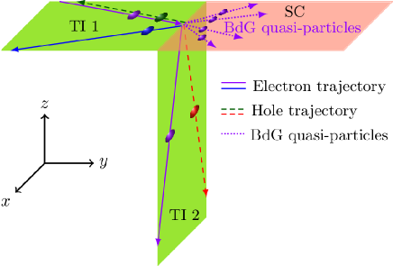
Figure 1: Schematic diagram of the proposed system with a line junction. Topological insulator surfaces 1 (lying in the $x-y$ plane with $y<0$) and 2 (lying in the $x-z$ plane with $z<0$) and a superconductor (lying in the $x-y$ plane with $y>0$) meet at a junction given by the line $y=z=0$. We indicate several processes which can be triggered by an electron incident from the TI-1 side: normal or Andreev reflection back to TI-1, normal of Andreev transmission to the TI-2 sides, and four possible BdG quasiparticle transmissions on the SC side (which eventually decay to zero and get converted to Cooper pairs).

II Hamiltonians

The Hamiltonian for the electrons on the surface of a TI is given by mondal1

$$H_{\hat{n}}=\int\frac{dk_{i}dk_{j}}{(2\pi)^{2}}\psi^{\dagger}_{\vec{k}}(\hbar v_{F}\hat{n}\cdot\vec{\sigma}\times\vec{k}-\mu_{\hat{n}}\mathds{1})\psi_{\vec{k}},$$ (1)

where $v_{F}$ is the Fermi velocity, the unit vector $\hat{n}$ points normal to the 2D surface, $k_{i},~{}k_{j}$ are momenta in the 2D plane, and $\psi_{\vec{k}}=(\psi_{\vec{k},\uparrow},~{}\psi_{\vec{k},\downarrow})^{T}$ is a two-component spinor. For TI-1, $\hat{n}=\hat{z}$ and $(i,j)=(x,y)$, while for TI-2, $\hat{n}=\hat{y}$ and $(i,j)=(x,z)$. The energy-momentum dispersion and the eigenstates on the TI-1 side are given by

$$E = -\mu_{1}\pm\hbar v_{1}\sqrt{k_{x}^{2}+k_{y}^{2}},$$

$$\psi_{1}^{\pm} = (1/\sqrt{2})~{}[1,~{}\mp ie^{i\theta_{1}}]^{T},$$

$$e^{i\theta_{1}} = (k_{x}+ik_{y})/\sqrt{k_{x}^{2}+k_{y}^{2}},$$ (2)

where $v_{1}$ is the Fermi velocity, and $\theta_{1}$ lies in the range $[0,\pi]$. In our calculations, we will consider the band which has the $+$ sign in the expression for the energy by choosing $\mu_{1}>0$ and working at energies $|E|<\mu_{1}$. On the TI-2 side, the dispersion and the eigenstates are given by

$$E = -\mu_{2}+\hbar v_{2}\sqrt{k_{x}^{2}+k_{z}^{2}},$$

$$\psi_{2}^{+} = (1/\sqrt{2})~{}[\sqrt{1+\cos{\theta_{2}}},~{}\sqrt{1-\cos{\theta_{2}}}]^{T},$$

$$e^{i\theta_{2}} = (k_{x}-ik_{z})/\sqrt{k_{x}^{2}+k_{z}^{2}}~{},$$ (3)

where $v_{2}$ is the Fermi velocity. To keep the discussion simple we choose $\mu_{1}=\mu_{2}=\mu_{TI}$. Also, our numerical results will be obtained for the case $v_{1}=v_{2}$ although we have retained the general form ($v_{2}\leq v_{1}$) in the important analytical expressions.

The wave functions on the SC side are described by a four-component Bogoliubov-de Gennes (BdG) spinor $\Psi$ whose upper two components correspond to particles and lower two components correspond to holes. Namely, $\Psi=[\psi_{\uparrow},~{}\psi_{\downarrow},~{}\psi^{*}_{\uparrow},~{}\psi^{*}_{\downarrow}~{}]^{T}$. (Note that many papers use the Nambu convention, with $\Psi=[\psi_{\uparrow},~{}\psi_{\downarrow},~{}-\psi^{*}_{\downarrow},~{}\psi^{*}_{\uparrow}~{}]^{T}$. In that convention, for example, factors of $i\sigma^{y}$ will not appear in Eq. (7)). In terms of the Pauli matrices $\sigma^{x,y,z}$ and $\tau^{x,y,z}$ which act on the spin and particle-hole components respectively, the Hamiltonian on the SC side can be written as

$$H_{3}~{}=~{}\int_{-\infty}^{\infty}dx\int_{0}^{\infty}dy~{}\Psi^{\dagger}(x,y)\Big{[} \Big{(}-\frac{\hbar^{2}\vec{\nabla}^{2}}{2m}-\mu_{SC}\Big{)}\tau^{z}$$

$$+~{}\Delta(x,y)\Big{]}\Psi(x,y),$$

where $\Delta(x,y)$ is called the pair potential. For our analysis of an $s$-wave SC (in which Cooper pairs form a spin singlet), we will take the pair potential to be of the form

$$\Delta(x,y) = \left(\begin{array}[]{cc}0&\Delta_{0}~{}i\sigma^{y}\\ -\Delta_{0}~{}i\sigma^{y}&0\end{array}\right).$$ (7)

$$\Delta(x,y) = \left(\begin{array}[]{cc}0&\Delta_{0}f(\vec{k})(\vec{d}\cdot\vec{\sigma})i\sigma^{y}\\ -\Delta_{0}f^{*}(\vec{k})(\vec{d}\cdot\vec{\sigma}^{*})i\sigma^{y}&0\end{array}\right)$$ (10)

(11)

where $\vec{d}$ is a unit vector with real components, and $f(\vec{k})$ is defined below. Physically, $\vec{d}$ governs the spin pairing of the Cooper pairs in the $p$-wave SC. For $\vec{d}=\hat{x}$, $\hat{y}$ and $\hat{z}$, a consideration of the matrix $(\vec{d}\cdot\vec{\sigma})i\sigma^{y}$ shows that the Cooper pairs are in the spin states $\uparrow\uparrow-\downarrow\downarrow$, $\uparrow\uparrow+\downarrow\downarrow$, and $\uparrow\downarrow+\downarrow\uparrow$, respectively. (In principle, $\vec{d}$ could depend on the momentum $\vec{k}$. However, in this work we are going to study systems with constant $\vec{d}$). In Eq. (11), $f(\vec{k})$ is a dimensionless linear function of $\vec{k}$ defined as

$$f(\vec{k}) \equiv -i(a_{x}\partial_{x}+a_{y}\partial_{y}),$$

$$f^{*}(\vec{k}) \equiv i(a^{*}_{x}\partial_{x}+a^{*}_{y}\partial_{y}),$$ (12)

where $a_{x},a_{y}$ are constants which may be complex. [In this paper we will consider wave functions in the SC which are of the form $e^{i(k_{x}x+k_{y}y)}$ where $k_{x}$ is real but $k_{y}$ may be complex. Hence there will not be any simple relation between $f(\vec{k})=\vec{a}\cdot\vec{k}$ and $f^{*}(\vec{k})=-\vec{a}^{*}\cdot\vec{k}$ in general]. In both Eqs. (7) and (11), $\Delta_{0}$ will be assumed to be a real parameter with dimensions of energy.

In a SC, the nature of the energy-momentum dispersion depends crucially on the symmetry of the superconducting pair potential. The dispersion is given by

$$E(\vec{k})=\pm\sqrt{\Big{[}\frac{\hbar^{2}(k_{x}^{2}+k_{y}^{2})}{2m}-\mu_{SC}\Big{]}^{2}+\Delta_{0}^{2}}$$ (13)

for an $s$-wave SC. For a $p$-wave SC, we can use the fact that $(\vec{d}\cdot\vec{\sigma})i\sigma^{y}(\vec{d}\cdot\vec{\sigma}^{*})i\sigma^{y}=\mathds{1}$ to show that

$$E=\pm\sqrt{\Big{[}\frac{\hbar^{2}(k_{x}^{2}+k_{y}^{2})}{2m}-\mu_{SC}\Big{]}^{2}+\Delta_{0}^{2}~{}(\vec{a}\cdot\vec{k})(\vec{a}^{*}\cdot\vec{k})}.$$ (14)

The important difference to note between the dispersions for these two kinds of pair potentials is that the superconducting gap is always isotropic for $s$-wave symmetry while in the case of $p$-wave, it is isotropic only when $(\vec{a}\cdot\vec{k})(\vec{a}^{*}\cdot\vec{k})$ is invariant under rotation in $x-y$ plane.

III Probability and Charge Currents and Boundary Conditions

In this section, we will first discuss the equations of motion. Then we will define a probability density $\rho_{p}$ and current ${\vec{J}}_{p}$, and a charge density $\rho_{c}$ and current ${\vec{J}}_{c}$. It is well known that the corresponding continuity condition for superconductors necessitates conversion between particle and condensate currents as discussed for $s$-wave in Ref. btk, . Here we shall discuss the continuity condition for both $s$- and $p$-wave superconductors using the four component formulation.

Given the two-component spinor $\psi$, let us define $\phi=\psi^{*}$. For a TI with a unit normal $\vec{n}$, the equations of motion for $\psi$ and $\phi$ are given by

$$i\hbar\partial_{t}\psi = [\hbar v_{F}{\hat{n}}\cdot{\vec{\sigma}}\times(-i{\vec{\nabla}})~{}-~{}\mu_{TI}]~{}\psi,$$

$$i\hbar\partial_{t}\phi = [\hbar v_{F}{\hat{n}}\cdot{\vec{\sigma}}^{*}\times(-i{\vec{\nabla}})~{}+~{}\mu_{TI}]~{}\phi.$$ (15)

For an $s$-wave SC, the equations of motion are

$$i\hbar\partial_{t}\psi = \left(-\frac{\hbar^{2}{\vec{\nabla}}^{2}}{2m}~{}-~{}\mu_{SC}\right)\psi~{}+~{}\Delta_{0}i\sigma^{y}\phi,$$

$$i\hbar\partial_{t}\phi = -~{}\left(-\frac{\hbar^{2}{\vec{\nabla}}^{2}}{2m}~{}-~{}\mu_{SC}\right)\phi~{}-~{}\Delta_{0}i\sigma^{y}\psi.$$ (16)

For a $p$-wave SC, the equations of motion are

$$i\hbar\partial_{t}\psi = \left(-\frac{\hbar^{2}{\vec{\nabla}}^{2}}{2m}~{}-~{}\mu_{SC}\right)\psi$$

$$+~{}\Delta_{0}f(\vec{k})({\vec{d}}\cdot{\vec{\sigma}})i\sigma^{y}\phi,$$

$$i\hbar\partial_{t}\phi = -~{}\left(-\frac{\hbar^{2}{\vec{\nabla}}^{2}}{2m}~{}-~{}\mu_{SC}\right)\phi$$ (17)

$$-~{}\Delta_{0}f^{*}(\vec{k})({\vec{d}}\cdot{\vec{\sigma}}^{*})i\sigma^{y}\psi.$$

In deriving the equations of motion for $\phi$ in Eqs. (15-17), we have used the fact that $\phi$ is the complex conjugate of $\psi$. We will now begin to treat $\psi$ and $\phi$ as independent variables which are not related by complex conjugation; for example, when solving the equations of motion, we will assume that $\psi$ and $\phi$ depend on the time $t$ in exactly the same way, i.e., as $e^{-iEt/\hbar}$. The upper two and lower two components of the BdG spinor $\Psi$ will be given by $\psi$ and $\phi$ respectively.

The probability and charge densities are given by

$$\rho_{p} = \psi^{\dagger}\psi~{}+~{}\phi^{\dagger}\phi~{}=~{}\Psi^{\dagger}\Psi,$$

$$\rho_{c} = e(\psi^{\dagger}\psi~{}-~{}\phi^{\dagger}\phi)~{}=~{}e\Psi^{\dagger}\tau^{z}\Psi.$$ (18)

We will now look for currents ${\vec{J}}_{p}$ and ${\vec{J}}_{c}$ which can satisfy the continuity equations of continuity, namely, $\partial_{t}\rho_{p}+{\vec{\nabla}}\cdot{\vec{J}}_{p}=0$ and $\partial_{t}\rho_{c}+{\vec{\nabla}}\cdot{\vec{J}}_{c}=0$. In the TIs, we find that the currents

$${\vec{J}}_{p} = v_{F}[\psi^{\dagger}{\hat{n}}\times{\vec{\sigma}}\psi~{}+~{}\phi^{\dagger}{\hat{n}}\times{\vec{\sigma}}^{*}\phi],$$ (19)

$${\vec{J}}_{c} = ev_{F}[\psi^{\dagger}{\hat{n}}\times{\vec{\sigma}}\psi~{}-~{}\phi^{\dagger}{\hat{n}}\times{\vec{\sigma}}^{*}\phi],$$ (20)

satisfy the respective continuity equations.

$s$-wave SC: In an $s$-wave SC governed by Eq. (7), we find that

$${\vec{J}}_{p} = \frac{\hbar}{m}Im(\psi^{\dagger}{\vec{\nabla}}\psi)~{}-~{}\frac{\hbar}{m}Im(\phi^{\dagger}{\vec{\nabla}}\phi)$$ (21)

$$= \frac{\hbar}{m}Im(\Psi^{\dagger}\tau^{z}{\vec{\nabla}}\Psi)$$

(where $Im$ denotes the imaginary part) satisfies the continuity equation with $\rho_{p}$. However, it is well known that

$${\vec{J}}_{c} = \frac{e\hbar}{m}Im(\psi^{\dagger}{\vec{\nabla}}\psi)~{}+~{}\frac{e\hbar}{m}Im(\phi^{\dagger}{\vec{\nabla}}\phi)$$ (22)

$$= \frac{e\hbar}{m}Im(\Psi^{\dagger}{\vec{\nabla}}\Psi)$$

does not satisfy the continuity equation with $\rho_{c}$. Instead, if we define the Cooper pair current btk

$${\vec{J}}_{pair} = -~{}{\hat{y}}~{}\frac{4e\Delta_{0}}{\hbar}~{}\int_{0}^{y}dy^{\prime}~{}Re[\psi^{\dagger}(x,y^{\prime})\sigma^{y}\phi(x,y^{\prime})],$$

then the total charge current in the superconductor, defined as ${\vec{J}}_{tot}={\vec{J}}_{c}+{\vec{J}}_{pair}$, satisfies $\partial_{t}\rho_{c}+{\vec{\nabla}}\cdot{\vec{J}}_{tot}=0$. For a state which has definite values of the energy $E$ and the momentum $k_{x}$, we have $\partial_{t}\rho_{c}=0$ and $\partial_{x}J_{x,tot}=0$; hence $J_{y,tot}=J_{y,c}+J_{y,pair}$ will also be independent of the $y$ coordinate. However $J_{y,c}$ and $J_{y,pair}$ will separately vary with $y$; as $y$ goes from 0 to $\infty$, $J_{y,c}$ will go from a finite value to 0 while $J_{y,pair}$ will go from 0 to a finite value. In other words, the single electron or hole current $J_{y,c}$ will gradually get converted to the Cooper pair current $J_{y,pair}$ as $y$ increases btk .

$p$-wave SC: In a $p$-wave SC governed by Eq. (11), we find that if $f(\vec{k})=-i(a_{x}\partial_{x}+a_{y}\partial_{y})$, then

$${\vec{J}}_{p} = \frac{\hbar}{m}Im(\Psi^{\dagger}\tau^{z}{\vec{\nabla}}\Psi)$$ (24)

$$+~{}{\hat{x}}~{}\frac{2\Delta_{0}}{\hbar}~{}Re[a_{x}\psi^{\dagger}(\vec{d}\cdot\vec{\sigma})i\sigma^{y}\phi]$$

$$+~{}{\hat{y}}~{}\frac{2\Delta_{0}}{\hbar}~{}Re[a_{y}\psi^{\dagger}(\vec{d}\cdot\vec{\sigma})i\sigma^{y}\phi]$$

satisfies the continuity equation with $\rho_{p}$. (Note that the expression for ${\vec{J}}_{p}$ in the $p$-wave case contains a term proportional to $\Delta_{0}$, unlike the expression in the $s$-wave case which does not have such a term). The charge current ${\vec{J}}_{c}$ defined in Eq. (22) again fails to satisfy the continuity equation with $\rho_{c}$. But if we define the Cooper pair current

$${\vec{J}}_{pair} = -~{}{\hat{y}}~{}\frac{2e\Delta_{0}}{\hbar}$$

$$\times \int_{0}^{y}dy^{\prime}~{}Re[~{}\psi^{\dagger}(x,y^{\prime})(\vec{d}\cdot\vec{\sigma})\sigma^{y}f(\vec{k})\phi(x,y^{\prime})$$

$$~{}~{}~{}~{}~{}~{}~{}~{}~{}~{}~{}~{}-(f(\vec{k})\psi^{\dagger}(x,y^{\prime}))(\vec{d}\cdot\vec{\sigma})\sigma^{y}\phi(x,y^{\prime})].$$

the total current ${\vec{J}}_{tot}={\vec{J}}_{c}+{\vec{J}}_{pair}$ satisfies $\partial_{t}\rho_{c}+{\vec{\nabla}}\cdot{\vec{J}}_{tot}=0$.

Boundary Conditions

We now turn to the boundary conditions which need to be imposed at the junction to ensure that the component of the probability current normal to the junction is conserved. We will denote the currents on the three sides of the junction by ${\vec{J}}_{p1}$, ${\vec{J}}_{p2}$, and ${\vec{J}}_{p3}$. On the TI-1 and TI-2 sides, the incoming currents are given by $({\hat{y}}\cdot{\vec{J}}_{p1})_{y\to 0-}$ and $({\hat{z}}\cdot{\vec{J}}_{p2})_{z\to 0-}$ respectively, while on the SC side, the outgoing current is $({\hat{y}}\cdot{\vec{J}}_{p3})_{y\to 0+}$. The current conservation condition is therefore

$$({\hat{y}}\cdot{\vec{J}}_{p1})_{y\to 0-}~{}-~{}({\hat{z}}\cdot{\vec{J}}_{p2})_{z\to 0-}~{}=~{}({\hat{y}}\cdot{\vec{J}}_{p3})_{y\to 0+}.$$ (26)

Using the expressions for ${\vec{J}}_{p}$ given in Eqs. (19), (21) and (24), we find that Eq. (26) implies

$$v_{1}\Psi_{1}^{\dagger}\sigma^{x}\Psi_{1}~{}-~{}v_{2}\Psi_{2}^{\dagger}\sigma^{x}\Psi_{2}~{}=~{}\frac{\hbar}{m}~{}Im(\Psi_{3}^{\dagger}\tau^{z}\partial_{y}\Psi_{3})$$ (27)

if the SC is $s$-wave, and

$$v_{1}\Psi_{1}^{\dagger}\sigma^{x}\Psi_{1}~{}-~{}v_{2}\Psi_{2}^{\dagger}\sigma^{x}\Psi_{2}$$

$$= \frac{\hbar}{m}~{}Im(\Psi_{3}^{\dagger}\tau^{z}\partial_{y}\Psi_{3})~{}+~{}\frac{2\Delta_{0}}{\hbar}~{}Re[a_{y}\psi_{3}^{\dagger}(\vec{d}\cdot\vec{\sigma})i\sigma^{y}\phi_{3}].$$

if the SC is $p$-wave. Now onwards, we shall use the four-component spinor $\Psi$ instead of the two-component spinors $\psi$ and $\phi$.

To find the general boundary condition at the junction which satisfies Eqs. (27) and (LABEL:curconp), let us assume that there are three barriers which lie on the TI-1, TI-2 and SC sides of the junction and are located very close to the junction; we will model them as $\delta$-function barriers with dimensionless strengths $\chi_{1}$, $\chi_{2}$ and $\chi_{3}$ respectively. We will assume that these barriers are invariant under time reversal, for instance, that they do not involve any magnetic fields. Then an analysis similar to that in Ref. modak, will give the following boundary conditions at the junction for the case of an $s$-wave SC,

$$\Psi_{3} = c~{}\big{[}M(\chi_{1})\Psi_{1}+\beta M^{\dagger}(\chi_{2})\Psi_{2}\big{]},$$

$$\frac{\hbar}{mv_{1}}\partial_{y}\Psi_{3} - 2\chi_{3}\Psi_{3}$$

$$= \frac{i}{c}\sigma^{x}\otimes\tau^{z}~{}\big{[}M(\chi_{1})\Psi_{1}-\beta M^{\dagger}(\chi_{2})\Psi_{2}\big{]},$$

$${\rm where~{}} M(\chi) =\cos{\chi}-i\sin{\chi}\sigma^{x}\otimes\tau^{z}$$ (29)

where $\beta$ is related to the ratio of the Fermi velocities in TI-1 and TI-2 as $\beta=\sqrt{v_{2}/v_{1}}$.

For the case of a $p$-wave SC, a simple generalization of the boundary condition in Eqs. (29) which conserves the probability current at the junction is given by

$$\Psi_{3} = c\big{[}M(\chi_{1})\Psi_{1}+\beta M^{\dagger}(\chi_{2})\Psi_{2}\big{]},$$

$$\frac{\hbar}{mv_{1}}\partial_{y}\Psi_{3} - 2\chi_{3}\Psi_{3}$$ (32)

$$+ \frac{\Delta_{0}}{\hbar v_{1}}\left(\begin{array}[]{cc}0&-a_{y}({\vec{d}}\cdot{\vec{\sigma}})\sigma^{y}\\ a^{*}_{y}({\vec{d}}\cdot{\vec{\sigma}}^{*})\sigma^{y}&0\end{array}\right)\Psi_{3}$$

$$= \frac{i}{c}\sigma^{x}\otimes\tau^{z}~{}\big{[}M(\chi_{1})\Psi_{1}-\beta M^{\dagger}(\chi_{2})\Psi_{2}\big{]}.~{}~{}~{}~{}$$ (33)

It can be shown by a simple calculation that the boundary conditions in Eqs. (29-33) also satisfy charge current conservation at the junction.

Note that Eqs. (29-33) contain a real dimensionless parameter $c$. A precise determination of the value of $c$ requires a microscopic knowledge of the junction and is beyond the scope of the present work. A similar parameter appears in the study of junctions in other systems raoux ; carreau . In the limits $c\to 0$ or $\infty$, the SC gets decoupled from the TIs and the system reduces to one which only involves two TI surfaces. (The problem of two TIs with a junction has been studied in Ref. sen12, ). In this paper we will set $c=1$ in all our numerical calculations.

IV Conductance Calculations

We are interested in the charge transport at a sub-gap applied voltage between the TIs and the SC. Our calculation will proceed as follows. Given an electron incident on the junction from the TI-1 side with unit amplitude at an angle of incidence $\theta_{1}$ and energy $E$ and using the boundary conditions (Eqs. 29 and 33), we shall compute the amplitudes of eight other wave functions, namely, normally reflected electrons and Andreev reflected holes on the TI-1 side (with amplitudes $r_{N}$ and $r_{A}$ respectively), normally transmitted electrons and Andreev transmitted holes on the TI-2 side (with amplitudes $t_{N}$ and $t_{A}$), and four electron and hole-like BdG quasiparticle wave functions on the SC side with amplitudes $t_{1}$, $t_{2}$, $t_{3}$ and $t_{4}$. Note that in what follows we shall set the zero energy at the middle of the superconducting energy gap.

IV.1 Wave Functions in the TIs

To account for a possible Andreev reflection and Andreev transmission in TI-1 and TI-2, we have to write down the wave functions in the TIs as four-component BdG spinors. Due to translational invariance along $\hat{x}$, all the wave functions will have a factor of $e^{ik_{x}x}$. Also, all the excitations will be taken to have an energy $E$ which means that there will be a common factor of $e^{-iEt/\hbar}$. With $r_{N}$ and $r_{A}$ being the amplitudes for normal and Andreev reflections, we can write the wave function in TI-1 as

$$\Psi_{1} = \frac{1}{\sqrt{2}}\left(\begin{array}[]{c}1\\ -ie^{i\theta_{1}}\\ 0\\ 0\end{array}\right)e^{ik_{y}y}+\frac{r_{N}}{\sqrt{2}}\left(\begin{array}[]{c}1\\ -ie^{-i\theta_{1}}\\ 0\\ 0\end{array}\right)e^{-ik_{y}y}$$ (47)

$$+\frac{r_{A}}{\sqrt{2}}\left(\begin{array}[]{c}0\\ 0\\ 1\\ -ie^{-i\theta_{1h}}\end{array}\right)e^{ik_{yh}y}.$$

Here, $(k_{x},k_{y})$ is the momentum of the incident electron on TI-1 which is related to $(E,\theta_{1})$ as in Eq. (2). The normally reflected electron has a momentum $(k_{x},-k_{y})$ and the Andreev reflected hole has momentum $(k_{x},k_{yh})$ where $k_{yh}=\sqrt{(\mu_{TI}-E)^{2}/(\hbar v_{1})^{2}-k_{x}^{2}}$ and $e^{i\theta_{1h}}=(k_{x}+ik_{yh})/\sqrt{k_{x}^{2}+k_{yh}^{2}}$. For the case $E=0$, the hole will have a momentum $(k_{x},k_{y})$ just like the incident electron, but its group velocity ${\vec{v}}_{g}={\vec{\nabla}}_{\vec{k}}E$ will be opposite to the incident electron’s group velocity. This is called retroreflection. At a given energy $E>0$, since $\nu_{E}\equiv(\mu_{TI}+E)/(\mu_{TI}-E)>1$,

$$k_{yh}~{}=~{}\frac{\mu_{TI}-E}{\hbar v_{1}}~{}\sqrt{1~{}-~{}\nu_{E}^{2}\cos^{2}\theta_{1}}$$ (48)

becomes purely imaginary with $Im(k_{yh})<0$ for a certain range of $\theta_{1}$. This corresponds to an evanescent Andreev mode. Such modes exist for the ranges $0\leq\theta_{1}<\theta_{1E}$ and $\pi-\theta_{1E}<\theta_{1}\leq\pi$, where $\theta_{1E}=\cos^{-1}({1/\nu_{E}})$.

On the TI-2 side we may have either a normally transmitted electron with momentum $(k_{x},-k_{z})$ or an Andreev transmitted hole with momentum $(k_{x},k_{zh})$. The longitudinal momenta for the transmitted electron and hole are $k_{z}=\sqrt{(\mu_{TI}+E)^{2}/(\hbar v_{2})^{2}-k_{x}^{2}}$ and $k_{zh}=\sqrt{(\mu_{TI}-E)^{2}/(\hbar v_{2})^{2}-k_{x}^{2}}$ respectively. [For $E=0$, the momentum of the hole will be $(k_{x},k_{z})$]. At a given energy $E$, when $\nu_{E}>v_{1}/v_{2}$, there exist evanescent Andreev modes ($Im(k_{zh})<0$) for the following ranges of the incident angle $\theta_{1}$: $0\leq\theta_{1}<\theta_{2E}$ and $\pi-\theta_{2E}<\theta_{1}\leq\pi$, where $\theta_{2E}=\cos^{-1}[{v_{1}/(v_{2}\nu_{E})}]$. With $t_{N}$ and $t_{A}$ being the amplitudes for normal and Andreev transmissions, we can write the wave function in TI-2 as

$$\Psi_{2} = \frac{t_{N}}{\sqrt{2}}\left(\begin{array}[]{c}\sqrt{1+\cos{\theta_{2}}}\\ \sqrt{1-\cos{\theta_{2}}}\\ 0\\ 0\end{array}\right)e^{-ik_{z}z}$$ (58)

$$+~{}\frac{t_{A}}{\sqrt{2}}\left(\begin{array}[]{c}0\\ 0\\ \sqrt{1-\cos{\theta_{2h}}}\\ \sqrt{1+\cos{\theta_{2h}}}\end{array}\right)e^{ik_{zh}z},$$

$${\rm and} e^{i\theta_{2}}=(k_{x}+ik_{z})/\sqrt{k_{x}^{2}+k_{z}^{2}},$$ (59)

$$~{}~{}e^{i\theta_{2h}}=(k_{x}+ik_{zh})/\sqrt{k_{x}^{2}+k_{zh}^{2}}.$$

IV.2 Wave Function for $s$-wave SC

For the case of an $s$-wave SC, as mentioned earlier the pair potential is isotropic and $\vec{k}$ independent as shown in Eq. (7). The momentum along $\hat{x}$ will be equal to $k_{x}$ (the same as in the TIs) due to the translational invariance of the system in the $\hat{x}$ direction, while the longitudinal momentum $k_{ySC}$ will be given by

$$k_{ySC}=\pm k_{F}\sqrt{1-\frac{k_{x}^{2}}{k_{F}^{2}}\pm i\sqrt{\frac{\Delta_{0}^{2}-E^{2}}{\mu_{SC}^{2}}}}~{},$$ (60)

where we choose the $\pm$ signs in such a way that $Im(k_{ySC})>0$. Of the four possible solutions for $k_{ySC}$ in the above equation, we must choose the two for which the wave functions decay as $y\to\infty$; they can be written in the form $k_{ySC}=\pm k_{R}+ik_{I}$ where $k_{R}$ and $k_{I}$ are positive. At energies in the gap ($|E|<\Delta_{0}$), the wave function on SC looks like

$$\Psi_{3}(y) = \Big{[}\frac{t_{1}}{\sqrt{2}}\left(\begin{array}[]{c}1\\ 0\\ 0\\ e^{i\eta}\end{array}\right)+\frac{t_{2}}{\sqrt{2}}\left(\begin{array}[]{c}0\\ 1\\ -e^{i\eta}\\ 0\end{array}\right)\Big{]}e^{(ik_{R}-k_{I})y}$$ (69)

$$+ \Big{[}\frac{t_{3}}{\sqrt{2}}\left(\begin{array}[]{c}1\\ 0\\ 0\\ e^{-i\eta}\end{array}\right)+\frac{t_{4}}{\sqrt{2}}\left(\begin{array}[]{c}0\\ 1\\ -e^{-i\eta}\\ 0\end{array}\right)\Big{]}e^{(-ik_{R}-k_{I})y}$$ (79)

$${\rm where}~{}~{}~{}e^{i\eta}~{}=~{}\frac{1}{\Delta_{0}}~{}(E-i\sqrt{\Delta_{0}^{2}-E^{2}}).$$

IV.3 Wave Function for $p_{y}$-wave SC and $\vec{d}=\hat{z}$

For a $p$-wave SC with $f(\vec{k})=k_{y}/k_{F}$ (where $\hbar k_{F}=\sqrt{2m\mu_{SC}}$) and $\vec{d}=\hat{z}$, the dispersion is anisotropic. For a given $E$ and $\theta_{1}$ on TI-1, the longitudinal momentum on the SC side $(\pm k_{R}+ik_{I})$ is given by

$$k_{ySC} = \pm k_{F}\sqrt{1-\Gamma_{1}\pm i\sqrt{\frac{\Delta_{0}^{2}-E^{2}}{\mu_{SC}^{2}}-\Gamma_{2}}},$$

$${\rm~{}where~{}}\Gamma_{1} = \frac{k_{x}^{2}}{k_{F}^{2}}+\frac{\Delta_{0}^{2}}{2\mu_{SC}^{2}},$$

$$\Gamma_{2} = \frac{\Delta_{0}^{2}}{\mu_{SC}^{2}}\frac{k_{x}^{2}}{k_{F}^{2}}+\frac{\Delta_{0}^{4}}{4\mu_{SC}^{4}},$$ (80)

and we choose the $\pm$ signs so that $Im(k_{ySC})>0$. The wave function is given by

$$\Psi_{3}(y) = \Big{[}\frac{t_{1}}{\sqrt{2}}\left(\begin{array}[]{c}1\\ 0\\ 0\\ w\end{array}\right)+\frac{t_{2}}{\sqrt{2}}\left(\begin{array}[]{c}0\\ 1\\ w\\ 0\end{array}\right)\Big{]}e^{(ik_{R}-k_{I})y}$$ (89)

$$+ \Big{[}\frac{t_{3}}{\sqrt{2}}\left(\begin{array}[]{c}1\\ 0\\ 0\\ -w^{*}\end{array}\right)+\frac{t_{4}}{\sqrt{2}}\left(\begin{array}[]{c}0\\ 1\\ -w^{*}\\ 0\end{array}\right)\Big{]}e^{(-ik_{R}-k_{I})y},$$ (99)

$${\rm where}~{}~{}w~{}=~{}\frac{\Delta_{0}k_{ySC}/k_{F}}{E+\hbar^{2}\vec{k}^{2}/(2m)-\mu_{SC}}.$$

IV.4 Conductance

From the different reflection and transmission amplitudes calculated we can compute the four probabilities $R_{N}=|r_{N}|^{2}$, $R_{A}=|r_{A}|^{2}$, $T_{N}=|t_{N}|^{2}$, and $T_{A}=|t_{A}|^{2}$ as functions of $\theta_{1}$ and $E$. The boundary condition Eqs. (29) and Eqs. (33) imposed conserves both probability and charge currents at the junction. The conservation of the probability current at the junction implies that

$$v_{1}\sin\theta_{1} = v_{1}(\sin\theta_{1}R_{N}+\sin\theta_{1h}R_{A})$$ (100)

$$+v_{2}(\sin\theta_{2}T_{N}+\sin\theta_{2h}T_{A})$$

for each value of $\theta_{1}$. From charge current conservation we can write down the charge current on SC side in terms of the charge currents on TI-1 and TI-2 as $J_{3,tot}=J_{1,in}-J_{2,out}$. The incoming charge current along the $\hat{y}$ direction on the TI-1 side is equal to $J_{1,in}=ev_{1}[\sin\theta_{1}(1-R_{N})+\sin\theta_{1h}R_{A}]$, while the total outgoing charge current along the $-{\hat{z}}$ direction on the TI-2 side is equal to $J_{2,out}=ev_{2}[\sin\theta_{2}T_{N}-\sin\theta_{2h}T_{A}]$. Using the probability conservation Eq. (100), this can be written as-

$$J_{3,tot}~{}=~{}2e(v_{1}\sin\theta_{1h}~{}R_{A}+v_{2}\sin\theta_{2h}~{}T_{A})~{}.$$ (101)

Essentially, we have written the charge currents on all the three sides in terms of only the scattering probabilities in TI-1 and TI-2.

The above discussion needs to be modified if there is an evanescent Andreev mode on TI-1. When $k_{yh}$ becomes purely imaginary, the term proportional to $r_{A}$ in Eq. (47) becomes a decaying wave (rather than a plane wave) and therefore does not contribute to the probability and charge currents along the $\hat{y}$ direction. Hence Eqs. (100) and (101) will not contain the term proportional to $R_{A}$. The same argument can be repeated if there is an evanescent Andreev mode on TI-2; then Eqs. (100) and (101) will not contain the term proportional to $T_{A}$.

To obtain expressions for the various conductances from the above currents, we assume that a voltage bias $V$ is applied on the TI-1 side maintaining the TI-2 and SC at the same potential. Namely, we choose the mid-gap energy on the SC side as $E=0$ and maintain the Fermi energy on TI-2 at zero and the Fermi energy on TI-1 at $eV$. The differential conductance $G_{i}=dI_{i}/dV$ is then the derivative of the current measured on side $i$ ($i=1,2,3$) with respect to $V$. Integrating the various currents over the angle of incidence $\theta_{1}$ leads to the following expressions for the differential conductances at zero temperature,

$$G_{1}(E) = \frac{G_{0}}{2}~{}\gamma_{E}~{}\int_{0}^{\pi}d\theta_{1}~{}[\sin\theta_{1}(1-R_{N})+\sin\theta_{1h}R_{A}],$$

$$G_{2}(E) = \frac{G_{0}}{2}~{}\gamma_{E}~{}\int_{0}^{\pi}d\theta_{1}~{}\frac{v_{2}}{v_{1}}[\sin\theta_{2}T_{N}-\sin\theta_{2h}T_{A}],$$

$$G_{3}(E) = G_{0}~{}\gamma_{E}~{}\int_{0}^{\pi}d\theta_{1}[\sin\theta_{1h}R_{A}+\frac{v_{2}}{v_{1}}\sin\theta_{2h}T_{A}]~{},$$

$${\rm where} G_{0}=\frac{2e^{2}}{h}\frac{W\mu_{TI}}{hv_{1}}~{}~{}{\rm~{}and~{}}~{}~{}\gamma_{E}=1+\frac{E}{\mu_{TI}}.$$ (102)

Here, we have written $G_{0}$ such that it has the units of conductance and we have chosen $\mu_{TI}>\Delta_{0}$. The factor of $\mu_{TI}+E$ in the product $G_{0}\gamma_{E}$ comes from the linear density of states of the incoming electrons on the TI-1 side. Finally, for the case $v_{2}=v_{1}$ and $\mu_{TI}\gg E$ (when we find that $\theta_{2}$, $\theta_{1h}$ and $\theta_{2h}$ are all equal to $\theta_{1}$), we find that the conductances must lie within certain bounds: $0\leq G_{1}\leq 2G_{0}$, $-G_{0}\leq G_{2}\leq G_{0}$ and $0\leq G_{3}\leq 2G_{0}$.

V Conductance Results

In this section, we compute the sub-gap charge conductance numerically for a chosen set of parameters for $s$- and $p$-wave superconductors as worked out in Sec. IV.2 and IV.3. The plots of the sub-gap conductance $G_{3}$ as a function of the bias voltage $E$ are shown in Fig. 2 and Fig. 3 for the choice $\chi_{1}=\chi_{2}=0$. We find that in accordance with conventional NM-SC junctions, $G_{3}$ shows peaks at the gap-edge for the $s$-wave SC and at mid-gap for the $p$-wave SC. These peaks get sharper with increasing barrier strengths and for large $\chi_{3}$, $G_{3}$ reflects the density of states of the superconductor. Note that the sharp mid-gap peak for the $p$-wave case indicates the localized mid-gap edge states. However, in contrast to conventional NM-SC junctions, the peak height does not reach a value of $2G_{0}$ for large $\chi_{3}$ if $\chi_{1}=\chi_{2}=0$. This behavior is reminiscent of the graphene-SC junctions and is a reflection of the Dirac-like properties of the electrons on the TI side grap1 . To elucidate this property further, we are going to turn on $\chi_{1}$ and $\chi_{2}$ and study the behavior of the sub-gap conductance as their function. Before resorting to such a study, we plot $G_{1,2,3}$ for sub-gap voltages and for $\chi_{1}=\chi_{2}=0$ in Figs. 4 (a-b). As discussed earlier, these satisfy the relation $G_{1}=G_{2}+G_{3}$.

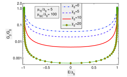
Figure 2: The sub-gap conductance of an $s$-wave SC in units of $G_{0}$, for $\chi_{1}=\chi_{2}=0$. The $G_{3}$-axis is shown on a logarithmic scale to make the distinction between different lines clearer.

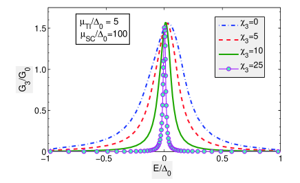
Figure 3: The sub-gap conductance of a $p_{y}$-wave SC in units of $G_{0}$, for $\vec{d}=\hat{z}$ and $\chi_{1}=\chi_{2}=0$.

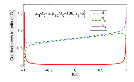
(a)  $s$-wave SC

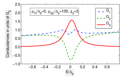
(b)  $p_{y}$-wave SC with $\vec{d}=\hat{z}$

Figure 4: The differential conductances $G_{3}$ into the SC, $G_{2}$ into the TI-2 and $G_{1}$ back to the TI-1 in units of $G_{0}$, for (a) an $s$-wave SC, and (b) a $p_{y}$-wave SC with $\vec{d}=\hat{z}$.

Edge States

To understand the variation of the sub-gap tunneling conductance $G_{3}$ with the barrier potentials $\chi_{1}$ and $\chi_{2}$, we first discuss the localized edge states of the superconductor near the line junction. We note that a SC with a boundary along $y=0$, depending on its pairing symmetry, may exhibit sub-gap localized edge states at the boundary. These states appear at the edges (middle) of the superconducting gap for $s$- ($p$-) wave pairing symmetry hu1 . To understand this, let us first consider a system consisting of only a SC with a hard wall at $y=0$, and study the bound states which can occur in that case; later, we shall discuss the effect that such bound states have on the conductance when the SC is coupled to the two TIs.

The wave function of a bound state will have a factor $e^{i(k_{x}x+k_{y}y-Et/\hbar)}$, where $k_{x}$ and $E$ are real and $Im(k_{y})>0$. Given some real values of $E$ and $k_{x}$, dispersion relation will generally have four solutions for $k_{y}$ of the form $k$, $k^{*}$, $-k$ and $-k^{*}$. Of these we choose the two solutions whose imaginary part is positive. Let us call those solutions $k_{\pm}=\pm k_{R}+ik_{I}$, where $k_{R}$ and $k_{I}$ are positive and denote the corresponding four-component eigenstates of the Hamiltonian by $\Psi_{+}$ and $\Psi_{-}$ for a particular component of the spin. If these eigenstates are identical, then we can take their superposition with opposite signs to obtain a wave function which is proportional to $\Psi_{+}\sin(k_{R}y)e^{i(k_{x}x-Et/\hbar)-k_{I}y}$; this vanishes at $y=0$ thereby satisfying the hard wall boundary condition and giving us a bound state. In general, for a given value of $E$, there will be a particular value of $k_{x}$ for which there are two eigenstates which are identical and can therefore be superposed to give a bound state; hence the bound states will have a dispersion in which $E$ is a function of $k_{x}$. Further, there will be two such states for a given $E$ and $k_{x}$ corresponding to the spin degree of freedom.

Now we discuss the effect that the existence of bound states on the SC-side may have an effect on the conductance when the SC is coupled to two TIs. In general, an electron incident on TI-1 penetrates into the SC up to some distance ($\propto 1/k_{R}$) and the amplitude (hence the transmission probability) for such a penetration can be suppressed by increasing the barrier strength $\chi_{3}$. However, if an electron is incident with an energy which is exactly equal to the bound state energy on the SC side, there will be a resonance in the transmission to the SC side and the barrier $\chi_{3}$ does not affect the transmission. A flat dispersion for the bound state spectrum therefore means that the conductance should be enhanced when the bias matches exactly the bound state energy on SC side. We shall soon see that the bound state spectrum is flat for certain cases. For larger barrier strength $\chi_{3}$, the peak is more visible since a larger barrier will suppress transmission at energies other than the bound state energy. We find such peaks in our numerical calculations for (i) an $s$-wave SC at $E=\pm\Delta$ (see Fig. 2) and (ii) a $p$-wave SC at $E=0$ (see Fig. 3) as expected hu1 .

$s$-wave SC: The wave function $\Psi_{3}$ for an $s$-wave SC is given by Eq. (79). We find that the wave function $\Psi_{3}$ consistent with the hard wall boundary exists only when $E=\pm\Delta$. The dispersion for the bound states is flat $E=\pm\Delta$ for any $k_{x}$. These bound states are responsible for the sub-gap conductance peaks at $E=\pm\Delta$ in Fig. 2. At $E=\Delta$, $\eta=0$ and hence $\Psi_{3}$ and $\partial_{y}\Psi_{3}$ can be written as a linear combination of the spinors $[1~{}0~{}0~{}1]^{T}$ and $[0~{}~{}1~{}-1~{}~{}0]^{T}$. So if we multiply Eqs. (29) from the left by the orthogonal row vectors $[1~{}~{}0~{}~{}0~{}-1]$ and $[0~{}1~{}1~{}0]$, the boundary condition reduces to four equations with four unknowns $t_{N}$, $t_{A}$, $r_{N}$ and $r_{A}$ which can easily be solved. (The details of a similar calculation for a $p$-wave SC are presented in the Appendix). The important point to note here is that the barrier strength $\chi_{3}$ drops out of the problem. Let us choose $\chi_{1}=\chi_{2}=0$ for simplicity. We find that $t_{N}=t_{A}=0$ and

$$|r_{A}|^{2}=\frac{1-\cos{\theta_{1}}}{1+\cos{(\theta_{1}+\theta_{1h})}}.$$ (103)

A similar calculation yields the same expression for the scattering probabilities for the case $E=-\Delta$. However the difference to note is that $\theta_{1h}$ is different at energies $E=\pm\Delta$ since $\cos{\theta_{1h}}=\cos{\theta_{1}}~{}(\mu_{TI}+E)/(\mu_{TI}-E)$. Numerically, we find that the conductance $G_{3}$ approximately obeys $G_{3}(\Delta)=G_{3}(-\Delta)$ in the limit $\mu_{SC}\gg\Delta$.

$p$-wave SC: Let us study a $p$-wave SC with the choice $f(\vec{k})=k_{y}/k_{F}$ and $\vec{d}=\hat{z}$. For this case, the wave function $\Psi_{3}$ given by Eq. (99) is consistent with the hard wall boundary only when $w=-w^{*}$ which simplifies to

$$\Big{[}E-\frac{\hbar^{2}(k_{x}^{2}+k_{R}^{2})}{2m}+\mu_{SC}\Big{]}k_{R}=0$$ (104)

We find that the bound state dispersion is flat: $E=0$ for all $k_{x}$. [However when $f(\vec{k})\propto k_{y}+i\alpha k_{x}$, with a non-zero $\alpha$, the bound states have a dispersion owing to TRS breaking]. From the calculation detailed in the Appendix, we see that for $E=0$, $r_{A}=t_{N}=0$,

$$|t_{A}|^{2}=\frac{1-\cos{2\theta_{1}}}{1+\sin^{2}{\theta_{1}}+\cos^{2}{\theta_{1}}~{}\sin{[2(\chi_{1}-\chi_{2})]}},$$ (105)

and $|r_{N}|^{2}=1-|t_{A}|^{2}$. Remarkably, $|t_{A}|^{2}$ and hence the mid-gap conductance $G_{3}(0)$ depend only on the difference $\chi_{1}-\chi_{2}$. [This is in contrast to the conductance of a junction of just two topological insulators (i.e., our set-up without the SC side) where the total barrier strength seen by the electrons is $\chi_{1}+\chi_{2}$; then the conductance will only depend on $\chi_{1}+\chi_{2}$]. The important result that $|t_{A}|^{2}$ depends only on the combination $\chi_{1}-\chi_{2}$ (and hence $G_{3}$ also, since $r_{A}=0$) at zero bias can be understood qualitatively as follows. An electron incident on the junction from the TI-1 side sees a barrier strength of $\chi_{1}$ on that side. It then transmits to the TI-2 side with an amplitude $t_{A}$ as a hole; such a hole sees a barrier strength of $-\chi_{2}$ on that side, since the potentials seen by electrons and holes have opposite signs. Hence the total barrier strength seen is given by $\chi_{1}-\chi_{2}$; hence this is the parameter which appears in Eq. (105).

The numerical results shown in Fig. 5 highlight these features. To illustrate the behavior of conductance as a function of different barrier strengths, we choose $\chi_{1}=\chi_{2}=\chi_{3}=\chi$. At non-zero bias, the conductance has periodic oscillations with a decaying envelope as shown in Fig. 5 (a). The periodic oscillations are due to the barriers $\chi_{1}$ and $\chi_{2}$ on the TI surfaces while the decaying envelope is due to the barrier $\chi_{3}$ on the SC side. At zero bias (i.e., $E=0$), the barrier on the SC side no more plays a role in determining the conductance as we saw analytically earlier. However, the barriers $\chi_{1}$ and $\chi_{2}$ on the TI side together determine the value of the ZBP. The numerical results in Fig. 5 (a) for $\chi_{2}=\chi_{1}$ and (b) for $\chi_{2}=-\chi_{1}$ show that the value of $G_{3}$ at $E=0$ is a function of $\chi_{1}-\chi_{2}$ only.

(a)   $\chi_{1}=\chi_{2}$,  $\vec{d}=\hat{z}$

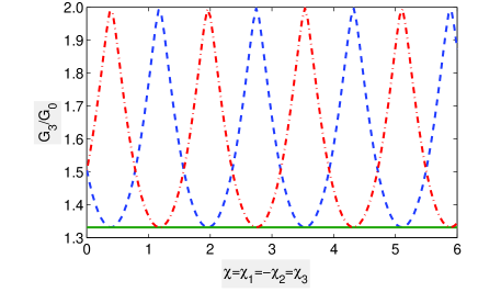
(b)   $\chi_{1}=-\chi_{2}$, $E=0$

Figure 5: (a) Conductance of a $p_{y}$-wave SC with $\vec{d}=\hat{z}$ at different energies in the SC gap. (b) Conductance of a $p_{y}$-wave SC at $E=0$ for different spin pairings: $\vec{d}=\hat{z}$ (blue dashed line), $\vec{d}=\hat{x}$ (green solid line) and $\vec{d}=\hat{y}$ (red dot-dashed line). Note that $G_{3}/G_{0}$ reaches 2 at $\chi=n\pi/2+3\pi/8$ for $\vec{d}=\hat{z}$ and at $\chi=n\pi/2+\pi/8$ for $\vec{d}=\hat{y}$, as can be shown from Eqs. (105) and (106).

For a $p$-wave SC, when $\vec{d}=\hat{x}$ or $\vec{d}=\hat{y}$, we find that the dependence of the conductance on the bias is different from that for $\vec{d}=\hat{z}$ shown in Fig. 3. For the case $\vec{d}=\hat{y}$, we again find that $r_{A}=t_{N}=0$ while

$$|t_{A}|^{2}=\frac{1-\cos{2\theta_{1}}}{1+\sin^{2}{\theta_{1}}-\cos^{2}{\theta_{1}}~{}\sin{[2(\chi_{1}-\chi_{2})]}}.$$ (106)

(The qualitative reason for the dependence on $\chi_{1}-\chi_{2}$ is similar to the one given above for $\vec{d}=\hat{z}$). For the case $\vec{d}=\hat{x}$, we find that $t_{A}=t_{N}=0$, while

$$|r_{A}|^{2}=\sin^{2}{\theta_{1}}$$ (107)

and $|r_{N}|^{2}=\cos^{2}\theta_{1}$ are independent of $\chi_{1}$ and $\chi_{2}$. This independence stems from following reason: an electron incident on the junction from the TI-1 side sees a barrier strength of $\chi_{1}$. When it is Andreev reflected as a hole back to that side, it sees a barrier strength of $-\chi_{1}$. Hence the total barrier strength that is seen is zero, regardless of the value of $\chi_{1}$. Further, there is no dependence on $\chi_{2}$ since the electrons does not transmit to the TI-2 side at all; both $t_{A}$ and $t_{N}$ are zero.

These analytical results are confirmed by our numerical calculations. This is illustrated in Fig. 5 (b) where $G_{3}$ is plotted as a function of $\chi_{1}-\chi_{2}$ at $E=0$ for the three different forms of $\vec{d}$. Note that for $\vec{d}=\hat{y}$ and $\hat{z}$, $G_{3}$ varies with a period of $\pi/2$ in the variable $\chi=(\chi_{1}-\chi_{2})/2$ in Fig. 5 (b). This is in agreement with Eqs. (105) and (106) which are periodic in $\chi_{1}-\chi_{2}=\pi$. We note that our results demonstrate that the barrier dependence of the sub-gap tunneling conductance of junctions of TI and triplet superconductors can be used to determine the direction of the direction of ${\vec{d}}$, or equivalently, the direction of the spin of the Cooper pair. This property is in complete contrast to the conventional NM-SC junctions and stems from the spin-momentum locking of the Dirac electrons which breaks the rotational symmetry in the spin space necessary to distinguish between the different orientation of ${\vec{d}}$.

For a $p$-wave SC, we can in general take $f(\vec{k})\propto k_{y}+i\alpha k_{x}$. The choice $\alpha=0$ corresponds to $p_{y}$-SC and the bound state dispersion is flat as discussed earlier. When $\alpha$ is changed slightly from zero, we find that the bound state dispersion develops a small non-zero slope. Now, the ZBP which existed for $\alpha=0$ broadens and the peak value also decreases; the peak eventually disappears as $\alpha$ is increased further.

VI Spin Currents

In this section we will study the spin currents on the SC side for $s$- and $p$-wave cases. For $a=x,y,z$, the $a$ component of the spin density is given by

$$\rho_{a}~{}=~{}\frac{\hbar}{2}~{}\Psi_{3}^{\dagger}\tau^{z}\otimes\sigma^{a}\Psi_{3}$$ (108)

in the four-component language. The operator $\tau^{z}$ appears in Eq. (108) because a hole with spin-up (down) corresponds to a missing electron with spin-down (up). The spin current $\vec{J}_{a}$ corresponding to the spin density $\rho_{a}$ can be calculated on the SC side using the equations of motion Eq. (16) and (17) and the continuity equation $\partial_{t}\rho_{a}+\vec{\nabla}\cdot{\vec{J}_{a}}=0$. The equation of continuity implies that in a steady state, the component ${\hat{y}}\cdot{\vec{J}_{a}}$ is independent of the $y$ coordinate and can therefore be evaluated at any convenient point like $y=0$ or $\infty$. We are interested in only the $\hat{y}$ component of the $a$-spin currents since only this component contributes to the spin density that is injected into the SC. The differential spin conductance $G^{s}_{a}$ corresponding to the spin density $\rho_{a}$ is obtained by integrating over the spin current contributions ${\hat{y}}\cdot{\vec{J}_{a}}$ from all the angles of incidence $0<\theta_{1}<\pi$ :

$$G^{s}_{a} = G^{s}_{0}~{}\gamma_{E}~{}\Big{[}\frac{k_{F}}{\mu_{SC}}\int_{0}^{\pi}d\theta_{1}~{}\hat{y}\cdot\vec{J}_{a}\Big{]}$$ (109)

where $G^{s}_{0}=\frac{e}{h}~{}\frac{W\mu_{TI}}{hv_{1}^{2}}~{}\frac{\mu_{SC}}{k_{F}}$. Here $G^{s}_{0}$ has been defined in such a way that the term in the brackets in the above equation becomes dimensionless.

In a normal metal, i.e., setting $\Delta_{0}=0$ in Eq. (16), we find that

$$\vec{J}_{a}~{}=~{}\frac{\hbar^{2}}{2m}~{}Im[\Psi_{3}^{\dagger}\sigma^{a}\vec{\nabla}\Psi_{3}].$$ (110)

In a SC, the spin current $\vec{J}_{a}$ is a sum of two parts: the part $\vec{J}_{a,N}$ which is independent of $\Delta_{0}$ given by Eq. (110), and the part $\vec{J}_{a,\Delta}$ proportional to $\Delta_{0}$. $\vec{J}_{a,N}$ is the expression for the $a$-spin current in a normal metal carried by either electrons or holes; in SC it gets contribution from the BdG quasiparticles. For an $s$-wave SC, we find that the $x$- and $z$- spin currents (i.e., $\vec{J}_{a}$ for $a=x,z$) are entirely given by Eq. (110) and do not contain the SC pair potential $\Delta_{0}$ ($J_{x/z,\Delta}=0$). Since the wave function $\Psi_{3}$ decays exponentially as $y\to\infty$, the spin current going into the SC is zero at $y\to\infty$ (and therefore at any value of $y$) if $a=x$ or $z$. But the $y$-spin current in addition to the expression in Eq. (110), also contains a part proportional to $\Delta_{0}$ given by-

$$\hat{y}\cdot\vec{J}_{y,\Delta}=-\Delta_{0}~{}\int_{0}^{y}dy^{\prime}~{}Re[\Psi_{3}^{\dagger}(x,y^{\prime})\tau^{x}\Psi_{3}(x,y^{\prime})].$$ (111)

The derivation of this is similar to that of Eq. (LABEL:jpair). Hence the total spin current is given by the sum of Eqs. (110) and (111), and this need not vanish. It is easiest to evaluate this at $y=0$ where Eq. (111) vanishes. For $a=y$, after tedious calculation, we find that Eq. (110) simplifies to

$$\hat{y}\cdot\vec{J}_{y}=\frac{\hbar^{2}k_{R}}{2m}(1+|w|^{2})~{}Im[t_{1}^{*}t_{2}-t_{3}^{*}t_{4}].$$ (112)

The above quantity is non-zero for the scattering of an electron incident at energy $E$, at an angle $\theta_{1}$ on TI-1. But the $\hat{y}\cdot\vec{J}_{y}$ currents at incident angles $\theta_{1}$ and $\pi-\theta_{1}$ add up to zero, thus contributing nothing to the differential spin conductance $G^{s}_{y}$. To summarize, all the spin conductances $G^{s}_{a}$ are zero for the $s$-wave case.

For a $p$-wave SC, the $a$-spin current is given by

$$\vec{\nabla}\cdot\vec{J}_{a,\Delta}=\Delta_{0}~{} Re\Big{[} \vec{a}\cdot[\psi^{\dagger}\sigma^{a}(\vec{d}\cdot\vec{\sigma})i\sigma^{y}\vec{\nabla}\phi$$ (113)

$$-\vec{\nabla}\psi^{\dagger}(\vec{d}\cdot\vec{\sigma})i\sigma^{y}\sigma^{a}\phi]\Big{]}.$$

We will now consider all the nine different possibilities corresponding to $\vec{d}=\hat{x},\hat{y},\hat{z}$ and $a=x,y,z$. Table 1 summarizes the results for different spin currents, while Table 2 summarizes the spin conductance results (obtained by integrating out spin currents over all incident angles $\theta_{1}$) for different cases. For the four cases corresponding to $(\vec{d},a)=(\hat{x},x)$, $(\hat{x},y)$, $(\hat{z},y)$ and $(\hat{z},z)$, we find that $\vec{\nabla}\cdot\vec{J}_{a,\Delta}$ is a total derivative, which implies that $\vec{J}_{a,\Delta}$ has a local expression in terms of $\Psi_{3}$ (analogous to the last terms in Eq. (24)). Then one can evaluate both $\vec{J}_{a,\Delta}$ and Eq. (110) at $y=\infty$; they vanish there because $\Psi_{3}$ goes to zero exponentially. Hence no spin current enters the SC in these four cases. In the remaining five cases, we find that $\vec{\nabla}\cdot\vec{J}_{a,\Delta}$ is not a total derivative; hence $\vec{J}_{a,\Delta}$ has an integral expression (analogous to Eq. (111)). Since this vanishes at $y=0$, one can find the total spin current by evaluating only Eq. (110) at $y=0$.

	$s$-wave	$p$-wave	$p$-wave	$p$-wave
		$\vec{d}=\hat{x}$	$\vec{d}=\hat{y}$	$\vec{d}=\hat{z}$
$J_{x}$	0	0	Eq. (115)	Eq. (115)
$J_{y}$	Eq. (112)	0	Eq. (116)	0
$J_{z}$	0	Eq. (114)	Eq. (114)	0

Table 1: Expressions for spin currents for $s$-wave and $p$-wave pairing for a particular angle of incidence.

	$s$-wave	$p$-wave	$p$-wave	$p$-wave
		$\vec{d}=\hat{x}$	$\vec{d}=\hat{y}$	$\vec{d}=\hat{z}$
$G^{s}_{x}$	0	0	non-zero	non-zero
$G^{s}_{y}$	0	0	0	0
$G^{s}_{z}$	0	0	0	0

Table 2: Spin conductances $G^{s}_{a}$ for $s$-wave and $p_{y}$-wave SC.

$\vec{d}=\hat{x}$ : As argued earlier, no $a$-spin current corresponding to $a=x,y$ enters the SC. $J_{z}$ on the other hand has an expression given by

$$\hat{y}\cdot\vec{J}_{z}=\frac{\hbar^{2}k_{R}}{4m}(1+|w|^{2})~{}[|t_{1}|^{2}-|t_{2}|^{2}-|t_{3}|^{2}+|t_{4}|^{2}]~{}.$$ (114)

This is the expression for $z$-spin current for electron incident at a given energy $E$ and angle $\theta_{1}$ on TI-1. The $z$-spin conductance on SC is obtained by summing up the currents at all possible incident angles $0<\theta_{1}<\pi$. The $z$-spin conductance $G^{s}_{z}$ turns out to be zero due to the exact cancellation of the $\hat{y}\cdot\vec{J}_{z}$ at angles $\theta_{1}$ and $\pi-\theta_{1}$.

$\vec{d}=\hat{y}$ : All the three spin currents could have a non-zero value in this case (see Table 1). The expression for $z$-spin current in this case is given by Eq. (114) and the total $z$-spin current at any given energy $E$ in the gap goes to zero by the same logic that follows Eq. (114). The expressions for the $x/y$-spin currents are

$$\hat{y}\cdot\vec{J}_{x}=\frac{\hbar^{2}k_{R}}{2m}(1+|w|^{2})~{}Re[t_{1}^{*}t_{2}-t_{3}^{*}t_{4}],$$ (115)

$$\hat{y}\cdot\vec{J}_{y}=\frac{\hbar^{2}k_{R}}{2m}(1+|w|^{2})~{}Im[t_{1}^{*}t_{2}-t_{3}^{*}t_{4}].$$ (116)

Integrating the spin current over $\theta_{1}$, we find that the $y$-spin conductance is zero while the $x$-spin conductance is non-zero and has features similar to the $\vec{d}=\hat{z}$ case as discussed below.

$\vec{d}=\hat{z}$ : In this case as argued earlier, $y/z$-spin currents are zero. The expression for $x$-spin current is given by Eq. (115). The spin conductance which is integrated over $x$-spin current is non-zero and has some feature as shown in Fig. 6 for a typical case.

If we compare Tables 1 and 2, the non-zero $y$($z$)-spin current for an electron incident at angle $\theta_{1}$ in Table 1 adds up with the $y$($z$)-spin current for an electron incident at angle $\pi-\theta_{1}$ to give zero in the total $y$($z$)-spin conductance. This can be seen from the symmetry of the equations of motion and the boundary conditions under the transformation $x\to-x$. For both TI-1 and TI-2, the equations of motion (Eq. (15)) remain invariant under the transformations: $\Psi_{i}\to\sigma^{x}\Psi_{i}$ and $\Psi_{i}\to\tau^{z}\sigma^{x}\Psi_{i}$ accompanied by $x\to-x$. Both the boundary conditions Eqs. (29) and Eqs. (33) are invariant under these two transformations. However, for $s$-wave SC and the $p$-wave SC with $\vec{d}=\hat{x}$ the equations of motion (Eq. (16) and Eq. (17)) are invariant under the transformation $\Psi_{3}\to\tau^{z}\sigma^{x}\Psi_{3}$. And for $p$-wave SC with $\vec{d}=\hat{y},~{}\hat{z}$ the equations of motion (Eq. (17)) are invariant under the transformation $\Psi_{3}\to\sigma^{x}\Psi_{3}$. Now, we can easily see from Eq. (110) that under both the transformations ($\Psi_{i}\to\sigma^{x}\Psi_{i}$ and $\Psi_{i}\to\tau^{z}\sigma^{x}\Psi_{i}$), $\hat{y}\cdot\vec{J}_{x}$ is invariant while $\hat{y}\cdot\vec{J}_{y}$ and $\hat{y}\cdot\vec{J}_{z}$ change sign. Since $x\to-x$ is same as $\theta_{1}\to\pi-\theta_{1}$, this explains the exact cancellation of $y$- and $z$-spin currents for $\theta_{1}$ and $\pi-\theta_{1}$.

We can relate the spin currents which are non-zero in Table 2 to the physical quantities on the other side of the junction, i.e., on the TI-1 and TI-2 sides. Using the boundary conditions in Eqs. (33), we can rewrite the $x$-spin current at the junction as

$$\hat{y}\cdot\vec{J}^{SC}_{x}~{}=~{}\frac{\hbar}{2}[v_{1}\Psi_{1}^{\dagger}\tau^{z}\Psi_{1}-v_{2}\Psi_{2}^{\dagger}\tau^{z}\Psi_{2}]$$ (117)

for a $p_{y}$-wave SC with $\vec{d}=\hat{y}$ or $\hat{z}$. We thus see that the $x$-spin current on the SC side of the junction is linearly related to the steady state charge densities on the TI-1 and TI-2 sides of the junction evaluated at the junction.

Spin Conductance

The $x$-spin conductance shows an unusual satellite peak (SP) in addition to the ZBP for the cases $\vec{d}=\hat{y}$ and $\vec{d}=\hat{z}$ when $f(\vec{k})=k_{y}/k_{F}$ (see Fig. 6). This SP merges with the ZBP for $\chi_{3}\gtrsim 20$. The SP is observable only if there is an appreciable penetration of a plane wave state with non-zero energy from the TI-1 into the SC, and this can occur only if $\chi_{3}$ is not too large. The location and height of the SP change with $\chi_{1}$ and $\chi_{2}$ in a periodic way. To highlight these features, we choose $\chi_{1}=\chi_{2}=\chi_{3}\equiv\chi$ and show the spin conductance $G^{s}_{x}$ as a function of the bias and the barrier strength $\chi$ in Fig. 7 as a contour plot.

We find, using Eq. (117), that the $x$-spin current in the superconductor can be written in terms of the charge densities in TI-1 and TI-2. In the case $v_{1}=v_{2}$, we find that the spin current is proportional to $\Psi_{1}^{\dagger}\tau^{z}\Psi_{1}-\Psi_{2}^{\dagger}\tau^{z}\Psi_{2}$ which is given by

$$\Psi_{1}^{\dagger}\tau^{z}\Psi_{1}-\Psi_{2}^{\dagger}\tau^{z}\Psi_{2}$$

$$=1+R_{N}+R_{N,Ph}-R_{A}\Gamma_{1A}-T_{N}+T_{A}\Gamma_{2A},$$ (118)

where

$$R_{N,Ph} = Re(r_{N}+r_{N}e^{-i2\theta_{1}}),$$

$$\Gamma_{1A} = \nu_{E}^{2}\cos^{2}{\theta_{1}}-\nu_{E}\cos{\theta_{1}}\sqrt{\nu_{E}^{2}\cos^{2}{\theta_{1}}-1},$$

$$\Gamma_{2A} = |\nu_{E}\cos{\theta_{1}}|,$$ (119)

in the range of $(E,\theta_{1})$ for which there exist evanescent Andreev modes on TI-1 and TI-2, i.e., when $\nu_{E}\cos{\theta_{1}}>1$. When the Andreev states are plane wave states on TI-1 and TI-2, $\Gamma_{1A}$ and $\Gamma_{2A}$ both are equal to $1$ in Eq. (118).

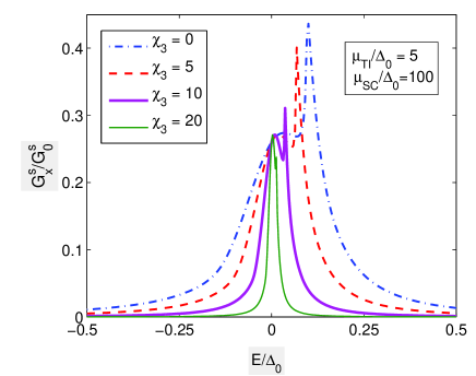
Figure 6: Spin conductance for a $p_{y}$-wave SC with $\vec{d}=\hat{z}$ and $\chi_{1}=\chi_{2}=0$. There is a satellite peak at a positive value of the bias which merges with the ZBP in the limit of large $\chi_{3}$.

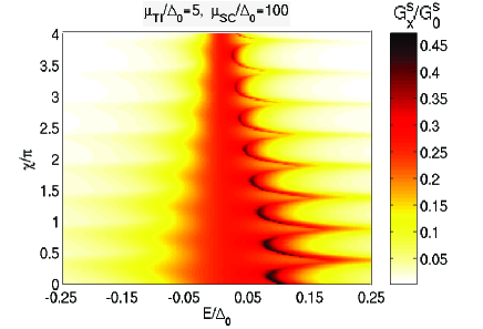
Figure 7: Spin conductance for a $p_{y}$-wave SC with $\vec{d}=\hat{z}$ and $\chi_{1}=\chi_{2}=\chi_{3}=\chi$. Both the location and the height of the SP oscillate and decay with increasing $\chi$.

Using the identity in Eq. (118), we find the contributions to the spin conductance $G_{x}^{s}$ from the different scattering amplitudes on the TI-1 and TI-2 sides. It is interesting to note that in contrast to the expressions in Eq. (102) for the charge conductances where only the scattering probabilities in the TI-1 and TI-2 appear, the spin conductance on SC side depends both on the phase and the amplitude of the reflection amplitude $r_{N}$. We show in Fig. 8 the contributions to the spin conductance from the different terms in Eq. (118). From the figure, it is evident that the Andreev scattering term $(T_{A}\Gamma_{2A}-R_{A}\Gamma_{1A})$ and the term $R_{N,Ph}$ (which is proportional to $r_{N}$) contribute the most to the SP. Further, to understand the origin of the SP, we look at the spin currents due to incident electrons with different energies and angles of incidence $\theta_{1}$. In Fig. 9, we show spin conductances at different $E$ and $\theta_{1}$ as a contour plot. This contour plot shows that the ZBP and the SP in the spin conductance get contributions from different angles $\theta_{1}$. In contrast to the ZBP in the spin conductance which gets contributions mainly around normal incidence ($\theta_{1}\sim\pi/2$), the SP gets major contributions from electrons incident at glancing angles ($\theta_{1}\sim 0$ and $\theta_{1}\sim\pi$). This is highlighted in the contour plot by ellipses. The green (dot-dash) lines, $\theta_{1}=\cos^{-1}(\pm 1/\nu_{E})$, separate the evanescent Andreev modes on TI-1 and TI-2 from the Andreev plane wave states. The largest contribution to the SP comes from the range of $\theta_{1}$ for which there are evanescent Andreev modes; this is shown by the pink (dark) region in the contour plot. In the same region, we find that the phase of $r_{N}$ changes rapidly from $-\pi$ to $\pi$ (going through $0$) as $E$ is varied at a fixed value of $\theta_{1}$. Such a feature in the phase of $r_{N}$ shows up as a peak in the term $R_{N,Ph}$ in Eq. (118) when $E$ is varied at a fixed $\theta_{1}$. Further, the SP in spin conductance merges with the ZBP in the limit $\mu_{SC}\to\infty$.

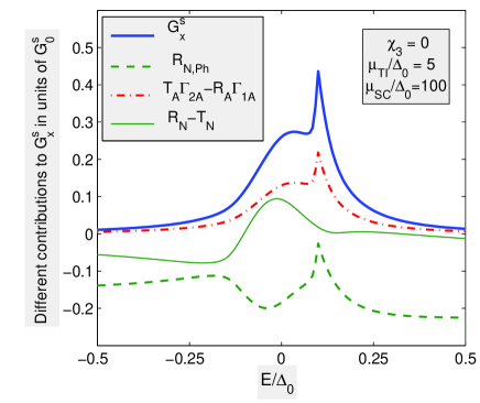
Figure 8: Spin conductance and the contributions from different terms in Eq. (118) for a $p_{y}$-wave SC with $\vec{d}=\hat{z}$ and $\chi_{1}=\chi_{2}=\chi_{3}=0$. The phase term $R_{N,Ph}$ and the Andreev terms $T_{A}\Gamma_{2A}-R_{A}\Gamma_{1A}$ contribute to the SP.

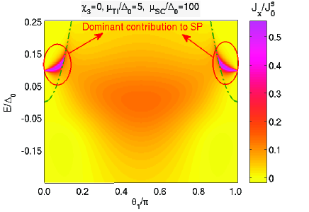
Figure 9: Contour plot of spin current $\hat{y}\cdot\vec{J}_{x}$ (in units of $J^{s}_{0}=\hbar^{2}k_{F}/(2m)$) as a function of the energy and incident angle of the electron on the TI-1 side, for a $p_{y}$-wave SC with $\vec{d}=\hat{z}$ and $\chi_{1}=\chi_{2}=\chi_{3}=0$. The dominant contribution to the SP comes from the pink (dark) regions which are bounded by the green dot-dash lines. See text for details.

There is a striking asymmetry about $E=0$ in the spin conductance in Fig. 6; this mainly arises because the evanescent Andreev modes can exist only for $E>0$ and are absent for $E<0$. There is also an asymmetry due to a finite difference in the density of states of the incident electrons at energies $E$ and $-E$ (see Eq. (102)) and the lack of invariance of Eq. (99) under $E\to-E$. A small asymmetry is also visible in the charge conductance shown in Fig. 3.

VII Summary and Discussion

In this paper, we have considered a junction between two TIs and a SC which can be either $s$-wave or $p$-wave; a $p$-wave SC may have different spin pairings and we have studied each case. We have formulated the most general time-reversal invariant boundary condition at the junction; this consists of three barrier parameters. We have studied the dependence of the differential charge and spin conductances on the barrier parameters, the ratio of the TI and SC chemical potentials to the superconducting pair potential, and the voltage bias.

Our main results can be summarized as follows.

(i) In accordance with conventional NM-SC junctions, we find that the charge conductance $G_{3}$ shows peaks at the edges of the SC gap for $s$-wave SC; for a $p$-wave SC, there is a peak at the zero bias. However, in contrast to conventional junctions, the heights of these peaks do not reach the conventional value of $2G_{0}$, if $\chi_{1}=\chi_{2}=0$; this feature is a signature of the Dirac nature of the TI quasiparticles. Further, the height of these peaks is independent of $\chi_{3}$. The conductance peaks arise due to the presence of bound states on the SC side; as a result, an electron coming in from the TI side with the same energy as the bound state can resonantly enter the SC, and then convert into Cooper pairs deep inside the SC. (The phenomenon of a conductance peak resembles the transmission resonance which occurs in other systems; see Ref. reso, for a few examples).

(ii) For a $p$-wave SC, we studied the conductance as a function of barrier strengths. At non-zero energies the conductance both oscillates and decreases with increasing barrier strength. This demonstrates both the Dirac and the Schrödinger nature of the electrons in different parts of our set-up in the following sense. The transmission of Dirac electrons oscillates with the barrier strengths in the TI-1 and TI-2 (as can be seen by the presence of $\cos\chi_{i}$ and $\sin\chi_{i}$ terms in the boundary conditions (29) and (33), for $i=1,2$), while the transmission of Schrödinger electrons through the barrier in the SC decays exponentially with the barrier strength $\chi_{3}$. This indicates that for $\chi_{1}=\chi_{2}=0$ the charge conductance in these junctions does not reach the maximum value of $2G_{0}$ which is found in conventional junctions.

(iii) For a $p$-wave SC, the dependence of the conductance on the barrier parameters (specifically on the difference of the parameters in the two TIs, $\chi_{1}-\chi_{2}$, at zero bias) varies with the direction of $\vec{d}$, i.e., the spin pairing of the Cooper pairs. This is due to the spin-momentum locking of the electrons in the TIs and the fact that the geometrical arrangement of the two TIs completely breaks the rotational symmetry. This is quite different from what happens in a junction of normal metals with a $p$-wave SC; since a metal is isotropic in spin space, the conductance into a SC would not depend on the direction of $\vec{d}$. Thus these junctions are expected to provide a test bed for determining the orientation of $\vec{d}$ and hence the Copper pair spin direction of triplet SC without application of external magnetic fields mack .

(iv) The spin conductance into the SC for different pair potentials exhibits several unconventional features. We find that there is a non-zero conductance for the $x$ component of the spin only for a $p_{y}$-wave SC in which $\vec{d}=\hat{y}$ or $\hat{z}$. (The fact that all the other spin conductances are zero can be shown using a parity symmetry which is present in our system). The non-zero spin conductance arises because the TIs break the spin rotation symmetry, and it does not occur for a NM-SC junction. Most remarkably, the spin conductance shows a satellite peak away from zero energy. We have provided an explanation of this satellite peak by relating the spin conductance on the SC side to the charge densities on the TI sides. The charge density turns out to depend on the phase of the normal reflection amplitude which shows a peak at non-zero bias. The satellite peak in the spin conductance is a distinctive feature of our system and it would be interesting to look for this experimentally.

The simplest experimental verification of our theory would be to measure the maxima of the charge conductance peaks for both $s$- and $p$-wave SCs. A prediction of our theory is that the values of these peaks reach $2G_{0}$ only for some non-zero barrier strengths. It will also be interesting to measure the barrier potential dependence of $G_{3}$. The barrier potentials can be tuned by applying a gate voltage along the junction in our system. It may be difficult to tune $\chi_{1}$, $\chi_{2}$ and $\chi_{3}$ separately. Looking at Fig. 1, however, it is apparent that if a gate voltage is applied from above the junction, it will have a larger effect on $\chi_{1}$ and $\chi_{3}$ than on $\chi_{2}$ (since it is further away from the TI-2); hence changing such a gate voltage will change the value of $\chi_{1}-\chi_{2}$. Hence our important prediction that the zero bias peak depends on $\chi_{1}-\chi_{2}$ for $\vec{d}=\hat{y}$ and $\hat{z}$ but does not depend at all on any of the $\chi_{i}$ for $\vec{d}=\hat{x}$ is something which can be tested by changing the gate voltage. A consequence of this would be that measurements of $G_{3}$ can be used to determine the direction of $\vec{d}$ for a given $p$-wave SC by attaching it to a junction of two TIs.

Recently, there has been much excitement about a zero-bias peak (ZBP) observed in a number of experiments in semiconducting/superconducting nanowires mourik ; deng ; rokhinson ; das . This peak is believed to be due to a Majorana fermion mode, and it has a close connection to the mid-gap (zero energy) states which are present at the boundary of a $p$-wave SC kseng01 ; kseng02 ; kwon . The last few years have witnessed intense theoretical activity in the area of Majorana modes at the ends of one-dimensional systems lutchyn1 ; oreg ; brouwer1 ; degottardi ; potter ; fulga ; stanescu ; tewari ; gibertini ; lim ; tezuka ; egger ; ganga ; lobos ; lutchyn2 ; fidkowski ; cook ; pedrocchi ; sticlet ; jose ; klinovaja ; alicea . In our system, we have studied the edge states which occur at $E=0$ in a $p$-wave SC with a hard wall. However, although these states give rise to a zero bias peak in the charge conductance, they cannot be called Majorana modes for the following reason. A Majorana mode must have a real wave function so that it remains invariant under complex conjugation. However, our zero energy states carry finite momentum $k_{x}$ and do not have real wave functions. Under complex conjugation, a state with momentum $k_{x}$ changes to a state with momentum $-k_{x}$ and therefore does not remain invariant.

Finally, we point out that in this work we have studied the charge and spin conductances of a junction between two TI surfaces and one SC. It is natural to ask what would happen if there was a junction of a single TI surface and an SC. A peculiarity of this problem would be that a single TI has only one spin degree of freedom for a given value of the energy and momentum, while a SC (or metal) has two spin degrees of freedom. Hence boundary conditions such as the ones given in Eqs. (29-33) would generally be inconsistent since they provide eight equations for six amplitudes (normal and Andreev reflection in the TI and four amplitudes on the SC side). For our system with two TIs and a SC, there is no such mismatch. This enables us to find all the amplitudes for all values of the system parameters, and the amplitudes always satisfy the conservation of probability.

Appendix

Here, we shall present a calculation to show how different scattering amplitudes become independent of the barrier $\chi_{3}$ on the SC side when the SC side hosts bound states. In particular, we choose to discuss the case of $p_{y}$-SC with $\vec{d}=\hat{z}$, and $v_{1}=v_{2}$ in the TIs.

From the Hamiltonian in Eq. (LABEL:HSC), it is easy to see that for a $p_{y}$-SC with $\vec{d}=\hat{z}$, $w$ defined in Eq. (99) satisfies the $2\times 2$ matrix equation

$$\Big{[}\Big{(}\frac{\hbar^{2}(k_{x}^{2}+k_{y}^{2})}{2m}-\mu_{SC}\Big{)}\tau^{z}+\frac{\Delta_{0}k_{y}}{k_{F}}\tau^{x}\Big{]}\left(\begin{array}[]{c}1\\ w\end{array}\right)=E\left(\begin{array}[]{c}1\\ w\end{array}\right).$$ (120)

At $E=0$ we can see that the two rows of this equation imply that $w^{2}=-1$. Further, $k_{y}=k_{ySC}$ given by Eq. (80) can be written as $k_{y}=k_{R}+ik_{I}$ with $k_{I}>0$. With this, it is easy to see that $w=-i$. Then, Eq. (99) shows that the wave function on the SC side $\Psi_{3}(y)$ and its derivative $\partial_{y}\Psi_{3}(y)$ both reduce to a linear combination of only the two spinors $\Psi_{p\uparrow}=[1~{}~{}0~{}~{}0~{}-i]^{T}$ and $\Psi_{p\downarrow}=[0~{}~{}1~{}-i~{}~{}0]^{T}$. Also, the third term on the left hand side (LHS) of the second boundary condition in Eqs. (33) will be a linear combination of the spinors $\Psi_{p\uparrow}$ and $\Psi_{p\downarrow}$ for a $p_{y}$-SC with $\vec{d}=\hat{z}$. Hence the LHS of both the equations in the boundary condition in Eqs. (33) are linear combinations of the spinors $\Psi_{p\uparrow}$ and $\Psi_{p\downarrow}$. Since both $\Psi_{p\uparrow}^{T}$ and $\Psi_{p\downarrow}^{T}$ are orthogonal to $\Psi_{p\uparrow}$ and $\Psi_{p\downarrow}$, multiplying by $\Psi_{p\uparrow}^{T}$ and $\Psi_{p\downarrow}^{T}$ from the left in Eqs. (33) makes the LHS equal to zero; hence the equations become independent of $\chi_{3}$. We then get the following four equations containing four unknowns $r_{N}$, $r_{A}$, $t_{N}$ and $t_{A}$,

$$\Psi_{p\uparrow}^{T}\big{[}M(\chi_{1})\Psi_{1}+M(-\chi_{2})\Psi_{2}\big{]} = 0,$$

$$\Psi_{p\downarrow}^{T}\big{[}M(\chi_{1})\Psi_{1}+M(-\chi_{2})\Psi_{2}\big{]} = 0,$$

$$\Psi_{p\uparrow}^{T}\sigma^{x}\tau^{z}\big{[}M(\chi_{1})\Psi_{1}-M(-\chi_{2})\Psi_{2}\big{]} = 0,$$

$$\Psi_{p\downarrow}^{T}\sigma^{x}\tau^{z}\big{[}M(\chi_{1})\Psi_{1}-M(-\chi_{2})\Psi_{2}\big{]} = 0,$$ (121)

where $\Psi_{1}$ and $\Psi_{2}$ are evaluated at $y=0$. When $\Psi_{1}$ and $\Psi_{2}$ from Eqs. (47) and (59) are substituted in the above equations, we get four equations in four unknowns $r_{N}$, $r_{A}$, $t_{N}$ and $t_{A}$ which can be cast in the matrix form: ${\mathds{M}}\cdot X=A$ where

$${\mathds{M}} = \left[\scalebox{0.8}{\mbox{$\displaystyle\begin{array}[]{c c c c}g(\chi_{1})&-w\gamma_{\theta 1}^{*}g^{*}(\chi_{1})&h(\chi_{2})&wh^{*}(\chi_{2})\\ -\gamma_{\theta 1}^{*}g^{*}(-\chi_{1})&wg(-\chi_{1})&-ih(\frac{\pi}{2}+\chi_{2})&-iwh(\frac{\pi}{2}-\chi_{2})\\ -\gamma_{\theta 1}^{*}g^{*}(-\chi_{1})&-wg(-\chi_{1})&ih(\frac{\pi}{2}+\chi_{2})&-iwh(\frac{\pi}{2}-\chi_{2})\\ g(\chi_{1})&w\gamma_{\theta 1}^{*}g^{*}(\chi_{1})&-h(\chi_{2})&wh^{*}(\chi_{2})\\ \end{array}$}}\right],$$ (126)

$$X = \scalebox{1.0}{\mbox{$\displaystyle[r_{N}~{}~{}~{}r_{A}~{}~{}~{}t_{N}~{}~{}~{}t_{A}]^{T}$}},$$

$$A = [\scalebox{0.8}{\mbox{$\displaystyle-g^{*}(\chi_{1})~{}~{}-ig^{*}(\frac{\pi}{2}+\chi_{1})~{}~{}-ig^{*}(\frac{\pi}{2}+\chi_{1})~{}~{}-g^{*}(\chi_{1})$}}]^{T},$$

$${\rm and} g(\chi)~{}=~{}\cos{\chi}+i\gamma_{\theta_{1}}\sin{\chi},~{}~{}~{}~{}\gamma_{\theta_{1}}=-ie^{i\theta_{1}},$$

$${\rm and} h(\chi)=\sqrt{1+\cos{\theta_{1}}}~{}\cos\chi+i\sqrt{1-\cos{\theta_{1}}}~{}\sin\chi.$$ (127)

This set of linear equations yields $r_{A}=t_{N}=0$,

$$|t_{A}|^{2}=\frac{1-\cos{2\theta_{1}}}{1+\sin^{2}{\theta_{1}}+\cos^{2}{\theta_{1}}~{}\sin{[2(\chi_{1}-\chi_{2})]}},$$ (128)

and $|r_{N}|^{2}=1-|t_{A}|^{2}$. The cases $\vec{d}=\hat{x}$ and $\hat{y}$ follow a similar calculation, and the results are given in Eqs. (106) and (107).

For a $s$-wave SC, a similar calculation can be done at $E=\pm\Delta_{0}$; once again, the existence of a bound state on the SC side with a hard wall boundary makes two eigenspinors of the SC Hamiltonian identical. Therefore, there are two other spinors which are orthogonal to these eigenspinors and one can use them to reduce the problem to four equations in four unknowns as shown above.

References

- (1)
- (2) B. A. Bernevig, T. L. Hughes, and S.-C. Zhang, Science 314, 1757 (2006); B. A. Bernevig and S.-C. Zhang, Phys. Rev. Lett. 96, 106802 (2006).
- (3) C. L. Kane and E. J. Mele, Phys. Rev. Lett. 95, 226801 (2005); ibid, Phys. Rev. Lett. 95, 146802 (2006).
- (4) L. Fu, C. L. Kane, and E. J. Mele, Phys. Rev. Lett. 98, 106803 (2007); R. Roy, Phys. Rev. B 79, 195322 (2009); J. E. Moore and L. Balents, Phys. Rev. B 75, 121306 (2007).
- (5) J. C. Y. Teo, L. Fu, and C. L. Kane, Phys. Rev. B 78, 045426 (2008).
- (6) X. L. Qi, T. L. Hughes, and S. C. Zhang, Phys. Rev. B 78, 195424 (2008); H. Zhang, C.-X. Liu, X.-L. Qi, X. Dai, Z. Fang, and S.-C. Zhang, Nature Phys. 5, 438 (2009).
- (7) M. König, S. Wiedmann, C. Brüne, A. Roth, H. Buhmann, L. W. Molenkamp, X.-L. Qi, and S.-C. Zhang, Science 318, 766 (2007); M. König, H. Buhmann, L. W. Molenkamp, T. L. Hughes, C.-X. Liu, X.-L. Qi, and S.-C. Zhang, J. Phys. Soc. Jpn. 77, 031007 (2008); D. Hsieh, D. Qian, L. Wray, Y. Xia, Y. S. Hor, R. J. Cava, and M. Z. Hasan, Nature (London) 452, 970 (2008).
- (8) Y. Xia, D. Qian, D. Hsieh, L. Wray, A. Pal, H. Lin, A. Bansil, D. Grauer, Y. S. Hor, R. J. Cava, and M. Z. Hasan, Nat. Phys. 5, 398 (2009); ibid, arXiv:0907.3089 (unpublished).
- (9) D. Hsieh, Y. Xia, D. Qian, L. Wray, J. H. Dil, F. Meier, L. Patthey, J. Osterwalder, A. V. Fedorov, H. Lin, A. Bansil, D. Grauer, Y. S. Hor, R. J. Cava, and M. Z. Hasan, Nature (London) 460, 1101 (2009); P. Roushan, J. Seo, C. V. Parker, Y. S. Hor, D. Hsieh, D. Qian, A. Richardella, M. Z. Hasan, R. J. Cava, and A. Yazdani, Nature 460, 1106 (2009); D. Hsieh, Y. Xia, L. Wray, D. Qian, A. Pal, J. H. Dil, J. Osterwalder, F. Meier, G. Bihlmayer, C. L. Kane, Y. S. Hor, R. J. Cava, and M. Z. Hasan, Science 323, 919 (2009).
- (10) Y. L. Chen, J. G. Analytis, J.-H. Chu, Z. K. Liu, S.-K. Mo, X. L. Qi, H. J. Zhang, D. H. Lu, X. Dai, Z. Fang, S. C. Zhang, I. R. Fisher, Z. Hussain, and Z.-X. Shen, Science 325, 178 (2009); T. Zhang, P. Cheng, X. Chen, J.-F. Jia, X. Ma, K. He, L. Wang, H. Zhang, X. Dai, Z. Fang, X. Xie, and Q.-K. Xue, Phys. Rev. Lett. 103, 266803 (2009).
- (11) M. Z. Hasan and C. L. Kane, Rev. Mod. Phys. 82, 3045 (2010); X.-L. Qi and S.-C. Zhang, Rev. Mod. Phys. 83, 1057 (2011).
- (12) L. Fu and C. L. Kane, Phys. Rev. Lett. 100, 096407 (2008).
- (13) L. Fu, Phys. Rev. Lett. 103, 266801 (2009).
- (14) A. R. Akhmerov, J. Nilsson, and C. W. J. Beenakker, Phys. Rev. Lett. 102, 216404 (2009); Y. Tanaka, T. Yokoyama, and N. Nagaosa, Phys. Rev. Lett. 103, 107002 (2009); J. Linder, Y. Tanaka, T. Yokoyama, A. Sudbo, and N. Nagaosa, Phys. Rev. Lett. 104, 067001 (2010).
- (15) T. Yokoyama, Y. Tanaka, and N. Nagaosa, Phys. Rev. Lett. 102, 166801 (2009).
- (16) S. Mondal, D. Sen, K. Sengupta, and R. Shankar, Phys. Rev. Lett. 104, 046403 (2010); ibid, Phys. Rev. B 82, 045120 (2010).
- (17) A. A. Burkov and D. G. Hawthorn, Phys. Rev. Lett. 105, 066802 (2010); O. V. Yazyev, J. E. Moore, and S. G. Louie, Phys. Rev. Lett. 105, 266806 (2010); K. Nomura and N. Nagaosa, Phys. Rev. B 82, 161401 (2010); T. Yokoyama, J. Zang, and N. Nagaosa, Phys. Rev. B 81, 241410(R) (2010).
- (18) I. Garate and M. Franz, Phys. Rev. Lett. 104, 146802 (2010); ibid, Phys. Rev. B 81, 172408 (2010).
- (19) K. Saha, S. Das, K. Sengupta, and D. Sen, Phys. Rev. B 89, 165439 (2011).
- (20) A. A. Zyuzin, M. D. Hook, and A. A. Burkov, Phys. Rev. B 83, 245428 (2011).
- (21) R. W. Reinthaler, P. Recher, and E. M. Hankiewicz, arXiv:1209.5700.
- (22) R. Takahashi and S. Murakami, Phys. Rev. Lett. 107, 166805 (2011).
- (23) D. Sen and O. Deb, Phys. Rev. B, 85, 245402 (2012); Erratum, Phys. Rev. B 86 (2012) 039902(E).
- (24) C. Wickles and W. Belzig, arXiv:1202.3580.
- (25) R. R. Biswas and A. V. Balatsky, Phys. Rev. B 83, 075439 (2011).
- (26) M. Alos-Palop, R. P. Tiwari, and M. Blaauboer, arXiv:1204.3392.
- (27) M. Sitte, A. Rosch, E. Altman, and L. Fritz, Phys. Rev. Lett. 108, 126807 (2012).
- (28) F. Zhang, C. L. Kane, and E. J. Mele, arXiv:1203.6382.
- (29) V. M. Apalkov and T. Chakraborty, arXiv:1203.5761 and arXiv:1204.1042.
- (30) S. Modak, K. Sengupta, and D. Sen, Phys. Rev. B. 86, 205114 (2012).
- (31) G. E. Blonder, M. Tinkham, and T. M. Klapwijk, Phys. Rev. B 25, 4515 (1982).
- (32) A. Kastalsky, A. W. Kleinsasser, L. H. Greene, R. Bhat, F. P. Milliken, and J. P. Harbison, Phys. Rev. Lett. 67, 3026 (1991).
- (33) A. Hayat, P. Zareapour, S. Y. F. Zhao, A. Jain, I. G. Savelyev, M. Blumin, Z. Xu, A. Yang, G. D. Gu, H. E. Ruda, S. Jia, R. J. Cava, A. M. Steinberg, and K. S. Burch, Phys. Rev. X 2, 041019 (2012).
- (34) Y. Tanaka and S. Kashiwaya, Phys. Rev. Lett. 74, 3451 (1995).
- (35) K. Sengupta, I. Zutić, H.-J. Kwon, V. M. Yakovenko, and S. Das Sarma, Phys. Rev. B 63, 144531 (2001).
- (36) K. Sengupta, H.-J. Kwon, and V. M. Yakovenko, Phys. Rev. B 65, 104504 (2002).
- (37) H.-J. Kwon, K. Sengupta and V. M. Yakovenko, Eur. Phys. J. B 37, 349 (2004).
- (38) A. Raoux, M. Polini, R. Asgari, A. R. Hamilton, R. Fazio, and A. H. MacDonald, Phys. Rev. B 81, 073407 (2010); A. Concha and Z. Tesanovic, Phys. Rev. B 82, 033413 (2010); N. M. R. Peres, J. Phys. Condens. Matter 21, 095501 (2009).
- (39) M. Carreau, J. Phys. A 26, 427 (1993); W. A. Harrison, Applied Quantum Mechanics (World Scientific, Singapore, 2000), pp. 119-120.
- (40) C. W. J. Beenakker, Phys. Rev. Lett. 97, 067007 (2006); S. Bhattacharjee and K. Sengupta, Phys. Rev. Lett. 97, 217001 (2006).
- (41) C. -R. Hu, Phys. Rev. Lett. 72 1526 (1994); J. Yang and C.-R. Hu, Phys. Rev. B 50, 16766 (1994).
- (42) D. Roy, A. Soori, D. Sen, and A. Dhar, Phys. Rev. B 80, 075302 (2009); A. Soori and D. Sen, Phys. Rev. B 82, 115432 (2010); A. Soori, S. Das, and S. Rao, Phys. Rev. B 86, 125312 (2012).
- (43) A. P. Mackenzie and Y. Maeno, Rev. Mod. Phys. 75, 657 (2003).
- (44) V. Mourik, K. Zuo, S. M. Frolov, S. R. Plissard, E. P. A. M. Bakkers, and L. P. Kouwenhoven, Science 336, 1003 (2012).
- (45) M. T. Deng, C. L. Yu, G. Y. Huang, M. Larsson, P. Caroff, and H. Q. Xu, Nano Lett. 12, 6414 (2012).
- (46) L. P. Rokhinson, X. Liu, and J. K. Furdyna, Nature Physics 8, 795 (2012).
- (47) A. Das, Y. Ronen, Y. Most, Y. Oreg, M. Heiblum, and H. Shtrikman, Nature Physics 8, 887 (2012).
- (48) R. M. Lutchyn, J. D. Sau, S. Das Sarma, Phys. Rev. Lett. 105, 077001 (2010).
- (49) Y. Oreg, G. Refael, and F. von Oppen, Phys. Rev. Lett. 105, 177002 (2010).
- (50) P. W. Brouwer, M. Duckheim, A. Romito, and F. von Oppen, Phys. Rev. Lett. 107, 196804 (2011).
- (51) W. DeGottardi, D. Sen, and S. Vishveshwara, New. J. Phys. 13, 065028 (2011), and arXiv:1208.0015.
- (52) A. C. Potter and P. A. Lee, Phys. Rev. Lett. 105, 227003 (2010).
- (53) I. C. Fulga, F. Hassler, A. R. Akhmerov, and C. W. J. Beenakker, Phys. Rev. B 83, 155429 (2011).
- (54) T. D. Stanescu, R. M. Lutchyn, and S. Das Sarma, Phys. Rev. B 84, 144522 (2011).
- (55) S. Tewari and J. D. Sau, Phys. Rev. Lett. 109, 150408 (2012).
- (56) M. Gibertini, F. Taddei, M. Polini, and R. Fazio, Phys. Rev. B 85, 144525 (2012).
- (57) J. S. Lim, L. Serra, R. López, and R. Aguado, Phys. Rev. B 86, 121103 (2012).
- (58) M. Tezuka and N. Kawakami, Phys. Rev. B 85, 140508(R) (2012).
- (59) R. Egger and K. Flensberg, Phys. Rev. B 85, 235462 (2012).
- (60) S. Gangadharaiah, B. Braunecker, P. Simon, and D. Loss, Phys. Rev. Lett. 107, 036801 (2011).
- (61) A. M. Lobos, R. M. Lutchyn, and S. Das Sarma, Phys. Rev. Lett. 109, 146403 (2012).
- (62) R. M. Lutchyn and M. P. A. Fisher, Phys. Rev. B 84, 214528 (2011).
- (63) L. Fidkowski, J. Alicea, N. H. Lindner, R. M. Lutchyn, and M. P. A. Fisher, Phys. Rev. B 85, 245121 (2012).
- (64) A. M. Cook, M. M. Vazifeh, and M. Franz, Phys. Rev. B 86, 155431 (2012).
- (65) F. L. Pedrocchi, S. Chesi, S. Gangadharaiah, and D. Loss, Phys. Rev. B 86, 205412 (2012).
- (66) D. Sticlet, C. Bena, and P. Simon, Phys. Rev. Lett. 108, 096802 (2012); D. Chevallier, D. Sticlet, P. Simon, and C. Bena, Phys. Rev. B 85, 235307 (2012).
- (67) P. San-Jose, E. Prada, and R. Aguado, Phys. Rev. Lett. 108, 257001 (2012); E. Prada, P. San-Jose, and R. Aguado, Phys. Rev. B 86, 180503 (2012).
- (68) J. Klinovaja and D. Loss, Phys. Rev. B 86, 085408 (2012).
- (69) J. Alicea, Rep. Prog. Phys. 75, 076501 (2012).