Low-Complexity Variable Forgetting Factor Techniques for RLS Algorithms in Interference Rejection Applications

Abstract

In this work, we propose a low-complexity variable forgetting factor (VFF) mechanism for recursive least square (RLS) algorithms in interference suppression applications. The proposed VFF mechanism employs an updated component related to the time average of the error correlation to automatically adjust the forgetting factor in order to ensure fast convergence and good tracking of the interference and the channel. Convergence and tracking analyses are carried out and analytical expressions for predicting the mean squared error of the proposed adaptation technique are obtained. Simulation results for a direct-sequence code-division multiple access (DS-CDMA) system are presented in nonstationary environments and show that the proposed VFF mechanism achieves superior performance to previously reported methods at a reduced complexity.

Index Terms— Interference suppression, adaptive receivers, recursive least squares algorithm, variable forgetting factor mechanism, time-varying channels

I Introduction

Wireless communication channels are dynamic by nature and present significant challenges to the design of receivers [1, 2]. In particular, the estimation of the parameters of the channels and the receive filters of wireless receivers has received significant attention in the past years and is key to the performance of wireless systems [3]. In such nonstationary environments, specifically for the slow time-varying channels, adaptive techniques are of fundamental importance and encounter applications in many wireless transmission schemes such as multi-input multi-output (MIMO) [4]-[7], orthogonal-frequency division multiplexing (OFDM) [8] and spread spectrum systems [10]-[18].

The most common adaptive estimation techniques are the stochastic gradient (SG) and recursive least squares (RLS) algorithms [21]. The works in [3], [21] have considered standard SG algorithms with fixed step sizes to implement the receiver. The authors in [22], [28] have proposed some variable step-size schemes to accelerate the convergence speed of the SG based adaptive filters. The RLS algorithm is considered as one of the fastest and most effective methods for adaptive implementation [21]. In nonstationary wireless environments in which users often enter and exit the system, it is impractical to compute a predetermined value for the forgetting factor. Therefore, the RLS algorithm needs to be modified in order to yield satisfactory performance in time-varying environments. In this regard, one promising technique that has been considered is to employ variable forgetting factor (VFF) mechanisms to adjust the forgetting factor automatically [21]-[27]. The classic VFF mechanism is the gradient-based variable forgetting factor (GVFF) algorithm which has been proposed in [21]. The work in [21], besides the recursive expressions to adapt the receive vector, uses another SG recursion to control the forgetting factor where the gradient with respect to the forgetting factor is obtained based on the instantaneous squared error cost function. In [25], the authors proposed a modified variable forgetting factor mechanism using the error criterion with noise variance weighting for frequency selective fading channel estimation. A VFF mechanism based on the Gauss Newton approach was proposed in [24] to improve the fast time-varying parameter estimation. In [26, 27], a modified GVFF mechanism based on the gradient of the mean squared error (MSE) rather than on the gradient of the instantaneous squared error was investigated. Another approach is to perturb the covariance matrix whenever the change is detected [23], however, the algorithm becomes sensitive to disturbance and noise. The existing VFF mechanisms are mostly derived from the architecture of the classic GVFF algorithm [21], and the computational complexity of which is proportional to the receive filter length.

In this work, we propose a low-complexity VFF mechanism for adaptive RLS algorithms applied to linear interference suppression in direct-sequence code-division multiple access (DS-CDMA) systems. The proposed VFF mechanism employs an updated component related to the time average of the error correlation to automatically adjust the forgetting factor in order to ensure good tracking of the interference and the channel. We refer to the proposed VFF scheme as correlated time-averaged variable forgetting factor (CTVFF) mechanism. Convergence and tracking analyses are carried out and analytical expressions for predicting the mean squared error of the proposed adaptation technique are obtained. It should be noted that the proposed scheme is general and can be applied to any wireless systems with the RLS algorithm. Therefore, the scheme can be very useful in parameter estimation applications to multi-antenna and OFDM systems.

The paper is structured as follows. Section II briefly describes the DS-CDMA system model and the design of linear receivers. The adaptive RLS algorithm and the existing gradient-based VFF mechanisms are reviewed in Section III. The proposed CTVFF mechanism is described in Section IV. Convergence and tracking analyses of the resulting algorithm and the analytical formulas to predict the steady-state MSE and the steady-state mean value of the proposed CTVFF mechanism are developed in Section V. The simulation results are presented in Section VI. Finally, Section VII draws the conclusions.

II DS-CDMA System Model and Design of Linear MMSE Receivers

Detecting a desired signal in DS-CDMA systems requires processing the received signal in order to mitigate the interference and the noise at the receiver. The major source of interference in DS-CDMA systems is multiuser interference (MUI), which arises due to the fact that users communicate through the same physical channel with nonorthogonal signals. Multiuser detection has been proposed as a means to suppress MUI, increasing the capacity and the performance of CDMA systems [9]-[18]. The linear minimum mean squared error (MMSE) receiver implemented with an adaptive algorithm is one of the most prominent techniques since it only requires the timing of the desired user and a training sequence. In this work, we focus on adaptive linear receivers as extensions to other receivers are straightforward.

Let us consider the downlink of an uncoded synchronous binary phase-shift keying (BPSK) DS-CDMA system with $K$ users, $N$ chips per symbol and $L_{p}$ propagation paths. A synchronous model is assumed for simplicity since it captures most of the features of more realistic asynchronous models with small to moderate delay spreads. Let us assume that the signal has been demodulated at the mobile user, the channel is constant during each symbol and the receiver is perfectly synchronized with the main channel path. The received signal after filtering by a chip-pulse matched filter and sampled at chip rate yields an $M$-dimensional received vector at time $i$

$$\begin{split}\mathbf{r}(i)&=\sum_{k=1}^{K}\big{(}A_{k}b_{k}(i)\mathbf{C}_{k}\mathbf{h}(i)+\mbox{\boldmath$\eta$}_{k}(i)\big{)}+\mathbf{n}(i),\end{split}$$ (1)

where $M=N+L_{p}-1$, $\mathbf{n}(i)=[n_{1}(i)~{}\ldots~{}n_{M}(i)]^{T}$ is the complex Gaussian noise vector with zero mean and $E[\mathbf{n}(i)\mathbf{n}^{H}(i)]=\sigma^{2}\mathbf{I}$ whose components are independent and identically distributed, where $(.)^{T}$ and $(.)^{H}$ denote transpose and Hermitian transpose, respectively, and $E[.]$ stands for expected value. The user symbols are denoted by ${b}_{k}(i)$, where we assume that the symbols are independent and identically distributed random variables with equal probability from the set $\{\pm 1\}$. The amplitude of user $k$ is $A_{k}$, and the signature of user $k$ is represented by $\mathbf{p}_{k}=[a_{k}(1)\ldots a_{k}(N)]^{T}$. The $M\times L_{p}$ constraint matrix $\mathbf{C}_{k}$ that contains one-chip shifted versions of the signature sequence for user $k$ and the $L_{p}\times 1$ vector $\mathbf{h}(i)$ with the multipath components are described by

$$\mathbf{C}_{k}=\left[\begin{array}[]{c c c }a_{k}(1)&&\mathbf{0}\\ \vdots&\ddots&a_{k}(1)\\ a_{k}(N)&&\vdots\\ \mathbf{0}&\ddots&a_{k}(N)\\ \end{array}\right],\mathbf{h}(i)=\left[\begin{array}[]{c}{h}_{0}(i)\\ \vdots\\ {h}_{L_{p}-1}(i)\\ \end{array}\right],$$ (2)

where the $M\times 1$ vector $\mathbf{C}_{k}\mathbf{h}(i)$ denotes the effective spreading code. The vector $\mbox{\boldmath$\eta$}_{k}(i)$ denotes the intersymbol interference (ISI) for user $k$, here we express the ISI vector in a general form that is given by $\mbox{\boldmath$\eta$}_{k}(i)=A_{k}b_{k}(i-1)\mathbf{H}^{p}\mathbf{p}_{k}+A_{k}b_{k}(i+1)\mathbf{H}^{s}\mathbf{p}_{k}$, where the $M\times N$ matrices $\mathbf{H}^{p}$ and $\mathbf{H}^{s}$ account for the ISI from previous and subsequent symbols, respectively, and can be given as follows

$$\mathbf{H}^{p}=\left[\begin{array}[]{c c c c c}0&\ldots&h_{L_{p}-1}(i-1)&\ldots&h_{1}(i-1)\\ 0&&&\ddots&\vdots\\ \vdots&&&&h_{L_{p}-1}(i-1)\\ 0&&&&\vdots\\ 0&0&\ldots&0&0\\ \end{array}\right],$$

$$\mathbf{H}^{s}=\left[\begin{array}[]{c c c c c}0&0&\ldots&0&0\\ \vdots&&&&0\\ h_{0}(i+1)&&&&\vdots\\ \vdots&\ddots&&&0\\ h_{L_{p}-2}(i+1)&\ldots&h_{0}(i+1)&\ldots&0\\ \end{array}\right].$$ (3)

The linear MMSE receiver design is equivalent to determining a finite impulse response (FIR) filter $\mathbf{w}_{k}(i)$ with $M$ coefficients that provide an estimate of the desired symbol as follows

$$z_{k}(i)=\mathbf{w}_{k}^{H}(i)\mathbf{r}(i),$$ (4)

where the detected symbol is given by $\hat{b}_{k}(i)=\textrm{sign}\{\Re[\mathbf{w}_{k}^{H}(i)\mathbf{r}(i)]\}$, where the operator $\Re[.]$ retains the real part of the argument and $\textrm{sign}\{.\}$ is the signum function.

The design of the receive filter $\mathbf{w}_{k}(i)$ is based on the optimization of the MSE cost function

$$\bar{J}_{MSE}(\mathbf{w}_{k}(i))=E\Big{[}|b_{k}(i)-\mathbf{w}_{k}^{H}(i)\mathbf{r}(i)|^{2}\Big{]}.$$ (5)

By minimizing (5), the MMSE receive filter is given by [9]

$$\mathbf{w}_{0}=\mathbf{\bar{R}}^{-1}\mathbf{s},$$ (6)

where $\mathbf{\bar{R}}=E[\mathbf{r}(i)\mathbf{r}^{H}(i)]=\sum^{K}_{k^{{}^{\prime}}=1}A^{2}_{k^{{}^{\prime}}}\mathbf{C}_{k^{{}^{\prime}}}\mathbf{h}(i)\mathbf{h}^{H}(i)\mathbf{C}^{H}_{k^{{}^{\prime}}}+\sum^{K}_{k^{{}^{\prime}}=1}A^{2}_{k^{{}^{\prime}}}\mathbf{H}^{p}\mathbf{p}_{k^{{}^{\prime}}}\mathbf{p}^{H}_{k^{{}^{\prime}}}\mathbf{H}^{pH}+\sum^{K}_{k^{{}^{\prime}}=1}A^{2}_{k^{{}^{\prime}}}\mathbf{H}^{s}\mathbf{p}_{k^{{}^{\prime}}}\mathbf{p}^{H}_{k^{{}^{\prime}}}\mathbf{H}^{sH}+\sigma^{2}\mathbf{I}$ and ${\mathbf{s}}=E[b^{*}_{k}(i)\mathbf{r}(i)]=A_{k}\mathbf{C}_{k}\mathbf{h}(i)$. The minimum value of the mean squared error is given by

$$\xi_{\rm min}=1-A^{2}_{k}\mathbf{h}^{H}(i)\mathbf{C}^{H}_{k}\mathbf{\bar{R}}^{-1}\mathbf{C}_{k}\mathbf{h}(i).$$ (7)

III ADAPTIVE RLS ALGORITHMS AND PROBLEM STATEMENT

In this section, we first describe the adaptive RLS algorithm to estimate the parameters of the linear MMSE receiver for multipath channels using a least-squares (LS) approach. Then, the existing gradient-based VFF mechanisms are introduced.

III-A Adaptive Receiver

Let us consider the time-averaged cost function

$$J_{LS}(i)=\sum^{i}_{n=1}\lambda^{i-n}|b_{k}(n)-\mathbf{w}_{k}^{H}(i)\mathbf{r}(n)|^{2}$$ (8)

where $\lambda$ denotes the forgetting factor. By taking the gradient of (8) with respect to $\mathbf{w}^{*}_{k}(i)$ and setting it to zero, after further mathematical manipulations we have the adaptive RLS algorithm as follows [21]

$$\mathbf{w}_{k}(i)=\mathbf{w}_{k}(i-1)+\mathbf{k}(i)e^{*}(i),$$ (9)

where

$$\mathbf{k}(i)=\frac{\mathbf{R}^{-1}(i-1)\mathbf{r}(i)}{\lambda+\mathbf{r}^{H}(i)\mathbf{R}^{-1}(i-1)\mathbf{r}(i)}$$ (10)

and

$$e(i)=b_{k}(i)-\mathbf{w}^{H}_{k}(i-1)\mathbf{r}(i),$$ (11)

and the estimate $\mathbf{R}^{-1}(i)$ is updated by

$$\mathbf{R}^{-1}(i)=\lambda^{-1}\mathbf{R}^{-1}(i-1)-\lambda^{-1}\mathbf{k}(i)\mathbf{r}^{H}(i)\mathbf{R}^{-1}(i-1).$$ (12)

The adaptive algorithm is implemented by using (9)-(12) with appropriate initial values $\mathbf{R}^{-1}(0)$ and $\mathbf{w}_{k}(0)$. The algorithm has been devised to start its operation in the training (TR) mode, and then to switch to the decision-directed (DD) mode. The problem we are interested in solving is how to devise a cost-effective mechanism to adjust $\lambda$, which is a key factor affecting the performance of RLS-based algorithms and the receivers.

III-B Gradient-based Mechanisms

In order to adjust the forgetting factor automatically, the adaptive rule for the classic GVFF mechanism is derived by taking the gradient of the instantaneous cost function $|b_{k}(i)-\mathbf{w}_{k}^{H}(i)\mathbf{r}(i)|^{2}$ with respect to the variable forgetting factor $\lambda(i)$ [21]. The adaptive expressions are given by

$$\lambda(i)=\Big{[}\lambda(i-1)+\mu\Re\big{[}\frac{\partial\mathbf{w}^{H}_{k}(i-1)}{\partial\lambda}\mathbf{r}(i)e^{*}(i)\big{]}\Big{]}^{\lambda^{+}}_{\lambda^{-}},$$ (13)

$$\frac{\partial\mathbf{w}_{k}(i)}{\partial\lambda}=\big{(}\mathbf{I}-\mathbf{k}(i)\mathbf{r}^{H}(i)\big{)}\frac{\partial\mathbf{w}_{k}(i-1)}{\partial\lambda}+\frac{\partial\mathbf{R}^{-1}(i)}{\partial\lambda}\mathbf{r}(i)e^{*}(i),$$ (14)

$$\begin{split}\frac{\partial\mathbf{R}^{-1}(i)}{\partial\lambda}&=\lambda^{-1}(i)\big{(}\mathbf{I}-\mathbf{k}(i)\mathbf{r}^{H}(i)\big{)}\frac{\partial\mathbf{R}^{-1}(i-1)}{\partial\lambda}\big{(}\mathbf{I}-\mathbf{r}(i)\mathbf{k}^{H}(i)\big{)}+\lambda^{-1}(i)\mathbf{k}(i)\mathbf{k}^{H}(i)-\lambda^{-1}(i)\mathbf{R}^{-1}(i),\end{split}$$ (15)

where $[.]^{\lambda^{+}}_{\lambda^{-}}$ denotes the truncation to the limits of the range $[\lambda^{-},\lambda^{+}]$, $\mu$ denotes a step-size. The adaptive receiver with the GVFF mechanism [21] is implemented by using (9)-(15) with suitable initial values. By using the error criterion with noise variance weighting and the MSE rather than the instantaneous squared error, two modified GVFF mechanisms were recently proposed in [25] and [27]. We refer to them as weighting GVFF (WGVFF) mechanism and mean squared error GVFF (MGVFF) mechanism, respectively. Fig. 1 illustrates the block diagram of the adaptive receiver with a variable forgetting factor mechanism. In the following section, we will describe the proposed low-complexity variable forgetting factor mechanism.

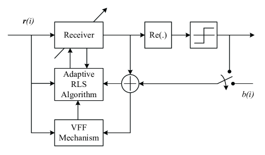
Figure 1: Structure of the adaptive receiver with the variable forgetting factor mechanism

IV Proposed Variable Forgetting Factor Mechanism

In this section, we first introduce the proposed low-complexity CTVFF mechanism that adjusts the forgetting factor of the RLS algorithm that equips the adaptive receiver. Then, we present the computational complexity analysis for the proposed CTVFF mechanism and the existing gradient-based mechanisms.

IV-A Adaptive CTVFF Mechanism

Based on the variable step-size mechanism for least mean square (LMS) algorithms in [28], the motivation for the proposed CTVFF mechanism is that for large estimation errors the adaptive algorithm will employ smaller forgetting factors whereas small estimation errors will result in an increase of the forgetting factor in order to yield smaller misadjustment. Thus, the CTVFF mechanism employs an exponential weighting parameter that controls the quality of the estimation error, and we have devised the following time-averaged expression

$$\gamma(i)=\delta_{1}\gamma(i-1)+\delta_{2}\rho^{2}(i),$$ (16)

where $0<\delta_{1}<1$ and $\delta_{2}>0$, and $\delta_{1}$ is close to $1$ and $\delta_{2}$ is set to be a small value. The quantity $\rho(i)$ denotes the time average estimate related to the correlation of $|b_{k}(i-1)-\mathbf{w}^{H}_{k}(i-1)\mathbf{r}(i-1)|$ and $|b_{k}(i)-\mathbf{w}^{H}_{k}(i)\mathbf{r}(i)|$, which is given by

$$\begin{split}\rho(i)&=\delta_{3}\rho(i-1)+(1-\delta_{3})|b_{k}(i-1)-\mathbf{w}^{H}_{k}(i-1)\mathbf{r}(i-1)||b_{k}(i)-\mathbf{w}^{H}_{k}(i)\mathbf{r}(i)|,\end{split}$$ (17)

where $0<\delta_{3}<1$, and $\delta_{3}$ controls the time average estimate. We set $\delta_{3}$ to be a quantity close to $1$.

The updated component $\rho(i)$ is a small value, and it changes rapidly as the instantaneous value of the correlation between $|b_{k}(i-1)-\mathbf{w}^{H}_{k}(i-1)\mathbf{r}(i-1)|$ and $|b_{k}(i)-\mathbf{w}^{H}_{k}(i)\mathbf{r}(i)|$. The use of $\gamma(i)$ has the potential to provide a suitable indication of the evolution of the error correlation. Thus, unlike the conventional GVFF mechanism we aim to design a simpler mechanism that adjusts the forgetting factor automatically based on $\gamma(i)$. Note that the forgetting factor should vary in an inversely proportional way to the value of the error correlation. We have studied a number of rules and the following expression is a result of several attempts to devise a simple and yet effective mechanism

$$\lambda(i)=\bigg{[}\frac{1}{1+\gamma(i)}\bigg{]}^{\lambda^{+}}_{\lambda^{-}}.$$ (18)

Indeed, the CTVFF mechanism is simple to implement and a detailed analysis of the algorithm is possible under a few assumptions commonly made in the literature. The proposed low-complexity CTVFF mechanism is given by (16), (17) and (18). The value of variable forgetting factor $\lambda(i)$ is close to $1$, and it is controlled by the parameters $\delta_{1}$, $\delta_{2}$ and $\delta_{3}$. We will investigate the sensitivity of the parameters in Section VI. A large prediction error will cause the updated component $\gamma(i)$ to increase, which simultaneously reduces the forgetting factor $\lambda(i)$ and provides a faster tracking. While a small prediction error will result in a decrease in the updated component $\gamma(i)$, thereby the forgetting factor $\lambda(i)$ is increased to yield a smaller misadjustment.

IV-B Computational Complexity

We describe the computational complexity of the proposed CTVFF and the adaptive GVFF, WGVFF and MGVFF mechanisms [21, 25, 27]. Table LABEL:tab:table13 shows the additional computational complexity of the algorithms for multipath channels. We estimate the number of arithmetic operations by considering the number of complex additions and multiplications required by the mechanisms. The CTVFF and MGVFF mechanisms have constant computational complexity for each received symbol while the adaptive GVFF and WGVFF techniques have additional complexity proportional to the length $M$ of the receive filter. An important advantage of the proposed adaptation rule is that it requires only ten operations.

TABLE I: Additional Computational complexity.

	Number of operations per symbol
Algorithm	Multiplications	Additions
CTVFF	$7$	$3$
GVFF [21]	$7M^{2}+4M+2$	$7M^{2}+M$
WGVFF [25]	$7M^{2}+4M+9$	$7M^{2}+M+1$
MGVFF [27]	$29$	$18$

V ANALYSES OF THE PROPOSED ALGORITHMS

In this section, we first show the convergence of the mean weight vector and derive the steady-state MSE expression for the adaptive receiver with the proposed CTVFF mechanism in the case of invariant channels. Then, we give the tracking analysis of the proposed scheme for the scenario of time-varying channels. Finally, the expression for the steady-state mean value of the CTVFF mechanism is derived.

V-A Convergence of the Mean Weight Vector

We show the convergence of the mean weight vector of the proposed algorithm. Firstly, we give two expressions which will be used for the following derivation:

$$\mathbf{k}(i)=\mathbf{R}^{-1}(i)\mathbf{r}(i)$$ (19)

and

$$\lim_{i\rightarrow\infty}\mathbf{R}^{-1}(i)\approx\big{(}1-E[\lambda(\infty)]\big{)}\mathbf{\bar{R}}^{-1}.$$ (20)

The proof of (19) and (20) are shown in the appendix. The relevant description is given in [29]-[31].

Let us recall (9) and assume

$$b_{k}(i)=\mathbf{w}^{H}_{0}\mathbf{r}(i)+\xi_{0}(i),$$ (21)

where $\xi_{0}(i)$ denotes the independent measurement error with zero mean and variance $\sigma^{2}_{0}$, where $\sigma^{2}_{0}=1-A_{k}\mathbf{w}^{H}_{0}\mathbf{C}_{k}\mathbf{h}-A_{k}\mathbf{h}^{H}\mathbf{C}^{H}_{k}\mathbf{w}_{0}+\mathbf{w}^{H}_{0}\mathbf{\bar{R}}\mathbf{w}_{0}$, which is computed by (21). By defining $\mbox{\boldmath$\epsilon$}(i)=\mathbf{w}_{k}(i)-\mathbf{w}_{0}$ and using (9) we have

$$\mbox{\boldmath$\epsilon$}(i)=\mathbf{w}_{k}(i)-\mathbf{w}_{0}=\mathbf{w}_{k}(i-1)-\mathbf{w}_{0}+\mathbf{k}(i)e^{*}(i),$$ (22)

based on (19) we have

$$\begin{split}\mbox{\boldmath$\epsilon$}(i)&=\mbox{\boldmath$\epsilon$}(i-1)+\mathbf{R}^{-1}(i)\mathbf{r}(i)\big{(}b^{*}_{k}(i)-\mathbf{r}^{H}(i)\mathbf{w}_{k}(i-1)\big{)}\\ &=\mbox{\boldmath$\epsilon$}(i-1)+\mathbf{R}^{-1}(i)\mathbf{r}(i)\big{(}\xi^{*}_{0}(i)-\mathbf{r}^{H}(i)\mbox{\boldmath$\epsilon$}(i-1)\big{)}\\ &=\big{(}\mathbf{I}-\mathbf{R}^{-1}(i)\mathbf{r}(i)\mathbf{r}^{H}(i)\big{)}\mbox{\boldmath$\epsilon$}(i-1)+\mathbf{R}^{-1}(i)\mathbf{r}(i)\xi^{*}_{0}(i).\end{split}$$ (23)

When $i\rightarrow\infty$, by substituting (20) into (23) we obtain

$$\begin{split}\mbox{\boldmath$\epsilon$}(i)&=\big{(}\mathbf{I}-\big{(}1-E[\lambda(\infty)]\big{)}\mathbf{\bar{R}}^{-1}\mathbf{r}(i)\mathbf{r}^{H}(i)\big{)}\mbox{\boldmath$\epsilon$}(i-1)+\big{(}1-E[\lambda(\infty)]\big{)}\mathbf{\bar{R}}^{-1}\mathbf{r}(i)\xi^{*}_{0}(i).\end{split}$$ (24)

We note that $1-E[\lambda(\infty)]$ is a small value. According to the direct averaging method described in [21], the solution of the stochastic difference equation (24), operating under the condition of a small parameter $1-E[\lambda(\infty)]$, is close to the solution of another linear stochastic difference equation that is obtained by replacing the matrix $(1-E[\lambda(\infty)])\mathbf{r}(i)\mathbf{r}^{H}(i)$ with its ensemble average $(1-E[\lambda(\infty)])\mathbf{\bar{R}}$. We may write the new expression as follows

$$\begin{split}\mbox{\boldmath$\epsilon$}(i)&\approx\big{(}\mathbf{I}-\big{(}1-E[\lambda(\infty)]\big{)}\mathbf{\bar{R}}^{-1}\mathbf{\bar{R}}\big{)}\mbox{\boldmath$\epsilon$}(i-1)+\big{(}1-E[\lambda(\infty)]\big{)}\mathbf{\bar{R}}^{-1}\mathbf{r}(i)\xi^{*}_{0}(i).\\ &=E[\lambda(\infty)]\mbox{\boldmath$\epsilon$}(i-1)+\big{(}1-E[\lambda(\infty)]\big{)}\mathbf{\bar{R}}^{-1}\mathbf{r}(i)\xi^{*}_{0}(i).\end{split}$$ (25)

By taking the expectation of (25), when $i\rightarrow\infty$, we have

$$E[\mbox{\boldmath$\epsilon$}(i)]\approx E[\lambda(\infty)]E[\mbox{\boldmath$\epsilon$}(i-1)].$$ (26)

Since $0<E[\lambda(\infty)]<1$, the expected weight error converges to zero.

V-B Convergence of MSE

Then, we show the convergence of MSE for the proposed algorithm and give an analytical expression to predict the steady-state MSE.

Based on (25) we have

$$\begin{split}\mbox{\boldmath$\Theta$}(i)&=E[\mbox{\boldmath$\epsilon$}(i)\mbox{\boldmath$\epsilon$}^{H}(i)]\\ &\approx E^{2}[\lambda(\infty)]E[\mbox{\boldmath$\epsilon$}(i-1)\mbox{\boldmath$\epsilon$}^{H}(i-1)]\\ &\quad+\big{(}1-E[\lambda(\infty)]\big{)}^{2}E[\mathbf{\bar{R}}^{-1}\mathbf{r}(i)\xi^{*}_{0}(i)\xi_{0}(i)\mathbf{r}^{H}(i)\mathbf{\bar{R}}^{-1}]\\ &\quad+E[\lambda(\infty)]\big{(}1-E[\lambda(\infty)]\big{)}E[\mathbf{\bar{R}}^{-1}\mathbf{r}(i)\xi^{*}_{0}(i)]E[\mbox{\boldmath$\epsilon$}^{H}(i-1)]\\ &\quad+E[\lambda(\infty)]\big{(}1-E[\lambda(\infty)]\big{)}E[\mbox{\boldmath$\epsilon$}(i-1)]E[\xi_{0}(i)\mathbf{r}^{H}(i)\mathbf{\bar{R}}^{-1}].\end{split}$$ (27)

Note that when $i\rightarrow\infty$, $E[\mbox{\boldmath$\epsilon$}(i-1)]\approx\mathbf{0}$, we have

$$\mbox{\boldmath$\Theta$}(i)\approx E^{2}[\lambda(\infty)]\mbox{\boldmath$\Theta$}(i-1)+\big{(}1-E[\lambda(\infty)]\big{)}^{2}\mathbf{\bar{R}}^{-1}\sigma^{2}_{0}.$$ (28)

Since $0<E^{2}[\lambda(\infty)]<1$, we obtain

$$\mbox{\boldmath$\Theta$}(\infty)\approx\Big{(}\frac{1-E[\lambda(\infty)]}{1+E[\lambda(\infty)]}\Big{)}\mathbf{\bar{R}}^{-1}\sigma^{2}_{0}.$$ (29)

Note that the steady-state MSE is given by

$$\begin{split}\lim_{i\rightarrow\infty}\xi(i)&=\lim_{i\rightarrow\infty}E[|b_{k}(i)-\mathbf{w}^{H}_{k}(i-1)\mathbf{r}(i)|^{2}]\\ &=\lim_{i\rightarrow\infty}(\Xi(i)+1-A_{k}\mathbf{w}^{H}_{0}\mathbf{C}_{k}\mathbf{h}-A_{k}\mathbf{h}^{H}\mathbf{C}^{H}_{k}\mathbf{w}_{0}),\end{split}$$ (30)

and

$$\begin{split}\Xi(i)&=E[(\mbox{\boldmath$\epsilon$}^{H}(i-1)+\mathbf{w}^{H}_{0})\mathbf{r}(i)\mathbf{r}^{H}(i)(\mbox{\boldmath$\epsilon$}(i-1)+\mathbf{w}_{0})]\\ &=\mathbf{w}^{H}_{0}\mathbf{\bar{R}}\mathbf{w}_{0}+{\rm tr}[\mathbf{\bar{R}}\mathbf{\Theta}(i-1)]+E[\mbox{\boldmath$\epsilon$}^{H}(i-1)]E[\mathbf{r}(i)\mathbf{r}^{H}(i)\mathbf{w}_{0}]\\ &\quad+E[\mathbf{w}^{H}_{0}\mathbf{r}(i)\mathbf{r}^{H}(i)]E[\mbox{\boldmath$\epsilon$}(i-1)].\end{split}$$ (31)

When $i\rightarrow\infty$, we have $\Xi(\infty)=\mathbf{w}^{H}_{0}\mathbf{\bar{R}}\mathbf{w}_{0}+{\rm tr}[\mathbf{\bar{R}}\mathbf{\Theta}(\infty)]$. Multiplying (29) by $\mathbf{\bar{R}}$ we have

$${\rm tr}[\mathbf{\bar{R}}\mathbf{\Theta}(\infty)]\approx\Big{(}\frac{1-E[\lambda(\infty)]}{1+E[\lambda(\infty)]}\Big{)}\sigma^{2}_{0}M.$$ (32)

Therefore, the steady-state MSE in (30) can be approximated by the following expression

$$\xi(\infty)\approx\xi_{\rm min}+\Big{(}\frac{1-E[\lambda(\infty)]}{1+E[\lambda(\infty)]}\Big{)}\sigma^{2}_{0}M,$$ (33)

where $\xi_{\rm min}=1-A^{2}_{k}\mathbf{h}^{H}(i)\mathbf{C}^{H}_{k}\mathbf{\bar{R}}^{-1}\mathbf{C}_{k}\mathbf{h}(i)$.

V-C Tracking Analysis

In a nonstationary scenario, the optimum solution takes on a time-varying form. It brings a new task to track the minimum point of the error-performance surface, which is no longer fixed. We investigate the convergence properties of the proposed algorithm in this case. In time-varying channels, the optimum filter coefficients are considered to vary according to the model $\mathbf{w}_{0}(i)=\mathbf{w}_{0}(i-1)+\mathbf{q}(i)$, where $\mathbf{q}(i)$ denotes a random perturbation [21]. We assume that $\mathbf{q}(i)$ is an independently generated sequence with zero mean and positive definite autocorrelation matrix $E[\mathbf{q}(i)\mathbf{q}^{H}(i)]$. This is typical in the context of tracking analyses of adaptive filters [32, 33].

By redefining $\mbox{\boldmath$\epsilon$}(i)=\mathbf{w}_{k}(i)-\mathbf{w}_{0}(i)$ and following the aforementioned approach, we have

$$\begin{split}\mbox{\boldmath$\epsilon$}(i)&=\mathbf{w}_{k}(i)-\mathbf{w}_{0}(i)\\ &=\mathbf{w}_{k}(i-1)-\mathbf{w}_{0}(i-1)-\mathbf{q}(i)+\mathbf{k}(i)e^{*}(i)\\ &=\mbox{\boldmath$\epsilon$}(i-1)-\mathbf{q}(i)+\mathbf{R}^{-1}(i)\mathbf{r}(i)\big{(}\mathbf{r}^{H}(i)\mathbf{w}_{0}(i-1)+\xi^{*}_{0}(i)-\mathbf{r}^{H}(i)\mathbf{w}_{k}(i-1)\big{)}\\ &=\big{(}\mathbf{I}-\mathbf{R}^{-1}(i)\mathbf{r}(i)\mathbf{r}^{H}(i)\big{)}\mbox{\boldmath$\epsilon$}(i-1)+\mathbf{R}^{-1}(i)\mathbf{r}(i)\xi^{*}_{0}(i)-\mathbf{q}(i).\end{split}$$ (34)

Using (20) when $i$ becomes large, we obtain

$$\begin{split}\mbox{\boldmath$\epsilon$}(i)&\approx(\mathbf{I}-(1-E[\lambda(\infty)])\mathbf{\bar{R}}^{-1}\mathbf{r}(i)\mathbf{r}^{H}(i))\mbox{\boldmath$\epsilon$}(i-1)+\big{(}1-E[\lambda(\infty)]\big{)}\mathbf{\bar{R}}^{-1}\mathbf{r}(i)\xi^{*}_{0}(i)-\mathbf{q}(i).\end{split}$$ (35)

Since $1-E[\lambda(\infty)]$ is a small value, we may solve (35) for the weight error vector $\mbox{\boldmath$\epsilon$}(i)$ by employing the direct averaging method [21], which was mentioned previously. We obtain the following expression

$$\begin{split}\mbox{\boldmath$\epsilon$}(i)&\approx E[\lambda(\infty)]\mbox{\boldmath$\epsilon$}(i-1)+\big{(}1-E[\lambda(\infty)]\big{)}\mathbf{\bar{R}}^{-1}\mathbf{r}(i)\xi^{*}_{0}(i)-\mathbf{q}(i).\end{split}$$ (36)

Note that the vector $\mathbf{q}(i)$ is an independent zero mean vector, we have

$$\begin{split}\mbox{\boldmath$\Theta$}(i)&=E[\mbox{\boldmath$\epsilon$}(i)\mbox{\boldmath$\epsilon$}^{H}(i)]\\ &\approx E^{2}[\lambda(\infty)]\mbox{\boldmath$\Theta$}(i-1)+\big{(}1-E[\lambda(\infty)]\big{)}^{2}\mathbf{\bar{R}}^{-1}\sigma^{2}_{0}+E[\mathbf{q}(i)\mathbf{q}^{H}(i)],\end{split}$$ (37)

and when $i$ becomes large, the MSE in a time-varying environment is given by

$$\begin{split}\xi(i)&=E[|b_{k}(i)-\mathbf{w}^{H}_{k}(i-1)\mathbf{r}(i)|^{2}]\\ &=\mathbf{w}^{H}_{0}(i-1)\mathbf{\bar{R}}\mathbf{w}_{0}(i-1)+{\rm tr}[\mathbf{\bar{R}}\mathbf{\Theta}(i)]+1-A_{k}\mathbf{w}^{H}_{0}(i-1)\mathbf{C}_{k}\mathbf{h}-A_{k}\mathbf{h}^{H}\mathbf{C}^{H}_{k}\mathbf{w}_{0}(i-1).\end{split}$$ (38)

By using (37), when $i$ becomes large, we have

$${\rm tr}[\mathbf{\bar{R}}\mbox{\boldmath$\Theta$}(i)]\approx\Big{(}\frac{1-E[\lambda(\infty)]}{1+E[\lambda(\infty)]}\Big{)}\sigma^{2}_{0}M+\frac{{\rm tr}\big{[}\mathbf{\bar{R}}E[\mathbf{q}(i)\mathbf{q}^{H}(i)]\big{]}}{1-E^{2}[\lambda(\infty)]}.$$ (39)

The MSE for a situation in which the adaptive receiver is tracking a channel can be computed by the following expression

$$\xi(\infty)\approx\xi_{\rm min}+\Big{(}\frac{1-E[\lambda(\infty)]}{1+E[\lambda(\infty)]}\Big{)}\sigma^{2}_{0}M+\frac{{\rm tr}\big{[}\mathbf{\bar{R}}E[\mathbf{q}(i)\mathbf{q}^{H}(i)]\big{]}}{1-E^{2}[\lambda(\infty)]}.$$ (40)

Note that we need to compute the quantities $E[\lambda(\infty)]$ and $E[\mathbf{q}(i)\mathbf{q}^{H}(i)]$ to calculate the above expression.

V-D Steady-State Mean Value of the CTVFF Mechanism

In order to derive the expression for the steady-state mean value of the CTVFF mechanism, we first show the convergence and derive the expression for the steady-state statistical property of the updated component $\gamma(i)$.

By recalling (17), the estimate of $\rho(i)$ can be alternatively written as

$$\begin{split}\rho(i)&=(1-\delta_{3})\sum^{i-1}_{l=0}\delta^{l}_{3}|b_{k}(i-l-1)-\mathbf{w}^{H}_{k}(i-l-1)\mathbf{r}(i-l-1)||b_{k}(i-l)-\mathbf{w}^{H}_{k}(i-l)\mathbf{r}(i-l)|\end{split}$$ (41)

and by squaring (41) we have

$$\begin{split}\rho^{2}(i)&=(1-\delta_{3})^{2}\sum^{i-1}_{l=0}\sum^{i-1}_{j=0}\delta^{l}_{3}\delta^{j}_{3}|b_{k}(i-l-1)-\mathbf{w}^{H}_{k}(i-l-1)\mathbf{r}(i-l-1)|\\ &\quad\times|b_{k}(i-j-1)-\mathbf{w}^{H}_{k}(i-j-1)\mathbf{r}(i-j-1)||b_{k}(i-l)-\mathbf{w}^{H}_{k}(i-l)\mathbf{r}(i-l)|\\ &\quad\times|b_{k}(i-j)-\mathbf{w}^{H}_{k}(i-j)\mathbf{r}(i-j)|.\end{split}$$ (42)

When $i\rightarrow\infty$, we assume that $|b_{k}(i-l)-\mathbf{w}^{H}_{k}(i-l)\mathbf{r}(i-l)|$ and $|b_{k}(i-j)-\mathbf{w}^{H}_{k}(i-j)\mathbf{r}(i-j)|$ are uncorrelated, thus, we have $E[|b_{k}(i-l)-\mathbf{w}^{H}_{k}(i-l)\mathbf{r}(i-l)||b_{k}(i-j)-\mathbf{w}^{H}_{k}(i-j)\mathbf{r}(i-j)|]=E[|b_{k}(i-l)-\mathbf{w}^{H}_{k}(i-l)\mathbf{r}(i-l)|]E[|b_{k}(i-j)-\mathbf{w}^{H}_{k}(i-j)\mathbf{r}(i-j)|]\approx 0$, where $\forall j\neq l$. Hence, the expectation of $\rho^{2}(i)$ is given by

$$\begin{split}E[\rho^{2}(i)]&=(1-\delta_{3})^{2}\sum^{i-1}_{l=0}\delta^{2l}_{3}E[|b_{k}(i-l-1)-\mathbf{w}^{H}_{k}(i-l-1)\mathbf{r}(i-l-1)|^{2}]E[|b_{k}(i-l)-\mathbf{w}^{H}_{k}(i-l)\mathbf{r}(i-l)|^{2}].\end{split}$$ (43)

Note that $0<\delta_{3}<1$, by using $\lim_{i\rightarrow\infty}E[|b_{k}(i)-\mathbf{w}^{H}_{k}(i)\mathbf{r}(i)|^{2}]=\xi_{min}$, we obtain

$$E[\rho^{2}(i)]=\frac{(1-\delta_{3})\xi^{2}_{min}}{(1+\delta_{3})}.$$ (44)

Note that $0<\delta_{1}<1$, based on (16) we obtain the steady-state mean for $\gamma(i)$,

$$E[\gamma(\infty)]=\frac{\delta_{2}(1-\delta_{3})\xi^{2}_{min}}{(1-\delta_{1})(1+\delta_{3})}.$$ (45)

From (16) and (17), we can see that the quantity $\gamma(i)$ is a small value, and $\gamma(i)$ varies slowly around its mean value. Thus, when $i\rightarrow\infty$, by using (18) and (45) we assume that the steady-state mean value of the variable forgetting factor for the CTVFF mechanism is given as

$$\begin{split}E[\lambda(\infty)]&\approx\frac{1}{1+E[\gamma(\infty)]}\\ &=\frac{(1-\delta_{1})(1+\delta_{3})}{(1-\delta_{1})(1+\delta_{3})+\delta_{2}(1-\delta_{3})\xi^{2}_{min}}.\end{split}$$ (46)

The above value can be substituted in (33) and (40) to predict the MSE.

VI Simulations

In this section, we first adopt a simulation approach and conduct several experiments in order to verify the effectiveness of the proposed CTVFF mechanism in RLS algorithms applied to interference suppression problems with DS-CDMA systems. Then, we verify the effectiveness of the proposed analytical expressions in (33), (40) and (46) to predict the performance of the adaptive linear receivers in several situations. The DS-CDMA system employs Gold sequences as the spreading codes, and the spreading gain is $N=15$. The sequence of channel coefficients for each path is given by $h_{f}(i)=p_{f}\alpha_{f}(i)(f=0,1,2)$. All channels are normalized so that

$$\sum^{L_{p}-1}_{f=0}p^{2}_{f}=1,$$ (47)

where $\alpha_{f}(i)$ is computed according to the Jakes’ model [2]. For the initial values, we set $\mathbf{R}^{-1}(0)=\mathbf{I}$, $\mathbf{w}_{k}(0)=0.01\times\mathbf{1}$, $\frac{\mathbf{\partial\mathbf{w}_{k}(0)}}{\partial\lambda}=\mathbf{0}$ and $\frac{\mathbf{\partial\mathbf{R}^{-1}(0)}}{\partial\lambda}=\mathbf{I}$, where $\mathbf{1}$ denotes an all-one vector. The parameters of the MGVFF and WGVFF mechanisms are set as [27, 25]. The simulations are averaged over $10000$ runs. We set the power of the desired user $|A_{1}|^{2}=1$.

VI-A Effects of $\delta_{1}$, $\delta_{2}$ and $\delta_{3}$

Fig. 2 shows the effect of $\delta_{3}$ on the proposed CTVFF mechanism. We show the received steady-state signal to interference plus noise ratio (SINR) versus $\delta_{3}$ for different values of $\delta_{1}$ and $\delta_{2}$ under different scenarios. For the first scenario, we consider that the system has six users including two users operating at a power level $3dB$ above and one user operating at a power level $6dB$ above the desired user’s power level. The channel fading rate is $f_{d}T=1\times 10^{-5}$. The channel power profile is given by $p_{0}=0dB$, $p_{1}=-6dB$ and $p_{2}=-10dB$. For the second scenario, the system has ten users which have the same power level. In this case, we consider a static channel, the channel parameters of which are given by $h_{0}=0dB$, $h_{1}=-3dB$ and $h_{2}=-6dB$. In Fig. 2, we can see that the performance does not change too much as the value of $\delta_{3}$ varies for different values of $\delta_{1}$ and $\delta_{2}$. We set $\gamma^{-}=0.98$ and $\gamma^{+}=0.99998$, and use $15dB$ for the input signal to noise ratio (SNR). We tuned $\delta_{3}=0.99$ for the following simulations.

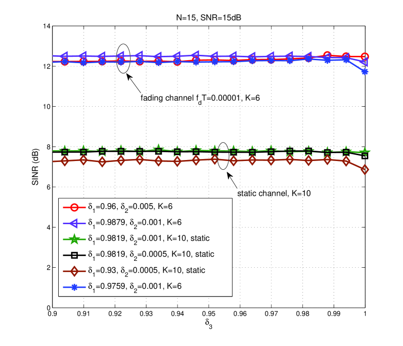
Figure 2: Steady-state SINR versus $\delta_{3}$ for different values of $\delta_{1}$ and $\delta_{2}$. $SNR=15$ dB.

We investigate the effects of $\delta_{1}$ and $\delta_{2}$ on the CTVFF mechanism, we show the received steady-state SINR versus $\delta_{1}$ for $\delta_{2}=0.015,0.005,0.001,0.0005,0.0001$ under different scenarios, where we tuned $\delta_{3}=0.99$. We use $15dB$ for the input SNR, and set $\gamma^{-}=0.98$ and $\gamma^{+}=0.99998$ for the CTVFF mechanism to guarantee the stability. The results shown in Fig. 3 (a) and (b) are based on a static state channel. The time-invariant channel parameters are given by $h_{0}=0dB$, $h_{1}=-3dB$ and $h_{2}=-6dB$. In Fig. 3 (a), the system has six users with the same power level. In Fig. 3 (b), the system has ten users with the same power level. It is observed that, firstly, the optimum choice of the pair $(\delta_{1},\delta_{2})$ is not unique, for each value of $\delta_{2}$ we can find a relevant $\delta_{1}$ to have the best performance. Secondly, with the increasing of $\delta_{2}$ the performance becomes less sensitive to $\delta_{1}$. Moreover, when $\delta_{2}$ increases to $0.005$, the performance becomes insensitive to $\delta_{1}$. From the results, we can obtain that $\delta_{1}=0.9819$ and $\delta_{2}=0.005$ are one of the best choices for the scenario in Fig. 3 (a) and $\delta_{1}=0.9879$ and $\delta_{2}=0.001$ are one of the best choices for both scenarios, which shows that it is possible for us to find a pair $(\delta_{1},\delta_{2})$ that works well for different scenarios.

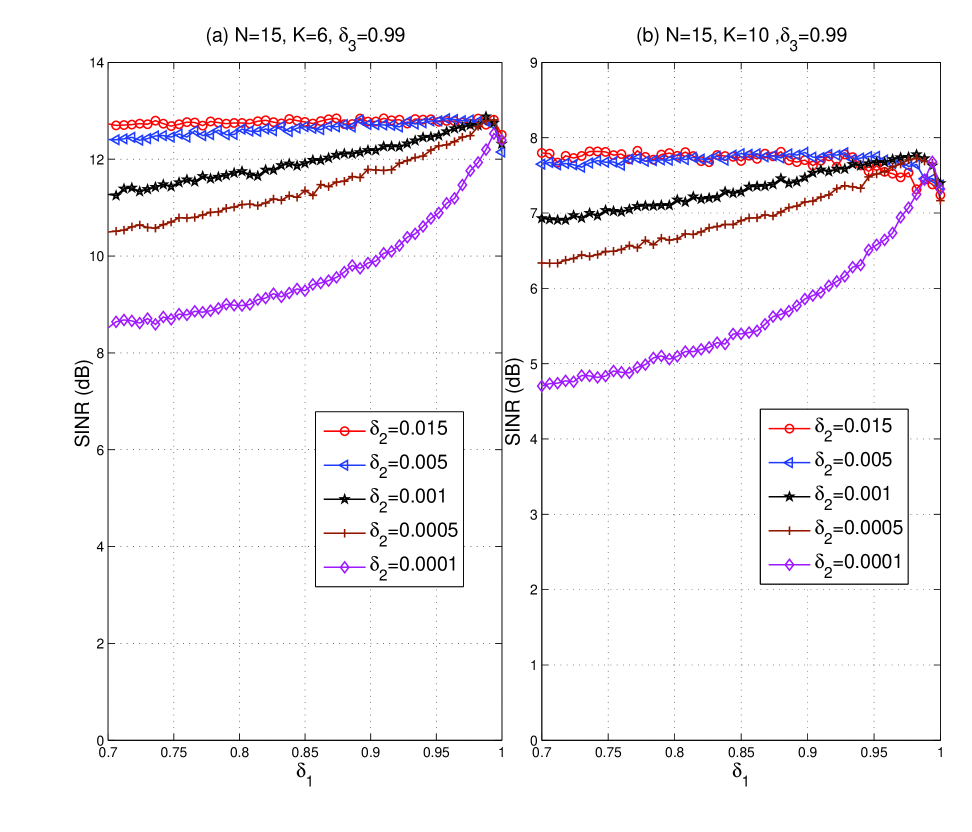
Figure 3: Steady-state SINR versus $\delta_{1}$ for different values of $\delta_{2}$. (a) $K=6$, with equal power level interferers, (b) $K=10$, with equal power level interferers. $\delta_{3}=0.99$, static channel.

The results in Fig. 4 (a) and (b) show the steady-state SINR versus $\delta_{1}$ for different values of $\delta_{2}$ based on the channel with $f_{d}T=0.00001$. The channel has a power profile given by $p_{0}=0dB$, $p_{1}=-6dB$ and $p_{2}=-10dB$. We tuned $\delta_{3}=0.99$. In Fig. 4 (a), the system includes six users including two users operating at a power level $3dB$ above and one user operating at a power level $6dB$ above the desired user’s power level. In Fig. 4 (b), the system has ten users including four users operating at a power level $3dB$ above and two users operating at a power level $6dB$ above the desired user’s power level. We can see that the previous findings on effects of $\delta_{1}$ and $\delta_{2}$ still hold for the experiments. In particular, in Fig. 4 (a), when $\delta_{2}$ increases to $0.015$, the performance becomes insensitive to $\delta_{1}$. In this case, we found that $\delta_{1}=0.934$ and $\delta_{2}=0.005$ are one of the best choices for both scenarios. In the following experiments, for a given scenario we first choose the optimum parameters, and then fix them through the simulations. In practice, these optimized values should be obtained by experimentation for a given range of values or a specific operating point, and stored at the receiver.

Figure 4: Steady-state SINR versus $\delta_{1}$ for different values of $\delta_{2}$. (a) $K=6$, with two $3$dB and one $6$dB high power level interferers, (b) $K=10$, with four $3$dB and two $6$dB high power level interferers. $f_{d}T=0.00001$, $\delta_{3}=0.99$.

VI-B Performance of the Proposed Algorithm

We first choose the received SINR as the performance index to evaluate the convergence performance in nonstationary scenarios. In this simulation, we assess the SINR performance of the proposed CTVFF mechanism, the adaptive GVFF mechanism, the MGVFF mechanism, the WGVFF mechanism, the fixed forgetting factor mechanism and the adaptive SG receiver. The results shown in Fig. 5 illustrate that the performance in terms of SINR of the analyzed algorithms in a nonstationary scenario. The channel has a power profile given by $p_{0}=0dB$, $p_{1}=-6dB$ and $p_{2}=-10dB$. The system starts with six users including two users operating at a power level $3$ dB above and one user operating at a power level $6$ dB above the desired user’s power level. At $1000$ symbols, four interferers including two users operating at a power level $3$ dB above and one user operating at a power level $6$ dB above the desired user’s power level enter the system. The normalized Doppler frequency is $f_{d}T=1\times 10^{-5}$. From Fig. 5, we can see that the proposed CTVFF mechanism with the adaptive receiver achieves the best performance, followed by the WGVFF mechanism with the RLS receiver and the GVFF mechanism with the RLS receiver. The MGVFF mechanism does not work well in the nonstationary scenario of multipath fading channels. The algorithms process $250$ symbols in the TR mode. For the simulation, we tuned the forgetting factor $\lambda=0.997$ for the fixed forgetting factor scheme. For the GVFF mechanism, we tuned $\lambda^{-}=0.992$, $\lambda^{+}=0.99998$, $\lambda(0)=0.998$ and $\mu=0.0025$. For the proposed CTVFF mechanism, we tuned $\lambda^{-}=0.98$, $\lambda^{+}=0.99998$, $\delta_{1}=0.934$, $\delta_{2}=0.005$, $\delta_{3}=0.99$, $\gamma(0)=0$ and $\rho(0)=0$.

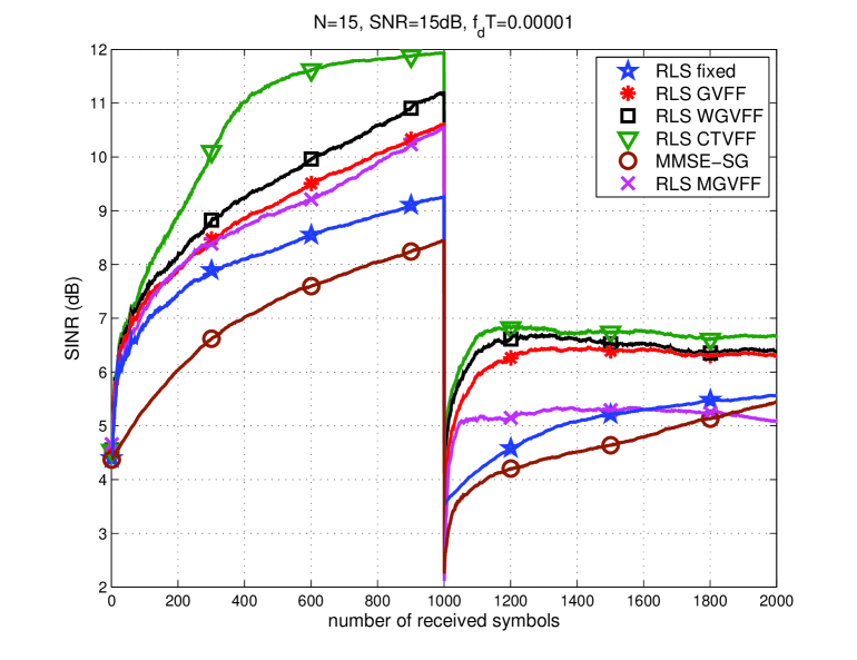
Figure 5: SINR performance in nonstationary environment of multipath fading channels. SNR$=15$dB. $f_{d}T=0.00001$.

The result shown in Fig. 6 illustrates the variation of the forgetting factor value of the proposed CTVFF mechanism versus number of received symbols in the experiment of Fig. 5. We can see that the forgetting factor value becomes small at the first several iterations due to the large prediction error and it increases gradually until the system converges. At $1000$ symbols, when the new interferers enter the system, the forgetting factor will be recomputed.

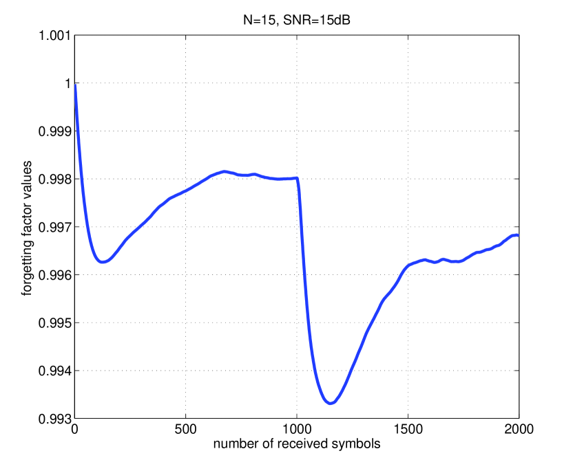
Figure 6: Forgetting factor variation of the proposed CTVFF scheme in nonstationary scenarios. SNR$=15$dB, $f_{d}T=1\times 10^{-5}$.

In Fig. 7, we depict the SINR performance of the analyzed algorithms in a different nonstationary scenario. The channel has a power profile given by $p_{0}=0dB$, $p_{1}=-3dB$ and $p_{2}=-6dB$. The normalized Doppler frequency is $f_{d}T=1\times 10^{-4}$. The system starts with eight users including three users operating at a power level $3dB$ above and one user operating at a power level $6dB$ above the desired user’s power level. At $1000$ symbols, four interferers including two users operating at a power level $3dB$ above the desired user’s power level enter the system. From the results, we can see that the adaptive receiver with the CTVFF mechanism works well and still outperforms the conventional techniques. For the proposed CTVFF mechanism, we maintained the parameters in the simulation of Fig. 5. We tuned the forgetting factor $\lambda=0.995$ for the fixed forgetting factor scheme. For the GVFF mechanism, we tuned $\lambda^{-}=0.992$, $\lambda^{+}=0.99998$ and $\mu=0.0035$.

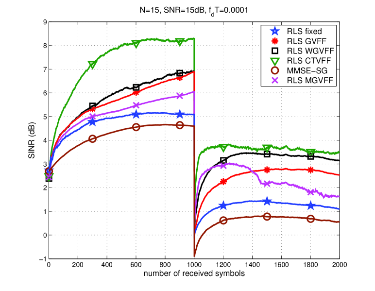
Figure 7: SINR performance in nonstationary environment of multipath fading channels. SNR$=15$dB. $f_{d}T=0.0001$.

We examine the SINR performance of the CTVFF mechanism in a static environment. We compare the CTVFF mechanism with the adaptive GVFF mechanism, the MGVFF mechanism, the WGVFF mechanism, the fixed forgetting factor mechanism and the adaptive SG receiver. Fig. 8 illustrates the SINR performance versus the number of received symbols for a static environment, where the time-invariant channel parameters are given by $h_{0}=0dB$, $h_{1}=-3dB$ and $h_{2}=-6dB$. The system includes six users which have equal power level. The results show that the proposed CTVFF mechanism works well in a static environment, and it outperforms the other conventional schemes. For the simulation, we tuned the forgetting factor $\lambda=0.9995$ for the fixed forgetting factor scheme. For the GVFF mechanism, we tuned $\lambda^{-}=0.992$, $\lambda^{+}=0.99998$, $\lambda(0)=0.998$ and $\mu=0.006$. For the proposed CTVFF mechanism, we tuned $\lambda^{-}=0.98$, $\lambda^{+}=0.99998$, $\delta_{1}=0.9879$, $\delta_{2}=0.001$ and $\delta_{3}=0.99$.

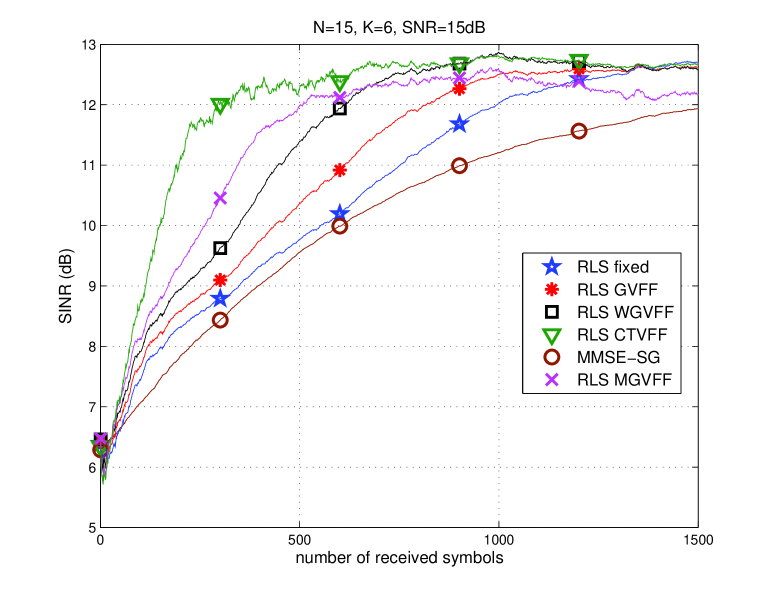
Figure 8: SINR performance in a static environment. SNR$=15$dB. $K=6$.

We show the bit error rate (BER) performance of the following algorithms as the fading rate of the channel varies, i.e., the RLS receiver with the proposed CTVFF mechanism, the RLS receiver with the GVFF mechanism, the RLS receiver with the WGVFF mechanism, the RLS receiver with the fixed forgetting factor mechanism and the adaptive SG receiver. In this experiment, the values of the forgetting factors for the algorithms which employ fixed forgetting factors are optimized, and we tuned suitable forgetting factors for each value of $f_{d}T$. The channel has a power profile given by $p_{0}=0dB$, $p_{1}=-6dB$ and $p_{2}=-10dB$. In Fig. 9, we can see that, as the fading rate increases, the performance gets worse, and our proposed CTVFF scheme outperforms the existing schemes, which shows the ability of the RLS receiver with the CTVFF mechanism to deal with channel uncertainties. For the GVFF mechanism, we tuned $\lambda^{-}=0.993$, $\lambda^{+}=0.99998$ and $\mu=0.003$. For the proposed CTVFF mechanism, we tuned $\lambda^{-}=0.98$, $\lambda^{+}=0.99998$, $\delta_{1}=0.988$, $\delta_{2}=0.001$ and $\delta_{3}=0.99$.

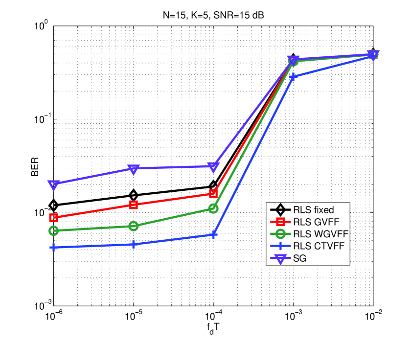
Figure 9: BER performance versus the (cycles/symbol) in multipath fading channels. We use SNR$=15$dB, K$=5$, $1500$ symbols are transmitted and $250$ symbols in TR.

Fig. 10 (a) and (b) illustrate the BER performance of the desired user versus SNR and number of users $K$, respectively, where we set $f_{d}T=1\times 10^{-4}$. We can see that the best performance is achieved by the adaptive receiver with the CTVFF mechanism, followed by the RLS receiver with the WGVFF mechanism, the RLS receiver with the GVFF mechanism, the RLS receiver with the fixed forgetting factor mechanism, the adaptive SG receiver and the conventional Rake receiver. In particular, the adaptive receiver with the CTVFF mechanism can save up to over $4$dB and support up to two more users in comparison with the receiver with the WGVFF mechanism, at the BER level of $10^{-2}$. $1500$ symbols are transmitted and $250$ symbols are used in TR.

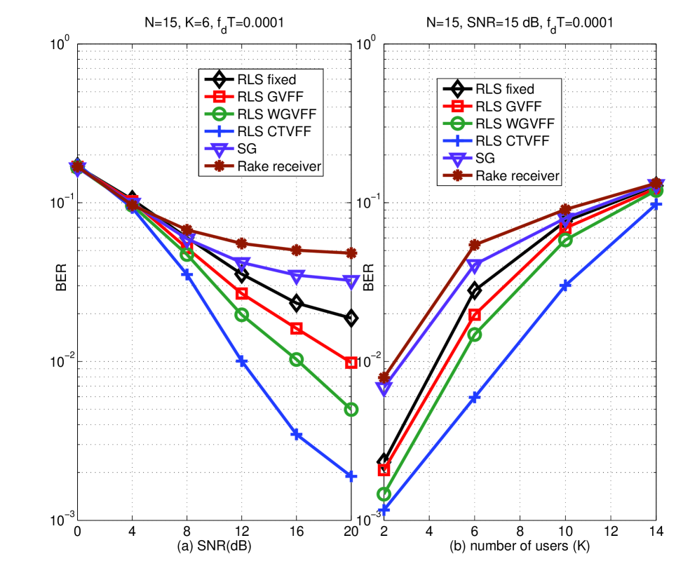
Figure 10: SINR performance versus (a) SNR and (b) the number of users (K) in multipath time varying channels, $f_{d}T=0.0001$.

VI-C Convergence and Tracking Analyses

Then, we examine the convergence and tracking analyses of the proposed CTVFF mechanism with the RLS receiver. The steady-state MSE between the desired and the estimated symbol obtained through simulation is compared with the steady-state MSE computed via the expressions derived in Section V. We verify the analytical results (33) and (46) to predict the steady-state MSE in time-invariant channels and the analytical results (40) and (46) to predict the steady-state MSE in time-varying fading channels. In this simulation, we assume that four users having the same power level operate in the system. The channel has a power profile given by $p_{0}=0dB$, $p_{1}=-6dB$ and $p_{2}=-10dB$. We employ $\delta_{1}=0.99$, $\delta_{2}=0.35\times 10^{-2}$ and $\delta_{3}=0.995$ for the case of invariant channels, and employ $\delta_{1}=0.99$, $\delta_{2}=0.4\times 10^{-3}$ and $\delta_{3}=0.99$ for the case of time-varying fading channels, where $f_{d}T=1\times 10^{-5}$. $250$ symbols are used in TR. The quantity of $E[\mathbf{q}(i)\mathbf{q}^{H}(i)]$ is estimated by using the average over $10000$ independent experiments, namely, $\big{(}\sum^{N_{e}}_{i=1}\mathbf{q}(i)\mathbf{q}^{H}(i)\big{)}/N_{e}$, where $N_{e}=10000$ and $\mathbf{q}(i)=\mathbf{w}_{0}(i)-\mathbf{w}_{0}(i-1)$. By comparing the curves in Fig. 11, it can be seen that as the number of received symbols increases and the simulated MSE values converge to the analytical results, showing the usefulness of our analyses and assumptions.

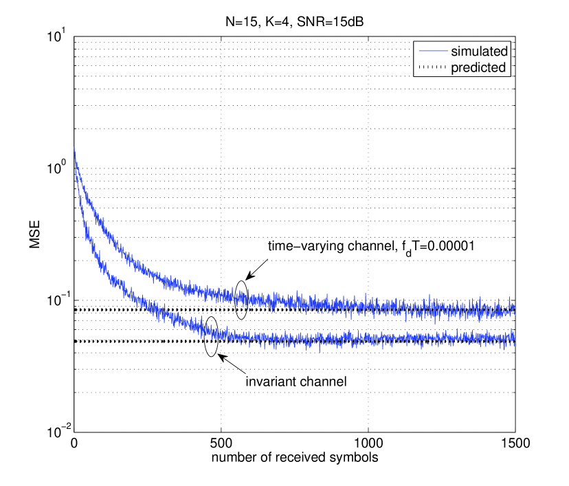
Figure 11: Analytical MSE versus simulated performance for convergence and tracking analyses of the proposed CTVFF scheme. $250$ symbols in TR.

Fig. 12 shows the effect that the desired user’s SNR has on the MSE, and a comparison between the steady-state analysis and simulation results. We assume that four users operate with the same power level in the system. We can see that the simulation and analysis results agree well with each other. $1500$ symbols are transmitted and $250$ symbols are used in TR. For the time-varying fading channel, we use $f_{d}T=1\times 10^{-5}$.

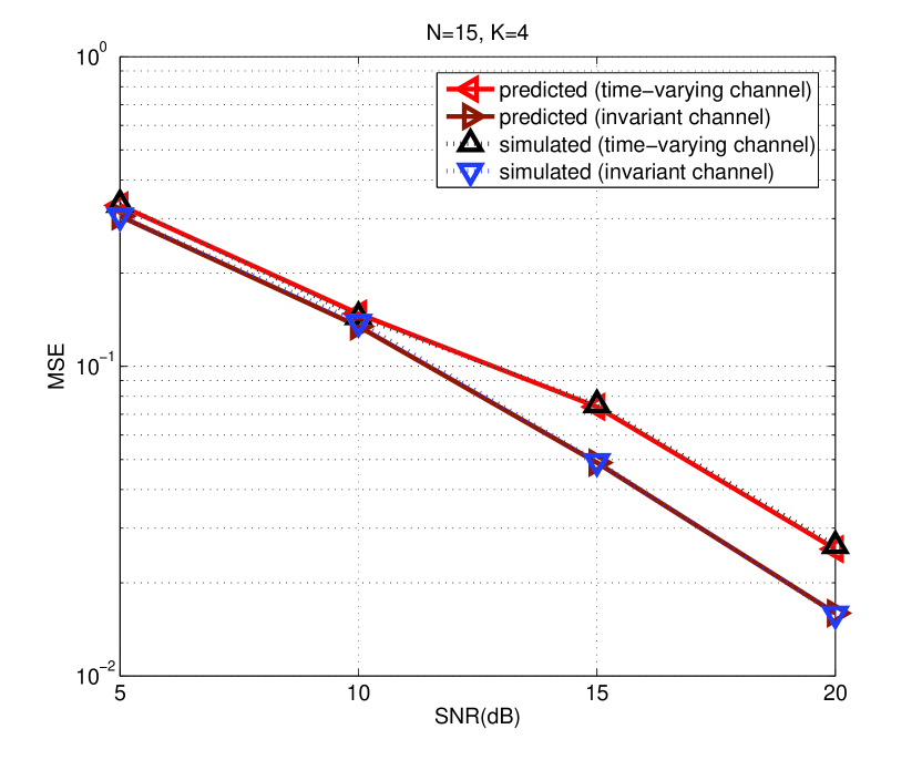
Figure 12: Analytical steady-state MSE versus simulated performance for the proposed CTVFF scheme in time-invariant and time-varying fading channels. $1500$ symbols are transmitted, $250$ symbols in TR.

VII Conclusion

In this paper, we proposed a low-complexity variable forgetting factor mechanism for estimating the parameters of CDMA multiuser detector that operate with RLS algorithms. We compared the computational complexity of the new algorithm with the existing gradient-based methods and further investigated the convergence and tracking analyses of the proposed CTVFF scheme. We also derived expressions to predict the steady-state MSE of the adaptive RLS algorithm with the CTVFF mechanism. The simulation results verify the analytical results and show that the proposed scheme significantly outperforms existing algorithms and supports systems with higher loads. We remark that our proposed algorithm also can be extended to take into account other types of applications.

-A Proof of (19)

By multiplying $\mathbf{r}(i)$ on both sides of (12) we have

$$\begin{split}\mathbf{R}^{-1}(i)\mathbf{r}(i)&=\lambda^{-1}(i)\mathbf{R}^{-1}(i-1)\mathbf{r}(i)-\lambda^{-1}(i)\mathbf{k}(i)\mathbf{r}^{H}(i)\mathbf{R}^{-1}(i-1)\mathbf{r}(i).\end{split}$$ (48)

Rewrite (10) as

$$\begin{split}\mathbf{k}(i)&=\lambda^{-1}(i)\mathbf{R}^{-1}_{k}(i-1)\mathbf{r}(i)-\lambda^{-1}(i)\mathbf{k}(i)\mathbf{r}^{H}(i)\mathbf{R}^{-1}(i-1)\mathbf{r}(i).\end{split}$$ (49)

Based on (48) and (49) we have (19).

-B Derivation of (20)

We note that

$$\begin{split}\mathbf{R}(i)&=\lambda(i)\mathbf{R}(i-1)+\mathbf{r}(i)\mathbf{r}^{H}(i)\\ &=\mathbf{r}(i)\mathbf{r}^{H}(i)+\lambda(i)\mathbf{r}(i-1)\mathbf{r}^{H}(i-1)+\lambda(i)\lambda(i-1)\mathbf{r}(i-2)\mathbf{r}^{H}(i-2)\\ &\quad+\cdots+\lambda(i)\lambda(i-1)\cdots\lambda(2)\mathbf{r}(1)\mathbf{r}^{H}(1)+\lambda(i)\lambda(i-1)\cdots\lambda(2)\lambda(1)\mathbf{r}(0)\mathbf{r}^{H}(0).\end{split}$$ (50)

For large $i$, based on (16), (17) and (18), we assume that there exists a number $N_{i}>0$, when $i\geq N_{i}$, for which we have that the forgetting factor $\lambda(i)$ varies slowly around its mean value and $E[\lambda(N_{i})]\approx E[\lambda(N_{i}+1)]\approx\cdots\approx E[\lambda(i)]\approx E[\lambda(\infty)]$.

By taking the expectation of (50) we obtain

$$\begin{split}E[\mathbf{R}(i)]&\approx E[1+\lambda(i)+\lambda(i)\lambda(i-1)+\cdots+\lambda(i)\lambda(i-1)\cdots\lambda(N_{i})]E[\mathbf{r}(i)\mathbf{r}^{H}(i)]\\ &\quad+E[\lambda(i)\lambda(i-1)\cdots\lambda(N_{i})]E[\lambda(N_{i}-1)\mathbf{r}(N_{i}-2)\mathbf{r}^{H}(N_{i}-2)+\cdots\\ &\quad+\lambda(N_{i}-1)\lambda(N_{i}-2)\cdots\lambda(2)\lambda(1)\mathbf{r}(0)\mathbf{r}^{H}(0)]\\ &\approx\big{(}1+E[\lambda(i)]+E^{2}[\lambda(i)]+\cdots+E^{i-N_{i}+1}[\lambda(i)])E[\mathbf{r}(i)\mathbf{r}^{H}(i)]+E^{i-N_{i}+1}[\lambda(i)]\mbox{\boldmath$\Lambda$},\end{split}$$ (51)

where the matrix $\mbox{\boldmath$\Lambda$}=E[\lambda(N_{i}-1)\mathbf{r}(N_{i}-2)\mathbf{r}^{H}(N_{i}-2)+\cdots+\lambda(N_{i}-1)\lambda(N_{i}-2)\cdots\lambda(2)\lambda(1)\mathbf{r}(0)\mathbf{r}^{H}(0)]$ is determinate. Note that $0<E[\lambda(i)]<1$, when $i\rightarrow\infty$, we obtain

$$E[\mathbf{R}(i)]\approx\frac{1}{1-E[\lambda(\infty)]}E[\mathbf{r}(i)\mathbf{r}^{H}(i)].$$ (52)

Note that, when $i\rightarrow\infty$, $\mathbf{R}(i)$ and $\mathbf{R}^{-1}(i)$ converge. Thus, we assume $\lim_{i\rightarrow\infty}\mathbf{R}^{-1}(i)\approx\lim_{i\rightarrow\infty}E[\mathbf{R}^{-1}(i)]\approx\lim_{i\rightarrow\infty}E^{-1}[\mathbf{R}(i)]$. Finally, we obtain (20).

References

- [1] D. Tse and P. Viswanath, Fundamentals of Wireless Communication, Cambridge University Press, 2005.
- [2] T. S. Rappaport, Wireless Communications, Prentice-Hall, Englewood Cliffs, NJ, 1996.
- [3] M. L. Honig and H. V. Poor, “Adaptive interference suppression,” Wireless Communications: Signal Processing Perspectives. Englewood Cliffs, NJ: Prentice-Hall, 1998, ch. 2, pp. 64-128.
- [4] C. Komninakis, C. Fragouli, A. H. Sayed and R. D. Wesel, “Multi-input multi-output fading channel tracking and equalization using kalman estimation,” IEEE Trans. Signal Process., vol. 50, no. 5, pp. 1065-1076, May 2002.
- [5] A. Rontogiannis, V. Kekatos, and K. Berberidis, “A square-root adaptive V-BLAST algorithm for fast time-varying MIMO channels,” IEEE Signal Process. Lett., vol. 13, no. 5, pp. 265-268, May 2006.
- [6] J. H. Choi, H. Y. Yu, Y. H. Lee, “Adaptive MIMO decision feedback equalization for receivers with time-varying channels,” IEEE Trans. Signal Process., vol. 53, no. 11, pp. 4295-4303, Nov. 2005.
- [7] R. C. de Lamare, and R. Sampaio-Neto, “Adaptive reduced-rank equalization algorithms based on alternating optimization design techniques for MIMO systems,” IEEE Trans. Veh. Technol., vol.60, no.6, pp. 2482-2494, July 2011.
- [8] G. L. Stuber, J. R. Barry, S. W. MacLaughlin, Y. Li, M. A. Ingram and T. G. Pratt, “Broadband MIMO-OFDM wireless communications”, Proceedings of the IEEE, vol. 92, no. 2, pp. 271-294, Feb 2004.
- [9] S. Verdu, Multiuser Detection, Cambridge, U.K., 1998.
- [10] G. Woodward, R. Ratasuk, M. L. Honig, and P. B. Rapajic, “Minimum mean-squared error multiuser decision-feedback detectors for DS-CDMA,” IEEE Trans. Commun., vol.50, no. 12, pp. 2104-2112, Dec. 2002.
- [11] R. C. de Lamare, R. Sampaio-Neto, “Adaptive MBER decision feedback multiuser receivers in frequency selective fading channels”, in IEEE Communications Letters, vol. 7, no. 2, Feb. 2003, pp. 73 - 75.
- [12] Y. Cai, R. C. de Lamare and R. Fa, “Switched interleaving techniques with limited feedback for interference mitigation in DS-CDMA systems,” IEEE Trans. Commun., vol. 59, no. 7, pp. 1946-1956, Jul. 2011.
- [13] R. C. de Lamare, R. Sampaio-Neto, and A. Hjorungnes, “Joint iterative interference cancellation and parameter estimation for CDMA systems,” IEEE Commun. Lett., vol. 11, no. 12, pp. 916-918, Dec. 2007.
- [14] R. C. de Lamare and R. Sampaio-Neto,“Minimum mean-squared error iterative successive parallel arbitrated decision feedback detectors for DS-CDMA systems,” IEEE Trans. Commun., vol.56, no. 5, pp. 778-789, May 2008.
- [15] R. C. de Lamare and P. S. R. Diniz, “Set-membership adaptive algorithms based on time-varying error bounds for CDMA interference suppression,” IEEE Trans. Vehicular Technology, vol. 58, pp. 644-654, Feb. 2009.
- [16] R. C. de Lamare and R. Sampaio-Neto, “Adaptive reduced-rank processing based on joint and iterative interpolation, decimation, and filtering,” IEEE Trans. Signal Process., vol. 57, no. 7, Jul. 2009, pp. 2503-2514.
- [17] R. C. de Lamare and R. Sampaio-Neto, “Reduced-rank space-time adaptive interference suppression with joint iterative least squares algorithms for spread-spectrum systems,” IEEE Trans. Veh. Technol., vol. 59, no. 3, Mar. 2010, pp. 1217-1228.
- [18] R. C. de Lamare, M. Haardt and R. Sampaio-Neto, “Blind adaptive constrained reduced-rank parameter estimation based on constant modulus design for CDMA interference suppression,” IEEE Trans. Signal Process. vol. 56, no. 6, pp. 2470-2482, Jun. 2008.
- [19] R. C. de Lamare and R. Sampaio-Neto, “Blind adaptive MIMO receivers for space-time block-coded DS-CDMA systems in multipath channels using the constant modulus criterion,” IEEE Trans. Communications, vol. 58, pp. 21-27, Jan. 2010.
- [20] R.C. de Lamare, R. Sampaio-Neto and M. Haardt, ”Blind Adaptive Constrained Constant-Modulus Reduced-Rank Interference Suppression Algorithms Based on Interpolation and Switched Decimation,” IEEE Trans. on Signal Processing, vol.59, no.2, pp.681-695, Feb. 2011.
- [21] S. Haykin, Adaptive Filter Theory, 4th ed. Englewood Cliffs, NJ: Prentice-Hall, 2002.
- [22] P. Yuvapoositanon and J. Chambers, “An adaptive step-size code constrained minimum output energy receiver for nonstationary CDMA channels,” Proc. IEEE Int. Conf. Acoust. Speech, Signal Process., Apr. 2003, vol. 4, pp. 465-468.
- [23] D. J. Park and B. E. Jun, “Self-perturbing RLS algorithm with fast tracking capability,” Elect. Lett., vol. 28, pp. 558-559, Mar. 1992.
- [24] S. Song, J. Lim, S. Baek, and K. Sung, “Gauss Newton variable forgetting factor recursive least squares for time varying parameter tracking,” Elect. Lett., vol. 36, no. 11, pp. 988-990, May 2000.
- [25] S. Song, J. Lim, S. Baek, and K. Sung, “Variable forgetting factor linear least squares algorithm for frequency selective fading channel estimation,” IEEE Trans. Veh. Technol., vol. 51, no. 3, pp. 613-616, May 2002.
- [26] C. F. So and S. H. Leung, “Variable forgetting factor RLS algorithm based on dynamic equation of gradient of mean square error,” Elect. Lett., vol. 37, no. 3, pp. 202-203, Feb. 2001.
- [27] S. H. Leung and C. F. So, “Gradient-based variable forgetting factor RLS algorithm in time-varying environments,” IEEE Trans. Signal Process., vol. 53, no. 8, pp. 3141-3150, Aug. 2005.
- [28] R. Kwong and E. Johnston, “A variable step size LMS algorithm,” IEEE Trans. Signal Process., vol. 40, no. 7, pp. 1633-1642, Jul. 1992.
- [29] T. Adali and S. H. Ardalan, “On the effect of input signal correlation on weight misadjustment in the RLS algorithm,” IEEE Trans. Signal Process., vol. 43, no. 4, pp. 988-991, Apr. 1995.
- [30] E. Eleftheriou and D. D. Falconer, “Tracking properties and steady-state performance of RLS adaptive filter algorithms,” IEEE Trans. Acoust., Speech, Signal Process., vol. ASSP-34, pp. 1097-1109, Oct. 1986.
- [31] O. D. Macchi and N. J. Bershad, “Adaptive recovery of a chirped sinusoid in noise–Part I: Performance of the RLS algorithm,” IEEE Trans. Signal Process., vol. 39, no. 4, pp. 583-594, Mar. 1991.
- [32] E. Eweda, “Comparison of RLS, LMS, and sign algorithms for tracking randomly time-varying channels,” IEEE Trans. Signal Process., vol. 42, pp. 2937-2944, Nov. 1994.
- [33] B. Widrow and S. D. Stearns, Adaptive Signal Processing, Englewood Cliffs, NJ: Prentice-Hall, 1985.