Queue-Based Random-Access Algorithms:
Fluid Limits and Stability Issues

Abstract

We use fluid limits to explore the (in)stability properties of wireless networks with queue-based random-access algorithms. Queue-based random-access schemes are simple and inherently distributed in nature, yet provide the capability to match the optimal throughput performance of centralized scheduling mechanisms in a wide range of scenarios. Unfortunately, the type of activation rules for which throughput optimality has been established, may result in excessive queue lengths and delays. The use of more aggressive/persistent access schemes can improve the delay performance, but does not offer any universal maximum-stability guarantees.

In order to gain qualitative insight and investigate the (in)stability properties of more aggressive/persistent activation rules, we examine fluid limits where the dynamics are scaled in space and time. In some situations, the fluid limits have smooth deterministic features and maximum stability is maintained, while in other scenarios they exhibit random oscillatory characteristics, giving rise to major technical challenges. In the latter regime, more aggressive access schemes continue to provide maximum stability in some networks, but may cause instability in others. Simulation experiments are conducted to illustrate and validate the analytical results.

I Introduction

Emerging wireless mesh networks typically lack any centralized access control entity, and instead vitally rely on the individual nodes to operate autonomously and to efficiently share the medium in a distributed fashion. This requires the nodes to schedule their individual transmissions and decide on the use of a shared medium based on knowledge that is locally available or only involves limited exchange of information. A popular mechanism for distributed medium access control is provided by the so-called Carrier-Sense Multiple-Access (CSMA) protocol. In the CSMA protocol each node attempts to access the medium after a certain back-off time, but nodes that sense activity of interfering nodes freeze their back-off timer until the medium is sensed idle. While the CSMA protocol is fairly easy to understand at a local level, the interaction among interfering nodes gives rise to quite intricate behavior and complex throughput characteristics on a macroscopic scale. In recent years relatively parsimonious models have emerged that provide a useful tool in evaluating the throughput characteristics of CSMA-like networks, see for instance [3, 8, 9, 39]. Experimental results in Liew et al. [23] demonstrate that these models, while idealized, provide throughput estimates that match remarkably well with measurements in actual systems.

Despite their asynchronous and distributed nature, CSMA-like algorithms have been shown to offer the remarkable capability of achieving the full capacity region and thus match the optimal throughput performance of centralized scheduling mechanisms operating in slotted time [19, 20, 24]. More specifically, any throughput vector in the interior of the convex hull associated with the independent sets in the underlying interference graph can be achieved through suitable back-off rates and/or transmission lengths. Based on this observation, various ingenious algorithms have been developed for finding the back-off rates that yield a particular target throughput vector or that optimize a certain concave throughput utility function in scenarios with saturated buffers [19, 20, 26]. In the same spirit, several effective approaches have been devised for adapting the transmission lengths based on queue length information, and been shown to guarantee maximum stability [18, 29, 34, 35].

Roughly speaking, the maximum-stability guarantees were established under the condition that the activity factors of the various nodes behave as logarithmic functions of the queue lengths. Unfortunately, such activity factors can induce excessive queue lengths and delays, which has triggered a strong interest in developing approaches for improving the delay performance [16, 22, 25, 28, 33]. Motivated by this issue, Ghaderi & Srikant [15] recently showed that it is in fact sufficient for the logarithms of the activity factors to behave as logarithmic functions of the queue lengths, divided by an arbitrarily slowly increasing, unbounded function. These results indicate that the maximum-stability guarantees are preserved for activity functions that are essentially linear for all practical values of the queue lengths, although asymptotically the activity rate must grow slower than any positive power of the queue length. A careful inspection reveals that the proof arguments leave little room to weaken the stated growth condition. Since the growth condition is only a sufficient one, however, it is not clear to what extent it is actually a strict requirement for maximum stability to be maintained.

In the present paper we explore the scope for using more aggressive activity functions in order to improve the delay performance while preserving the maximum-stability guarantees. Since the proof methods of [15, 18, 29, 34, 35] do not easily extend to more aggressive activity functions, we will instead adopt fluid limits where the dynamics of the system are scaled in both space and time. Fluid limits may be interpreted as first-order approximations of the original stochastic process, and provide valuable qualitative insight and a powerful approach for establishing (in)stability properties [5, 6, 7, 27].

As observed in [4], qualitatively different types of fluid limits can arise, depending on the structure of the interference graph, in conjunction with the functional shape of the activity factors. For sufficiently tame activity functions as in [15, 29, 34, 35], ‘fast mixing’ is guaranteed, where the activity process evolves on a much faster time scale than the scaled queue lengths. Qualitatively similar fluid limits can arise for more aggressive activity functions as well, provided the topology is benign in a certain sense, which implies that the maximum-stability guarantees are preserved in those cases. In different regimes, however, aggressive activity functions can cause ‘sluggish mixing’, where the activity process evolves on a much slower time scale than the scaled queue lengths, yielding oscillatory fluid limits that follow random trajectories. It is highly unusual for such random dynamics to occur, as in queueing networks typically the random characteristics vanish and deterministic limits emerge on the fluid scale. A few exceptions are known for various polling-type models as considered in [13, 21, 14].

The random nature of the fluid limits gives rise to several complications in the convergence proofs that are not commonly encountered. Since the random-access networks that we consider are fundamentally different from the polling type-models in the above-mentioned references, the fluid limits are qualitatively different as well, and require a substantially different approach to establish convergence. Specifically, we develop an approach based on stopping time sequences to deal with the switching probabilities governing the sample paths of the fluid limit process. While these proof arguments are developed in the context of random-access networks, several key components extend far beyond the scope of the present problem. Hence, we believe that the proof constructs are of broader methodological value in handling random fluid limits and of potential use in establishing both stability and instability results for a wider range of models. For example, the methodology that we develop could be easily applied to prove the stability results for the random capture scheme as conjectured in work of Feuillet et al. [12].

The possible oscillatory behavior of the fluid limit itself does not necessarily imply that the system is unstable, and in some situations maximum stability is in fact maintained. In other scenarios, however, the fluid limit reflects that more aggressive activity functions may force the system into inefficient states for extended periods of time and produce instability. We will demonstrate instability for super-linear activity functions, but our proof arguments suggest that it can potentially occur for any activity factor that grows as a positive power of the queue lengths in networks with sufficiently many nodes. In other words, the growth conditions for maximum stability depend on the number of nodes, which seems loosely related to results in [17, 36, 37] characterizing how (upper bounds for) the mean queue length and delay scale as a function of the size of the network.

The remainder of the paper is organized as follows. In Section II, we present a detailed model description. We introduce fluid limits and discuss the various qualitative regimes in Section III. We then use the fluid limits to demonstrate the potential instability of aggressive activity functions in Sections IV and V. Simulation experiments are conducted in Section VI to support the analytical results. In Section VII, we make some concluding remarks and identify topics for further research. Appendices at the end of the paper contain proofs of our results.

II Model description

Network, interference graph, and traffic model

We consider a network of several nodes sharing a wireless medium according to a random-access mechanism. The network is represented by an undirected graph $G=(V,E)$ where the set of vertices $V=\{1,\ldots,N\}$ correspond to the various nodes and the set of edges $E\subseteq V\times V$ indicate which pairs of nodes interfere. Nodes that are neighbors in the interference graph are prevented from simultaneous activity, and thus the independent sets correspond to the feasible joint activity states of the network. A node is said to be blocked whenever the node itself or any of its neighbors is active, and unblocked otherwise. Define $S\subseteq\{0,1\}^{N}$ as the set of incidence vectors of all the independent sets of the interference graph, and denote by ${\mathcal{C}}=\mbox{conv}(S)$ the capacity region, with $\mbox{conv}(\cdot)$ indicating the convex hull operator.

Packets arrive at node $i$ as a Poisson process of rate $\lambda_{i}$. The packet transmission times at node $i$ are independent and exponentially distributed with mean $1/\mu_{i}$. Denote by $\rho_{i}=\lambda_{i}/\mu_{i}$ the traffic intensity of node $i$.

Let $U(t)\in S$ represent the joint activity state of the network at time $t$, with $U_{i}(t)$ indicating whether node $i$ is active at time $t$ or not. Denote by $X_{i}(t)$ the queue length at node $i$ at time $t$, i.e., the number of packets waiting for transmission or in the process of being transmitted.

Queue-based random-access mechanism

As mentioned above, the various nodes share the medium in accordance with a random-access mechanism. When a node ends an activity period (consisting of possibly several back-to-back packet transmissions), it starts a back-off period. The back-off times of node $i$ are independent and exponentially distributed with mean $1/\nu_{i}$. The back-off period of a node is suspended whenever it becomes blocked by activity of any of its neighbors, and only resumed once the node becomes unblocked again. Thus the back-off period of a node can only end when none of its neighbors are active. Now suppose a back-off period of node $i$ ends at time $t$. Then the node starts a transmission with probability $\phi_{i}(X_{i}(t))$, with $\phi_{i}(0)=0$, and begins a next back-off period otherwise. When a transmission of node $i$ ends at time $t$, it releases the medium and begins a back-off period with probability $\psi_{i}(X_{i}(t^{-}))$, or starts the next transmission otherwise, with $\psi_{i}(1)=1$. Equivalently, node $i$ may be thought of as activating at an exponential rate $f_{i}(X_{i}(t))$, with $f_{i}(\cdot)=\nu_{i}\phi_{i}(\cdot)$, whenever it is unblocked at time $t$, and de-activating at rate $g_{i}(X_{i}(t))$, with $g_{i}(\cdot)=\mu_{i}\psi_{i}(\cdot)$, whenever it is active at time $t$. For conciseness, the functions $f_{i}(\cdot)$ and $g_{i}(\cdot)$ will be referred to as activation and de-activation functions, respectively.

There are two special cases worth mentioning that (loosely) correspond to random-access schemes considered in the literature before. First of all, in case $\phi_{i}(X_{i})=1$ and $\psi_{i}(X_{i})=0$ for all $X_{i}\geq 1$, node $i$ starts a transmission each time a back-off period ends, and does not release the medium, i.e., continues transmitting until its entire queue has been cleared. This corresponds to the random-capture scheme considered in [12]. In case $\mu_{i}=1$, $\nu_{i}=1$, $\phi_{i}(X_{i})=1-\psi_{i}(X_{i})$, and $\psi_{i}(X_{i})=1/(1+r_{i}(X_{i}))$, node $i$ may be thought of as becoming (or continuing to be) active with probability $r_{i}(X_{i}(t))/(1+r_{i}(X_{i}(t)))$ each time a unit-rate Poisson clock ticks. This roughly corresponds to the scheme considered in [15, 18, 29, 34, 35] based on Glauber dynamics with a ‘weight’ function $w_{i}(X_{i})=\log(r_{i}(X_{i}))$, except that the latter scheme operates with a random round-robin clock, and uses $\tilde{w}_{i}(X_{i})=\max\{w_{i}(X_{i}),\frac{\epsilon}{2N}w_{i}(X_{\max})\}$, with $X_{\max}=\max_{j=1,\dots,N}X_{j}$.

Network dynamics

Under the above-described queue-based schemes, the process $\{(U(t),X(t))\}_{t\geq 0}$ evolves as a continuous-time Markov process with state space $S\times{\mathbb{N}}_{0}^{N}$. Transitions (due to arrivals) from a state $(U,X)$ to $(U,X+e_{i})$ occur at rate $\lambda_{i}$, transitions (due to activations) from a state $(U,X)$ with $X_{i}\geq 1$, $U_{i}=0$, and $U_{j}=0$ for all neighbors of node $i$, to $(U+e_{i},X)$ occur at rate $\nu_{i}f_{i}(X_{i})$, transitions (due to transmission completions followed back-to-back by a subsequent transmission) from a state $(U,X)$ with $U_{i}=1$ (and thus $X_{i}\geq 1$) to $(U,X-e_{i})$ occur at rate $\mu_{i}(1-g_{i}(X_{i}))$, transitions (due to transmission completions followed by a back-off period) from a state $(U,X)$ with $U_{i}=1$ (and thus $X_{i}\geq 1$) to $(U-e_{i},X-e_{i})$ occur at rate $\mu_{i}g_{i}(X_{i})$.

We are interested to determine under what conditions the system is stable, i.e., the process $\{(U(t),X(t))\}_{t\geq 0}$ is positive-recurrent. It is easily seen that $(\rho_{1},\dots,\rho_{N})<\sigma\in{\mathcal{C}}$ is a necessary condition for that to be the case. In [15], it is shown that this condition is in fact also sufficient for weight functions of the form $w_{i}(X_{i})=\log(1+X_{i})/y_{i}(X_{i})$, where $y_{i}(X_{i})$ is allowed to increase to infinity at an arbitrarily slow rate. For practical purposes, this means that the function $r_{i}(X_{i})$ is essentially allowed to be linear, except that it must eventually grow to infinity slower than any positive power of $X_{i}$. Results in [4] suggest that more aggressive choices of the functions $f_{i}(\cdot)$ and $g_{i}(\cdot)$, which translate into functions $r_{i}(\cdot)$ that grow faster to infinity, can improve the delay performance. In view of these results, we will be particularly interested in such functions $r_{i}(\cdot)$, where the stability results of [15] do not apply. In order to examine under what conditions the system will remain stable then, we will examine fluid limits for the process $\{(U(t),X(t))\}_{t\geq 0}$ as introduced in the next section.

III Qualitative discussion of fluid limits

Fluid limits may be interpreted as first-order approximations of the original stochastic process, and provide valuable qualitative insight and a powerful approach for establishing (in)stability properties [5, 6, 7, 27]. In this section we discuss fluid limits for the process $\{(U(t),X(t))\}_{t\geq 0}$ from a broad perspective, with the aim to informally exhibit their qualitative features in various regimes, and we deliberately eschew rigorous claims or proofs.

III-A Fluid-scaled process

In order to obtain fluid limits, the original stochastic process is scaled in both space and time. More specifically, we consider a sequence of processes $\{(U^{(R)}(t),X^{(R)}(t))\}_{t\geq 0}$ indexed by a sequence of positive integers $R$, each governed by similar statistical laws as the original process, where the initial states satisfy $\sum_{i=1}^{N}X_{i}^{(R)}(0)=R$ and $X_{i}^{(R)}(0)/R\to Q_{i}$ as $R\to\infty$. The process $\{(U^{(R)}(Rt),\frac{1}{R}X^{(R)}(Rt))\}_{t\geq 0}$ is referred to as the fluid-scaled version of the process $\{(U^{(R)}(t),X^{(R)}(t)\}_{t\geq 0}$. Note that the activity process is scaled in time as well but not in space. For compactness, denote $Q^{R}(t)=\frac{1}{R}X^{(R)}(Rt)$. Any (possibly random) weak limit $\{Q(t)\}_{t\geq 0}$ of the sequence $\{Q^{R}(t)\}_{t\geq 0}$, as $R\to\infty$, is called a fluid limit.

It is worth mentioning that the above notion of fluid limit based on the continuous-time Markov process is only introduced for the convenience of the qualitative discussion below. For all the proofs of fluid limit properties and instability results we will rely on a rescaled linear interpolation of the uniformized jump chain (as will be defined in Appendix A.I), with a time-integral version of the $U(\cdot)$ component. This construction yields convenient properties of the fluid limit paths and allows us to extend the framework of Meyn [27] for establishing instability results for discrete-time Markov chains. (The original continuous-time Markov process has in fact the same fluid limit properties, but this is not directly relevant in any of the proofs.)

The process $\{(U^{(R)}(Rt),\frac{1}{R}X^{(R)}(Rt))\}_{t\geq 0}$ comprises two interacting components. On the one hand, the evolution of the (scaled) queue length process $\frac{1}{R}X^{(R)}(Rt)$ depends on the activity process $U^{(R)}(Rt)$. On the other hand, the evolution of the activity process $U^{(R)}(Rt)$ depends on the queue length process $X^{(R)}(Rt)$ through the activation and de-activation functions $f_{i}(\cdot)$ and $g_{i}(\cdot)$. In many cases, a separation of time scales arises as $R\to\infty$, where the transitions in $U^{(R)}(Rt)$ occur on a much faster time scale than the variations in $Q^{R}(t)=\frac{1}{R}X^{(R)}(t)$. Loosely phrased, the evolution of $Q^{R}(t)$ is then governed by the time-average characteristics of $U^{(R)}(\cdot)$ in a scenario where $Q^{R}(t)$ is fixed at its instantaneous value.

In other cases, however, the transitions in $U^{(R)}(Rt)$ may in fact occur on a much slower time scale than the variations in $Q^{R}(t)$, or there may not be a separation of time scales at all. As a result, qualitatively different types of fluid limits can arise, as observed in [4], depending on the mixing properties of the activity process. These mixing properties, in turn, depend on the functional shape of the activation and de-activation functions $f_{i}(\cdot)$ and $g_{i}(\cdot)$, in conjunction with the structure of the interference graph $G$.

III-B Fast mixing: smooth deterministic fluid limits

We first consider the case of fast mixing. In this case, the transitions in $U^{(R)}(Rt)$ occur on a much faster time scale than the variations in $Q^{R}(t)$, and completely average out on the fluid scale as $R\to\infty$. Informally speaking, this entails that the mixing time of the activity process in a scenario with fixed activation rates $f_{i}(Rq_{i})$ and de-activation rates $g_{i}(Rq_{i})$ grows slower than $R$ as $R\to\infty$. In order to obtain a rough bound for the mixing time, assume that $f_{i}(\cdot)\equiv f(\cdot)$, $g_{i}(\cdot)\equiv g(\cdot)$, and denote $h(x)=f(x)/g(x)$. Further suppose that $h(R)\to\infty$ as $R\to\infty$, and $h(aR)/h(R)\to\hat{h}(a)$ as $R\to\infty$, with $\hat{h}(a)>0$ for any $a>0$. The latter assumptions are satisfied, for example, when $h(x)=x^{\gamma}$, $\gamma>0$, with $\hat{h}(a)=a^{\gamma}$, or when $h(x)=\log(x)$ with $\hat{h}(a)\equiv 1$. Without proof, we claim that the mixing time then grows at most at rate $f(R)^{m^{*}-1}g(R)^{-m^{*}}$ as $R\to\infty$, with $m^{*}$ the cardinality of a maximum-size independent set. Thus, fast mixing behavior is guaranteed when $f(\cdot)$ does not grow too fast, $g(\cdot)$ does not decay too fast, or $m^{*}$ is sufficiently small, e.g.,

• $g(x)=g$ and $m^{*}=1$;

• $f(x)=x^{1/(m^{*}-1)-\delta}$, $g(x)=g$, and $m^{*}\geq 2$;

• $f(x)=f$ and $g(x)\geq x^{-1/m^{*}+\delta}$;

• $f(x)=f$, $g(x)=1/\log(1+x)$;

• $f(x)=\log(1+x)$ and $g(x)=g$.

As mentioned above, the fluid limit then follows an entirely deterministic trajectory, which is described by a differential equation of the form

$$\frac{{\rm d}}{{\rm d}t}Q_{i}(t)=\lambda_{i}-\mu_{i}u_{i}(Q(t)),$$

as long as $Q(t)>0$ (component-wise), with the function $u_{i}(\cdot)$ representing the fraction of time that node $i$ is active. We may write

$$u_{i}(q)=\sum_{s\in S}s_{i}\pi(s;q),$$

with $\pi(s;q)$ denoting the fraction of time that the activity process resides in state $s\in S$ in a scenario with fixed activation rates $f_{j}(Rq_{j})$ and de-activation rates $g_{j}(Rq_{j})$ as $R\to\infty$. Let $S^{*}=\{s\in S:\sum_{i=1}^{N}s_{i}=m^{*}\}$ correspond to the collection of all maximum-size independent sets. Under the above-mentioned assumptions,

$$\pi(s;q)=\lim_{R\to\infty}\frac{\prod\limits_{i=1}^{N}h(Rq_{i})^{s_{i}}}{\sum_{u\in S^{*}}\prod\limits_{i=1}^{N}h(Rq_{i})^{u_{i}}}$$

$$=\frac{\prod\limits_{i=1}^{N}\hat{h}(q_{i})^{s_{i}}}{\sum_{u\in S^{*}}\prod\limits_{i=1}^{N}\hat{h}(q_{i})^{u_{i}}}=\frac{\exp(\sum_{i=1}^{N}s_{i}\log(\hat{h}(q_{i})))}{\sum_{u\in S^{*}}\exp(\sum_{i=1}^{N}u_{i}\log(\hat{h}(q_{i})))},$$

for $s\in S^{*}$, while $\pi(s;q)=0$ for $s\not\in S^{*}$. In particular, if $h(x)=x^{\gamma}$, $\gamma>0$, then

$$\pi(s;q)=\frac{\prod\limits_{i=1}^{N}q_{i}^{\gamma s_{i}}}{\sum_{u\in S^{*}}\prod\limits_{i=1}^{N}q_{i}^{\gamma u_{i}}}=\frac{\exp(\gamma\sum_{i=1}^{N}s_{i}\log(q_{i}))}{\sum_{u\in S^{*}}\exp(\gamma\sum_{i=1}^{N}u_{i}\log(q_{i}))},$$

for $s\in S^{*}$. Also, if $h(x)=\log(1+x)$, then $\pi(s;q)=1/|S^{*}|$ for $s\in S^{*}$.

When some of the components of $q$ are zero, i.e., some of the queue lengths are zero at the fluid scale, it is considerably harder to characterize $u_{i}(q)$, since the competition for medium access from the queues that are zero at the fluid scale still has an impact. It may be shown though that

$$\sum_{i=1}^{N}\rho_{i}{\rm I}_{\left\{{\displaystyle q_{i}>0}\right\}}\leq(1-\epsilon)\sum_{i=1}^{N}u_{i}(q){\rm I}_{\left\{{\displaystyle q_{i}>0}\right\}}$$

for some $\epsilon>0$, assuming that $(\rho_{1},\dots,\rho_{N})<\sigma\in{\mathcal{C}}$. The latter inequality also holds when $q>0$, noting that then $\sum_{i=1}^{N}u_{i}(q)=m^{*}$, while $\sum_{i=1}^{N}\rho_{i}\leq(1-\epsilon)m^{*}$ for some $\epsilon>0$.

We conclude that almost everywhere

$$\sum_{i=1}^{N}\frac{1}{\mu_{i}}\frac{{\rm d}Q_{i}(t)}{{\rm d}t} \leq \sum_{i=1}^{N}(\rho_{i}-u_{i}(Q(t))){\rm I}_{\left\{{\displaystyle Q_{i}(t)>0}\right\}}$$

$$\leq -\epsilon\sum_{i=1}^{N}\rho_{i}{\rm I}_{\left\{{\displaystyle Q_{i}(t)>0}\right\}},$$

as long as $Q(t)\neq 0$. This means that $Q(t)=0$ for all $t\geq T$ for some finite $T<\infty$, which implies that the original Markov process is positive-recurrent [5, 7]. This agrees with the stability results in [15, 18, 29, 35, 34] for the case $f(X_{i})=1-g(X_{i})$ and $g(X_{i})=1/(1+\exp(\tilde{w}(X_{i})))$, $\tilde{w}(X_{i})=\max\{w(X_{i}),\frac{\epsilon}{2N}w(X_{\max})\}$ (with the minor differences noted in the previous section), and suggests that these results in fact hold without the need to know the maximum queue size $X_{\max}$.

Of course, in order to convert the above arguments into an actual stability proof, the informal characterization of the fluid limit needs to be rigorously justified. This is a major challenge, and not the real goal of the present paper, since we aim to demonstrate the opposite, namely that more aggressive activity or de-activation functions can cause instability. Strong evidence of the technical complications in establishing the fluid limits is provided by recent work of Robert & Véber [30]. Their work focuses on the simpler case of a single work-conserving resource (which corresponds to a full interference graph in the present setting) without any back-off mechanism, where the service rates of the various nodes are determined by a logarithmic function of their queue lengths.

III-C Sluggish mixing: erratic random fluid limits

With the above aim in mind, we now turn to the case of sluggish mixing. In this case, the transitions in $U^{(R)}(Rt)$ occur on a much slower time scale than the variations in $Q^{R}(t)$, and vanish on the fluid scale as $R\to\infty$, except at time points where some of the queues hit zero. The detailed behavior of the fluid limit in this case depends delicately on the specific structure of the interference graph $G$ and the shape of the functions $f_{i}(\cdot)$ and $g_{i}(\cdot)$. This prevents a characterization in any degree of generality, and hence we focus attention on some particular scenarios.

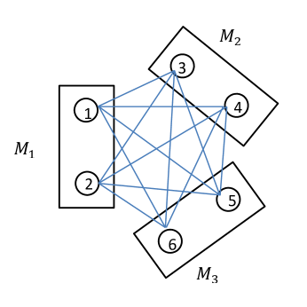
Figure 1: The diamond network: A complete partite graph with $K=3$ components, each containing 2 nodes.

In order to show that sluggish mixing behavior itself need not imply instability, we first examine a complete $K$-partite graph as considered in [12], where the nodes can be partitioned into $K\geq 2$ components. All nodes are connected except those belonging to the same component. Figure 1 depicts an example of a complete partite graph with $K=3$ components, each containing 2 nodes. We will refer to this network as the diamond network, since the edges correspond to those of an eight-faced diamond structure, with the node pairs constituting the three components positioned at the opposite ends of three orthogonal axes.

Denote by $M_{k}\subseteq\{1,\dots,N\}$ the subset of nodes belonging the $k$-th component. Once one of the nodes in component $M_{k}$ is active, other nodes within $M_{k}$ can become active as well, but none of the nodes in the other components $M_{l}$, $l\neq k$, can be active. The necessary stability condition then takes the form $\rho=\sum_{k=1}^{K}\hat{\rho_{k}}<1$, with $\hat{\rho}_{k}=\max_{i\in M_{k}}\rho_{i}$ denoting the maximum traffic intensity of any of the nodes in the $k$-th component.

Now consider the case that each node operates with an activation function $f(x)$ with $\lim_{x\to\infty}f(x)>0$ and a de-activation function $g(x)={\rm o}(x^{-\gamma})$, with $\gamma>1$, which subsumes the random-capture scheme with $g(x)\equiv 0$ for all $x\geq 1$ in [12]. Since the de-activation rate decays so sharply, the probability of a node releasing the medium once it has started transmitting with an initial queue length of order $R$, is vanishingly small, until the queue length falls below order $R$ or the total number of transmissions exceeds order $R$ (but the latter implies the former). Hence, in the fluid limit, a node must completely empty almost surely before it releases the medium. Because of the interference constraints, it further follows that once the activity process enters one of the components, it remains there until all the queues in that component have entirely drained (on the fluid scale), and then randomly switches to one of the other components. For conciseness, the fluid limit process is said to be in an $M_{k}$-period during time intervals when at least one of the nodes in component $M_{k}$ is served at full rate (on the fluid scale).

Based on the above informal observations, we now proceed with a more detailed description of the dynamics of the fluid limit process. We do not aim to provide a proof of the stated properties, since the main goal of the present paper is to demonstrate the potential for instability rather than establish stability. However, the proof arguments that we will develop for a similar but more complicated interference graph in the remainder of the paper, could easily be applied to provide a rigorous justification of the fluid limit and establish the claimed stability results.

Assume that the system enters an $M_{k}$-period at time $t$, then

1. It spends a time period $T_{k}(t)=\max_{i\in M_{k}}\frac{Q_{i}(t)}{\mu_{i}-\lambda_{i}}$ in $M_{k}$.

2. During this period, the queues of the nodes in $M_{k}$ drain at a linear rate (or remain zero)

   $$Q_{i}(t+u)=\max\{Q_{i}(t)+(\lambda_{i}-\mu_{i})u,0\},~{}\forall i\in M_{k},$$

   while the queues of the other nodes fill at a linear rate

   $$Q_{i}(t+u)=Q_{i}(t)+\lambda_{i}u,~{}\forall i\not\in M_{k},$$

   for all $u\in[0,T_{k}(t)]$.

3. At time $t+T_{k}(t)$, the system switches to an $M_{l}$-period, $l\neq k$, with probability

   $$p_{kl}(t+T_{k}(t))=\lim_{R\to\infty}\frac{\sum_{i\in M_{l}}f(RQ_{i}(t+T_{k}(t)))}{\sum_{l^{\prime}\neq k,l}\sum_{i\in M_{l^{\prime}}}f(RQ_{i}(t+T_{k}(t)))}.$$

Thus the fluid limit follows a piece-wise linear sample path, with switches between different periods governed by the transition probabilities specified above. Figure 2 depicts an example of the fluid limit sample path for the network of Figure 1 with $f(x)=1$, $x\geq 1$.

Now define the Lyapunov function $L(t):=\sum_{k=1}^{K}\hat{Q}_{k}(t)$, with $\hat{Q}_{k}(t)=\max_{i\in M_{k}}Q_{i}(t)/\mu_{i}$. Then, $\frac{{\rm d}}{{\rm d}t}L(t)\leq\sum_{k=1}^{K}\hat{\rho}_{k}-1=\rho-1<0$ almost everywhere when $\rho<1$, as long as $L(t)>0$. Therefore, $L(t)=0$, and hence $Q(t)=0$, for all $t\geq T$, with $T=\frac{L(0)}{1-\rho}<\infty$, implying stability [5, 7], even though the fluid limit behavior is not smooth at all.

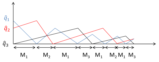
Figure 2: A fluid limit sample path for the diamond network of Figure 1.

IV Fluid limits for broken-diamond network

In the previous section we discussed qualitative features of fluid limits in various scenarios, and in particular for so-called complete partite graphs. We now proceed to consider a ‘nearly’ complete partite graph, and will demonstrate that if some of the edges between two components $M_{k}$ and $M_{l}$ are removed (thus reducing interference), the network might become unstable for ‘aggressive’ activation and/or deactivation functions! Specifically, we will consider the diamond network of Figure 1, and remove the edge between nodes 4 and 5 to obtain a broken-diamond network with an additional component/maximal schedule $M_{4}$, as depicted in Figure 3.

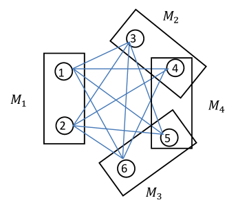
Figure 3: The broken-diamond network, obtained by removing 1 edge from the diamond network of Figure 1, yielding an additional schedule $M_{4}$.

The intuitive explanation for the potential instability may be described as follows. Denote $\rho_{0}=\max\{\rho_{1},\rho_{2}\}$, and assume $\rho_{3}\geq\rho_{4}$ and $\rho_{6}\geq\rho_{5}$. It is easily seen that the fraction of time that at least one of the nodes 1, 2, 3 and 6 is served, must be no less than $\rho=\rho_{0}+\rho_{3}+\rho_{6}$ in order for these nodes to be stable. During some of these periods nodes 4 or 5 may also be served, but not simultaneously, i.e., schedule $M_{4}$ cannot be used. In other words, the system cannot be stable if schedule $M_{4}$ is used for a fraction of the time larger than $1-\rho$. As it turns out, however, when the de-activation function is sufficiently aggressive, e.g., $g(x)={\rm o}(x^{-\gamma})$, with $\gamma>1$, schedule $M_{4}$ is in fact persistently used for a fraction of the time that does not tend to 0 as $\rho$ approaches 1, which forces the system to be unstable.

Although the above arguments indicate that invoking schedule $M_{4}$ is a recipe for trouble, the reason may not be directly evident from the system dynamics, since no obvious inefficiency occurs as long as the queues of nodes 4 and 5 are non-empty. However, the fact that the Lyapunov function $L(t)=\sum_{k=1}^{3}\max_{i\in M_{k}}Q_{i}(t)$ may increase while serving nodes 4 and 5, when $Q_{3}(t)\geq Q_{4}(t)$ and $Q_{6}(t)\geq Q_{5}(t)$, is already highly suggestive. (Such an increase is depicted in Figure 4 during the $M_{4}$ period of the switching sequence $M_{1}\rightarrow M_{2}\rightarrow M_{1}\rightarrow M_{4}\rightarrow M_{3}\rightarrow M_{1}$.) Indeed, serving nodes 4 and 5 may make their queues smaller than those of nodes 3 and 6, leaving these queues to be served by themselves at a later stage, at which point inefficiency inevitably occurs.

In the sequel, the fluid limit process is said to be in a natural state when $Q_{3}(t)\geq Q_{4}(t)$ and $Q_{6}(t)\geq Q_{5}(t)$, with equality only when both sides are zero. We will assume $\lambda_{3}>\lambda_{4}$ and $\lambda_{6}>\lambda_{5}$, and will show that the process must always reside in a natural state after some finite amount of time. As described above, instability is bound to occur when schedule $M_{4}$ is used repeatedly for substantial periods of time while the fluid limit process is in a natural state. Since the process is always in a natural state after some finite amount of time, it is intuitively plausible that such events occur repeatedly with positive probability, but a rigorous proof that this leads to instability is far from simple. Such a proof requires detailed analysis of the underlying stochastic process (in our case via fluid limits), and its conclusion crucially depends on the de-activation function. Indeed, the stability results in [15, 18, 29, 34, 35] indirectly indicate that the broken-diamond network is not rendered unstable for sufficiently cautious de-activation functions.

Just like for the complete partite graphs, the fluid limit process is said to be in an $M_{1}$-period when node 1 or node 2 (or both) is served at full rate. The process is in an $M_{2}$- or $M_{3}$-period when node 3 or 6 is served at full rate, respectively. The process is in an $M_{4}$-period when nodes 4 and 5 are both served at full rate simultaneously.

In Subsection IV-A we will provide a detailed description of the dynamics of the fluid limit process once it has reached a natural state and entered an $M_{1}$-, $M_{2}$-, $M_{3}$ or $M_{4}$-period. The justification for the description follows from a collection of lemmas and propositions which are stated and proved in Appendices A–D, with a high-level outline provided in Subsection IV-B. In Section V we will exploit the properties of the fluid limit process in order to prove that the harmful behavior described above indeed occurs for sufficiently aggressive de-activation functions, implying instability of the fluid limit process as well as the original stochastic process.

IV-A Description of the fluid limit process

We now provide a detailed description of the dynamics of the fluid limit process once it has reached a natural state and entered an $M_{1}$-, $M_{2}$-, $M_{3}$ or $M_{4}$-period. For sufficiently high load, i.e., $\rho$ sufficiently close to 1, a natural state and such a period occur in uniformly bounded time almost surely for any initial state. As will be seen, for de-activation functions $g_{i}(x)={\rm o}(x^{-\gamma})$, with $\gamma>1$, the fluid limit process then follows similar piece-wise linear trajectories, with random switches, as described in the previous section for complete partite graphs and further illustrated in Figure 4. For notational convenience, we henceforth assume $\mu_{i}\equiv 1$, so that $\rho_{i}\equiv\lambda_{i}$, for all $i=1,\dots,N$, and additionally assume activation functions $f_{i}(x)\equiv 1$, $x\geq 1$, for all $i=1,\dots,N$.

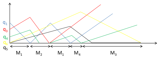
Figure 4: A fluid limit sample path for the broken-diamond network of Figure 3, corresponding to the switching sequence $M_{1}\to M_{2}\to M_{1}\to M_{4}\to M_{3}$.

IV-A1 $M_{1}$-period

Assume the system enters an $M_{1}$-period at time $t$, then

1. It spends a time period $T_{1}(t)=\max\left\{\frac{Q_{1}(t)}{1-\rho_{1}},\frac{Q_{2}(t)}{1-\rho_{2}}\right\}$ in $M_{1}$.

2. During this period, the queues of nodes 1 and 2 drain at a linear rate (or remain zero)

   $$Q_{i}(t+u)=\max\{Q_{i}(t)-(1-\rho_{i})u,0\},\mbox{ for }i=1,2,$$

   while the queues of nodes 3, 4, 5, 6 fill at a linear rate

   $$Q_{i}(t+u)=Q_{i}(t)+\rho_{i}u,\mbox{ for }i=3,4,5,6,$$

   for all $u\in[0,T_{1}(t)]$. In particular, $Q_{1}(t+T_{1}(t))=Q_{2}(t+T_{1}(t))=0$.

3. At time $t+T_{1}(t)$, the system switches to an $M_{2}$-, $M_{3}$- or $M_{4}$-period with transition probabilities $p_{12}=\frac{3}{8}$, $p_{13}=\frac{3}{8}$, and $p_{14}=\frac{1}{4}$, respectively.

IV-A2 $M_{2}$-period

Assume that the system enters an $M_{2}$-period at time $t$, then

1. The system spends a time period $T_{2}(t)=\frac{Q_{3}(t)}{1-\rho_{3}}$ in $M_{2}$.

2. During this period, the queues of nodes 3 and 4 drain (or remain zero)

   $$Q_{i}(t+u)=\max\{Q_{i}(t)-(1-\rho_{i})u,0\},\mbox{ for }i=3,4,$$

   while the queues of nodes 1, 2, 5, 6 fill at a linear rate

   $$Q_{i}(t+u)=Q_{i}(t)+\rho_{i}u,\mbox{ for }i=1,2,5,6,$$

   for all $u\in[0,T_{2}(t)]$. In particular, $Q_{3}(t+T_{2}(t))=0$.

3. At time $t+T_{2}(t)$, the system switches to an $M_{1}$- or $M_{3}$-period. Note that $\frac{Q_{3}(t)}{1-\rho_{3}}>\frac{Q_{4}(t)}{1-\rho_{4}}$ by the assumption that $\lambda_{3}>\lambda_{4}$ and that the process has reached a natural state, so that $Q_{3}(t)>Q_{4}(t)$ (since $Q_{3}(t)=Q_{4}(t)=0$ cannot occur at the start of an $M_{2}$-period). Thus node 4 has emptied before time $t+T_{2}(t)$, and remained empty (on the fluid scale) since then, precluding a switch to an $M_{4}$-period except for a negligible duration on the fluid scale), only allowing the system to switch to either an $M_{1}$- or $M_{3}$-period. The corresponding transition probabilities can be formally expressed in terms of certain stationary distributions, but are difficult to obtain in explicit form. Note that in order for any of the nodes 1, 2, 5 or 6 to activate, node 3 must be inactive. In order for nodes 1, 2 or 6 to activate, node 4 must be inactive as well, but the latter is not necessary in order for node 5 to activate. Since node 4 may be active even when it is empty on the fluid scale, it follows that node 5 enjoys an advantage in competing for access to the medium over nodes 1, 2 and 6. While it may be argued that node 4 is active with probability $\rho_{4}$ by the time node 3 becomes inactive for the first time, the resulting probabilities for the various nodes to gain access to the medium first do not seem to allow a simple expression.

   Remark 1

   If the process had not yet reached a natural state, the case $\frac{Q_{3}(t)}{1-\rho_{3}}\leq\frac{Q_{4}(t)}{1-\rho_{4}}$ could also arise. In case that inequality is strict, i.e., $\frac{Q_{3}(t)}{1-\rho_{3}}<\frac{Q_{4}(t)}{1-\rho_{4}}$, the queue of node 4 is still non-empty by time $t+T_{2}(t)$, simply forcing a switch to an $M_{4}$-period with probability 1.

   In case of equality, i.e., $\frac{Q_{3}(t)}{1-\rho_{3}}=\frac{Q_{4}(t)}{1-\rho_{4}}$, however, the situation would be much more complicated, which serves as the illustration for the significance of the notion of a natural state. In order to describe these difficulties, note that the queues of nodes 3 and 4 both empty at time $t+T_{2}(t)$, barring a switch to an $M_{4}$-period, and permitting only a switch to either an $M_{1}$- or $M_{3}$-period. Just like before, node 5 is the only one able to activate during periods where node 3 is inactive while node 4 is active, and hence enjoys an advantage in competing for access to the medium. In fact, node 5 will gain access to the medium first almost surely if node 3 is the first one to become inactive (in the pre-limit). The probability of that event, and hence the transition probabilities to an $M_{1}$- or $M_{3}$-period, depends on queue length differences between nodes 3 and 4 at time $t$ that can be affected by the history of the process and are not visible on the fluid scale.

IV-A3 $M_{3}$-period

The dynamics for an $M_{3}$-period are entirely symmetric to those for an $M_{2}$-period, but will be replicated below for completeness.

Assume that the system enters an $M_{3}$-period at time $t$, then

1. The system spends a time period $T_{3}(t)=\frac{Q_{6}(t)}{1-\rho_{6}}$ in $M_{3}$.

2. During this period, the queues of nodes 5 and 6 drain (or remain zero)

   $$Q_{i}(t+u)=\max\{Q_{i}(t)-(1-\rho_{i})u,0\},\mbox{ for }i=5,6,$$

   while the queues of nodes 1, 2, 3, 4 fill at a linear rate

   $$Q_{i}(t+u)=Q_{i}(t)+\rho_{i}u,\mbox{ for }i=1,2,3,4,$$

   for all $u\in[0,T_{3}(t)]$. In particular, $Q_{6}(t+T_{3}(t))=0$.

3. At time $t+T_{3}(t)$, the system switches to an $M_{1}$- or $M_{2}$-period. Note that $\frac{Q_{5}(t)}{1-\rho_{5}}<\frac{Q_{6}(t)}{1-\rho_{6}}$ by the assumption that $\lambda_{5}>\lambda_{6}$ and that the process has reached a natural state, so that $Q_{5}(t)<Q_{6}(t)$ (since $Q_{5}(t)=Q_{6}(t)=0$ cannot occur at the start of an $M_{3}$-period).

   Thus node 5 has emptied before time $t+T_{3}(t)$, and remained empty (on the fluid scale) since then, precluding a switch to an $M_{4}$-period (except for a negligible period on the fluid scale), only allowing the system to switch to either an $M_{1}$- or $M_{2}$-period. The corresponding transition probabilities are difficult to obtain in explicit form for similar reasons as mentioned in case 2(c).

   Remark 2

   If the process had not yet reached a natural state, the case $\frac{Q_{5}(t)}{1-\rho_{5}}\geq\frac{Q_{6}(t)}{1-\rho_{6}}$ could also arise. In case that inequality is strict, i.e., $\frac{Q_{5}(t)}{1-\rho_{5}}<\frac{Q_{6}(t)}{1-\rho_{6}}$, the queue of node 5 is still non-empty by time $t+T_{3}(t)$, forcing a switch to an $M_{4}$-period with probability 1.

   In case of equality, i.e., $\frac{Q_{5}(t)}{1-\rho_{5}}=\frac{Q_{6}(t)}{1-\rho_{6}}$, the queues of nodes 5 and 6 both empty at time $T_{3}(t)$, barring a switch to an $M_{4}$-period, and permitting only a switch to either an $M_{1}$- or $M_{2}$-period. For similar reasons as mentioned in case 2(c), the corresponding transition probabilities depend on queue length differences that are affected by the history of the process and are not visible on the fluid scale.

IV-A4 $M_{4}$-period

Assume that the system enters an $M_{4}$-period at time $t$, then

1. It spends a time period $T_{4}(t)=\min\left\{\frac{Q_{4}(t)}{1-\rho_{4}},\frac{Q_{5}(t)}{1-\rho_{5}}\right\}$ in $M_{4}$.

2. During this period, the queues of nodes 4 and 5 drain at a linear rate

   $$Q_{i}(t+u)=Q_{i}(t)-(1-\rho_{i})u,\mbox{ for }i=4,5,$$

   while the queues of nodes 1, 2, 3, 6 fill at a linear rate

   $$Q_{i}(t+u)=Q_{i}(t)+\rho_{i}u,\mbox{ for }i=1,2,3,6,$$

   $u\in[0,T_{4}(t)]$. In particular, $\min\{Q_{4}(t+T_{4}(t)),Q_{5}(t+T_{4}(t))\}=0$.

3. At time $t+T_{4}(t)$, the system switches to either an $M_{2}$- or $M_{3}$-period. In order to determine which of these events can occur, we need to distinguish between three cases, depending on whether $\frac{Q_{4}(t)}{1-\rho_{4}}$ is (i) larger than, (ii) equal to, or (iii) smaller than $\frac{Q_{5}(t)}{1-\rho_{5}}$.

   In case (i), i.e., $\frac{Q_{4}(t)}{1-\rho_{4}}>\frac{Q_{5}(t)}{1-\rho_{5}}$, we have $Q_{4}(t+T_{4}(t))>0$, i.e., the queue of node 4 is still non-empty by time $t+T_{4}(t)$, causing a switch to an $M_{2}$-period with probability 1.

   In case (ii), i.e., $\frac{Q_{4}(t)}{1-\rho_{4}}=\frac{Q_{5}(t)}{1-\rho_{5}}$, we have $Q_{4}(t+T_{4}(t))=Q_{5}(t+T_{4}(t))=0$, i.e., the queues of nodes 4 and 5 both empty at time $t+T_{4}(t)$. Even though both queues empty at the same time on the fluid scale, there will with overwhelming probability be a long period in the pre-limit where one of the nodes has become inactive for the first time while the other one has yet to do so. Since both nodes 4 and 5 must be inactive in order for nodes 1 and 2 to activate, these nodes have no chance to activate during that period, but either node 3 or node 6 does, depending on whether node 5 or node 4 is the first one to become inactive. As a result, the system cannot switch to an $M_{1}$-period, but only to an $M_{2}$- or $M_{3}$-period. In fact, a switch to $M_{2}$ will occur almost surely if node 5 is the first one to become inactive, while a switch to $M_{3}$ will occur almost surely if node 4 is the first one to become inactive. The probabilities of these two scenarios, and hence the transition probabilities to $M_{2}$ and $M_{3}$, depend on queue length differences between nodes 4 and 5 at time $t$ that are affected by the history of the process and are not visible on the fluid scale.

   In case (iii), i.e., $\frac{Q_{4}(t)}{1-\rho_{4}}<\frac{Q_{5}(t)}{1-\rho_{5}}$, we have $Q_{5}(t+T_{4}(t))>0$, i.e., the queue of node 5 is still non-empty by time $t+T_{4}(t)$, forcing a switch to an $M_{3}$-period with probability 1.

Remark 3

As noted in the above description of the fluid limit process, in cases 2(c), 3(c), and 4(c)(ii) the transition probabilities from an $M_{2}$-period to an $M_{1}$- or $M_{3}$-period, from an $M_{3}$-period to an $M_{1}$- or $M_{2}$-period, and from an $M_{4}$- to an $M_{2}$- or $M_{3}$-period, depend on queue length differences that are affected by the history of the process and are not visible on the fluid scale. Depending on whether or not the initial state and parameter values allow for these cases to arise, it may thus be impossible to provide a probabilistic description the evolution of the resulting fluid limit process, even it terms of its entire own history.

IV-B Overview of fluid limit proofs

In the previous subsection we provided a description of the dynamics of the fluid limit process once it has reached a natural state and entered an $M_{1}$, $M_{2}$-, $M_{3}$ or $M_{4}$-period. As was further stated, for $\rho$ sufficiently close to 1, a natural state and such a period occur in uniformly bounded time almost surely for any initial state. The justification for all these properties follows from a series of lemmas and propositions stated and proved in Appendices A–D. In this subsection we present a high-level outline of the fluid limit statements and proofs.

First of all, recall that the description of the fluid limit process referred to the continuous-time Markov process representing the system dynamics as introduced in Section II. For all the proofs of fluid limit properties and instability results however we consider a rescaled linear interpolation of the uniformized jump chain (as defined in Appendix A.I). This construction yields convenient properties of the fluid limit paths and allows us to extend the framework of Meyn [27] for establishing instability results for discrete-time Markov chains. (The original continuous-time Markov process has in fact the same fluid limit properties, but this is not directly relevant in any of the proofs.)

The proofs of the fluid limit properties consist of four main parts. Part A identifies several basic properties of the fluid limit paths, and in particular establishes that the queue length trajectory of each of the individual nodes exhibits ‘sawtooth’ behavior. This fundamental property in fact holds in arbitrary interference graphs, and only requires an exponent $\gamma>1$ in the backoff probability. Part B of the proof shows a certain dominance property, saying that if all the interferers of a particular node also interfere with some other node that is currently being served at full rate, then the former node must be empty or served at full rate (on the fluid scale) as well. Under the assumption $\lambda_{3}>\lambda_{4}$, $\lambda_{5}<\lambda_{6}$, the dominance property implies that after a finite amount of time the fluid limit process for the broken-diamond network must always reside in a natural state as defined in the previous subsection. Part C of the proof centers on the $M_{1}$-, $M_{2}$-, $M_{3}$- and $M_{4}$-periods, and establishes that at the end of any such period, the process immediately switches to one of the other types of periods with the probabilities indicated in the previous subsection. In particular, it is deduced that an $M_{4}$-period cannot be entered from an $M_{2}$- or $M_{3}$-period, and must always be preceded by an $M_{1}$-period once the process has reached a natural state. The combination of the sawtooth queue length trajectories and the switching probabilities provides a probabilistic description of the dynamics of the fluid limit once the process has reached a natural state and entered an $M_{1}$-, $M_{2}$-, $M_{3}$- or $M_{4}$-period. Part B already established that the process must always reside in a natural state after a finite amount of time, but it remains to be shown that the process will inevitably enter an $M_{1}$-, $M_{2}$-, $M_{3}$- or $M_{4}$- period, which constitutes the final Part D of the proof. The core argument is that interfering empty and nonempty queues can not coexist, since the empty nodes will frequently enter back-off periods, offering the nonempty nodes abundant opportunities to gain access, drain their queues, and cause the empty nodes to build queues in turn.

Part A of the proof starts with the simple observation that, by the “ skip-free” property of the original pre-limit process, the sample paths of the interpolated version of the uniformized jump chain are Lipschitz continuous, and hence so are the sample paths of the fluid-scaled process. The fluid limit paths inherit the Lipschitz continuity, and are thus differentiable almost everywhere with probability one.

Then fluid limit paths are determined by a countable set of ‘entrance’ times and ‘exit’ times of $(0,\infty)$ with probability one. The proof then proceeds to show that if a nonempty node (on the fluid scale) receives any amount of service during some time interval, then it must in fact be served at the full rate until it has completely emptied (on the fluid scale), assuming $\gamma>1$. This implies that when node $i$ is nonempty (on the fluid scale), its queue must either increase at rate $\lambda_{i}$ or decrease at rate $1-\lambda_{i}$ until it has entirely drained. In other words, the queue length trajectory of each of the individual nodes exhibits sawtooth behavior (Theorem 5).

Part B of the proof pertains to the joint behavior of the fluid limit trajectories of the various queue lengths. First of all, the natural property is proved that whenever a particular node is served, none of its interferers can receive any service (Lemma 3). Second, it is established that whenever a particular node is served, any node whose interferers are a subset of those of the node served, must either be empty or be served at full rate as well (on the fluid scale) (Corollary 3). For example, in the broken-diamond network, whenever node 3 is served, node 4 must either be empty or be served at full rate as well, and similarly for nodes 5 and 6. These two properties combined yield a dominance property, saying that if all the interferers of a particular node also interfere with some other node that is currently being served at full rate, then the former node must be empty or served at full rate (on the fluid scale) as well. In the case of the broken-diamond network, under the assumption $\lambda_{3}>\lambda_{4}$, the queue of node 3 will therefore never be smaller than that of node 4 after some finite amount of time, and similarly for nodes 4 and 5. Thus the fluid limit process will always reside in a natural state after some finite amount of time.

Part C of the proof focuses on the $M_{1}$-, $M_{2}$-, $M_{3}$- and $M_{4}$-periods as described above. Because of the sawtooth behavior, an $M_{1}$-period can only end when both nodes 1 and 2 are empty (on the fluid scale). Likewise, an $M_{2}$- or $M_{3}$-period can only end when node 3 or node 6 is empty, respectively. An $M_{4}$-period can only end when node 4 or node 5 (or both) is empty. It is then proven that at the end of an $M_{1}$-period, the fluid limit process immediately switches to an $M_{2}$-, $M_{3}$- or $M_{4}$-period with the probabilities specified in the previous subsection (Theorem 7). When the process resides in a natural state, an $M_{2}$-period is always instantaneously followed by an $M_{1}$- or $M_{3}$-period, while an $M_{3}$-period is always instantaneously followed by an $M_{1}$- or $M_{2}$-period. In particular, it is concluded that an $M_{4}$-period cannot be entered from an $M_{2}$- or $M_{3}$-period, and must always be preceded by an $M_{1}$-period once the process has reached a natural state. After an $M_{4}$-period, the process always immediately switches to an $M_{2}$- or $M_{3}$-period.

There is no reason a priori however that the process is guaranteed to actually ever enter an $M_{1}$-, $M_{2}$-, $M_{3}$- or $M_{4}$- period. In fact, the process may very well spend time in different kinds of states, but the final Part D of the proof establishes that these kinds of states are transient, and cannot occur once a natural state has been reached, which is forced to happen in a finite amount of time for particular arrival rates as was already shown in Part B. Note that an $M_{1}$-, $M_{2}$-, $M_{3}$- or $M_{4}$- period occurs as soon as node 1, node 2, node 3, node 6 or nodes 4 and 5 simultaneously are served at full rate. In other words, the only ways for the process to avoid an $M_{1}$-, $M_{2}$-, $M_{3}$- or $M_{4}$-period, are: (i) for node 4 to be served at full rate, but not nodes 3 and 5; (ii) for node 5 to be served at full rate, but not nodes 4 and 6; (iii) for none of the nodes to be served at full rate. Scenario (i) requires node 3 to be empty (on the fluid scale) and node 4 to be nonempty, which can not occur in a natural state. Likewise, scenario (ii) cannot arise in a natural state either. Scenario (iii) requires that every empty node $i$ is served at rate $\rho_{i}$ (on the fluid scale), while all nonempty nodes are served at rate 0. Such a scenario is not particularly plausible, but a rigorous proof turns out to be quite involved. The insights rely strongly on the specific properties of the broken-diamond network, and an extension to arbitrary graphs does not seem straightforward. The core argument is that interfering empty and nonempty queues can not coexist, since the empty nodes will frequently enter back-off periods, offering the nonempty nodes abundant opportunities to gain access, drain their queues, and cause the empty nodes to build queues in turn.

V Instability results for broken-diamond network

In the previous section we provided a detailed description of the dynamics of the fluid limit process once it has reached a natural state and entered an $M_{1}$-, $M_{2}$-, $M_{3}$ or $M_{4}$-period. In this section we exploit the properties of the fluid limit process in order to prove that it is unstable for $\rho$ sufficiently close to 1, and then show how the instability of the original stochastic process can be deduced from the instability of the fluid limit process.

V-A Instability of the fluid limit process

In order to prove instability of the fluid limit process, we first revisit the intuitive explanation discussed earlier, see Figure 4 for an illustration. Denote $\rho_{0}=\max\{\rho_{1},\rho_{2}\}$, and recall that $\rho_{3}\geq\rho_{4}$ and $\rho_{5}\leq\rho_{6}$ by assumption. Since nodes 1, 2, 3 and 6 are only served during $M_{1}$-, $M_{2}$- and $M_{3}$-periods, and not during $M_{4}$-periods, it is easily seen that the fraction of time that the system spends in $M_{1}$-, $M_{2}$- and $M_{3}$-periods must be no less than $\rho=\rho_{0}+\rho_{3}+\rho_{6}$ in order for these nodes to be stable. Thus, the system cannot be stable if it spends a fraction of the time larger than $1-\rho$ in $M_{4}$-periods. As it turns out, however, when the de-activation function is sufficiently aggressive, e.g., $g(x)={\rm o}(x^{-\gamma})$, with $\gamma>1$, $M_{4}$-periods in fact persistently occur for a fraction of time that does not tend to 0 as $\rho$ approaches 1, which forces the system to be unstable.

Figure 4 shows a fluid-limit sample path corresponding to the switching sequence $M_{1}\to M_{2}\to M_{1}\to M_{4}\to M_{3}\to M_{1}$. The aggregate queue size starts building up in the $M_{3}$-period that follows the $M_{4}$-period.

In order to prove instability of the fluid limit process, we adopt the Lyapunov function $L(t)=\sum_{k=1}^{3}\max_{i\in M_{k}}Q_{i}(t)$, and will show that the load $L(t)$ grows without bound almost surely. Note that the load $L(t)$ increases during $M_{4}$-periods while the process is in a natural state.

In preparation for the instability proof, we first state two auxiliary lemmas. It will be convenient to view the evolution of the fluid limit process, and in particular the Lyapunov function $L(t)$, over the course of cycles. The $i$-th cycle is the period from the start of the $(i-1)$-th $M_{1}$-period to the start of the $i$-th $M_{1}$-period once the fluid limit process has reached a natural state. Denote by $t_{i}$ the start time of the $i$-th cycle, $i=1,2,\dots$. Each $t_{i}$ is finite almost surely for $\rho$ sufficiently close to 1, and in particular an infinite number of cycles must occur almost surely. In order to see that, recall that the fluid limit process will reach a natural state and enter an $M_{1}$, $M_{2}$, $M_{3}$- or $M_{4}$-period in finite time almost surely for any initial state as stated in Subsection IV-A. The description of the dynamics of the fluid limit process provided in that subsection then implies that $M_{1}$-periods and hence cycles must occur infinitely often (and if only finitely many $M_{1}$-periods occurred, then at least one of the nodes would in fact never be served again after some finite time, implying that the fluid limit process is unstable regardless).

The next lemma shows that the duration of a cycle and the possible increase in the load over the course of a cycle are linearly bounded in the load at the start of the cycle.

Lemma 1

The duration of the $i$-th cycle, $\Delta t_{i}=t_{i+1}-t_{i}$, and the increase in the load over the course of the $i$-th cycle, $L(t_{i+1})-L(t_{i})=L(t_{i}+\Delta t_{i})-L(t_{i})$, are bounded from above by

$$\Delta t_{i}\leq C_{T}L(t_{i})\mbox{ and }L(t_{i+1})-L(t_{i})\leq C_{L}L(t_{i}),$$

for all $\rho\leq 1$, where $C_{T}=\frac{1}{1-\rho_{3}-\rho_{6}}\left(\frac{1}{1-\rho_{0}}+\frac{1}{1-\max\{\rho_{4},\rho_{5}\}}\right)$ and $C_{L}=\frac{\rho}{1-\max\{\rho_{4},\rho_{5}\}}$.

The proof of the above lemma is presented in Appendix E.

In order to establish that the durations of $M_{4}$-periods are non-negligible, it will be useful to introduce the notion of ‘weakly-balanced’ queues, ensuring that the queues of nodes 4 and 5 are not too small compared to the queues of nodes 3 and 6.

Definition 1

Let $\beta^{\min}$ and $\beta^{\max}$ be fixed positive constants. The queues are said to be weakly-balanced in a given cycle (with respect to $\beta^{\min}$ and $\beta^{\max}$) if $\beta^{\min}\leq\frac{Q_{3}(t)}{Q_{5}(t)},\frac{Q_{6}(t)}{Q_{4}(t)}\leq\beta^{\max}$, with $t$ denoting the time when the $M_{1}$-period ends that initiated the cycle.

The next lemma shows that over two consecutive cycles, the queues will be weakly-balanced with probability at least 1/3.

Lemma 2

Let

$$\epsilon=\frac{\rho_{2}}{2\left(\rho_{2}+(\rho_{3}+\rho_{6})\frac{1-\min\{\rho_{4},\rho_{5}\}}{1-\max\{\rho_{4},\rho_{5}\}}\right)}\geq\frac{\rho_{2}}{\rho}\frac{1-\max\{\rho_{4},\rho_{5}\}}{1-\min\{\rho_{4},\rho_{5}\}}.$$

Then over two consecutive cycles, with probability at least 1/3, the queues will be weakly-balanced in at least one of these cycles with

$$\beta^{\max}=\frac{\max\{\rho_{3},\rho_{6}\}+(1-\rho_{2})(1-\epsilon)/\epsilon}{\min\{\rho_{4},\rho_{5}\}},$$

and $\beta^{\min}=\frac{1}{\beta^{\max}}$.

The proof of the above lemma is presented in Appendix E.

As suggested by the above lemma, it will be convenient to consider pairs of two consecutive cycles in order to prove instability of the fluid limit process.

Let $D_{k}$ be the pair of cycles consisting of cycles $2k-1$ and $2k$ as in Figure 5, $k=1,2,\dots$. With minor abuse of notation, denote by $T_{k}=t_{2k-1}$ the start time of $D_{k}$ and $L_{k}=L(T_{k})$. Denote by $\Delta T_{k}=T_{k+1}-T_{k}$ the duration of $D_{k}$ and by $\Delta L_{k}=L_{k+1}-L_{k}$ the increase in $L(t)$ over the course of $D_{k}$.

The next proposition shows that for $\rho$ sufficiently close to 1 the load cannot significantly decrease over a pair of cycles and will increase by a substantial amount with non-zero-probability. We henceforth assume $(\rho_{1},\rho_{2},\rho_{3},\rho_{4},\rho_{5},\rho_{6})=\rho(\kappa_{1},\kappa_{2},\kappa_{3},\kappa_{3}-\alpha,\kappa_{6}-\alpha,\kappa_{6})$, with $\max\{\kappa_{1},\kappa_{2}\}+\kappa_{3}+\kappa_{6}=1$ and $0<\alpha<\min\{\kappa_{3},\kappa_{6}\}$, so that $\rho=\rho_{0}+\rho_{3}+\rho_{6}$.

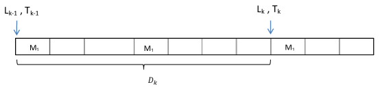
Figure 5: A cycle $D_{k}$ consisting of a pair of consecutive cycles.

Proposition 1

Let $C_{LT}=C_{T}(2+C_{L})$, with $C_{T}$ and $C_{L}$ as specified in Lemma 1, $\theta=1-(1-\rho)C_{LT}$, $p=1/12$. Over cycle pairs $D_{k}$, $k=1,2,\dots$,

• $\Delta T_{k}\leq C_{LT}L_{k}$;

• $L(t)\geq\theta L_{k}$ for all $t\in[T_{k},T_{k+1}]$;

• ${\mathbb{P}}\bigl{(}L_{k+1}-\theta L_{k}\geq\delta(\rho)\theta L_{k}|L_{k}\bigr{)}\geq p$,

with $\delta(\rho)$ a constant, depending on $\rho$, and $\delta(\rho)\uparrow\delta=\frac{1}{\beta^{\max}(1+\beta^{\max})(1+\alpha-\min\{\kappa_{3},\kappa_{6}\})}$, as $\rho\uparrow 1$.

Proof:

We first show part (i). Using Lemma 1, we find

$$\Delta T_{k}=\Delta t_{2k-1}+\Delta t_{2k}\leq C_{T}(L(t_{2k-1})+L(t_{2k}))\leq C_{T}(2+C_{L})L_{k}.$$

In order to prove part (ii), note that $L(t)$ cannot decrease at a larger rate than $1-\rho$, so that in view of part (i),

$$L(t)\geq L_{k}-(1-\rho)(t-T_{k})\geq L_{k}-(1-\rho)\Delta T_{k}\geq(1-(1-\rho)C_{LT})L_{k}=\theta L_{k},$$

for all $t\in[T_{k},T_{k+1}]$.

We now turn to part (iii). Suppose that the following event occurs: the queues are weakly-balanced at the end of an $M_{1}$-period, say time $\tau$, during $D_{k}$ (which according to Lemma 2) happens with at least probability 1/3) and the system then enters an $M_{4}$-period (which happens with probability 1/4). Recalling that $\rho_{3}>\rho_{4}$, $Q_{3}(t)\geq Q_{4}(t)$, $\rho_{5}<\rho_{6}$ and $Q_{5}(t)\leq Q_{6}(t)$, we find that during the $M_{4}$-period $L(t)$ increases by

$$\rho\min\left\{\frac{Q_{4}(\tau)}{1-\rho_{4}},\frac{Q_{5}(\tau)}{1-\rho_{5}}\right\}\geq\rho\frac{\min\{Q_{4}(\tau),Q_{5}(\tau)\}}{1-\rho\min\{\kappa_{3},\kappa_{6}\}+\rho\alpha}.$$

Since the queues are weakly-balanced, we deduce $Q_{3}(\tau)\leq\beta^{\max}Q_{5}(\tau)\leq\beta^{\max}Q_{6}(\tau)\leq(\beta^{\max})^{2}Q_{4}(\tau)$ and $Q_{6}(\tau)\leq\beta^{\max}Q_{4}(\tau)\leq\beta^{\max}Q_{3}(\tau)\leq(\beta^{\max})^{2}Q_{5}(\tau)$. Noting that $Q_{1}(\tau)=Q_{2}(\tau)=0$, we obtain

$$L(\tau)=Q_{3}(\tau)+Q_{6}(\tau)\leq(1+\beta^{\max})Q_{6}(\tau)\leq\beta^{\max}(1+\beta^{\max})Q_{4}(\tau),$$

and also

$$L(\tau)=Q_{3}(\tau)+Q_{6}(\tau)\leq(1+\beta^{\max})Q_{3}(\tau)\leq\beta^{\max}(1+\beta^{\max})Q_{5}(\tau).$$

So

$$L(\tau)\leq\beta^{\max}(1+\beta^{\max})\min\{Q_{4}(\tau),Q_{5}(\tau)\},$$

and thus the increase in $L(t)$ during the $M_{4}$-period is no less than $\delta(\rho)L(\tau)$, with

$$\delta(\rho)=\frac{\rho}{\beta^{\max}(1+\beta^{\max})(1-\rho\min\{\kappa_{3},\kappa_{6}\}+\rho\alpha)}.$$

Using part (i) once again, we conclude that with at least probability 1/12,

$$L_{k+1} \geq L_{k}+\delta(\rho)L(\tau)-(1-\rho)\Delta T_{k}\geq L_{k}+\delta(\rho)(L_{k}-(1-\rho)\Delta T_{k})-(1-\rho)\Delta T_{k}$$

$$= (1+\delta(\rho))(L_{k}-(1-\rho)\Delta T_{k})\geq(1+\delta(\rho))(L_{k}-(1-\rho)C_{LT}L_{k})$$

$$= (1+\delta(\rho))\theta L_{k}.$$

∎

Armed with the above proposition, we now proceed to prove that the fluid limit process is unstable, in the sense that $L(T)\to\infty$ as $T\to\infty$. In fact, $L(T)$ grows faster than any sub-linear function $T^{\frac{1}{m}}$, $m>1$, as stated in the next theorem.

Theorem 1

For any $m>1$, there exists a constant $\rho^{*}=\rho^{*}(\kappa,m)<1$, such that for all $\rho\in(\rho^{*},1]$,

$$\limsup_{T\to\infty}{\mathbb{E}}\left[{\displaystyle\frac{T}{L^{m}(T)}}\right]=0,$$

for any initial state ${\bf Q}(0)$ with $\lvert\lvert{\bf Q}(0)\rvert\rvert=1$, and $\lvert\lvert\cdot\rvert\rvert$ denoting the $L_{1}$-norm.

Proof:

Consider the cycle pairs $D_{k}$, $k=1,2,\dots$, as defined right before Proposition 1. Assume $\rho\in(1-\frac{1}{C_{LT}},1]$, so that $\theta\in(0,1]$ in Proposition 1. For any time $t>T_{1}$, we can define a stopping time $N_{t}$ such that $T_{N_{t}}<t\leq T_{N_{t}+1}$, i.e., $t$ is within the $N_{t}$-th cycle pair. (This is possible almost surely, since $T_{k}\to\infty$ as $k\to\infty$ almost surely, as will be proven below.) Recall that $T_{N_{t}+1}\leq T_{N_{t}}+C_{LT}L_{N_{t}}$ and $L(t)\geq\theta L_{N_{t}}$ by parts (i) and (ii) of Proposition 1, respectively, and trivially $L_{N_{t}}\leq L(0)+\rho T_{N_{t}}\leq 2T_{N_{t}}$ for $t$ sufficiently large. Thus,

$$\limsup_{t\to\infty}{\mathbb{E}}\left[{\displaystyle tL^{-m}(t)}\right] \leq \limsup_{t\to\infty}{\mathbb{E}}\left[{\displaystyle T_{N_{t}+1}\theta^{-m}L^{-m}_{N_{t}}}\right]$$ (1)

$$\leq \theta^{-m}\limsup_{t\to\infty}{\mathbb{E}}\left[{\displaystyle T_{N_{t}}L^{-m}_{N_{t}}}\right]+\theta^{-m}C_{LT}\limsup_{t\to\infty}{\mathbb{E}}\left[{\displaystyle L^{-m+1}_{N_{t}}}\right]$$

$$\leq \theta(1+2C_{LT})\limsup_{t\to\infty}{\mathbb{E}}\left[{\displaystyle T_{N_{t}}L^{-m}_{N_{t}}}\right].$$

So it suffices to prove that there exists $\rho^{*}=\rho^{*}(\kappa,m)<1$ such that (1) is zero for $\rho>\rho^{*}$, which we now proceed to show.

First of all, by Proposition 1, for any $m>0$,

$${\mathbb{E}}\left[{\displaystyle L_{k+1}^{-m}|{\mathcal{F}}_{k}}\right] \leq (1-p)(\theta L_{k})^{-m}+p((\theta+\delta)L_{k})^{-m}$$ (2)

$$= \alpha_{m}L_{k}^{-m},$$

where ${\mathcal{F}}_{k}$ is a suitable filtration and $\alpha_{m}:=(1-p)\theta^{-m}+p(\theta+\delta)^{-m}$.

Since $\theta(\rho)\to\theta(1)=1$ and $\delta(\rho)\to\delta(1)=\delta>0$ as $\rho\uparrow 1$, $\alpha_{m}(\rho)$ is a continuous function of $\rho$ in the vicinity of 1. Because $\alpha_{m}(1)<1$, there must exist a $\rho_{m}^{*}=\rho^{*}(\kappa,m)<1$ such that $\alpha_{m}<1$ for all $\rho>\rho^{*}$. This shows that, for $\rho>\rho_{m}^{*}$, $L^{-m}_{k}$ is a positive (geometric) supermartingale with parameter $\alpha_{m}<1$. Taking expectations on both sides of (2) yields

$${\mathbb{E}}\left[{\displaystyle L^{-m}_{k}}\right]\leq\alpha_{m}^{k}L^{-m}_{0}.$$ (3)

with $L_{0}=L(t_{i_{0}})>0$ as noted earlier. In particular, $\lim_{k\to\infty}{\mathbb{E}}\left[{\displaystyle L^{-m}_{k}}\right]=0$, and $1/L_{k}\to 0$ almost surely as $k\to\infty$ by the Doob’s supermartingale-convergence Theorem (page 147 of [31]). This implies that $T_{k}\to\infty$ almost surely because $L_{k}\leq\rho T_{k}+1\leq T_{k}+1$. Therefore, the stopping time $T_{N_{t}}$ is well-defined.

Next, consider the sequence of random variables $T_{k}L_{k}^{-m}$. Using Proposition 1,

$${\mathbb{E}}\left[{\displaystyle T_{k}L_{k}^{-m}|{\mathcal{F}}_{k-1}}\right] \leq (T_{k-1}+C_{LT}L_{k-1}){\mathbb{E}}\left[{\displaystyle L_{k}^{-m}|{\mathcal{F}}_{k-1}}\right]$$ (4)

$$\leq (T_{k-1}+C_{LT}L_{k-1})\alpha_{m}L_{k-1}^{-m}$$

$$= \alpha_{m}T_{k-1}L_{k-1}^{-m}+\alpha_{m}C_{LT}L_{k-1}^{-m+1}.$$

Define $\epsilon_{k}:=C_{LT}\alpha_{m}L_{k}^{-m+1}$, then, by (2) and (3), $\epsilon_{k}$ is a positive (geometric) super-martingale with parameter $\alpha_{m-1}<1$ for $\rho>\rho_{m-1}^{*}=\rho^{*}(\kappa,m-1)$. Then, $\sum_{k=1}^{\infty}{\mathbb{E}}\left[{\displaystyle\epsilon_{k}}\right]\leq C_{LT}\alpha_{m}\sum_{k=1}^{\infty}\alpha_{m-1}^{k}<\infty$, which shows that $\lim_{k\to\infty}T_{k}L_{k}^{-m}=0$ almost surely. In particular, define $\alpha:=\max(\alpha_{m},\alpha_{m-1})$ and $\rho^{*}=\max\{\rho_{m}^{*},\rho_{m-1}^{*}\}$, then taking expectations on both sides of (4) yields

$${\mathbb{E}}\left[{\displaystyle T_{k}L_{k}^{-m}}\right]\leq\alpha{\mathbb{E}}\left[{\displaystyle T_{k-1}L_{k-1}^{-m}}\right]+\alpha C_{LT}\alpha^{k-1},$$ (5)

which, by induction, shows that

$${\mathbb{E}}\left[{\displaystyle T_{k}L_{k}^{-m}}\right]\leq\alpha^{k-1}({\mathbb{E}}\left[{\displaystyle T_{1}L_{1}^{-m}}\right]+C_{LT}(k-1)\alpha),$$ (6)

for $\rho\in(\rho^{*},1]$. Now observe that $T_{1}$ is strictly bounded and $L_{1}$ is bounded away from zero, since a natural state is reached in finite time, before the system can empty, almost surely. It then follows that $\lim_{k\to\infty}{\mathbb{E}}\left[{\displaystyle T_{k}L^{-m}_{k}}\right]=0$,

The fact that $T_{k}L_{k}^{-m}$ converges in $\mathcal{L}_{1}$ implies that the sequence of random variables $T_{k}L_{k}^{-m}$ is Uniformly Integrable (UI) (page 147, Theorem 50.1 of [31]). It therefore follows, by adapting the arguments of Doob’s optional sampling theorem (page 159 of [31]), that the family of random variables $\{T_{N_{t}}L^{-m}_{T_{N_{t}}}\}$ is also UI. Thus by definition, given $\varepsilon>0$, there exists $K_{\varepsilon}$ such that

$${\mathbb{E}}\left[{\displaystyle T_{N_{t}}L^{-m}_{N_{t}}{\rm I}_{\left\{{\displaystyle T_{N_{t}}L^{-m}_{N_{t}}\geq K_{\varepsilon}}\right\}}}\right]\leq\varepsilon,~{}~{}\forall t>0$$

We deduce

$${\mathbb{E}}\left[{\displaystyle T_{N_{t}}L^{-m}_{N_{t}}}\right] \leq\sum_{k=1}^{\infty}{\mathbb{E}}\left[{\displaystyle T_{k}L^{-m}_{k}{\rm I}_{\left\{{\displaystyle N_{t}=k}\right\}}{\rm I}_{\left\{{\displaystyle T_{N_{t}}L^{-m}_{N_{t}}\leq K_{\varepsilon}}\right\}}}\right]+\varepsilon$$

$$\leq K_{\varepsilon}{\mathbb{P}}\left\{{\displaystyle N_{t}\leq D}\right\}+\sum_{k=D+1}^{\infty}C_{LT}k\alpha^{k-1}+\varepsilon.$$

Fixing $\varepsilon$ and $D$, we find that

$$\limsup_{t\to\infty}{\mathbb{E}}\left[{\displaystyle T_{N_{t}}L^{-m}_{N_{t}}}\right]\leq(D+1)\frac{\alpha^{D}}{1-\alpha}+\varepsilon$$

by the Monotone Convergence Theorem [1], and thus, letting $D\to\infty$ and $\varepsilon\to 0$, we have $\limsup_{t\to\infty}{\mathbb{E}}\left[{\displaystyle T_{N_{t}}L^{-m}_{N_{t}}}\right]=0$ for $\rho>\rho^{*}$. ∎

Corollary 1

For any $m>1$, there exists a constant $\rho^{*}=\rho^{*}(\kappa,m)<1$, such that for all $\rho\in(\rho^{*},1]$,

$$\liminf_{T\to\infty}\frac{L(T)}{T^{1/m}}=\infty,$$

almost surely for any initial state ${\bf Q}(0)$ with $\lvert\lvert{\bf Q}(0)\rvert\rvert=1$.

Proof:

Note that for any initial state ${\bf Q}(0)$ with $\lvert\lvert{\bf Q}(0)\rvert\rvert=1$,

$$\liminf_{T\to\infty}\frac{L(T)}{T^{1/m}}\geq\liminf_{k\to\infty}\frac{\theta L_{k}}{T_{k+1}^{1/m}},$$

as can be seen from Proposition 1, and so it suffices to show that $\limsup_{k}T_{k+1}L_{k}^{-m}=0$. But $T_{k+1}\leq T_{k}+C_{LT}L_{k}$, thus,

$$\limsup_{k\to\infty}T_{k+1}L_{k}^{-m}\leq\limsup_{k\to\infty}T_{k}L_{k}^{-m}+C_{LT}\limsup_{k\to\infty}L_{k}^{-m+1}.$$ (7)

The right-hand side is zero because, as we saw in the proof of Theorem 1, both $T_{k}L_{k}^{-m}$ and $L_{k}^{-m+1}$ converge to zero almost surely for $\rho\in(\rho^{*}(\kappa,m),1]$.

∎

V-B Instability of the original stochastic process

In Theorem 1 we established that the fluid limit process in unstable, in the sense that $L(T)\to\infty$ as $T\to\infty$. We now proceed to show how the instability of the original stochastic process can be deduced from the instability of the fluid limit process. The original stochastic process is said to be unstable when $\{(U(t),X(t))\}_{t\geq 0}$ is transient, and $\|X(t)\|\to\infty$ almost surely for any initial state $X(0)$.

We will exploit similar arguments as developed in Meyn [27]. A notable distinction is that the result in [27] requires that a suitable Lyapunov function exhibits strict growth over time. In our setting the fluid limit is random, and the growth behavior as stated in Theorem 1 is not strict, but only in expectation and in an asymptotic sense, which necessitates a somewhat delicate extension of the arguments in [27].

The next theorem states the main result of the present paper, indicating that aggressive deactivation functions cause the network of Figure 3 to be unstable for load values $\rho$ sufficiently close to 1.

Theorem 2

Consider the network of Figure 3, and suppose that $f_{i}(x)\equiv 1$, $x\geq 1$, and $g_{i}(x)={\rm o}(x^{-\gamma})$, with $\gamma>1$. Let $(\rho_{1},\rho_{2},\rho_{3},\rho_{4},\rho_{5},\rho_{6})=\rho(\kappa_{1},\kappa_{2},\kappa_{3},\kappa_{3}-\alpha,\kappa_{6}-\alpha,\kappa_{6})$, with $\max\{\kappa_{1},\kappa_{2}\}+\kappa_{3}+\kappa_{6}=1$, and $0<\alpha<\min\{\kappa_{3},\kappa_{6}\}$. Then there exists a constant $\rho^{\star}(\kappa,\alpha)<1$, such that for all $\rho\in(\rho^{\star}(\kappa,\alpha),1]$:

$$\lim_{\|X(0)\|\to\infty}\mathbb{P}_{X(0)}\{\liminf_{t\to\infty}\|X(t))\|=\infty\}=1.$$

Since our Markov Chain is irreducible, Theorem immediately implies that it is transient. The proof of Theorem 2 relies on similar arguments as developed in the proof of Theorem 3.2 in [27]. A crucial role is played by Theorem 3.1 of [27], which is reproduced below for completeness.

Theorem 3

Suppose that for a Markov chain $\{X(n);n=0,1,2,\dots\}$ with discrete state space $S$, there exist positive functions $W(\cdot)$ and $\Delta(\cdot)$ on $S$, and a positive constant $c_{0}$, such that

$${\mathbb{E}}\left[{\displaystyle W(X(n+1))|{\mathcal{F}}_{n}}\right]\leq W(X(n))-\Delta(X(n)),$$ (8)

whenever $X(n)\in S_{c_{0}}=\{x\in S:W(x)\leq c_{0}\}$, with ${\mathcal{F}}_{n}:=\sigma(X(0),X(1),\dots,X(n))$. Then for all $x\in S$,

$${\mathbb{P}}_{x}\left\{\sum_{n=0}^{\infty}\Delta(X(n))<\infty\right\}\geq 1-W(x)/c_{0}.$$

In order to apply the above theorem, we need to construct suitable functions $W(\cdot)$ and $\Delta(\cdot)$. The proof details are presented in Appendix E.

Remark 4

Recall that the class of deactivation functions $g_{i}(x)={\rm o}(x^{-\gamma})$ includes the random-capture scheme with $g(x)\equiv 0$, $x\geq 1$, as considered in [12]. The result in Theorem 2 thus disproves the conjecture that the random-capture scheme is throughput-optimal in arbitrary topologies.

VI Simulation experiments

We now discuss the simulation experiments that we have conducted to support and illustrate the analytical results. Consider the broken-diamond network as depicted Figure 3 and considered in the previous sections. In the simulation experiments, the relative traffic intensities are assumed to be $\kappa_{1}=\kappa_{2}=0.4$, $\kappa_{3}=0.4$, and $\kappa_{6}=0.2$ with $\alpha=0$, for the components $M_{1}$, $M_{2}$, and $M_{3}$, respectively, with a normalized load of $\rho=0.97$. At each node $i$, the initial queue size is $X_{i}(0)=500$, the activation function is $f_{i}(x)\equiv 1$, $x\geq 1$, and the de-activation function is $g_{i}(x)=(1+x)^{-\gamma}$, where we set $\gamma=2$.

Figure 6 plots the evolution of the queue sizes at the various nodes over time, and shows that once a node starts transmitting, it will continue to do so until the queue lengths of all nodes in its component have largely been cleared. This characteristic, and the associated oscillations in the queues, strongly mirror the qualitative behavior displayed by the fluid limit.

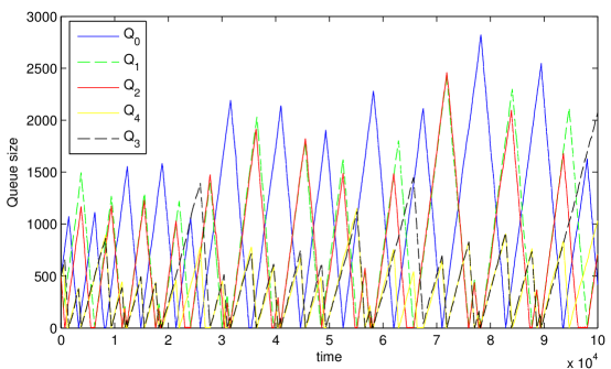
Figure 6: Queue sizes at the various nodes as function of time for the network of Figure 3.

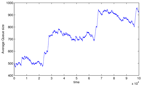
Figure 7: Node-average queue size as function of time for the network of Figure 3.

Although Figure 6 suggests an upward trend in the overall queue lengths, the fluctuations make it hard to discern a clear picture. Figure 7 therefore plots the evolution of the node-average queue size over time, and reveals a distinct growth pattern. Evidently, it is difficult to make any conclusive statements concerning stability/instability based on simulation results alone. However, the saw-tooth type growth pattern in Figure 7 demonstrates strong signs of instability, and corroborates the qualitative growth behavior exhibited by the fluid limit. Indeed, careful inspection of the two figures confirms that the large increments in the node-average queue size occur immediately after $M_{4}$-periods, exactly as predicted by the fluid limit. We further observe that in between these periods, the node-average queue size tends to follow a slightly downward trend, consistent with the negative drift of rate $(\rho-1)/3$ in the fluid limit.

VII Concluding remarks and extensions

We have used fluid limits to demonstrate the potential instability of queue-based random-access algorithms. For the sake of transparency, we focused on a specific six-node network and super-linear activity functions. Similar instability issues can however arise in a far broader class of interference graphs, as we will discuss in Subsection VII-A below. The proof arguments further suggest that instability can in fact occur for any activity factor that grows as a positive power $1/K$ of the queue length for network sizes of order $K$, as will be described in Subsection VII-B.

VII-A Instability in general interference graphs

The instability of random access, with aggressive de-activation functions, is not restricted to the broken-diamond network, and can arise in many other interference graphs. Consider a general interference graph $G=(V,E)$. Without loss of generality, we can assume $G$ is connected, because otherwise we can consider each connected subgraph separately. For $\gamma>1$, the fluid limit sample paths still exhibit the sawtooth behavior, i.e., when a node starts transmitting, it does not release the channel until its entire queue is cleared (on the fluid scale). Let ${\mathcal{M}}=\{M_{1},\dots,M_{K}\}$ denote the set of maximal independent sets (maximal schedules) of $G$. We say the network operates in $M_{i}$ if a subset $W\subseteq M_{i}$ of nodes are served at full rate (on the fluid scale), and $W$ does not belong to any other maximal schedules $M_{j}$, $j\neq i$. Under the random-access algorithm, at any point in time the network operates in one of the maximal schedules and switches to another maximal schedule when one or several of the queues in the current maximal schedule drain (on the fluid scale). More specifically, assume the network operates in a maximal schedule $M_{i}$. If $M_{i}$ interferes with all other maximal schedules, i.e., $M_{i}\cap M_{j}=\emptyset$ for all $1\leq j\leq K$, $j\neq i$, then a transition from $M_{i}$ to any maximal schedule $M_{j}$, $j\neq i$, is possible when all the queues in $M_{i}$ hit zero (on the fluid scale). On the other hand, if $M_{i}$ overlaps with a subset of maximal schedules ${\mathcal{M}}_{i}^{\prime}:=\{M_{j}\in{\mathcal{M}}:M_{i}\cap M_{j}\neq\emptyset\}$, then the activity process can make a transition to $M_{j}\in{\mathcal{M}}_{i}^{\prime}$ when all the queues in $M_{i}\backslash M_{j}$ drain (on the fluid scale).

The capacity region of the network is the convex set ${\mathcal{C}}=\mbox{conv}(S)$, which is full-dimensional because all the basis vectors of ${\mathbb{R}}^{N}$ belong to that set. The incidence vectors of the sets ${\mathcal{M}}$ correspond to the extreme points of ${\mathcal{C}}$ as they can not be expressed as convex combinations of other points. Consider a covering of $V=\{1,2,\dots,N\}$ using the maximal schedules. Formally, a set cover $C$ of $V$ is a collection of maximal schedules such that $V\subseteq\cup_{M_{i}\in C}M_{i}$. A set cover $C$ is minimal if removal of any of the elements $M_{i}\in C$ leaves some nodes of $V$ uncovered. Consider the class of graphs in which $|C|\leq K-1$ for some minimal set cover $C$, i.e., we do not need all $M_{i}$’s for covering $V$. Without loss of generality, let ${\mathcal{M}}^{*}=\{M_{1},M_{2},\dots,M_{K^{*}}\}$ denote such a minimal cover with $K^{*}\leq K-1$. Consider a (strictly positive) vector of arrival rates $\lambda=\rho\sum_{i=1}^{K^{*}}\sigma_{i}1_{M_{i}}$ where $\sigma_{i}>0$, $1\leq i\leq K^{*}$, such that $\sum_{i=1}^{K^{*}}\sigma_{i}=1$, and $0<\rho<1$ is the load factor. Hence, a centralized algorithm can stabilize the network by scheduling each $M_{i}\in{\mathcal{M}}^{*}$ for at least a fraction $\rho\sigma_{i}$ of the time. However, under the random-access algorithm, the network might spend a non-vanishing fraction of time in the schedules ${\mathcal{M}}\backslash{\mathcal{M}}^{*}$, which can cause instability as $\rho$ approaches 1. This phenomenon is easier to observe in graphs with a unique minimal set cover ${\mathcal{M}}^{*}$ and with a maximal schedule $M_{1}$ interfering with all the other maximal schedules, hence $M_{1}\in{\mathcal{M}}^{*}$.

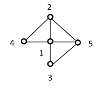
(a) $\{1\},\{2,3\},\{4,5\}$

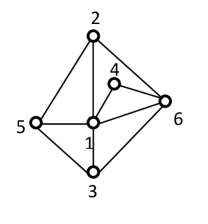
(b) $\{1\},\{2,3,4\},\{5,6\}$

(c) $\{1\},\{2,3,4\},\{5,6\}$

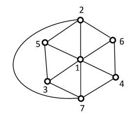
(d) $\{1\},\{2,3,4\},\{5,6,7\}$

Figure 8: A few unstable networks with their unique minimal cover ${\mathcal{M}}^{*}$ using the maximal schedules.

This means any valid covering of $V$ must contain ${\mathcal{M}}^{*}$. Therefore, considering arrival rate vectors of the form $\lambda=\rho\sum_{i=1}^{K^{*}}\sigma_{i}1_{M_{i}}$, $\sigma_{i}>0$, $\sum_{i=1}^{K^{*}}\sigma_{i}=1$, the only way to stabilize the network is to use $M_{i}$ for a time fraction greater than $\rho\sigma_{i}$. Visits to $M_{1}$ have to occur infinitely often, otherwise the network is trivially unstable, and at the end of such visits, a transition to any other maximal schedule is possible, including the schedules in ${\mathcal{M}}\backslash{\mathcal{M}}^{*}$ with positive probability. Then, upon entrance to schedules in ${\mathcal{M}}\backslash{\mathcal{M}}^{*}$, the network spends a positive time in such schedules because the queues in ${\mathcal{M}}\backslash\{M_{1}\}$ build up during visits to $M_{1}$. Hence, the arguments in the instability proof of the broken-diamond network can be extended to such networks, although a rigorous proof of the fluid limits in such general cases remains a formidable task. Figure 8 shows a few examples of such unstable networks with unique minimal set covers.

VII-B Instability for de-activation functions with polynomial decay

Consider any unstable network $G=(V,E)$, for example the broken-diamond network or a graph as described in the previous subsection. Let $\mathcal{I}(i)$ denote the set of neighbors of node $i$ in $G$. We construct a $k$-duplicate graph $G^{(k)}$, $k\in{\mathbb{N}}$, of $G$ as follows. For each node $i\in V$, add $k$ duplicate nodes $d^{(i)}_{1},\dots,d^{(i)}_{k}$ to the graph, with the same arrival rate $\lambda_{i}$ and the same initial queue length $X_{i}(0)$, such that each node $d^{(i)}_{j}$ is connected to all the neighbors of node $i$ and their duplicates, i.e., $\mathcal{I}(d^{(i)}_{j})=\mathcal{I}(i)\cup_{l\in\mathcal{I}(i)}\{d^{(l)}_{1},\cdots,d^{(l)}_{k}\}$, for all $1\leq j\leq k$. For notational convenience, we define $D^{(k)}_{i}:=\{i,d^{(i)}_{1},\dots,d^{(i)}_{k}\}$ and call it the duplicate collection of node $i$. Note that the duplicate graph has the same number of maximal schedules as the original graph. In fact, each maximal schedule $M_{i}^{(k)}$ of $G^{(k)}$ consists of nodes in the maximal schedule $M_{i}$ of $G$ and their duplicates, i.e., $M_{i}^{(k)}=\cup_{l\in M_{i}}D^{(k)}_{l}$. Next, we show that the duplicate graph is unstable for de-activation functions that decay as ${\rm o}(x^{-\gamma})$, for $\gamma>1/(k+1)$. Essentially, for such a range of $\gamma$, each duplicate collection acts as a super node with $\gamma>1$, i.e., (i) if one of the queues in a duplicate collection $D^{(k)}_{i}$ starts growing, all the queues in $D^{(k)}_{i}$ grow linearly at the same rate $\lambda_{i}$ (on the fluid scale), (ii) if a nonempty queue in $D^{(k)}_{i}$ starts draining, then all the queues in $D^{(k)}_{i}$ drain at full rate until they all hit zero (on the fluid scale). Then the instability follows from that of the original network, as we can simply regard the duplicate collections as super nodes. An informal proof of claims (i) and (ii) is presented below.

Claim (i) is easy to prove as all the queues in a duplicate collection share the same set of conflicting neighbors and the fact that one of the queues grows, over a small time interval, implies that some conflicting neighbors are transmitting over such interval. To show (ii), note that if one of the queues in the duplicate collection drains over a non-zero time interval, no matter how small the interval is, all the conflicting neighbors must be in backoff for $O(R)$ units of time in the pre-limit process. This guarantees that all the queues in the duplicate collection will start a packet transmission during such interval almost surely. As long as the duplicate collection does not lose the channel, each queue of the collection follows the fluid limit trajectory of an M/M/1 queue. Suppose all the queues of the duplicate collection are above a level $\epsilon$ on the fluid scale for some fixed small $\epsilon>0$. Thus, in the pre-limit process, the amount of time required for the queues to fall below a threshold $\epsilon R$ is $O(R)$ with high probability as $R\to\infty$. The duplicate collection loses the channel if and only if all $k+1$ nodes in the collection are in backoff and a conflicting node acquires the channel by winning the competition between the backoff timers. The probability that a node goes into backoff at the end of a packet transmission is $O((\epsilon R)^{-\gamma})$, or approximately the fraction of time that a node spends in backoff is $O((\epsilon R)^{-\gamma})$. Therefore, the fraction of time that all $k+1$ nodes of the duplicate collection are simultaneously in backoff is $O((\epsilon R)^{-k\gamma})$ because the nodes in the duplicate collection act independently from each other. Therefore, over an interval of duration $O(R)$, the amount of time that all $k+1$ nodes are in backoff is $O(R^{1-(k+1)\gamma})$, which goes to zero as $R\to\infty$ if $\gamma>1/(k+1)$. Thus, the nodes in the duplicate collection follow the fluid limits of an M/M/1 queue until their backlog is below $\epsilon$ on the fluid scale. Since $\epsilon$ could be made arbitrarily small, we can view the duplicate collection as a super node that does not release the channel until its backlog hits zero. This demonstrates the instability of fluid limits for the initial queue lengths described above for the duplicate network.

To rigorously prove instability of the original process using the framework of Meyn [27], we need to show instability of the fluid limit for any initial state. Handling arbitrary initial states for general activity functions and interference graphs is more involved than in the specific broken-diamond network considered here. An alternative option would be to extend the methodology and develop a proof apparatus where it suffices to show instability of the fluid limit for one particular initial state. The framework of Dai [6] offers the advantage that instability of the fluid limit only needs to be shown for an all-empty initial state. However the characterization of the fluid limit for an all-empty initial state appears to involve additional complications.

The above proof arguments suggest that instability can in fact occur for any $\gamma>0$ as $k$ can be chosen arbitrarily large. This indicates that the growth conditions in Ghaderi & Srikant [15] are sharp in the sense that backoff probabilities of the form $\frac{1}{O(\log(x))}$ are essentially the most aggressive de-activation functions that guarantee maximum stability of queue-based random access in arbitrary graphs. In terms of backoff probabilities $\frac{1}{1+{\rm e}^{w(X)}}$ used in [15], this means the weight functions $w(x)=\log(1+x)/h(x)$, where $h(x)$ is an arbitrarily slowly increasing function, are essentially the most aggressive weight functions that the random-access algorithm can use while preserving maximum stability in general topologies.

Appendix A Fluid limit proofs: Part A

A.I. Prelimit model

We start with the time-homogeneous Markov process $({\bf U}(t),{\bf X}(t)),t\geq 0$ with state space ${\cal S}=S\times{\mathbb{N}}_{0}^{N}$ where $N=6$ and $S\subseteq\left\{0,1\right\}^{N}$ is the set of feasible activity states, which has already been fully described earlier in Section II. We recap to state that service times are unit exponential as are backoff periods. In addition the Poisson arrival processes are determined by the vector of arrival rates $\lambda$ and the probability of backoff is determined as a function of queue length $1/(1+Q)^{\gamma}$ with $\gamma\in(1,\infty)$. As mentioned earlier, the case $\gamma=\infty$ corresponds to the random capture algorithm, considered in [12].

The fluid limit will not be obtained directly from the above process but rather via the jump chain of a uniformized version with “clock ticks” from a Poisson clock with constant rate,

$$\beta\doteq\sum_{\ell=1}^{N}\lambda_{\ell}+N,$$ (9)

independent of state, with null (dummy) events introduced as needed.

With minor abuse of notation, denote by $\left({\bf U}(n),{\bf X}(n)\right)\in{\cal S}$ to be the state of the jump chain at $n$th clock tick. For our subsequent construction, it will be convenient to replace ${\bf U}(n)$ with the cumulative state ${\bf I}(n)=\sum_{k=0}^{n}{\bf U}(n)\in{\mathbb{N}}_{0}^{N}$, which is by definition increasing. It determines and is determined by the sequence ${\bf U}(n)$ and the associated jump chain is Markov if the state is altered to be $({\bf I}(n),{\bf I}(n-1),{\bf X}(n))$ with ${\bf I}(-1)=0$. Note that the process ${\bf I}(n)$ counts the number of steps where the queue process is active. It is not a count of the number of service completions by step $n$.

From the jump chain, we obtain a continuous stochastic process in $C[0,\infty)$ by linear interpolation and by accelerating time by a factor $\beta$. To be specific, at an arbitrary intermediate time $t>0$ between two clock ticks $t_{l}=(k-1)/\beta\leq t\leq t_{u}=k/\beta,~{}k\in{\mathbb{N}}$, the interpolated process takes the values

$$\overline{{\bf Q}}(t) \doteq \beta(t_{u}-t){\bf X}(k-1)+\beta(t-t_{l}){\bf X}(k),$$

$$\overline{{\bf I}}(t) \doteq \beta(t_{u}-t){\bf I}(k-1)+\beta(t-t_{l}){\bf I}(k).$$

From this construction we can obtain a sequence of such processes, indexed by $R\in{\mathbb{N}}$, with the usual fluid limit scaling

$$\left({\bf Q}^{R}(t),{\bf I}^{R}(t)\right)\doteq\left(\frac{1}{R}\overline{{\bf Q}}^{(R)}(Rt),\frac{1}{R}\overline{{\bf I}}^{(R)}(Rt)\right).$$ (10)

This is obtained together with a corresponding sequence of initial queue lengths

$${\bf Q}^{R}(0)=\frac{1}{R}\overline{{\bf Q}}^{(R)}(0)\rightarrow{\bf q}.$$ (11)

Recall that the underlying jump chain $\left({\bf U}(n),{\bf X}(n)\right)_{n\geq 0}$ is affected only through the initial state. Its transition probabilities are unaffected. The convergence in (11) is with respect to the Euclidean norm and without loss of generality we may take $\lvert\lvert{\bf q}\rvert\rvert=1$.

For every $R$ and time $t\geq 0$, $\left({\bf Q}^{R}(t),{\bf I}^{R}(t)\right)$ take values in $E\doteq\mathbb{R}_{+}^{N}\times\mathbb{R}_{+}^{N}$, which is therefore the state space of the process. $E$ has the usual Euclidean metric and associated topology and we will denote the Borel sets by ${\cal B}_{E}$. Furthermore the underlying jump chain $\left({\bf U}(n),{\bf X}(n)\right)_{n\geq 0}$ of the uniformized Markov process satisfies the “skip-free property” [27] which ensures that the jumps between states are bounded in ${\cal L}_{1}$. It follows that the interpolated paths are Lipschitz continuous with Lipschitz constant $3\beta<\infty$. This property is conferred on the sample paths $\omega$ themselves as stated below

$$\lvert\lvert{\bf Q}^{R}(t,\omega)-{\bf Q}^{R}(s,\omega)\rvert\rvert+\lvert\lvert{\bf I}^{R}(t,\omega)-{\bf I}^{R}(s,\omega)\rvert\rvert\leq 3\beta\left(t-s\right)$$ (12)

which holds $\forall\omega,0\leq s<t,R\in{\mathbb{N}}$. The factor 3 appears since at most two queues can be active at the same time and at each clock tick at most one queue can be in(de)cremented.

To summarize, the scaled sequence of processes as defined in (10) take values in the space $C[0,\infty)$ of continuous paths taking values in $E$, endowed with the supnorm topology, and $\sigma$-algebra ${\cal C}$ generated by the open sets. This is obtained through the usual metric $\rho_{C}$ as defined in [40], page 6. This space is both separable and complete, see [40] Theorem 2.1. The probability measure induced on ${\cal C}$ by the $R$th interpolated process (10) is denoted $\mu_{R}$ so that $\mu_{R}(A)$ is the probability of an event $A\in{\cal C}$. Finally, it is of course the case that the jump chain sequence determines and is determined by the corresponding interpolated path. Hence $\mu_{R}$ and the jump chain probabilities are equivalent, given the initial conditions.

A.II. Fluid limit

If there is an infinite subsequence, $R_{k_{1}},R_{k_{2}},\ldots$ such that $\mu_{R_{k_{n}}}\Rightarrow\mu$ where $\Rightarrow$ denotes weak convergence, then $\mu$ is said to be a fluid limit measure. If such a fluid limit exists then the corresponding process can be defined as follows. Its state space is again $E$ with underlying sample space $C[0,\infty)$ and corresponding $\sigma$-algebra ${\cal C}$ generated by the open sets under the metric, $\rho_{C}$, as mentioned earlier. This is the same space as for the sequence of prelimit processes. With the fluid limit measure $\mu$ (including the deterministic initial conditions) we have an underlying probability space $\left(C[0,\infty),{\cal C},\mu\right)$. The stochastic process, $\left({\bf Q},{\bf I}\right)$ is the mapping $[0,\infty)\times C[0,\infty)\rightarrow E$ with values $\left({\bf Q}(t,\omega),{\bf I}(t,\omega)\right)\in E$. The curves $\left({\bf Q}(.,\omega),{\bf I}(.,\omega)\right)$ and $\omega$ itself are the same. Whilst these definitions are somewhat redundant, nevertheless in what follows, it will be convenient to think of a sample path as either a point $\omega$ or as a random function. Finally, on some occasions, we will use the notation $X\in m{\cal C}$ to indicate that $X:C[0,\infty)\rightarrow\mathbb{R}$ is measurable.

The proof of the next Theorem is standard and follows from Lipschitz continuity, Theorem 8.3 of [1], and Lemma 3.1 of [40]. The details are omitted for brevity.

Theorem 4

The sequence of measures $\mu_{R}$ defined on $\left(C[0,\infty),{\cal C}\right)$ is tight.

Thus, it follows from Prohorov’s Theorem (Theorem 6.1 of [1]) that the sequence $\mu_{R}$ is relatively compact and fluid limit measure $\mu$ must exist. We suppose without loss of generality that $\mu_{R}\Rightarrow\mu$. The sample paths under $\mu$ have the same Lipschitz constant $3\beta$. It follows that the sample paths of $\mu$ are differentiable a.e., almost surely [32].

Lipschitz continuity also implies that there are only a countable number of closed intervals $[a,b]$, $0\leq a<b$, such that $Q_{\ell}(a,\omega)=Q_{\ell}(b,\omega)=0$, $\ell=1,\cdots,N$, and $Q_{\ell}(x,\omega)>0,\forall x\in(a,b)$, $\ell=1,\cdots,N$, holding almost surely.

We denote by $\left\{{\cal F}_{t}\right\}_{t\in[0,\infty)},~{}{\cal F}_{t}\subset{\cal C}$, the filtration of sub $\sigma$-algebras generated by the open sets restricted to the interval $[0,t]$. The process $\left({\bf Q},{\bf I}\right)$ is adapted to $\left\{{\cal F}_{t}\right\}_{t\in[0,\infty)}$ (In fact it is ${\cal F}_{t}$-progressive as the process is continuous, see [10]).

By consideration of the weak law of large numbers and the existence of the fluid limit measure $\mu$, it holds that

$${\bf Q}(t)={\bf Q}(0)+\mbox{\boldmath$\lambda$}t-\frac{1}{\beta}{\bf I}(t),~{}t\geq 0.$$ (13)

This equation can be thought of as an accounting identity. If queue $\ell$ is active for a unit interval then $I_{\ell}$ increases by $\beta$, which corresponds (almost surely) to departures at unit rate. During the same period the arrival rate is $\lambda_{\ell}$ of course.

Since $I_{\ell}(t+h)-I_{\ell}(t)\leq\beta h$ for any node $\ell$, and any times $t\geq 0$ and $h>0$, it follows from (13) that

$$Q_{\ell}(t+h)\geq Q_{\ell}(t)+\lambda_{\ell}h-h,~{}\mu~{}a.s.$$ (14)

We now derive an elementary property of the fluid limit process. Given $t\geq 0,h>0$, define

$$Y^{\ell}_{t,h}\doteq\left\{\omega:I_{\ell}(t+h,\omega)-I_{\ell}(t,\omega)=\beta h\right\}$$ (15)

to be the event that queue $\ell$ is being served (at maximum rate) during the interval $[t,t+h]$, i.e., the node is fully active during the given interval. Since many of the events that we consider later are in terms of activity, we adapt the following notation throughout the paper. In the case of (15),

$$Y^{\ell}_{t,h}=J^{(\ell)}_{=}(t,h,\beta h)$$ (16)

where the superscript “$\ell$” denotes the node, “$t$” time and “$h$” duration. “$\beta h$” is the amount of activity which must be met with equality here, as indicated by the subscript “=”. The subscript “=” may be replaced by $>$, $\geq$, $<$, or $\leq$, depending on the event.

Lemma 3 (No Conflict Lemma)

Let $\ell_{1}\neq\ell_{2}\in\left\{1,\cdots,N\right\}$ be two neighbors in the interference graph $G$, and $h>0,t\geq 0$, then

$$\mu\left\{Y^{\ell_{1}}_{t,h}\cap Y^{\ell_{2}}_{t,h}\right\}=0.$$ (17)

Proof:

This follows by definition, and the existence of the fluid limit. The event $Y^{\ell_{1}}_{t,h}\cap Y^{\ell_{2}}_{t,h}$ contradicts the inequality that for all $t\geq 0,h>0$,

$$\left[I_{\ell_{1}}(t+h,\omega)-I_{\ell_{1}}(t,\omega)\right]+\left[I_{\ell_{2}}(t+h,\omega)-I_{\ell_{2}}(t,\omega)\right]\leq\beta h,$$

which holds $\mu$ almost surely. ∎

To obtain more detailed information with respect to the sample paths of $\mu$, we proceed to the construction of sequences of stopping times.

A.III. Sequences of stopping times

The following definition is in connection with the amount of time a sample path for $Q_{\ell}$ is positive, immediately prior to a time $z>0$.

Definition 2

Given a time $z>0$, and $v,0<v\leq z$, and an $\ell=1,\cdots,N$, define

$$K^{(\ell)}_{z,v}\doteq\left\{\omega:Q_{\ell}(z-s,\omega)>0,~{}\forall s\in(0,v)\right\}.$$

In words, $K^{(\ell)}_{z,v}$ is the set of sample paths for $Q_{\ell}$ which are strictly positive in the interval $(z-v,z)$; if $z=0$, $K^{(\ell)}_{z,v}$ is taken to be $\emptyset$.

Observe that it could be the case that either $Q_{\ell}(z,\omega)=0$ or $Q_{\ell}(z-v,\omega)=0$ (or both) and still $\omega\in K^{(\ell)}_{z,v}$. Finally note that it is possible for a given $\omega$ that no such $v$ can be found, which requires that $Q_{\ell}(z,\omega)=0$ on account of continuity. It can be shown that

$$K^{(\ell)}_{z,v}=\cap_{n:2/n<v}\left[\cup_{m=1}^{\infty}\left\{\omega:Q_{\ell}(z-q,\omega)\geq 1/m,~{}q\in[1/n,v-1/n]\cap{\mathbb{Q}}\right\}\right]\in{\cal F}_{z},$$

for $z>0$, where ${\mathbb{Q}}$ is the set of rational numbers.

Given a time $z\geq 0$ and a path $\omega$, we define the mapping $A^{(\ell)}(z,\omega):C[0,\infty)\rightarrow[0,z]$ to be $A^{(\ell)}(z,\omega)\doteq\sup\left[\left\{v:\omega\in K^{(\ell)}_{z,v}\right\}\cup\left\{0\right\}\right]$, which is the time for which $Q_{\ell}$ was positive immediately prior to $z$. By definition, if $z\geq u>0$ then

$$\left\{\omega:A^{(\ell)}(z,\omega)\geq u\right\}=K^{(\ell)}_{z,u},$$

from which it follows that $A^{(\ell)}(z,\omega)\in m{\cal F}_{z}$. So far $z$ has been fixed. However $A^{(\ell)}:[0,\infty)\times C[0,\infty)\rightarrow\mathbb{R}_{+}$ is a stochastic process carried by the underlying probability space $\left(C[0,\infty),{\cal C},\mu\right)$ and ${\cal F}_{t}$-adapted as we have just seen. This process is piecewise linear and left-continuous (It falls to 0 immediately after $Q_{\ell}$ returns to 0 from being positive). It follows that $A^{(\ell)}$ is ${\cal F}_{t}$-progressive, see for example [10]. We are now in a position to make the following definition.

Definition 3

Given an ${\cal F}_{t}$ stopping time $\sigma$, a queue $\ell\in 1,\cdots,N$ and $m\in{\mathbb{Z}}_{0}\doteq{\mathbb{Z}}-\left\{0\right\}$, define $T_{\ell,m}(\omega,\sigma):C[0,\infty)\times[0,\infty]\rightarrow[0,\infty]$ as follows

$$T_{\ell,m}(\omega,\sigma)\doteq\inf\left\{z\geq\sigma(\omega):Q_{\ell}(z)=0,A^{(\ell)}(z,\omega)\in(e_{m},f_{m}]\right\}\leq\infty,$$

where

$$f_{m} = \frac{1}{m},~{}e_{m}=\frac{1}{m+1};\mbox{ for }m\in{\mathbb{Z}}_{0},~{}m>0,$$

$$f_{m} = \lvert{m-1}\rvert,~{}e_{m}=\lvert{m}\rvert;\mbox{ for }m\in{\mathbb{Z}}_{0},~{}m<0,$$

where again empty sets have an infinite infimum.

In words, $T_{\ell,m}$ is the earliest right-hand end of an open interval, with value $z$, such that $Q_{\ell}$ is positive for a period $A^{(\ell)}(z,\omega)\in(e_{m},f_{m}]$, immediately prior to $T_{\ell,m}$. If $z-f_{m}$ is the first time prior to $z$ that $Q_{\ell}=0$, then $z$ is in the set on the RHS. However, if this occurs at $z-e_{m}$, this is not the case.

It is plausible that $T_{\ell,m}$ is also an ${\cal F}_{t}$ stopping time, and we will subsequently prove this with particular choices for $\sigma$. We now state a construction lemma using a sequence of stopping times. These are returns to 0 following a fixed positive interval, in which we wait for a particular event $A_{k}$ to occur.

Lemma 4 (Stop and Look Back)

Let $\sigma\geq 0$ be an ${\cal F}_{t}$ stopping time and $a>0$ a constant. Proposition 1.5 in Ethier & Kurtz [10] ensures that the following inductively defined sequence is a sequence of ${\cal F}_{t}$ stopping times: $s_{0},s_{1},s_{2},\ldots$,

$$s_{0} \doteq \sigma$$ (18)

$$s_{k} \doteq \tau_{c}(\left\{0\right\},s_{k-1}+a),~{}k=1,2,\cdots$$

Here, given an ${\cal F}_{t}$ stopping time $\sigma_{1}>0$, $\tau_{c}(\left\{0\right\},\sigma_{1})=\inf\left\{t\geq\sigma_{1},Q(t,\omega)=0\right\}$. Now let $A_{k}\in{\cal F}_{s_{k}},k=1,2,\ldots$ be a sequence of events in the pre-$T$ $\sigma$-algebras of the above stopping time sequence. Finally, define $\tau\doteq s_{k}$ if $A_{k}$ occurs for the first time at step $k$ and $\tau=\infty$ otherwise. Then $\tau$ is an ${\cal F}_{t}$ stopping time.

Note that we do not check to see if $A_{k}$ has occurred if $s_{k}=\infty$ at any stage, as $\tau$ is assigned this value regardless.

We now proceed to show the following.

Lemma 5

Let $\sigma_{0}\geq 0$ be an ${\cal F}_{t}$ stopping time such that $Q_{\ell}(\sigma_{0}(\omega),\omega)=0$ or $\sigma_{0}=\infty$ and suppose $\ell,m$ are given. Let $a=e_{m}$ and $\sigma\doteq a+\sigma_{0}$ which is therefore an ${\cal F}_{t}$ stopping time, and $T_{\ell,m}$ be the mapping given in Definition 3. Then $T_{\ell,m}(\omega,\sigma)$ is an ${\cal F}_{t}$ stopping time.

Proof:

Given $\sigma$ we will obtain a sequence of stopping times as in the first part of Lemma 4. However as we have already discussed, $A^{(\ell)}$ is ${\cal F}_{t}$-progressive, from which it follows by Proposition 1.4 of [10] that

$$A_{k}:=A^{(\ell)}(s_{k}(\omega),\omega)\in m{\cal F}_{s_{k}},\forall~{}k=1,2,3,\ldots$$

so that $A^{(\ell)}(s_{k}(\omega),\omega)\in(e_{m},f_{m}]\in{\cal F}_{s_{k}}$. Hence $\tau$ as defined in Lemma 4 is an ${\cal F}_{t}$ stopping time.

It remains to show that $\tau$ coincides with $T_{\ell,m}$ as defined. First suppose $\tau<\infty$, and immediately, $\tau\geq\sigma,Q_{\ell}(\tau,\omega)=0,A^{(\ell)}(\tau,\omega)\in(e_{m},f_{m}]$ by definition. The fact that there is no earlier time satisfying these conditions follows since each $s_{k}$ is a zero of $Q_{\ell}$ and the construction rules out that the event could have taken place any earlier. The case $\tau=\infty$ coincides with there being no zero satisfying the required conditions. ∎

We now make the following recursive definitions.

Definition 4

Given $m\in{\mathbb{Z}}_{0}$ and queue $\ell\in\left\{1,\cdots,N\right\}$, let $\tau_{0}$ be the first entry of $Q_{\ell}(t,\omega)$ into 0 ($\tau_{0}$ is an ${\cal F}_{t}$ stopping time). Then $Z^{\ell}_{m,0}$ is defined as

$$Z^{\ell}_{m,0} \doteq T_{\ell,m}(\omega,0);\mbox{ if $Q_{\ell}(0,\omega)=0$}$$

$$Z^{\ell}_{m,0} \doteq \tau_{0};\mbox{ if $Q_{\ell}(0,\omega)>0$, $\tau_{0}\in(e_{m},f_{m}]$}$$

$$Z^{\ell}_{m,0} \doteq T_{\ell,m}(\omega,\tau_{0});\mbox{ if $Q_{\ell}(0,\omega)>0$, $\tau_{0}\notin(e_{m},f_{m}]$},$$

and subsequent stopping times are defined as

$$Z^{\ell}_{m,n}\doteq T_{\ell,m}(\omega,Z^{\ell}_{m,n-1}),~{}n=1,2,3,\ldots.$$

The value of the stopping time is taken to be $\infty$ if the events do not occur. With obvious notation, we also define

$$A^{\ell}_{m,n}(\omega)\doteq A^{(\ell)}(Z^{\ell}_{m,n},\omega)$$

to be the actual amount of time that the queue $\ell$ is positive prior to $Z^{\ell}_{m,n}$, and $A^{\ell}_{m,n}=\infty$ in case $Z^{\ell}_{m,n}=\infty$. Finally define the time at which $Q_{\ell}$ last enters $(0,\infty)$ prior to $Z^{\ell}_{m,n}$ to be

$$V^{\ell}_{m,n}\doteq Z^{\ell}_{m,n}-A^{\ell}_{m,n},$$

when $Z^{\ell}_{m,n}<\infty$ and $V^{\ell}_{m,n}=\infty$ otherwise. Note that $V^{\ell}_{m,n}\in m{\cal F}_{Z^{\ell}_{m,n}}$ and is thus a non-negative random variable but not a stopping time.

The following corollary follows immediately from Lemma 5 and Definition 4.

Corollary 2

$Z^{\ell}_{m,n},n\in{\mathbb{N}}_{0}$ is a strictly increasing sequence of ${\cal F}_{t}$ stopping times, $\forall\ell\in N,m\in{\mathbb{Z}}_{0}$.

This completes our goal of constructing sequences of stopping times for the queue processes. For any queue $\ell$, by construction and by Lipschitz continuity, it follows that the set of stopping times, $Z^{\ell}_{m,n}$ determine all intervals where $Q_{\ell}$ is positive for any sample path almost surely.

For each $m\in{\mathbb{Z}}_{0}$, and $\ell\in\left\{1,\cdots,N\right\}$, define

$$B^{\ell}_{m}\doteq\sup_{n}\left\{Z^{\ell}_{m,n}:Z^{\ell}_{m,n}<\infty\right\}$$

to be the supremum of the finite stopping times for positive intervals with duration in $(e_{m},f_{m}]$. If there is an $m$ such that $B^{\ell}_{m}=\infty$, then $Q_{\ell}$ returns to 0 infinitely often. Otherwise there is a $B>0,B>B^{\ell}_{m},\forall m\in{\mathbb{Z}}_{0}$. In this case, either $Q_{\ell}$ remains at 0 as $t\rightarrow\infty$, or queue $\ell$ never returns to 0.

A.IV. Piecewise linearity and no backoff until empty

So far the backoff exponent $\gamma>1$ has not been taken into consideration, but from now on it will be. The following lemma bounds the probability, for the jump chain, that node $\ell$ has a backoff before its queue gets “small” provided that it was active earlier. Given some number $X_{T}\in{\mathbb{N}}$ define,

$$K_{X_{T}}\doteq\left\{\exists n:X_{\ell}(k)\geq X_{T},0\leq k\leq n,U_{\ell}(n)=0,U_{\ell}(n-1)=1\right\}$$

to be the event that queue $\ell$ has remained above $Q_{T}$ and has had a backoff at step $n$. We then have the following lemma,

Lemma 6 (No Early Backoff)

Given any $X_{0}>X_{T}$,

$${\mathbb{P}}\{K_{X_{T}}|X_{\ell}(0)\geq X_{0}\}\leq\frac{1}{1-\lambda_{\ell}}\times\sum_{r=X_{T}}^{\infty}\frac{1}{(1+r)^{\gamma}}=\varepsilon_{X_{T}}.$$ (19)

Since the sum is convergent, $\varepsilon_{X_{T}}\downarrow 0$ as $X_{T}\uparrow\infty$.

Proof:

It is convenient to consider the packets being served in generations. That is given a target packet, suppose that we serve the packets which arrive during its service with preemptive priority up to and including the target packet. This makes no difference to queue behaviour as the service times are exponential and we are only interested in the first occasion when node $\ell$ goes into backoff.

Suppose there are $X_{T}>0$ packets in queue at the time the service of a given target packet starts. Consider the busy period of this packet, i.e. the time to serve the target packet and the subsequent high-priority packets (without backoff). It is easy to see that the mean number of packet arrivals during this busy period is $\frac{1}{1-\lambda_{\ell}}$, including the target packet itself.

The service of each packet ends with a random decision to backoff with probability less than $\frac{1}{\left(1+X_{T}\right)^{\gamma}}$, since the queue length is never shorter than $X_{T}$ until the target packet has departed. Thus, by the union bound, the probability of a backoff occurring before or immediately after the target packet departs, is less than $\frac{1}{\left(1+X_{T}\right)^{\gamma}}\times\frac{1}{1-\lambda_{\ell}}$. The probability of a backoff, starting with $X_{0}>X_{T}$ packets, and before the queue drops below the level $X_{T}$, is therefore smaller than $\frac{1}{1-\lambda_{\ell}}\sum_{r=X_{T}}^{r=X_{0}}\frac{1}{(1+r)^{\gamma}}$ which implies the statement of Lemma.

∎

The following lemma will also be useful. First given times $t_{2}>t_{1}\geq 0$ on the fluid scale, let $B_{\ell}([t_{1},t_{2}])$ be the event that node $\ell$ starts a backoff in the interval $[t_{1},t_{2}]$. This event occurs in the prelimit process $\left(Q^{R}_{\ell},I^{R}_{\ell}\right)$ if for some jump chain index $n,U_{\ell}(n)=1,U_{\ell}(n+1)=0$ with $\lfloor Rt_{1}\beta\rfloor\leq n\leq\lceil Rt_{2}\beta\rceil$. Let $D_{\ell,\varsigma}([t_{1},t_{2}])$be the event that $Q^{R}_{\ell}(u)>\varsigma$ (or equivalently $\bar{Q}_{\ell}(Ru)\geq R\varsigma$) for all $u$ in the interval $[t_{1},t_{2}]$.

Lemma 7

Given the above definitions,

$$\lim_{R\rightarrow\infty}\mu_{R}\left\{B_{\ell}{[t_{1},t_{2}]}\cap D_{\ell,\varsigma}([t_{1},t_{2}])\right\}=0$$ (20)

Proof:

First we may suppose node $\ell$ becomes active at some stage or there is nothing to prove. The lemma then follows from the union bound. Since there are at most $R_{t_{1},t_{2}}\doteq\lceil R(t_{2}-t_{1})\beta\rceil+2$ departures in the entire interval, the union bound implies that the probability of a backoff is smaller than,

$$\mu_{R}\left\{B_{\ell}{[t_{1},t_{2}]}\cap D_{\ell,\varsigma}([t_{1},t_{2}])\right\}\leq\frac{R_{t_{1},t_{2}}}{\left(1+R\varsigma\right)^{\gamma}}\rightarrow 0.$$

This completes the proof. ∎

Definition 5

Given a queue $\ell$, a time $t\in[0,\infty)$ on the fluid scale, and a queue length $Q_{\ell}(t)=Q>0$, we say that $t$ is a point of increase for the activity process of queue $\ell$ if the event

$$P_{t,Q}^{(\ell)}\doteq\cap_{M=1}^{\infty}\left\{J^{(\ell)}_{>}(t,\frac{1}{M},0)\right\}\cap Q^{(\ell)}_{t,Q}$$

occurs, with $Q^{(\ell)}_{t,Q}\doteq\left\{\omega:Q_{\ell}(t,\omega)>Q\right\}$. In words, queue $\ell$ is active in any arbitrarily small interval $(t,t+1/M)$ and $Q_{\ell}$ is greater than $Q$ at time $t$.

Furthermore, given a time $s\in[0,\infty)$ and $h>0$, we say that queue $\ell$ is under active, with duration $h>0$ if the following event occurs

$$G^{(\ell)}_{s,h}\doteq J^{(\ell)}_{<}(s,h,\beta h).$$ (21)

Points of increase rule out that there is a sequence $t_{n}\downarrow t$ such that $I_{\ell}(t_{n},\omega)=I_{\ell}(t,\omega)$, as there is activity no matter how small the interval. Under activity means that there was some idling during the interval. Given our choice of $\gamma$, it will be shown that a point of increase cannot be followed by a period of under activity until queue $Q_{\ell}$ has drained. This is because the probability of even a single backoff once service has begun, is effectively 0 until the queue has drained on the fluid scale.

Lemma 8

Suppose $s\in\left(t,t+Q/(1-\lambda_{\ell})\right)$. Then $\forall h,0<h<t+Q/(1-\lambda_{\ell})-s$, and for all sufficiently large $M$,

$$\mu\left\{J^{(\ell)}_{>}(t,1/M,0)\cap Q^{(\ell)}_{t,Q}\cap G^{(\ell)}_{s,h}\right\}=0.$$ (22)

Proof:

Consider the sequence of prelimit processes. We will choose $M$ large enough and $\varsigma$ small enough so that $[s,s+h]\subset(t+1/M,t+(Q-\varsigma)/(1-\lambda_{\ell})]$ (for some small constant $\varsigma>0$). Then for $R,M$ sufficiently large, and then by definition, occurrence of $G^{(\ell)}_{s,h}$, for the $R$-th prelimit process, implies occurrence of $B_{\ell}([t+1/M,s+h])$. Hence we obtain,

$$\mu_{R}\left\{J^{(\ell)}_{>}(t,1/M,0)\cap Q^{(\ell)}_{t,Q}\cap G^{(\ell)}_{s,h}\right\} \leq \mu_{R}\left\{J^{(\ell)}_{>}(t,1/M,0)\cap Q^{(\ell)}_{t,Q}\cap B_{\ell}([t+1/M,s+h])\right\}$$

$$\leq \mu_{B,R}+\mu_{F,D,R},$$

where

$$\mu_{B,R}\doteq\mu_{R}\left\{J^{(\ell)}_{>}(t,1/M,0)\cap B^{(\ell)}\left(t+1/M,s+h\right)\cap D_{\ell,\varsigma}([t,s+h])\right\},$$ (24)

and

$$\mu_{F,D,R}\doteq\mu_{R}\left\{Q^{(\ell)}_{t,Q}\cap\left(D_{\ell,\varsigma}([t,s+h])\right)^{c}\right\}.$$ (25)

Thus, in order to prove the lemma, it is sufficient to show that both $\mu_{B,R}\rightarrow 0$ and $\mu_{F,D,R}\rightarrow 0,$ as $R\rightarrow\infty$, because then we may conclude that

$$\mu\left\{J^{(\ell)}_{>}(t,1/M,0)\cap Q^{(\ell)}_{t,Q}\cap G^{(\ell)}_{s,h}\right\}\leq\liminf\mu_{R}\left\{J^{(\ell)}_{>}(t,1/M,0)\cap Q^{(\ell)}_{t,Q}\cap G^{(\ell)}_{s,h}\right\}=0$$

on applying Theorem 2.1 in [1] and since the sets $J^{(\ell)}_{>}(t,1/M,0),Q^{(\ell)}_{t,Q},G^{(\ell)}_{s,h}$ are all open.

The fact that $\mu_{F,D,R}\rightarrow 0$ follows from (13) and then by definition of $Q^{(\ell)}_{t,Q}$ and additionally by the choice of $s,h,\varsigma$. As far as $\mu_{B,R}$ is concerned, the event $J^{(\ell)}_{>}(t,1/M,0)$ implies that service has started during the interval $[t,t+1/M]$. On the other hand, the event $B_{\ell}([t+1/M,s+h])$ implies that at some time in $[t,s+h]$ node $\ell$ starts to backoff. Setting $t_{1}=t$ and $t_{2}=s+h$, we may invoke Lemma 7 as by definition the event $D_{\ell,\varsigma}([t,s+h])$ implies $Q_{\ell}$ did not go below $\varsigma$ in the interval $[t_{1},t_{2}]$. It follows that $\mu_{B,R}\rightarrow 0$ as required. ∎

The implication of Lemma 8 is that any positive period of transmission, no matter how short, must be followed by full activity until the queue has drained on the fluid scale. This implies that there is no period of under activity, until the queue has drained, with probability 1.

A.V. Piecewise linear paths with probability 1

The aim of this section is to show that the queue sample paths follow a certain bilinear path during the interval prior to the queue becoming zero again. The bilinear path depends on the duration of the interval and on the arrival rate for the given queue.

To make the above statements precise, given $\ell\in\left\{1,\cdots,N\right\}$ define the bilinear path $\Phi^{\ell}_{t_{0},t_{1}}$ for the interval $[t_{0},t_{1}]$ to be,

$$\Phi^{\ell}_{t_{0},t_{1}}(s)=\left\{\begin{array}[]{ll}\lambda_{\ell}\left(s-t_{0}\right);&t_{0}\leq s\leq s_{0},\\ \lambda_{\ell}\left(s-t_{0}\right)-(1-\lambda_{\ell})(s-s_{0});&s_{0}\leq s\leq t_{1},\end{array}\right.$$ (28)

where $s_{0}\doteq t_{1}-\lambda_{\ell}(t_{1}-t_{0})$. In words, $Q_{\ell}$ builds up linearly in the interval $[t_{0},s_{0}]$ at rate $\lambda_{\ell}$ and drains at rate $1-\lambda_{\ell}$ in the interval $[s_{0},t_{1}]$.

Given $\eta>0$, and $\ell\in\left\{1,\cdots,N\right\}$, define ${\rm 1\rule{0.43057pt}{6.54443pt}\hskip 0.86108pt}_{t_{0},t_{1}}^{(\eta,\ell)}$ to be the indicator for the event

$$\left\{\omega:\sup_{s\in[t_{0},t_{1}]}\lvert{Q_{\ell}(s,\omega)-\Phi^{\ell}_{t_{0},t_{1}}(s)}\rvert<\eta\right\}\in{\cal F}_{t_{1}}$$

In words, ${\rm 1\rule{0.43057pt}{6.54443pt}\hskip 0.86108pt}_{t_{0},t_{1}}^{(\eta,\ell)}(\omega)=1$ iff the absolute difference between $\Phi^{\ell}_{t_{0},t_{1}}$ and the sample path for $Q_{\ell}$ is smaller than $\eta$ in supnorm over the interval $[t_{0},t_{1}]$.

We now examine the conditional probability that ${\rm 1\rule{0.43057pt}{6.54443pt}\hskip 0.86108pt}_{V^{\ell}_{m,n},Z^{\ell}_{m,n}}^{(\eta,\ell)}(\omega)=1$, given $Z^{\ell}_{m,n}<\infty$ and $A^{\ell}_{m,n}$ (the case $Z^{\ell}_{m,n}=\infty$ is irrelevant). Define, ${\cal Z}^{\ell}_{m,n}\doteq\sigma\left(Z^{\ell}_{m,n},A^{\ell}_{m,n}\right)\subset{\cal C}$ and also ${\cal Z}^{\ell,\infty}_{m,n}={\cal Z}^{\ell}_{m,n}\cap\left\{\omega:Z^{\ell}_{m,n}(\omega)<\infty\right\}$.

It will be enough to show that the sample paths lie in an arbitrarily small tube around $\Phi^{\ell}_{V^{\ell}_{m,n},Z^{\ell}_{m,n}}$ conditional on $A^{\ell}_{m,n},Z^{\ell}_{m,n}$ lying in some small rectangle $Z_{(s,t)}^{(a,b)}\doteq\left\{\omega:A^{\ell}_{m,n}(\omega)\in(a,b],Z^{\ell}_{m,n}(\omega)\in(s,t]\right\}\in{\cal Z}^{\ell,\infty}_{m,n}$.

Theorem 5

Given $n\geq 1,m\in{\mathbb{Z}}_{0}$, then $\forall\eta>0$,

$$\mu\left\{{\rm 1\rule{0.43057pt}{6.54443pt}\hskip 0.86108pt}_{V^{\ell}_{m,n},Z^{\ell}_{m,n}}^{(\eta,\ell)}=1|{\cal Z}^{\ell,\infty}_{m,n}\right\}=1~{}a.s.$$ (29)

In words, given the stopping time $Z^{\ell}_{m,n}$ and the time prior to this that $Q_{\ell}$ was positive, $A^{\ell}_{m,n}$, the probability that $\Phi^{\ell}_{V^{\ell}_{m,n},Z^{\ell}_{m,n}}$ is followed, starting at $V^{\ell}_{m,n}$ and ending at $Z^{\ell}_{m,n}$, is 1 under the fluid limit measure $\mu$.

Proof:

For any given $\varepsilon>0$, the sets $Z_{(s,t)}^{(a,b)}$ $0<s<t$, $0<a<b$, $0<t-s,b-a<\varepsilon$, are a $\pi$-system [2] (i.e. closed under finite intersections) and which generate ${\cal Z}^{\ell,\infty}_{m,n}$. Hence we only need to show that

$$\mu\left\{{\rm 1\rule{0.43057pt}{6.54443pt}\hskip 0.86108pt}_{V^{\ell}_{m,n},Z^{\ell}_{m,n}}^{(\eta,\ell)}(\omega)=1;Z_{(s,t)}^{(a,b)}\right\}=\mu\left\{Z_{(s,t)}^{(a,b)}\right\},$$

for suitably chosen $\varepsilon$ given $\eta>0$.

Let $B^{\ell}_{m,n}(\omega)\leq A^{\ell}_{m,n}$ be the additional time, following strict entry of $Q_{\ell}$ into $(0,\infty)$ at $V^{\ell}_{m,n}$, until the first point of increase of $I_{\ell}$ is reached. $B^{\ell}_{m,n}\in m{\cal F}_{Z^{\ell}_{m,n}}$ as can be seen on consideration of its definition,

$$B^{\ell}_{m,n}(\omega)\doteq\inf\left\{u\in(0,A^{\ell}_{m,n}(\omega))\cap{\mathbb{Q}}~{}:I_{\ell}(V^{\ell}_{m,n}+u,\omega)-I_{\ell}(V^{\ell}_{m,n},\omega)>0\right\},$$ (30)

when $Z^{\ell}_{m,n}<\infty$.

By definition of $B^{\ell}_{m,n}$, Lemma 8 and then (13), we may deduce that for $\omega\in Z_{(s,t)}^{(a,b)}$

$$Q_{\ell}(V^{\ell}_{m,n}(\omega)+u,\omega) = \lambda_{\ell}u,~{}u\in[0,B^{\ell}_{m,n}(\omega)],$$ (31)

$$Q_{\ell}(V^{\ell}_{m,n}(\omega)+u,\omega) = \lambda_{\ell}B^{\ell}_{m,n}(\omega)-(1-\lambda_{\ell})(u-B^{\ell}_{m,n}),~{}u\in[B^{\ell}_{m,n}(\omega),\frac{B^{\ell}_{m,n}(\omega)}{1-\lambda_{\ell}}],$$

$\mu$ almost surely. Moreover $B^{\ell}_{m,n}(\omega)$ must satisfy

$$t-s+b\geq\frac{B^{\ell}_{m,n}(\omega)}{1-\lambda_{\ell}}\geq s-t+a,~{}\mu~{}a.s.$$

in order to reach 0 in $[s,t]$.

Therefore, given any $\eta>0$, we may choose $\varepsilon_{\eta}>0$ such that for all $v\in[s-b,t-a],z\in[s,t]$ with $b-a,t-s<\varepsilon_{\eta}$

$$\sup_{u\in[v,z]}\lvert{Q_{\ell}(u,\omega)-\Phi^{\ell}_{v,z}(u)}\rvert<\eta,$$

$\mu$ almost surely, using Lipschitz continuity. Since $\omega\in Z^{(a,b)}_{(s,t)}$ implies $V^{\ell}_{m,n}\in[s-b,t-a],Z^{\ell}_{m,n}\in[s,t]$, we obtain that

$$\mu\left\{{\rm 1\rule{0.43057pt}{6.54443pt}\hskip 0.86108pt}_{V^{\ell}_{m,n},Z^{\ell}_{m,n}}^{(\eta,\ell)}(\omega)=1;Z_{(s,t)}^{(a,b)}\right\}=\mu\left\{Z_{(s,t)}^{(a,b)}\right\},$$

for all such $a,b,s,t$ as required. ∎

A similar result can be obtained when $n=0$, where the possibility occurs that $Q_{\ell}(V^{\ell}_{m,0})>0$.

A.VI. Brief discussion of results

Theorem 5 applies to general networks and relies only on the assumption that $\gamma>1$. The theorem implies that the sample paths are more or less determined given the sequences of stopping times $Z^{\ell}_{m,n}$. Only in the case where the (finite) stopping times have a common upper bound is the process not completely defined, as otherwise the queue returns to 0 infinitely often, determining the path completely. If there is such a bound, either the queue remains at 0, or increases linearly, as there can be no subsequent point of increase of $I_{\ell}$.

Indeed, since there are only countably many stopping times, and since for each finite $Z^{\ell}_{m,n}<\infty$ the queue sample paths follow $\Phi^{\ell}_{.,.}$ for some finite interval with probability 1, we may confine sample path realizations to countable successions of such intervals. These either determine the entire sample path; or the queue remains at 0 following the final return; or as the final alternative, the queue remains zero for some interval and then increases linearly at rate $\lambda_{\ell}$ thereafter. We define the set of such sample paths by $P\subset C[0,\infty)$. The probability of any event $F\in{\cal C}$ can as well be taken as

$$\mu\left\{F\right\}=\mu\left\{F\cap P\right\},$$

and, therefore, we suppose that the probability space is defined on ($P,{\cal C}_{P}$) with topology relativized in the usual way to $P$ which is a subset of ${\cal C}[0,\infty)$. This establishes that the queue-length trajectory of each of the individual nodes exhibits sawtooth behavior in the fluid limit. This concludes Part A.

In Part B, we will show that we can in fact confine ourselves to a smaller set of paths which reflect the constraints resulting from the underlying interference graph.

Appendix B Fluid limit proofs: Part B

B.I. No idling property and zero delay capture

From Lemma 3, it follows that if queue 2 is draining, then queues 3, 4, 5, 6 are increasing linearly. However, we also expect that queue 1 is either draining or remaining at 0 until time $t$, and this is indeed the case as we now show.

More generally, given a node $\ell$, let ${\cal I}_{\ell}$ be the set of its interfering nodes, i.e. the set of its neighbors in the interference graph $G$. The following lemma shows that if $Q_{\ell}(s)>Q$, and all its interferers are idle in some interval $[s,t]$ then node $\ell$ is fully active until its queue drains.

Lemma 9 (No Idling Property)

Given a node $\ell$ with interference set ${\cal I}_{\ell}$ and an interval $[s,t]$, define

$$D^{(\ell)}_{s,t}\doteq\cap_{j\in{{\cal I}_{\ell}}}J^{(j)}_{=}(s,t-s,0),$$

that is, no activity for any node in ${\cal I}_{\ell}$ during $[s,t]$. Further, given $Q>0$, define $h^{(\ell)}_{s,t,Q}\doteq Q/(1-\lambda_{\ell})\wedge(t-s)$ so that the queue at most empties over this period, and let

$$S^{(\ell)}_{s,t}\doteq J^{(\ell)}_{<}(s,h^{(\ell)}_{s,t,Q},\beta h^{(\ell)}_{s,t,Q}),$$

which implies that node $\ell$ is under active. Then

$$\mu\left\{D^{(\ell)}_{s,t}\cap S^{(\ell)}_{s,t}\cap Q^{(\ell)}_{s,Q}\right\}=0,$$

where $Q^{(\ell)}_{s,Q}$ is the event $\left\{\omega:Q_{\ell}(s,\omega)>Q\right\}$, as defined earlier.

Proof:

Given $n\in{\mathbb{N}}$ such that $n>1/(t-s)$, fix an arbitrary $\zeta,$ $0<\zeta<\frac{1}{2N}$ (Recall that $N$ is the number of nodes in the network). Clearly,

$$D^{(\ell)}_{s,t}\subset\tilde{D}^{(\ell)}_{\zeta,n}:=\cap_{j\in{\cal I}_{\ell}}J^{(j)}_{<}(s,1/n,\zeta/n).$$

Hence, for arbitrary $\epsilon_{n}>0$ depending on $n$, to be fixed later,

$$D^{(\ell)}_{s,t}\subseteq J^{(\ell)}_{>}(s,1/n,0)\cup\left(J^{(\ell)}_{<}(s,1/n,\epsilon_{n})\cap\tilde{D}^{(\ell)}_{\zeta,n}\right).$$

Next, observe that for all $n_{S}\in{\mathbb{N}}$ sufficiently large,

$$S^{(\ell)}_{s,t}=\cup_{n>n_{S}}G_{n},$$

with $G_{n}\doteq G^{(\ell)}_{s+2/n,h^{(\ell)}_{s,t,Q}-2/n}$ and $G^{(\ell)}_{s,h}$ as defined in (21). The union bound thus implies that

$$\mu\left\{D^{(\ell)}_{s,t}\cap S^{(\ell)}_{s,t}\cap Q^{(\ell)}_{s,Q}\right\} \leq \sum_{n>n_{S}}\mu\left\{G_{n}\cap Q^{(\ell)}_{s,Q}\cap J^{(\ell)}_{>}(s,1/n,0)\right\}$$

$$+ \sum_{n>n_{S}}\mu\left\{\tilde{D}^{(\ell)}_{\zeta,n}\cap J^{(\ell)}_{<}(s,1/n,\epsilon_{n})\cap Q^{(\ell)}_{s,Q}\right\}.$$

Provided $n_{S}$ is sufficiently large, each term in the first sum must be 0, else Lemma 8 is contradicted. To complete the proof, it is therefore sufficient to show that each of the terms in the second sum is 0 as well by suitable choice of $\epsilon_{n}$.

Given $n$, it is sufficient to find $\epsilon_{n}>0$ so that

$$\lim_{R\rightarrow\infty}\mu_{R}\left\{\tilde{D}^{(\ell)}_{\zeta,n}\cap J^{(\ell)}_{<}(s,1/n,\epsilon_{n})\cap Q^{(\ell)}_{s,Q}\right\}=0,$$

because $\tilde{D}^{(\ell)}_{\zeta,n}$, $J^{(\ell)}_{<}(s,1/n,\epsilon)$, and $Q^{(\ell)}_{s,Q}$ are all open, so that Theorem 2.1 [1] implies that

$$\mu\left\{\tilde{D}^{(\ell)}_{\zeta,n}\cap J^{(\ell)}_{<}(s,1/n,\epsilon_{n})\cap Q^{(\ell)}_{s,Q}\right\}=0.$$

The event $\tilde{D}^{(\ell)}_{\zeta,n}$ implies that there must have been at least

$$\frac{R\beta}{n}\left(1-N\zeta\right)>\frac{R\beta}{2n}$$ (33)

steps in the jump chain (if we allow for no overlap between active periods and since $\lvert{{\cal I}_{\ell}}\rvert<N$) at which all queues in ${\cal I}_{\ell}$ are in backoff for the interval $[s,s+1/n]$. Also,

$$Q^{R}_{\ell}>Q-\frac{\beta}{n}>\varsigma>0,$$ (34)

throughout $[s,s+1/n]$ since there can be at most $R\beta/n$ departures.

But if (33) occurs, we may suppose that node $\ell$ becomes active within $R\beta/(4n)$ such steps, as the probability converges to 1 as $R\rightarrow\infty$ that it does so. But if we take $0<\epsilon_{n}<\beta/(4n)$ the implication is that there is a subsequent backoff. Since (34) also occurs, Lemma 7 with $t_{1}=s,t_{2}=s+1/n$ and $\varsigma$ above shows that the probability of a subsequent backoff goes to 0 which establishes the result. ∎

Since $s,t,Q$ are arbitrary in Lemma 9, it follows from continuity that node $\ell$ begins service the instant its interferers become idle, if it has a positive queue-length.

Lemmas 3 and 9 carry an implication for the node pairs $(1,2),(3,4),(5,6)$ in our network. We say that node $\ell_{1}$ dominates node $\ell_{2}$, $\ell_{1}\neq\ell_{2}$ if ${\cal I}_{\ell_{2}}\subseteq{\cal I}_{\ell_{1}}$. Hence, if (say) queue 3 (the dominant queue) is draining, then no other queue than 4 may be active as a consequence of Lemma 3. But this implies all interferers of queue 4 are inactive. Hence, if $Q_{4}>0$, it will therefore begin to drain immediately, i.e. if queue 3 is draining so is queue 4. Also if $Q_{4}$ becomes 0 before $Q_{3}$, then it must remain at 0, until queue 3 drains.

This result is formally stated in the following corollary, the proof of which is omitted for brevity.

Given any node $k\in\left\{1,\cdots,N\right\}$, $Q_{k}\geq 0$, and time $t$ define,

$$\Psi^{k}_{t,Q_{k}}(u)\doteq\left[Q_{k}-(u-t)(1-\lambda_{k})\right]_{+},~{}u\geq t,$$ (35)

and given $v>t$, let $F_{t,v,\eta}^{k}$ be the event that $\lvert{\Psi^{k}_{t,Q_{k}(t,\omega)}(u)-Q_{k}(u,\omega)}\rvert<\eta$ for $u\in[t,v]$.

Corollary 3

Given a queue $\ell$, let $k$ be any other queue with ${\cal I}_{k}\subseteq{\cal I}_{\ell}$. $\forall t\geq 0,Q>0,\eta>0$, define $v=t+Q/(1-\lambda_{\ell})$, then with $P^{(\ell)}_{t,Q}$ as in Definition 5, it holds that,

$$\mu\left\{P^{(\ell)}_{t,Q}\cap\left(F^{(k)}_{t,v,\eta}\right)^{c}\right\}=0.$$

Corollary 3 implies that $\mu$ almost surely the dominated node $k$ follows $\Psi^{k}$ the moment that dominating node $\ell$ becomes active.

In case the arrival rates satisfy,

$$\lambda_{1} = \lambda_{2}=\lambda>0$$ (36)

$$\lambda_{4} = \lambda_{5}$$

$$\lambda_{6} > \lambda_{5}$$

$$\lambda_{3} > \lambda_{4}$$

Corollary 3 may be used to show that the network enters a natural state (as defined in Section V) $\mu$ a.s. This result is proved in the following theorem.

Theorem 6 (Almost Sure Natural State)

Given the initial condition ${\bf Q}(0)={\bf q}$ with $\lvert\lvert{\bf q}\rvert\rvert=1$, there exits a $T_{N}>0$ such that $\mu$ a.s. for all $t\geq T_{N}$,

$$Q_{3}(t) \geq Q_{4}(t),$$

$$Q_{6}(t) \geq Q_{5}(t).$$

Moreover (recalling the definition of $\rho$ given in section IV) $\exists\rho^{*}<1$ such that for all $\rho\in[\rho^{*},1)$, $\vee_{\ell}Q_{\ell}(T_{N})>0$ i.e. the network is non-empty at time $T_{N}$.

Proof:

This result follows from Lipschitz continuity and more particularly from the fact that the sample paths are piecewise linear. Hence, apart from a set of measure 0, the derivatives of all queue lengths exist.

Consider now nodes 3 and 4. Where the derivatives exist and $Q_{4}>0$, it holds that

$$\frac{dQ_{3}}{dt}>\frac{dQ_{4}}{dt},$$

since $\lambda_{3}>\lambda_{4}$ and since $Q_{4}$ is decreasing at linear rate whenever $Q_{4}>0$ and $Q_{3}$ is decreasing at a linear rate, as shown in Lemma 9. We may therefore deduce $\mu$ a.s. and where differentiability holds that,

$$\frac{d\left[Q_{4}(t)-Q_{3}(t)\right]_{+}}{dt}\leq\lambda_{4}-\lambda_{3}<0,~{}~{}$$

until some time $T_{3}$, such that $\left[Q_{4}(t)-Q_{3}(t)\right]_{+}=0,~{}t\geq T_{3}$. The same holds for queues 5 and 6, with corresponding time $T_{6}$ and the following inequalities are satisfied,

$$T_{3}\leq\frac{\left[Q_{4}(0)-Q_{3}(0)\right]_{+}}{\lambda_{3}-\lambda_{4}},~{}T_{3}\leq\frac{\left[Q_{5}(0)-Q_{6}(0)\right]_{+}}{\lambda_{6}-\lambda_{5}}.$$

We may therefore take

$$T_{N}=T_{3}\vee T_{6},$$

and by taking worst case values in the above inequalities, we obtain a uniform bound on $T_{N}$. This concludes the first part of the lemma.

We now show that $T_{E}$, the time to empty, can be taken arbitrarily large. Define $L_{P}(t)\doteq\max\left(Q_{1}(t),Q_{2}(t)\right)+Q_{3}(t)+Q_{6}(t)$. Then $L_{P}$ can be reduced at most at rate 1, since service of nodes (1, 2), 3 and 6 is mutually exclusive, and grows at rate $\rho=\rho_{0}+\rho_{3}+\rho_{6}$, which can be made arbitrarily close to 1. Hence $T_{E}\rightarrow\infty$ as $\rho\uparrow 1$ if $L_{P}(0)>0$. It can be the case that $L_{P}(0)=0$ but then $Q_{4}(0)+Q_{5}(0)=1$, so that $L_{P}(1/2)=\rho_{0}/2$ and $T_{E}\geq\frac{1}{2}\left(1+\frac{\rho_{0}}{1-\rho}\right)$ and again $T_{E}\rightarrow\infty$ as $\rho\uparrow 1$. ∎

This shows that a non-empty natural state can be reached in finite time, because of the dominance property. Given Theorem 6 we can and will suppose that the state is natural at time 0, without loss of generality.

We define the set of paths which additionally satisfy the constraints of Lemmas 3 and 9 to be $P_{L}\subset P\subset C[0,\infty)$. As previously, we now restrict the set of sample paths to $P_{L}$, so that the probability of an event $F\in{\cal C}$ can be determined as $\mu\left\{F\right\}=\mu\left\{F\cap P_{L}\right\}$. This concludes Part B.

B.II. Discussion

We now give a largely informal description of the paths in $P_{L}$. Section IV-A gives a detailed description of the periods $M_{k},k=1,2,3,4$. The ends of periods $M_{1},M_{2},M_{3}$ are marked by the corresponding stopping times $Z^{(1,2)}_{m,n},Z^{(3)}_{m,n},Z^{(6)}_{m,n}$. For $M_{4}$ periods, the following construction is needed. (It is needed because $Z^{(4)}_{m,n}$ stopping times may be part of an $M_{2}$ period and hence do not mark the end of a $M_{4}$ period.)

We first define $P^{(\ell)}_{m,n}=V^{(\ell)}_{m,n}+B^{(\ell)}_{m,n}\in m{\cal F}_{Z^{(\ell)}_{m,n}}$ to be the time prior to $Z^{(\ell)}_{m,n}$ when service begins (recall the definition of $B^{(\ell)}_{m,n}$ in (30)).

Definition 6

A stopping time $Z^{(4)}_{m,n}$ is a $M_{4}^{(5)}$ stopping time, denoted $Z^{4,M_{4}^{(5)}}_{m,n}$ if the following holds,

$$Q_{5}(Z^{4}_{m,n}-P^{(4)}_{m,n}) \geq Q_{4}(Z^{4}_{m,n}-P^{(4)}_{m,n}),$$ (37)

$$I_{\ell}(Z^{4}_{m,n}-P^{(4)}_{m,n}) = I_{\ell}(Z^{4}_{m,n}),~{}\ell=3,6.$$ (38)

That $Z^{4,M_{4}^{(5)}}_{m,n}$ is an ${\cal F}_{t}$ stopping time follows as both the above events lie in ${\cal F}_{Z^{(4)}_{m,n}}$.

This is consistent with an $M_{4}$-period taking place in which queue 4 emptied first (or at the same time as queue 5) by (37). If this is a strict inequality then we say this is a strict $M_{4}^{(5)}$ stopping time. (38) ensures that queue 5 is being served throughout $[P^{(4)}_{m,n},Z^{(4)}_{m,n}]$ as a consequence of Lemma 9. Similary we may define $Z^{5,M_{4}^{(4)}}_{m,n}$.

It is also possible that some subset of queues are all empty with the remaining queues growing linearly. For example, at the end of an $M_{1}$-period, it could be the case that both queues 1 and 2 remain at 0, whilst the other queues continue to grow linearly. Similarly, it could be the case that all of queues 3,4,5,6 become and remain 0 whilst queues 1 and 2 grow at rate $\lambda_{1}$. In Part C, we will derive the probabilities according to which one period is followed by another with no delay (on the fluid scale) in switching from one period to the next. We concentrate on the case of switching out of $M_{1}$ where the probability of the next period depends only on the residual backoff times.

Appendix C Fluid limit proofs: Part C

We begin with some preliminary results. The first is for measures constructed from closed continuity sets. Given a set of sample paths $G$, define the improper probability measures,

$$\mu_{G}\left\{F\right\}\doteq\mu\left\{F\cap G\right\},~{}~{}\mu^{(R)}_{G}(F)=\mu_{R}\left\{F\cap G\right\}.$$

The following lemma shows that weak convergence is conferred on $\mu^{(R)}_{G}$ provided $G$ is closed and a $\mu$-continuity set.

Lemma 10

Suppose $\mu^{(R)}$ is a sequence of probability measures on a metric space, $(\Omega,{\cal F})$, such that

$$\mu^{(R)}\Rightarrow\mu$$

where $\mu$ is also a probability measure on the same space. Let $G\in{\cal F}$ be closed and a $\mu$-continuity set. Then it holds that

$$\mu_{G}^{(R)}\Rightarrow\mu_{G}$$

In particular, the weak convergence definitions (iii), (iv), and (v), in Theorem 2.1 of [1], all equivalently hold.

The next lemma is concerned with the following. Suppose a pair of non-interfering queues in the network are operating in isolation e.g. queues (1,2). Then each queue will be empty and in fact will then subsequently be empty infinitely often, almost surely. Given that the evolutions of the two queues are independent, it is plausible that the total number of steps in the jump chain for which both queues are backed off together increases to infinity in a period which is negligible on the fluid scale.

Given a start time taken to be 0, define $W^{R}(u)$ to be the total number of steps that queues 1 and 2 are both in backoff, starting at time 0 and ending at time $u>0$ on the fluid scale, in $\left({\bf Q}^{R}(t),{\bf I}^{R}(t)\right)$. Partial periods between one clock tick and the next, at the start and at the end are neglected. The following lemma supposes queues 1 and 2 are in isolation so that no other nodes may gain the medium.

Lemma 11 (Total Backoff)

Given $Q>0$, define $t\doteq Q/(1-\lambda)$, and suppose that $Q^{R}_{\ell}(0)\leq Q,~{}\ell=1,2,$ and both queues are active at time 0. Then for any $Q,\xi>0$,

$$\lim_{R\rightarrow\infty}\mu_{R}\left\{W^{R}(t+2\xi)\geq 2\sqrt{R}\right\}=1.$$

Proof:

Let $\tau_{0,0}$ be the stopping index in the jump chain for the first occurrence of

$$X_{1}(\tau_{0,0})=X_{2}(\tau_{0,0})=0.$$ (39)

Given any $\xi>0$, define $p^{R}_{\xi,Q}\doteq{\mathbb{P}}\{\tau_{0,0}\leq\lfloor\beta(t+\xi)R\rfloor|X_{\ell}(0)\leq RQ\}.$ It will be enough to show that $p^{R}_{\xi,Q}\rightarrow 1$ as $R\rightarrow\infty$. To see this, note that any queue in isolation is positive recurrent, as a consequence of Lemma 6. Thus, the jump chain restricted to nodes 1 and 2 in isolation (i.e., with remaining queues barred from gaining the medium) is also positive recurrent. Let $m_{0}$ be the mean number of steps between indices $k$ such that (39) is again satisfied. Also let $K^{R}_{\xi}$ be the random number of such steps in the next interval of $\lfloor\beta\xi R\rfloor$ steps. It is easily seen from the weak law of large numbers that

$$\lim_{R\to\infty}\mu_{R}\left\{K^{R}_{\xi}>\frac{\lfloor\beta\xi R\rfloor}{2m_{0}}\right\}=1,$$

which implies the statement of Lemma.

Thus, to complete the proof, we just need to show that $p^{R}_{\xi,Q}\rightarrow 1$. Fix $\varepsilon_{X_{T}}>0$ and choose $X_{T}:=X_{T}(\lambda,\gamma)<\infty$ as in (19) so that the probability of even a single backoff before either queue reaches $X_{T}$ is no more than $\varepsilon_{X_{T}}$. Moreover let $\tau_{T,\ell},\ell=1,2$ be the stopping indices for $X_{\ell}(\tau_{T,\ell})=X_{T}$. Then, given any $\eta>0,$ and $\varepsilon_{R,\eta}>0$, it can be seen that $\tau_{T,1}\vee\tau_{T,2}\leq\beta R(t+\eta)$ occurs with probability larger than $1-2\varepsilon_{R,\eta}-2\varepsilon_{Q_{T}}$, with $\varepsilon_{R,\eta}\to 0$ as $R\to\infty$ by the weak law of large numbers.

Next, given any $\varepsilon_{L}>0$, there exists a $X_{L}$ large enough such that ${\mathbb{P}}\{X_{\ell}(\tau_{T,\ell}+k)\leq X_{L}\}>1-\varepsilon_{L}$ for all $k\in{\mathbb{N}}$. This follows from the fact that the jump chain in isolation is positive recurrent, and thus the corresponding sequence of infinite probability vectors is tight as they are converging to the steady-state distribution. Hence, with probability larger than $1-2\varepsilon_{R,\eta}-2\varepsilon_{X_{T}}-2\varepsilon_{L}$, $X_{\ell}(\lfloor\beta R(t+\eta)\rfloor\leq X_{L},\ell=1,2$.

Moreover, again by the positive recurrence of the isolated jump chain, the mean number of steps for queues 1 and 2 both to become 0, starting from any state with $X_{\ell}\leq X_{L},$ $\ell=1,2$, is bounded by some constant $m_{L}:=m_{L}(X_{L})<\infty$. Thus, by Markov’s inequality, with a probability less than than $m_{L}/(\eta R)$, in a further $\eta R$ steps both queues will become 0 (and thus inactive).

Finally, given any $\epsilon>0$, choose $X_{T}$ and $X_{L}$ large enough so that $\varepsilon_{X_{T}}<\epsilon/8$ and $\varepsilon_{L}<\epsilon/8$ and then $R$ sufficiently large so that $\varepsilon_{R,\eta}<\epsilon/8$ and $m_{L}/(\eta R)<\epsilon/8$. Hence, with probability larger than $1-\epsilon$, $\tau_{0,0}<(t+2\eta)R$ for all $R$ sufficiently large. Since $\epsilon$ and $\eta$ are arbitrary, the proof is complete. ∎

C.I. Transition from an $M_{1}$-period

In what follows we will further suppose that the lengths of queues 1 and 2 and their activity are both equal, as the following arguments are readily modified where this is not the case. We therefore denote their common queue length as $Q(u)=Q_{1}(u)=Q_{2}(u)$ in what follows and similarly for the activity $I(u)=I_{1}(u)=I_{2}(u)$. Finally, in the following $t,c$ and hence $s$ are fixed,

$$s \doteq t-\frac{c}{1-\lambda},$$

$$\delta_{k} \doteq \alpha_{k}c,~{}0<\alpha_{k}<1,~{}k=0,1,$$

$$h \doteq \nu c,$$

$$\zeta \doteq \chi c,~{}\nu>\chi>0,$$

for some small positive constants $\alpha_{k}$, $\nu$, and $\chi$ to be determined later. We are now ready to define the following closed set of paths,

$$G_{c,t}\doteq\left\{\omega:0<c-\delta_{0}\leq Q(s,\omega)\leq c+\delta_{1}\right\}\cap\left\{\omega:I(s+h,\omega)-I(s,\omega)\geq\beta(h-\zeta)\right\}.$$ (40)

$G_{c,t}$ is constructed to correspond to an $M_{1}$-period.

Now given $0<s_{1}<s_{2}$, and $\overline{t}$ (which will be specified later), define

$$I^{(3,4)}_{c,t}\doteq J^{(3)}_{=}(\overline{t}+s_{1},s_{2}-s_{1},\beta(s_{2}-s_{1}))\cap J^{(4)}_{=}(\overline{t}+s_{1},s_{2}-s_{1},\beta(s_{2}-s_{1})).$$ (41)

$I^{(3,4)}_{c,t}$ is a (closed) set of paths for which queue 3 (and also queue 4) are fully active during the interval $[\overline{t}+s_{1},\overline{t}+s_{2}]$. Similar definitions, using the same $s_{1}$, $s_{2}$, and $\overline{t}$, can be made for $I^{(4,5)}_{c,t},I^{(5,6)}_{c,t}$.

The first set of paths, $G_{c,t}$, is illustrated in the dashed lines in Figure 9.

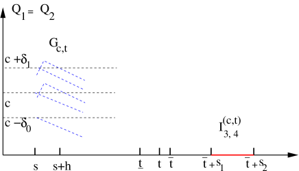
Figure 9: Sample Paths for the sets $G_{c,t}$ and $I^{(3,4)}_{c,t}$.

Note all sample paths must pass through the interval $[c-\delta_{0},c+\delta_{1}]$ at time $s$, but may continue to increase for a brief period at the beginning. After $s+h$ the two queues must be draining at rate $1-\lambda$ almost surely as shown in Lemma 8. The red interval to the right indicates periods where one of the other three queue pairs are expected to have the medium during the interval $[\overline{t}+s_{1},\overline{t}+s_{2}]$. Only one such pair will be active during this period as a result of the forthcoming construction.

The following is the earliest time that queues 1 and 2 can drain if the sample paths are constrained to lie in $G_{c,t}$,

$$\underline{t}\doteq t-\frac{\alpha_{0}}{1-\lambda}c.$$ (42)

As far as additional queue build up is concerned, under the fluid limit,

$$Q(s+h,\omega)\leq Q(s,\omega)+\lambda h=Q(s,\omega)+\lambda\nu c$$

holds for sample paths in $G_{c,t}$ (see (13)). It then follows that queues 1 and 2 will reach 0 under the fluid limit no later than

$$\overline{t}\doteq t+\frac{\alpha_{1}+\lambda\nu}{1-\lambda}c,$$ (43)

which is the definition for $\overline{t}$. We thus conclude that, under the fluid limit, queues 1 and 2 will reach 0 in the interval $(\underline{t},\overline{t})$ (for the first time after $s+h$ on occurrence of the event $G_{c,t}$). We formalize the above in the following lemma,

Lemma 12 (Queue Bounds)

Let $\tau^{0}_{c,s}\doteq\tau_{c}(s,\left\{0\right\})=\inf\left\{t\geq s:Q(t)=0\right\}$ be the first contact time with 0 for $Q=Q_{1}=Q_{2}$. Then,

$$\mu\left\{G_{c,t}\cap\left\{\omega:\tau^{0}_{c,s}(\omega)\not\in[\underline{t},\overline{t}]\right\}\right\}=0.$$

Additionally, $\forall\ell=3,4,5,6,$

$$\mu\left\{G_{c,t}\cap\left\{\omega:Q_{\ell}(\underline{t},\omega)<\Delta t\lambda_{\ell}\right\}\right\}=0,$$ (44)

where,

$$\Delta t\doteq\underline{t}-(s+h)=c(1-\alpha_{0}-\nu(1-\lambda))/(1-\lambda).$$

Proof:

By definition of $G_{c,t}$, $Q(s,\omega)\geq c-\delta_{0},\forall\omega\in G_{c,t}$. It follows that $Q$ cannot reach 0 before $\underline{t}$, as sample paths by definition lie in $P_{L}$ (see Part A.VI, following Theorem 5). A similar argument applies to $\overline{t}$.

For the last part, Lemma 3, shows that nodes $3,4,5,6$ must be idle in the period $[s+h,\underline{t}]$. Since the sample paths are restricted to lie in $P_{L}$, it follows that their queues must satisfy the stated inequality at time $\underline{t}$. The proof is complete. ∎

The time for queue $\ell$ to reach 0 following $\underline{t}$ is therefore at least,

$$f_{\ell}\doteq\Delta t\times\frac{\lambda_{\ell}}{1-\lambda_{\ell}},~{}\ell=3,4,5,6.$$

Clearly $f_{\ell}\rightarrow(c\times\lambda_{\ell})/\left((1-\lambda)\times(1-\lambda_{\ell})\right)$ as $\alpha_{0},\nu\downarrow 0$, and so this expression is bounded from below as $\alpha_{0},\alpha_{1},\nu>\chi$ are made arbitrarily small. For future use, we define

$$\underline{f}\doteq\Delta t\wedge_{\ell=3}^{6}\lambda_{\ell}/(1-\lambda_{\ell}),$$

as a lower bound on the time needed to drain any queue $\ell=3,4,5,6$.

Our results thus far do not rule out the possibility that there is an idle period during which queues 3, 4, 5, 6 fail to obtain the medium. In order to make allowance for this, we introduce a period $\xi c$, $\xi>0$, which comes following queues 1 and 2 draining, and to be definite, we set $\xi c=\underline{f}/8$. Hence, if it is the case that

$$\overline{t}-\underline{t}<\underline{f}/4$$ (45)

and that service of queue $\ell$ cannot start before $\underline{t}-\xi c$ and must have started no later than $\overline{t}+\xi c$, then it follows that service will continue throughout the interval $[\overline{t}+\xi c,\overline{t}+\xi c+\underline{f}/2]$. In this case, we may take $s_{1}=\underline{f}/4,s_{2}=\underline{f}/2$ again to be definite. Further, set $s_{3}=\xi c+\underline{f}/2$. To summarize, if (45) holds, on occurrence of $G_{c,t}$ and that service of queues 3 and 4 commences in the interval $[\underline{t}-\xi c,\overline{t}+\xi c]$, then the event $I^{(3,4)}_{c,t}$ must take place. The same is true in case service commences for either queue pair $(4,5)$ or $(5,6)$ in $[\underline{t}-\xi c,\overline{t}+\xi c]$.

Let $\hat{C}_{k},k=3,4,5,6$, be the residual time to backoff for queues 3, 4, 5, 6, at time $s+h$, with $\hat{C}_{1}=\hat{C}_{2}=0$ as these queues will be almost surely active. Define $S_{M}$ to be the number of steps in the jump chain before one of these nodes gains the medium and also define

$$W^{(3,4)} \doteq \left\{\hat{C}_{3}<\wedge_{k=4}^{6}\hat{C}_{k}\right\}\cup\left(\left\{\hat{C}_{4}<\hat{C}_{3}\wedge\hat{C}_{5}\wedge\hat{C}_{6}\right\}\cap\left\{\hat{C}_{3}<\hat{C}_{5}\right\}\right),$$ (46)

$$C^{(3,4)}_{c,t,R} \doteq W^{(3,4)}\cap\left\{S_{M}\leq\sqrt{R}\right\}.$$

$W^{(3,4)}$ is the event that queues 3 and 4 win the backoff competition to take the medium first from queues 1 and 2. Similar definitions can be made for queues $(4,5)$ and for queues $(5,6)$ in addition. The probabilities of these events are

$${\mathbb{P}}\{W^{(3,4)}\}=\frac{3}{8}={\mathbb{P}}\{W^{(5,6)}\},~{}{\mathbb{P}}\{W^{(4,5)}\}=\frac{1}{4},$$ (47)

as the backoff periods are unit mean i.i.d. exponential random variables. $C^{(3,4)}_{c,t,R}$ is the event that queues $(3,4)$ win the backoff competition and that it does so in no more than $\sqrt{R}$ of the jump chain steps when queues 1 and 2 are in backoff together.

Next let

$$B_{R}^{(1,2)}\doteq N_{R}^{(1,2)}(s+h,\underline{t}-\xi c)\cap\{W^{R}(s+h,\overline{t}+\xi c)\geq 2\sqrt{R}\}$$

be the intersection of the event $N_{R}^{(1,2)}(s+h,\underline{t}-\xi c)$ that neither queue 1 nor queue 2 starts to backoff during the time interval $[s+h,\underline{t}-\xi c]$ and the event $\{W^{R}(s+h,\overline{t}+\xi c)\geq 2\sqrt{R}\}$ that queues 1 and 2 operating in isolation would be simultaneously in backoff for a cumulative period of time of at least $2\sqrt{R}$ during the interval $[s+h,\overline{t}+\xi c]$. Informally speaking, the event $B_{R}^{(1,2)}$ ensures that there is sufficient backoff by queues 1 and 2 and that they do not begin to backoff whilst there are a significant number of queue 1 or queue 2 packets remaining.

Next define $c_{Q}$ to be,

$$c_{Q}\doteq\frac{s_{3}-s_{2}}{2}\times\left(1-\lambda_{3}\right)>0,$$

which is at least half the content of queues 3 and 4 on the fluid scale at time $\overline{t}+s_{2}$, given our construction. Further, define the following event

$$Q_{R}^{(3,4)}(\underline{t},\overline{t}+s_{2})\doteq\left\{\omega:\inf\left\{Q^{R}_{m}(u,\omega),u\in[\underline{t},\overline{t}+s_{2}]\right\}>c_{Q},m=3,4\right\}\in{\cal F}_{\overline{t}+s_{2}},$$ (48)

for which we obtain the following corollary.

Corollary 4

$$\lim_{R\rightarrow\infty}\mu_{R}\left\{G_{c,t}\cap\left(Q_{R}^{(3,4)}\right)^{c}\right\}=0$$

Proof:

Lemma 12 implies that for all $n$ sufficiently large,

$$\limsup_{R\rightarrow\infty}\mu_{R}\left\{G_{c,t}\cap\left\{\omega:Q^{R}_{\ell}(\underline{t},\omega)\leq\Delta t\lambda_{\ell}-1/n\right\}\right\}=0,~{}\ell=3,4,$$

on using Theorem 2.1 in [1] and that both the above sets are closed. Hence we need only show that,

$$\lim_{R\rightarrow\infty}\mu_{R}\left\{\left\{\omega:Q^{R}_{\ell}(\underline{t},\omega)>\Delta t\lambda_{\ell}-1/n,\ell=3,4\right\}\cap\left(Q_{R}^{(3,4)}\right)^{c}\right\}=0,$$ (49)

for sufficiently large $n$. However (49) follows from the weak law of large numbers, from the definition of $\Delta t$, $c_{Q}$, and the event $Q_{R}^{(3,4)}$. ∎

Finally, define $N_{R}^{(3,4)}(\underline{t},\overline{t}+s_{2})$ to be the event that neither queue 3 nor queue 4 has a backoff during the time interval $[\underline{t},\overline{t}+s_{2}]$ (on the fluid scale). Clearly, equivalent definitions for this and the above and the above corollary can be made for queue pairs $(4,5),(5,6)$.

In what follows it will be convenient to write $G:=G_{c,t}$. Our aim now is to show that no matter what trajectory the fluid limit path followed earlier, if it lies in $G$ so that queues 1 and 2 almost surely reach 0 in the interval $[\underline{t},\overline{t}]$, marking the end of an $M_{1}$ period, then the probability of the next period depends only on the residual backoff times, which is a Markov property.

Lemma 13

Suppose that $G$ is a set of paths as defined in (40), with parameter values so that (45) holds, and is also a $\mu$-continuity set. In addition, let $F\in{\cal F}_{s}$ be an arbitrary closed, finite-dimensional set of paths defined by times $s$ and earlier. It then holds that

$$\mu_{G}\left\{F\cap I^{(3,4)}_{c,t}\right\} \geq \frac{3}{8}\mu_{G}\left\{F^{o}\right\}$$

$$\mu_{G}\left\{F\cap I^{(5,6)}_{c,t}\right\} \geq \frac{3}{8}\mu_{G}\left\{F^{o}\right\}$$

$$\mu_{G}\left\{F\cap I^{(4,5)}_{c,t}\right\} \geq \frac{1}{4}\mu_{G}\left\{F^{o}\right\}$$

In case $F$ is a $\mu$-continuity set, the interior can be dropped and $\geq$ replaced with equality.

Proof:

We first show the last part of the lemma, assuming the first part to be true. If $F$ is a $\mu$-continuity set, then by definition, $0=\mu\left\{\partial F\right\}\geq\mu\left\{G\cap\partial F\right\}$ and it follows that $F$ is a $\mu_{G}$-continuity set as well. Since the factors sum to 1 and the events on the left are almost surely exclusive as a consequence of Lemma 3, we can now replace the inequality sign with equality.

We move to the first part of the lemma, which we will prove for queues 3 and 4. The proof for the other queue pairs is similar.

First observe that

$$C^{(3,4)}_{c,t,R}\cap B_{R}^{(1,2)}\cap N_{R}^{(3,4)}(\underline{t},\overline{t}+s_{2})\subseteq I^{(3,4)}_{c,t},$$

since $C^{(3,4)}_{c,t,R}\cap B_{R}^{(1,2)}$ implies that queues 3 and 4 activate before time $\overline{t}+s_{1}$, while $N_{R}^{(3,4)}(\underline{t},\overline{t}+s_{2})$ ensures that neither queue 3 nor queue 4 has a backoff during the time interval $[\underline{t},\overline{t}+s_{2}]$. We thus obtain the following chain of inequalities

$$\mu_{G}^{(R)}\left\{F\cap I^{(3,4)}_{c,t}\right\} \geq \mu_{G}^{(R)}\left\{F\cap C^{(3,4)}_{c,t,R}\cap B_{R}^{(1,2)}\cap N_{R}^{(3,4)}\right\}$$

$$\geq \mu_{G}^{(R)}\left\{F\cap W^{(3,4)}\right\}-\mu_{G}^{(R)}\left\{\left(\left\{S_{M}\leq\sqrt{R}\right\}\cap B_{R}^{(1,2)}\cap N_{R}^{(3,4)}\right)^{c}\right\}$$

$$\geq \frac{3}{8}\mu_{G}^{(R)}\left\{F\right\}-\mu_{G}^{(R)}\left\{S_{M}>\sqrt{R}\right\}-\mu_{G}^{(R)}\left\{\left(B_{R}^{(1,2)}\right)^{c}\right\}-\mu_{G}^{(R)}\left\{\left(N_{R}^{(3,4)}\right)^{c}\right\},$$

with $N_{R}^{(3,4)}\equiv N_{R}^{(3,4)}(\underline{t},\overline{t}+s_{2})$ for compactness. The first line follows by inclusion, the second using $\mu_{G}\left\{A\cap B\right\}\geq\mu_{G}\left\{A\right\}-\mu_{G}\left\{B^{c}\right\}$, and the third from (47) by independence of the back-off clocks and by using the union bound in conjunction with de Morgan’s laws. We now proceed to show that

$$\mu^{(R)}_{G,1} \doteq \mu_{R}\left\{S_{M}>\sqrt{R}\right\}\rightarrow 0$$

$$\mu^{(R)}_{G,2} \doteq \mu_{R}\left\{\left(B_{R}^{(1,2)}\right)^{c}\cap G_{c,t}\right\}\rightarrow 0$$

$$\mu^{(R)}_{G,3} \doteq \mu_{R}\left\{\left(N_{R}^{(3,4)}\right)^{c}\cap G_{c,t}\right\}\rightarrow 0$$

The first limit is immediate.

In order to deal with the second limit, define the event

$$Q_{R}^{(1,2)}(s+h,\underline{t}-\xi c)\doteq\left\{\omega:\inf\left\{Q^{R}_{m}(u,\omega),u\in[s+h,\underline{t}-\xi c]\right\}>\varsigma,m=1,2\right\}\in{\cal F}_{\underline{t}-\xi c}$$

for some small constant $\varsigma>0$, and use the upper bound

$$\mu^{(R)}_{G,2}\leq\mu_{R}\left\{\left(B_{R}^{(1,2)}\right)^{c}\cap Q_{R}^{(1,2)}(s+h,\underline{t}-\xi c)\cap G_{c,t}\right\}+\mu_{R}\left\{\left(Q_{R}^{(1,2)}(s+h,\underline{t}-\xi c)\right)^{c}\cap G_{c,t}\right\}$$

The limit of the second term is 0 by definition of $\underline{t}$ as the earliest time that queues 1 and 2 can drain under the event $G_{c,t}$ and on making a suitable choice for $\varsigma$. It suffices then to show that the limit of the first term is 0. In order to prove this, we invoke the definition of the event $B_{R}^{(1,2)}$ to obtain that the first term is bounded from above by

$$\mu_{R}\left\{\left(N_{R}^{(1,2)}(s+h,\underline{t}-\xi c)\right)^{c}\cap Q_{R}^{(1,2)}(s+h,\underline{t}-\xi c)\right\}+\mu_{R}\left\{\{W^{R}(s+h,\overline{t}+\xi c)\leq 2\sqrt{R}\}\cap G_{c,t}\right\}$$

That the first term converges to 0 follows by definition of the events and Lemma 7. Lemma 11 shows that the limit of the second term (i.e. the event there is insufficient backoff by queues 1 and 2 on occurrence of $G_{c,t}$) is 0.

In order to handle the third limit, we apply the upper bound

$$\mu^{(R)}_{G,3}\leq\mu_{R}\left\{\left(N_{R}^{(3,4)}(\underline{t},\overline{t}+s_{2})\right)^{c}\cap Q_{R}^{(3,4)}\right\}+\mu_{R}\left\{\left(Q_{R}^{(3,4)}\right)^{c}\cap G_{c,t}\right\}$$

Lemma 7 shows that the limit of the first term is 0, whilst the statement of Corollary 4 is that the limit of the second term is 0.

Taking limits in (C) with respect to $R$, and using Lemma 10, it follows that,

$$\mu_{G}\left\{F\cap I^{(3,4)}_{c,t}\right\} \geq \frac{3}{8}\limsup_{R}\mu_{G}^{(R)}\left\{F\right\}$$

$$\geq \frac{3}{8}\liminf\mu_{G}^{(R)}\left\{F^{o}\right\}$$

$$\geq \frac{3}{8}\mu_{G}\left\{F^{o}\right\}$$

where the first inequality follows from the fact that $F$ and $I^{(3,4)}_{c,t}$ are both closed and the third since $F^{o}$ is open and again from Lemma 10. ∎

Let $\mu$ be the fluid limit measure and proceed to define for any given $t\geq 0$ the following class of sets, the finite-dimensional continuity rectangles ${\cal K}_{\mu,t}$ which are a subset of the finite-dimensional sets, ${\cal H}_{t}$.

Definition 7

Define the class of finite closed rectangles ${\cal R}$ to be the sets,

$$\left(\prod_{j=1}^{N}[q_{j,L},q_{j,H}]\right)\times\left(\prod_{j=1}^{N}[r_{j,L},r_{j,H}]\right)\subset{\mathbb{R}}_{+}^{N}\times{\mathbb{R}}_{+}^{N},$$

where $q_{j,L}\leq q_{j,H},r_{j,L}\leq r_{j,H}$, otherwise we obtain the empty set.

Given times $0\leq t_{1}<t_{2}<\cdots<t_{J}\leq t$, define $\pi_{J,t}:C[0,\infty)\rightarrow E^{J}$ to be the (continuous) projection map taking the sample path to its position at times $t_{1},\cdots,t_{J}$

$$\pi_{K,t}(\omega)=\Big{(}\left({\bf Q}(t_{1},\omega),{\bf I}(t_{1},\omega)\right),\cdots,\left({\bf Q}(t_{J},\omega),{\bf I}(t_{J},\omega)\right)\Big{)}.$$

Finally, take ${\cal R}^{J}$ to be $J$-products of closed rectangles. Define ${\cal K}_{t}$ to be sets of the form $\pi_{K,t}^{-1}R_{J},R_{J}\in{\cal R}^{J}$ and finally ${\cal K}_{\mu,t}\subset{\cal K}_{t}$ to be those $H\in{\cal K}_{t}$ such that $\mu\left\{\partial H\right\}=0$. Clearly ${\cal K}_{\mu,t}\subset{\cal K}_{t}\subset{\cal F}_{t}$.

Returning to Lemma 13, we see that it is satisfied by all sets $F\in{\cal K}_{\mu,s}$ with equality since they are by definition closed $\mu$-continuity sets. Furthermore, since the terms on the left and on the right are measures and since ${\cal K}_{\mu,s}$ generates ${\cal F}_{s}$, the following corollary holds.

Corollary 5

$\forall F\in{\cal F}_{s}$, Lemma 13 holds with equality, i.e.

$$\mu_{G}\left\{F\cap I^{(3,4)}_{c,t}\right\} = \frac{3}{8}\mu_{G}\left\{F\right\}$$

$$\mu_{G}\left\{F\cap I^{(5,6)}_{c,t}\right\} = \frac{3}{8}\mu_{G}\left\{F\right\}$$

$$\mu_{G}\left\{F\cap I^{(4,5)}_{c,t}\right\} = \frac{1}{4}\mu_{G}\left\{F\right\}$$

Proof:

First note that the measures on the LHS and RHS are both finite and are therefore both $\sigma$-finite, with respect to the sets in ${\cal K}_{\mu,s}$. It is readily shown that ${\cal K}_{\mu,s}$ is a $\pi$-system and $\sigma({\cal K}_{\mu,s})={\cal F}_{s}$. Theorem 10.3 in [2] thus shows that LHS and RHS agree on ${\cal F}_{s}$. ∎

To continue towards Theorem 7, we now define paths that one of which is followed immediately on completion of a (positive) $M_{1}$-period at time $s$, $\mu$ a.s. First define

$$\vartheta_{s,t}^{({\bf Q},M_{k})}(u),~{}u\in[s,t],k=2,3,4,$$ (52)

to be the path which is at ${\bf Q}$ at time $s$ and then follows $M_{k}$ until time $t$, e.g., if $k=1$, queues 1 and 2 are decreasing linearly at rate $(1-\lambda)$ and any other queue $\ell=3,4,5,6$ is increasing at rate $\lambda_{\ell}$. Precise definitions we omit as the form of the sample paths have already been discussed. The next definition is for an indicator function that the above path is being followed in an interval $[s,s+h],h>0$.

$${\rm 1\rule{0.43057pt}{6.54443pt}^{(s,h,\eta)}_{M_{k},{\bf Q}}}\doteq{\rm 1\rule{0.43057pt}{6.54443pt}\hskip 0.86108pt}\left\{\omega:\lvert\lvert{\bf Q}(v,\omega)-\vartheta_{s,s+h}^{({\bf Q}(s,\omega),M_{k})}(v)\rvert\rvert<\eta,v\in[s,s+h]\right\}.$$ (53)

In words $M_{k}$ is ”followed” for an interval of duration $h$ starting at $s$ to a closeness $\eta$.

Note that the result of Corollary 5 applies only to events in some $\sigma$-algebra ${\cal F}_{w}$ where $w\geq 0$ is fixed. However, we require that equivalent results be established for all events $F\in{\cal F}_{Z^{(1,2)}_{m,n}}$. This issue can be approached as follows.

Given $s<t,a<b$, with $n\in{\mathbb{N}}_{0}$ and recalling Definition 4, set

$$C^{(n)}\doteq\left\{\omega:(Z^{(1,2)}_{m,n},A^{(1,2)}_{m,n})\in[s,t)\times[a,b)\right\},~{}~{}$$

then it is readily seen that,

$$F\cap C^{(n)}\in{\cal F}_{t},~{}\forall F\in{\cal F}_{Z^{(1,2)}_{m,n}}^{.}$$

Suppose that $s<t$ in the definition of $C^{(n)}$ satisfy $t-s<\lambda_{1}e_{m},$ and $e_{m}<a<b\leq f_{m}$ ($e_{m}$ and $f_{m}$ are given in Definition 4). Then, it can be seen that for all paths $\omega\in F\cap C^{(n)}$, for any $F\in{\cal F}_{Z^{(1,2)}_{m,n}}$, we can find a $w<s$ such that $I_{\ell}(s,\omega)-I_{\ell}(w,\omega)=\beta(s-w)$, $\ell=1,2$, i.e., the queues and activity components constitute a set of parallel lines over the interval $[w,s]$.

The above intuitive argument can be formalized by establishing the existence of an equivalent $\sigma$-algebra. We say that the $\sigma$-algebra ${\cal F}_{Z^{(1,2)}_{m,n}}\cap C^{(n)}$ is equivalent to a sub $\sigma$-algebra, ${\cal H}_{w}\subset{\cal F}_{w}$, if to each event $H\in{\cal F}_{Z^{(1,2)}_{m,n}}\cap C^{(n)}$ there is an event $H_{w}\in{\cal H}_{w}$ so that $H=H_{w}$.

Lemma 14 (Equivalent $\sigma$-algebra)

Given $n\in{\mathbb{N}}_{0}$, arbitrary $t>s\geq 0$ such that $t-s<\lambda_{1}e_{m}$, and $e_{m}<a<b\leq f_{m}$ and arbitrary $w\in(t-\lambda_{1}e_{m},s)$, there is a $\sigma$-algebra, ${\cal H}_{w}\subset{\cal F}_{w}$ equivalent to ${\cal F}_{Z^{(1,2)}_{m,n}}\cap C^{(n)}$.

We omit the proof. Set $t_{Z}=Z^{(1,2)}_{m,n}$, $h^{(1,2)}=\lambda_{1}e_{m}\times\wedge_{\ell=3}^{6}\lambda_{\ell}/(1-\lambda_{\ell}),$ and ${\bf Q}_{Z}={\bf Q}(Z^{(1,2)}_{m,n})$. Next define ${\rm 1\rule{0.43057pt}{6.54443pt}^{(\eta,M_{1})}_{M_{k},m,n}}$ to be ${\rm 1\rule{0.43057pt}{6.54443pt}^{(t_{Z},h^{(1,2)},\eta)}_{M_{k},{\bf Q}_{Z}}},k=2,3,4$ if $Z^{(1,2)}_{m,n}<\infty$. Define ${\cal F}^{\infty}_{Z^{(1,2)}_{m,n}}\doteq{\cal F}_{Z^{(1,2)}_{m,n}}\cap\left\{Z^{(1,2)}_{m,n}<\infty\right\}$ as we are only interested in finite stopping times.

Theorem 7

$\forall n\in{\mathbb{N}}_{0},m\in{\mathbb{Z}}_{0}$, $\exists\eta_{m}$ such that $\forall\eta,~{}\eta_{m}>\eta>0$,

$$\mu\left\{{\rm 1\rule{0.43057pt}{6.54443pt}^{(M_{1},\eta)}_{M_{2},m,n}}|{\cal F}^{\infty}_{Z^{(1,2)}_{m,n}}\right\} = \frac{3}{8},~{}\mu~{}a.s.,$$ (54)

$$\mu\left\{{\rm 1\rule{0.43057pt}{6.54443pt}^{(M_{1},\eta)}_{M_{3},m,n}}|{\cal F}^{\infty}_{Z^{(1,2)}_{m,n}}\right\} = \frac{3}{8},$$

$$\mu\left\{{\rm 1\rule{0.43057pt}{6.54443pt}^{(M_{1},\eta)}_{M_{4},m,n}}|{\cal F}^{\infty}_{Z^{(1,2)}_{m,n}}\right\} = \frac{1}{4}.$$ (55)

Since $\eta>0$ can be taken arbitrarily small, the conclusion is that one of the periods $M_{2},M_{3},M_{4}$ start immediately at $Z^{(1,2)}_{m,n}$ on occurrence of $Z^{(1,2)}_{m,n}<\infty$ and with probabilities determined solely by the residual backoff times.

Proof:

Given $F\in{\cal F}_{Z^{(1,2)}_{m,n}}^{\infty}$, we may write $F=\cup_{k}F_{k}$ as a countable union of disjoint sets. $F_{k}$ is obtained by intersection of $F$ with the disjoint sets,

$$C_{k}\doteq\left\{\omega:(Z^{(1,2)}_{m,n},A^{(1,2)}_{m,n})\in(s_{k},t_{k}]\times(a_{k},b_{k}]\right\},$$

where $e_{m}\leq a_{k}<b_{k}\leq f_{m}$ and $e_{m}\leq s_{k}<t_{k}$ are chosen according to $\eta$ in a way to be described subsequently. $C_{k}\cap C_{m}=\emptyset,~{}m\neq k$ is constructed by first choosing the intervals for the stopping time $Z^{(1,2)}_{m,n}$ to be disjoint and then likewise the durations into disjoint semi-open intervals. Thus, $F_{k}\doteq F\cap C_{k}\in{\cal F}_{t_{k}}.$

We turn to $F_{k}$ and will suppose that $t_{k}-s_{k}$ is sufficiently small so that we may find a time $w_{k}\in(t_{k}-e_{m}\lambda_{1},s_{k})$ as in Lemma 14. $w_{k}$ will be a constant determined by $a_{k},b_{k},s_{k},t_{k}$ and $\eta$ only. For the moment suppose that $w_{k}$ and $\eta$ are used to determine constants $c_{\eta},t_{w_{k}}$ and then a set $G_{c_{\eta},t_{w_{k}}}$, satisfying the conditions of Lemma 13, such that in addition,

$$C_{k}\subset G_{c_{\eta},t_{w_{k}}},$$ (56)

with the $s$ in the definition of $G_{c,t}$, see (40), taken to be $w_{k}$. It can then be seen that the following chain of equalities hold,

$$\mu\left\{F_{k}\cap I^{(3,4)}_{c_{\eta},t_{w_{k}}}\right\} = \mu_{G_{c_{\eta},t_{w_{k}}}}\Big{\{}F_{k}\cap I^{(3,4)}_{c_{\eta},t_{w_{k}}}\Big{\}}$$

$$= \mu_{G_{c_{\eta},t_{w_{k}}}}\Big{\{}F^{(w_{k})}_{k}\cap I^{(3,4)}_{c_{\eta},t_{w_{k}}}\Big{\}}$$

$$= \frac{3}{8}\mu_{G_{c_{\eta},t_{w_{k}}}}\Big{\{}F^{(w_{k})}_{k}\Big{\}}$$

$$= \frac{3}{8}\mu_{G_{c_{\eta},t_{w_{k}}}}\Big{\{}F_{k}\Big{\}}$$

$$= \frac{3}{8}\mu\left\{F_{k}\right\}$$

The first equality follows from (56), the second from Lemma 14 as there exits a $F^{(w_{k})}_{k}\in{\cal F}_{w_{k}}$ such that $F^{(w_{k})}_{k}=F_{k}$, the third from Corollary 5 and by definition of $G_{c_{\eta},t_{w_{k}}}$, the fourth equality is again from Lemma 14, and the final one follows again from (56). Corresponding results follow for $I^{(4,5)}_{c_{\eta},t_{w_{k}}}$ and $I^{(5,6)}_{c_{\eta},t_{w_{k}}}$. Once one of these events has occurred, $\mu$ almost surely the queues corresponding to the active period proceed to empty because they lie in $P_{L}$ and therefore $P$. Moreover, $\eta_{m}$ is determined depending on the duration (at least $\lambda_{1}e_{m}$) of the $M_{1}$ period. $\eta_{m}$ is taken sufficiently small, so that if we take any $\eta,\eta_{m}>\eta>0$, only the node pair (and corresponding $M_{k}$ period) can satisfy the constraints in (53), for the interval $[Z^{(1,2)}_{m,n},Z^{(1,2)}_{m,n}+h^{(1,2)}]$.

The above steps may be taken provided that i) $G_{c_{\eta},t_{w_{k}}}$ is a closed $\mu$-continuity set, ii) $G_{c_{\eta},t_{w_{k}}}$ contains $C_{k}$ and hence $F_{k}$ iii) $\overline{t}+s_{3}-w_{k}$ is sufficiently small, so that the paths $\vartheta_{.,.}^{({\bf Q},M_{k})}$ satisfy the constraints as in (54), and iv) the condition (45) must hold so that the conditions of Lemma 13 and also of Corollary 5 are met.

To show that $c_{\eta},t_{w_{k}}$ and a corresponding $G_{c_{\eta},t_{w_{k}}}$ exist, given $\eta>0$, set $t_{k}-s_{k}=A_{1}\eta$ and $c_{\eta}=A_{2}\eta$, where $A_{1}$ and $A_{2}$ will be fixed later. Next fix the time $t_{w_{k}}=(s_{k}+t_{k})/2$. $w_{k}$ is now determined using $t_{w_{k}}-w_{k}=(1-\lambda)c_{\eta}$. A brief calculation shows that $\alpha_{0},\alpha_{1}$ must be chosen so that

$$\alpha_{0},\alpha_{1}>\frac{A_{1}(1-\lambda)}{2A_{2}},$$ (58)

in order that condition ii) above is met.

As far as i) is concerned, $G_{c,t}$ is an intersection of two sets, a queue constraint and an activity constraint, so that it is enough to obtain each as a $\mu$-continuity set. With respect to the queue constraint set, at time $w_{k}$, there are uncountably many choices for $\alpha_{0},\alpha_{1}$ which may be taken as close as we like to the constraint in (58) given $c_{\eta}$. For the activity set, we may choose $\nu$ arbitrarily small and having fixed it, then there are uncountably many choices for $\chi>0$ which we may also take arbitrarily small. Thus the activity set can also be chosen to be a $\mu$-continuity set. Putting the above together, $G$ may be constructed as a $\mu$-continuity set for given $A_{1},A_{2},\eta$ and so that $C_{k}\subset G$.

We turn to condition iv), where it can be checked that it is satisfied provided that

$$\frac{\alpha_{0}+\alpha_{1}+\lambda\nu}{1-\lambda}<\frac{1}{4}\left(\frac{1-\alpha_{0}-\nu(1-\lambda)}{1-\lambda}\wedge_{\ell=3}^{6}\frac{\lambda_{\ell}}{1-\lambda_{\ell}}\right),$$ (59)

which obviously holds by making $\alpha_{0}$, $\alpha_{1}$, and $\nu$ sufficiently small, and then choosing $A_{1}/A_{2}$ sufficiently small according to (58).

As far as iii) is concerned, an examination of the construction preceding Lemma 13 shows that $\overline{t}+s_{3}-w_{k}\propto c_{\eta}=A_{2}\eta$. We may thus proceed by taking $A_{2}>0$ sufficiently small to ensure that iii) is met and then choose $A_{1}>0$ sufficiently small so as to meet (58), (59). This fixes $c_{\eta},\nu$. The rest follows on choice of $\alpha_{0},\alpha_{1},\chi$.

Note that common choices may be made for $A_{1},A_{2},\nu$ for each $C_{k}$ and once these are fixed, common values may be chosen for $\alpha_{0},\alpha_{1},\chi$ as there are uncountably many possibilities and only a countable number of choices can have positive probability for any $C_{k}$. We have thus shown that a suitable $G_{c,t}$ can be found for each $k$, given $\eta>0$.

The rest of the proof follows on summing (C) over $k$, to obtain

$$\sum_{k}\mu\left\{{\rm 1\rule{0.43057pt}{6.54443pt}^{(t_{Z},h_{Z},\eta)}_{M_{2},{\bf Q}_{Z}}};F_{k}\right\} = \frac{3}{8}\sum_{k}\mu\left\{F_{k}\right\}$$ (60)

$$\mu\left\{{\rm 1\rule{0.43057pt}{6.54443pt}^{(t_{Z},h_{Z},\eta)}_{M_{2},{\bf Q}_{Z}}};F\right\} = \frac{3}{8}\mu\left\{F\right\},$$

and similarly for $M_{3}$ and $M_{4}$. This is the required result as $F$ is arbitrary. ∎

C.II. Switchover from $M_{2},M_{3},M_{4}$

Here we will only state our results, moreover $M_{2}$- and $M_{3}$-periods are analogous and so we will only deal with the former. To state our theorem for switching out of a $M_{2}$-period, define ${\rm 1\rule{0.43057pt}{6.54443pt}^{(M_{2},\eta)}_{M_{k},m,n}},k=1,3$ as was done for switching out of $M_{1}$. Also define ${\cal F}_{Z^{3}_{m,n}}^{\infty}\doteq{\cal F}_{Z^{3}_{m,n}}\cap\left\{Z^{3}_{m,n}<\infty\right\}$.

Theorem 8

$\forall n\in{\mathbb{N}}_{0},m\in{\mathbb{Z}}-\left\{0\right\}$, $\exists\overline{p},\overline{q}>0,\overline{p}+\overline{q}=1$ and $\exists\eta_{m}$ such that $\forall\eta,~{}\eta_{m}>\eta>0$

$$\mu\left\{{\rm 1\rule{0.43057pt}{6.54443pt}^{(M_{2},\eta)}_{M_{1},m,n}}|{\cal F}_{Z^{3}_{m,n}}^{\infty}\right\} = \overline{p},~{}\mu~{}a.s.,$$ (61)

$$\mu\left\{{\rm 1\rule{0.43057pt}{6.54443pt}^{(M_{2},\eta)}_{M_{3},m,n}}|{\cal F}_{Z^{3}_{m,n}}^{\infty}\right\} = \overline{q}.$$

The quantities $\overline{p},\overline{q}$ are determined as follows,

$$\overline{p} = \sum_{X=0}^{\infty}\sum_{X_{4}=0}^{\infty}\sum_{U_{4}=0,1}b^{(3)}(X)\pi^{\infty}_{4}(X_{4},U_{4})c_{1}^{X}(X_{4},U_{4})$$ (62)

$$\overline{q} = \sum_{X=0}^{\infty}\sum_{X_{4}=0}^{\infty}\sum_{U_{4}=0,1}b^{(3)}(X)\pi^{\infty}_{4}(X_{4},U_{4})c_{5}^{X}(X_{4},U_{4})$$

where $\pi^{\infty}_{4}(X_{4},U_{4})$ is the equilibrium jump chain probability that node 4 is in state $(X_{4},U_{4})$ when operating in isolation (i.e., when node 4 is the only node in the network). $b^{(3)}(X)$ is the limiting probability as $X^{3}_{0}\uparrow\infty$ that a first backoff of node 3 occurs when $X_{3}=X$, service starting with $X^{3}_{0}$ packets. $c_{1}^{X}(X_{4},U_{4})$ is the probability that node 1 or 2 first gain the medium when node 3 has a first backoff with $X_{3}=X$ packets and the state of node 4 as given. The remaining definitions for $\overline{q}$ are similar. Thus in this case there is no simple formula and $\overline{p},\overline{q}$ depend on the backoff parameter $\gamma$ as well as the arrival rates to nodes 3 and 4.

For the case of switching out of $M_{4}$ we have the following result, again making the corresponding definitions as in Theorem 7.

Theorem 9

For any $Z^{(4,M_{4}^{(5)})}_{m,n}$ stopping time, there is a $\eta_{m}>0$ sufficiently small so that, for all $\eta_{m}>\eta>0$

$$\mu\left\{{\rm 1\rule{0.43057pt}{6.54443pt}^{(M_{2},\eta)}_{M_{4},m,n}}\vee{\rm 1\rule{0.43057pt}{6.54443pt}^{(M_{3},\eta}_{M_{4},m,n)}}~{}~{}|~{}{\cal F}_{Z^{(4,M_{4}^{(5)})}_{m,n}}^{\infty}\right\}=1\,~{}\mu~{}a.s.,$$ (63)

and so that

$$\mu\left\{{\rm 1\rule{0.43057pt}{6.54443pt}^{(M_{1},\eta)}_{M_{4},m,n}}|{\cal F}_{Z^{(4,M_{4}^{(5)})}_{m,n}}^{\infty}\right\} = 0,~{}\mu~{}a.s..$$ (64)

A similar result holds for $Z^{(5,M_{4}^{(4)})}_{m,n}$ stopping times.

This concludes Part C.

Appendix D Fluid limit proofs: Part D

In parts A-C we have established a) saw tooth properties and some constraints on those sample paths, b) what will occur at the end of a given $M_{k}$-period, $k=1,2,3,4$ and c) that a natural state will be entered in finite time before the network can empty almost surely. What has not been shown, is whether any $M_{1}$-period would ensue at all. The purpose of this section is to show that $M_{1}$-periods will occur $\mu$ a.s. following a natural state, provided $\rho$ is sufficiently close to 1.

In fact, establishing this result is not strictly needed to prove instability. If there is a last visit to queues 1 and 2 (which might occur when they are both empty), then these two queues must grow linearly and therefore the fluid system is unstable. Nevertheless, we will show that an infinite sequence of $M_{1}$-periods will occur $\mu$ almost surely and in strictly bounded time, following $T_{N}$ to enter a non-empty natural state,

Denote by $\tau^{(1,2)}_{p}:C[0,\infty]\rightarrow[0,\infty]$ as the first point of increase of either $I_{1},I_{2}$, as in Definition 5, following $T_{N}$. It is easily shown that $\tau^{(1,2)}_{p}$ is a ${\cal F}_{t^{+}}$ stopping time, and corresponds to the start of a positive $M_{1}$-period. Our main result is:

Theorem 10

There exists a $0<T_{V}<\infty$ such that $\tau^{(1,2)}_{p}<T_{N}+T_{V},$ $\mu~{}a.s$.

We first show that the issue of occurrence of an $M_{1}$-period arises only when there is at least one zero queue. To see this, consider the network at time $T_{N}$, and, without loss of generality, suppose $T_{N}>0$. If $Q_{\ell}(T_{N})=q_{\ell}>0,~{}\ell=1,\cdots,6$ then continuity implies that this actually holds for some small interval $[T_{N}-\xi,T_{N}]$, depending on $\omega$, with $\xi>0$. During any such interval, one of the periods $M_{1},\cdots,M_{4}$ has to be active, with probability 1, as a consequence of Lemma 9. Moreover if the active period is not $M_{1}$, then one will follow in bounded time $\tau^{(1,2)}_{p}<T_{N}+T_{S}$, as a consequence of Theorems 7, 8 and 9 and because the subnetwork determined by nodes 3, 4, 5 ,6 is work conserving once a natural state is entered. Next, consider the cases where a subset of queues $\{q_{1},q_{2},q_{3},q_{6}\}$ are 0. Rather than deal with all every such cases, we will consider just one. The approach for the remaining cases will then become apparent. We therefore focus on the case $q_{3}=q_{4}=q_{5}=q_{6}=0$ with $q_{1}\vee q_{2}>0$ and show that $\tau^{(1,2)}_{p}$ is effectively $T_{N}$ on the fluid scale. Other cases are simpler to address.

For the above case, it will be sufficient to prove the following lemma,

Lemma 15

Given $\epsilon>0,\eta>0$, and $Q^{(\ell)}_{L}<Q^{(\ell)}_{H},\ell=1,2$ with $Q^{(1)}_{L}\vee Q^{(2)}_{L}>0$ there exists $\delta>0$, such that,

$$\liminf_{R\rightarrow\infty}\mu_{R}\left\{\tau^{(1,2)}_{p}>T_{N}+\epsilon;Q_{\ell}^{R}(T_{N})<\delta,\ell=3,4,5,6,Q^{R}_{\ell}(T_{N})\in(Q^{(\ell)}_{L},Q^{(\ell)}_{H}),\ell=1,2\right\}<\eta.$$

It then follows that $\mu\left\{\tau^{(1,2)}_{p}>T_{N}+\epsilon;~{}Q_{\ell}(T_{N})=0,\ell=3,4,5,6;Q_{\ell}\in(Q^{(\ell)}_{L},Q^{(\ell)}_{H}),\ell=1,2\right\}=0$ by Theorem 2.1 of [1]. This implies our result since $\epsilon>0$ was arbitrary.

The proof of Lemma 15 is strongly specific to our choice of network and so we only provide a sketch of the proof, which relies on the following definition. Consider the sequence of queue activations in the network and in particular node 4 and 5 activations.

Definition 8

A control step, at index $k$ of the jump chain, is $C_{J,k}\in\left\{4,5\right\}$. At index 0, it is 4, unless only node 5 is active, in which case it is 5. At any subsequent index $k\geq 1$, the control step is determined as follows: (i) if both nodes 4 and 5 are active at index $k$, $C_{J,k}$ is the node that has become active first, (ii) If only one is active, $C_{J,k}$ is the active node, (iii) if neither, then $C_{J,k}$ is the last node that was active.

A control swap to control step 5 occurs at step $k$ if $C_{J,k-1}=4$ and $C_{J,k}=5$, and vice versa for a control swap to control step 4. These events are denoted as $4\rightarrow 5$ and $5\rightarrow 4$. The step at which the $r$-th control swap takes place is a (discrete) stopping time $\tau^{(S)}_{r}$.

For the subnetwork of nodes 3, 4, 5, 6 in isolation, it is readily shown that the probability is 1 that an infinite number of control swaps occur, $\tau^{(S)}_{r}<\infty$, $\tau^{(S)}_{1}<\tau^{(S)}_{2}<\ldots$, with corresponding filtration $\left\{{\cal G}_{r}\right\}_{r\in{\mathbb{N}}}$.

Next let $S$ be the stopping time until one of nodes 1 and 2 gain the medium (this event is blocked since we are considering the subnetwork in isolation). Using the properties of our network it can then be shown that,

Lemma 16

$\exists\epsilon>0$ and $N_{S}\in{\mathbb{N}}$ such that $\forall r\in{\mathbb{N}}$, ${\mathbb{P}}\{S<r+N_{S}~{}|~{}{\cal G}_{r}\}>\epsilon$.

The proof relies on showing that once a control swap has taken place say $4\rightarrow 5$ then within a bounded number of additional control swaps either it will occur that node 3 has a backoff with $Q_{4}=0$ or node 6 has a backoff with $Q_{5}$ = 0 and with probability at least $\epsilon>0$.

The result of Lemma 16 implies that $m_{S}={\mathbb{E}}\left[{\displaystyle S}\right]<\infty$ and actually that ${\mathbb{P}}\{S>rN_{S}\}<\left(1-\epsilon\right)^{r}$, see [42] for example. That is nodes 1 and 2 will gain the medium within a number of control swaps which has finite expectation. It then follows from Markov’s inequality, that given any $\eta>0$, there is a number of control swaps $M_{\eta}$ such that ${\mathbb{P}}\{S>M_{\eta}\}<\eta$.

Given the above, in proving Lemma 15 it will be enough to show the following lemma.

Lemma 17

Suppose that given any $\delta_{1}>0$, the sequence of initial conditions (starting from 0) for the jump chain of the subnetwork, determined by nodes $3,4,5,6$, satisfies $Q_{\ell}(0)<\delta_{1}R$, for $R$ sufficiently large.

Furthermore, given $\epsilon>0,\eta>0$ and any fixed number of control swaps $M_{\eta}\in{\mathbb{N}}$, let $X_{M_{\eta}}$ be the total number of steps to complete $M_{\eta}$ control swaps. Then $\exists\delta>0$ such that for all $R$ sufficiently large

$${\mathbb{P}}\{X_{M_{\eta}}>\lceil R\epsilon\rceil|~{}Q_{\ell}(0)\leq\delta R,\ell=3,\cdots,6\}<\eta.\\$$

The result of the lemma clearly relies on the supposed initial conditions. It can be demonstrated via a construction. The construction works by determining $M_{\eta}$ intervals so that the probability of a control swap in each is close to 1 and so the total queue length at the start of each interval is small based on the arrivals which might have taken place during previous intervals. The proof is then completed by showing that given any control step at the start of an interval, say 5, a swap $5\rightarrow 4$ will occur with high probability in a number of steps in proportion to the initial condition for the interval. Since only $M_{\eta}$ such intervals are required, a $\delta$ can be obtained accordingly.

Other cases are dealt with similarly but there is some positive but bounded delay before an $M_{1}$-period occurs. For example if $q_{1}=q_{2}=q_{6}=q_{5}=0$ and $q_{3}>0$, then one shows that a $M_{2}$-period occurs in negligible fluid time.

Thus in all the cases, we may can show that $M_{1}$-periods occur within bounded fluid time following a natural state. This concludes Part D.

Appendix E Additional proofs

E.I. Proof of Lemma 1

The proof relies on basic sample path properties of the fluid limit process $\{Q(t)\}$ as described in Subsection IV-A. First of all, the $M_{1}$-period that initiates the $i$-th cycle ends at time $t_{i}+T_{i1}$, with

$$T_{i1}=\max\left\{\frac{Q_{1}(t_{i})}{1-\rho_{1}},\frac{Q_{2}(t_{i})}{1-\rho_{2}}\right\}\leq\frac{\max\{Q_{1}(t_{i}),Q_{2}(t_{i})\}}{1-\rho_{0}}\leq\frac{L(t_{i})}{1-\rho_{0}}.$$

Define $K(t)=\max\{Q_{3}(t),Q_{4}(t)\}+\max\{Q_{5}(t),Q_{6}(t)\}$ and recall that $\rho=\rho_{0}+\rho_{3}+\rho_{6}$. Then

$$K(t_{i}+T_{i1}) \leq K(t_{i})+(\rho_{3}+\rho_{6})T_{i1}$$

$$\leq L(t_{i})-\max\{Q_{1}(t_{i}),Q_{2}(t_{i})\}+(\rho_{3}+\rho_{6})\frac{\max\{Q_{1}(t_{i}),Q_{2}(t_{i})\}}{1-\rho_{0}}$$

$$= L(t_{i})-\frac{(1-\rho)\max\{Q_{1}(t_{i}),Q_{2}(t_{i})\}}{1-\rho_{0}}$$

$$= L(t_{i})-(1-\rho)T_{i1},$$

which may also be seen from the fact that $L(t)$ decreases at a rate $1-\rho$ or larger during the time interval $[t_{i},t_{i}+T_{i1}]$ and $K(t_{i}+T_{i1})=L(t_{i}+T_{i1})$ since $Q_{1}(t_{i}+T_{i1})=Q_{2}(t_{i}+T_{i1})=0$.

Define $T_{0}=\frac{K(t_{i}+T_{i1})}{1-\rho_{3}-\rho_{6}}$. We distinguish between two cases, depending on whether an $M_{4}$-period starts before time $t_{i}+T_{i1}+T_{0}$ or not.

If no $M_{4}$-period occurs before time $t_{i}+T_{i1}+T_{0}$, then $K(t)$ decreases at a rate $1-\rho_{3}-\rho_{6}$ or larger for all $t\in[t_{i}+T_{i1},t_{i}+T_{i1}+T_{0}]$ and reaches zero no later than time $t_{i}+T_{i1}+T_{0}$, unless an $M_{1}$-period intervenes. This implies that the next $M_{1}$-period must start no later than time $t_{i}+T_{i1}+T_{0}$.

Using the above results, a simple calculation shows that

$$\Delta t_{i}\leq T_{i1}+T_{0}\leq T_{i1}+\frac{L(t_{i})-(1-\rho)T_{i1}}{1-\rho_{3}-\rho_{6}}\leq\frac{L(t_{i})}{(1-\rho_{0})(1-\rho_{3}-\rho_{6})}\leq C_{T}L(t_{i}).$$

Also, $L(t)$ has continuously decreased during the cycle, so $L(t_{i+1})-L(t_{i})\leq 0$.

Now suppose that an $M_{4}$-period does start at some time $t_{0}\in[t_{i}+T_{i1},t_{i}+T_{i1}+T_{0}]$, and ends at time $u_{0}$.

Since $K(t)$ decreases at a rate $1-\rho_{3}-\rho_{6}$ or larger during the time interval $[t_{i}+T_{i1},t_{0}]$, it follows that

$$K(t_{0})\leq K(t_{i}+T_{i1})-(1-\rho_{3}-\rho_{6})(t_{0}-t_{i}-T_{i1}).$$

Noting that $Q_{4}(t_{0}),Q_{5}(t_{0})\leq K(t_{0})$, we conclude that the duration of the $M_{4}$-period is no longer than

$$u_{0}-t_{0}\leq\min\left\{\frac{Q_{4}(t_{0})}{1-\rho_{4}},\frac{Q_{5}(t_{0})}{1-\rho_{5}}\right\}\leq\frac{K(t_{0})}{1-\max\{\rho_{4},\rho_{5}\}}.$$

Since $K(t)$ increases at a rate no larger than $\rho_{3}+\rho_{6}$ during the time interval $[t_{0},u_{0}]$, it follows that

$$K(u_{0})\leq K(t_{0})+(\rho_{3}+\rho_{6})(u_{0}-t_{0}).$$

The $M_{4}$-period will cause the queue of node 4 to empty at some point and become smaller than the queue of node 3, and likewise the queue of node 5 must empty at some point and become smaller than the queue of node 6. Because $M_{4}$-periods can no longer be initiated from $M_{2}$ and $M_{3}$, $K(t)$ decreases at a rate $1-\rho_{3}-\rho_{6}$ or larger from time $u_{0}$ onward, and reaches zero no later than time $u_{0}+\frac{K(u_{0})}{1-\rho_{3}-\rho_{6}}$, unless an $M_{1}$-period intervenes. This implies that the next $M_{1}$-period must start no later than time $u_{0}+\frac{K(u_{0})}{1-\rho_{3}-\rho_{6}}$.

Combining the above results, we obtain

$$\Delta t_{i} \leq u_{0}+\frac{K(u_{0})}{1-\rho_{3}-\rho_{6}}-t_{i}=T_{i1}+(t_{0}-t_{i}-T_{i1})+(u_{0}-t_{0})+\frac{K(u_{0})}{1-\rho_{3}-\rho_{6}}$$

$$\leq T_{i1}+(t_{0}-t_{i}-T_{i1})+\frac{K(t_{0})+(u_{0}-t_{0})}{1-\rho_{3}-\rho_{6}}$$

$$\leq T_{i1}+(t_{0}-t_{i}-T_{i1})+\left(1+\frac{1}{1-\max\{\rho_{4},\rho_{5}\}}\right)\frac{K(t_{0})}{1-\rho_{3}-\rho_{6}}$$

$$\leq T_{i1}-\frac{t_{0}-t_{i}-T_{i1}}{1-\max\{\rho_{4},\rho_{5}\}}+\frac{(2-\max\{\rho_{4},\rho_{5}\})K(t_{i}+T_{i1})}{(1-\max\{\rho_{4},\rho_{5}\})(1-\rho_{3}-\rho_{6})}$$

$$\leq T_{i1}+\frac{(2-\max\{\rho_{4},\rho_{5}\})(L(t_{i})-(1-\rho)T_{i1})}{(1-\max\{\rho_{4},\rho_{5}\})(1-\rho_{3}-\rho_{6})}$$

$$\leq \frac{(2-\max\{\rho_{4},\rho_{5}\})L(t_{i})+\rho_{0}(1-\max\{\rho_{4},\rho_{5}\})T_{i1})}{(1-\max\{\rho_{4},\rho_{5}\})(1-\rho_{3}-\rho_{6})}$$

$$= \frac{L(t_{i})}{(1-\max\{\rho_{4},\rho_{5}\})(1-\rho_{3}-\rho_{6})}+\frac{L(t_{i})+\rho_{0}T_{i1}}{1-\rho_{3}-\rho_{6}}$$

$$\leq \frac{L(t_{i})}{(1-\max\{\rho_{4},\rho_{5}\})(1-\rho_{3}-\rho_{6})}+\frac{L(t_{i})}{(1-\rho_{0})(1-\rho_{3}-\rho_{6})}$$

$$= \frac{L(t_{i})}{1-\rho_{3}-\rho_{6}}\left(\frac{1}{1-\rho_{0}}+\frac{1}{1-\max\{\rho_{4},\rho_{5}\}}\right)=C_{T}L(t_{i}).$$

Also, $L(t)$ has only increased during the $M_{4}$-period at a rate no larger than $\rho=\rho_{0}+\rho_{3}+\rho_{6}$, so

$$L(t_{i+1})-L(t_{i})\leq\rho(u_{0}-t_{0})\leq\frac{\rho K(t_{0})}{1-\max\{\rho_{4},\rho_{5}\}}\leq\frac{\rho L(t_{i})}{1-\max\{\rho_{4},\rho_{5}\}}=C_{L}L(t_{i}).$$

E.II. Proof of Lemma 2

Denote by $t_{1}$ and $t_{2}$ the times that the cycles start and by $u_{1}$ and $u_{2}$ the times that the $M_{1}$-periods end. First assume $\max\{Q_{1}(t_{1}),Q_{2}(t_{1})\}\leq\epsilon L(t_{1})$. Then, $\max\{Q_{3}(t_{1}),Q_{4}(t_{1})\}+\max\{Q_{5}(t_{1}),Q_{6}(t_{1})\}\geq(1-2\epsilon)L(t_{1})$, so we must have $\max\{Q_{3}(t_{1}),Q_{4}(t_{1})\}\geq(1-2\epsilon)L(t_{1})/2$ or $\max\{Q_{5}(t_{1}),Q_{6}(t_{1})\}\geq(1-2\epsilon)L(t_{1})/2$. In the former scenario, with probability 3/8 the $M_{1}$-period is followed by an $M_{2}$-period, which will last for an amount of time no less than $\max\{\frac{Q_{3}(t_{1})}{1-\rho_{3}},\frac{Q_{4}(t_{1})}{1-\rho_{4}}\}\geq\frac{\max\{Q_{3}(t_{1}),Q_{4}(t_{1})\}}{1-\rho_{4}}\geq\frac{(1-2\epsilon)L(t_{1})}{2(1-\rho_{4})}$. Likewise, in the latter scenario, with probability 3/8 the $M_{1}$-period is followed by an $M_{3}$-period, which will last for an amount of time no less than $\max\{\frac{Q_{5}(t_{1})}{1-\rho_{5}},\frac{Q_{6}(t_{1})}{1-\rho_{6}}\}\geq\frac{\max\{Q_{5}(t_{1}),Q_{6}(t_{1})\}}{1-\rho_{5}}\geq\frac{(1-2\epsilon)L(t_{1})}{2(1-\rho_{5})}$. Thus, in either scenario, with probability at least 3/8, the time until the start of the next cycle is at least $\frac{(1-2\epsilon)L(t_{1})}{2(1-\min\{\rho_{4},\rho_{5}\})}$, so that

$$\max\{Q_{1}(t_{2}),Q_{2}(t_{2})\}\geq Q_{2}(t_{2})\geq\frac{\rho_{2}(1-2\epsilon)L(t_{1})}{2(1-\min\{\rho_{4},\rho_{5}\})}.$$

Invoking the fact that $L(t_{2})\leq C_{L}L(t_{1})$, with $C_{L}$ as defined in the previous lemma, we find that

$$\max\{Q_{1}(t_{2}),Q_{2}(t_{2})\}\geq\epsilon L(t_{2}),$$

with $\epsilon$ as specified in the statement of the lemma.

Now consider a cycle with $\max\{Q_{1}(t_{k}),Q_{2}(t_{k})\}\geq\epsilon L(t_{k})$, $k=1,2$. Then

$$Q_{i}(u_{k})=Q_{i}(t_{k})+\rho_{i}\frac{\max\{Q_{1}(t_{k}),Q_{2}(t_{k})\}}{1-\rho_{2}},\mbox{ for }i=3,4,5,6.$$

Note that $0\leq Q_{i}(t_{k})\leq(1-\epsilon)L(t_{k})$, $i=3,4,5,6$, and $\epsilon L(t_{k})\leq\max\{Q_{1}(t_{k}),Q_{2}(t_{k})\}\leq L(t_{k})$. Then it is easily verified that the queues are weakly balanced at time $u_{k}$ with $\beta^{\min}$ and $\beta^{\max}$ as given in the statement of lemma.

E.III. Proof of Theorem 2

Let $(U(n),X(n))$ denote the jump chain obtained from the continuous-time Markov process by uniformization according to a Poisson clock of rate $\beta$ as described in Appendix A.I. In order to prove Theorem 2 for the original stochastic process, it suffices to establish a similar result for the jump chain:

$$\lim_{\|X(0)\|\to\infty}{\mathbb{P}}_{X(0)}\{\liminf_{n}\|X(n)\|=\infty\}=1.$$ (66)

In order to apply Theorem 3, consider the function $W(x)={\mathbb{E}}\left[{\displaystyle{\mathcal{W}}|X(0)=x}\right]$, where the random variable ${\mathcal{W}}$ is defined as

$${\mathcal{W}}:=\sum_{n=0}^{\|X(0)\|T}[1+\|X(0)\|+a\|X(n)\|]^{-m}$$

for some positive constants $a$ and $T$ to be determined later and $m>1$. Note that, with minor abuse of notation, $W(X(0)=x,U(0)=u)=W(x)$, i.e., $W$ only depends on the queue and not on the activity vector. The function $W(x)$ may be interpreted as the following approximation to a Lyapunov function for the fluid limit process

$$\|x\|^{m-1}W(x)\approx{\mathbb{E}}_{\hat{x}}\left[{\displaystyle\int_{0}^{T}(1+a\|Q_{\hat{x}}(t/\beta)\|)^{-m}{\rm d}t}\right]=V(Q_{\hat{x}}(t)),$$ (67)

with equality when $\|x\|\to\infty$, and $\hat{x}=\frac{x}{\|x\|}$ is the initial state of the fluid limit process. Then it follows from the instability of the fluid limit process that we can choose $a$ and $T$ large enough such that $V(Q_{\hat{x}}(t+r))<V(Q_{\hat{x}}(t))$ for any $r>0$ and any initial state $\hat{x}$. This implies that

$$\|x\|^{m}{\mathbb{E}}\left[{\displaystyle W(X(n+1))-W(X(n))|{\mathcal{F}}_{n}}\right]\leq-\mbox{constant}$$

when $x=X(n)$ and $\|x\|$ is sufficiently large. Thus, we can apply Theorem 3.

The detailed arguments may be described as follows. First of all, note that

$${\mathbb{E}}\left[{\displaystyle W(X(1))-W(X(0))|X(0)=x,U(0)=u}\right]={\mathbb{E}}\left[{\displaystyle\theta^{1}{\mathcal{W}}-{\mathcal{W}}|X(0)=x}\right],$$

where $\theta^{1}$ is the usual backward shift operator on the sample path space [27]. We write $\theta^{1}{\mathcal{W}}-{\mathcal{W}}=A+B+C$, where

$$A=-[1+\|X(0)\|+a\|X(0)\|]^{-m},$$

$$B=\sum_{n=1}^{\|X(0)\|T}\left\{[1+\|X(1)\|+a\|X(n)\|]^{-m}\right.$$

$$-\left.[1+\|X(0)\|+a\|X(n)\|]^{-m}\right\},$$

and

$$C=\sum_{n=\|X(0)\|T+1}^{\|X(1)\|T}[1+\|X(1)\|+a\|X(n)\|]^{-m}.$$

The term ‘$A$’ provides the negative drift and the other terms can be bounded as follows. Using the fact that $\|X(1)\|\geq\|X(0)\|-1$, and noting that $[\cdot]^{-m}$ is a convex decreasing function, we have

$$B\leq\sum_{n=1}^{\|X(0)\|T}m[\|X(0)\|+a\|X(n)\|]^{-m-1}.$$ (68)

Multiplying both sides by $\|X(0)\|^{m}$, we see that

$$\|X(0)\|^{m}B\leq\frac{m}{\|X(0)\|}\sum_{n=1}^{\|X(0)\|T}\left(1+a\frac{\|X(n)\|}{\|X(0)\|}\right)^{-m-1}$$ (69)

Let $X(0)=x$ and $\hat{x}:=x/\|x\|$. For any $x$, the random variable in the right-hand-side (RHS) of (69) is bounded by $mT$, and hence

$$\limsup_{\|x\|\to\infty}{\mathbb{E}}_{\hat{x}}\left[{\displaystyle\|x\|^{m}B}\right]\leq{\mathbb{E}}_{\hat{x}}\left[{\displaystyle m\int_{0}^{T}[1+a\|Q(s/\beta)\|]^{-m-1}{\rm d}s}\right]$$

because of the weak limit convergence of $\frac{1}{\|x\|}X^{(\|x\|)}(\|x\|t)\Rightarrow Q(t/\beta)$ over $[0,T]$ and uniform integrability of the random variables of the form RHS of (69).

Next, for ‘C’, it is sufficient to consider the case that $\|X(1)\|=\|X(0)\|+1$, where

$$C\leq T[1+\|x\|+1+a(\|X(\|x\|T)\|-T)]^{-m}.$$

Similarly to ‘B’, multiplying both sides with $\|x\|^{m}$ and taking the limit gives

$$\limsup_{\|x\|\to\infty}{\mathbb{E}}_{\hat{x}}\left[{\displaystyle\|x\|^{m}C}\right]\leq{\mathbb{E}}_{\hat{x}}\left[{\displaystyle T[1+a\|Q(T/\beta)\|]^{-m}}\right],$$ (70)

again, because $\|x\|^{m}C<T$ (thus, uniform integrability holds) and by the weak limit convergence. Putting the bounds together, we obtain

$$\limsup_{\|x\|\to\infty}\|x\|^{m}{\mathbb{E}}_{\hat{x}}\left[{\displaystyle\theta^{1}{\mathcal{W}}-{\mathcal{W}}}\right] \leq -(1+a)^{-m}+m{\mathbb{E}}_{\hat{x}}\left[{\displaystyle\int_{0}^{\infty}(1+aL(s/\beta))^{-m-1}{\rm d}s}\right]$$

$$+{\mathbb{E}}_{\hat{x}}\left[{\displaystyle T(1+aL(T/\beta))^{-m}}\right],$$

because $\|Q(s)\|\geq L(s)$ based on our notation with some initial state $Q(0)=\hat{x}$ such that $\|\hat{x}\|=1$. Consider the cycle pairs $D_{k}$, $k=1,2,\dots$, as defined for Theorem 1. Then,

$${\mathbb{E}}_{\hat{x}}\left[{\displaystyle\int_{0}^{\infty}(1+aL(s/\beta))^{-m-1}{\rm d}s}\right] \leq \beta{\mathbb{E}}_{\hat{x}}\left[{\displaystyle\sum_{k=0}^{\infty}\int_{T_{k}}^{T_{k+1}}(1+aL(s))^{-m-1}{\rm d}s}\right]$$

$$\leq \beta{\mathbb{E}}_{\hat{x}}\left[{\displaystyle\sum_{k=0}^{\infty}\int_{T_{k}}^{T_{k+1}}(1+a\theta L_{k})^{-m-1}{\rm d}s}\right]$$

$$\leq \beta{\mathbb{E}}_{\hat{x}}\left[{\displaystyle\sum_{k=0}^{\infty}\Delta T_{k}(a\theta L_{k})^{-m-1}}\right]$$

$$\leq \beta C_{LT}(a\theta)^{-m-1}\sum_{k=0}^{\infty}{\mathbb{E}}_{\hat{x}}\left[{\displaystyle L_{k}^{-m}}\right].$$

Note that the times $T_{k}$ are random variables in general and we have used the fact that $L_{k+1}\geq\theta L_{k}$ with $0<\theta\leq 1$. As we saw in the proof of Theorem 1, for $\rho\in(\rho^{*},1]$, ${\mathbb{E}}\left[{\displaystyle L_{k}^{-m}}\right]\leq\alpha^{k}$. Therefore,

$$m{\mathbb{E}}_{\hat{x}}\left[{\displaystyle\int_{0}^{\infty}(1+aL(s/\beta))^{-m-1}{\rm d}s}\right]\leq m\beta C_{LT}(a\theta)^{-m-1}\frac{1}{1-\alpha}.$$ (71)

So, we can choose $a$ large enough to ensure that the RHS of (71) is less than $\frac{1}{3}(1+a)^{-m}$. Next we show that we can choose $T$ large enough such that

$${\mathbb{E}}_{\hat{x}}\left[{\displaystyle T[1+aL(T/\beta)]^{-m}}\right]\leq\frac{1}{3}(1+a)^{-m}.$$ (72)

Note that

$${\mathbb{E}}_{\hat{x}}\left[{\displaystyle T[1+aL(T/\beta)]^{-m}}\right]\leq a^{-m}{\mathbb{E}}_{\hat{x}}\left[{\displaystyle TL^{-m}(T/\beta)}\right],$$ (73)

and by Theorem 1, $\limsup_{T\to\infty}{\mathbb{E}}_{\hat{x}}\left[{\displaystyle TL^{-m}(T)}\right]=0$, for $\rho\in(\rho^{*},1]$. Hence, we can choose $T$ large enough such that (72) holds.

Therefore,

$$\limsup_{\|x\|\to\infty}\|x\|^{m}{\mathbb{E}}\left[{\displaystyle W(X(1))-W(X(0))|(X(0),U(0))=(x,u)}\right]\leq-\frac{1}{3}(1+a)^{-m}.$$

This means that there exists a a positive constant $\|x_{0}\|$ such that,

$${\mathbb{E}}\left[{\displaystyle W(X(1))-W(X(0))|X(0)=(x,u)}\right]\leq-\frac{1}{6}(1+a)^{-m}\|x\|^{-m},$$

whenever $\|x\|>\|x_{0}\|$. Let $c_{0}=W(x_{0})=W(\|x_{0}\|)$. On the other hand, it follows from (67) that $\limsup_{\|x\|\to\infty}W(x)=0$, which means that $A_{c_{0}}$ is well-defined and also $c_{0}$ can be made arbitrary small by letting $\|x_{0}\|\to\infty$. Therefore, the conditions of Theorem (3) are satisfied with $\Delta(x)=\frac{1}{6}(1+a)^{-m}\|x\|^{-m}$. This shows that

$${\mathbb{P}}_{X(0)}\left\{\sum_{n=0}^{\infty}\frac{\mbox{constant}}{\|X(n)\|^{m}}<\infty\right\}\to 1,$$ (74)

as $\|X(0)\|\to\infty$, which implies (66).

References

• [1] P. Billingsley (1968). Weak Convergence of Probability Measures, Wiley–Interscience.
• [2] P. Billingsley (1995). An Introduction to Probability and Measure, Wiley–Interscience, 3rd edition.
• [3] R.R. Boorstyn, A. Kershenbaum, B. Maglaris, V. Sahin (1987). Throughput analysis in multihop CSMA packet radio networks. IEEE Trans. Commun. 35, 267–274.
• [4] N. Bouman, S.C. Borst, J.S.H. van Leeuwaarden, A. Proutiere (2011). Backlog-based random access in wireless networks: fluid limits and delay issues. In: Proc. ITC 23 Conf., 39–46.
• [5] J.G. Dai (1995). On positive Harris recurrence of multiclass queueing networks: A unified approach via fluid limit models. Ann. Appl. Prob. 5, 49–77.
• [6] J.G. Dai (1996). A fluid limit model criterion for instability of multiclass queueing networks. Ann. Appl. Prob. 6, 751–757.
• [7] J.G. Dai, S.P. Meyn (1995). Stability and convergence of moments for multiclass queueing networks via fluid limit models. IEEE Trans. Aut. Control 40 (11), 1889–1904.
• [8] M. Durvy, O. Dousse, P. Thiran (2007). Modeling the 802.11 protocol under different capture and sensing capabilities. In: Proc. Infocom 2007 Conf.
• [9] M. Durvy, P. Thiran (2006). A packing approach to compare slotted and non-slotted medium access control. In: Proc. Infocom 2006 Conf.
• [10] N. Ethier, T.G. Kurtz (1985). Markov Processes: Characterization and Convergence, Wiley–Interscience.
• [11] W. Feller (1970). An Introduction to Probability Theory and Its Applications, Vol. 2, John Wiley and Sons.
• [12] M. Feuillet, A. Proutiere, Ph. Robert (2010). Random capture algorithms: fluid limits and stability. In: Proc. ITA Workshop.
• [13] S.G. Foss, A.P. Kovalevskii (1999). A stability criterion via fluid limits and its application to a polling model. Queueing Systems 32, 131–168.
• [14] M. Frolkova, S.G. Foss, B. Zwart (2013). Random fluid limit of an overloaded polling model. Submitted for publication.
• [15] J. Ghaderi, R. Srikant (2010). On the design of efficient CSMA algorithms for wireless networks. In: Proc. CDC 2010 Conf.
• [16] J. Ghaderi, R. Srikant (2012). The impact of access probabilities on the delay performance of Q-CSMA algorithms in wireless networks. IEEE/ACM Trans. Netw., to appear.
• [17] L. Jiang, M. Leconte, J. Ni, R. Srikant, J. Walrand (2011). Fast mixing of parallel Glauber dynamics and low-delay CSMA scheduling. In: Proc. Infocom 2010 Mini-Conf.
• [18] L. Jiang, D. Shah, J. Shin, J. Walrand (2010). Distributed random access algorithm: scheduling and congestion control. IEEE Trans. Inf. Theory 56 (12), 6182–6207.
• [19] L. Jiang, J. Walrand (2008). A distributed CSMA algorithm for throughput and utility maximization in wireless networks. In: Proc. Allerton 2008 Conf.
• [20] L. Jiang, J. Walrand (2010). A distributed CSMA algorithm for throughput and utility maximization in wireless networks. IEEE/ACM Trans. Netw. 18 (3), 960–972.
• [21] A.P. Kovalevskii, V.A. Topchii, S.G. Foss (2005). On the stability of a queueing system with uncountable branching fluid limits. Prob. Inf. Trans. 41 (3), 254–279.
• [22] C.-H. Lee, D.Y. Eun, S.-Y. Yun, Y. Yi (2012). From Glauber dynamics to Metropolis algorithm: smaller delay in optimal CSMA. In: Proc. ISIT 2012 Conf.
• [23] S.C. Liew, C.H. Kai, J. Leung, B. Wong (2010). Back-of-the-envelope computation of throughput distributions in CSMA wireless networks. IEEE Trans. Mob. Comp. 9 (9), 1319–1331.
• [24] J. Liu, Y. Yi, A. Proutière, M. Chiang, H.V. Poor (2008). Towards utility-optimal random access without message passing. Wireless Commun. Mobile Comput. 10 (1), 115–128.
• [25] M. Lotfinezhad, P. Marbach (2011). Throughput-optimal random access with order-optimal delay. In: Proc. Infocom 2011 Conf.
• [26] P. Marbach, A. Eryilmaz (2008). A backlog-based CSMA mechanism to achieve fairness and throughput-optimality in multihop wireless networks. In: Proc. Allerton 2008 Conf.
• [27] S.P. Meyn (1995). Transience of multiclass queueing networks via fluid limit models. Ann. Appl. Prob. 5, 946–957.
• [28] J. Ni, B. Tan, R. Srikant (2010). Q-CSMA: queue-length based CSMA/CA algorithms for achieving maximum throughput and low delay in wireless networks. In: Proc. Infocom 2010 Mini-Conf.
• [29] S. Rajagopalan, D. Shah, J. Shin (2009). Network adiabatic theorem: an efficient randomized protocol for content resolution. In: Proc. ACM SIGMETRICS/Performance 2009 Conf.
• [30] Ph. Robert, A. Véber (2012). On the fluid limits of a resource sharing algorithm with logarithmic weights. arXiv:1211.5968v1.
• [31] L.C.G. Rogers, D. Williams (1989). Diffusions, Markov Processes and Martingales, Vol. II, Wiley, London.
• [32] H.L. Royden (1987). Real Analysis, Prentice Hall, 3rd edition.
• [33] D. Shah, J. Shin (2010). Delay-optimal queue-based CSMA. In: Proc. ACM SIGMETRICS 2010 Conf.
• [34] D. Shah, J. Shin (2012). Randomized scheduling algorithms for queueing networks. Ann. Appl. Prob. 22 91), 128–171.
• [35] D. Shah, J. Shin, P. Tetali (2010). Medium access using queues. In: Proc. FOCS 2011 Conf.
• [36] D. Shah, D.N.C. Tse, J.N. Tsitsiklis (2011). Hardness of low delay network scheduling. IEEE Trans. Inf. Theory 57 (12), 7810–7817.
• [37] V. Subramanian, M. Alanyali (2011). Delay performance of CSMA in networks with bounded degree conflict graphs. In: Proc. ISIT 2011 Conf.
• [38] L. Tassiulas, A. Ephremides (1992). Stability properties of constrained queueing systems and scheduling policies for maximum throughput in multihop radio networks. IEEE Trans. Aut. Contr. 37, 1936–1948.
• [39] X. Wang, K. Kar (2005). Throughput modeling and fairness issues in CSMA/CA based ad-hoc networks. In: Proc. Infocom 2005 Conf.
• [40] W. Whitt (1969). Weak convergence of probability measures on the function space $C[0,\infty)$. Technical Report No. 120, Stanford University.
• [41] W. Whitt (1970), Weak convergence of probability measures on the function space $C[0,\infty)$. Ann. Math. Statistics, 41 (3), 939-944.
• [42] D. Williams (1991). Probability with Martingales, Cambridge University Press.